Improved simulations of biomass burning aerosol optical properties and lifetimes in the NASA GEOS Model during the ORACLES-I campaign

In order to improve aerosol representation in the NASA Goddard Earth Observing System (GEOS) model, we evaluated simulations of the transport and properties of aerosols from southern African biomass burning sources that were observed during the first deployment of the NASA ORACLES (ObseRvations of Aerosols above CLouds and their intEractionS) field campaign in September 2016. An example case study of 24 September was analyzed in detail, during which aircraft-based in situ and remote sensing observations showed the presence of a multi-layered smoke plume structure with significant vertical variation in single scattering albedo (SSA). Our baseline GEOS simulations were not able to represent the observed SSA variation or the observed organic aerosol-to-black-carbon ratio (OA : BC). Analyzing the simulated smoke age suggests that the higher-altitude, less absorbing smoke plume was younger (∼4 d), while the lower-altitude and more absorbing smoke plume was older (∼7 d). We hypothesize a chemical or microphysical loss process exists to explain the change in aerosol absorption as the smoke plume ages, and we apply a simple loss rate to the model hydrophilic biomass burning OA to simulate this process. We also utilized the ORACLES airborne observations to better constrain the simulation of aerosol optical properties, adjusting the assumed particle size, hygroscopic growth, and absorption. Our final GEOS model simulation with additional OA loss and updated optics showed better performance in simulating aerosol optical depth (AOD) and SSA compared to independent ground- and space-based retrievals for the entire month of September 2016, including the Ozone Monitoring Instrument (OMI) Aerosol Index. In terms of radiative implications of our model adjustments, the final GEOS simulation suggested a decreased atmospheric warming of about 10 % (∼2 W m⁻²) over the southeastern Atlantic region and above the stratocumulus cloud decks compared to the model baseline simulations. These results improve the representation of the smoke age, transport, and optical properties in Earth system models.

1 Introduction

Smoke plumes emitted by biomass burning in the southern African region are transported over the southeastern (SE) Atlantic during the peak fire season (August–October) every year, and they modify the regional energy budget via direct, indirect, and semi-direct effects of aerosols contained in these plumes (Lu et al., 2018; Gordon et al., 2018; Das et al., 2020). Observation-based estimates of the direct radiative effects (DREs) of aerosol over the SE Atlantic showed that at the top of the atmosphere (TOA) the DRE of biomass burning aerosols for a given set of aerosol optical properties can be positive (that is, radiatively warming) or negative (radiatively cooling), depending on the albedo and coverage of the underlying clouds (Chand et al., 2009; Zhang et al., 2016; Wilcox, 2012; Keil and Haywood, 2003). However, the magnitudes of these observation-based aerosol DRE estimates remain uncertain partly due to the poorly quantified aerosol radiative properties of aerosols above clouds (Kacenelenbogen et al., 2019). For the modeling-based studies, there is also no consensus on the sign or magnitude of the direct aerosol forcing over this region (Myhre et al., 2013; Schulz et al., 2006). In addition, the aerosol DRE estimated from satellites typically exceeds model estimates over this region (de Graaf et al., 2020). One of the possible reasons for the DRE mismatch could be that the aerosol optical property assumptions, especially single-scattering albedo (SSA) – which determines aerosol absorption – has large variability among models, and model SSAs were frequently found to be higher than the aircraft measurements (Doherty et al., 2022; Shinozuka et al., 2020; Mallet et al., 2021).

Climate models usually derive their aerosol optical properties (extinction coefficient, SSA and phase function) using a database of Mie theory-based calculations (e.g., Optical Properties of Aerosols and Clouds or OPAC; Hess et al., 1998) available for a range of wavelengths and relative humidity (RH) values, under the assumptions of aerosol mixing state, microphysical properties (size distribution, refractive index, etc.), and water uptake (or hygroscopic growth factor). In general, these properties (or their functional forms) are prescribed in the model, and especially in models that lack complex aerosol microphysical and chemical representations, these properties represent a hard constraint on the possible parameter space in the model. Furthermore, aerosol properties set in the model near biomass burning sources may not be representative of the changes in aerosol properties during long-range transport of smoke plumes due to changing composition and size, photochemistry, and humidification of aerosol particles (Zhao et al., 2015; Wong et al., 2017; Freney et al., 2010; Cubison et al., 2011).

In this study we investigate the properties of biomass burning aerosols over the SE Atlantic as simulated in the NASA Goddard Earth Observing System (GEOS) model and observed by airborne, space-based, and ground-based measurements taken during the NASA ObseRvations of Aerosols above CLouds and their intEractionS (ORACLES) field campaign (Redemann et al., 2021). Recent advances in the GEOS model have improved the representation of aerosol properties and especially the representation of carbonaceous aerosols (Colarco et al., 2017; see details in Sect. 2.4). We focus in this paper on the results of GEOS simulations made over the period of the ORACLES-I field campaign, which was based out of Walvis Bay, Namibia, during late August–September 2016. The ORACLES-I deployment included two aircraft: the NASA P-3 for full atmospheric profiling and low-to-mid-level in situ sampling and the high-altitude NASA ER-2 for remote sensing observations (Fig. 1a). The two subsequent phases of ORACLES (August 2017 and October 2018) only had the P-3 aircraft, so the focus on ORACLES-I gives the most data to evaluate our model simulations.

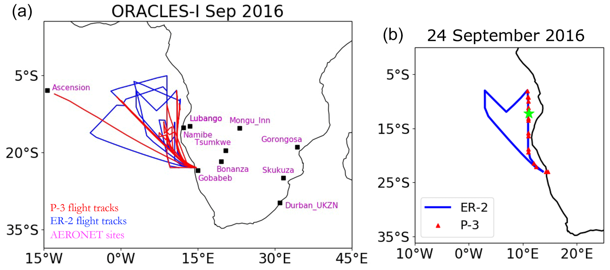
Figure 1 (a) Location of ORACLES-I P-3 and ER-2 flights off southwestern Africa during September 2016 and ground-based AERONET sites over the continent. (b) P-3 and ER-2 flight tracks for 24 September 2016, with the green star highlighting the location of the vertical profile illustrated in later plots.

Our specific objective in this study is to use the ORACLES observations to understand and improve the simulated aerosol optical properties in the GEOS model. Significantly, ORACLES-I observations showed variability in the vertical profile of the smoke SSA on several flights, possibly related to smoke plume aging (Dobracki et al., 2023; Redemann et al., 2021). Here, we utilize the GEOS model to further investigate the issue of SSA variability and present a simplistic approach to capture the observed SSA change within aging smoke plumes for chemistry transport models. After tuning the model aerosol optics and lifetimes based on ORACLES aircraft observations, we utilize the larger spatial coverage of the satellite and ground-based observations to evaluate the model aerosol properties over the complete southern African biomass burning source and outflow regions.

The paper is organized as follows: Sect. 2 provides a brief description of the observations used in this study, along with the description of the model set-up and various capabilities of GEOS that we utilize to complement our analysis. Section 3 discusses the model–data comparisons and the radiative implications of tuning the aerosol properties. Finally, Sect. 4 summarizes the major findings of our study and discusses future directions for subsequent modeling studies in this regard.

2 Approach and methods

2.1 ORACLES 2016 aircraft-based observations

We provide here brief details of the instruments relevant to our study based on the particle properties measured. Further details of the ORACLES-I instrumentation and related uncertainties are provided in Shinozuka et al.(2020), Redemann et al. (2021), and references therein.

2.1.1 Aerosol optical properties

The Hawaii Group for Environmental Aerosol Research (HiGEAR) operated several in situ instruments on the P-3. These include two Radiance Research particle soot absorption photometers (PSAPs) to measure the aerosol absorption coefficients (at 470, 530, and 660 nm), and two TSI (model 3563) nephelometers (at 450, 550, and 700 nm) to measure the aerosol light scattering coefficients. In addition to the TSI nephelometers, two single wavelength nephelometers (at 540 nm, Radiance Research, M903) were operated concurrently to measure the increase in light scattering as a function of RH. The humidified nephelometer was operated close to 80 % RH, while the dry unit was maintained below 40 % (Howell et al., 2006; Pistone et al., 2019). For in situ SSA or extinction calculation, the measured PSAP absorption was interpolated to nephelometer wavelengths before combining with its scattering data. For both SSA and extinction, we use the corrected or processed data (called SSA_ATP and Exttotal_ATP) that are provided at a time resolution of 1 s within the “merged” files at the ORACLES ESPO Data Archive: https://espo.nasa.gov/oracles/archive/browse/oracles/id8. Here, PSAP absorption corrections were performed according to an updated algorithm (Virkkula, 2010) and nephelometer-measured scattering was corrected according to Anderson and Ogren (1998). The in situ SSA and extinctions are measured and reported at low (<40 %) RH. Additionally, we only use the measurements for which mid-visible dry extinctions are greater than 10 Mm⁻¹ (Pistone et al., 2019).

In addition to dry in situ SSA, we also use the retrievals of column-integrated SSA for ambient conditions from the Spectrometer for Sky-Scanning Sun-Tracking Atmospheric Research (4STAR) instrument, which was also on board the P-3. The 4STAR instrument is an airborne hyperspectral (350–1700 nm) sun photometer that can make direct-beam measurements (sun-tracking mode) for retrievals of partial-column aerosol optical depth (AOD) above flight level (LeBlanc et al., 2020). Under ideal flight and atmospheric conditions, 4STAR can also perform sky scans in either the principal plane or almucantar (sky-scanning mode). The 4STAR sky scans were processed using a modified version of the version 2 Aerosol Robotic Network (AERONET) retrieval algorithm described in Dubovik and King (2000). However, due to suspected stray light contamination within the 4STAR spectrometer around 440 nm (Pistone et al., 2019), the set of input wavelengths for 4STAR were modified to be 400, 500, 675, 870, and 995 nm (as opposed to the standard AERONET input wavelengths). We used the quality-screened data available at the ORACLES ESPO Data Archive and presented in Pistone et al. (2019), but we further limit our analysis to SSA retrievals that had AOD_400 nm>0.4 similar to what AERONET uses in its quality control criteria. Additionally, we only consider the SSA retrievals for which flight altitude was greater or equal to 1 km, which is about the typical boundary layer height over the ocean for the ORACLES 2016 region. Since 4STAR retrieves the above-aircraft column SSA, our last screening criterion was used to focus on the SSA of smoke layers above the boundary layer and exclude the influence of marine aerosols within the boundary layer.

We also use the atmospheric profiling provided by the NASA Langley Research Center High Spectral Resolution Lidar (HSRL-2, Hair et al. (2008)) that was deployed on the ER-2 aircraft. Note that flight paths for the P-3 and ER-2 only partly overlapped (Fig. 1a), for example on the 24 September case (Fig. 1b) that we analyze in greater detail to utilize this synergy between the two aircraft (Sect. 3.1). HSRL-2 measures aerosol backscatter and depolarization at 355, 532, and 1064 nm and aerosol extinction at 355 and 532 nm. Out of the standard aerosol data products (Burton et al., 2012) that HSRL-2 provides, we use the aerosol extinction and lidar ratio (extinction-to-backscatter ratio) profiles at 355 and 532 nm for this study, both provided in 60 s averages to improve the instrument signal-to-noise ratio (equates to ∼12 km along-track horizontal resolution of the aircraft).

2.1.2 Aerosol composition

The Single Particle Soot Photometer (SP2) was deployed on the P-3 as part of HiGEAR to measure the mass of refractory black carbon (rBC) particles by passing a powerful laser beam and heating them to incandescence (Schwarz et al., 2006). The peak value of this incandescence signal has been shown to linearly correlate with the mass of the rBC particle (Stephens et al., 2003). The bulk submicrometer non-refractory aerosol composition, on the other hand, was provided by the time-of-flight (ToF) Aerodyne aerosol mass spectrometer (AMS) in the form of organic aerosol (OA), sulfate (SO₄), nitrate (NO₃), and ammonium (NH₄) mass concentrations (DeCarlo et al., 2008). The AMS-measured mass concentrations are provided at standard temperature (273 K) and pressure (1000 hPa), but we convert them here to ambient conditions using the ideal gas law and measured pressure and temperature information before comparing with the model equivalents.

2.1.3 Aerosol size distribution

Particle size distributions used in this study were measured from the P-3 with an ultra-high-sensitivity aerosol spectrometer (UHSAS, Droplet Measurement Technologies, Boulder CO, USA) with a fuselage-mounted inlet. UHSAS is an optical-scattering, laser-based aerosol particle spectrometer that measures particles from 60–1000 nm at 1 s time resolution, thereby covering the entire accumulation mode. The UHSAS measured size distribution is reported as particle number concentrations (in cm⁻³) for size bins that are approximately logarithmically spaced.

2.1.4 Carbon monoxide (CO)

CO was measured from the P-3 with a gas-phase CO $/$ CO₂ $/$ H₂O analyzer (ABB/Los Gatos Research CO $/$ CO₂ $/$ H₂O analyzer known as COMA) with an inlet mounted on the aircraft fuselage. It uses off-axis integrated cavity output spectroscopy (ICOS) technology to make stable cavity enhanced absorption measurements of CO, CO₂, and H₂O in the infrared spectral region (Provencal et al., 2005). The measurements were reported as dry air volume mixing ratios in parts per billion (ppbv).

2.2 Ground-based observations

The Aerosol Robotic Network (AERONET) measures the spectral aerosol optical thickness (AOT) through a ground-based network of sun- and sky-scanning photometers (Holben et al., 1998). For September 2016, Fig. 1a depicts the sites that were operational over southern African biomass burning source regions during ORACLES-I. AERONET provides spectral AOT to an accuracy of ±0.015 from direct sun measurements. In our analysis we use the version 3, level 2 (cloud-screened, quality-assured), AERONET direct-sun-derived AOT product, specifically the AOT at 500 nm, as well as the spectral SSA retrievals at 440, 675, 870, and 1020 nm (Giles et al., 2019; Sinyuk et al., 2020).

2.3 Satellite observations

2.3.1 OMI absorbing aerosol index

We use space-based aerosol observations from the Ozone Monitoring Instrument (OMI; Levelt et al., 2006) on board the NASA Aura spacecraft, which flies in a polar orbit with a local Equator-crossing time of 13:30 UTC. OMI is a hyperspectral (270–500 nm), wide swath (∼2600 km) imager that observes the back-scattered solar radiation with a nominal ground pixel size of 13×24 km² at nadir and 13×150 km² at the swath edges. Aerosol products are from the OMAERUV algorithm (version 1.8.9.1, after Torres et al., 2007). Fundamental to the OMAERUV retrieval is the so-called aerosol index (AI). The AI is computed from the observed radiances at two channels where ozone absorption is weak (354 and 388 nm for OMAERUV), where the observed spectral contrast is compared to the (easily characterized) spectral contrast expected in a purely molecular atmosphere. Under cloud-free conditions the AI is sensitive to aerosol loading, height, and absorption, where increases in any of those quantities result in a higher positive magnitude value of the AI. The OMI swath ideally provides near-daily global coverage but has been impacted by a “row anomaly” defect since shortly after launch that has effectively degraded its coverage by about 50 % so that OMI now achieves global coverage every two days (Torres et al., 2018). In our comparisons that follow we sample model output only where valid OMI data are collected. Owing to its relatively large pixel size OMI data are frequently cloud contaminated. We restrict our analysis to the best available data, where the algorithm quality-assurance flag is 0.

2.3.2 MODIS NNR (neural net retrieval)

The Moderate resolution Imaging Spectroradiometer (MODIS) sensors have been flying on two spacecraft, Terra (10:30 LST, local solar time, Equator crossing) since 2000 and Aqua (13:30 LST Equator crossing) since 2002. The MODIS collection 6.1 algorithms (namely, Dark Target Land, Dark Target Ocean, and Deep Blue) retrieve aerosol properties over both ocean and land surface types using the observed spectral reflectance (Levy et al., 2013). However, instead of directly using the MODIS operational retrievals of AOD for model evaluation, we use a bias-corrected AOD dataset, called the MODIS NNR, which was derived initially for use in the Modern-Era Retrospective analysis for Research and Applications, version 2 (MERRA-2, Randles et al., 2017) aerosol reanalysis. As much care as is taken in creating the MODIS standard products, there are nevertheless significant biases related to cloud and land features that must be screened prior to using these data in assimilation systems (e.g., Zhang and Reid, 2006). The NNR refers to a neural net retrieval algorithm that computes AERONET-calibrated AOD from satellite-based radiances, in this case the same MODIS collection 6.1 radiances used in the standard retrieval products. To derive 10 km resolution MODIS NNR AOD, over-ocean predictors include MODIS level 2 multichannel TOA reflectances, glint, solar and sensor angles, cloud fraction (pixels are discarded when cloud fraction >70 %), and albedo derived using GEOS surface wind speeds. Over land, predictors are the same, except a climatological albedo is included for pixels with surface albedo <0.15. The NNR algorithm is trained on the log-transformed AERONET AOD interpolated to 550 nm and co-located with MODIS observations of the predictors. Application of the NNR to the MODIS products is found to produce a higher-quality AOD product compared to (relatively unbiased) AERONET observations (Randles et al., 2017).

2.4 Model description

Simulations are performed with a version of the NASA GEOS model (Molod et al., 2015), a global Earth system model used for near-real-time weather and aerosol prediction, performing atmospheric analyses, and producing atmospheric and composition reanalyses, among other applications. The configuration of GEOS run in this study includes an atmospheric general circulation model run with the finite-volume dynamical core (FV3, after Putman and Lin, 2007) on a cubed-sphere horizontal grid. The model physics includes the Grell–Freitas deep convection (de Freitas et al., 2018; Grell and Freitas, 2014) and Park and Bretherton (2009) shallow convection, the Lock turbulence scheme (Lock et al., 2000), the catchment land surface model (Koster et al., 2000), Rapid Radiative Transfer Model (RRTMG) shortwave and longwave radiation (Iacono et al., 2008), and parameterized chemistry (Nielsen et al., 2017). An aerosol-aware single-moment cloud microphysics scheme is employed to provide dynamic cloud and ice effective radii (Bacmeister et al., 2006).

The aerosol scheme utilizes an updated version of the Goddard Chemistry, Aerosol, Radiation, and Transport (GOCART) module (Colarco et al., 2010; Chin et al., 2002). GOCART includes the sources, sinks, and chemistry of dust, sea salt, nitrate, sulfate, and carbonaceous aerosols. Dust and sea salt have dynamic (i.e., wind-driven) sources, and for each example the aerosol particle size distribution is discretized into a series of five non-interacting size bins. Bulk sulfate mass is tracked, with primary emissions from anthropogenic sources and precursor emissions of dimethylsulfide (DMS), which has emissions calculated using an empirical formula (Liss and Merlivat, 1986) that is a function of observed DMS surface concentrations (Lana et al., 2011) and 10 m wind speed, and sulfur dioxide (SO₂), which has emissions from anthropogenic, volcanic, and biomass burning sources. Chemical production of sulfate from precursors uses a simplified OH-H₂O₂-NO₃ scheme, with oxidants provided from the MERRA-2 GMI full-chemistry simulation (Strode et al., 2019). Nitrate is represented by three non-interacting size classes and has precursor emissions from anthropogenic, biomass burning, and ocean sources of ammonia. The fine-mode nitrate includes heterogeneous formation from nitric acid on dust and sea salt surfaces (Bian et al., 2017). Carbonaceous aerosols are partitioned into three compositional species – black carbon (BC), organic carbon (OC), and “brown” carbon (BR) – where each species is further divided into hydrophobic and hydrophilic modes. In the context of our simulations, “brown” carbon is organic carbon from biomass burning sources, separated from other anthropogenic and biogenic sources of organic aerosol to treat the optical properties distinctly (Colarco et al., 2017). A simplified secondary organic aerosol (SOA) mechanism is employed that scales volatile organic carbon (VOC) emissions in terms of CO emissions from anthropogenic, biofuel, and biomass sources, following Kim et al. (2015), with conversion of VOC to SOA modeled using a simple function of the MERRA-2 GMI-provided OH fields and the SOA going to hydrophilic modes of organic and brown carbon. Biogenic sources of SOA are from an online version of the MEGAN (Model of Emissions of Gases and Aerosols from Nature) mechanism running inside GEOS. Baseline optical properties are primarily based on the OPAC (Hess et al., 1998) database (see also Chin et al., 2002), with the optical properties for non-spherical dust particles based on Colarco et al. (2014), and the optical properties of brown carbon based on Colarco et al. (2017). Optical properties are defined in pre-computed lookup tables that are a function of species, wavelength, and relative humidity (to account for particle humidification). In situ optical quantities such as extinction and SSA are computed by summing across the aerosol species concentrations as scaled by the appropriate optical property (e.g., mass extinction efficiency). Column-integrated optical quantities (e.g., AOD and SSA) are computed as the vertical integral of the in situ properties. The aerosol species are externally mixed in the model for optics and chemistry purposes.

Biomass burning emissions in our simulations are based on the Quick Fire Emission Dataset (QFED; Darmenov and da Silva, 2015). QFED utilizes satellite fire radiative power observations from MODIS Level 2 fire products and scales them using biome-specific emission factors to aerosol and trace gas emission fluxes. In this study we particularly use QFED emission products for SO₂, CO, NH₃, BC, and OA. Here (and throughout the rest of the paper), model OA refers to organic aerosol contributions from all sources (biomass, biogenic, biofuel, and anthropogenic) unless specifically mentioned.

Our baseline GEOS simulation is performed at a c360 (∼25 km) horizontal resolution with 72 vertical hybrid sigma levels extending from the surface to ∼80 km altitude. The model is “replayed” to the European Centre for Medium-Range Weather Forecasts (ECMWF) fifth-generation atmospheric reanalysis (ERA5, Hersbach et al., 2020). “Replay” mode is like running the model in an atmospheric data assimilation mode, but instead of ingesting the meteorological observations directly we use the atmospheric state (surface pressure and vertical temperature, humidity, and horizontal wind components) from a prior analysis and compute the model incremental analysis update (IAU) from the forecast model background state versus that analysis, in this case versus ERA5. This approach allows us to perform a simulation constrained by realistic meteorology at a fraction of the cost of performing the full atmospheric data assimilation cycle. ERA5 was chosen to replay against versus the GEOS-native MERRA-2 (Gelaro et al., 2017) because sensitivity simulations (not presented here) showed a more favorable representation of the smoke plume vertical distribution transported from southern Africa (see also Das et al. , 2017, for a discussion of the challenges of models in representing the vertical profile of smoke in this region). Table 1 summarizes the suite of GEOS simulations performed in this study that are described in subsequent sections of the text.

Table 1 Summary of GEOS simulations performed in this study.

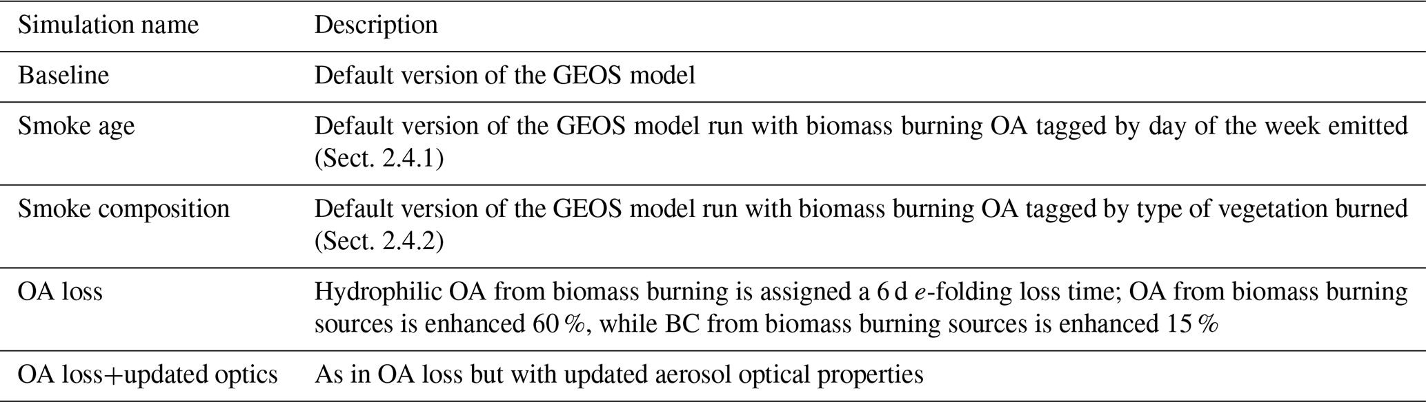
2.4.1 Estimation of physical smoke age

Our “smoke age” simulation (see Table 1) has the brown carbon tracer “tagged” in such a way as to determine the day of the week on which its emissions were injected. Effectively, eight instances of the biomass burning organic aerosol are tracked in this simulation (seven instances, one for emissions occurring each day of the week, and an eighth for the cumulative total emissions). The “Monday” tracer, for example, resets the tracer concentration globally to zero when the model clock ticks over to Monday at 00:00 UTC. The differences between the total and individual day-of-the-week tracers allows determination of the smoke age out to smoke emitted 7 d previously. The simulation is otherwise identical to our baseline simulation.

2.4.2 Estimating the smoke composition based on their emission source vegetation type

Our “smoke composition” simulation has the biomass burning OA tagged by the vegetation source burned based on the QFED inputs. QFED biomass burning emission sources are classified using the land cover or vegetation type information provided by the MODIS Land Cover Type Product (MCD12C1, IGBP classification scheme, Friedl et al. , 2010) for the year 2016, shown in Fig. 2. The MCD12C1 product supplies global maps of land cover at annual time steps at 0.05° spatial resolution in geographic latitude–longitude projection. Further details on the Collection 6 MODIS Land Cover products, including MCD12C1, are provided in their User Guide: https://lpdaac.usgs.gov/documents/101/MCD12_User_ Guide_ V6.pdf, last access: 5 December 2023. We define six major vegetation or land cover (LC) types over central and southern Africa that could contribute to the smoke over ORACLES region: (1) savannas (LC type 9), (2) woody savannas (LC type 8), (3) grassland (LC type 10), (4) tropical forest (LC type 2, 4, 5), (5) shrubland (LC type 6,7), and (6) croplands (LC type 12, 14) (Fig. 2). We then define seven instances of brown carbon tracers (six are “tagged” based on their emission source vegetation type, plus one for the total) within the model to be able to investigate the contributions of each of these vegetation types towards the smoke observed over the ORACLES region.

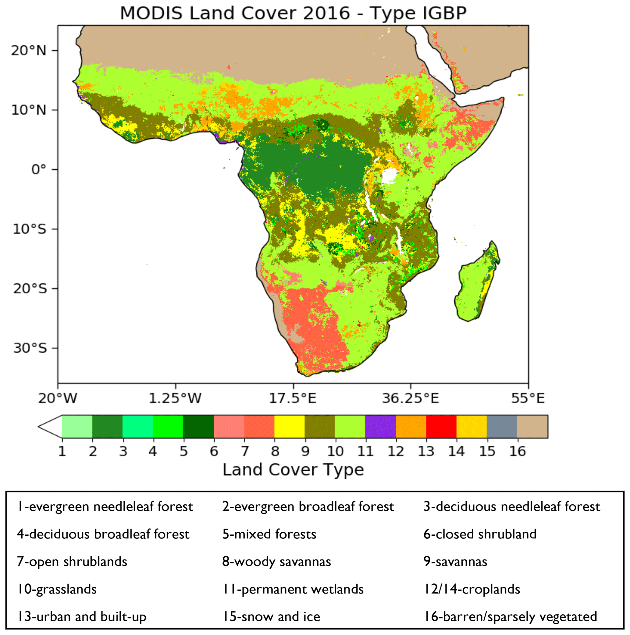
Figure 2 Land cover or vegetation types for 2016 from the MODIS Land Cover Type Product (MCD12C1) using the IGBP classification scheme.

2.4.3 OMI AI simulator

We employ a radiative transfer code to simulate the OMI aerosol index (Buchard et al., 2015; Colarco et al., 2017). Similar to the computation of the model AOD, the AI simulator takes the GEOS-simulated aerosol mass distributions and meteorological fields as input, and – subject to the GEOS aerosol optical property assumptions – simulated OMI radiances are calculated at the OMI viewing conditions (viewing geometry, terrain height, and surface reflectance). AI is then calculated as in Colarco et al. (2017). Because we do not explicitly simulate the impact of modeled cloud fields on the simulated radiance, we restrict our comparisons to the highest-quality OMI retrievals (formally, QA flag = 0) to eliminate cloudy pixels in the satellite product impacting our comparisons as much as possible.

2.5 NOAA HYSPLIT model with ERA-5 meteorological fields

We use the Linux-based distribution of the NOAA (National Oceanic and Atmospheric Administration) Hybrid Single-Particle Lagrangian Integrated Trajectory (HYSPLIT, v5.2.1) model (Rolph et al., 2017; Stein et al., 2015) to understand the transport pathway and origin source locations of the smoke observed during ORACLES 2016. ERA-5 meteorological data are used to drive HYSPLIT so that the trajectories calculated are consistent with our GEOS simulations. We employ the meteorological grid ensemble approach within HYSPLIT to quantify the uncertainty and divergence associated with the trajectory calculations. In this method, trajectories are computed for a three-dimensional cube centered on the starting point. Instead of moving the trajectory initial location about the starting point, all the trajectories start from the initial point, but the driving meteorological data for each trajectory are offset slightly from that central location (see https://www.ready.noaa.gov/documents/Tutorial/html/traj_ensem.html, last access: 7 December, 2023). Default offsets are chosen so that the meteorology is spread one grid box in the horizontal (∼25 km) and about 250 m in the vertical. This results in 27 members of the trajectory ensemble for all possible offsets in X, Y, and Z directions in space.

3 Results and discussion

In the following we analyze the ORACLES airborne data and our GEOS simulations, first for the specific case of the aerosol plume flown by the P-3 and ER-2 on 24 September 2016. Refinements to our simulations are then described. We conclude by summarizing our simulation of the entire month of September 2016 in the context of ground-based and space-based remote sensing observations and estimate the total aerosol radiative forcing during the month.

3.1 The 24 September 2016 case

We focus here on the 24 September 2016 smoke plume observed from both the P-3 and ER-2 aircraft (Fig. 1b). We choose this day for two main reasons: (1) the presence of multi-layered smoke around 12° S, 11° E that showed a gradual but substantial change in the in situ measured SSA vertically (from 0.83–0.91 over 1–5.5 km respectively) that GEOS was unable to capture in our baseline simulation and (2) to utilize the synergy of multiple instruments on board both the P-3 and ER-2 aircraft as they sampled the same locations for a significant part of their flight.

On 24 September, the P-3 flew an out-and-back, south-to-north-to-south flight along 11° E longitude to and from Walvis Bay, Namibia (Fig. 1b). The P-3 vertical flight profile is shown in Fig. 3 with the in situ (PSAP and nephelometer) measured dry extinction superimposed on the baseline GEOS-simulated extinction profile sampled in space and time along the flight track. The out-and-back nature of the flight track is evident in the model fields, which show a quasi-symmetric vertical profile in time. The blue stars in Fig. 3 indicate the location of 4STAR sky scans for which quality-screened, column-integrated SSA were retrieved (Pistone et al., 2019). On the same day the ER-2 aircraft carrying the HSRL-2 lidar spatially overlapped with part of the P-3 flight path (Fig. 1b). The retrieved and GEOS-simulated vertical aerosol extinction profile (GEOS sampled along the ER-2 track) are shown in Fig. 4. A similar aerosol plume structure is apparent in GEOS comparisons of these two sets of observations (Figs. 3 and 4).

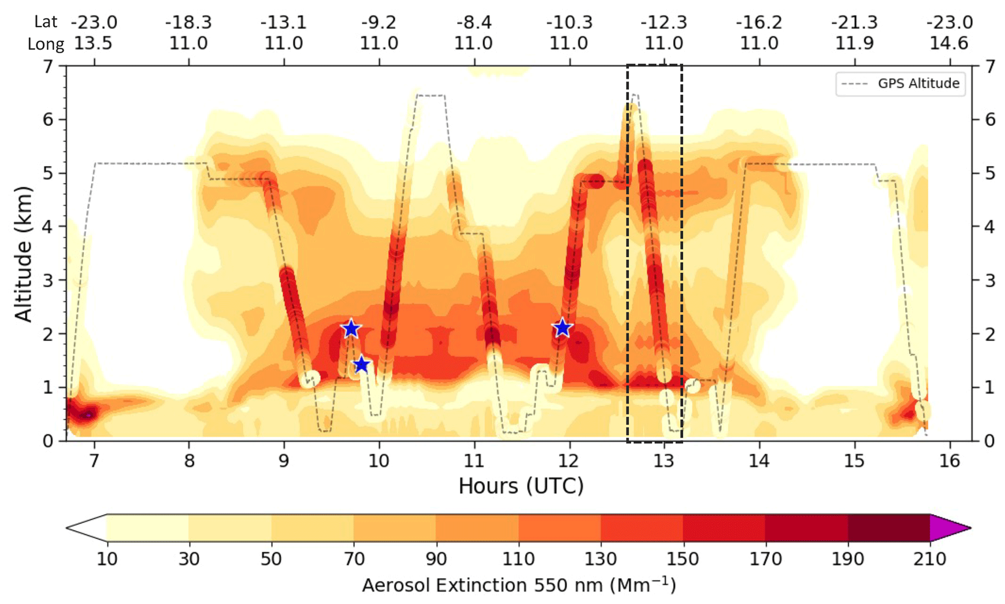
Figure 3 Background is the 550 nm extinction profile simulated in the GEOS baseline run along the P-3 flight track on 24 September 2016. Overplotted are the P-3 measured extinction values. The dashed gray line shows the P-3 flown altitude profile along the track. The dashed black box centered at 13:00 UTC shows the location of the specific profile highlighted by the green star in Fig. 1b and analyzed in later plots. Blue stars are the locations of specific 4STAR SSA retrievals analyzed later.

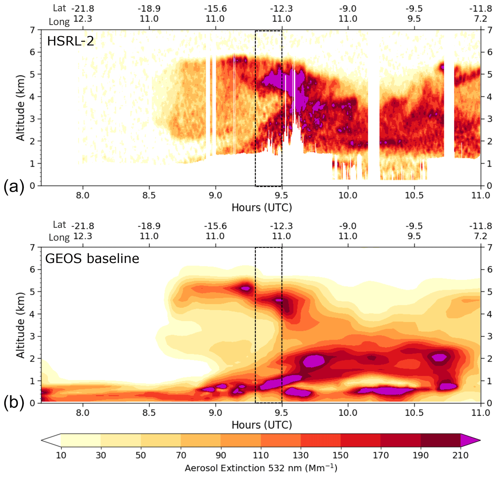
Figure 4 (a) HSRL-2 observed 532 nm extinction profile along the ER-2 flight track on 24 September 2016. (b) GEOS baseline simulated 532 nm extinction profile along the same flight track. Dashed boxes near 9.5 UTC indicate the position of the profile compared to the P-3 profile in subsequent plots and referenced by the green star in Fig. 1b.

Between 12:45 and 13:01 UTC the P-3 sampled a multi-layered smoke plume around 12.3° S, 11° E while descending from 6 to 1 km. The ER-2 flew over the same location earlier in the day, and this common spatial region is shown by the rectangular black box in Figs. 3 and 4 and is indicated by the green star in Fig. 1b. For purposes of comparison, we averaged the ER-2 HSRL profiles over the same area covered during the P-3 profile (from 09:15 to 09:30 UTC, black box in Fig. 4). We compared the observed aerosol extinctions for this profile based on in situ instruments (Fig. 5a) and HSRL-2 lidar (Fig. 5b) with our GEOS baseline simulation. The in situ observations are made under dry conditions (RH < = 40 %), while the lidar observations are at ambient conditions. An elevated smoke layer was observed from both aircraft between 4–6 km altitude and a lower layer between about 1.5–3.5 km altitude. Figure 5c shows the P-3 measured temperature for this profile, as well as the dry and moist adiabats anchored at 2 km. The slope of the observed temperature profile is greater than the dry adiabatic lapse rate but less than the moist adiabatic lapse rate, indicating conditionally stable air layers that explain the distinct plumes over the ocean, also a feature over land (Tyson et al., 1996). Additionally, the high relative humidity at the upper layer (RH ∼ 80 %, Fig. 5c) suggests humidification could be part of the explanation for the higher aerosol extinction (peak extinction ∼100 Mm⁻¹ at 4.5 km altitude) compared to the in situ measurement (∼150 Mm⁻¹ at the same altitude). The GEOS simulated dry extinction is underestimated compared to the in situ data (peak of ∼100 Mm⁻¹) but has a better match with HSRL-2 retrieval at ambient conditions (∼175 Mm⁻¹), at least for the upper-level smoke layer. The model profile of humidity agrees well with the observations (Fig. 5c), so the difference in extinction suggests that the model has more hygroscopic growth of the smoke for the higher-altitude plume than the observations suggest, a point we will return to later. The model-simulated ambient extinction is underestimated for the lower aerosol layer despite a good match of simulated RH with the observations overall (Fig. 5c).

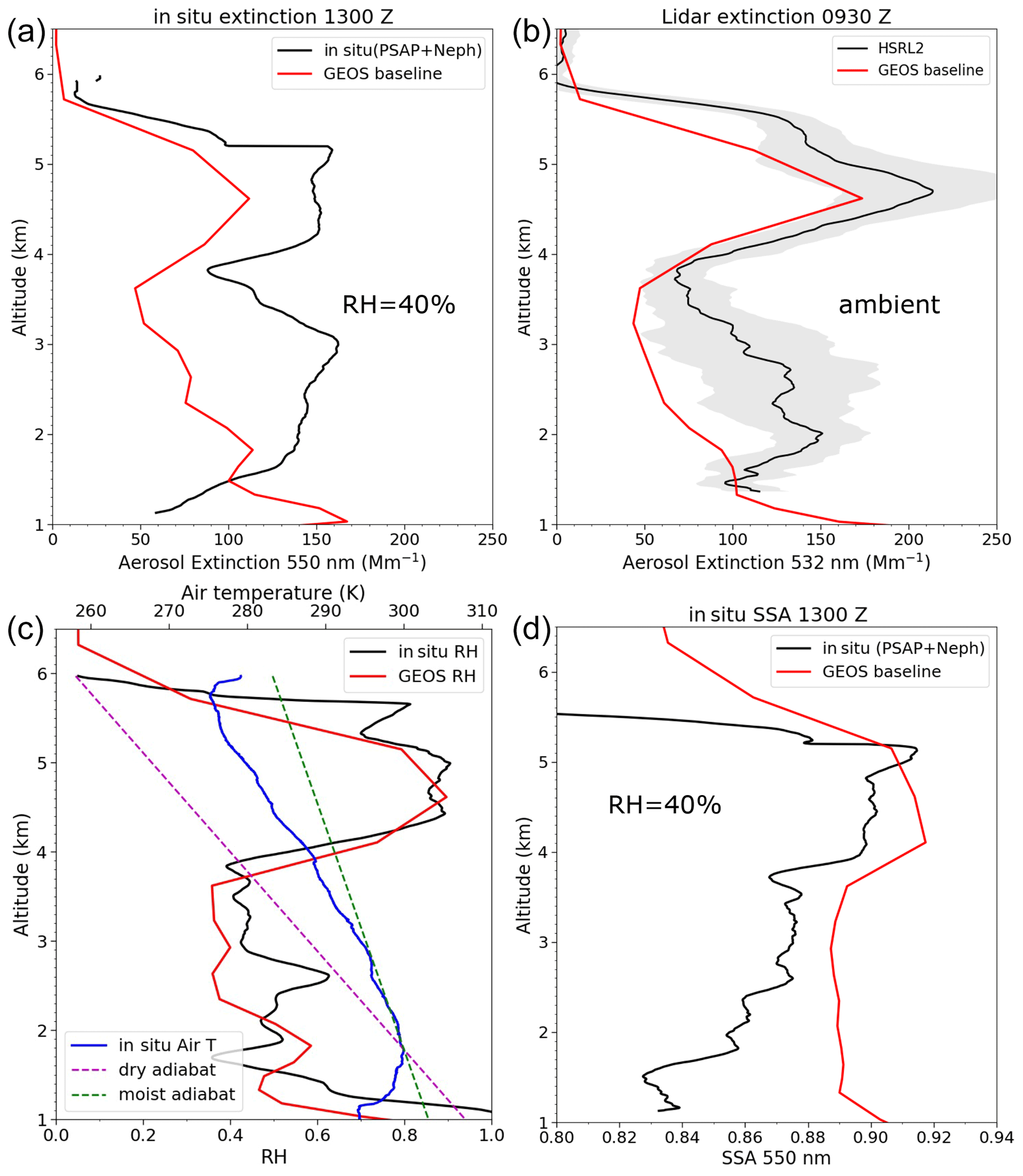
Figure 5 Profiles of the P-3 in situ measured 550 nm extinction (a) for the point indicated by the green star in Fig. 1b and ER-2 HSRL-2 lidar 532 nm mean extinction (b) for the same location enclosed within the rectangular box in Fig. 4b. The gray shading in (b) represents the ±1 standard deviation around the lidar-observed mean extinction. Also shown are the P-3 measured relative humidity and ambient air temperature (c), along with the 550 nm single-scatter albedo (d). In each plot the data are indicated by the black line, and the GEOS baseline simulations in the profiles are indicated by the red line.

We compare the observed and simulated SSA on this profile in Fig. 5d. The in situ measurements of dry SSA at 550 nm showed a gradual decrease in values from about 0.92 to 0.84 between the altitudes of 5.5 to 1 km, respectively. The model simulations of SSA, on the other hand, showed some decrease from the aerosol layer centered around 4.5 km to the lower altitude layers but stayed fixed at about 0.89 from 4 to 1 km altitude. Clearly the baseline GEOS model does not simulate the observed vertical variability in SSA.

3.1.1 Composition, SSA, and relation with simulated smoke age

To understand the vertical variations in SSA, we first analyze the smoke composition of this 24 September profile by comparing the model-simulated aerosol mass concentrations to the corresponding measurements from the AMS and SP2 in situ instruments (Fig. 6). Organic aerosols (from all sources) contribute about 65 %–70 % of the total aerosol mass, followed by nitrates, sulfate, and BC in both the model and the observations. Model-simulated aerosol composition agrees well with in situ observations, especially for the top plume centered around 4.5 km (where both show peak OA mass concentration ∼17 µg m⁻³). OA is overestimated by the model for altitudes below 2.5 km (Fig. 6a), while nitrates are underestimated for the same altitudes (Fig. 6c). Sulfate (Fig. 6d) and BC (Fig. 6b) show a similar profile shape to the simulated OA but are present at lower concentrations than the observations suggest, particularly for the lower-altitude layer. Sulfate is about half the concentration in the model as observed. BC has similar concentration to the observations for the higher smoke plume (∼1 µg m⁻³) but is only about half the concentration of the observations in the lower layer. Except for nitrate, the observed multi-layer structure for this profile is evident in the model species.

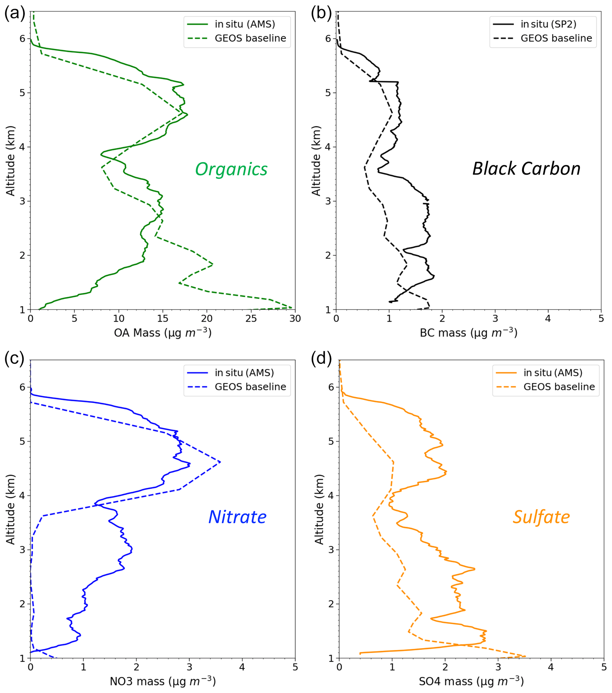
Figure 6 Comparison of the in situ measured (solid lines) and GEOS baseline model-simulated (dashed lines) aerosol species mass concentrations on the P-3 profile flown near 12° S, 11° E on 24 September 2016. Shown are (a) organic aerosol, (b) black carbon, (c) nitrate, and (d) sulfate mass concentrations.

SSA strongly depends on the relative amounts of scattering to absorbing aerosols. BC is the primary absorbing component at 550 nm in the smoke plumes simulated here, while OA, nitrates, and sulfates are mostly scattering. Given that the SSA is changing with altitude (Fig. 5d) and multiple plumes are observed within the vertical profile (Fig. 5a), we investigate the following two things: (1) the smoke age in the vertical and (2) how the relative aerosol composition varies with altitude and smoke age. Figure 7a shows the model-simulated, extinction-weighted mean smoke age for our 24 September profile using our smoke age tagged tracer run (described in Table 1 and Sect. 2.4.1). Fig. 7a also shows the smoke age derived using the WRF-AAM (Weather Research and Aerosol Aware Microphysics) model (Saide et al., 2016) that was used for forecasting and flight planning during the ORACLES campaign (Redemann et al., 2021). The GEOS and WRF-AAM models have a similar overall structure of simulated plume age, showing minimal smoke age around the center altitude of the upper smoke plume (∼4 d at 4.5–5 km altitude) and higher smoke age at lower altitudes, with a local maximum of about 5–6 d between 3–4 km and increasing to 7–8 d below 2 km. We also show the smoke age distribution from our GEOS smoke age run at three different altitudes of the profile to clarify the interpretation of the mean smoke age number and to note some of the limitations of model-calculated smoke age (Fig. 7b). For example, for the youngest smoke plume centered at 4.5 km, even though the mean smoke age is calculated as 4.1 d, about 40 % of the smoke is 1–2 d old, while about 20 % of the smoke is older than 7 d, suggesting quite a wide distribution. At 3 km altitude the lower mode of the smoke age distribution peaks at 2–3 d old, and at 2 km it peaks at 3–5 d old. We should also be mindful that different age distributions could lead to the same mean age value. Finally, for GEOS, we are restricted by the way we track the smoke age that we can only resolve smoke age up to 7 d, and older smoke is lumped into this last bin of our histogram so that the effective age computed is slightly younger than if we could account for all possible smoke ages. Nevertheless, the simulation shows the presence of generally younger smoke at higher altitudes and older smoke at lower altitudes.

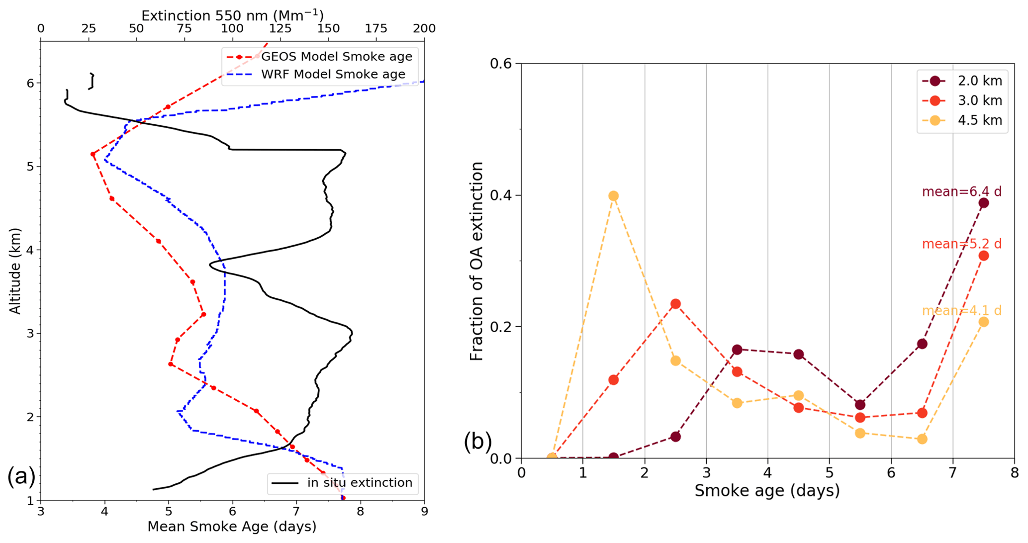
Figure 7 (a) Comparison of the GEOS baseline simulated mean smoke age (red) to WRF-AAM simulated (blue) for the smoke profile near 12°S, 11° E flown by the P-3 on 24 September 2016. The in situ extinction profile (black) is overlaid in (a) to demonstrate the differences in simulated smoke age between the multiple observed smoke layers. (b) Distribution of simulated smoke ages from the GEOS baseline simulation for the same plume profile at three different altitudes.

Next, we investigate how the relative composition of aerosols changes with smoke age and if we can further use that relation to explain the vertical variations of SSA as well. Figure 8a shows the simulated and observed change in SSA with the GEOS-simulated mean smoke age for the profile shown in Fig. 5d, and this variation is almost identical to the SSA variation in the vertical since smoke age and altitude show a strong negative correlation. The initial drop in SSA between 4–5.5 d estimated smoke age is correlated with a simultaneous decrease in OA and nitrates with respect to BC (Fig. 8b, c). After 5.5 d age the nitrates are essentially constant in time, and thus a further decrease in SSA with smoke age is more clearly correlated with a continued decrease in OA : BC ratio (Fig. 8b). The model captures the variation in NO₃ : BC and SO₄ : BC ratio well for most parts of the profile (Fig. 8c, d). The major discrepancy between the model and observations lies in the inability of the model to simulate the observed OA : BC variation, which changes in the observations from about 15 (for 4 d old smoke) to about 5 (for 7 d old smoke), whereas the model is essentially constant at a OA : BC ratio of 15. Figure 8e and f show, respectively, the correlation of OA : BC with SSA (r=0.89) and NO₃ : BC with SSA (r=0.88).

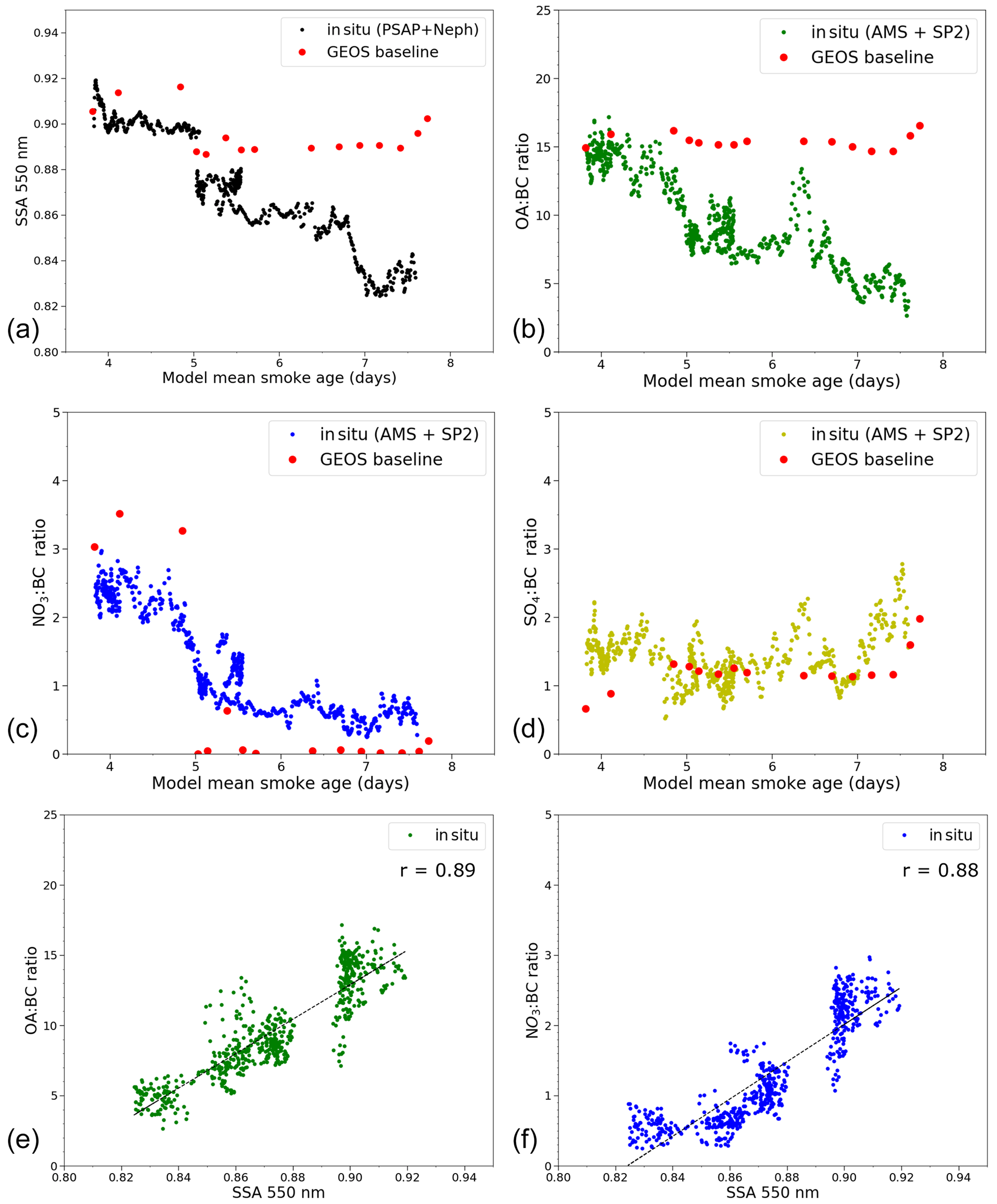
Figure 8 Observed and simulated (a) SSA at 550 nm, (b) OA : BC ratio, (c) NO₃ : BC ratio, and (d) SO₄ : BC ratio for the smoke layers near 12° S, 11° E flown by the P-3 on 24 September 2016. All of the results are sorted by mean smoke age from the GEOS baseline simulation. Also shown are the correlation of the OA : BC ratio (e) and the NO₃ : BC (f) ratio against SSA.

The model's failure to simulate the observed OA : BC ratio variability with age is correlated with its failure to simulate the observed variability in SSA. In the following we consider two hypotheses to explain the age-related variation in the OA : BC ratio. In the first we consider the possibility that smoke of different ages may be originating from different source regions with different emissions of OA and BC. In the second we consider the possibility that there is some non-simulated mechanism for the loss of OA during transport that is related to its age.

3.1.2 Are smoke layers originating from different emissions sources or burning conditions?

The first hypothesis we examine is whether smoke of different ages is originating from different source regions with different characteristics in the composition of emitted species or different proportions of the flaming and smoldering phases of the combustion products. We use three approaches to examine this hypothesis: (1) we generate ensembles of back-trajectories to track the origin of smoke layers at different vertical levels, (2) we utilize the vegetation type smoke composition tracer run of our GEOS model (Table 1, Sect. 2.4.2) to quantify the contribution of each vegetation type towards OA amounts (or extinction), and (3) we examine the observed black-carbon-to-carbon-monoxide ratios as an indicator of whether the smoke arises from flaming versus smoldering combustion. Our analysis is for the same 24 September aerosol profile discussed previously.

GEOS uses biomass burning emissions from the QFED inventory based on the MODIS fire radiative power products (Sect. 2.4). QFED provides daily gridded biomass burning emission fluxes of relevant species, such as OA, BC, and SO₂. Figure 9a shows the QFED emission locations and cumulative amounts of OA emitted over the 7 d prior to 24 September. Figure 9b and c show the HYSPLIT-model-generated ensemble back trajectories (multi-colored lines) initialized from two different vertical levels (4.5 km versus 2 km) that represent the location of the two distinct smoke plumes evident in the profile plots (e.g., Fig. 6a). For the higher-altitude smoke layer (centered around 4.5 km), the clustering of the trajectories and their intersections with the surface (where they would entrain smoke) occurs only a few days before intercepting our profile location (the black star in Fig. 9b, at 12° S, 11° E), consistent with the smoke being young (about 4 d old, Fig. 7). By contrast, the lower-altitude initialized back trajectories (originating at 2 km, Fig. 9c) intercept the surface several days back and further to the east of the profile location, consistent with the smoke at these levels being older (about 6–7 d old, Fig. 7).

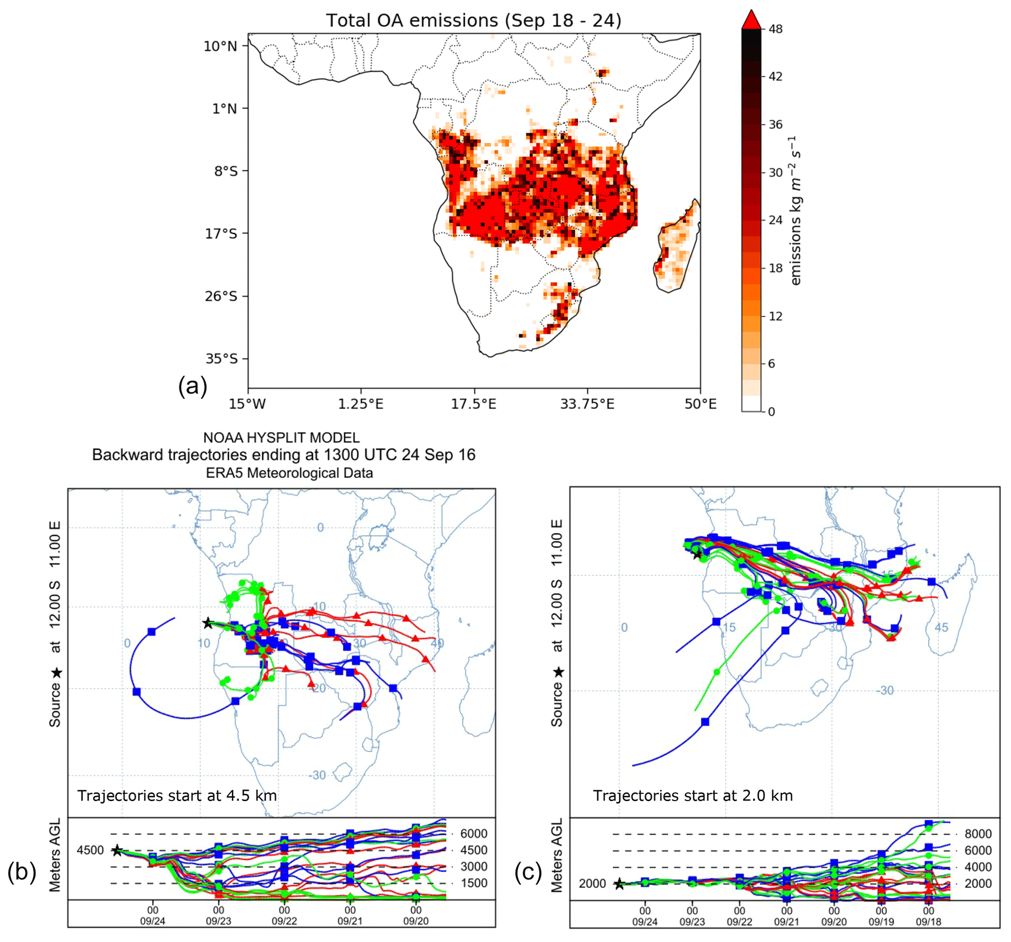
Figure 9 (a) Cumulative smoke emissions of OA over southern Africa in the week before the 24 September 2016 profile. Also shown are the ensemble of back trajectories calculated with the HYSPLIT model from the profile location initiated at 13:00 UTC on 24 September 2016, with trajectories ending at (b) 4.5 km and (c) 2 km altitude.

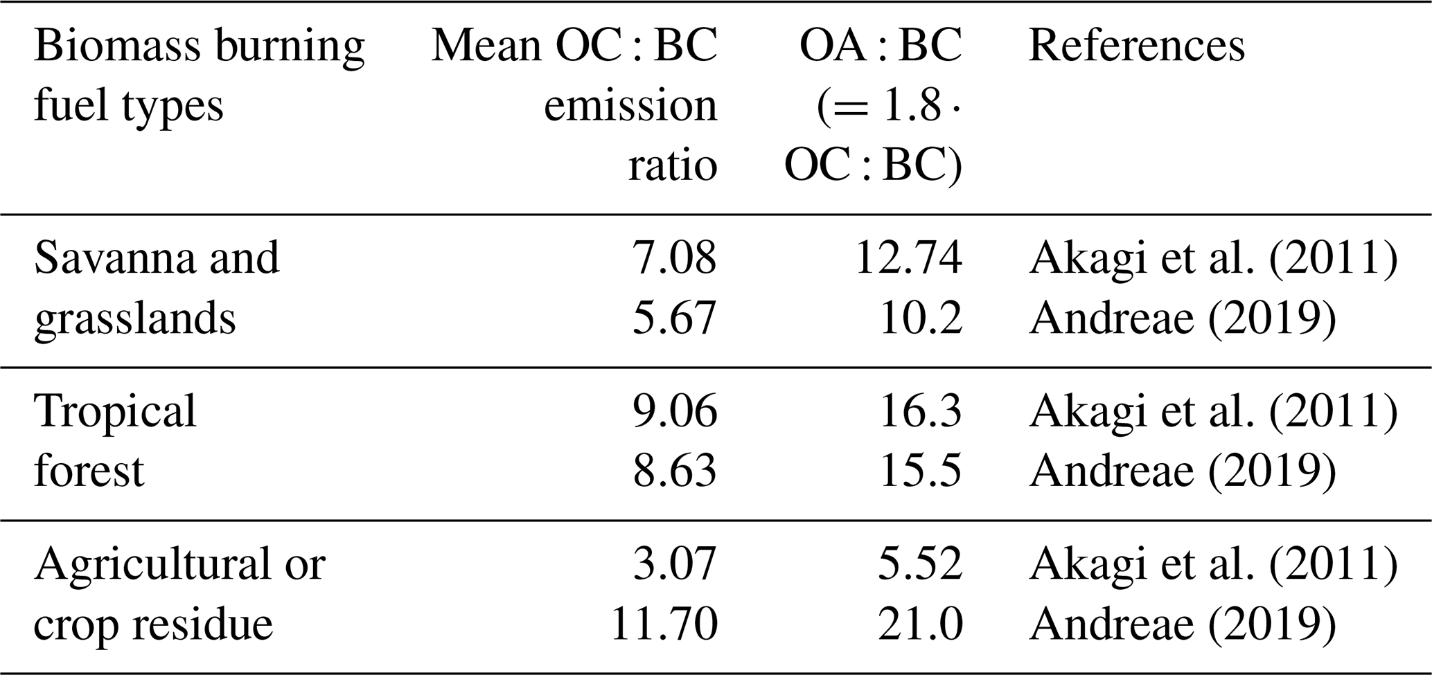
The trajectory information alone does not tell us that the composition of the smoke in the two different layers is similar. Our smoke composition simulation (see Table 1 in Sect. 2.4) is used to distinguish the contributions of individual vegetation types to the total smoke composition. QFED distinguishes among several different vegetation types according to land use datasets, and vegetation-dependent emission factors are used to scale from biomass burned to emissions of specific species (i.e., OA and BC). In the smoke composition simulation we “tag” the smoke emissions from each vegetation type so we can track its evolution separately. In Fig. 10a we quantify the contributions of emissions from individual vegetation types to the smoke composition at our profile location separately for altitudes of 4.5 and 2 km, which are the central altitudes of the two smoke plumes in the profile. Our results indicate that the major emission sources for both smoke layers are savannas, woody savannas, and grasslands. The contributions from other vegetation types (tropical forests, shrublands, and croplands) amount to only about 20 % of the total emissions. More importantly, the contributions from all vegetation types, except grasslands and woody savannas, are comparable for both the higher- and lower-level smoke plumes. The higher grassland contributions (relative to woody savannas) for the 2 km level are possibly due to smoke originating from the grassland-dominated regions south of 15° S and east of 20° E based on the 2 km back trajectories (Fig. 9c) and the land cover map (Fig. 2). However, Akagi et al. (2011) and Andreae (2019), which are the key databases that most global models use for their assumptions of emission factors of different biomass burning species, do not differentiate between grasslands and savannas as fuel types, assigning them both the same emission factors. After savannas and grasslands, the next most prevalent vegetation type contributing emissions is forest, which has a higher OA : BC emission ratio than grasslands and savannas but contributes only about 10 % to the total smoke load and is similar in contribution for both plumes. Crop and agricultural residue have distinct OA : BC ratios (that are highly uncertain; see Table 2) but are an even smaller contribution to the total aerosol load and are also a similar contribution to each layer.

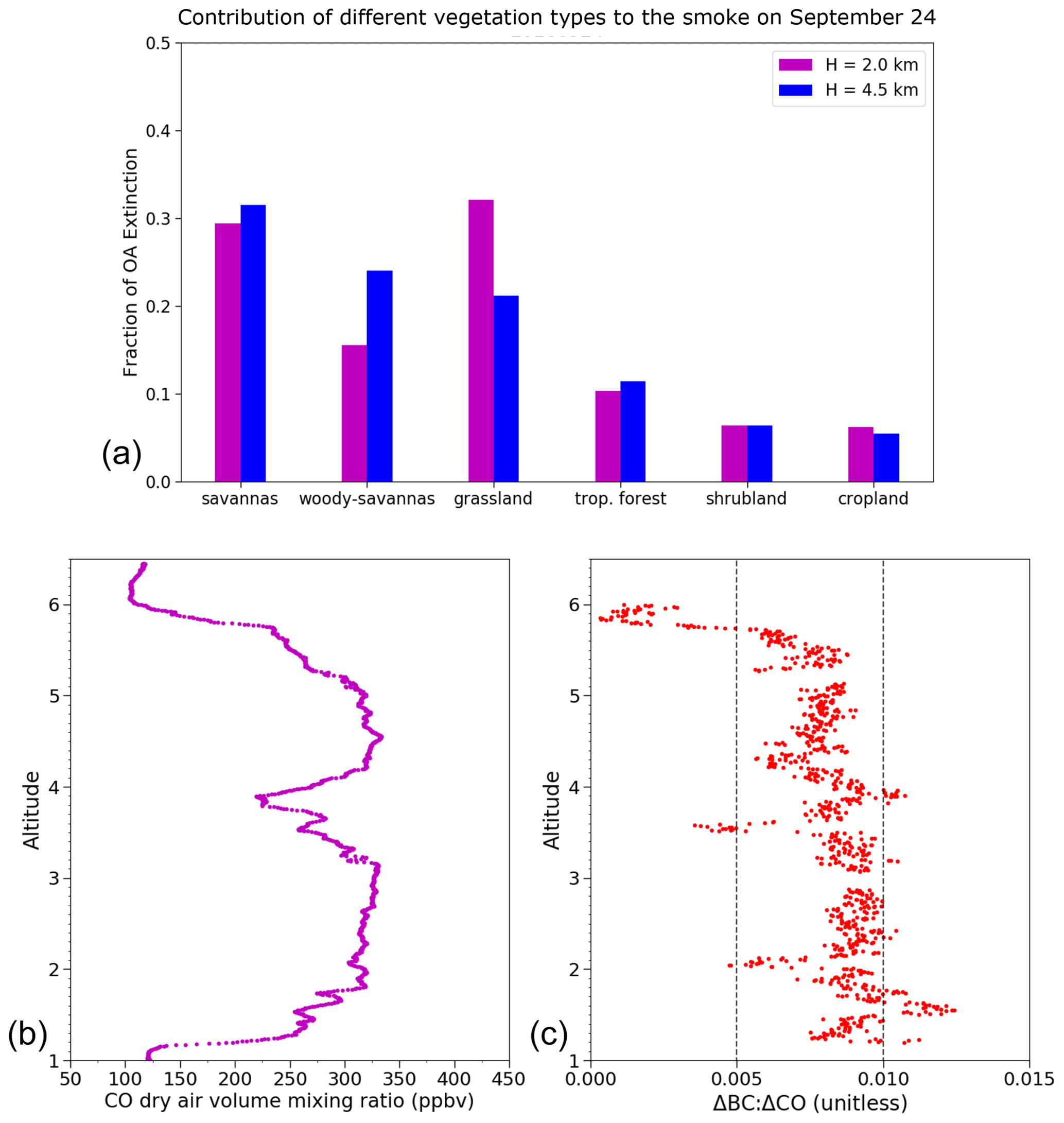
Figure 10 (a) Fraction of the OA extinction for the 24 September 2016 profile at 4.5 and 2 km altitude attributable to emissions from various types of vegetation burned. (b) P-3 observed carbon monoxide concentrations for the 24 September 2016 profile made near 12° S, 11° E. (c) Ratio of excess BC to carbon monoxide for the profile. Dashed lines demarcate regimes where smoldering (ratio < 0.005) and flaming (ratio > 0.01) conditions dominate.

Table 2 Emission ratios for different fuel types relevant to southern African biomass burning region based on two primary databases that most global models use. Akagi et al. (2011) and Andreae (2019) report emission factors for OC and BC, from which we compute the OC : BC ratio. Also shown is the OA : BC ratio used in the GEOS simulations. GEOS assumes OA : OC ratio of 1.8, based on airborne mass spectrometry measurements (Hodzic et al., 2020).

Finally, differences in the OA : BC ratio could also be due to different combustion characteristics of the source fires (i.e., flaming versus smoldering), wherein flaming fires are known to generate a lower concentration of organic carbon particles but a higher concentration of BC than smoldering fires (Christian et al., 2003; Yokelson et al., 2009). We note here that we currently do not make the distinction in emission ratios based on fire characteristics within QFED or GEOS. Vakkari et al. (2018) suggests that the excess-BC-to-excess-carbon-monoxide ratio (ΔBC $/$ ΔCO or BC : CO here onwards) can be used as a reliable marker to assess the combustion characteristics, especially for diluted and aged plumes. An increasing ΔBC $/$ ΔCO value is indicative of increasing flaming fraction during the burning (Yokelson et al., 2009). Precisely, Vakkari et al. (2018) distributed the BC : CO ratios into bins of 0.005 to represent fires of similar characteristics. Further, based on their measurements over southern African savanna and grassland regions, they found that BC : CO <0.005 represents predominantly smoldering conditions, while BC : CO >0.010 represents predominantly flaming conditions. We consider background CO to be 100 ppbv based on the values outside the plume (found at altitudes >6 km, see Fig. 10b) for the 24 September case. Figure 10c shows that the excess BC : CO ratio has very little variation in the vertical, and the values are within the range of 0.005–0.010, thereby suggesting an approximately equal mix of smoldering and flaming combustion conditions at altitudes between 1 and 5.5 km.

Based on the analyses shown here we conclude it is unlikely that the observed differences in smoke composition (i.e., the OA : BC ratio, as in Fig. 8b) at different vertical levels are due to differences in either the burning source vegetation type or combustion conditions.

3.1.3 Implementation of additional OA loss rate

The second hypothesis we consider is that there is a chemical or microphysical loss of OA during transport that is related in some way to the smoke age. OA from biomass burning sources is composed of primary organic aerosol (POA) directly emitted from the burning biomass and SOA formed via oxidative processing of organic gases. As the biomass burning plume ages in the atmosphere, the oxygenation of OA (reflected in O $/$ C ratio) is reported to increase significantly in almost all studies, suggesting strong chemical transformation of OA with aging and formation of more oxidized OA that is compositionally different from POA (Capes et al., 2008; Jolleys et al., 2012; Cubison et al., 2011; Forrister et al., 2015; Zhou et al., 2017). OA mass is increased by SOA formation but can also be balanced out by dilution and subsequent evaporation to the gas phase of semivolatile components, resulting in loss of POA mass (Cubison et al., 2011; May et al., 2015; Zhou et al., 2017). In addition, the volatilities of organic species are affected by atmospheric oxidation reactions. In the gas phase, two main processes can affect the volatilities of organics during atmospheric oxidation: fragmentation and functionalization. Fragmentation refers to the loss of carbon from the organic particles, whereas functionalization refers to an increase in particulate oxygen due to the addition of polar functional groups. Therefore, fragmentation leads to an increase in vapor pressure (i.e., the organic compounds become more volatile), while functionalization leads to lowering of vapor pressure of the organic compounds. In the condensed phase, additional bimolecular processes, such as accretion and oligomerization reactions can also affect volatility (Kroll et al., 2009). Changes in OA composition with aging inevitably lead to changes in OA optical and hygroscopic properties and thus have climate implications. The reasons for the variability across studies may be related to variations in fuels burned and combustion conditions; variation in key co-emitted species such as NO_x; and differences in environmental conditions such as dilution rate, temperature, and humidity (Shrivastava et al., 2017).

Within GEOS, the OA : BC ratio is prescribed at the point of emission based on the fuel type and related emission factors (see discussion in Sect. 3.1.2). Further, OA is emitted as 50 % hydrophobic and hydrophilic, while BC is emitted as 80 % hydrophobic and 20 % hydrophilic. Once emitted, both OA and BC undergo hydrophobic-to-hydrophilic conversion with a conversion rate or e-folding time of 1–2 d (Colarco et al., 2010). This hydrophobic-to-hydrophilic conversion can change the OA : BC ratio somewhat from what it is at emission due to wet scavenging, but for older smoke (>2 d old) we do not account for any additional OA or SOA loss due to any microphysical or chemical processes. Indeed, our simulated OA : BC ratio remains mostly constant over time, as in Fig. 8b.

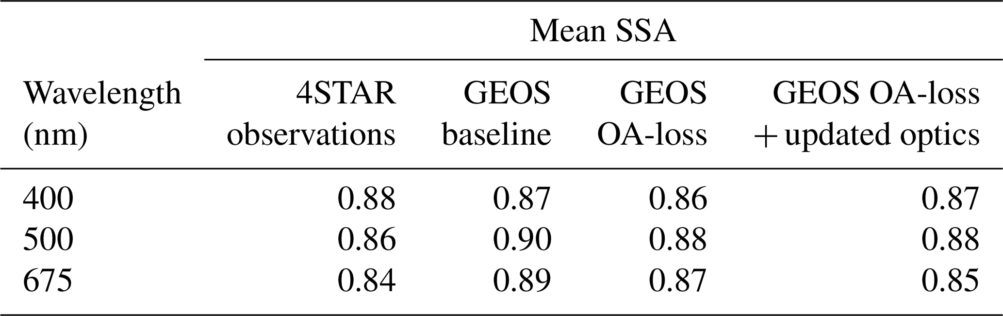
With the present model limitations in mind, we introduce an ad hoc loss process for the hydrophilic OA in our model. We additionally increase our overall emissions of biomass burning produced OA to compensate for this added loss channel to approximately preserve the overall regional extinction and AOD. Sensitivity studies suggest a 6 d e-folding time applied to the biomass burning hydrophilic OA, with a corresponding increase of about 60 % in emissions of OA and about 15 % in the BC emissions from biomass burning, greatly improves our simulated OA profile (Fig. 11a). When these factors are applied to our simulations (“OA-loss” simulation, Table 1), we can simulate the observed SSA variation with altitude well (Fig. 11b). Simultaneously, these changes resulted in overall more absorbing aerosol mixtures. Overall, there is better agreement in the SSA between 4STAR and the OA-loss simulation than 4STAR and the baseline, except at the shortest wavelength (Fig. 11c, where at 400 nm we have SSA_4STAR=0.88, SSA_Baseline=0.87, and SSA_OA-loss=0.86, and at longer wavelengths the SSA_OA-loss is closer to 4STAR than the baseline by a magnitude of 0.02; see also Table 3).

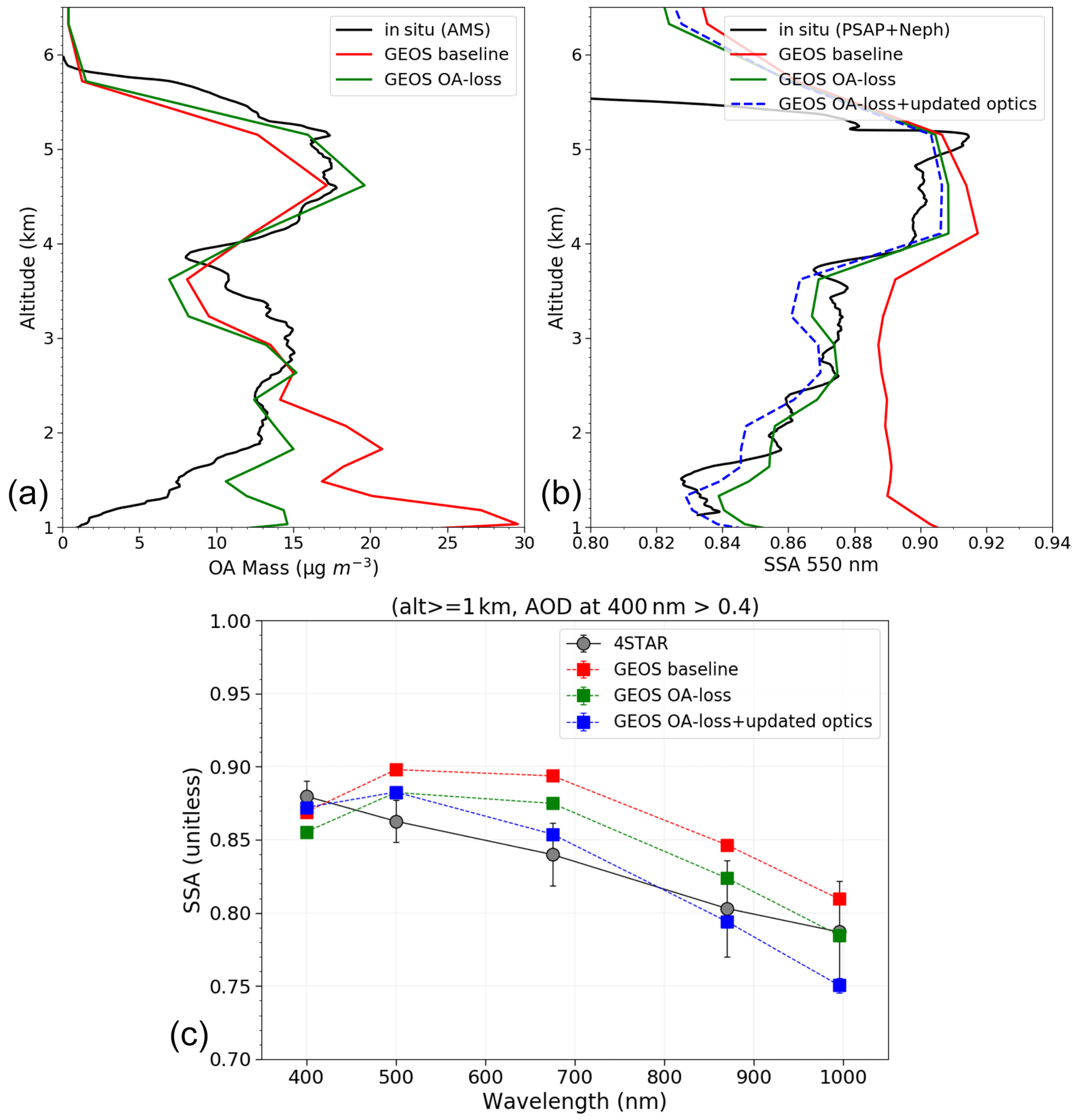
Figure 11 Model agreement across different observational spaces for the 24 September case: GEOS model-simulated (a) OA mass compared to AMS in situ measurements, (b) dry SSA profile compared to in situ (PSAP + nephelometer) measurements, and (c) spectral column SSA compared to 4STAR retrievals averaged over three locations depicted by blue stars in Fig. 3.

Table 3 Comparison of the observed and modeled mean SSA between 4STAR and GEOS experiments at 400, 500, and 675 nm.

3.2 Updated optics: adjusting OA Size distribution, hygroscopicity, and absorption

The previous section focused on the simulation of the aerosol lifecycle and mass distributions with emphasis on the profile flown on 24 September 2016. Here we broaden our use of the ORACLES dataset to better constrain the simulation of optical properties. As briefly described in Sect. 2.4, the model-derived aerosol optical properties (e.g., extinction coefficients, SSA, and phase function) for each aerosol component depends on the assumptions of their microphysical (size distribution, refractive index, etc.) and hygroscopic (or water uptake) properties. Therefore, we use the ORACLES dataset to first evaluate and then adjust three key model assumptions in this regard to improve the model agreement with the observations. Since OA contributes to about 60 %–70 % of the smoke plume mass observed during ORACLES (Fig. 6), only the particle properties of biomass burning OA and brown carbon component in the model were adjusted.

The first adjustment was made with respect to the particle size distribution. Within GOCART, a single-mode lognormal size distribution for the OA component is assumed, defined by a number mode radius (r_n) and geometric standard deviation (σ). The baseline model assumption for OA number size distribution (Fig. 12, red dashed line) shows a r_n=0.021 µm and σ=2.2 based on Chin et al. (2002). The comparison with UHSAS-measured particle size distribution for the available flight days shows that the observed particle size distribution (for accumulation mode) has a larger mode radius and narrower distribution than the model baseline assumption and does not show much variation amongst different flight days. Nonetheless, we limit the observations to the altitudes between 1–5 km and OA concentrations greater than 4 mg m⁻³ to ensure the presence of smoke particles. Therefore, for the updated optics case, we fit a lognormal distribution to the UHSAS-measured size distributions with a r_n=0.09 µm and σ=1.5 (Fig. 12).

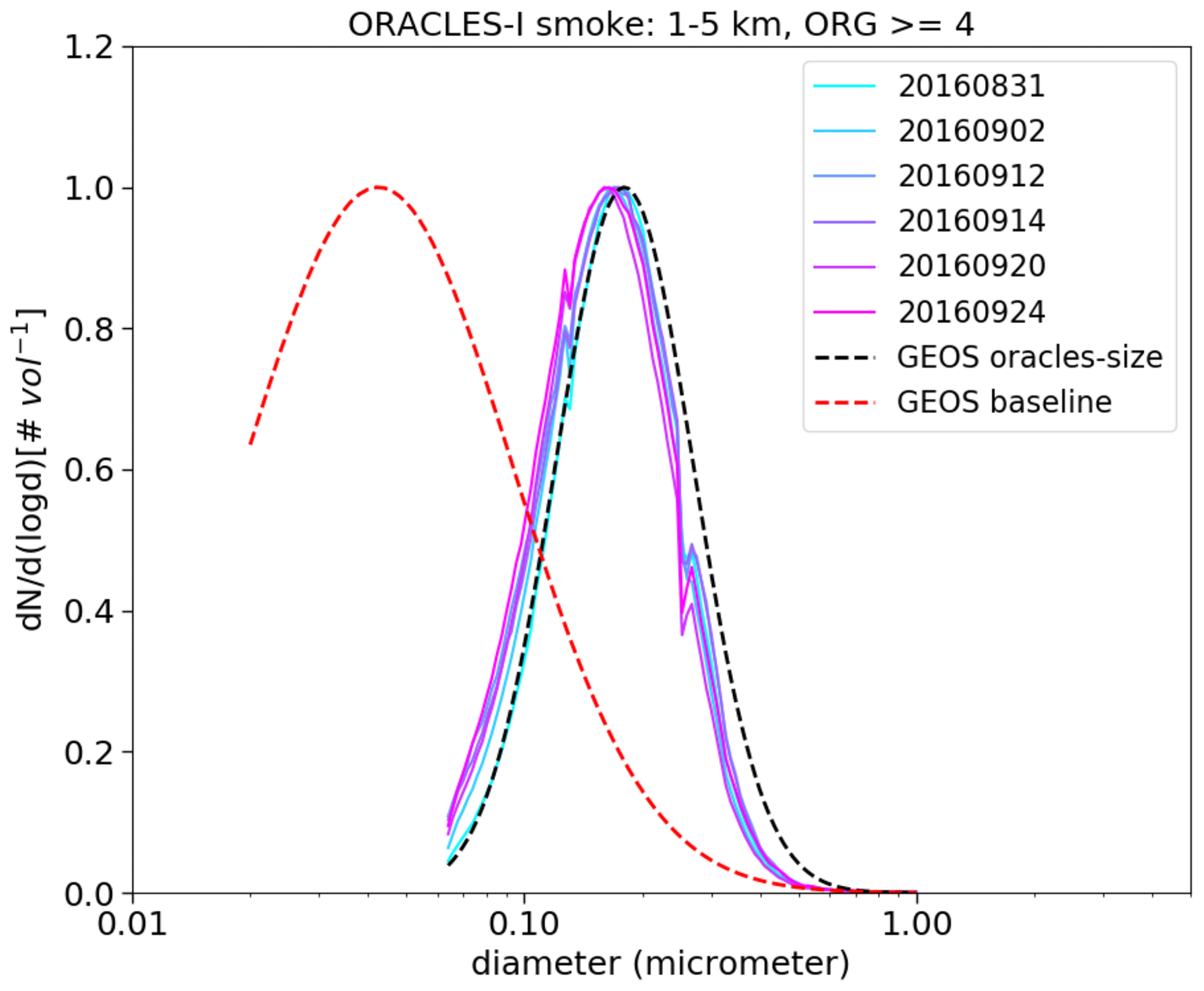
Figure 12 Comparison of GEOS baseline and adjusted particle size distribution for organic aerosol to ORACLES observations from the UHSAS instrument.

The second change is related to the model assumption of particle hygroscopicity. We utilized the dry and humidified nephelometer-measured scattering coefficients during ORACLES-I to obtain the scattering enhancement factor, f(RH). The f(RH) is defined as the particle light scattering coefficient at elevated RH divided by its dry value. We consider 80 % and 10 % as the high and low RH, respectively, and hence consider only those measurements that were obtained closest to these RH values before comparing with the model-derived f(RH) values at the same flight location (Fig. 13a). Additionally, to ensure the presence of smoke plumes, we only consider measurements that were made between 1.5–6 km altitude levels. Figure 13a shows that the GEOS baseline case significantly overestimates the observed f(RH) by almost a factor of 2. This model overestimation in f(RH) has also been previously reported in multi-model evaluation studies of Doherty et al. (2022) using the ORACLES dataset itself and in Burgos et al. (2020) using a global dataset of surface-based in situ measurements. Note that the modeled f(RH) presented here has contributions from a combination of smoke aerosol species. For GOCART, except for dust, all aerosol components are considered to have different degrees of hygroscopic growth rate with ambient moisture. We show the hygroscopic growth assumption for three major smoke aerosol components (organics, black carbon, and sulfate) in Fig. 13b based on the default optics table used within GOCART. Sulfate hygroscopic growth factor increases most rapidly with increasing RH, followed by organics and least rapidly for black carbon. Therefore, for the OA-loss model case (Sect. 3.1.3), where relative contribution of BC is enhanced for the aged plumes compared to OA, we see a slight reduction in modeled f(RH) compared to observations (Fig. 13a). An additional but minor reduction in modeled f(RH) is observed when the above-mentioned particle size distribution adjustments are made for the organic aerosol component in the model. Finally, we consider that the hygroscopic growth of OA is the same as for BC, and here we see the closest match to observations (a reduction of the simulated f(RH) from greater than 2 to about 1.7, compared to the value of 1.4 determined from the observations; see Fig. 13a and also the reduced ratio of the simulated-to-observed f(RH)), and thus this comprises our second adjustment to model assumption of OA properties.

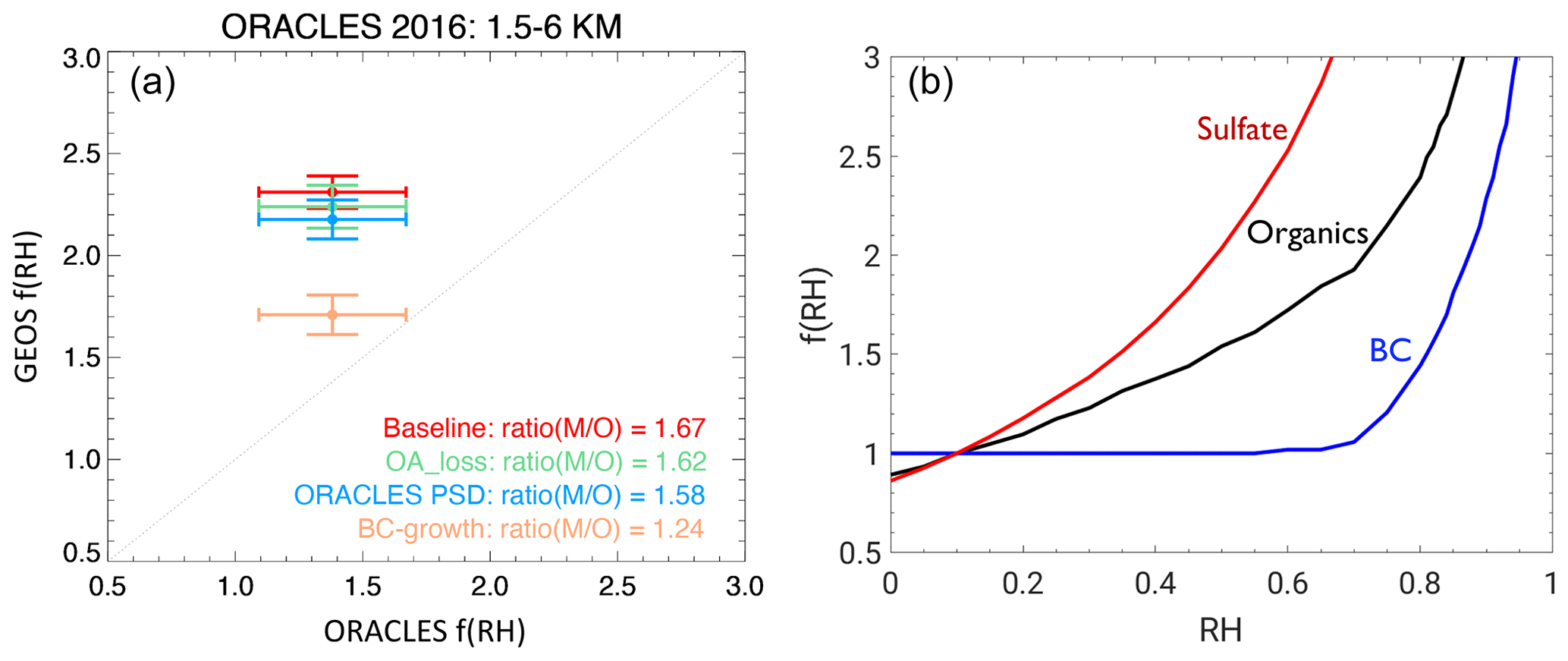
Figure 13 (a) Comparison of simulated to observed f(RH) in smoke plumes during the ORACLES-I deployment. Different cases of the model optical property assumptions are shown, and the ratio(M $/$ O) reports the ratio of the model to the observed mean values. (b) Default f(RH) in the GEOS lookup tables for sulfate, OA, and BC.

The third and final adjustment to the model optical properties is related to aerosol absorption, which is mainly characterized by the imaginary part of the complex refractive index (k) of the aerosol component. This change was motivated by our finding that our model-derived lidar ratios (i.e., the ratio of extinction to backscatter) of the smoke plumes were much higher than the observed values based on HSRL-2 measurements from the ER-2, especially in the 355 nm channel (70 sr versus 85 sr) for the model baseline case (Fig. 14a). A previous study by Veselovskii et al. (2020) that used the Raman Lidar observations over Senegal in West Africa for their analysis, also found that the GEOS modeled lidar ratios were consistently higher compared to their lidar observations for a range of relative humidity, when the model k in the UV was set to its baseline value (of k₃₅₀∼0.05). The aerosol backscattering coefficient is more sensitive to the absorption than the extinction coefficient because an increase in absorption is accompanied by a decrease in scattering. Thus, we expect that decreased absorption of OA in the UV should lead to a decrease in the lidar ratio. Figure 14 demonstrates the sensitivity of the lidar ratios to the changes in the imaginary component of the refractive index. The baseline optics table assumes $k_{\mathrm{350}}=\sim \mathrm{0.05}$, and so clearly reducing k₃₅₀ to 0.01 or 0.02 provides a better match of the model lidar ratio with the HSRL-2 observations (Fig. 14a). Note that we preserve the spectral contrast for all wavelengths <550 nm, so our adjustment of k₃₅₀ also implies a change at the longer wavelengths; hence, we simulate a different lidar ratio at 532 nm (Fig. 14b). For our final set of optics, we chose k₃₅₀=0.02 to have a reasonable simulation of the OMI AI values that we discuss later in Sect. 3.4.2.

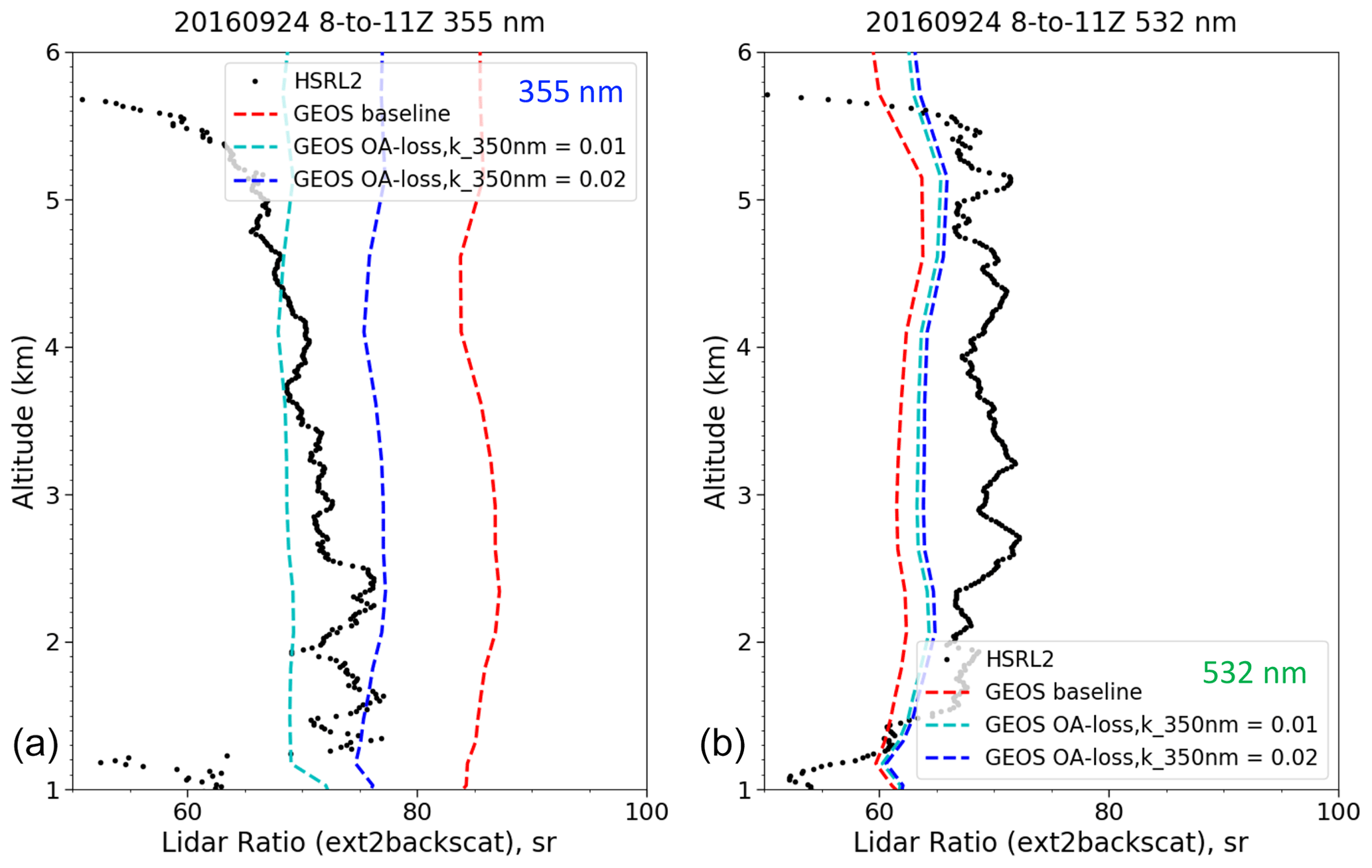
Figure 14 Comparison of the simulated and HSRL-2 observed lidar ratios at (a) 355 nm and (b) 532 nm for the profile near 12° S and 11° E on 24 September 2016.

A new optics table was generated following the above three changes in assumptions of OA microphysical and water uptake properties that we call “updated optics” throughout our figures and text. Now, we can revisit Fig. 11b and c to understand the impact of this optics update on the model-simulated SSA comparisons with the in situ and 4STAR observations. For the in situ profile at 550 nm, there is a small decrease in model SSA with “OA-loss + updated optics” compared to the OA-loss case (<0.01), and it remains within 0.02 of the observed SSA value at all altitudes (Fig. 11b). Figure 11c is better at showing the impact of these changes on the broader spectral curve. The “updated optics” case is less absorbing in the shortest 400 nm channel but otherwise more absorbing than both the baseline and “OA-loss with default optics” case. The former is expected due to the reduced OA absorption in near UV, and the latter is possibly due to the reduced hygroscopic growth assumptions that are leading to the formation of effectively smaller particles at enhanced RH within the smoke plumes. However, overall, the OA-loss + updated optics case shows the best agreement with the 4STAR observations compared to the other two cases for wavelengths less than 700 nm (Table 3). At longer wavelengths the improvement is less clear; although OA-loss + updated optics is closest to the 4STAR observations at 870 nm of all of our experiments, it shows the worst agreement at 1000 nm. We did not investigate other aerosol components (e.g., dust) that could contribute to especially long wavelength impacts. Note that the results in Fig. 11c are the average of three 4STAR retrievals on 24 September 2016 (Fig. 3), but similar SSA magnitudes and spectral curve shape, both for 4STAR and the different model simulations, hold when we average across all days of the ORACLES-I campaign (not shown here).

3.3 AOD and SSA evaluation at near-source AERONET sites

We evaluated the model performance of AOD and SSA at all the AERONET sites depicted in Fig. 1a. For brevity, we present here the comparative results from two key near-source sites, Mongu_Inn and Lubango, that had data availability for most days of September 2016 and are most contrasting in terms of the model performance. The model shows good agreement with AERONET observations over Lubango in terms of both AOD and SSA, and the final OA-loss + updated optics case has overall similar performance to the model baseline case (Fig. 15a, c) and improves the SSA simulation at 440 and 675 nm (Table 4). At Mongu_Inn, on the other hand, the model appears to have a systematic low AOD bias compared to AERONET observations but nonetheless can capture its daily variability (Fig. 15b). For SSA at Mongu (Fig. 15d), the model largely overestimates the absorption at longer wavelengths, and this together with AOD underestimation suggests that the model is likely missing a contribution from coarse-mode particles over this site. However, the model “OA-loss + updated optics” case, with its adjusted absorption at short wavelengths, results in a simulation in better agreement with the AERONET retrieved SSA at 440 nm.

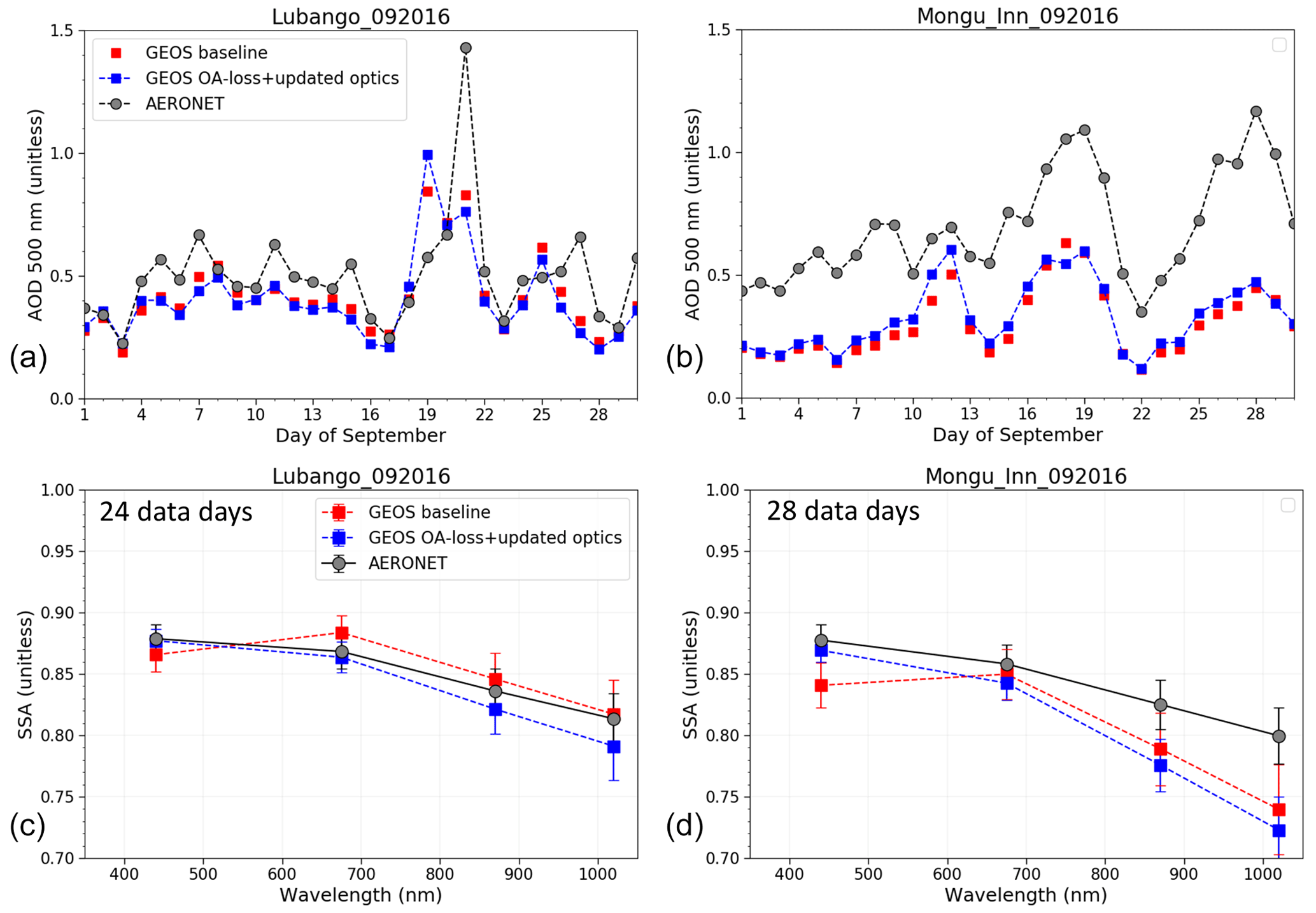
Figure 15 Comparisons of simulated and AERONET retrieved daily AOD at (a) Lubango and (b) Mongu_Inn sites over the continent for September 2016. The corresponding monthly mean spectral SSA are also compared between model simulations and AERONET (c) over Lubango and (d) Mongu_Inn, respectively.

Table 4 Comparison of the AERONET and GEOS SSA at two AERONET locations during September 2016.

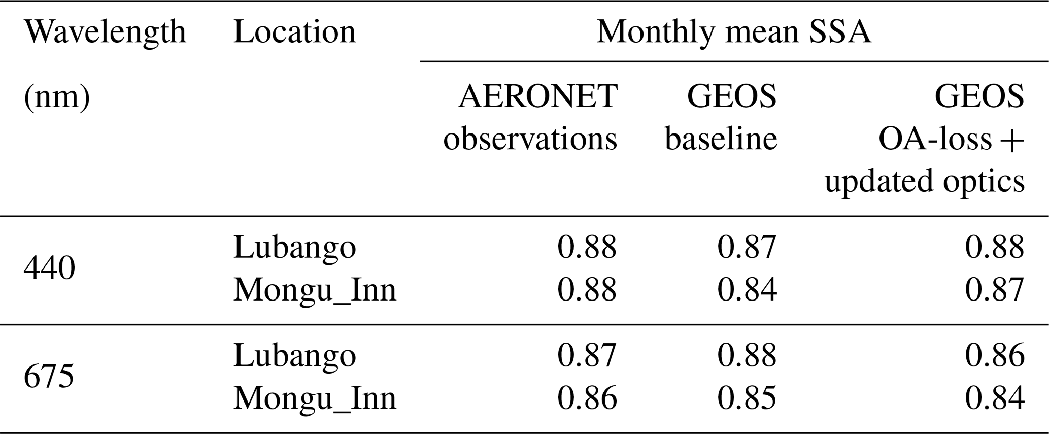
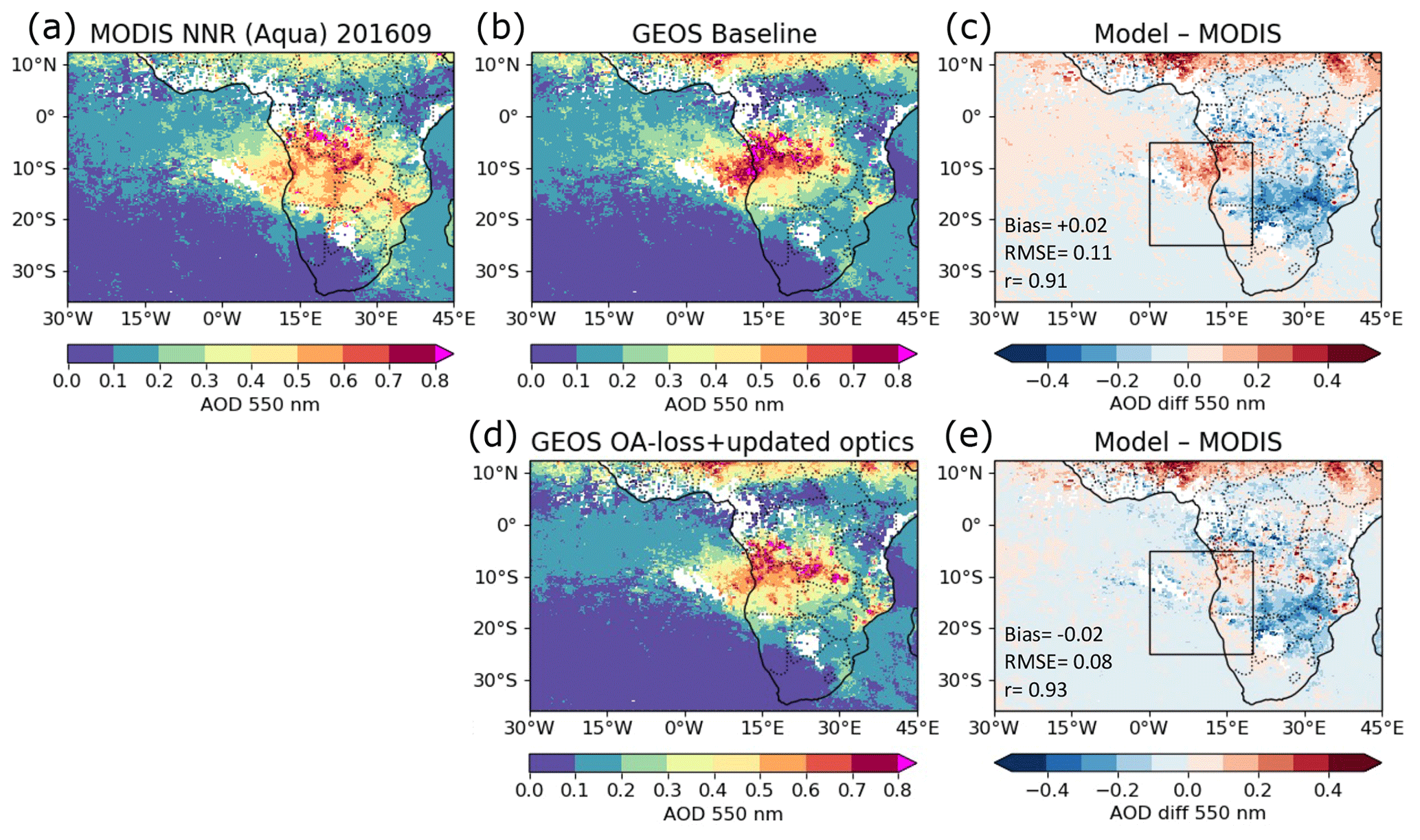
Figure 16 Comparisons of monthly mean AOD from (a) MODIS (Aqua) NNR retrievals and (b) GEOS baseline and (d) GEOS OA-loss+updated optics simulations. The corresponding AOD differences between the model simulations and MODIS observations are depicted in panels (c) and (e), respectively, along with the model performance metrics (mean bias, root-mean-square error, and Pearson correlation coefficient) for the region within the black box.

3.4 Satellite perspective: impact of updated optics on AOD and AI

3.4.1 Comparisons with MODIS NNR AOD retrievals

Satellite-based observations are used in this section to assess the model performance over the broader SE Atlantic and the source region over southern and central Africa. Figure 16a shows the September 2016 monthly mean MODIS NNR AOD. We sample the model AOD based on the MODIS swath, overpass time, and data availability, and the resulting monthly mean AOD from the model baseline and the final “OA-loss + updated optics” simulations are shown in Fig. 16b, d, respectively. The last column (Fig. 16c, e) shows the differences between the model and the observations. Broadly, as depicted in the AOD difference plots, both model simulations show a good agreement with the NNR retrievals, especially over the ocean and the smoke outflow region compared to the source region over the continent. There is a significant underestimation in terms of model AOD over the southeastern parts of the continent that persists in both the model simulations. This is a shortcoming of the GEOS model that has persisted in previous model versions as well, possibly due to missing biomass burning or coarse-mode aerosol sources (Das et al., 2017). Otherwise, there is a high bias in the model AOD in the areas around the western coast and 10° S in the baseline simulation (Fig. 16c). In our final simulation, however, this high bias in model AOD is reduced from +0.02 to −0.02 (Fig. 16d, e). Closer to the burning sources over land, this decrease in model AOD in our final simulation is due to the adjusted hygroscopic growth for the OA particles (see Sect. 3.2), whereas over the ocean, as the plumes move away from the continental burning sources, the decrease in model AOD is due to the accounting of OA loss with increasing smoke age. Finally, we also present the performance metrics (mean bias; root-mean-square error, RMSE; and Pearson correlation coefficient, r) to quantify the agreement between the model simulations and the observations with a focus over the ORACLES-I region (Fig. 16c, e). The statistical comparisons further emphasize that inclusion of OA loss processes and adjustments to model OA optics does not deteriorate the model performance in terms of AOD simulation, but that it instead makes it marginally better compared to baseline run by lowering the RMSE (from 0.11 to 0.08) and increasing the r values (from 0.91 to 0.93). Note that we chose to show only the Aqua MODIS results here since Aqua has a closer overpass time with OMI (Aura) than Terra, but the comparisons of model AOD simulations with respect to Terra MODIS retrievals (not shown here) also showed similar results.

3.4.2 Comparisons with OMI AI observations

In Fig. 17 we show the GEOS-simulated OMI AI for September 2016 in comparison to the OMI retrievals. The OMI retrieved AI is shown in Fig. 17a. To minimize the impact of clouds on the comparison we retain only OMI pixels with QA values of 0 (low probability of cloud contamination). For the model-calculated AI, the GEOS-simulated aerosol profiles are sampled at the OMI footprints. The model optical property assumptions are applied to the simulated aerosol profiles, and with the OMI observation geometry and retrieved surface reflectance they are input to the AI calculator, which simulates the OMI radiances. The simulated radiances only include terms for the aerosol, molecular background, and surface.

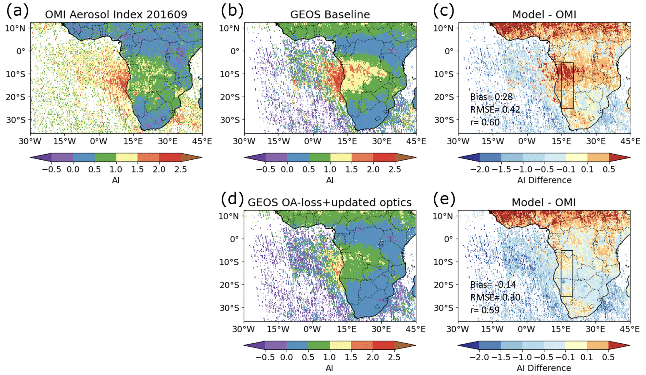
Figure 17 The September 2016 average OMI-retrieved AI (a) and the simulated GEOS AI for the baseline (b) and OA loss+updated optics (d) model runs. The GEOS–OMI difference is shown compared to the GEOS baseline run (c) and the OA loss + updated optics runs (e), respectively, along with the model performance metrics (mean bias, RMSE, and r) for the region within the black box.

Two cases are shown in the comparison: the GEOS baseline run (Fig. 17b) and the final run that includes OA loss with smoke age, increased biomass burning emissions, and ORACLES-informed optical properties for OA (OA-loss + updated optics, Fig. 17d). The baseline run, with its more highly absorbing OA assumptions and high bias in aerosol loading especially near the coast of southwestern Africa (10° S, Fig. 16c), results in the model overestimating the AI relative to OMI, with this high bias especially apparent over both land and ocean where the AOD was overestimated in the model (Fig. 17c). By contrast, the GEOS model run with the ORACLES-informed adjustment to the optical property assumptions, along with the reduced overall burden of OA, results in a much more favorable comparison of the simulated to retrieved AI (Fig. 17e). The apparent discontinuity in the AI magnitude between land and sea along the western coast of southern Africa is a sampling artifact brought on by cloud screening, with nearly 3× as many OMI pixels retained over land as for over the coastal ocean. For this reason, we restrict a quantitative assessment of the model performance to the boxed region over land shown in Fig. 17c, e, and statistics are also reported in Fig. 17. In the indicated region there is an improvement in the bias of the modeled AI from +0.28 to −0.14 and a reduction in the RMSE from 0.42 to 0.30 in moving to the updated aerosol optics. This improvement and our assessment of the model performance with the independent OMI dataset shows the overall consistency between the optical properties that were derived in situ from the ORACLES measurements and what can be retrieved from space-based remote sensing, with the GEOS model as the interpolator between the two datasets.

3.5 Radiative implications

Finally, we consider the impact of the updated aerosol simulation on the modeled direct radiative forcing of the aerosols, which along with any possible aerosol–cloud interactions drive the aerosol impacts on climate. Figure 18a shows the September 2016 monthly mean 550 nm AOD difference between the GEOS baseline and updated (OA-loss + updated optics) model runs. The difference is consistent with the results in Fig. 16 and shows that the enhanced biomass burning emissions in the updated run result in a slightly higher AOD over southeastern Africa, while the inclusion of the OA loss process in the updated run leads to somewhat less aerosol downwind and an overall lower smoke AOD over the southeastern Atlantic compared to the baseline (i.e., the baseline run has a higher AOD over the ocean). Clouds are not much changed between the two model runs, so in Fig. 18b we show the low-cloud fraction from the baseline run, which shows a main cloud feature (cloud fraction >40 %) centered at 10°–15° N extending west of the continent.

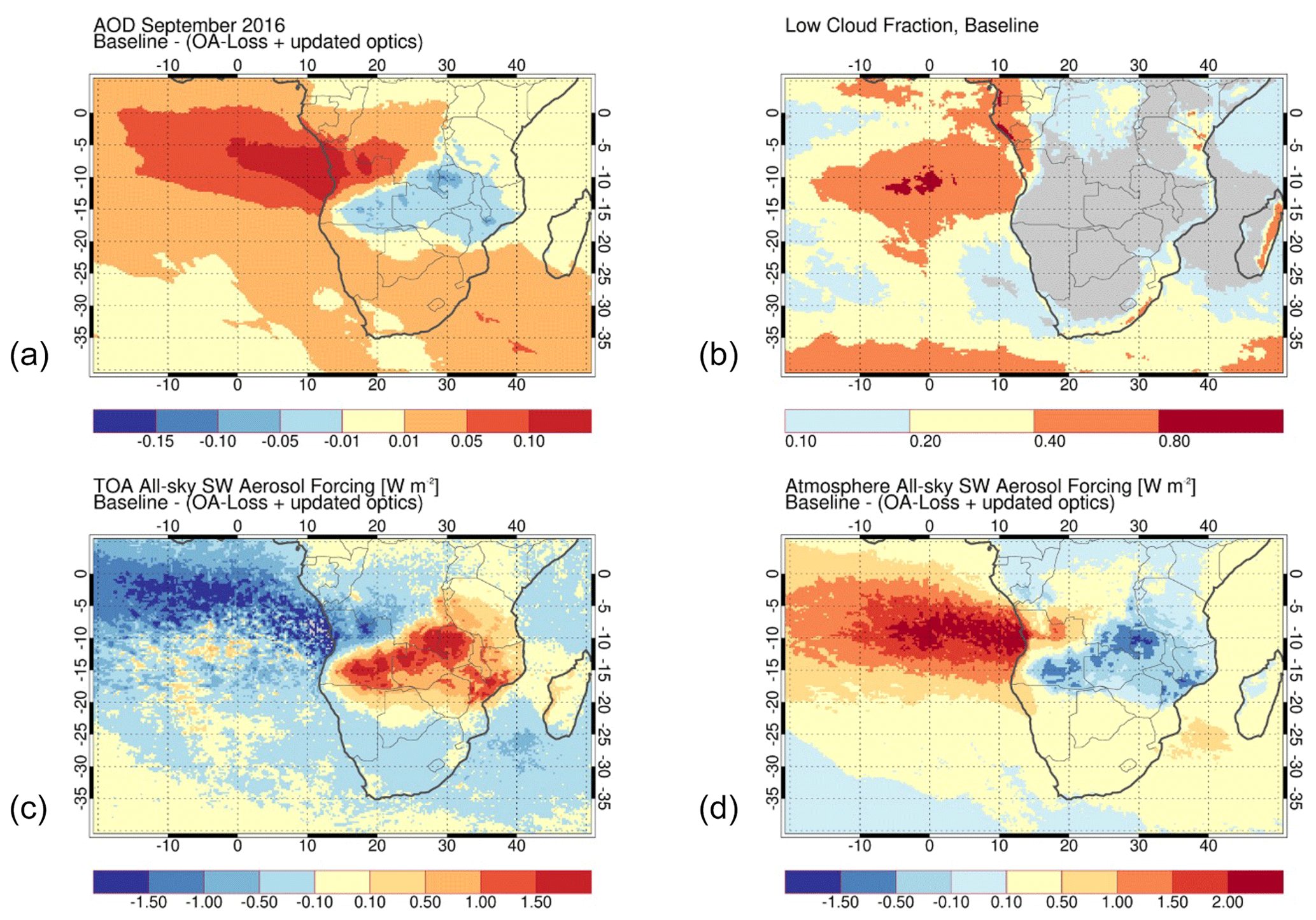
Figure 18 The September 2016 average GEOS-simulated (a) total 550 nm AOD difference between the baseline and OA-loss + updated optics model runs, (b) the low-cloud fraction of the baseline run, (c) top-of-atmosphere all-sky shortwave aerosol forcing difference of the baseline and updated runs, and (d) the all-sky shortwave aerosol atmospheric heating difference of the baseline and updated runs. The grey area in (b) is cloud fraction less than 10 %.

Figure 18c shows the TOA all-sky shortwave (SW) radiative forcing due to aerosol, presented as a difference between our two runs. For each model run, the radiative forcing is computed by two successive calls to the radiative transfer code, one including the effects of aerosols and the other without the aerosols. The aerosol forcing is defined as the difference between the net TOA radiation with aerosols minus the net TOA radiation without aerosols (i.e., SW_{net_aer} – SW_{net_noaer}) and represent an increase (positive) or decrease (negative) of energy. There is an overall ∼1 W m⁻² difference in the SW forcing over the southeastern Atlantic on the northern edge of the smoke plume. This difference is on the margins of the smoke plume to the north of the main cloud features (Fig. 18b) and has a negative magnitude as defined because in the baseline simulation there is more (relatively cooling) aerosol over the darker ocean surface and thus more radiation reflected to space. The broad positive SW forcing difference over the continent reflects the relatively greater backscattered solar radiation over the dark continental surface corresponding to the higher AOD in that region in the updated model run (region of over-land negative AOD difference in Fig. 18a).

Finally, Fig. 18d shows the SW atmospheric heating due to aerosols in the two model runs. This is the difference in the net forcing at TOA and at the surface. That enhanced loading (Fig. 18a) and the relatively more absorbing optics of the baseline suggest a greater warming of the atmosphere versus the updated run, which would tend to stabilize the atmosphere. By contrast, our updated simulation has somewhat less atmospheric warming over the regional cloud decks.

4 Conclusions and future directions

In this study, we utilized the detailed ORACLES-I aircraft observations to evaluate the current state of biomass burning aerosol properties and transport in the NASA GEOS model following recent developments in its representation of carbonaceous aerosols. An example case study of 24 September was analyzed in detail, during which in situ and remote sensing observations showed a presence of multi-layered smoke plume structure with significantly varying SSA in the vertical. Our baseline simulations were not able to represent the observed OA : BC ratio or the vertically varying single-scattering albedo. Analyzing the simulated smoke age suggests that the higher-altitude, less absorbing smoke in the plume was younger (∼4 d), while the lower-altitude, more absorbing smoke plume was older (∼7 d). We hypothesize a loss process – chemical or microphysical – to explain the change in aerosol absorption as the smoke plume ages, and we apply a simple 6 d e-folding loss rate to the hydrophilic biomass burning OA to simulate this process. Adding this loss channel requires some adjustment to the assumed aerosol emissions to approximately conserve the regional aerosol loading and further improve the simulated OA : BC ratio, and we have accordingly increased our biomass burning emissions of OA by 60 % and biomass burning BC emissions by 15 %. Next, we use the aircraft-based observations to better constrain the simulation of aerosol optical properties. For the biomass burning OA aerosol component within GEOS, we adjust the lognormal size distribution to have a modal radius, r_n=0.09 µm and σ=1.5, based on the ORACLES-I HiGEAR (or UHSAS) observations. Secondly, the OA hygroscopic growth is assumed to increase less rapidly with increasing RH compared to default assumptions and simulate the hygroscopic growth rate of model BC, which provides a simulated f(RH) similar to the observed. Finally, we also adjusted the OA complex refractive index (k₃₅₀=0.02) to reduce the OA absorption in the near UV to match better with the HSRL-2 retrieved lidar ratio and OMI retrieved AI. Our final GEOS model simulation with additional OA loss and updated optics showed a better performance in simulating AOD and SSA compared to independent AERONET observations and MODIS NNR AOD retrievals for the entire month of September 2016. In terms of radiative implications of our model adjustments, the final GEOS simulation suggests a decreased atmospheric warming of ∼2 W m⁻² over the southeastern Atlantic region and above the stratocumulus cloud decks compared to the model baseline simulations.

The simplistic approach presented in this study to address the microphysical or chemical loss of OA with increasing smoke age lacks a specific physical basis. In subsequent modeling studies, the mechanisms causing this OA loss can be further explored, and if the OA loss is indeed associated with continued oxidation of OA during the aging of smoke, the loss can be parameterized as a function of oxidant fields in the model rather than assuming a single e-folding time to simulate the aerosol loss. Moreover, observations over other major biomass burning regions of the globe need to be analyzed to find if a similar variation in SSA is observed for aging plumes in those regions and a global parameterization for OA loss will need to be explored. Finally, we will also need to utilize the observations from subsequent years of ORACLES (i.e., 2017 and 2018) to confirm whether the suggested set of OA microphysical and hygroscopic assumptions in the model for the 2016 case are also able to capture the seasonal variability of smoke emissions in this region.