the Creative Commons Attribution 4.0 License.
the Creative Commons Attribution 4.0 License.
 | 09 Apr 2024
Atmospheric oxygen as a tracer for fossil fuel carbon dioxide: a sensitivity study in the UK
Hannah Chawner
Karina E. Adcock
Tim Arnold
Yuri Artioli
Caroline Dylag
Grant L. Forster
Anita Ganesan
Heather Graven
Gennadi Lessin
Peter Levy
Ingrid T. Luijkx
Alistair Manning
Penelope A. Pickers
Chris Rennick
Christian Rödenbeck
We investigate the use of atmospheric oxygen (O2) and carbon dioxide (CO2) measurements for the estimation of the fossil fuel component of atmospheric CO2 in the UK. Atmospheric potential oxygen (APO) – a tracer that combines O2 and CO2, minimizing the influence of terrestrial biosphere fluxes – is simulated at three sites in the UK, two of which make APO measurements. We present a set of model experiments that estimate the sensitivity of APO simulations to key inputs: fluxes from the ocean, fossil fuel flux magnitude and distribution, the APO baseline, and the exchange ratio of O2 to CO2 fluxes from fossil fuel combustion and the terrestrial biosphere. To estimate the influence of uncertainties in ocean fluxes, we compare three ocean O2 flux estimates from the NEMO–ERSEM, the ECCO–Darwin ocean model, and the Jena CarboScope (JC) APO inversion. The sensitivity of APO to fossil fuel emission magnitudes and to terrestrial biosphere and fossil fuel exchange ratios is investigated through Monte Carlo sampling within literature uncertainty ranges and by comparing different inventory estimates. We focus our model–data analysis on the year 2015 as ocean fluxes are not available for later years. As APO measurements are only available for one UK site at this time, our analysis focuses on the Weybourne station. Model–data comparisons for two additional UK sites (Heathfield and Ridge Hill) in 2021, using ocean flux climatologies, are presented in the Supplement. Of the factors that could potentially compromise simulated APO-derived fossil fuel CO2 (ffCO2) estimates, we find that the ocean O2 flux estimate has the largest overall influence at the three sites in the UK. At times, this influence is comparable in magnitude to the contribution of simulated fossil fuel CO2 to simulated APO. We find that simulations using different ocean fluxes differ from each other substantially. No single model estimate, or a model estimate that assumed zero ocean flux, provided a significantly closer fit than any other. Furthermore, the uncertainty in the ocean contribution to APO could lead to uncertainty in defining an appropriate regional background from the data. Our findings suggest that the contribution of non-terrestrial sources needs to be better accounted for in model simulations of APO in the UK to reduce the potential influence on inferred fossil fuel CO2 using APO.
- Article
(7463 KB) - Full-text XML
-
Supplement
(10483 KB) - BibTeX
- EndNote


Variations in atmospheric carbon dioxide (CO2) concentrations are due to atmospheric transport and the influence of fluxes from the terrestrial biosphere, the ocean, and human activities. With the ultimate aim of evaluating national emission estimates, a major goal of several recent studies has been the isolation of only those variations due to anthropogenic fossil fuel CO2 (ffCO2) emissions. Radiocarbon (14C) has been widely used as a tracer for this purpose (e.g. Levin et al., 2003; Graven et al., 2009, 2018; Wenger et al., 2019; Zazzeri et al., 2023). As fossil fuel emissions are depleted in 14C, they can be distinguished from biospheric and oceanic processes. However, atmospheric 14C measurements are expensive, they cannot be made continuously to the required precision, and in some regions there may be a significant interference of 14C emissions from gas-cooled nuclear power stations (Graven and Gruber, 2011; Bozhinova et al., 2016; Wenger et al., 2019). An alternative tracer is carbon monoxide (CO), which is produced by incomplete combustion. Atmospheric measurements of CO are much less expensive than those of 14C and can be made continuously (e.g. Andrews et al., 2014; Levin and Karstens, 2007; Levin et al., 2020). However, there is large uncertainty in both the ratio of CO to CO2 emissions from fossil fuel combustion and the CO flux from non-fossil-fuel sources and sinks (Vardag et al., 2015).
Pickers (2016) and Pickers et al. (2022) show that atmospheric oxygen (O2) and CO2 measurements, combined into atmospheric potential oxygen (APO) (Stephens et al., 1998), can be used as a novel tracer for fossil-fuel-derived CO2. In their study, Pickers et al. (2022) show that their APO-derived CO2 emission changes during the COVID-19 lockdowns in the UK correspond well to the changes found from bottom-up inventories. Their method, combining observations and machine-learning techniques, shows the potential of APO as a fossil fuel CO2 tracer. The basis of this method is that the ratio of O2 to CO2 fluxes from the terrestrial biosphere, which are by definition removed from the O2 signal through the use of the APO tracer (Stephens et al., 1998), is relatively well-constrained and invariant in space and time. For land-based sources, O2 and CO2 fluxes to the atmosphere from photosynthesis, respiration, and combustion are strongly anti-correlated: CO2 is taken up through photosynthesis whilst O2 is released, and the reverse is true for respiration and combustion.
When considering ocean fluxes, the situation is more complex. Differences in solubility (Keeling, 1988b) and carbonate chemistry (Keeling and Shertz, 1992; Keeling and Severinghaus, 2000) mean that O2 and CO2 fluxes from the ocean are largely decoupled. However, previous work has indicated that the influence of ocean fluxes on the atmospheric ratio of O2 to CO2 is generally smaller than the influence of fossil fuel combustion on short timescales (Pickers, 2016; Pickers et al., 2017; Chevalier and WP4 CHE partners, 2021). Pickers et al. (2017) found short-term variability in APO, O2, and CO2 mole fractions with a very small magnitude from the ocean when taking ship measurements.
There have been a number of promising attempts to incorporate O2 modelling as a tracer for ffCO2. Kuijpers (2018) modelled O2 for the autumn of 2014, finding good agreement with observations at two sites in the UK and the Netherlands. APO modelling was investigated to derive European ffCO2 fluxes by several groups within the CO2 Human Emissions project (CHE, work package 4; Marshall et al., 2019; Chevalier and WP4 CHE partners, 2021). Comparing with results from Δ14CO2 (∼ ) and CO modelling, they found that APO-derived ffCO2 gave the strongest correlation to direct ffCO2 models using STILT (Stochastic Time-Inverted Lagrangian Transport model) and TNO fluxes. The APO models were affected by oceanic fluxes at some coastal sites, although for most coastal sites the ocean influence, modelled using ocean fluxes from NEMO–PlankTOM5, was considerably smaller than ffCO2.
Two measurement sites equipped with high-frequency CO2 and O2 instruments have been established in the UK: one at the Weybourne Atmospheric Observatory (WAO) in the east of England and one at Heathfield (HFD) telecommunications tower in the south of England. In this paper, we perform simulations of CO2 and O2, primarily focusing on model–data comparisons at WAO for the year 2015, with further comparisons at HFD and WAO for the year 2021 presented in the Supplement along with a third station at Ridge Hill (RGL) telecommunications tower. Although atmospheric O2 measurements are not available from RGL, it is included to examine the modelled APO further inland. We test the sensitivity of the APO simulations to changes in a set of uncertain model input parameters to determine whether a robust tracer of national scale fossil fuel CO2 can be derived.
Modelling atmospheric potential oxygen
As O2 is abundant in the atmosphere, dilution by trace gases can have a non-negligible effect on its mole fraction, which may erroneously be attributed to an O2 flux. To minimize this influence, atmospheric oxygen mole fraction measurements are commonly reported as a ratio with respect to the atmospheric nitrogen mole fraction as (Keeling and Shertz, 1992):
where is the ratio of a sample and is from a reference gas cylinder. is expressed in “per meg”.
We can define the tracer APO (e.g. Stephens et al., 1998; Gruber et al., 2001; Battle et al., 2006), which is largely unaffected by exchanges with the terrestrial biosphere but sensitive to fossil fuel (and cement production) and ocean fluxes. This is a weighted combination of O2 and CO2 which isolates the oceanic and fossil fuel (and cement production) components:
where APO is a mole fraction, αB is the O2 : CO2 exchange ratio for the land biosphere, O2 and CO2 are the atmospheric mole fractions of O2 and CO2 respectively, and 350 (µmol mol−1) is an arbitrary reference.
Equations (1) and (2) can be combined, expressing δAPO in per meg (Stephens et al., 1998):
where is the standard mole fraction of O2 in air, equal to 0.20946 (Machta and Hughes, 1970).
The regional contribution to APO
The regional contribution of APO can be estimated by combining the mole fraction contributions of O2, CO2, and N2. Following the derivation in Manning and Keeling (2006), baseline deviations of APO, expressed in per meg, can be written as
where Z and O respectively are the O2 and CO2 mole fraction contributions from the ocean; F and FO are the contributions of CO2 and O2 respectively from fossil fuel combustion and cement production; N is the N2 contribution; αF and αB are the fossil fuel and biospheric exchange ratios, respectively; and is the mole fraction of N2 in dry air, given as 0.78084 (Weast and Astle, 1982), where this and are used to convert from ppm (µmol mol−1) to per meg.
When estimating the exchange of N2 we need only to consider the ocean contribution, as the other components are assumed to be negligible (Ciais et al., 2007). We assume a constant value for αB for the UK of −1.07 ± 0.04 (Marshall et al., 2019; Penelope A. Pickers, personal communication, 2021). αF varies for different fuel types, having values of −1.17 for coal, −1.44 for oil, −1.95 for gas, and 0 for cement production (Keeling, 1988a; Steinbach et al., 2011), and can be estimated for the UK by combining fossil fuel emission estimates and fuel usage statistics, as outlined in Sect. 2.2.2. However, variations in αF are not well studied or well constrained. Therefore we follow Jones et al. (2021) in assuming an uncertainty of ±3 %.
2.1 Observations
At both measurement stations, WAO and HFD, atmospheric O2 measurements are taken using Oxzilla lead fuel cell analysers (Sable Systems International Inc.) placed in series with non-dispersive infrared (NDIR) ULTRAMAT 6E CO2 analysers (Siemens Corp.). The gas handling for each system is similar to that of Adcock et al. (2023), Pickers et al. (2017), and Stephens et al. (2007), to ensure stable pressures and flow rates are maintained and to avoid fractionation effects. A two-stage drying system (Wilson, 2013; Barningham, 2018; Adcock et al., 2023) reduces the dew point of the sample air to approximately −90 °C. Calibration gases, consisting of secondary standards that are stored horizontally in thermally insulated enclosures, are used to characterize analyser responses on the World Meteorological Organization (WMO) CO2 scale maintained by the National Oceanic and Atmospheric Administration (NOAA) and the Scripps Institution of Oceanography scale for O2 by employing routines and protocols similar to those of Kozlova and Manning (2009).
The Weybourne Atmospheric Observatory (WAO; https://weybourne.uea.ac.uk/, 13 March 2024) is a coastal measurement station in Norfolk, in the east of England (52°57′02′′ N, 1°07′19′′ E), which has been routinely sampling CO2 and O2 since May 2010. Established in 1992, the WAO is a Global Atmospheric Watch (GAW) regional station, a National Centre for Atmospheric Sciences (NCAS) Atmospheric Measurement Facility (AMF), and an Integrated Carbon Observation System (ICOS) Class 2 station. Air is alternately sampled from two identical aspirated inlets at 15 m a.g.l. (Blaine et al., 2006).
Heathfield is a tall tower measurement site that is part of the UK Deriving Emissions linked to Climate Change (DECC) network (Stanley et al., 2018) and has been sampling CO2 and O2 since June 2021. The site is in an agricultural area in the south of England (50°58′36.3′′ N, 0°13′49.728′′ E), about 25 km north of the English Channel. Air is alternately sampled from two identical aspirated inlets (Blaine et al., 2006) at 100 m a.g.l.
Ridge Hill is also a tall tower measurement site in the UK DECC network in Herefordshire (51°59′50.766′′ N, 2°32′23.64′′ W). Although CO2 is sampled here, O2 is not. We include Ridge Hill in the analysis to test the model at a more inland UK site.
The repeatability of the O2 measurements from Weybourne, which is determined from regular measurements of a target tank, typically ranges from 1.68±1.09 per meg to 3.31±5.46 per meg (Adcock et al., 2023). This exceeds WMO repeatability goals (WMO, 2019) for O2 and is amongst the most precise globally. The repeatability is calculated using the method described in Pickers et al. (2017) and is reported with ±1σ uncertainty to represent how the measurement system repeatability varies over time. During the period February to November 2015, the O2 measurement repeatability was significantly larger (10.71±10.45) than usual, caused by poor performance of the Oxzilla analyser. As described in Sect. 2.2, we model the year 2015, as it is the most recent year for which outputs exist for all of the ocean models used. This larger repeatability does not significantly affect the accuracy of the O2 measurements, but it does compromise the detection limit, meaning that smaller synoptic variations in APO (< 10–20 per meg) may be masked during this period by the measurement imprecision. CO2 repeatability was not affected and is 0.005±0.023 ppm on average at Weybourne, calculated from over 8000 target tank measurements made from 2010–2021.
2.2 Modelling APO
We use a Lagrangian particle dispersion model (LPDM) to simulate APO at the three measurement sites in the south of the UK. The key components of our simulation are the LPDM “footprints”, a set of flux estimates, and boundary conditions at the edge of our domain. The following sections outline how each component was produced and used in the model.
For our analysis we focus on the year 2015, chosen because time-resolved ocean model outputs are available for all ocean models considered here, described in Sect. 2.2.2. Weybourne measurements are available for 2015 and are compared to the simulations in Sect. 3. Heathfield observations are only available from June 2021, when time-resolved ocean fluxes are not available, so model outputs, derived using climatological fluxes, are compared to the observational data for this site and are shown in the Supplement. Simulations at Ridge Hill are shown in the Supplement.
We also model the total CO2 and O2 mole fractions at Weybourne to compare the correlations with those observations to the equivalent for APO.
2.2.1 The atmospheric model
Simulations of atmospheric transport and dispersion are carried out using the Numerical Atmospheric-dispersion Modelling Environment (NAME III, version 7.2), the UK Met Office's LPDM (Jones et al., 2007). NAME was run in time-reversed mode, in which we tracked thousands of model particles back in time for 30 d from measurement sites (see e.g. Manning et al., 2011). The motion of hypothetical “particles” is simulated based on meteorological fields from the Met Office Unified Model analyses (Cullen, 1993). The “footprint” of each measurement was estimated by recording locations and times at which particles interacted with the Earth's surface (defined as being the lowest 40 m of the atmosphere in this case). These footprints relate the sensitivity of mole fractions at a measurement site to the flux from each grid cell in the domain. Our domain covered most of Europe, the east coast of North and Central America, and northern Africa, extending across the longitude–latitude range: 10.729–79.057° N and 97.9° W–39.38° E (shown in Fig. S1 in the Supplement). The footprints have the resolution 0.234° by 0.352° (roughly 25 km by 25 km over the UK).
The NAME footprints used for this study are disaggregated in time with the method described by White et al. (2019). To account for the influence of rapid variations in CO2 flux on the mole fractions, footprints are generated hourly for the 24 h preceding a simulated data point. Time-integrated footprints are then used for the remaining 29 d of the simulation. The modelled regional contribution to the mole fraction of a species, Yt, at a time step, t, can then be estimated by combining the flux field with the high time resolution NAME footprint, as shown by Eq. (6) (White et al., 2019):
where H is the number of hours back in time over which the footprint is disaggregated, for which we use 24; h is the number of hours back in time before the particle release time, t; j is the grid cell; N is the maximum number of grid cells; is one grid cell of the footprint for that time; is one grid cell of the flux field; is the remaining 29 d footprint; and is the monthly average flux for the grid cell (by calendar month). White et al. (2019) discuss this method in more detail, including the effects of varying the level of time-disaggregation of the footprint, H.
2.2.2 Flux products
We model the regional contribution to APO separately for each of the components of Eq. (5) (Z, FO, F, O), using Eq. (6) to combine the flux estimates and NAME footprints. Here we describe how the fluxes for each component are estimated.
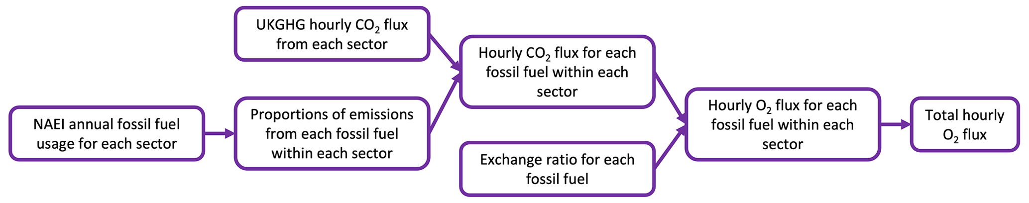
Anthropogenic CO2 flux estimates for the UK are taken from the UK National Atmospheric Emissions Inventory (NAEI), where estimates at a downscaled hourly resolution are derived using the UKGHG (UK Greenhouse Gas) model (Levy, 2020). Outside of the UK, anthropogenic flux estimates from EDGAR (Emissions Database for Global Atmospheric Research) are used. As the NAEI includes the anthropogenic CO2 flux estimates from both fossil fuel and non-fossil-fuel sources (e.g. peat and biomass), we use the method described in Fig. 1 and Equations (7) and (8) to remove emissions associated with non-fossil-fuel sources and thus estimate the UK fossil fuel CO2 and O2 flux:
where s is the SNAP (Selected Nomenclature for reporting of Air Pollutants, see e.g. Tsagatakis et al., 2022) sector, e is the fuel or source type (coal, oil, gas, non-combustion, or cement production), CO2s is the CO2 flux for the sector, Rse is the proportion of CO2 emissions within the SNAP sector associated with the fuel type, and αFe is the fossil fuel exchange ratio for the fuel type. We use NAEI statistics of the annual fuel usage for each SNAP sector (https://naei.beis.gov.uk/data/data-selector, last access: 13 March 2024) to determine Rse, assuming that the ratio of fuels used within each sector is constant throughout the year. When determining the fuel type associated with NAEI emission estimates we follow the assumptions given by Jones et al. (2021), that emissions from the non-energy use of fuels and the solvent sector relate to non-combustion use of oil, and emissions from the production of non-metallic minerals relate to cement clinker production. Using the exchange ratio for each fuel, αFe, we then convert from CO2 to O2 flux for each fuel within each sector and take the sum to give the total hourly O2 flux throughout the year. The O2 flux from outside of the UK is estimated using EDGAR CO2 fields and αF estimates from GridFED (Jones et al., 2021).
We compare ocean CO2 and O2 fluxes derived from NEMO–ERSEM simulations (NE; Butenschön et al., 2016; Madec and NEMO System Team, 2022), the ECCO–Darwin model (ED; Carroll et al., 2020), and the Jena CarboScope APO inversion (JC; Rödenbeck et al., 2008), as well as a model with ocean fluxes excluded. All of the ocean fluxes have daily time resolution and raw spatial resolutions of 0.199°×0.333°, 2.0°×2.5°, and 0.066°×0.110° for ED, JC, and NE respectively, which are regridded to match the NAME spatial resolution.
ED determines ocean–atmosphere transfer of O2 and CO2 by combining the CO2 partial pressure difference across the air-sea interface with the relationship between wind speed and gas transfer, as described by Wanninkhof (1992). The Darwin Project biogeochemical model resolves the cycling of CO2 and O2, and its ocean ecology includes phytoplankton and zooplankton (Brix et al., 2015; Carroll et al., 2020). JC estimates CO2 and APO fluxes using a Bayesian atmospheric inversion and measurements from 23 CO2 measurement stations and up to 10 O2 measurement stations (including Weybourne; Rödenbeck et al., 2014, 2008, 2018). For the JC APO inversion, oceanic CO2 fluxes are estimated from the interpolation of pCO2 data. Air–sea fluxes of O2 and CO2 in NE are calculated starting from the gradient of those gases between the atmosphere and the water and by using Nightingale et al. (2000) to estimate the gas transfer coefficient. The concentrations of O2 and CO2 in the water are the results of dynamical processes in the ecosystem represented in the model and, in particular, photosynthesis from phytoplankton and respiration of all planktonic communities, as well as benthic organisms. More details on the dynamics of these gases can be found in Butenschön et al. (2016). For all of our APO models we use a nitrogen flux field estimated from NEMO heat fluxes by Eq. (9):
where is the temperature derivative of the solubility, is the ocean heat flux (positive for transfer from the ocean to the atmosphere), and Cp is the heat capacity of seawater (Keeling et al., 1993). is estimated using
with
where C is the gas concentration, T is the temperature (K), S is the salinity, and the A and B coefficients are defined in Hamme (2004). The surface heat flux is calculated by NEMO as the balance between the non-solar heat (sum of sensible, latent, and long-wave heat fluxes) and the incoming solar radiation (Madec and NEMO System Team, 2022). Both the ocean temperature and salinity are derived from the NE simulation.
When modelling CO2 and O2 mole fractions separately, we must include a terrestrial flux component. For this we use CO2 flux estimates from the Organising Carbon and Hydrology In Dynamic Ecosystems (ORCHIDEE; Krinner et al., 2005) model. ORCHIDEE is a dynamic vegetation model which simulates the principal biospheric processes influencing the global carbon cycle, including photosynthesis, autotrophic respiration, and heterotrophic respiration. To estimate the terrestrial O2 flux we multiply the CO2 flux by αB, which we assume is equal to −1.07 ± 0.04 (see Sect. 1.1).
2.2.3 APO boundary conditions
Using the method of Lunt et al. (2016), we model the contribution from the boundary conditions at the edge of our domain using global atmospheric fields of APO mole fractions from the JC global APO inversion (Rödenbeck et al., 2008, version apo99X_WAO_v2021). Whilst the JC APO fields include data from WAO in their derivation, any circular influence on our results should be small, because the domain boundaries are far from the UK (∼ 1000 km); therefore, WAO data should not strongly influence the gradients simulated there. These boundary conditions are propagated to the measurement site by tracking the location at which NAME model particles leave the domain, thus providing a baseline estimate at the site. The baseline estimated from the boundary conditions is adjusted for consistency with the observations. To do this, we adjust the JC background for each month such that the simulated APO during periods of minimal terrestrial influence (defined as the 90th percentile of APO in a simulation with no ocean fluxes) are consistent with the observations at the same times. The original and adjusted JC backgrounds are shown in Fig. S2.
2.3 Sensitivity experiments
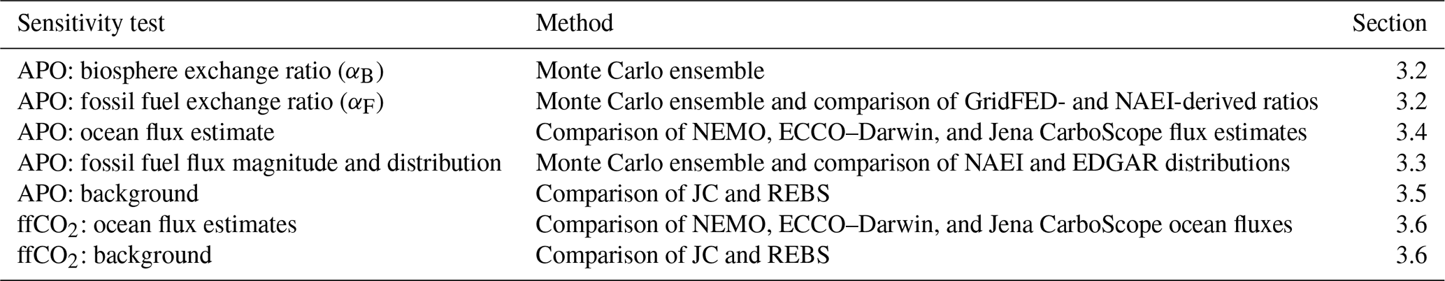
Model simulations of APO are sensitive to uncertainties in several variables of Eq. (5). In this section, we outline how we investigate the sensitivities to the biospheric and anthropogenic exchange ratios (αB and αF), ocean fluxes, fossil fuel CO2 emissions, baseline, and atmospheric model. The sensitivity tests (for APO and ffCO2) are summarized in Table 1.
Table 1Summary of sensitivity tests. The left-hand column indicates the parameter being investigated and whether the sensitivity to APO or ffCO2 is being investigated. The middle column briefly describes the method employed to determine the sensitivity, and the relevant results section is shown to the right.
2.3.1 Sensitivity to the exchange ratios: αB and αF
To investigate our sensitivity to αB and αF in Eq. (5) we employ a Monte Carlo method, randomly generating a value for each from a Gaussian distribution with a standard deviation of 0.04 mol mol−1 (Marshall et al., 2019) and 3 % (Jones et al., 2021) for αB and αF respectively. Doing so, we generate 1000 values for the APO time series.
As αF varies for different fuels, we must take this into account when studying the sensitivity to αF. As described in Sect. 2.2.2, the fossil fuel O2 flux for each sector is calculated using αF based on the proportion of fuels consumed within that sector. We therefore initially investigate the sector-wise sensitivity of the O2 flux to αF for each fossil fuel: coal, oil, and gas. We combine this information to determine the overall sensitivity of the fossil fuel O2 flux and the APO simulation to αF.
2.3.2 Sensitivity to fossil fuel flux magnitude and distribution
We estimate the sensitivity of the modelled APO to changes in the distribution and magnitude of fossil fuel CO2. We investigate the influence of the spatial distribution by comparing APO simulations using the NAEI and EDGAR, which are overall very similar in magnitude but have different distributions (Fig. 2). As discussed in Sect. 2.2, our APO model uses NAEI ffCO2 emission estimates for the UK, which are embedded in those of EDGAR and combined with NAEI fuel usage statistics to calculate ffO2 uptake. We compare these estimates to EDGAR CO2 emissions with GridFED αF.
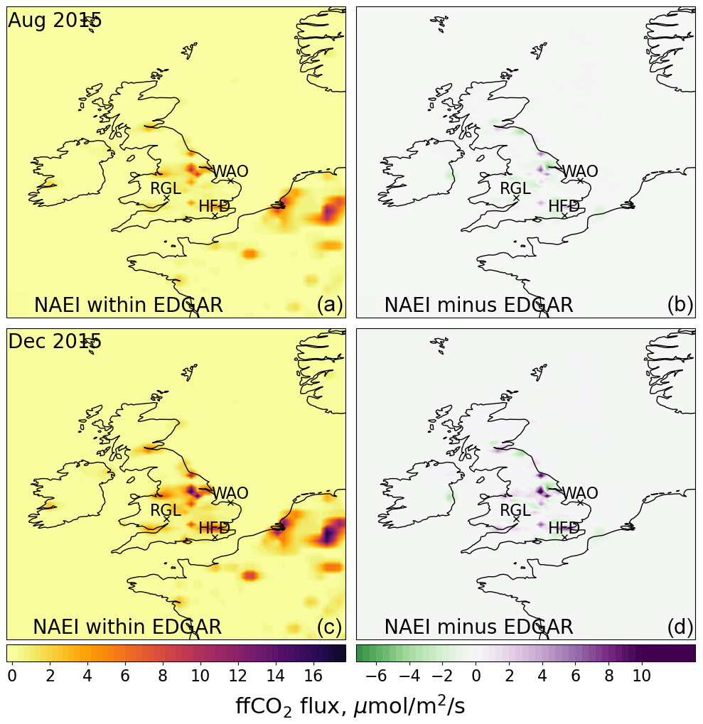
Figure 2The ffCO2 flux estimated by the NAEI, embedded in EDGAR (a, c), and the difference between the NAEI and the EDGAR fields (b, d) for August (a, b) and December 2015 (c, d). By definition, panels (b) and (d) are zero outside of the UK. The crosses show the locations of the sites included in this study: HFD, RGL, and WAO.
We investigate the sensitivity of the APO model to the magnitude of ffCO2 using a Monte Carlo ensemble in which the overall CO2 flux in the entire domain is allowed to vary by ±10 %. This range is considerably larger than the difference between EDGAR and the NAEI, which is approximately 0.7 % but chosen so that the effect on APO can be identified.
2.3.3 Sensitivity to ocean flux
Figure 3 shows the ocean flux fields from the ED and NE models and the JC inversion. This figure is shown for a period (13 August 2015) when the footprint for WAO is predominantly across the ocean. On this date, and in general, there is a much larger flux in coastal regions in the NE ocean model compared to both the ED and JC estimates. Unlike exchange ratios, the sensitivity of simulated APO to ocean fluxes cannot be described by an uncertainty on a single parameter. Therefore, to examine the sensitivity to this term, we produce APO time series using the three different flux estimates such that we can qualitatively compare the effect on APO magnitude and variability and compare the correlation of each model with the observations. We also produce a time series with the ocean component excluded to examine whether the fit to the observations can be improved by assuming a negligible ocean contribution.
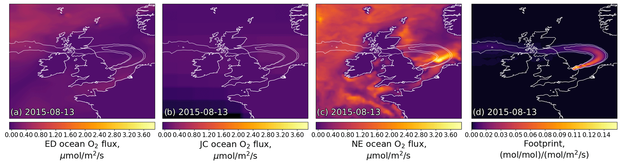
Figure 3The daily mean O2 ocean flux fields from the ED model (a), the JC inversion (b), the NE model (c), and the NAME footprint (d) on 13 August 2015 at WAO, at a time during which the ED and NE ocean fluxes dominate the simulated APO and when there is a large difference between the estimated O2 contribution from the three flux estimates. The flux fields have two example footprints overlaid, corresponding to 0.002 and 0.005 (mol mol−1) (mol m−2 s−1)−1.
2.3.4 Sensitivity to the background estimate
As our APO simulations only account for the influence of fluxes within our regional domain, an estimate must be made of the APO entering the domain. In this section, we describe how different background estimates might influence the comparison between the APO simulation and the observations. The background represents the APO variability that is representative of the well-mixed atmosphere at the UK's latitude, excluding local influences. We compare the modelled Δ(δAPO) (calculated using Eq. 5) with background-subtracted observations at Weybourne throughout 2015. We compare two methods to subtract the background from the observations. First, we estimate a baseline from the APO observations using the “REBS” statistical fitting routine (Robust Extraction of Baseline Signal; Ruckstuhl et al., 2012; Pickers et al., 2022) with a span value of 0.03, equivalent to a smoothing window of approximately 1 week. This smoothing window was thought to be the most appropriate for incorporating wider-scale APO signals from outside Europe into the background term while simultaneously excluding local influences. For our second background subtraction we use the JC background estimate, estimated from boundary conditions propagated to the measurement site using NAME (Sect. 2.2.3). A monthly adjustment is made to the JC background to account for offsets observed in some months, as described in Sect. 2.2.3. This gives us two estimates of observation-derived ffCO2, which we can compare the background subtraction method.
These background estimates are inherently different: for example, the REBS baseline incorporates regional ocean seasonality, whereas the JC estimate represents contributions from outside of the domain. However, comparing both background subtractions gives us an idea of the impact of differences between background estimates, such as their variability.
2.3.5 Sensitivity to the atmospheric model
In this study, we use the NAME atmospheric transport model (Sect. 2.2). Although NAME has been extensively inter-compared to other transport models in several publications (e.g. Brunner et al., 2017; Rigby et al., 2019; Monteil et al., 2020), systematic errors in NAME will influence the comparison with observations. Whilst an extensive model inter-comparison exercise is beyond the scope of this paper, to provide a simple comparison with another widely used modelling system, we compare the NAME fossil fuel CO2 time series to that of CarbonTracker Europe (CTE2022; van der Laan-Luijkx et al., 2017; Friedlingstein et al., 2022). CTE2022 uses the TM5 transport model (Krol et al., 2005) driven by ERA5 meteorology to transport prior fluxes globally, and surface CO2 fluxes are optimized on a weekly time step over the period 2000–2021. The prior fluxes are from the SiB4 Biosphere Model (Haynes et al., 2019), the Global Fire Assimilation System (GFAS) fire emissions (Kaiser et al., 2012), GridFED fossil fuel emissions (Jones et al., 2021), and JC ocean fluxes. CO2 mole fractions based on the optimized CTE2022 at the WAO are used here, with separate tracers available for each of the described flux components.
2.4 Fossil fuel CO2 mole fraction
Previous studies have indicated that we can assume that ocean fluxes do not contribute strongly to the overall APO at a measurement site over short timescales (Pickers, 2016; Pickers et al., 2017; Chevalier and WP4 CHE partners, 2021). Based on this assumption, it has been proposed that we can estimate regional ffCO2 mole fractions from APO, following Pickers (2016):
where δAPObg is a background APO estimate and is the δAPO : ffCO2 ratio which can be estimated from .
To estimate the time-varying ratio in the air intercepted at the measurement site, we use the footprint-weighted fossil fuel exchange ratio:
where t is the time, j is the grid cell, N is the maximum number of grid cells, αFt,j is αF for one grid cell at that time, fpt,j is one grid cell of the hourly footprint at that time, and is the sum of the footprint across all grid cells at that time.
Here we investigate how well we can retrieve ffCO2 mole fraction contributions from our APO simulations, and we also estimate ffCO2 from our observations using Eq. (12). These estimates are directly compared to modelled ffCO2 by multiplying the NAEI-within-EDGAR flux by NAME footprints, as described in Sect. 3.1. Equation (12) requires an estimate of the APO background, δAPObg. When deriving ffCO2 from the model we compare two methods to estimate this term: in one case by fitting a baseline to the APO model using the REBS statistical fitting routine; for comparison we use the adjusted JC background estimate. The baselines for the whole of 2015 are shown in Fig. S9. We then derive ffCO2 from the below-baseline APO, comparing the effect of using a constant value for and of using Eq. (13) to calculate a time-varying exchange ratio.
3.1 Simulated APO at UK measurement sites
Here we show our APO model results for 2015. As examples, one summer month (August) and one winter month (December) are shown. These months were selected based on data availability, statistical goodness-of-fit, and having 2 months that represent sufficiently distinct parts of the APO seasonal cycle. Simulations for all months of 2015 and 2021 are provided in the Supplement (Figs. S3 and S6).
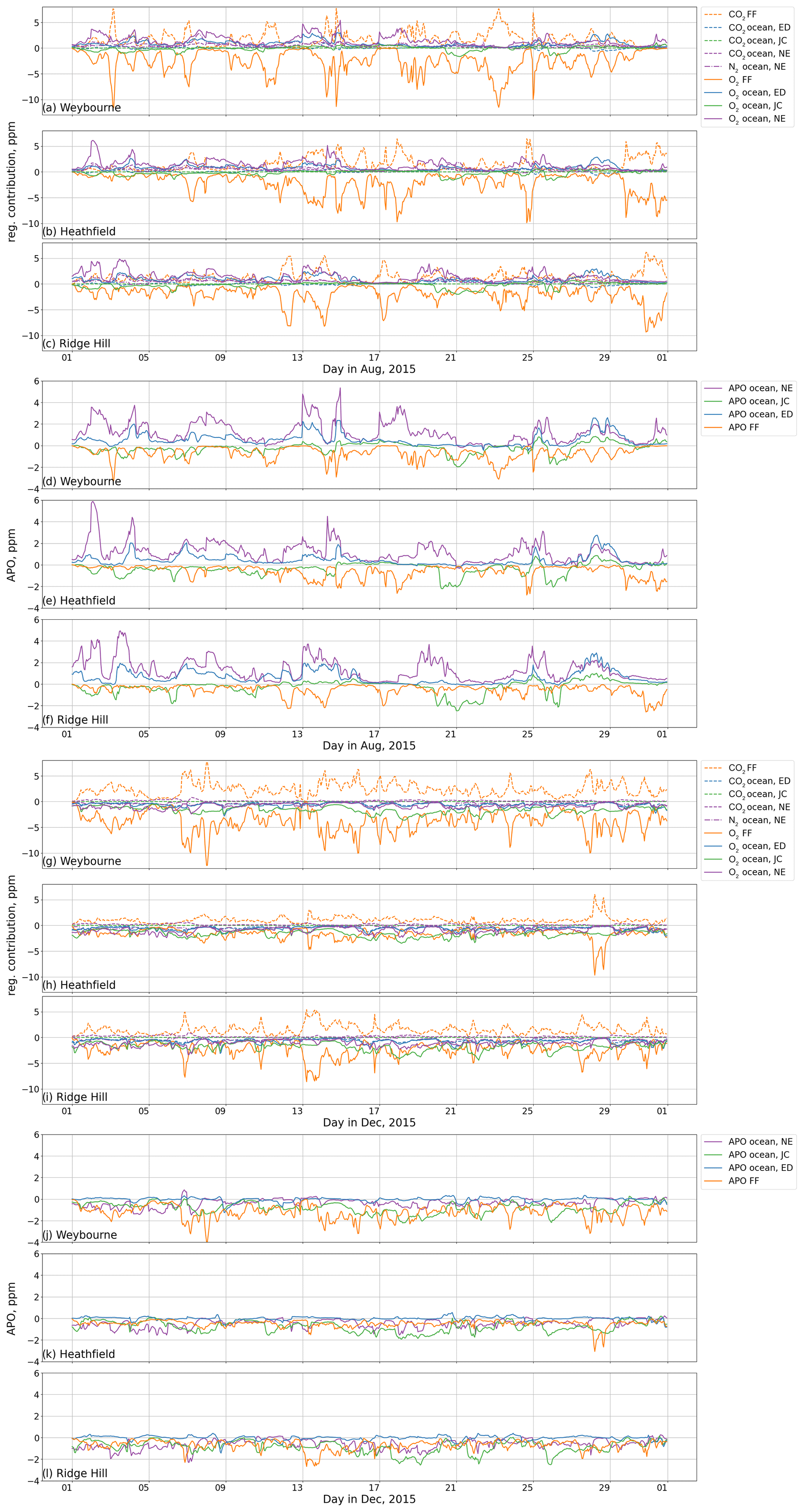
Figure 4The first six panels show the gas-specific sectoral contributions of the ocean and fossil fuel components of APO to the mole fractions of each species at Weybourne, Heathfield, and Ridge Hill (a, b, c) and the APO ocean and fossil fuel contributions to the APO model at the three sites (d, e, f) throughout August 2015. The blue, green, and purple lines show the contributions calculated from the ED, JC, and NE fluxes respectively, and the orange lines show the fossil fuel contributions. Solid lines represent O2 in the top panels and APO in the bottom panels, dashed lines show the CO2, and dash-dotted lines show the N2. The next six panels show the regional contribution of the ocean and fossil fuel components of APO to the mole fraction of each species at Weybourne, Heathfield, and Ridge Hill (g, h, i) and the overall regional ocean and land contribution to the APO model at the three sites (j, k, l) throughout December 2015. The blue, green, and purple lines show the contributions calculated from the ED, JC, and NE fluxes respectively, and the orange lines show the fossil contributions. Solid lines represent O2 in the top panels and APO in the bottom panels, dashed lines show the CO2, and dash-dotted lines show the N2.
The simulated CO2 and O2 mole fractions and APO contribution due to each source and sink are shown in Fig. 4 for August and December 2015 at the three sites. In August, the ocean and fossil fuel mole fraction contributions have similar magnitudes, and there are sustained periods during which the ocean APO component dominates over the fossil fuel component. We find that there are background O2 excursions which are considerably larger than those inferred by Pickers et al. (2017). However, there is a large disagreement between the three models of ocean APO contribution, and the difference between them is frequently of a similar magnitude to that of their contribution. Whereas over the summer the ED and JC models suggest net oxygen release from the ocean, over the winter we see overall uptake due to the differences in temperature and solubility, as well as the balance of respiration and productivity. In December, the magnitude of the fossil CO2 and O2 mole fractions is larger than that of the ocean, although there are still large differences between the ocean models. However, when converted to the fossil fuel and ocean components of APO, the magnitudes are similar for Weybourne, and for much of December the fossil fuel component is small compared to the ocean at Heathfield and Ridge Hill, despite these sites being further inland than WAO. For all three sites, variation between the ocean models is comparable to the magnitude of their flux, and there are large periods of December during which the ocean is dominant as an O2 sink. This is in contrast to the findings of Chevalier and WP4 CHE partners (2021), who found that the fossil fuel APO contribution was dominant at all sites, including Weybourne and Heathfield. That study used a combination of fluxes from NEMO–PlankTOM5 and the atmospheric transport model STILT (Lin et al., 2003). However, Chevalier and WP4 CHE partners (2021) do not provide details on the magnitude of variability in these flux estimates.
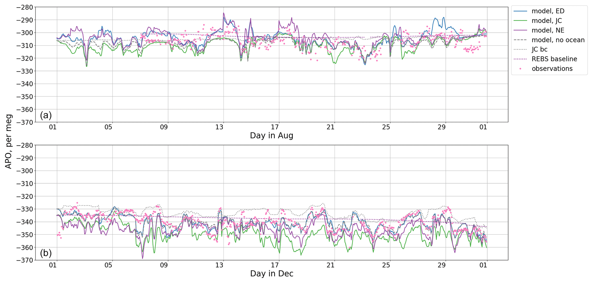
Figure 5The modelled and observed APO at Weybourne throughout August (a) and December (b) 2015, where we model APO using three different ocean flux estimates from the global ED ocean model (blue), the global JC inversion (green), and the regional NE ocean model (purple). We also show the APO model with no ocean contribution (dashed grey line). The dotted grey line shows the baseline derived from JC boundary conditions, which has been adjusted as described in Sect. 2.2.3. The magenta dots show the observations, and the dotted purple line shows the baseline fit to the observations using the statistical fitting routine REBS.
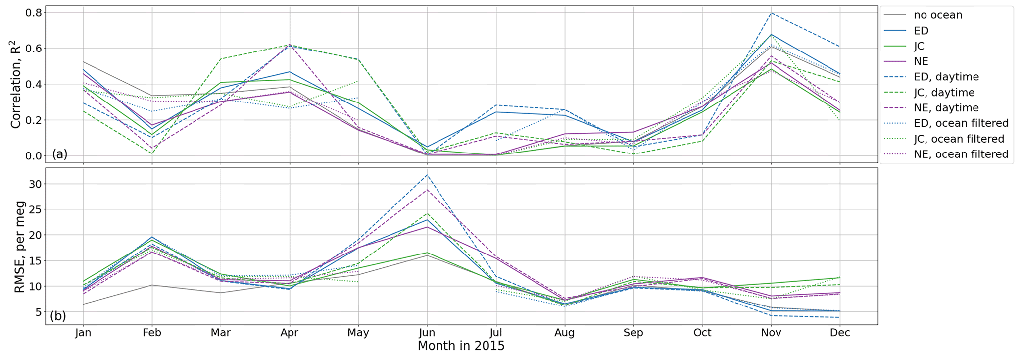
Figure 6R2 (a) and the root-mean-square error (RMSE) (b) of the modelled APO compared to the observations at Weybourne in 2015. The blue, green, purple, and grey lines show the results from the models derived using the NAME simulations and either ED, JC, NE, or no ocean fluxes respectively. The solid, dashed, and dotted lines respectively show the correlations when we do not apply any filter, when we filter for just daytime hours, and for times when the footprint has at least 40 % sensitivity to the land.
Combining the APO components using Eq. (5) gives a modelled APO for Weybourne, as shown in Fig. 5 (for all three sites in 2015 see Fig. S3, and for Weybourne and Heathfield in 2021 see Fig. S6). We find that although the magnitude of the variability is similar, there are substantial differences between the simulations and the observations. Figure 6 shows the R2 and root-mean-square error (RMSE), comparing each set of APO simulations and the observations at Weybourne for each month throughout 2015. The mean of all the APO simulations for December gives a closer fit to the observations at Weybourne than the mean of all the APO simulations in August (average R2 of 0.34 vs. 0.10 and average RMSE of 7.1 vs. 8.4 per meg for December and August respectively). We see a clear seasonal trend, that the correlation is lowest throughout the summer and winter and increased during the spring and autumn. This is shown in Fig. S4, where there is larger scatter over the summer months. As discussed above and shown in Fig. 5, we also find that the model is more sensitive to the ocean flux over the summer, when the difference between the three APO simulations using different ocean fluxes is substantially larger (a monthly average of 7.0 per meg difference between the smallest and largest estimate in August, compared to 3.8 per meg in December). However, although our model agreement may be affected by ocean fluxes, we do not see a substantially better or worse fit when we exclude the ocean fluxes entirely, as shown in Fig. 6. The R2 and RMSE for the CO2 and O2 models are shown in Fig. S5, where we generally see higher correlations with the data for the CO2 and O2 simulations (R2 generally above 0.4) than we do for APO. We also find that our 2021 model, shown in Fig. S6, does not display such large variability. In that simulation, we use ocean climatologies, finding that localized ocean emission or uptake events are smoothed as they are averaged across a number of years.
Next we try filtering our model in two ways to see the effects on the correlation with the observations. First, we study only daytime hours (between 11:00 and 15:00 LT) as the planetary boundary layer is generally more well-mixed during the day than at night, and so it is often assumed that the model–data mismatch will be smaller. Separately, we filter for times at which the footprint has at least 40 % sensitivity to the land, to investigate the effects of reducing the influence of ocean-dominated time steps. With both tests we see a small improvement in the correlation in some months. Overall, the difference in the simulations without filtering is small (Fig. 6). We further discuss the sensitivity to the ocean fluxes in Sect. 3.4.
3.2 Sensitivity to exchange ratios
The 3σ sensitivity of APO to αB and αF is shown in Fig. 7 (3σ is shown so that changes can be seen). In general, the model is more sensitive to αF than αB (average 1σ interval of 0.27 and 0.41 per meg for αB in August and December 2015 respectively, compared to 0.30 and 0.52 per meg for αF). For both variables, the influence on APO of a 1σ change is generally small compared to the difference between the observations and the model that we see in Fig. 5. We see larger sensitivity to both values of α when the mole fraction is dominated by fossil fuel fluxes. Chevalier and WP4 CHE partners (2021) also identified an influence on the simulated APO due to potential misspecification of αB.
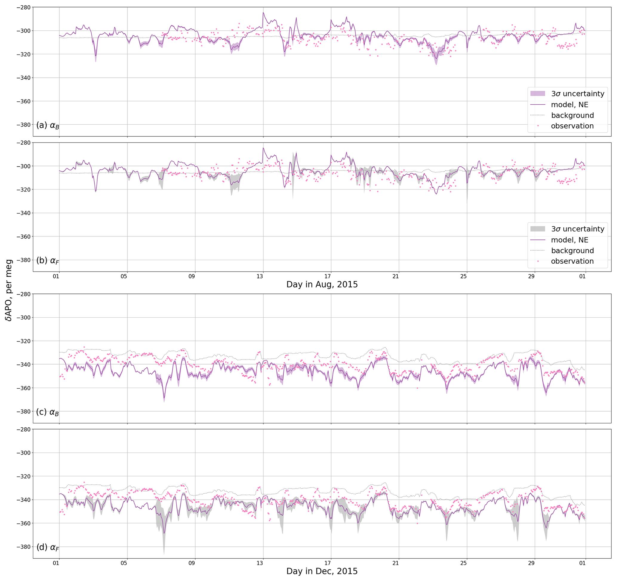
Figure 7APO at Weybourne during August (a, b) and December (c, d) 2015 and the sensitivity to αB and αF. The magenta points are the observations, the purple line is the model using NE ocean O2 fluxes, and the shaded region is the 3σ range derived from a Monte Carlo ensemble in which αB (purple, panels a and c) and αf (grey, panels b and d) are sampled.
3.3 Sensitivity to fossil fuel CO2 flux
Figure 8 shows APO at Weybourne, with fossil fuel sources modelled using a combination of fluxes and exchange ratios as follows: NAEI (within EDGAR) with NAEI exchange ratios (labelled “NAEI”), EDGAR with GridFED exchange ratios (“EDGAR–GridFED”), and NAEI with GridFED exchange ratios (“NAEI–GridFED”). We find that although there are variations in the magnitude at some time steps, the variability of the EDGAR and NAEI fossil fuel APO models is very similar. For the most part, the two models agree, with high R2 in both August and December 2015, as shown in Table 2. This suggests that the choice of inventory does not have a significant impact on the simulations compared to the other components that we investigated. Additionally, in agreement with the findings of Sect. 3.2, the model does not seem highly sensitive to αF: the application of different fossil fuel exchange ratios to estimate the O2 uptake does not cause a strong disagreement between the two fossil fuel O2 models in Fig. 8, which have a high R2.
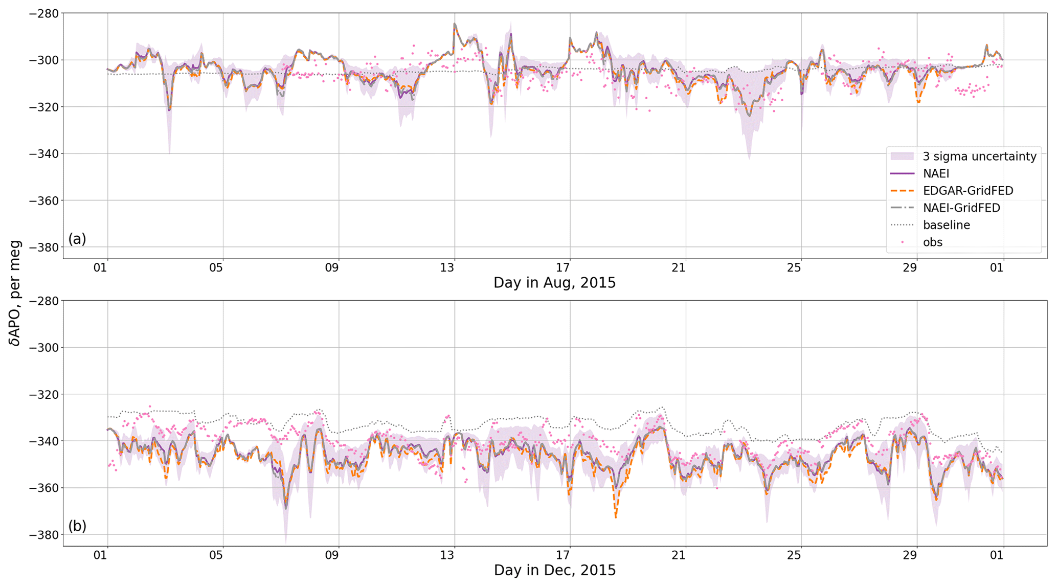
Figure 8The APO model at Weybourne in August (a) and December (b) 2015 using NAME footprints and O2 fluxes from the NE ocean model, compared to the model using NAEI fluxes and exchange ratios (purple), to that using NAEI fluxes and GridFED exchange ratios (grey), and to that using EDGAR fluxes and GridFED exchange ratios (orange). The observations are shown in magenta; the shaded regions represent the 3σ uncertainty in the model, assuming a 10 % 1σ uncertainty on the fossil fuel component; and the dotted grey line is the background derived from JC boundary conditions.
Table 2R2 for August and December 2015, comparing the modelled APO using NAEI CO2 fluxes and exchange ratios, EDGAR CO2 fluxes with GridFED exchange ratios, and NAEI CO2 fluxes with GridFED exchange ratios. For these APO models we use the NE O2 ocean flux estimates.
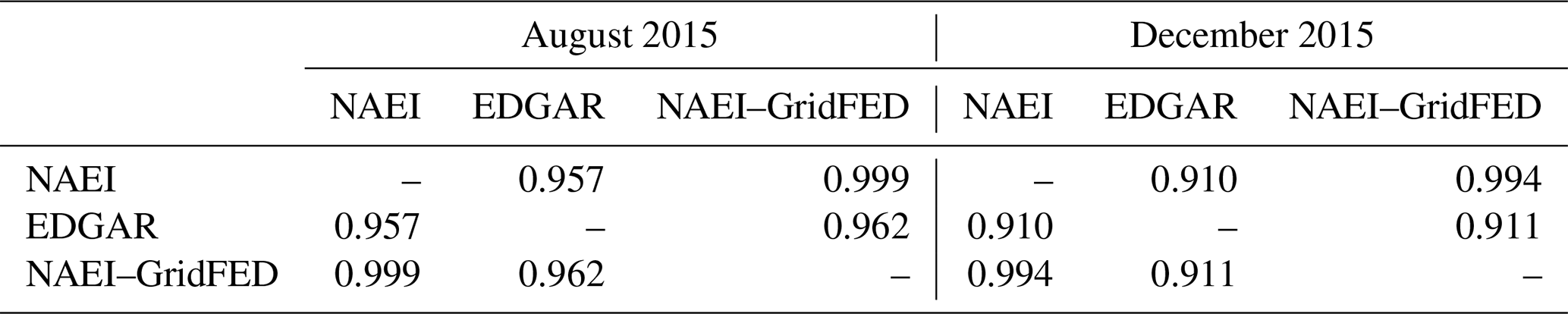
Figure 8 shows the modelled APO time series and the associated 3σ range when sampling the magnitude of fossil fuel emissions with a 10 % standard deviation. The sensitivity is highest when air comes from populated areas. However, these periods of high sensitivity do not necessarily coincide with times when the discrepancy between the model and observations is highest, suggesting that errors in fossil fuel fluxes alone could not explain some of the differences between the model and the observations.
3.4 Sensitivity to ocean flux
When comparing APO models and observations in Fig. 6 (and Figs. S3 and S4), we find the biggest disagreement during the summer. At this time of year there is increased ocean productivity compared to over the winter; thus the variations between the models are larger and the APO models vary more widely. Conversely, the highest correlation between all models and the observations is seen in October (see Fig. S7), when the ocean acts as a small O2 sink and the O2 ocean flux is smallest of any month. We see in Figs. 4, 5, and S3 that the models using the ED and NE fluxes exhibit large events of O2 release throughout the summer, which are more exaggerated in NE. At some of these times we see large differences between the ED and NE models compared to the model with no ocean component, as the ocean models indicate large APO excursions. Between April and June especially, there are excursions in the NE APO model which have a much larger magnitude (up to ∼ 85 per meg) than any in the observations. On the other hand, JC shows much smaller O2 fluxes with generally smoother variations and even suggests some negative APO contribution from the ocean during the summer. At some points during the summer we therefore see increased variability with NE compared to the other models. This difference may be due to the handling of coastal fluxes and the influence of rivers, which are more finely resolved in NE with its higher spatial resolution (∼ 7 km vs. ∼ 18 km), with explicit nutrient input from rivers, and by a more detailed representation of physiological processes of phytoplankton (e.g. variable stoichiometry). Another factor that could contribute to differences between estimates of O2 air–sea fluxes between ocean models is the differences in the wind products used to drive the air–sea exchange and their spatial and temporal resolution.
Based on our investigation we cannot determine which, if any, of the ocean flux estimates represent the APO contribution at sites in the UK. Furthermore, we do not see a substantial difference in correlation between the observations and either the simulations that include ocean fluxes or those that do not. Chevalier and WP4 CHE partners (2021) also noted an ocean influence in their simulations using different transport models to those used here. Our result requires further investigation, since the magnitude of some of the short-term ocean variability during the summer in NE and ED simulations is inconsistent with what is seen in the observations at WAO. Furthermore, the extent to which these findings are due to the coastal location of WAO needs to be determined, since some shipboard measurements do not show a large sensitivity to ocean fluxes (Pickers, 2016). Rödenbeck et al. (2023) suggest that a dense continental network of stations measuring APO could minimize the potential influence of oceanic fluxes, meaning that robust estimates of fossil fuel CO2 fluxes could be made by using observed APO gradients within a continent.
3.5 Sensitivity to the background estimate
Figure 9 shows the modelled regional Δ(δAPO) and the background-subtracted observations. We compare the background subtraction from the statistical (REBS) filter with the adjusted model-estimated baseline from the JC global fields. For most of the time series, the two baseline estimates lead to similar regional signals. In December there is more of a difference between the two signals, where at some regions the REBS subtracts a smaller background and leaves positive APO excursions. We expect that this difference arises because there is more variability within the JC background estimate. We see in Fig. S2 that this variability is increased in the winter compared to in the summer. We see in Fig. 10 that the correlation between the background-subtracted observations and the models is similar for both methods of background subtraction. Neither choice leads to a substantial difference in model–data mismatch.
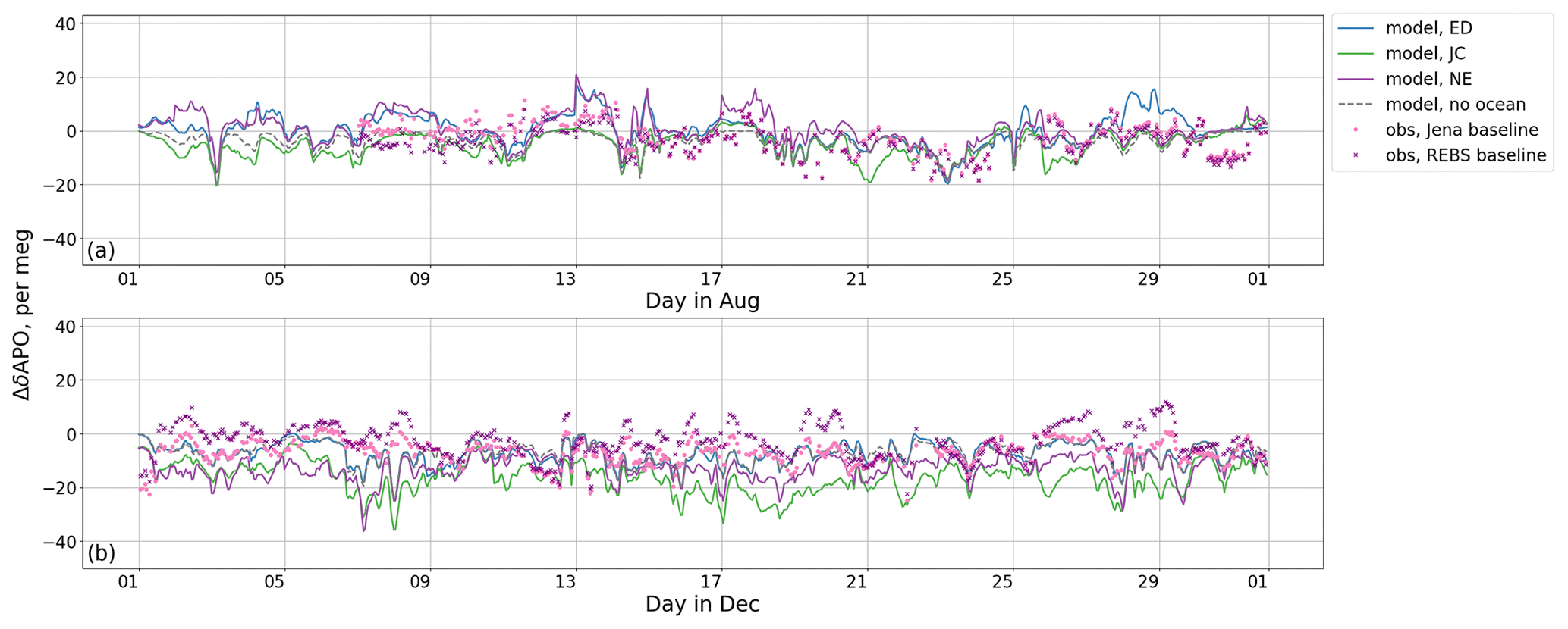
Figure 9The modelled regional APO contribution and the background-subtracted APO observations at Weybourne throughout August (a) and December (b) 2015, where we model APO using three different ocean flux estimates from the global ED ocean model (blue), the global JC inversion (green), and the regional NE ocean model (purple). We also show the APO model with no ocean contribution (grey line). We show two versions of background subtraction using a statistical routine (REBS, purple crosses) and using the JC background (pink points).
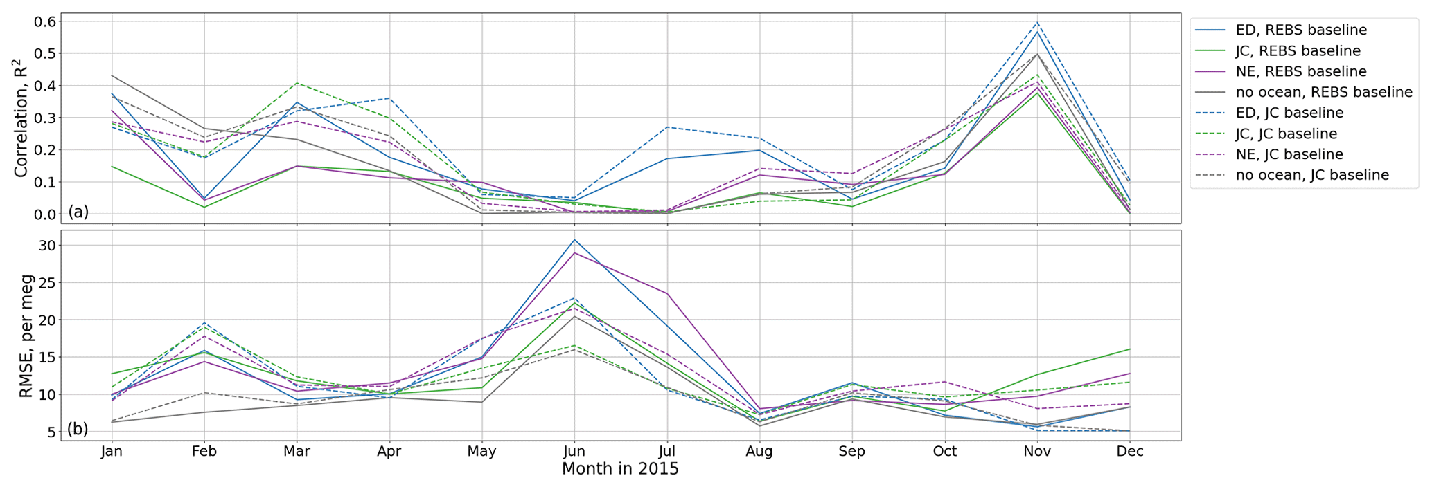
Figure 10The square of the Pearson correlation coefficient (R2) (a) and the RMSE (b) of the modelled regional contribution of APO compared to the background-subtracted observations at Weybourne in 2015. The blue, green, purple, and grey lines show the results from the models derived using the NAME simulations and either ED, JC, NE, or no ocean fluxes respectively. The solid and dashed lines respectively show the results when we subtract the REBS statistical background from the observations and when we subtract the JC-derived background.
3.6 Estimation of fossil fuel CO2
We test how well we can retrieve the regional contribution of ffCO2 from our modelled APO, using the method described in Sect. 2.4. Figures 11 and S10 show the comparison between ffCO2 derived from our modelled APO and the direct simulation of ffCO2 using NAME (i.e. ffCO2 fluxes multiplied by NAME footprints). The comparison for all months throughout 2015 and the correlations are shown in Fig. S10. Comparisons are shown when three different ocean flux estimates are used or when two different methods are used for subtracting the baseline. Differences between the APO-derived ffCO2 and the direct ffCO2 simulation will be due to the influence of ocean fluxes on the APO simulation (which is assumed negligible in Eq. 12) and misspecification of the background. All other factors, including atmospheric transport, are consistent between the two sets of simulations. Therefore, the APO-derived ffCO2 using the adjusted JC background exactly matches the direct ffCO2 simulation if ocean fluxes are zero.
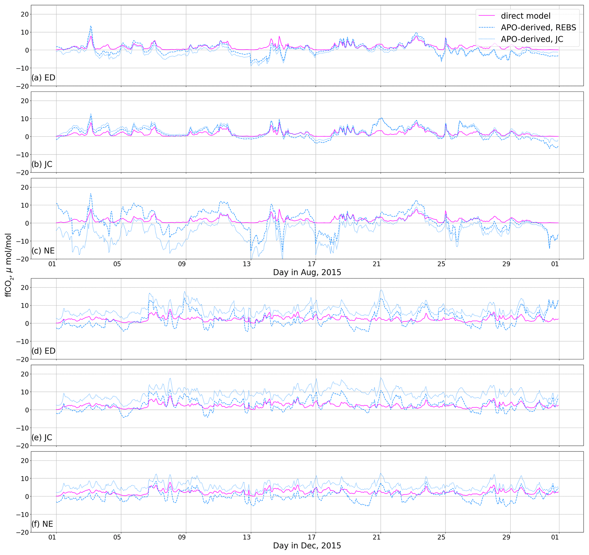
Figure 11The modelled ffCO2 for August (a, b, c) and December (d, e, f) 2015 derived from the APO model for Weybourne using the results from three different ocean flux fields (blue): ED (a, d), JC (b, e), and NE (c, f). We compare to the model calculated directly from the NAEI-within-EDGAR fluxes and NAME footprints (pink). The direct model is equivalent to the ffCO2 in the top panels of Fig. 4, and the APO models are shown in Fig. 5.
Firstly, we will consider the APO-derived ffCO2 using the adjusted JC backgrounds. Throughout the summer, when there are large O2 release events in the modelled ocean fluxes, the APO simulation using NE generally underestimates ffCO2, even indicating negative mole fractions for large parts of the month. The ED and JC APO simulations show closer overall agreement with ffCO2 in August, although some discrepancy remains for all three. All three models overestimate the ffCO2 for the majority of the winter compared to the direct ffCO2 simulation. In this case the background APO, estimated as described in Sect. 2.4, is underestimated for large parts of the month, which may be due to modelled oceanic uptake of oxygen around the UK throughout the winter. Chevalier and WP4 CHE partners (2021) found high correlations between their APO-derived ffCO2 and direct STILT model. The period over which this correlation was found is unclear from their work. We find that our correlation is greatly improved when averaging over larger time periods due to the seasonality in APO.
For the simulations where the REBS baseline has been fitted to the APO simulations and then subtracted, the derived ffCO2 from ED and NE is higher during the summer and lower during the winter than when the adjusted JC background is used. For the model that used JC ocean fluxes, which are considerably smaller than either ED or NE, there is a much smaller difference between the two estimates. The large difference between the simulations using these two baseline estimates likely stems from the influence of ocean fluxes. The REBS fit incorporates seasonal oceanic trends and removes long-timescale oceanic fluxes from the model. However, it is also susceptible to fitting to large APO excursions in the model which occur due to modelled short-term variability from the ocean. This is clear throughout June in Fig. S9. On the other hand, as JC is independent of the model, it does not encapsulate any regional ocean influence, and any ocean contribution is treated as ffCO2.
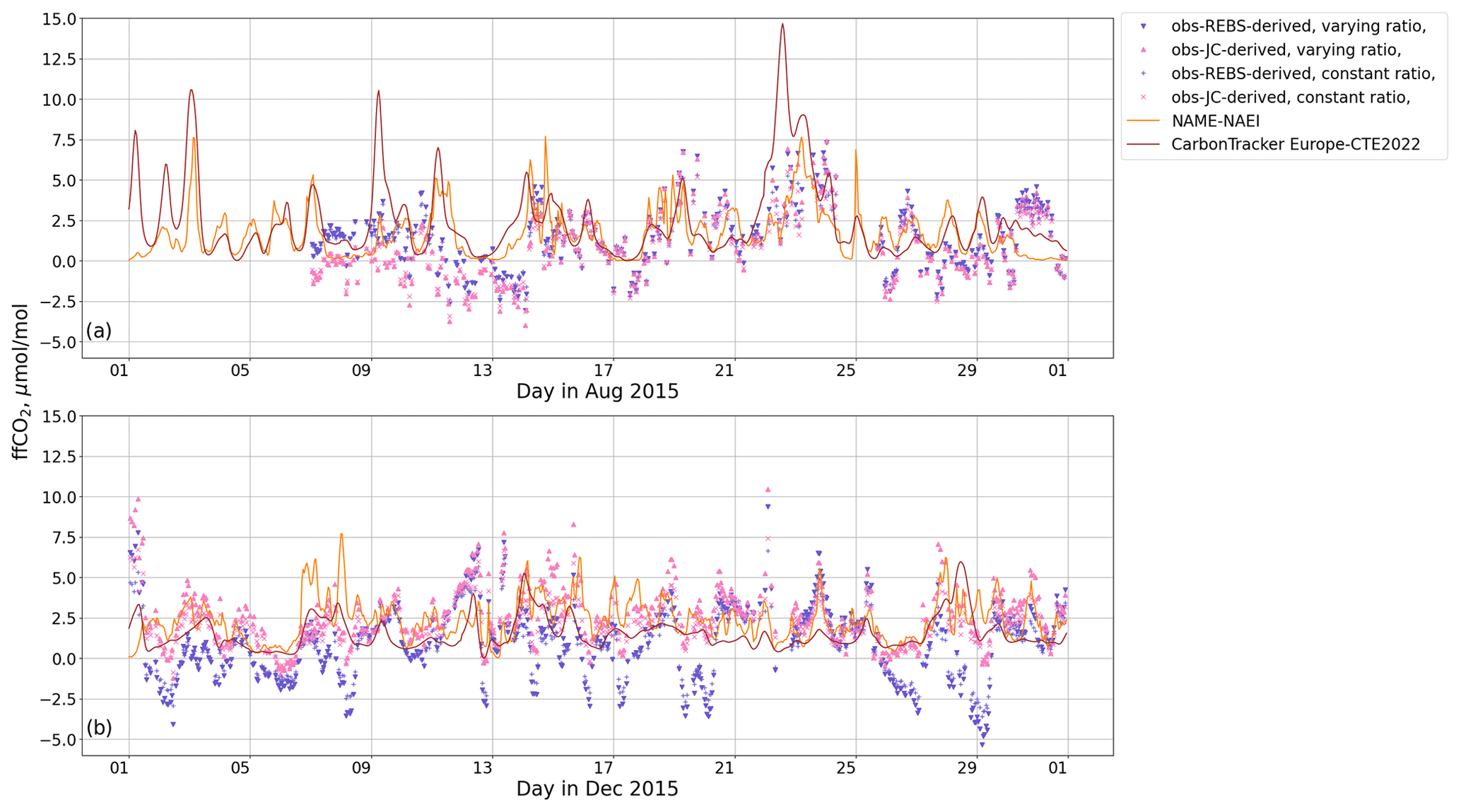
Figure 12The regional contribution of ffCO2 to the atmospheric abundance at Weybourne for August (a) and December (b) 2015. The pink triangles and crosses show the ffCO2 model derived from the APO observations with the JC background subtracted using a time-varying and a constant exchange ratio respectively. The purple triangles and pluses show the same but with the REBS baseline subtracted, the orange line shows the model calculated directly from the NAEI-within-EDGAR fluxes and NAME footprints (equivalent to that in the top panels of Fig. 4), and the brown line shows the model derived from CarbonTracker Europe (CTE2022).
In Sect. 2.4 we make the assumption that the ocean component of the APO measurements is negligible when deriving ffCO2. This is based on previous studies of short-term ocean-related APO variability, which in turn are based on observations. However, these models all indicate a persistent ocean contribution at all sites, which biases our calculation of ffCO2 from the APO simulations. As shown in Sect. 3.1, there is a large variation in O2 flux estimates between ocean models. We cannot conclude which model, if any, gives a more accurate representation of the ocean O2 flux. Furthermore, CO2 and O2 ocean fluxes are decoupled; therefore the exchange ratio varies as the footprint intercepts different parts of the ocean. Based on our analysis using these three ocean flux estimates, a correction for oceanic fluxes would be subject to substantial uncertainty.
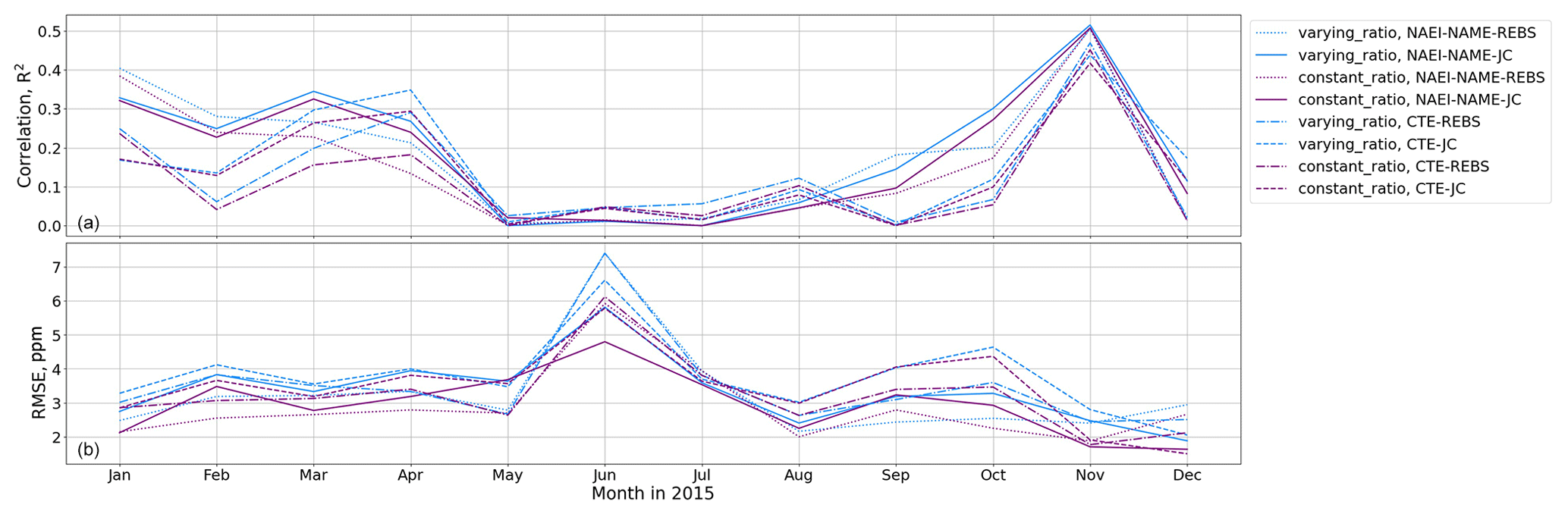
Figure 13The R2 (a) and the root-mean-square error (RMSE) (b) of the model-derived and observation-derived ffCO2 at Weybourne in 2015. The blue and purple lines show the correlation when using a time-varying and a constant APO : ffCO2 ratio respectively, the solid lines show the correlation between the NAME–NAEI model and the JC background-subtracted observations, and the dotted lines show the same but with the REBS-background-subtracted observations. The dashed lines show the correlation between the CTE model and the JC background-subtracted observations, and the dash-dotted lines show the same but with the REBS background-subtracted observations.
Next we apply the same method to estimate ffCO2 from the observed APO at Weybourne (Pickers et al., 2022) as described in Sect. 2.4. Figure 12 shows observation-derived ffCO2 compared to the direct ffCO2 simulations. Here, we have used the NAME simulation with NAEI and EDGAR fluxes and also the outputs of the CTE system. The correlations (R2) between the observation-derived ffCO2 and the ffCO2 model are shown in Fig. 13. As we found in Sect. 2.2, we see low correlations over the summer, with stronger agreement in March, April, and November. There is not a large difference in the correlation for the JC and REBS background subtractions. This is contrary to our findings shown in Fig. 11, where we see that there are sometimes large differences in ffCO2 estimates for different methods of background subtraction. This is due to the large ocean contribution, which was assumed to be encapsulated in the background estimate. Throughout December we find when using the REBS background-subtracted observations that we frequently estimate negative ffCO2 contributions. These are not as apparent when subtracting the JC background. This could be a result of increased variability in the JC background estimate. Based on the synthetic data results presented in the previous paragraphs, discrepancies may be because of the influence of non-negligible ocean flux contributions or errors in assigning baseline values. At certain times we see an ∼ 5–8 µmol mol−1 difference between the direct model and the observation-derived ffCO2 using the REBS background subtraction. This translates to an ocean contribution of ∼ 10–20 per meg. This would be a large contribution, although the majority of the differences between the estimates are much smaller than this.
We also test the conversion of the APO observations to ffCO2 using a constant APO : ffCO2 ratio, assuming , as shown by the blue points in Fig. 12. Throughout the year, the correlation between this estimate of ffCO2 and the direct model are slightly lower than when using a time-varying APO : ffCO2 ratio; thus we find that using a time-varying APO : ffCO2 ratio gives a slightly closer fit to the direct ffCO2 simulation.
Here, we have found model–data discrepancies for APO that are relatively large compared to model–data discrepancies for O2 and CO2 at Weybourne in the UK. This work has used model simulations to understand the factors that could most strongly influence these differences, which can hopefully now inform further observation-based studies. In particular, a better understanding of oceanic CO2 and O2 fluxes in coastal regions was the most important factor in our simulations. If a substantial oceanic influence is confirmed, continental sites far from ocean influence may currently be more viable for fossil fuel CO2 estimation using APO and/or substantially more dense APO measurement networks will be required to account for these fluxes (e.g. Rödenbeck et al., 2023). In future, the development of alternative tracers that are sensitive to ocean fluxes and insensitive to terrestrial sources may help us better understand their relative influences. We also found that the choice of baseline affects our APO model and derived ffCO2, although errors in assigning regional baselines may also be due in part to the influence of non-terrestrial fluxes.
Alongside APO, other tracers such as radiocarbon and CO can give extra insight into regional ffCO2 emissions. Several studies have shown that radiocarbon is a promising tool for this (e.g. Levin et al., 2003; Graven et al., 2009; Zazzeri et al., 2023). However, unlike APO, most radiocarbon programmes rely on flask measurements which are not continuous and require time-consuming analysis. This makes radiocarbon a comparatively expensive method which cannot presently provide such insight into high-frequency variability. Radiocarbon measurements are also susceptible to contamination of 14C emissions from nuclear power plants. The impact of nuclear power plant 14C emissions can be accounted for by using emissions data and information about venting times from individual nuclear power plants. However, these data are challenging to obtain. Although CO measurements are much cheaper than radiocarbon and can be made continuously (e.g. Andrews et al., 2014; Levin and Karstens, 2007; Levin et al., 2020), the conversion from CO to ffCO2 is uncertain.
Given the challenges of each, further work is required to improve each of these tracers for ffCO2 emissions evaluation. Here, we have identified key areas of focus which may improve the use of APO for this purpose in the future.
We have simulated the tracer APO throughout the years 2015 and 2021 at three sites in the UK: Weybourne, Heathfield, and Ridge Hill. Generally, the correlation with the observations is smaller for APO than for simulations of CO2 and O2. We find that modelled ocean signals sometimes dominate the APO model and that correlations tend to be higher for APO during the spring and autumn when ocean fluxes are smallest.
We have presented a sensitivity analysis of the factors that most strongly influence modelled atmospheric APO. Our simulations suggest that uncertainties in ocean fluxes contribute substantially to modelled APO and APO-derived ffCO2 at measurement sites in the UK. Our analysis cannot determine which ocean model (or, indeed, zero ocean flux) or baseline estimation method leads to the closest agreement with the observations. A robust estimate of ffCO2 is likely to depend strongly on these factors being well-known or being proven to have little influence using observation-based methods. We do not find evidence from our three UK stations that the substantial (yet uncertain) influence of oceanic fluxes on simulated APO is reduced further inland, but since the UK is surrounded by ocean, simulated APO at continental European locations may be less strongly affected. More robust ffCO2 estimates may be possible if a sufficiently dense network of sites were available, which could account for fossil fuel influences jointly with those of any oceanic sources. In comparison to the ocean fluxes and baseline, the sensitivity of APO to uncertainties in fossil fuel and terrestrial biosphere exchange ratios was relatively small. Our analysis shows that further work should focus on improving ocean O2 and CO2 flux estimates which could improve the agreement between modelled and observation APO-derived estimates of UK ffCO2.
The code for the analysis presented is available at https://doi.org/10.5281/zenodo.7688294 (Chawner, 2023). We also use code developed by the ACRG at the University of Bristol, which is available at https://doi.org/10.5281/zenodo.6834888 (Rigby et al., 2022).
The datasets generated and analysed during this study are available at https://doi.org/10.5281/zenodo.7681834 (Chawner et al., 2023). The observational datasets are available on CEDA:
-
Heathfield CO2 and O2. https://catalogue.ceda.ac.uk/uuid/bfc2483537a744dca8e3239278b6e522 (Adcock and Pickers, 2022).
-
Weybourne CO2. https://catalogue.ceda.ac.uk/uuid/87fc265aab6b4aeb961e62da2cd6ca91 (Forster, 2022a).
-
Weybourne O2. https://catalogue.ceda.ac.uk/uuid/b3f9714c956f428a840211e0184e23eb (Forster, 2022b).
The supplement related to this article is available online at: https://doi.org/10.5194/acp-24-4231-2024-supplement.
HC carried out the atmospheric modelling and data analysis with contributions from PAP, YA, AM, CR, GL, PL, and ITL. Measurements were made by KEA and PAP, with support from TA, CD, GLF, and CR. HC wrote the paper, with contributions from MR, PAP, ES, YA, ITL, HG, AG, and all co-authors.
The contact author has declared that none of the authors has any competing interests.
Publisher's note: Copernicus Publications remains neutral with regard to jurisdictional claims made in the text, published maps, institutional affiliations, or any other geographical representation in this paper. While Copernicus Publications makes every effort to include appropriate place names, the final responsibility lies with the authors.
Hannah Chawner, Eric Saboya, Matthew Rigby, and Anita Ganesan were supported by a Natural Environment Research Council (NERC) grant to the University of Bristol as part of the Detection and Attribution of Regional greenhouse gas Emissions (DARE-UK) project, NE/S004211/1. Ingrid T. Luijkx received funding from the Dutch Research Council (VI.Vidi.213.143 and 2023/ENW/01426235). We thank Phillip Wilson and Thomas Barningham for assisting with maintaining the WAO O2 and CO2 measurement system during 2015.
Atmospheric O2 and CO2 measurements at the WAO in 2015 and 2021 were funded by the U.K. Natural Environment Research Council (NERC) grants NE/I013342/1, NE/S004521/1, and NE/R011532/1. The WAO atmospheric O2 and CO2 measurements have also been supported by the UK National Centre for Atmospheric Science (NCAS) from 1 December 2013 onwards. Penelope A. Pickers, Karina E. Adcock, and Grant L. Forster received funding from the NERC project, DARE-UK (NE/S004211/1), and Penelope A. Pickers and Karina E. Adcock have received funding from the Horizon Europe project, PARIS (101081430).
Yuri Artioli and Gennadi Lessin acknowledge DARE-UK (NE/S004947/1) and the NERC National Capability programme, Climate Linked Atlantic Sector Science (NERC grant no. NE/R015953/1).
This research has been supported by the Natural Environment Research Council (grant nos. NE/S004211/1, NE/I013342/1, NE/S004521/1, and NE/R011532/1).
This paper was edited by Qiang Zhang and reviewed by four anonymous referees.
Adcock, K. and Pickers, P.: Continuous measurements of atmospheric carbon dioxide (CO2) and oxygen (O2) at Heathfield Tower 2021–2022, NERC EDS Centre for Environmental Data Analysis [data set], https://catalogue.ceda.ac.uk/uuid/bfc2483537a744dca8e3239278b6e522 (last access: 13 March 2024 ), 2022. a
Adcock, K. E., Pickers, P. A., Manning, A. C., Forster, G. L., Fleming, L. S., Barningham, T., Wilson, P. A., Kozlova, E. A., Hewitt, M., Etchells, A. J., and Macdonald, A. J.: 12 years of continuous atmospheric O2, CO2 and APO data from Weybourne Atmospheric Observatory in the United Kingdom, Earth Syst. Sci. Data, 15, 5183–5206, https://doi.org/10.5194/essd-15-5183-2023, 2023. a, b, c
Andrews, A. E., Kofler, J. D., Trudeau, M. E., Williams, J. C., Neff, D. H., Masarie, K. A., Chao, D. Y., Kitzis, D. R., Novelli, P. C., Zhao, C. L., Dlugokencky, E. J., Lang, P. M., Crotwell, M. J., Fischer, M. L., Parker, M. J., Lee, J. T., Baumann, D. D., Desai, A. R., Stanier, C. O., De Wekker, S. F. J., Wolfe, D. E., Munger, J. W., and Tans, P. P.: CO2, CO, and CH4 measurements from tall towers in the NOAA Earth System Research Laboratory's Global Greenhouse Gas Reference Network: instrumentation, uncertainty analysis, and recommendations for future high-accuracy greenhouse gas monitoring efforts, Atmos. Meas. Tech., 7, 647–687, https://doi.org/10.5194/amt-7-647-2014, 2014. a, b
Barningham, T.: Detection and attribution of Carbon Cycle Processes from Atmospheric O2 and CO2 measurements at Halley Research Station, Antarctica and Weybourne Atmospheric Observatory, UK, PhD thesis, University of East Anglia, https://ueaeprints.uea.ac.uk/id/eprint/68343 (last access: 13 March 2024), 2018. a
Battle, M., Fletcher, S. M., Bender, M., Keeling, R. F., Manning, A. C., Gruber, N., Tans, P. P., Hendricks, M. B., Ho, D. T., Simonds, C., Mika, R., and Paplawsky, B.: Atmospheric potential oxygen: New observations and their implications for some atmospheric and oceanic models, Global Biogeochem. Cy., 20, GB1010, https://doi.org/10.1029/2005GB002534, 2006. a
Blaine, T. W., Keeling, R. F., and Paplawsky, W. J.: An improved inlet for precisely measuring the atmospheric Ar N2 ratio, Atmos. Chem. Phys., 6, 1181–1184, https://doi.org/10.5194/acp-6-1181-2006, 2006. a, b
Bozhinova, D., Palstra, S. W. L., van der Molen, M. K., Krol, M. C., Meijer, H. A. J., and Peters, W.: Three Years of Δ14CO2 Observations from Maize Leaves in the Netherlands and Western Europe, Radiocarbon, 58, 459–478, https://doi.org/10.1017/RDC.2016.20, 2016. a
Brix, H., Menemenlis, D., Hill, C., Dutkiewicz, S., Jahn, O., Wang, D., Bowman, K., and Zhang, H.: Using Green's Functions to initialize and adjust a global, eddying ocean biogeochemistry general circulation model, Ocean Model., 95, 1–14, https://doi.org/10.1016/j.ocemod.2015.07.008, 2015. a
Brunner, D., Arnold, T., Henne, S., Manning, A., Thompson, R. L., Maione, M., O'Doherty, S., and Reimann, S.: Comparison of four inverse modelling systems applied to the estimation of HFC-125, HFC-134a, and SF6 emissions over Europe, Atmos. Chem. Phys., 17, 10651–10674, https://doi.org/10.5194/acp-17-10651-2017, 2017. a
Butenschön, M., Clark, J., Aldridge, J. N., Allen, J. I., Artioli, Y., Blackford, J., Bruggeman, J., Cazenave, P., Ciavatta, S., Kay, S., Lessin, G., van Leeuwen, S., van der Molen, J., de Mora, L., Polimene, L., Sailley, S., Stephens, N., and Torres, R.: ERSEM 15.06: a generic model for marine biogeochemistry and the ecosystem dynamics of the lower trophic levels, Geosci. Model Dev., 9, 1293–1339, https://doi.org/10.5194/gmd-9-1293-2016, 2016. a, b
Carroll, D., Menemenlis, D., Adkins, J. F., Bowman, K. W., Brix, H., Dutkiewicz, S., Fenty, I., Gierach, M. M., Hill, C., Jahn, O., Landschützer, P., Lauderdale, J. M., Liu, J., Manizza, M., Naviaux, J. D., Rödenbeck, C., Schimel, D. S., Van der Stocken, T., and Zhang, H.: The ECCO-Darwin Data-Assimilative Global Ocean Biogeochemistry Model: Estimates of Seasonal to Multidecadal Surface Ocean pCO2 and Air-Sea CO2 Flux, J. Adv. Model. Earth Syst., 12, e2019MS001888, https://doi.org/10.1029/2019MS001888, 2020. a, b
Chawner, H.: hanchawn/APO_modelling: APO v1.0 (v1.0), Zenodo [code], https://doi.org/10.5281/zenodo.7688294, 2023. a
Chawner, H., Saboya, E., Adcock, K. E., Arnold, T., Artioli, Y., Dylag, C., Forster, G. L., Ganesan, A., Graven, H., Lessin, G., Levy, P., Luijx, I. T., Manning, A., Pickers, P. A., Rennick, C., R”odenbeck, C., and Rigby, M.: Atmospheric oxygen as a tracer for fossil fuel carbon dioxide: a sensitivity study in the UK, Zenodo [data set], https://doi.org/10.5281/zenodo.7681834, 2023. a
Chevalier, F. and WP4 CHE partners: D4.4 Sampling Strategy for additional tracers, CHE Consortium, https://www.che-project.eu/node/243 (last access: 13 March 2024), 2021. a, b, c, d, e, f, g, h
Ciais, P., Manning, A. C., Reichstein, M., Zaehle, S., and Bopp, L.: Nitrification amplifies the decreasing trends of atmospheric oxygen and implies a larger land carbon uptake, Global Biogeochem. Cy., 21, GB2030, https://doi.org/10.1029/2006GB002799, 2007. a
Cullen, M.: The unified forecast/climate model, Meteorol. Mag., 122, 81–94, 1993. a
Forster, G.: Weybourne Atmospheric Observatory: Longterm measurements of Atmospheric Carbon Dioxide, NCAS British Atmospheric Data Centre [data set], https://catalogue.ceda.ac.uk/uuid/87fc265aab6b4aeb961e62da2cd6ca91 (last access: 13 March 2024), 2012a. a
Forster, G.: Weybourne Atmospheric Observatory: Long term measurements of atmospheric O2, NCAS British Atmospheric Data Centre [data set], https://catalogue.ceda.ac.uk/uuid/b3f9714c956f428a840211e0184e23eb (last access: 13 March 2024), 2012b. a
Friedlingstein, P., O'Sullivan, M., Jones, M. W., Andrew, R. M., Gregor, L., Hauck, J., Le Quéré, C., Luijkx, I. T., Olsen, A., Peters, G. P., Peters, W., Pongratz, J., Schwingshackl, C., Sitch, S., Canadell, J. G., Ciais, P., Jackson, R. B., Alin, S. R., Alkama, R., Arneth, A., Arora, V. K., Bates, N. R., Becker, M., Bellouin, N., Bittig, H. C., Bopp, L., Chevallier, F., Chini, L. P., Cronin, M., Evans, W., Falk, S., Feely, R. A., Gasser, T., Gehlen, M., Gkritzalis, T., Gloege, L., Grassi, G., Gruber, N., Gürses, Ö., Harris, I., Hefner, M., Houghton, R. A., Hurtt, G. C., Iida, Y., Ilyina, T., Jain, A. K., Jersild, A., Kadono, K., Kato, E., Kennedy, D., Klein Goldewijk, K., Knauer, J., Korsbakken, J. I., Landschützer, P., Lefèvre, N., Lindsay, K., Liu, J., Liu, Z., Marland, G., Mayot, N., McGrath, M. J., Metzl, N., Monacci, N. M., Munro, D. R., Nakaoka, S.-I., Niwa, Y., O'Brien, K., Ono, T., Palmer, P. I., Pan, N., Pierrot, D., Pocock, K., Poulter, B., Resplandy, L., Robertson, E., Rödenbeck, C., Rodriguez, C., Rosan, T. M., Schwinger, J., Séférian, R., Shutler, J. D., Skjelvan, I., Steinhoff, T., Sun, Q., Sutton, A. J., Sweeney, C., Takao, S., Tanhua, T., Tans, P. P., Tian, X., Tian, H., Tilbrook, B., Tsujino, H., Tubiello, F., van der Werf, G. R., Walker, A. P., Wanninkhof, R., Whitehead, C., Willstrand Wranne, A., Wright, R., Yuan, W., Yue, C., Yue, X., Zaehle, S., Zeng, J., and Zheng, B.: Global Carbon Budget 2022, Earth Syst. Sci. Data, 14, 4811–4900, https://doi.org/10.5194/essd-14-4811-2022, 2022. a
Graven, H., Stephens, B., Guilderson, T., Campos, T., Schiel, D., Campbell, J., and Keeling, R.: Vertical profiles of biospheric and fossil fuel-derived CO2 and fossil fuel CO2 : CO ratios from airborne measurements of Δ14C, CO2 and CO above Colorado, USA, Tellus B, 61, 536–546, https://doi.org/10.1111/j.1600-0889.2009.00421.x, 2009. a, b
Graven, H., Fischer, M., Lueker, T., Jeong, S., Guilderson, T., Keeling, R., Bambha, R., Brophy, K., Callahan, W., Cui, X., Frankenberg, C., Gurney, K., LaFranchi, B., Lehman, S., Michelsen, H., Miller, J., Newman, S., Paplawsky, W., Parazoo, N., Sloop, C., and Walker, S.: Assessing fossil fuel CO2 emissions in California using atmospheric observations and models, Environ. Res. Lett., 13, 065007, https://doi.org/10.1088/1748-9326/aabd43, 2018. a
Graven, H. D. and Gruber, N.: Continental-scale enrichment of atmospheric 14CO2 from the nuclear power industry: potential impact on the estimation of fossil fuel-derived CO2, Atmos. Chem. Phys., 11, 12339–12349, https://doi.org/10.5194/acp-11-12339-2011, 2011. a
Gruber, N., Gloor, M., Fan, S.-M., and Sarmiento, J. L.: Air-sea flux of oxygen estimated from bulk data: Implications For the marine and atmospheric oxygen cycles, Global Biogeochem. Cy., 15, 783–803, 2001. a
Hamme, R. C.: The solubility of neon, nitrogen and argon in distilled water and seawater, Deep-Sea Res., 51, 1517–1528, 2004. a
Haynes, K. D., Baker, I. T., Denning, A. S., Wolf, S., Wohlfahrt, G., Kiely, G., Minaya, R. C., and Haynes, J. M.: Representing Grasslands Using Dynamic Prognostic Phenology Based on Biological Growth Stages: Part 2. Carbon Cycling, J. Adv. Model. Earth Syst., 11, 4440–4465, https://doi.org/10.1029/2018MS001541, 2019. a
Jones, A., Thomson, D., Hort, M., and Devenish, B.: The U.K. Met Office's Next-Generation Atmospheric Dispersion Model, NAME III, Springer US, 580–589, https://doi.org/10.1007/978-0-387-68854-1_62, 2007. a
Jones, M. W., Andrew, R. M., Peters, G. P., Janssens-Maenhout, G., De-Gol, A. J., Ciais, P., Patra, P. K., Chevallier, F., and Quéré, C. L.: Gridded fossil CO2 emissions and related O2 combustion consistent with national inventories 1959–2018, Scientific Data, 8, 2, https://doi.org/10.1038/s41597-020-00779-6, 2021. a, b, c, d, e
Kaiser, J. W., Heil, A., Andreae, M. O., Benedetti, A., Chubarova, N., Jones, L., Morcrette, J.-J., Razinger, M., Schultz, M. G., Suttie, M., and van der Werf, G. R.: Biomass burning emissions estimated with a global fire assimilation system based on observed fire radiative power, Biogeosciences, 9, 527–554, https://doi.org/10.5194/bg-9-527-2012, 2012. a
Keeling, R. F.: Development of an interferometric oxygen analyzer, PhD thesis, Harvard University, Cambridge, Mass., 178 pp., 1988a. a
Keeling, R. F.: Measuring correlations between atmospheric oxygen and carbon dioxide mole fractions: A preliminary study in urban air, J. Atmos. Chem., 7, 153–176, https://doi.org/10.1007/BF00048044, 1988b. a
Keeling, R. F. and Severinghaus, J.: Atmospheric Oxygen Measurements and the Carbon Cycle, in: The Carbon Cycle, edited by: Wigley, T. M. L. and Schimel, D. S., Cambridge University Press, 134–140, 2000. a
Keeling, R. F. and Shertz, S. R.: Seasonal and interannual variations in atmospheric oxygen and implications for the global carbon cycle, Nature, 358, 723–727, https://doi.org/10.1038/358723a0, 1992. a, b
Keeling, R. F., Najjar, R. P., Bender, M. L., and Tans, P. P.: What atmospheric oxygen measurements can tell us about the global carbon cycle, Global Biogeochem. Cy., 7, 37–67, https://doi.org/10.1029/92GB02733, 1993. a
Kozlova, E. A. and Manning, A. C.: Methodology and calibration for continuous measurements of biogeochemical trace gas and O2 concentrations from a 300 m tall tower in central Siberia, Atmos. Meas. Tech., 2, 205–220, https://doi.org/10.5194/amt-2-205-2009, 2009. a
Krinner, G., Viovy, N., de Noblet-Ducoudré, N., Ogée, J., Polcher, J., Friedlingstein, P., Ciais, P., Sitch, S., and Prentice, I. C.: A dynamic global vegetation model for studies of the coupled atmosphere-biosphere system, Global Biogeochem. Cy., 19, GB1015, https://doi.org/10.1029/2003GB002199, 2005. a
Krol, M., Houweling, S., Bregman, B., van den Broek, M., Segers, A., van Velthoven, P., Peters, W., Dentener, F., and Bergamaschi, P.: The two-way nested global chemistry-transport zoom model TM5: algorithm and applications, Atmos. Chem. Phys., 5, 417–432, https://doi.org/10.5194/acp-5-417-2005, 2005. a
Kuipers, B.: Oxygen as a tracer for fossil fuel sources, MSc thesis, Meteorology and Air Quality Group, Wageningen University, 92 pp., https://edepot.wur.nl/455747 (last access: 13 March 2024), 2018. a
Levin, I. and Karstens, U.: Inferring high-resolution fossil fuel CO2 records at continental sites from combined (CO2)-C-14 and CO observations, Tellus B, 59, 245–250, https://doi.org/10.1111/j.1600-0889.2006.00244.x, 2007. a, b
Levin, I., Kromer, B., Schmidt, M., and Sartorius, H.: A novel approach for independent budgeting of fossil fuel CO2 over Europe by 14CO2 observations, Geophys. Res. Lett., 30, 2194, https://doi.org/10.1029/2003GL018477, 2003. a, b
Levin, I., Karstens, U., Eritt, M., Maier, F., Arnold, S., Rzesanke, D., Hammer, S., Ramonet, M., Vítková, G., Conil, S., Heliasz, M., Kubistin, D., and Lindauer, M.: A dedicated flask sampling strategy developed for Integrated Carbon Observation System (ICOS) stations based on CO2 and CO measurements and Stochastic Time-Inverted Lagrangian Transport (STILT) footprint modelling, Atmos. Chem. Phys., 20, 11161–11180, https://doi.org/10.5194/acp-20-11161-2020, 2020. a, b
Levy, P.: Greenhouse Gas Fluxes from the UK (ukghg), GitHub [code], https://github.com/NERC-CEH/ukghg/ (last access: 13 March 2024), 2020. a, b
Lin, J. C., Gerbig, C., Wofsy, S. C., Andrews, A. E., Daube, B. C., Davis, K. J., and Grainger, C. A.: A near-field tool for simulating the upstream influence of atmospheric observations: The Stochastic Time-Inverted Lagrangian Transport (STILT) model, J. Geophys. Res.-Atmos., 108, 4493, https://doi.org/10.1029/2002JD003161, 2003. a
Lunt, M. F., Rigby, M., Ganesan, A. L., and Manning, A. J.: Estimation of trace gas fluxes with objectively determined basis functions using reversible-jump Markov chain Monte Carlo, Geosci. Model Dev., 9, 3213–3229, https://doi.org/10.5194/gmd-9-3213-2016, 2016. a
Machta, L. and Hughes, E.: Atmospheric Oxygen in 1967 to 1970, Science, 168, 1582–1584, https://doi.org/10.1126/science.168.3939.1582, 1970. a
Madec, G. and NEMO System Team: NEMO ocean engine, Zenodo, https://doi.org/10.5281/zenodo.1464816, 2022. a, b
Manning, A., O'Doherty, S., Jones, A., Simmonds, P., and Derwent, R.: Estimating UK methane and nitrous oxide emissions from 1990 to 2007 using an inversion modeling approach, J. Geophys. Res., 116, D02305, https://doi.org/10.1029/2010JD014763, 2011. a
Manning, A. C. and Keeling, R. F.: Global oceanic and land biotic carbon sinks from the Scripps atmospheric oxygen flask sampling network, Tellus B, 58, 95–116, 2006. a
Marshall, J., Nuñez Ramirez, T., and WP4 CHE partners: D4.3 Attribution Problem Configurations, CHE Consortium, https://www.che-project.eu/node/243 (last access: 13 March 2024), 2019. a, b, c
Monteil, G., Broquet, G., Scholze, M., Lang, M., Karstens, U., Gerbig, C., Koch, F.-T., Smith, N. E., Thompson, R. L., Luijkx, I. T., White, E., Meesters, A., Ciais, P., Ganesan, A. L., Manning, A., Mischurow, M., Peters, W., Peylin, P., Tarniewicz, J., Rigby, M., Rödenbeck, C., Vermeulen, A., and Walton, E. M.: The regional European atmospheric transport inversion comparison, EUROCOM: first results on European-wide terrestrial carbon fluxes for the period 2006–2015, Atmos. Chem. Phys., 20, 12063–12091, https://doi.org/10.5194/acp-20-12063-2020, 2020. a
Nightingale, P., Malin, G., Law, C., Watson, A., Liss, P., Liddicoat, M., Boutin, J., and Upstill-Goddard, R.: In situ evaluation of air-sea gas exchange parameterizations using novel conservative and volatile tracers., Global Biogeochem. Cy., 14, 373–387, https://doi.org/10.1029/1999GB900091, 2000. a
Pickers, P. A.: New applications of continuous atmospheric O2 measurements: meridional transects across the Atlantic Ocean, and improved quantification of fossil fuel‐derived CO2, PhD thesis, School of Environmental Sciences of the University of East Anglia, https://ueaeprints.uea.ac.uk/61979/ (last access: 13 March 2024), 2016. a, b, c, d, e
Pickers, P. A., Manning, A. C., Sturges, W. T., le Quéré, C., Mikaloff Fletcher, S. E., Wilson, P. A., and Etchells, A. J.: In situ measurements of atmospheric O2 and CO2 reveal an unexpected O2 signal over the tropical Atlantic Ocean., Global Biogeochem. Cy., 31, 1289–1305, 2017. a, b, c, d, e, f
Pickers, P. A., Manning, A. C., Le Quéré, C., Forster, G. L., Luijkx, I. T., Gerbig, C., Fleming, L. S., and Sturges, W. T.: Novel quantification of regional fossil fuel CO2 reductions during COVID-19 lockdowns using atmospheric oxygen measurements, Sci. Adv., 8, eabl9250, https://doi.org/10.1126/sciadv.abl9250, 2022. a, b, c, d
Rigby, M., Park, S.and Saito, T., Western, L. M., Redington, A. L., Fang, X., Henne, S., Manning, A. J., Prinn, R. G., Dutton, G. S., Fraser, P. J., Ganesan, A. L., Hall, B. D., Harth, C. M., Kim, J., Kim, K.-R., Krummel, P. B., Lee, T., Li, S., Liang, Q., Lunt, M. F., Montzka, S. A., Mühle, J., O'Doherty, S., Park, M.-K., Reimann, S., Salameh, P. K., Simmonds, P., Tunnicliffe, R. L., Weiss, R. F., Y., Y., and Young, D.: Increase in CFC-11 emissions from eastern China based on atmospheric observations, Nature, 569, 546–550, https://doi.org/10.1038/s41586-019-1193-4, 2019. a
Rigby, M., Tunnicliffe, R., Western, L., Chawner, H., Ganesan, A., Ramsden, A., Jones, G., Young, D., Ward, R., Stell, A., Nickless, A., and Pitt, J.: ACRG-Bristol/acrg: ACRG v0.2.0, Version v0.2.0, Zenodo [code], https://doi.org/10.5281/zenodo.6834888, 2022. a
Rödenbeck, C., Le Quéré, C., Heimann, M., and Keeling, R. F.: Interannual variability in oceanic biogeochemical processes inferred by inversion of atmospheric O2 N2 and CO2 data, Tellus B, 60, 685–705, https://doi.org/10.1111/j.1600-0889.2008.00375.x, 2008. a, b, c
Rödenbeck, C., Bakker, D. C. E., Metzl, N., Olsen, A., Sabine, C., Cassar, N., Reum, F., Keeling, R. F., and Heimann, M.: Interannual sea–air CO2 flux variability from an observation-driven ocean mixed-layer scheme, Biogeosciences, 11, 4599–4613, https://doi.org/10.5194/bg-11-4599-2014, 2014. a
Rödenbeck, C., Zaehle, S., Keeling, R., and Heimann, M.: How does the terrestrial carbon exchange respond to inter-annual climatic variations? A quantification based on atmospheric CO2 data, Biogeosciences, 15, 2481–2498, https://doi.org/10.5194/bg-15-2481-2018, 2018. a
Rödenbeck, C., Adcock, K. E., Eritt, M., Gachkivskyi, M., Gerbig, C., Hammer, S., Jordan, A., Keeling, R. F., Levin, I., Maier, F., Manning, A. C., Moossen, H., Munassar, S., Pickers, P. A., Rothe, M., Tohjima, Y., and Zaehle, S.: The suitability of atmospheric oxygen measurements to constrain western European fossil-fuel CO2 emissions and their trends, Atmos. Chem. Phys., 23, 15767–15782, https://doi.org/10.5194/acp-23-15767-2023, 2023. a, b
Ruckstuhl, A. F., Henne, S., Reimann, S., Steinbacher, M., Vollmer, M. K., O'Doherty, S., Buchmann, B., and Hueglin, C.: Robust extraction of baseline signal of atmospheric trace species using local regression, Atmos. Meas. Tech., 5, 2613–2624, https://doi.org/10.5194/amt-5-2613-2012, 2012. a
Stanley, K. M., Grant, A., O'Doherty, S., Young, D., Manning, A. J., Stavert, A. R., Spain, T. G., Salameh, P. K., Harth, C. M., Simmonds, P. G., Sturges, W. T., Oram, D. E., and Derwent, R. G.: Greenhouse gas measurements from a UK network of tall towers: technical description and first results, Atmos. Meas. Tech., 11, 1437–1458, https://doi.org/10.5194/amt-11-1437-2018, 2018. a
Steinbach, J., Gerbig, C., Rödenbeck, C., Karstens, U., Minejima, C., and Mukai, H.: The CO2 release and Oxygen uptake from Fossil Fuel Emission Estimate (COFFEE) dataset: effects from varying oxidative ratios, Atmos. Chem. Phys., 11, 6855–6870, https://doi.org/10.5194/acp-11-6855-2011, 2011. a
Stephens, B. B., Keeling, R., Heimann, M., Six., K., Murnane, R., and Caldeira, K.: Testing global ocean carbon cycle models using measurements of atmospheric O2 and CO2 concentration, Global Biochem. Cy., 12, 213–230, 1998. a, b, c, d
Stephens, B. B., Bakwin, P. S., Tans, P. P., Teclaw, R. M., and Baumann, D. D.: Application of a differential fuel-cell analyzer for measuring atmospheric oxygen variations, J. Atmos. Ocean. Tech., 24, 82–94, 2007. a
Tsagatakis, I., Richardson, J., Evangelides, C., Pizzolato, M., Pearson, B., Passant, N., Pommier, M., and Otto, A.: UK Spatial Emissions Methodology: A report of the National Atmospheric Emission Inventory 2020, https://naei.beis.gov.uk/reports/re ports?report_id=1082 (last access: 13 March 2024), 2022. a
van der Laan-Luijkx, I. T., van der Velde, I. R., van der Veen, E., Tsuruta, A., Stanislawska, K., Babenhauserheide, A., Zhang, H. F., Liu, Y., He, W., Chen, H., Masarie, K. A., Krol, M. C., and Peters, W.: The CarbonTracker Data Assimilation Shell (CTDAS) v1.0: implementation and global carbon balance 2001–2015, Geosci. Model Dev., 10, 2785–2800, https://doi.org/10.5194/gmd-10-2785-2017, 2017. a
Vardag, S. N., Gerbig, C., Janssens-Maenhout, G., and Levin, I.: Estimation of continuous anthropogenic CO2: model-based evaluation of CO2, CO, δ13C(CO2) and Δ14C(CO2) tracer methods, Atmos. Chem. Phys., 15, 12705–12729, https://doi.org/10.5194/acp-15-12705-2015, 2015. a
Wanninkhof, R.: Relationship between wind speed and gas exchange over the ocean, J. Geophys. Res.-Oceans, 97, 7373–7382, https://doi.org/10.1029/92JC00188, 1992. a
Weast, R. C. and Astle, M. J.: CRC Handbook of Chemistry and Physics : A Ready-Reference Book of Chemical and Physical Data, 63rd edn. 1982–83rd edn., CRC Press, Boca Raton, Fla, 1982. a
Wenger, A., Pugsley, K., O'Doherty, S., Rigby, M., Manning, A. J., Lunt, M. F., and White, E. D.: Atmospheric radiocarbon measurements to quantify CO2 emissions in the UK from 2014 to 2015, Atmos. Chem. Phys., 19, 14057–14070, https://doi.org/10.5194/acp-19-14057-2019, 2019. a, b
White, E. D., Rigby, M., Lunt, M. F., Smallman, T. L., Comyn-Platt, E., Manning, A. J., Ganesan, A. L., O'Doherty, S., Stavert, A. R., Stanley, K., Williams, M., Levy, P., Ramonet, M., Forster, G. L., Manning, A. C., and Palmer, P. I.: Quantifying the UK's carbon dioxide flux: an atmospheric inverse modelling approach using a regional measurement network, Atmos. Chem. Phys., 19, 4345–4365, https://doi.org/10.5194/acp-19-4345-2019, 2019. a, b, c
Wilson, P.: Insight into the Carbon Cycle from Continuous Measurements of Oxygen and Carbon Dioxide at Weybourne Atmospheric Observatory, UK, PhD thesis, University of East Anglia, https://ueaeprints.uea.ac.uk/id/eprint/42961 (last access: 13 March 2024), 2013. a
WMO: 20th WMO/IAEA Meeting on Carbon Dioxide, Other Greenhouse Gases and Related Measurement Techniques (GGMT-2019), World Meteorological Organization, https://library.wmo.int/index.php?lvl=notice_display&id=21758#.Y_Sh7a3P1D8 (last access: 13 March 2024), 2019. a
Zazzeri, G., Graven, H., Xu, X., Saboya, E., Blyth, L., Manning, A. J., Chawner, H., Wu, D., and Hammer, S.: Radiocarbon Measurements Reveal Underestimated Fossil CH4 and CO2 Emissions in London, Geophys. Res. Lett., 50, e2023GL103834, https://doi.org/10.1029/2023GL103834, 2023. a, b