the Creative Commons Attribution 4.0 License.
the Creative Commons Attribution 4.0 License.
 | 09 Apr 2024
Reanalysis of NOAA H2 observations: implications for the H2 budget
Gabrielle Pétron
Andrew M. Crotwell
Matteo B. Bertagni
Hydrogen (H2) is a promising low-carbon alternative to fossil fuels for many applications. However, significant gaps in our understanding of the atmospheric H2 budget limit our ability to predict the impacts of greater H2 usage. Here we use NOAA H2 dry air mole fraction observations from air samples collected from ground-based and ship platforms during 2010–2019 to evaluate the representation of H2 in the NOAA GFDL-AM4.1 atmospheric chemistry-climate model. We find that the base model configuration captures the observed interhemispheric gradient well but underestimates the surface concentration of H2 by about 10 ppb. Additionally, the model fails to reproduce the 1–2 ppb yr−1 mean increase in surface H2 observed at background stations. We show that the cause is most likely an underestimation of current anthropogenic emissions, including potential leakages from H2-producing facilities. We also show that changes in soil moisture, soil temperature, and snow cover have most likely caused an increase in the magnitude of the soil sink, the most important removal mechanism for atmospheric H2, especially in the Northern Hemisphere. However, there remains uncertainty due to fundamental gaps in our understanding of H2 soil removal, such as the minimum moisture required for H2 soil uptake, for which we performed extensive sensitivity analyses. Finally, we show that the observed meridional gradient of the H2 mixing ratio and its seasonality can provide important constraints to test and refine parameterizations of the H2 soil sink.
- Article
(4152 KB) - Full-text XML
-
Supplement
(2378 KB) - BibTeX
- EndNote


Increased hydrogen (H2) usage has been proposed as a strategy to reduce the carbon intensity of many sectors of the economy that are difficult to electrify (Hydrogen Council, 2017; da Silva Veras et al., 2017; Staffell et al., 2019; Abe et al., 2019; Dawood et al., 2020). The climate benefits of greater H2 usage depend primarily on the H2 production pathway. Current H2 production is dominated by steam reforming of methane (CH4) in natural gas (Holladay et al., 2009; International Energy Agency, 2019), a process that is very carbon intensive (Howarth and Jacobson, 2021). Carbon capture can reduce CO2 emissions associated with H2 production. However, CH4 leakage throughout the supply chain could offset much of the expected climate benefits of increased H2 usage (Howarth and Jacobson, 2021; Ocko and Hamburg, 2022; Bertagni et al., 2022; Hauglustaine et al., 2022). Alternative production pathways such as renewable-based electrolytic H2 can provide large and rapid reductions in radiative forcing (Hauglustaine et al., 2022), and considerable investments have been devoted to reducing their cost (International Energy Agency, 2022). Furthermore, evidence of significant concentrations of H2 in surface and subsurface natural gases (Zgonnik, 2020; Milkov, 2022; Lefeuvre et al., 2021) have spurred interest in the potential of naturally occurring H2 as a new primary energy source (Prinzhofer et al., 2018; Lapi et al., 2022).
H2 photooxidation in the atmosphere also tends to increase CH4, O3, and stratospheric water vapor, which results in indirect radiative forcing (Derwent et al., 2001; Paulot et al., 2021). Sand et al. (2023) recently calculated that H2 has a global warming potential of and 37.3 ± 15.1 for a 100- and 20-year time horizon, respectively.
Significant uncertainties regarding the overall budget of H2 remain. H2 sources include both emissions and photochemical production from the oxidation of volatile organic compounds (VOCs). Estimates for the overall source of atmospheric H2 range from ≃ 70 to 110 Tg yr−1, a large spread primarily associated with the magnitude of the H2 photochemical sources (Ehhalt and Rohrer, 2009). In recent work it has also been argued that current estimates of H2 sources need to be revised upward to account for geologic H2 seepage (Zgonnik, 2020). These uncertainties in the nature and magnitude of H2 sources have proved challenging to reduce, in part because of commensurate uncertainties in H2 sinks. The atmospheric oxidation of H2 by OH is well understood but is estimated to account for less than one third of the overall atmospheric sink (Ehhalt and Rohrer, 2009; Paulot et al., 2021). The most important removal pathway is the consumption of H2 by high-affinity hydrogen-oxidizing bacteria (HA-HOB), a class of bacteria that have been identified in many different soils (Constant et al., 2008; Greening et al., 2015; Bay et al., 2021; Greening and Grinter, 2022). Several parameterizations of the H2 soil sink have been developed (Ehhalt and Rohrer, 2013; Price et al., 2007; Smith-Downey et al., 2006; Bertagni et al., 2021) that aim at capturing the observed sensitivity of H2 soil removal to soil temperature, soil moisture, and ecosystem and soil type (Ehhalt and Rohrer, 2009). However, observational constraints on H2 soil removal remain very limited (Meredith et al., 2016) and this process is challenging to represent in global models (Yashiro et al., 2011; Paulot et al., 2021).
Here, we leverage the recently completed recalibration of H2 measurements collected by the NOAA Global Monitoring Laboratory to perform a comprehensive evaluation of the simulation of H2 in the Geophysical Dynamics Laboratory (GFDL) AM4.1 model (Horowitz et al., 2020; Paulot et al., 2021). The NOAA monitoring network provides additional spatial coverage that complements other existing networks (AGAGE (Prinn et al., 2018), CSIRO (Francey et al., 2003)) and offers a unique opportunity to evaluate the skill of the model in capturing changes in H2 atmospheric concentration since 2010. This period is especially important in gaining a quantitative understanding of the present-day H2 budget, also given that recent H2 observations at Mace Head (Derwent et al., 2021, 2023) show both an increase in H2 concentration and in its soil removal rate. The study is organized as follows: we first describe and evaluate the representation of H2 in the GFDL-AM4.1 global chemistry-climate model, focusing on changes in H2 over the 2010–2019 period. We then assess the sensitivity of the H2 simulations to uncertainties in the H2 budget focusing on the representation of anthropogenic H2 emissions and soil removal.
2.1 Observations
The NOAA Global Monitoring Laboratory (GML) provides long-term monitoring of long-lived greenhouse gases and other trace species. The NOAA GML Global Cooperative Air Sampling Network is a partnership between GML and many outside organizations and individual volunteers to collect discrete air samples approximately weekly from 60+ globally distributed sites (Global Monitoring Laboratory, 2023). These sites are often situated so as to collect air representative of large regional air masses. Priorities are placed on sites where opportunities exist for local support which can be maintained over long (decadal) timescales. The discrete air samples are collected weekly in pairs of 2 L glass flasks and are returned to GML for measurements of multiple species on central measurement systems thus providing a high level of consistency across the globally distributed network.
GML measurements of H2 in the discrete air samples began in the late 1980s as an opportunistic measurement associated with the analytical technique then used for measuring atmospheric carbon monoxide (CO). To facilitate these H2 measurements, NOAA/GML developed an in-house H2-in-air reference scale based on a few gravimetric standards (the latest iteration named “H2-X1996”). This reference scale was not stable over time and introduced significant time-dependent measurement errors. GML recently converted part of the historical H2 measurement records to the H2 calibration scale recommended by the World Meteorological Organization (WMO/MPI H2-X2009) maintained by the Max Planck Institute (MPI) in Jena, Germany (Jordan and Steinberg, 2011). Measurements since approximately 2010 have been reprocessed onto the MPI scale to remove the biases inherent in the NOAA X1996 scale (Pétron et al., 2024). NOAA-reprocessed H2 data since 2010 are consistent to within 1–2 ppbv on an annual basis for the same air measurements with CSIRO and the MPI-BGC (Pétron et al., 2024). However, earlier NOAA data that remain on the obsolete NOAA X1996 scale are known to be biased relative to the later NOAA data and to other monitoring programs.
Here, we only consider ground stations from the NOAA Cooperative Air Sampling Network with at least 96 distinct monthly observations over the 2010–2019 period (80 % coverage, Fig. S1 in the Supplement). Ship-based observations are binned in 4° × 4° regions and we only consider regions with at least 40 observations.
2.2 Model setup
We use the GFDL Atmospheric Chemistry Model AM4.1 (Horowitz et al., 2020). For all configurations, the model is run from 2004 to 2019. Monthly sea surface temperature and sea ice concentration are from Rayner et al. (2003) and Taylor et al. (2000). Horizontal winds are nudged to 6-hourly horizontal winds from the National Center for Environmental Prediction (Kalnay et al., 1996). The model output is sampled at the time and location of the air sampling. To better quantify the drivers of the H2 distribution and trend, we tag H2 associated with anthropogenic, marine, soil, and biomass burning direct H2 emissions and with H2 produced by the oxidation of VOCs.
2.2.1 BASE simulation
AM4.1 includes a detailed representation of H2 (Paulot et al., 2021), which is briefly summarized here. This configuration will be referred to as “BASE” (Table 1) hereafter. H2 sources include both direct emissions from anthropogenic and natural sources as well as photochemical production. Anthropogenic emissions of H2 (≃ 13 Tg yr−1 over the 2010–2019 period) are estimated from CO emissions in the Community Emissions Data System (CEDS) v20210421 (O'Rourke et al., 2021) using time-invariant sector-specific H2 : CO emission ratios (Table S1 in the Supplement). The transportation and residential sectors are the largest contributors to anthropogenic H2 emissions (Fig. S2). Biomass burning emissions (≃ 8 Tg yr−1) are estimated using the Global Fire Emissions Database (GFED4s, van der Werf et al., 2017) with emission factors from Akagi et al. (2011) and Andreae (2019). Marine (6 Tg yr−1) and terrestrial (3 Tg yr−1) sources of H2 are prescribed as a monthly climatology and distributed spatially (Fig. S3) based on the soil and marine CO emission patterns in the Precursors of Ozone and their Effects in the Troposphere inventory (Granier et al., 2005). The BASE emission inventory does not include geological sources of H2.
The production of H2 associated with CH2O photolysis is calculated interactively using FAST-JX version 7.1, as described by Li et al. (2016). Formaldehyde sources are dominated by the oxidation of VOCs from anthropogenic (O'Rourke et al., 2021), biomass burning (van der Werf et al., 2017), and natural origins. Biogenic emissions of VOCs are prescribed as a monthly climatology (Granier et al., 2005), except for isoprene and terpenes, of which emissions are calculated interactively using the Model of Emissions of Gases and Aerosols from Nature (Guenther et al., 2012). Surface CH4 is prescribed as a monthly latitudinal profile from observations up to 2014 (Meinshausen et al., 2017) and from the SSP1-2.6 scenario after 2015 (Meinshausen et al., 2020). We select this scenario as it tracks well the observed global CH4 surface mixing ratio from the World Meteorological Organization Global Atmospheric Watch greenhouse gases observational network (WMO, 2021). To characterize the contribution of different VOC emissions to the photochemical production of H2, we perform a set of sensitivity experiments in which we perturb the emission of a given VOC by 10 % and quantify the response of H2 production. For CH4 oxidation, we directly track the different oxidation pathways that result in H2 production. The molar yield of H2 from CH4, isoprene, methanol, and terpene are estimated to be 0.38, 0.56, 0.21, and 0.70 mol mol−1, respectively. These yields are broadly similar to estimates derived by Ehhalt and Rohrer (2009) (0.37, 0.54, 0.19, and 0.71, respectively) but are lower than estimates derived from a box model (0.38, 0.83, 0.38, and 0.85, respectively for NOx = 160 pptv; Grant et al., 2010), which may reflect the impact of wet and dry deposition. In particular, Fig. S4 shows that the simulated yield of H2 from CH4 oxidation is lowest in the tropics, where most CH4 is oxidized, as a greater fraction of CH2O is oxidized by OH in this region than at high latitudes.
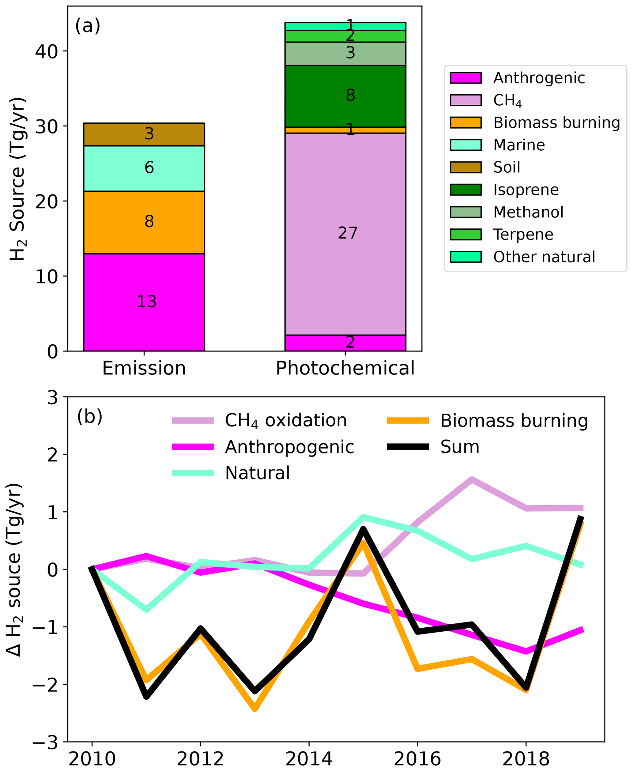
Figure 1Global source of H2 (a) and changes in the magnitude of H2 sources over the 2010–2019 period (b). For clarity, the green line denotes the combined change in H2 emissions and photochemical production from natural sources (marine and soil emissions + BVOCs photooxidation).
Overall, we find that CH4 oxidation is the largest photochemical source of H2 (≃ 27 Tg yr−1). The oxidation of biogenic VOCs (BVOCs) accounts for the majority of the remaining photochemical source of H2 (≃14 Tg yr−1) primarily from isoprene (8 Tg yr−1), methanol (3 Tg yr−1), and terpene (1.5 Tg yr−1). The oxidation of VOCs from anthropogenic and biomass burning origin produces ≃ 3 Tg yr−1 of H2. Our estimates are in good agreement with previous estimates (Ehhalt and Rohrer, 2009): CH4 (23±8 Tg yr−1), isoprene (9±6 Tg yr−1), biomass burning and anthropogenic VOCs (3 Tg yr−1). This similarity can be attributed to the similar yield of H2 from CH2O (0.4 mol mol−1 compared to 0.37; Ehhalt and Rohrer, 2009). More work is needed to better characterize the temperature and pressure sensitivity of CH2O photolysis quantum yields (Röth and Ehhalt, 2015).
Figure 1a summarizes the simulated sources of H2 associated with photochemical production and direct emissions in the BASE run. Over the 2010–2019 period, the average global simulated source of H2 is 74 ± 1 Tg yr−1, with 60 % from photochemical production. Anthropogenic activities are estimated to account for ≃ 40 % of the overall H2, primarily from CH4 oxidation. Note that we assume that 50 % of the photochemical production of H2 from CH4 oxidation is anthropogenic based on the detailed bottom–up inventory of CH4 sources (Saunois et al., 2020). Top–down estimates suggest a higher contribution of anthropogenic sources (≃ 60 %; Saunois et al., 2020), which would further increase the fraction of H2 associated with anthropogenic activities. Figure 1b shows that the simulated total source of H2 changes little over the 2010–2019 period. The simulated annual photochemical source of H2 (excluding non-methane VOCs from biomass burning and anthropogenic origins) is 1.6 Tg yr−1 greater during 2017–2019 than during 2010–2012, with 70 % of this increase attributed to CH4. By contrast, H2 associated with anthropogenic activities decreases (−1.3 Tg yr−1, Fig. S2a), mostly from transport (−1 Tg yr−1) and industries (−0.4 Tg yr−1). The decrease in H2 emissions reflects the decline in CO emissions from these sectors. The interannual variability of the overall H2 source during the 2010–2019 period is dominated by the variability of biomass burning emissions, which can result in interannual changes of ≃2 Tg yr−1.
H2 sinks include chemical oxidation by OH and O(1D) and soil uptake associated with microbial activity. The deposition velocity of H2 (vd(H2)) over land is calculated following the parameterization of Ehhalt and Rohrer (2013) and depends on temperature, soil moisture (Ehhalt and Rohrer, 2013), and soil carbon (Khdhiri et al., 2015; Paulot et al., 2021). In the BASE configuration we use a monthly climatology of vd(H2) calculated using monthly meteorological and soil outputs from the GFDL Earth System Model ESM4.1 over the 1989–2014 period (Dunne et al., 2020; Paulot et al., 2021). Soil uptake is estimated to account for 71 % of the overall H2 sink. The overall lifetime of H2 in the BASE configuration is 2.5 years. The lifetime of H2 associated with anthropogenic emissions is 6 % shorter due to their geographical distribution.
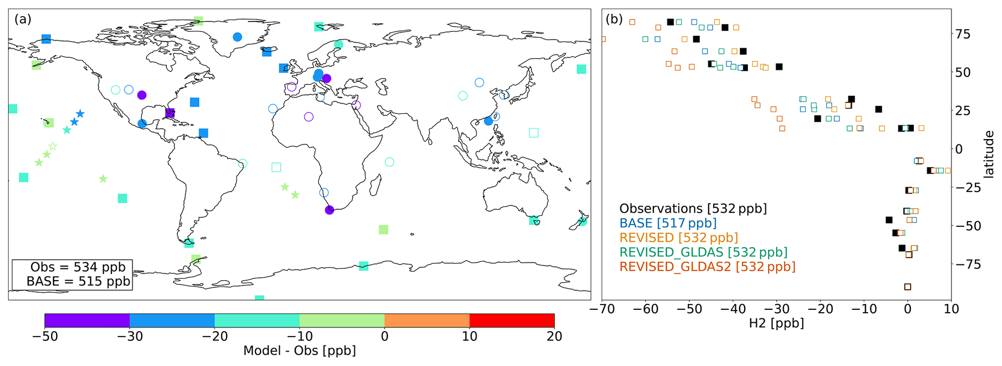
Figure 2Mean model bias at individual sites for the BASE model configuration (a) over the 2010–2019 period. Filled symbols denote sites where the correlation between observed and simulated H2 concentrations exceeds 0.5. Squares and stars denote background sites and cruises, respectively. (b) Observed and simulated difference in H2 at background sites relative to H2 mole fraction measured at the South Pole Observatory. The average concentrations at background sites are indicated for each configuration in the legend.
2.2.2 Sensitivity simulations
In this section, we describe additional model simulations that are designed to explore the impact of uncertainties in the representation of H2 emissions and deposition on the simulation of atmospheric H2 (Table 1). We focus on H2 emissions and deposition as their representations in models are largely derived from limited observational constraints (Derwent et al., 2023; Paulot et al., 2021).
(Paulot et al., 2021)Bertagni et al. (2021)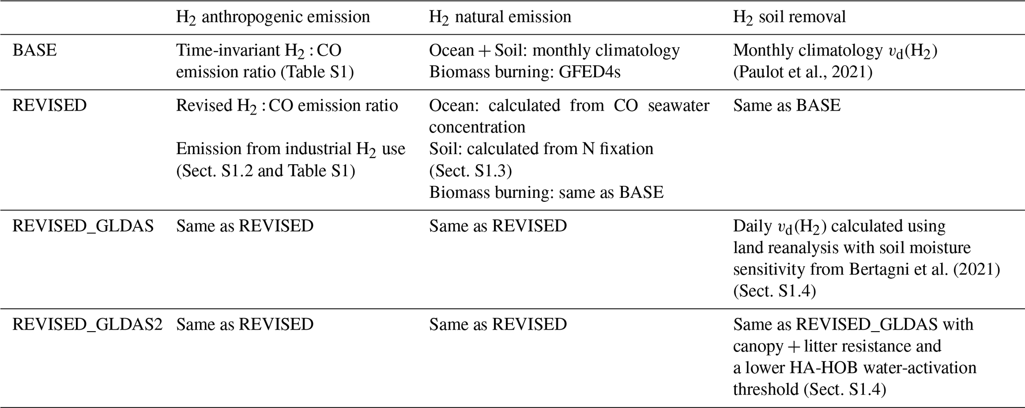
The REVISED configuration focuses on the representation of anthropogenic and natural H2 emissions. The development of the REVISED emission inventory is guided by the biases of the BASE configuration against H2 observations (Sect. S1.1 in the Supplement, Ghosh et al., 2015). In particular, we focus on the representation of transportation emissions (Table S1) and emissions associated with industrial H2 use for refining and ammonia, methanol, and steel production. Further details regarding the treatment of anthropogenic and natural sources in the REVISED emission inventory can be found in the Supplement (Sects. S1.2 and S1.3).
We further consider the impact of a different representation of H2 soil uptake on the simulation of H2. Here, we use the parameterization of the soil moisture response of HA-HOB activity recently developed by Bertagni et al. (2021). This parameterization relates the minimum soil moisture required for H2 uptake by HA-HOB to soil hydrological properties, which facilitates its incorporation into global models. This model also allows us to vary the strength of the diffusion barrier associated with soil litter, which can reduce H2 transport to active sites (Smith-Downey et al., 2008; Ehhalt and Rohrer, 2009). To quantify possible changes in vd(H2) over the 2010–2019 period, we calculate daily deposition velocity using 3-hourly soil moisture, soil temperature, and snow cover from the NASA Global Land Data Assimilation System (Rodell et al., 2004). We focus on two different configurations. In REVISED_GLDAS, we neglect the litter resistance and assume that HA-HOB activity is inhibited when the soil matrix potential (Ψws) is less than the wilting point of plants in semiarid environments (Ψws= −3000 kPa), as recommended by Bertagni et al. (2021). The required soil moisture for the H2 uptake is not well known and experimental studies have shown that HA-HOB are present in very arid environments (Jordaan et al., 2020). In REVISED_GLDAS2, we assume a much lower activation threshold for HA-HOB (Ψws= −10 000 kPa) and account for the litter barrier. Note that both these configurations use the REVISED emission inventory. More details regarding the calculation of vd(H2) can be found in the Supplement (Sect. S1.4).
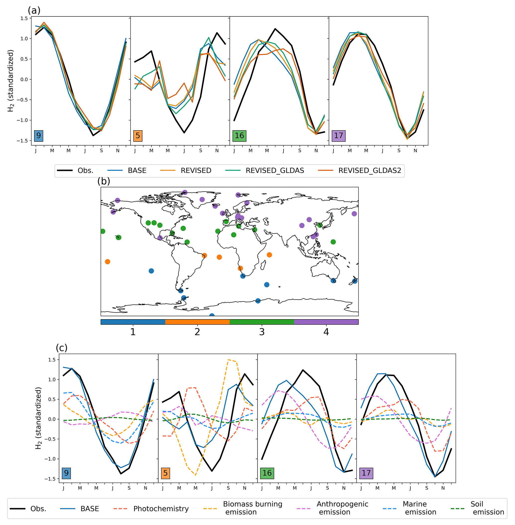
Figure 3Monthly standardized H2 concentration for each cluster (a). The number of sites in each cluster is indicated by insets. The sites included in each cluster are shown in panel (b). The variation of source-tagged H2 tracers in each cluster is shown in panel (c). Source-tagged H2 tracers are normalized using the standard deviation of simulated H2.
3.1 BASE model evaluation
3.1.1 Climatology
Figure 2 shows the average model bias against surface observations from NOAA GML. In the BASE configuration, AM4.1 underestimates H2 at all stations, with greater biases over continental regions (Fig. 2). Correlations exceed 0.5 at more than 90 % of the background sites (squares) but only at 55 % of continental sites. Figure 2b further shows that the concentration at the South Pole is ≃ 50 ppb greater than at the North Pole, which is well captured by the BASE configuration.
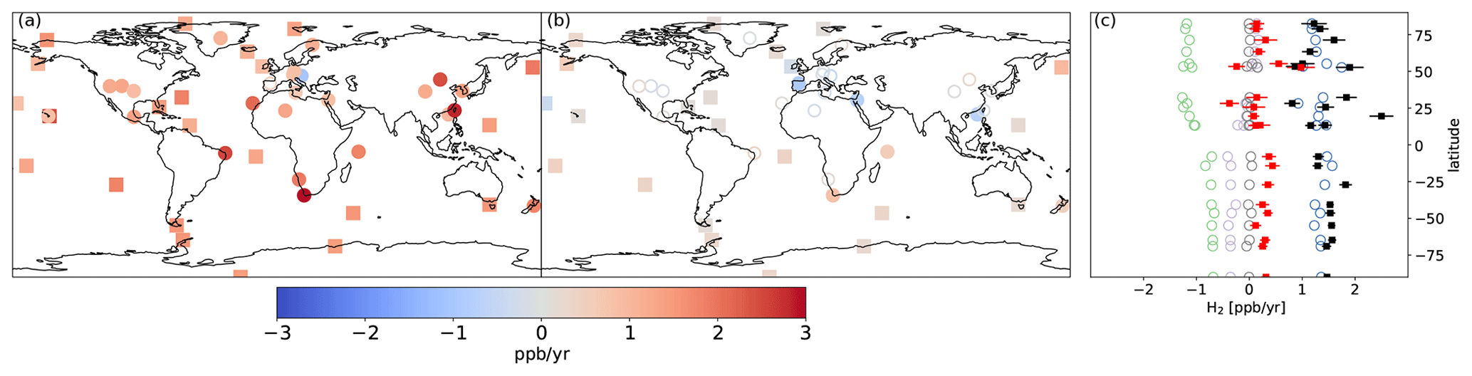
Figure 4Trend in H2 concentrations in observations (a) and in the BASE simulation (b) over the 2010–2019 period. (c) Observed (black) and simulated (red) trend in H2 at background sites (squares) as well as the trend in tagged H2 tracers associated with anthropogenic sources (green), biomass burning (purple), ocean and soil sources (black), and photochemical production (blue). Filled symbols denote trends that are significantly different from 0 (p<0.01). The error bars show 1 SD for the estimated observed and simulated trends.
To examine differences between the model and the observed seasonality, we first apply the Kmean clustering algorithm (Arthur and Vassilvitskii, 2007) to the observed H2 monthly climatology. Since our focus is on the seasonality of H2, we transform the monthly climatology of H2 at each site such that it has a mean of 0 and a standard deviation of 1. Using the within-cluster sum of squares and the silhouette score, we find that the standardized H2 observations can be well represented using four clusters. Figure 3 shows the seasonality of the standardized H2 concentration for each cluster (Fig. 3a) and their spatial distribution (Fig. 3b). Sites are found to cluster broadly by latitude based on the seasonality of H2 with clusters 1, 2, 3, and 4 comprising primarily sites located in the southern mid-to-high latitudes, southern tropics, northern subtropics, and northern mid-to-high latitudes, respectively. The model captures the seasonality of H2 well in the Southern Hemisphere (cluster 1) but peaks 1–3 months earlier than observations for clusters 2, 3, and 4. Figure 3c shows the contribution of different sources of H2 to the simulated seasonality of H2 (inferred from the tagged H2 tracers). The seasonal bias for cluster 2 is primarily driven by H2 emitted from biomass burning, which peaks ∼ 2 months earlier than observations. This delay may be associated with greater burning of woody material toward the end of the dry season, emitting more incompletely oxidized products such as H2 (van der Werf et al., 2006). Figure 3c also shows that the seasonal bias in clusters 3 and 4 may be associated with H2 emitted by anthropogenic activities. As we show in Sect. 3.2.2, this seasonal bias may also reflect errors in the removal of H2.
3.1.2 Time series
Figure 4 shows that H2 has increased at most sites with an average trend at the background sites of 1.4 ± 0.7 ppb yr−1 over the 2010–2019 period with little variability with latitude. Trends are calculated using ordinary least-square regression applied to the de-seasonalized monthly H2 concentrations. By contrast, the simulated H2 concentration in the BASE configuration changes little over this time period.
In the Northern Hemisphere, the lack of a trend at background sites in the model (Fig. 4c) reflects the near-cancellation between the increase of photochemically produced H2 and the decrease in H2 emitted from anthropogenic sources, consistent with the changes in anthropogenic emissions and the photochemical source of H2 from the oxidation of CH4 and biogenic VOCs (Fig. 1). The simulated absolute trend in anthropogenic H2 is ≃ 50 % lower in the Southern Hemisphere relative to the Northern Hemisphere due to the higher relative areal density of anthropogenic sources in the Northern Hemisphere. By contrast, the change in photochemically produced H2 exhibits little variability with latitude and matches the observed trend well. The simulated trend also shows little latitudinal variation due to a decrease in H2 from biomass burning in the Southern Hemisphere.
3.2 Sensitivity simulations
In this section, we explore how uncertainties in the representation of H2 emissions and deposition contribute to the biases in the BASE model run.
3.2.1 Emissions
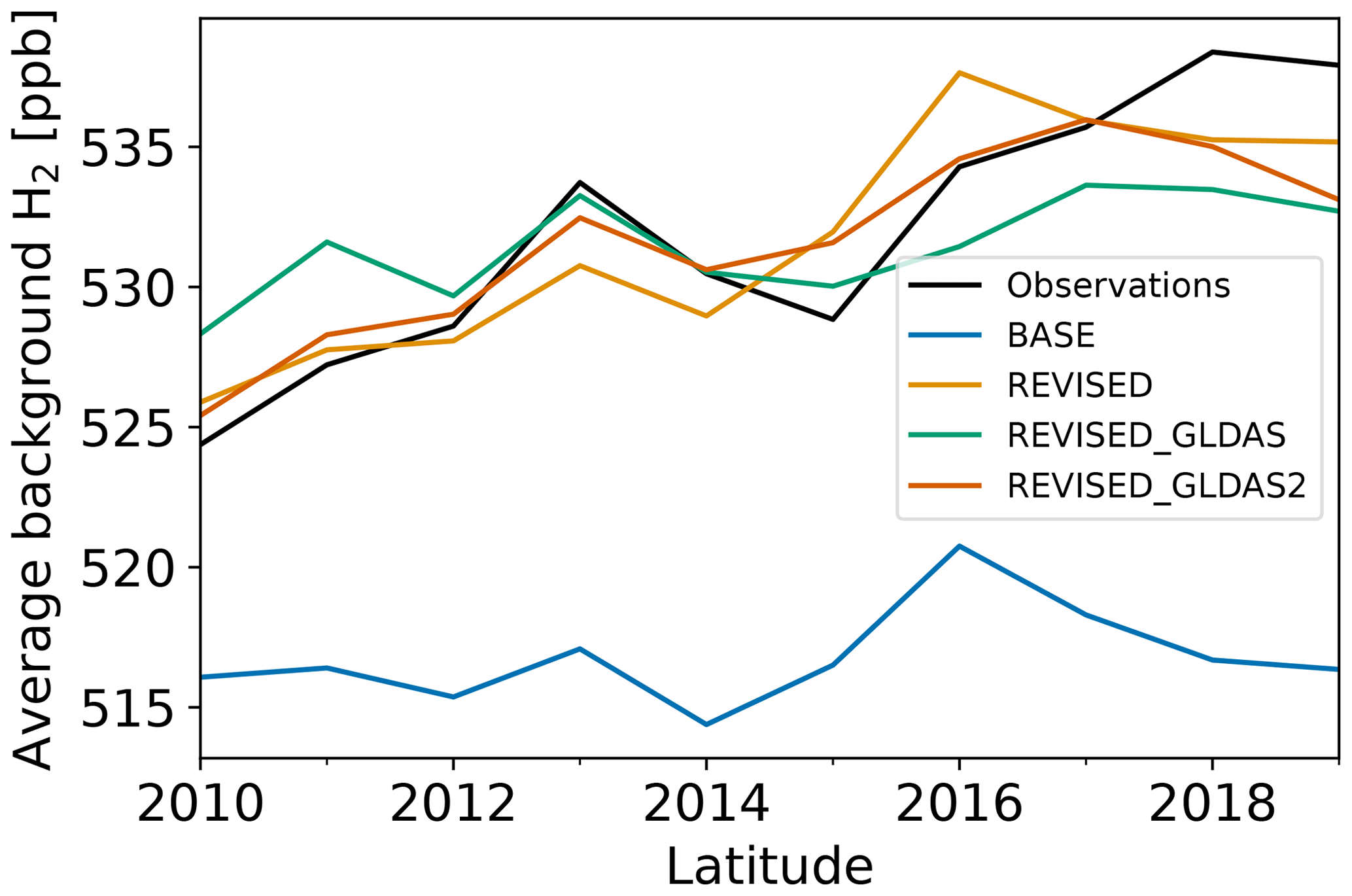
Figure 5 shows that the BASE run exhibits a 10–15 ppb negative bias and fails to capture the ≃ 15 ppb increase over the 2010–2019 period (Fig. 5). From this bias, we estimate a missing source of H2 of ≃ 2–2.5 Tg yr−1 in circa 2010 and 3–4 Tg yr−1 in circa 2019 (Sect. S1.1). Similarly, Derwent et al. (2023) recently reported that a missing H2 source (5 Tg yr−1 in 2020) was required to explain the observed increase in H2 concentration at Mace Head and Cape Grim since 2010.
Figures 5 and 6 show that the observed increase in H2 can be well captured with the REVISED emission inventory. In this inventory, the increase in the missing source of H2 is explained by a lower decrease in anthropogenic H2 emissions associated with fossil fuel combustion (0.9 Tg yr−1 lower in 2019 relative to 2010 compared to 1.6 Tg yr−1 in the BASE inventory) and an increase in H2 emissions associated with H2 industrial usage (0.3 Tg yr−1). We also increase the H2 soil source from 3 to 4.5 Tg yr−1 to reduce the model negative bias. This change is well within the large uncertainties in the minor H2 sources surveyed by Ehhalt and Rohrer (2009). In particular, it is a small fraction of the estimated geological source of H2 (23 ±7 Tg yr−1, Zgonnik, 2020), which we do not account for here.
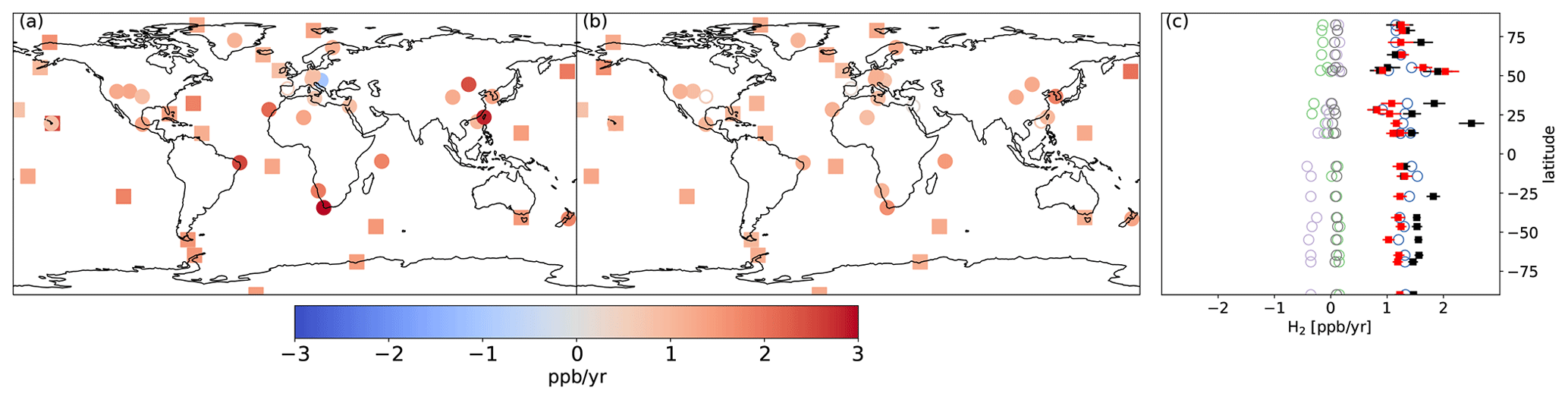
Figure 6Same as Fig. 4 but for the REVISED configuration.
The REVISED emission inventory provides a possible explanation for the observed increase in atmospheric H2. It highlights the importance of constraining H2 emissions associated with H2 industrial use, a sector that is expected to grow rapidly in coming decades.
3.2.2 Deposition
The BASE and REVISED experiments assume no interannual variability in vd(H2). However, we have recently shown that climate change may cause an increase in vd(H2) (Paulot et al., 2021). A recent analysis of observations at Mace Head also suggests that vd(H2) has increased in the past few decades (Derwent et al., 2021).
Figure 7 shows that the REVISED_GLDAS and REVISED_GLDAS2 vd(H2) exhibit different meridional distributions relative to the BASE configuration with faster removal in the subtropics and northern high latitudes but slower removal in the tropics. This reflects more efficient removal of H2 in arid regions and slower removal in the tropics. These spatial differences are the largest for the REVISED_GLDAS2 configuration due to the activation of HA-HOB at a lower soil moisture. Figure 7b further shows that the values of vd(H2) in the REVISED_GLDAS and in the REVISED_GLDAS2 configuration both increase over the 2010–2019 period in the northern midlatitudes. This increase reflects drier and warmer conditions in Europe and the Western US as well as parts of Siberia, which result in faster biological uptake rates and promote H2 diffusivity (Fig. S5). This mechanism may contribute to the reported 1.2 % yr−1 increase in H2 deposition velocity at Mace Head from 1994 to 2020 (Derwent et al., 2021). Drier conditions in Australia trigger biotic limitations, which results in a large decrease in H2 deposition velocity in the southern midlatitudes in the REVISED_GLDAS configuration. By contrast, we find no significant suppression of H2 uptake in Australia over this time period in the REVISED_GLDAS2 configuration due a lower threshold for biotic limitations.
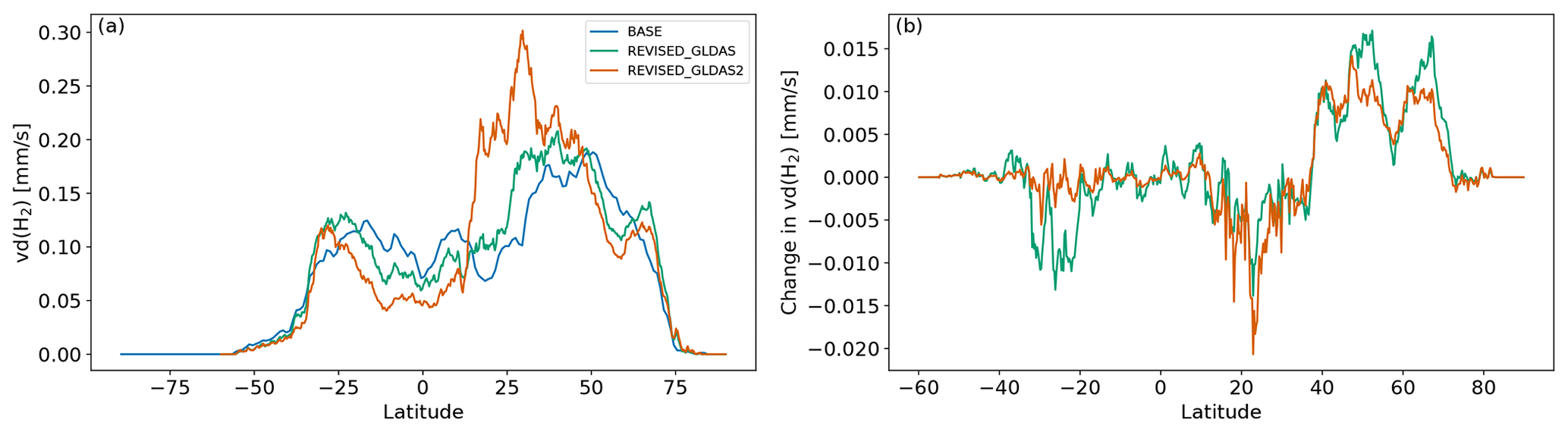
Figure 7Meridional distribution of vd(H2) in the BASE, REVISED_GLDAS, and REVISED_GLDAS2 simulations (a) and (b) simulated change in vd(H2) between the periods 2017–2019 and 2010–2012.
Changes to the spatial distribution of vd(H2) and the increase in H2 removal in the northern midlatitudes (Fig. 7b) in REVISED_GLDAS result in a larger pole-to-pole difference in surface H2 (Fig. 2) and a reduction in the simulated trend (Fig. 8) in the northern mid-to-high latitudes. Both of these changes tend to degrade the model performance relative to the REVISED configuration. By contrast, the REVISED_GLDAS configuration better captures the timing of the H2 maximum in the Northern Hemisphere (clusters 3 and 4, Fig. 3a).
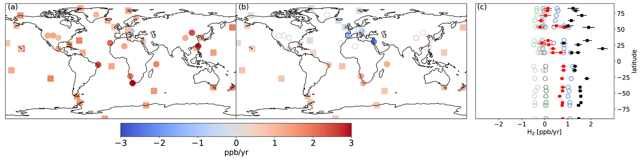
Figure 8Same as Fig. 4 but for the REVISED_GLDAS configuration.
Figure 9 shows the systematic assessment of the sensitivity of vd(H2) to Ψws and the strength of the litter barrier. We find that a lower soil moisture threshold for HA-HOB activation (i.e., a lower Ψws) favors H2 removal in the Northern Hemisphere relative to the Southern Hemisphere (Fig. 9a) and results in a larger increase in vd(H2) over the 2010–2019 period (Fig. 9b), especially in the Southern Hemisphere (Fig. 9c). This suggests that a lower Ψws would tend to worsen the model performance in the absence of a litter barrier (given the REVISED emissions). The litter barrier tends to increase the importance of arid regions for H2 removal. This makes H2 uptake more susceptible to moisture inhibition, such that a stronger litter barrier tends to result in a lower increase or even a decrease in vd(H2) over the 2010–2019 period. Under all scenarios, the litter barrier tends to increase the gradient in vd(H2) between the Northern Hemisphere and the Southern Hemisphere.
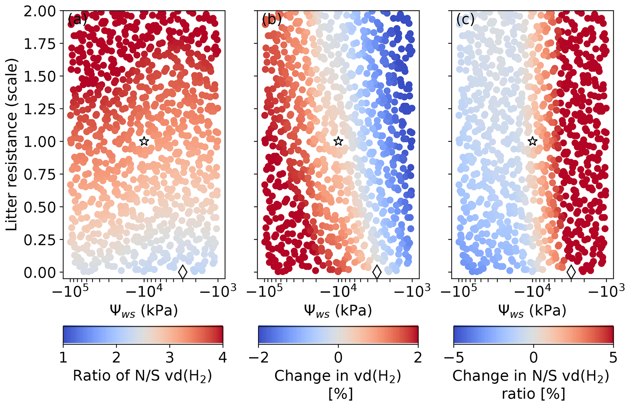
Figure 9Simulated sensitivity of vd(H2) to Ψws and the strength of the litter diffusive barrier. Panel (a) shows the response of the ratio of vd(H2). Panel (b) shows the change in vd(H2) between 2010–2012 and 2017–2019. Panel (c) shows the change in the north/south ratio of vd(H2) between 2010–2012 and 2017–2019. The REVISED_GLDAS configuration uses Ψws= −3000 kPa and no litter resistance (diamond). The REVISED_GLDAS2 uses Ψws= −10 000 kPa and the default (scale = 1) litter resistance (star). The litter scale reflects the perturbation to the default litter resistance (see Sect. S1.4).
It is notable that no configuration results in a small change in vd(H2) without producing large and increasing gradients between the Northern Hemisphere and Southern Hemisphere. As a result, our model cannot capture the observed trends, meridional gradient, and seasonality together given our REVISED estimate of H2 emissions. This is illustrated by the REVISED_GLDAS2 configuration (Ψws = −10 000 kPa, litter_scale = 1), which is found to improve the simulated trend relative to the REVISED_GLDAS (not shown) and the simulated seasonality relative to the REVISED configuration (Fig. 3) but results in a large overestimate of the hemispheric gradient (Fig. 2). This highlights the need for a more detailed representation of the factors that modulate vd(H2) (Khdhiri et al., 2015) to help interpret changes in H2 concentrations.
The recently released H2 dry air mole fraction measurements from the NOAA Global Cooperative Air Sampling Network expand the spatial coverage of the WMO Global Atmospheric Watch observations. This offers the opportunity to assess the representation of the H2 atmospheric budget in the state-of-the-art GFDL-AM4.1 global atmospheric chemistry-climate model. Observations show that H2 has increased on average by 1–2 ppb yr−1 over the 2010–2019 period. This change can be explained by the increase in photochemically produced H2 (mostly from CH4), provided direct anthropogenic H2 emissions have remained stable during this time period. We hypothesize that this stability reflects the compensation between declining emissions associated with fossil fuel combustion (mostly from the transport sector) and increasing emissions associated with H2-producing facilities (for refining and ammonia, methanol, and steel production). This is notable since H2 release from H2 production facilities is poorly understood yet important for assessing the climate benefits of H2 (Hauglustaine et al., 2022; Bertagni et al., 2022).
We show that the observed trend, seasonality, and meridional gradient of H2 provide complementary constraints on the global H2 biogeochemical cycle. We find that our model fails to capture all three constraints together, which most likely reflects fundamental gaps in our representation of the soil removal of H2 by microorganisms (HA-HOB). Such uncertainties are important, as an increase in vd(H2) would require a commensurate increase in H2 sources to explain the observed change in H2 concentration.
This study highlights the need for coordinated field and laboratory data collection efforts to help improve models of the distribution and activity of HA-HOB in global models (American Academy of Microbiology, 2023). Such work is critical for quantifying the response of atmospheric H2 to increasing anthropogenic H2 usage as well as hydrological changes associated with climate change (Jansson and Hofmockel, 2019; Huang et al., 2015); however, it is hindered by the lack of sensors that offer higher time resolution and maintain good sensitivity and stable response.
The code for the GFDL ESM4.1 model is available at https://doi.org/10.5281/zenodo.5347705 (Robinson, 2021). NOAA Global Cooperative Network Flask Air H2 (Pétron et al., 2023) can be downloaded at https://doi.org/10.15138/WP0W-EZ08.
The supplement related to this article is available online at: https://doi.org/10.5194/acp-24-4217-2024-supplement.
FP designed the research and developed and analyzed the model simulations. GP and AC collected and processed H2 observations from the NOAA network and provided guidance regarding their interpretation. MB developed the soil moisture parameterization of HA-HOB used in the REVISED_GLDAS and REVISED_GLDAS2 configurations. All authors contributed to the drafting of the manuscript.
The contact author has declared that none of the authors has any competing interests.
The views expressed in this paper do not necessarily represent the views of the US Department of Energy or the United States Government.
Publisher’s note: Copernicus Publications remains neutral with regard to jurisdictional claims made in the text, published maps, institutional affiliations, or any other geographical representation in this paper. While Copernicus Publications makes every effort to include appropriate place names, the final responsibility lies with the authors.
We thank Vaishali Naik for her help with generating model-ready H2 emissions. We thank Larry Horowitz, Vaishali Naik, Amilcare Porporato, and Xinning Zhang for their helpful comments on the paper.
This research has been supported in part by NOAA cooperative agreements NA17OAR4320101 and NA22OAR4320151 and by the US Department of Energy, Office of Energy Efficiency and Renewable Energy (EERE), specifically the Hydrogen and Fuel Cell Technologies Office.
This paper was edited by Manvendra Krishna Dubey and reviewed by two anonymous referees.
Abe, J., Popoola, A., Ajenifuja, E., and Popoola, O.: Hydrogen energy, economy and storage: Review and recommendation, Int. J. Hydrogen Energ., 44, 15072–15086, https://doi.org/10.1016/j.ijhydene.2019.04.068, 2019. a
Akagi, S. K., Yokelson, R. J., Wiedinmyer, C., Alvarado, M. J., Reid, J. S., Karl, T., Crounse, J. D., and Wennberg, P. O.: Emission factors for open and domestic biomass burning for use in atmospheric models, Atmos. Chem. Phys., 11, 4039–4072, https://doi.org/10.5194/acp-11-4039-2011, 2011. a
American Academy of Microbiology: Microbes in Models: Integrating Microbes into Earth System Models for Understanding Climate Change: Report on an American Academy of Microbiology Virtual Colloquium, Washington, D.C., 6 and 8 December 2022, https://asm.org/reports/microbes-in-models-integrating-microbes-into-earth (last access: 9 June 2023), 2023. a
Andreae, M. O.: Emission of trace gases and aerosols from biomass burning – an updated assessment, Atmos. Chem. Phys., 19, 8523–8546, https://doi.org/10.5194/acp-19-8523-2019, 2019. a
Arthur, D. and Vassilvitskii, S.: K-means: The advantages of careful seeding, Proceedings of the eighteenth annual ACM-SIAM symposium on discreate algorithm, New Orleans, Louisiana, 7 January 2007, https://dl.acm.org/doi/10.5555/1283383.1283494 (last access: 5 April 2024), 2007. a
Bay, S. K., Dong, X., Bradley, J. A., Leung, P. M., Grinter, R., Jirapanjawat, T., Arndt, S. K., Cook, P. L. M., LaRowe, D. E., Nauer, P. A., Chiri, E., and Greening, C.: Trace gas oxidizers are widespread and active members of soil microbial communities, Nat. Microbiol., 6, 246–256, https://doi.org/10.1038/s41564-020-00811-w, 2021. a
Bertagni, M. B., Paulot, F., and Porporato, A.: Moisture Fluctuations Modulate Abiotic and Biotic Limitations of H2 Soil Uptake, Global Biogeochem. Cy., 35, e2021GB006987, https://doi.org/10.1029/2021gb006987, 2021. a, b, c, d
Bertagni, M. B., Pacala, S. W., Paulot, F., and Porporato, A.: Risk of the hydrogen economy for atmospheric methane, Nat. Commun., 13, 7706, https://doi.org/10.1038/s41467-022-35419-7, 2022. a, b
Constant, P., Poissant, L., and Villemur, R.: Isolation of Streptomyces sp. PCB7, the first microorganism demonstrating high-affinity uptake of tropospheric H2, The ISME Journal, 2, 1066–1076, https://doi.org/10.1038/ismej.2008.59, 2008. a
da Silva Veras, T., Mozer, T. S., da Costa Rubim Messeder dos Santos, D., and da Silva César, A.: Hydrogen: Trends, production and characterization of the main process worldwide, Int. J. Hydrogen Energ., 42, 2018–2033, https://doi.org/10.1016/j.ijhydene.2016.08.219, 2017. a
Dawood, F., Anda, M., and Shafiullah, G.: Hydrogen production for energy: An overview, Int. J. Hydrogen Energ., 45, 3847–3869, https://doi.org/10.1016/j.ijhydene.2019.12.059, 2020. a
Derwent, R. G., Collins, W. J., Johnson, C. E., and Stevenson, D. S.: Transient Behaviour of Tropospheric Ozone Precursors in a Global 3-D CTM and Their Indirect Greenhouse Effects, Clim. Change, 49, 463–487, https://doi.org/10.1023/a:1010648913655, 2001. a
Derwent, R. G., Simmonds, P. G., Doherty, S. J. O., Spain, T. G., and Young, D.: Natural greenhouse gas and ozone-depleting substance sources and sinks from the peat bogs of Connemara, Ireland from 1994–2020, Environmental Science Atmospheres, 1, 406–415, https://doi.org/10.1039/d1ea00040c, 2021. a, b, c
Derwent, R. G., Simmonds, P. G., O'Doherty, S., Manning, A. J., and Spain, T. G.: High-frequency, continuous hydrogen observations at Mace Head, Ireland from 1994 to 2022: Baselines, pollution events and “missing” sources, Atmos. Environ., 312, 120029, https://doi.org/10.1016/j.atmosenv.2023.120029, 2023. a, b, c
Dunne, J. P., Horowitz, L. W., Adcroft, A. J., Ginoux, P., Held, I. M., John, J. G., Krasting, J. P., Malyshev, S., Naik, V., Paulot, F., Shevliakova, E., Stock, C. A., Zadeh, N., Balaji, V., Blanton, C., Dunne, K. A., Dupuis, C., Durachta, J., Dussin, R., Gauthier, P. P. G., Griffies, S. M., Guo, H., Hallberg, R. W., Harrison, M., He, J., Hurlin, W., McHugh, C., Menzel, R., Milly, P. C. D., Nikonov, S., Paynter, D. J., Ploshay, J., Radhakrishnan, A., Rand, K., Reichl, B. G., Robinson, T., Schwarzkopf, D. M., Sentman, L. T., Underwood, S., Vahlenkamp, H., Winton, M., Wittenberg, A. T., Wyman, B., Zeng, Y., and Zhao, M.: The GFDL Earth System Model version 4.1 (GFDL-ESM 4.1): Overall coupled model description and simulation characteristics, J. Adv. Model. Earth Sy., e2019MS002015, https://doi.org/10.1029/2019ms002015, 2020. a
Ehhalt, D. and Rohrer, F.: Deposition velocity of H2: a new algorithm for its dependence on soil moisture and temperature, Tellus B, 65, 19904, https://doi.org/10.3402/tellusb.v65i0.19904, 2013. a, b, c
Ehhalt, D. H. and Rohrer, F.: The tropospheric cycle of H2: a critical review, Tellus B, 61, 500–535, https://doi.org/10.1111/j.1600-0889.2009.00416.x, 2009. a, b, c, d, e, f, g, h
Francey, R. J., Steele, L. P., Spencer, D. A., Langenfelds, R. L., Law, R. M., Krummel, P. B., Fraser, P. J., Etheridge, D. M., Derek, N., Coram, S. A., Cooper, L. N., Allison, C. E., Porter, L., and Baly, S.: The CSIRO (Australia) measurement of greenhouse gases in the global atmosphere, Tech. rep., http://hdl.handle.net/102.100.100/191835?index=1 (last access: 26 June 2020), 2003. a
Ghosh, A., Patra, P. K., Ishijima, K., Umezawa, T., Ito, A., Etheridge, D. M., Sugawara, S., Kawamura, K., Miller, J. B., Dlugokencky, E. J., Krummel, P. B., Fraser, P. J., Steele, L. P., Langenfelds, R. L., Trudinger, C. M., White, J. W. C., Vaughn, B., Saeki, T., Aoki, S., and Nakazawa, T.: Variations in global methane sources and sinks during 1910–2010, Atmos. Chem. Phys., 15, 2595–2612, https://doi.org/10.5194/acp-15-2595-2015, 2015. a
Global Monitoring Laboratory: Carbon Cycle Gases observation sites, https://www.gml.noaa.gov/dv/site/?program=ccgg (last access: 1 January 2024), 2023. a
Granier, C., Lamarque, J. F., Mieville, A., Müller, J. F., Olivier, J., Orlando, J., Peters, J., Petron, G., Tyndall, G., and Wallens, S.: POET, a database of surface emissions of ozone precursors, Tech. rep., http://www.aero.jussieu.fr/projet/ACCENT/POET.php (last access: 28 December 2020), 2005. a, b
Grant, A., Archibald, A. T., Cooke, M. C., Nickless, G., and Shallcross, D. E.: Modelling the oxidation of 15 VOCs to track yields of hydrogen, Atmos. Sci. Lett., 11, 265–269, https://doi.org/10.1002/asl.286, 2010. a
Greening, C. and Grinter, R.: Microbial oxidation of atmospheric trace gases, Nat. Rev. Microbiol., 20, 513–528, https://doi.org/10.1038/s41579-022-00724-x, 2022. a
Greening, C., Constant, P., Hards, K., Morales, S. E., Oakeshott, J. G., Russell, R. J., Taylor, M. C., Berney, M., Conrad, R., and Cook, G. M.: Atmospheric Hydrogen Scavenging: from Enzymes to Ecosystems, Appl. Environ. Microb., 81, 1190–1199, https://doi.org/10.1128/aem.03364-14, 2015. a
Guenther, A. B., Jiang, X., Heald, C. L., Sakulyanontvittaya, T., Duhl, T., Emmons, L. K., and Wang, X.: The Model of Emissions of Gases and Aerosols from Nature version 2.1 (MEGAN2.1): an extended and updated framework for modeling biogenic emissions, Geosci. Model Dev., 5, 1471–1492, https://doi.org/10.5194/gmd-5-1471-2012, 2012. a
Hauglustaine, D., Paulot, F., Collins, W., Derwent, R., Sand, M., and Boucher, O.: Climate benefit of a future hydrogen economy, Commun. Earth Environ., 3, 295, https://doi.org/10.1038/s43247-022-00626-z, 2022. a, b, c
Holladay, J., Hu, J., King, D., and Wang, Y.: An overview of hydrogen production technologies, Catal. Today, 139, 244–260, https://doi.org/10.1016/j.cattod.2008.08.039, 2009. a
Horowitz, L. W., Naik, V., Paulot, F., Ginoux, P. A., Dunne, J. P., Mao, J., Schnell, J., Chen, X., He, J., John, J. G., Lin, M., Lin, P., Malyshev, S., Paynter, D., Shevliakova, E., and Zhao, M.: The GFDL Global Atmospheric Chemistry-Climate Model AM4.1: Model Description and Simulation Characteristics, J. Adv. Model. Earth Sy., e2019MS002032, https://doi.org/10.1029/2019ms002032, 2020. a, b
Howarth, R. W. and Jacobson, M. Z.: How green is blue hydrogen?, Energy Sci. Eng., 9, 1676–1687, https://doi.org/10.1002/ese3.956, 2021. a, b
Huang, J., Yu, H., Guan, X., Wang, G., and Guo, R.: Accelerated dryland expansion under climate change, Nat. Clim. Change, 6, 166–171, https://doi.org/10.1038/nclimate2837, 2015. a
Hydrogen Council: Hydrogen scaling up. A sustainable pathway for the global energy transition, Hydrogen Council, https://hydrogencouncil.com/wp-content/uploads/2017/11/Hydrogen-Scaling-up_Hydrogen-Council_2017.compressed.pdf (last access: 29 March 2024), 2017. a
International Energy Agency: The Future of Hydrogen – Seizing today's opportunities, Tech. rep., International Energy Agency, Paris, France, https://www.iea.org/reports/the-future-of-hydrogen (last access: 29 March 2024), 2019. a
International Energy Agency: Global Hydrogen Review 2022, Tech. rep., International Energy Agency, Paris, France, https://www.iea.org/reports/global-hydrogen-review-2022 (last access: 29 March 2024), 2022. a
Jansson, J. K. and Hofmockel, K. S.: Soil microbiomes and climate change, Nat. Rev. Microbiol., 18, 35–46, https://doi.org/10.1038/s41579-019-0265-7, 2019. a
Jordaan, K., Lappan, R., Dong, X., Aitkenhead, I. J., Bay, S. K., Chiri, E., Wieler, N., Meredith, L. K., Cowan, D. A., Chown, S. L., and Greening, C.: Hydrogen-Oxidizing Bacteria Are Abundant in Desert Soils and Strongly Stimulated by Hydration, mSystems, 5, 01131-20, https://doi.org/10.1128/msystems.01131-20, 2020. a
Jordan, A. and Steinberg, B.: Calibration of atmospheric hydrogen measurements, Atmos. Meas. Tech., 4, 509–521, https://doi.org/10.5194/amt-4-509-2011, 2011. a
Kalnay, E., Kanamitsu, M., Kistler, R., Collins, W., Deaven, D., Gandin, L., Iredell, M., Saha, S., White, G., Woollen, J., Zhu, Y., Leetmaa, A., Reynolds, R., Chelliah, M., Ebisuzaki, W., Higgins, W., Janowiak, J., Mo, K. C., Ropelewski, C., Wang, J., Jenne, R., and Joseph, D.: The NCEP/NCAR 40-Year Reanalysis Project, B. Am. Meteorol. Soc., 77, 437–471, 1996. a
Khdhiri, M., Hesse, L., Popa, M. E., Quiza, L., Lalonde, I., Meredith, L. K., Röckmann, T., and Constant, P.: Soil carbon content and relative abundance of high affinity H2-oxidizing bacteria predict atmospheric H2 soil uptake activity better than soil microbial community composition, Soil Biol. Biochem., 85, 1–9, https://doi.org/10.1016/j.soilbio.2015.02.030, 2015. a, b
Lapi, T., Chatzimpiros, P., Raineau, L., and Prinzhofer, A.: System approach to natural versus manufactured hydrogen: An interdisciplinary perspective on a new primary energy source, Int. J. Hydrogen Energ., 47, 21701–21712, https://doi.org/10.1016/j.ijhydene.2022.05.039, 2022. a
Lefeuvre, N., Truche, L., Donzé, F., Ducoux, M., Barré, G., Fakoury, R., Calassou, S., and Gaucher, E. C.: Native H2 Exploration in the Western Pyrenean Foothills, Geochem. Geophy. Geosy., 22, e2021GC009917, https://doi.org/10.1029/2021gc009917, 2021. a
Li, J., Mao, J., Min, K.-E., Washenfelder, R. A., Brown, S. S., Kaiser, J., Keutsch, F. N., Volkamer, R., Wolfe, G. M., Hanisco, T. F., Pollack, I. B., Ryerson, T. B., Graus, M., Gilman, J. B., Lerner, B. M., Warneke, C., de Gouw, J. A., Middlebrook, A. M., Liao, J., Welti, A., Henderson, B. H., McNeill, V. F., Hall, S. R., Ullmann, K., Donner, L. J., Paulot, F., and Horowitz, L. W.: Observational constraints on glyoxal production from isoprene oxidation and its contribution to organic aerosol over the Southeast United States, J. Geophys. Res.-Atmos., 121, 9849–9861, https://doi.org/10.1002/2016JD025331, 2016. a
Meinshausen, M., Vogel, E., Nauels, A., Lorbacher, K., Meinshausen, N., Etheridge, D. M., Fraser, P. J., Montzka, S. A., Rayner, P. J., Trudinger, C. M., Krummel, P. B., Beyerle, U., Canadell, J. G., Daniel, J. S., Enting, I. G., Law, R. M., Lunder, C. R., O'Doherty, S., Prinn, R. G., Reimann, S., Rubino, M., Velders, G. J. M., Vollmer, M. K., Wang, R. H. J., and Weiss, R.: Historical greenhouse gas concentrations for climate modelling (CMIP6), Geosci. Model Dev., 10, 2057–2116, https://doi.org/10.5194/gmd-10-2057-2017, 2017. a
Meinshausen, M., Nicholls, Z. R. J., Lewis, J., Gidden, M. J., Vogel, E., Freund, M., Beyerle, U., Gessner, C., Nauels, A., Bauer, N., Canadell, J. G., Daniel, J. S., John, A., Krummel, P. B., Luderer, G., Meinshausen, N., Montzka, S. A., Rayner, P. J., Reimann, S., Smith, S. J., van den Berg, M., Velders, G. J. M., Vollmer, M. K., and Wang, R. H. J.: The shared socio-economic pathway (SSP) greenhouse gas concentrations and their extensions to 2500, Geosci. Model Dev., 13, 3571–3605, https://doi.org/10.5194/gmd-13-3571-2020, 2020. a
Meredith, L. K., Commane, R., Keenan, T. F., Klosterman, S. T., Munger, J. W., Templer, P. H., Tang, J., Wofsy, S. C., and Prinn, R. G.: Ecosystem fluxes of hydrogen in a mid-latitude forest driven by soil microorganisms and plants, Glob. Change Biol., 23, 906–919, https://doi.org/10.1111/gcb.13463, 2016. a
Milkov, A. V.: Molecular hydrogen in surface and subsurface natural gases: Abundance, origins and ideas for deliberate exploration, Earth-Sci. Rev., 230, 104063, https://doi.org/10.1016/j.earscirev.2022.104063, 2022. a
Ocko, I. B. and Hamburg, S. P.: Climate consequences of hydrogen emissions, Atmos. Chem. Phys., 22, 9349–9368, https://doi.org/10.5194/acp-22-9349-2022, 2022. a
O'Rourke, P., Smith, S., Mott, A., Ahsan, H., Mcduffie, E., Crippa, M., Klimont, Z., Mcdonald, B., Wang, S., Nicholson, M., Hoesly, R., and Feng, L.: CEDS v_2021_04_21 Gridded emissions data, DataHub Pacific Northwest [data set], https://doi.org/10.25584/PNNLDATAHUB/1779095, 2021. a, b
Paulot, F., Paynter, D., Naik, V., Malyshev, S., Menzel, R., and Horowitz, L. W.: Global modeling of hydrogen using GFDL-AM4.1: Sensitivity of soil removal and radiative forcing, Int. J. Hydrogen Energ., 46, 13446–13460, https://doi.org/10.1016/j.ijhydene.2021.01.088, 2021. a, b, c, d, e, f, g, h, i, j
Pétron, G., Crotwell, A., Crotwell, M., Kitzis, D., Madronich, M., Mefford, T., Moglia, E., Mund, J., Neff, D., Thoning, K., and Wolter, S.: Atmospheric Hydrogen Dry Air Mole Fractions from the NOAA GML Carbon Cycle Cooperative Global Air Sampling Network, 2009–2021, Global Monitoring Laboratory [data set], https://doi.org/10.15138/WP0W-EZ08, 2023. a
Pétron, G. B., Crotwell, A. M., Mund, J., Crotwell, M., Mefford, T., Thoning, K., Hall, B. D., Kitzis, D. R., Madronich, M., Moglia, E., Neff, D., Wolter, S., Jordan, A., Krummel, P., Langenfelds, R., and Patterson, J. D.: Atmospheric H2 observations from the NOAA Global Cooperative Air Sampling Network, Atmos. Meas. Tech. Discuss. [preprint], https://doi.org/10.5194/amt-2024-4, in review, 2024. a, b
Price, H., Jaeglé, L., Rice, A., Quay, P., Novelli, P. C., and Gammon, R.: Global budget of molecular hydrogen and its deuterium content: Constraints from ground station, cruise, and aircraft observations, J. Geophys. Res., 112, D22108, https://doi.org/10.1029/2006jd008152, 2007. a
Prinn, R. G., Weiss, R. F., Arduini, J., Arnold, T., DeWitt, H. L., Fraser, P. J., Ganesan, A. L., Gasore, J., Harth, C. M., Hermansen, O., Kim, J., Krummel, P. B., Li, S., Loh, Z. M., Lunder, C. R., Maione, M., Manning, A. J., Miller, B. R., Mitrevski, B., Mühle, J., O'Doherty, S., Park, S., Reimann, S., Rigby, M., Saito, T., Salameh, P. K., Schmidt, R., Simmonds, P. G., Steele, L. P., Vollmer, M. K., Wang, R. H., Yao, B., Yokouchi, Y., Young, D., and Zhou, L.: History of chemically and radiatively important atmospheric gases from the Advanced Global Atmospheric Gases Experiment (AGAGE), Earth Syst. Sci. Data, 10, 985–1018, https://doi.org/10.5194/essd-10-985-2018, 2018. a
Prinzhofer, A., Cissé, C. S. T., and Diallo, A. B.: Discovery of a large accumulation of natural hydrogen in Bourakebougou (Mali), Int. J. Hydrogen Energ., 43, 19315–19326, https://doi.org/10.1016/j.ijhydene.2018.08.193, 2018. a
Rayner, N. A., Parker, D. E., Horton, E. B., Folland, C. K., Alexander, L. V., Rowell, D. P., Kent, E. C., and Kaplan, A.: Global analyses of sea surface temperature, sea ice, and night marine air temperature since the late nineteenth century, J. Geophys. Res.-Atmos., 108, 4407, https://doi.org/10.1029/2002JD002670, 2003. a
Robinson, T.: NOAA-GFDL/ESM4: 2021.03 (2021.03), Zenodo [code], https://doi.org/10.5281/zenodo.5347705, 2021.
Rodell, M., Houser, P. R., Jambor, U., Gottschalck, J., Mitchell, K., Meng, C.-J., Arsenault, K., Cosgrove, B., Radakovich, J., Bosilovich, M., Entin, J. K., Walker, J. P., Lohmann, D., and Toll, D.: The Global Land Data Assimilation System, B. Am. Meteorol. Soc., 85, 381–394, https://doi.org/10.1175/bams-85-3-381, 2004. a
Röth, E.-P. and Ehhalt, D. H.: A simple formulation of the CH2O photolysis quantum yields, Atmos. Chem. Phys., 15, 7195–7202, https://doi.org/10.5194/acp-15-7195-2015, 2015. a
Sand, M., Skeie, R. B., Sandstad, M., Krishnan, S., Myhre, G., Bryant, H., Derwent, R., Hauglustaine, D., Paulot, F., Prather, M., and Stevenson, D.: A multi-model assessment of the Global Warming Potential of hydrogen, Commun. Earth Environ., 4, 203, https://doi.org/10.1038/s43247-023-00857-8, 2023. a
Saunois, M., Stavert, A. R., Poulter, B., Bousquet, P., Canadell, J. G., Jackson, R. B., Raymond, P. A., Dlugokencky, E. J., Houweling, S., Patra, P. K., Ciais, P., Arora, V. K., Bastviken, D., Bergamaschi, P., Blake, D. R., Brailsford, G., Bruhwiler, L., Carlson, K. M., Carrol, M., Castaldi, S., Chandra, N., Crevoisier, C., Crill, P. M., Covey, K., Curry, C. L., Etiope, G., Frankenberg, C., Gedney, N., Hegglin, M. I., Höglund-Isaksson, L., Hugelius, G., Ishizawa, M., Ito, A., Janssens-Maenhout, G., Jensen, K. M., Joos, F., Kleinen, T., Krummel, P. B., Langenfelds, R. L., Laruelle, G. G., Liu, L., Machida, T., Maksyutov, S., McDonald, K. C., McNorton, J., Miller, P. A., Melton, J. R., Morino, I., Müller, J., Murguia-Flores, F., Naik, V., Niwa, Y., Noce, S., O'Doherty, S., Parker, R. J., Peng, C., Peng, S., Peters, G. P., Prigent, C., Prinn, R., Ramonet, M., Regnier, P., Riley, W. J., Rosentreter, J. A., Segers, A., Simpson, I. J., Shi, H., Smith, S. J., Steele, L. P., Thornton, B. F., Tian, H., Tohjima, Y., Tubiello, F. N., Tsuruta, A., Viovy, N., Voulgarakis, A., Weber, T. S., van Weele, M., van der Werf, G. R., Weiss, R. F., Worthy, D., Wunch, D., Yin, Y., Yoshida, Y., Zhang, W., Zhang, Z., Zhao, Y., Zheng, B., Zhu, Q., Zhu, Q., and Zhuang, Q.: The Global Methane Budget 2000–2017, Earth Syst. Sci. Data, 12, 1561–1623, https://doi.org/10.5194/essd-12-1561-2020, 2020. a, b
Smith-Downey, N. V., Randerson, J. T., and Eiler, J. M.: Temperature and moisture dependence of soil H2 uptake measured in the laboratory, Geophys. Res. Lett., 33, L14813, https://doi.org/10.1029/2006gl026749, 2006. a
Smith-Downey, N. V., Randerson, J. T., and Eiler, J. M.: Molecular hydrogen uptake by soils in forest, desert, and marsh ecosystems in California, J. Geophys. Res., 113, G03037, https://doi.org/10.1029/2008jg000701, 2008. a
Staffell, I., Scamman, D., Abad, A. V., Balcombe, P., Dodds, P. E., Ekins, P., Shah, N., and Ward, K. R.: The role of hydrogen and fuel cells in the global energy system, Energ. Environ. Sci., 12, 463–491, https://doi.org/10.1039/c8ee01157e, 2019. a
Taylor, K. E., Williamson, D., and Zwiers, F.: The sea surface temperature and sea-ice concentration boundary conditions for AMIP II simulations, Program for Climate Model Diagnosis and Intercomparison, Lawrence Livermore National Laboratory, University of California, https://pcmdi.llnl.gov/report/ab60.html (last access: 29 March 2024), 2000. a
van der Werf, G. R., Randerson, J. T., Giglio, L., Collatz, G. J., Kasibhatla, P. S., and Arellano Jr., A. F.: Interannual variability in global biomass burning emissions from 1997 to 2004, Atmos. Chem. Phys., 6, 3423–3441, https://doi.org/10.5194/acp-6-3423-2006, 2006. a
van der Werf, G. R., Randerson, J. T., Giglio, L., van Leeuwen, T. T., Chen, Y., Rogers, B. M., Mu, M., van Marle, M. J. E., Morton, D. C., Collatz, G. J., Yokelson, R. J., and Kasibhatla, P. S.: Global fire emissions estimates during 1997–2016, Earth Syst. Sci. Data, 9, 697–720, https://doi.org/10.5194/essd-9-697-2017, 2017. a, b
WMO: WMO Greenhouse Gas Bulletin, Tech. Rep. 17, Japan Meterological Agency and WMO, https://library.wmo.int/idurl/4/58705 (last access: 29 March 2024), 2021. a
Yashiro, H., Sudo, K., Yonemura, S., and Takigawa, M.: The impact of soil uptake on the global distribution of molecular hydrogen: chemical transport model simulation, Atmos. Chem. Phys., 11, 6701–6719, https://doi.org/10.5194/acp-11-6701-2011, 2011. a
Zgonnik, V.: The occurrence and geoscience of natural hydrogen: A comprehensive review, Earth-Sci. Rev., 203, 103140, https://doi.org/10.1016/j.earscirev.2020.103140, 2020. a, b, c