Extending the wind profile beyond the surface layer by combining physical and machine learning approaches

Accurate estimation of the wind profile, especially in the lowest few hundred meters of the atmosphere, is of great significance for the weather, climate, and renewable energy sector. Nevertheless, the Monin–Obukhov similarity theory fails above the surface layer over a heterogeneous underlying surface, causing an unreliable wind profile to be obtained from conventional extrapolation methods. To solve this problem, we propose a novel method called the PLM-RF method that combines the power-law method (PLM) with the random forest (RF) algorithm to extend wind profiles beyond the surface layer. The underlying principle is to treat the wind profile as a power-law distribution in the vertical direction, with the power-law exponent (α) determined by the PLM-RF model. First, the PLM-RF model is constructed based on the atmospheric sounding data from 119 radiosonde (RS) stations across China and in conjunction with other data such as surface wind speed, land cover type, surface roughness, friction velocity, geographical location, and meteorological parameters from June 2020 to May 2021. Afterwards, the performance of the PLM-RF, PLM, and RF methods over China is evaluated by comparing them with RS observations. Overall, the wind speed at 100 m from the PLM-RF model exhibits high consistency with RS measurements, with a determination coefficient (R²) of 0.87 and a root mean squared error (RMSE) of 0.92 m s⁻¹. By contrast, the R² and RMSE of wind speed results from the PLM (RF) method are 0.75 (0.83) and 1.37 (1.04) m s⁻¹, respectively. This indicates that the estimates from the PLM-RF method are much closer to observations than those from the PLM and RF methods. Moreover, the RMSE of the wind profiles estimated by the PLM-RF model is relatively large for highlands, while it is small for plains. This result indicates that the performance of the PLM-RF model is affected by the terrain factor. Finally, the PLM-RF model is applied to three atmospheric radiation measurement sites for independent validation, and the wind profiles estimated by the PLM-RF model are found to be consistent with Doppler wind lidar observations. This confirms that the PLM-RF model has good applicability. These findings have great implications for the weather, climate, and renewable energy sector.

1 Introduction

The atmospheric wind field is a critical factor in the transportation of water vapor and matter, influencing weather forecasting and climate change (Stoffelen et al., 2005, 2006). The wind profile is a crucial parameter for measuring the atmospheric wind field, which is related to turbulent mixing, convective transport, and material diffusion in the atmosphere (Solanki et al., 2022; Stoffelen et al., 2020). Particularly in the lowest few hundred meters of the atmosphere, the wind profile plays a significant role in evaluating wind energy resources and in understanding the interactions between the atmosphere and the land (Gryning et al., 2007; Veers et al., 2019). Therefore, it is crucial to accurately comprehend the spatial distribution and dynamic variation of wind profiles.

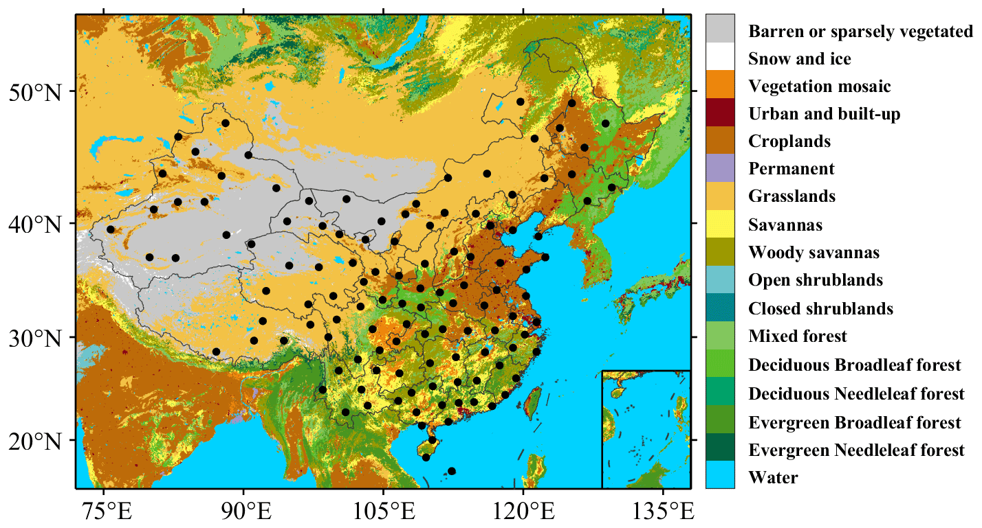
Figure 1 Geographical distribution of the radiosonde stations in China, which is overlaid over the surface land cover type distribution from MODIS observations. The color bar indicates the different surface land cover types.

Currently, there are multiple methods for observing wind profiles. Atmospheric reanalysis data such as the fifth-generation ECMWF reanalysis (ERA5), which is based on known physical mechanisms combined with the assimilation of a vast amount of observational data, have been widely used to derive the spatiotemporal distribution of wind profiles (Laurila et al., 2021; Gualtieri, 2021). The spaceborne Atmospheric Laser Doppler Instrument on board the Aeolus mission can only provide line-of-sight wind profile data, which can be further assimilated into atmospheric models to generate global wind profile products (Stoffelen et al., 2006; Guo et al., 2021). Nevertheless, the accuracy of wind profile products from Aeolus and ERA5 within the planetary boundary layer (PBL) requires improvement due to factors such as atmospheric attenuation and turbulence (Straume et al., 2020; Deng et al., 2022). On the other hand, ground-based wind measurements from towers or radar wind or lidar wind profilers can yield a highly precise wind profile for the PBL at the observation station (Durisic et al., 2012; Wu et al., 2022). However, single-site observations cannot provide wind profile data on a regional or national scale. Therefore, researchers are endeavoring to develop a theoretical model for wind profiles to acquire large-scale PBL wind profiles.

The wind profile model was initially developed based on the famous Monin–Obukhov similarity theory, which describes the wind profile using functions that rely on the stability parameter $h/L$ (Obukhov, 1946; Monin and Obukhov, 1954). The h stands for height, while L stands for the Obukhov length on the surface. The wind profile model based on similarity theory can be expressed in different forms depending on the atmospheric conditions. For neutral conditions, the wind speed profile model can be simplified to a logarithmic law (Powell et al., 2003; Marusic et al., 2013). For unstable conditions, an exponential better describes the wind speed profile in the surface layer over homogeneous terrain (Barthelmie et al., 2020). In engineering applications, most studies utilize a power-law model for the wind profile in the surface layer (Sen et al., 2012; Jung et al., 2021). This can achieve the conversion of the surface wind speed to the wind speed at wind turbine hub height. These wind profile models based on the Monin–Obukhov similarity theory have demonstrated effectiveness within the Prandtl layer and the surface layer. The Prandtl layer encompasses the initial tens of meters within the atmospheric boundary layer (Anderson, 2005). The top of the surface layer is approximately 100 m above the ground (Veers et al., 2019). Nevertheless, due to factors such as the Coriolis parameter, baroclinicity, and wind shear, the applicability of the Monin–Obukhov similarity theory breaks down above the surface layer (Optis et al., 2016; Tong et al., 2020). Therefore, extending wind profiles above the surface layer is of significance when applying wind profiles to wind energy assessment and PBL dynamics.

Above the surface layer, the wind profiles are influenced not only by the surface roughness, friction velocity, and atmospheric stability but also by factors including low-level jets, entrainment processes, and the Coriolis parameter (Gryning et al., 2007; Coleman et al., 2021). To obtain accurate wind profiles above the surface layer, some studies seek to introduce auxiliary variables to account for the influence of these factors. Gryning et al. (2007) established a straightforward model that regulates the combined length scale of wind profiles along with their stability correlations. This model is used to calculate wind profiles above the surface. On the other hand, Liu et al. (2022) present an analytical approach based on the Ekman equations and the foundation of the universal potential temperature flux profile. This approach enables one to describe the profiles of the wind and the turbulent shear stress, which in turn can capture aspects such as the wind veer profile. In addition, some studies have used machine learning (ML) technology to transform the surface wind speed and meteorological parameters to wind speeds at different heights. Yu et al. (2022) have devised a transfer method that leverages three ML methods, including the least absolute shrinkage selector operator, random forest (RF), and extreme gradient boost, for calculating the wind speed at 100 m. Liu et al. (2023) employed the RF model to estimate the wind speed at 120, 160 and 200 m. Nevertheless, the calculation procedure used by ML algorithms remains an unexplained process that does not clarify the input parameter's physical significance. Therefore, it is worth trying to combine ML algorithms with physical models to achieve the inversion of wind profiles above the surface layer.

The present study aims to extend wind profiles beyond the surface layer by combining physics and machine learning approaches. For this purpose, we attempt to combine the power-law method (PLM) with the RF, resulting in a model named PLM-RF, to extend wind profiles beyond the surface layer. The PLM-RF model is trained and tested using radiosonde (RS) data and reanalysis gridded meteorological data over China. A performance comparison of the PLM, RF, and PLM-RF models is also carried out. Then, the wind profile generated by the PLM-RF model is evaluated against RS observations, which is followed by an independent validation of the model at Atmospheric Radiation Measurement (ARM) sites. The results of our study have great implications for the weather, climate, and renewable energy sector.

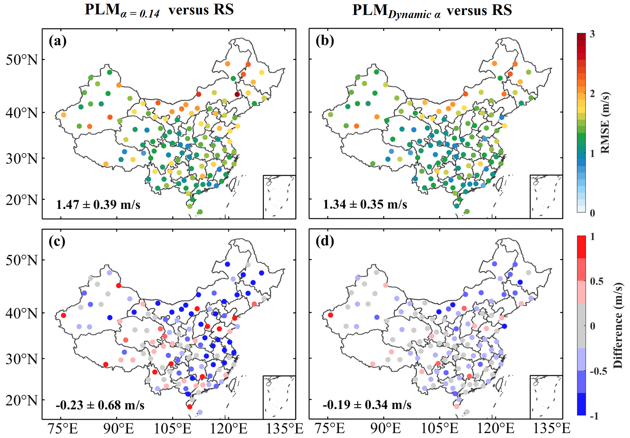
Figure 2 The spatial distributions of (a, b) the RMSE and (c, d) the difference for the WS₁₀₀ estimated by the traditional PLM (constant α of 0.14) and PLM (dynamic α). Also shown in the bottom left corner of each map are the mean values of the RMSE and the difference.

2 Materials and data

2.1 Land cover type data

The land cover type data are derived from the Moderate Resolution Imaging Spectroradiometer (MODIS), a satellite-borne instrument that captures images and measures a wide range of surface properties such as the land surface temperature, vegetation cover, and atmospheric aerosols (Friedl et al., 2002). The high spatial resolution of the instrument enables the identification of diverse land features, including forests, urban areas, and agricultural fields, thereby making it an important instrument for the purpose of environmental monitoring and land management (Sulla-Menashe et al., 2018). MODIS provides two land cover type products: MCD12Q1 and MCD12C1. MCD12Q1 comprises observation data from different regions, which require self-splicing. MCD12C1 comprises annual concatenated data (one image per year). Following the previous study (Liu et al., 2020), the land cover type data used here were obtained from MCD12C1 and are named “MCD12C1.A2021001.061.2022217040006”. Figure 1 displays the geographic distribution of the dominant land cover types in China. The land cover type data help us to determine the power-law exponent (α).

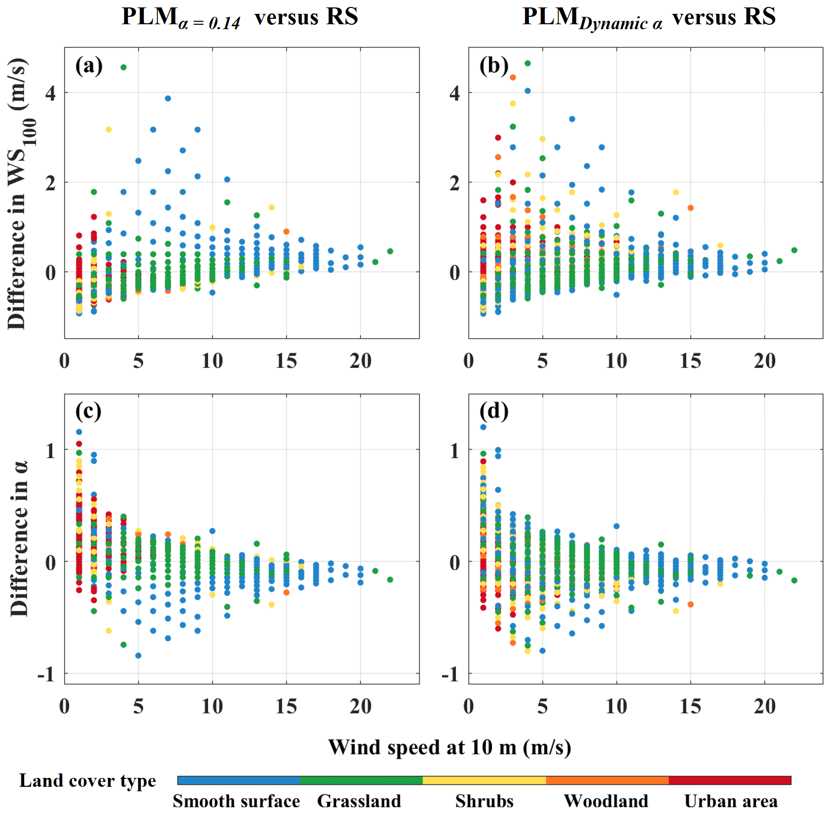
Figure 3 The differences in (a, b) WS₁₀₀ and (c, d) α estimated by PLM (α=0.14) and PLM (dynamic α) relative to RS observations shown as a function of land cover type (color shading). The color bar indicates the various land cover types.

2.2 Radiosonde measurements

An L-band RS can measure profiles of the atmospheric temperature, pressure, humidity, wind direction, and wind speed in situ. Measurements are taken at 1 min intervals starting from the ground surface up to approximately 30 km a.g.l. (above ground level) (Guo et al., 2016). RS observations are conducted at 119 observation stations in China, which are shown in Fig. 1. RSs are launched twice per day at around 08:00 and 20:00 local time (LT). Here, the wind speed profiles from RS measurements at 119 stations are used as reference values (National Meteorological Science Data Center, 2023). The RS observations were made between 1 June 2020 and 30 May 2021. In addition, the drift of the RS during its ascent was investigated, as illustrated in Fig. S1 in the Supplement. The coordinates of the RS and observation station within a height of 0.5 km indicated that the drifting distance was less than 0.5 km. This indicates that the drift of the RS will not impact the attainment of wind profiles in the surface layer.

2.3 ERA5 data

ERA5 is a fifth-generation reanalysis dataset that offers a range of atmospheric parameters, such as temperature, humidity, pressure, and radiation (Hersbach et al., 2020). Following a previous study (Liu et al., 2023), nine surface parameters are obtained in this study, including the Charnock coefficient (Char), forecast surface roughness (FSR), friction velocity (FV), dew point (DP), temperature (Temp), pressure (Pres), net solar radiation (Rn), latent heat flux (LHF), and sensible heat flux (SHF). These parameters are processed into grid data with a 0.25°×0.25°size and an hourly time resolution. Based on the longitude and latitude information for the RS and ARM stations, those parameters in the corresponding grid are obtained accordingly. These data are also collected for the period from 1 June 2020 to 30 May 2021.

2.4 ARM data

The ARM user facility was established by the US Department of Energy (Lubin et al., 2020; Zhang et al., 2022). It sets up observation stations and instruments for atmospheric observation experiments globally, making the atmospheric observations, including temperature, wind, radiation, and cloud properties, publicly accessible (Liu et al., 2022). Wind profile data from the Doppler wind lidars deployed at the eastern North Atlantic (ENA), North Slope of Alaska (NSA), and Southern Great Plains (SGP) stations are collected for independent comparison with the proposed method. Statistical parameters such as the coefficient of determination (R²), mean absolute error (MAE), and root mean squared error (RMSE) are used to quantify the comparison results. Figure S2 presents the geographic locations and land cover types of the three lidar stations. ENA is situated on an Atlantic Ocean island with ocean as its primary land cover, NSA is situated on Alaska's north coast with grassland as its ground cover, and SGP is located in the Great Plains in the central United States where grassland is also the dominant land cover. The Doppler wind lidar observations cover the period from 1 June 2020 to 30 May 2021. Moreover, these wind profiling measurements are processed as hourly averages so that they correspond with other data.

3 Methods

3.1 Power-law method

The PLM assumes that wind speed increases exponentially with height (Hellman et al., 1914). The wind profile can be calculated based on the surface wind speed (v₀) using the following formula:

$$\begin{array}{}\text{(1)}& v_i=v_{\mathrm{0}}\times {\left({\displaystyle \frac{h_i}{h_{\mathrm{0}}}}\right)}^{\mathit{\alpha }},\end{array}$$

where v_i represents the wind speed at height h_i. h₀ is the measurement height of v₀. Here, v₀ is observed by an anemometer at a height of 10 m above the ground. α is the power-law exponent, which varies with land cover type, height, and time (Li et al., 2018).

α is usually set as a constant (0.14) for the purpose of approximating the wind profile at stations with no available observations or empirical formulas. Figure 2a and c show the RMSE and difference between the PLM (α=0.14) results and the RS measurements of the wind speed at 100 m (WS₁₀₀). The average RMSE and difference over China are 1.49±0.39 and $-\mathrm{0.23}\pm \mathrm{0.68}$ m s⁻¹, respectively. The results indicate that PLM (α=0.14) underestimates the wind profile at almost a quarter of the sites (Fig. 2c). These results suggest that the estimation of wind profiles based on a constant α value is subject to large errors. Some studies have also confirmed this (Jung et al., 2021; Liu et al., 2023). Furthermore, other studies have demonstrated that the value of α differs with the land cover type due to varying surface roughness (Durisic et al., 2012). An empirical lookup table is summarized with respect to the setting of α, as shown in Table S1 in the Supplement. The value of α ranges from 0.1 to 0.4 with increasing surface roughness. Based on the MODIS land cover type dataset, the corresponding value of α can be obtained for each RS site. Figure 2b and d show the RMSE and the difference between the PLM (dynamic α) results and the RS measurements. Compared with the PLM (α=0.14) results, the results of PLM (dynamic α) are improved. However, the results of PLM (dynamic α) are still underestimates for most stations in the northeastern and Inner Mongolia regions.

3.2 Random forest model

The RF model is a nonlinear fitting algorithm that has been used to calculate wind profiles (Yu et al., 2022; Liu et al., 2023). Here, the RF model is also used to fit the surface parameters to obtain the wind profile. The input variables include surface wind speed (WS), surface wind direction (WD), land cover type (Type), altitude (Alt), longitude (Lon), latitude (Lat), month (M), hour (H), Char, FSR, FV, DP, Temp, Pres, Rn, LHF, and SHF. The reference value is the wind speed provided by RS. In addition, the parameter tuning of the RF model directly affects the performance and generalization ability of the model (Zhu et al., 2021). The parameter tuning process for estimator number and minimum leaf size is shown in Fig. S3. The minimum RMSE (1.02 m s⁻¹) and maximum R (0.91) are obtained when Estimator number is 300 and Min Leafsize is 5. Therefore, the Estimator number and the Min Leafsize are set to 300 and 5 for the RF model, respectively.

3.3 Combining the physical and RF models

In this study, we propose a novel method, termed PLM-RF, that combines the PLM and the RF model to estimate wind profiles. Its principle is to treat the wind profile as a power-law distribution in the vertical direction, with α fitted by using the RF model. Further details about this method are given below.

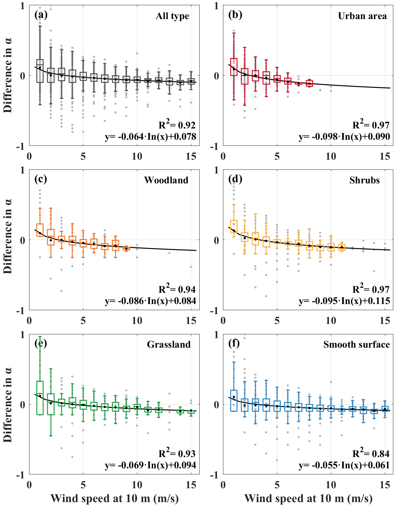
Figure 4 The α bias (assumed value minus observed value) at 100 m as a function of the surface wind speed over (a) all types of land cover, (b) urban areas, (c) woodland, (d) shrubs, (e) grassland, and (f) smooth surfaces.

3.3.1 Physical constraint

Previous studies have confirmed that the wind profile in the surface layer adheres to a power-law distribution (Liu et al., 2023). The primary reason for the error is the uncertainty in the value of α. Therefore, to achieve more accurate results, it is necessary to first analyze the reasons for the error. Figure 3a–b show the differences in WS₁₀₀ estimated by PLM (α=0.14) and PLM (dynamic α) relative to RS observations. Based on MODIS land cover type data, each of the 119 RS sites is classified as either an urban area, woodland, shrubs, grassland, or a smooth surface. It is found that, regardless of the land cover type, the difference in wind speed decreases as the surface wind speed increases. Similarly, the difference between the assumed α and the observed α at 100 m decreases with increasing surface wind speed (Fig. 3c–d). These results indicate that there is a relationship between the error of the PLM results and the surface wind speed. This may be due to the limited influence of surface friction on the wind profile. When the wind speed within the PBL is low, factors such as surface friction and the Coriolis force complicate the vertical distribution of the wind profiles, leading to a low surface wind speed and large errors in the PLM (Wang et al., 2023). On the contrary, when the wind speed within the PBL is high, the effect of surface friction can be neglected to some extent. This results in the real wind profile being closer to the power-law distribution, thereby reducing the error of the PLM results.

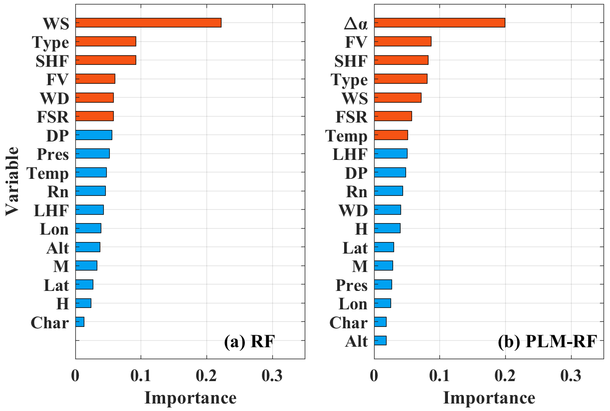
Figure 5 The importance scores of predictor variables for the (a) RF and (b) PLM-RF models. WS: surface wind speed; WD: surface wind direction; Type: land cover type; Alt: altitude; Lon: longitude; Lat: latitude; M: month; H: hour; Char: Charnock coefficient; FSR: forecast surface roughness; FV: friction velocity; DP: dew point; Temp: temperature; Pres: pressure; Rn: net solar radiation; LHF: latent heat flux; SHF: sensible heat flux; and Δα: correction factor for α.

To quantify the effect of the surface wind speed on α, the α bias (assumed value minus observed value) at 100 m is examined as a function of surface wind speed over different land cover types, as shown in Fig. 4. The gray dots and black lines indicate the sample points and the logarithmic curve, respectively. The coefficients of determination between the surface wind speed and the difference in α on all land cover types, an urban area, woodland, shrubs, grassland, and a smooth surface are 0.92, 0.97, 0.94, 0.97, 0.93, and 0.84, respectively. These indicate that there is a good correlation between the surface wind speed and difference in α. Therefore, the correction factor for α (Δα) can be defined statistically based on the land cover type and surface wind speed. The correction functions for α for different land cover types are also plotted in Fig. 4. For each sample, Δα can be calculated by the correction functions and can then be used in the fitting of the RF model as a physical constraint to improve the accuracy. In addition, the α bias as a function of surface wind speed at different heights is also investigated, as shown in Fig. S4. At 50, 100, 150, 200, 250, and 300 m, the coefficients of determination between the surface wind speed and the difference in α are larger than 0.9. This indicates that Δα can be constructed using the surface wind speed to improve the accuracy of the inversion of wind speed at high altitude.

3.3.2 Model construction

For the PLM-RF model, the wind profile is considered to have a power-law distribution, and α is fitted by the RF model. The inputs include Δα, WS, WD, Type, Alt, Lon, Lat, M, H, Char, FSR, FV, DP, Temp, Pres, Rn, LHF, and SHF. The reference value is the α calculated from RS observations. The tuning parameter evolution for the PLM-RF model is shown in Fig. S5. The RMSE reaches a minimum (0.91 m s⁻¹) and R reaches a maximum (0.93) when Estimator number is 500 and Min Leafsize is 5. Therefore, Estimator number and Min Leafsize are set to 500 and 5, respectively.

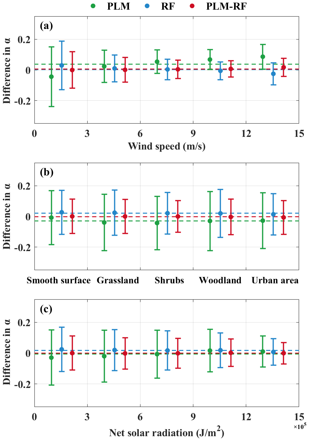
Figure 6 The mean and standard deviation of the difference between the assumed α and the observed α at 100 m as a function of (a) surface wind speed, (b) land cover type, and (c) net solar radiation. Green, blue, and red lines represent the results from PLM, RF, and PLM-RF, respectively.

To comprehend the model's physical meaning, an importance analysis of the inputs is performed for the RF and PLM-RF models, as shown in Fig. 5. The relevant features that can affect the accuracy of the model accuracy are marked with red bars. For the RF model, the relevant features are WS, Type, SHF, FV, WD, and FSR. The importance of WS, Type, and SHF is greater than the importance of the other features. WS is the surface wind speed. Type is the value of α based on the land cover type. From the perspective of a physical meaning, the RF model calculates wind profiles through complex fitting methods based on the surface wind speed and meteorological conditions. In contrast, for the PLM-RF model, Δα, FV, SHF, Type, WS, FSR, and Temp are the relevant features. Δα is the most important, but Type and WS are ranked fourth and fifth in importance, respectively. In addition, the importance of FV ranks second. FV is used to calculate the way that the wind changes with height at the lowest levels of the atmosphere (Liu et al., 2023). These results indicate that the PLM-RF model calculates the way that the wind speed changes in the vertical direction. In addition, SHF and FSR are both relevant features in the construction of the RF and PLM-RF models. This indicates that surface roughness and solar radiation are factors that need to be considered in the calculation of wind profiles.

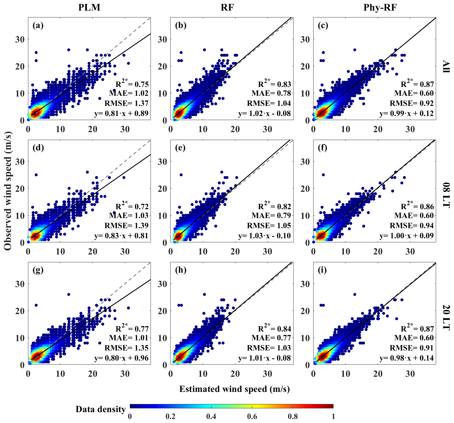
Figure 7 Comparisons between the observed WS₁₀₀ and the estimated WS₁₀₀ for the (a, d, g) PLM, (b, e, h) RF, and (c, f, i) PLM-RF models for all times at 08:00 and at 20:00 LT. The gray and black lines are the reference and regression lines, respectively. The color bar represents the data density. The asterisk indicates that the correlation coefficient (R) passed the t test at a confidence level of 95 %.

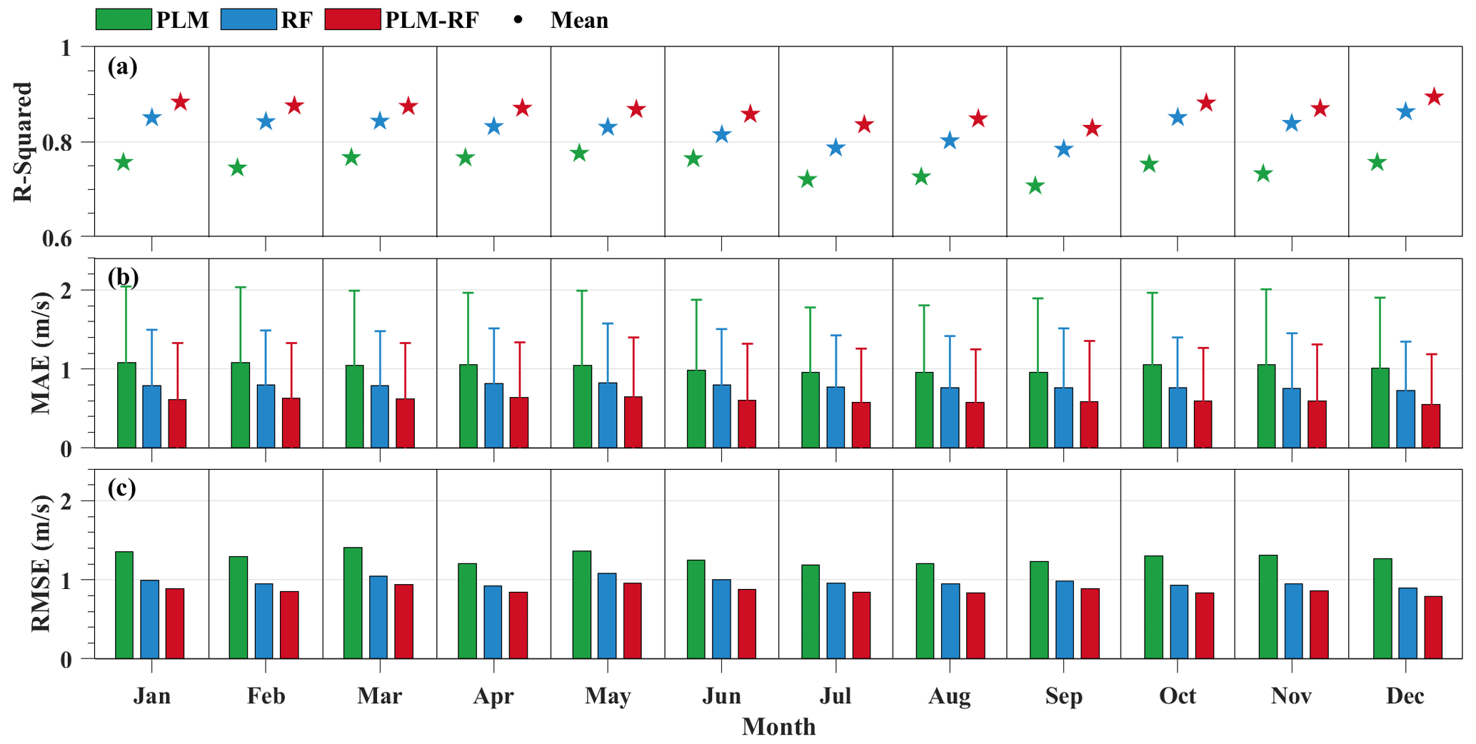
Figure 8 Annual cycles of the (a) R², (b) MAE, and (c) RMSE between the estimated WS₁₀₀ and the observed WS₁₀₀ for the PLM, RF, and PLM-RF models. The green, blue, and red colors represent the PLM, RF, and PLM-RF methods, respectively.

3.4 Sensitivity analysis

The average value and standard deviation of the difference between the assumed α and the observed α are illustrated for the primary input features in Fig. 6. Green, blue, and red represent the PLM, RF, and PLM-RF models, respectively. The differences in deviations for PLM-RF models decrease slightly with increasing surface wind speed. Moreover, the mean and deviation of the difference for the PLM-RF model are relatively stable and do not vary with the land cover type. These results indicate that both the RF and PLM-RF models exhibit good generalization across different land cover types and surface wind speeds. This is due to the fact that the RF model considers random perturbations in the sample space to improve generalization ability (Breiman, 2001). In addition, due to the samples only being obtained at 08:00 and 20:00 LT, it is noted whether or not the performance of the PLM-RF model is affected by time. The RS observation stations are geographically distributed in several time zones, but they are all observed at the same time. This means that although the recording time of the RS measurements is 08:00 or 20:00 LT, the training and test samples contain observation data from multiple time periods. Therefore, Rn is used as a measure of time to investigate the applicability of the methods (Fig. 6c). For the three methods, the mean of the difference is relatively stable and the standard deviation of the difference decreases slightly as Rn increases. This indicates that the generalization of the PLM-RF model within the sample is reliable. However, the Rn in China at noon can reach 1.5–2×10⁶ J m⁻², which exceeds the upper limit of the input values in the current sample. This indicates that the generalization of the PLM-RF model at noon cannot be proven based on the existing training and test samples. Therefore, we must rely on the Doppler wind lidar observations from the ARM sites for comparison to evaluate the performance of the PLM-RF model at noon. Specific comparisons will be discussed in Sect. 4.4.

4 Results and discussion

In this section, the performances of the PLM, RF, and PLM-RF models are first compared by conducting intercomparison analyses. The wind profiles calculated by the PLM-RF model are then evaluated by comparing them with the RS observations. Finally, the PLM-RF model is applied to three ARM sites for independent validation.

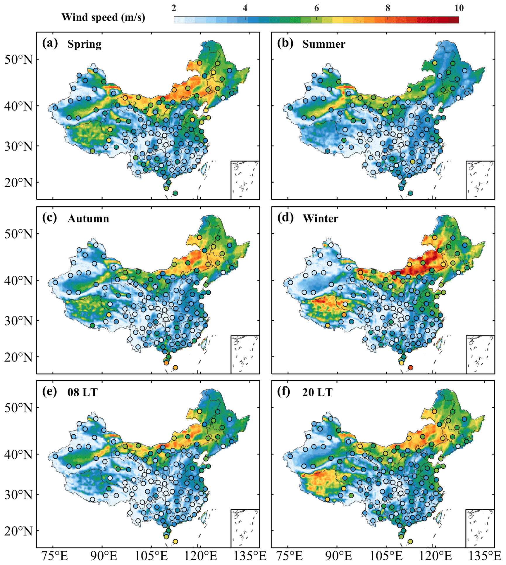
Figure 9 Spatial distributions of the mean WS₁₀₀ from ERA5 (colored shading) and the PLM-RF model (colored dots) in (a) spring, (b) summer, (c) autumn, and (d) winter as well as at (e) 08:00 LT and (f) 20:00 LT.

4.1 Intercomparison of different methods

Figure 7 displays scatter plots of the estimated WS₁₀₀ versus the observed WS₁₀₀ for all three methods at different times. Overall, the R² (RMSE) of the WS₁₀₀ from the PLM, RF, and PLM-RF at all times is 0.75 (1.37 m s⁻¹), 0.83 (1.04 m s⁻¹), and 0.87 (0.92 m s⁻¹), respectively. The accuracy of the RF and PLM-RF models is better than that of the PLM. For the PLM, most of the estimated WS₁₀₀ values are underestimated when the observed wind speed is high. This is because the PLM relies on an exponential relationship to calculate the WS₁₀₀. However, the wind profile is affected by turbulence, surface friction, and other factors (Tieleman, 1992; Solanki et al., 2022). The exponential law based on constants is unable to obtain the WS₁₀₀ with high accuracy. In contrast, the RF and PLM-RF models show significantly improved performance. The RF and PLM-RF models consider more environmental factors, such as SHF and FV, in the inversion process. They improve the accuracy of the model because the effects of surface friction and surface radiation flux on the wind profiles are taken into account. Briefly, these two methods rely on a dynamic α to invert the wind profiles. Each site uses an α that varies with environmental factors, resulting in improved accuracy of inversion. In particular, for the PLM-RF model, the correction function for α can be used to obtain a value of α that is closer to the observed α, resulting in the highest R² (0.87) and the lowest MAE (0.60 m s⁻¹). In addition, the MAE values of the WS₁₀₀ from the PLM, RF, and PLM-RF at 08:00 (20:00) LT are 1.03 (1.01), 0.79 (0.77), and 0.60 (0.60) m s⁻¹, respectively. Comparisons of the results for both 08:00 and 20:00 LT also show that the performance of PLM-RF is the best, followed by RF and finally by PLM.

Figure 8 shows the R², MAE, and RMSE between the estimated WS₁₀₀ and the observed WS₁₀₀ for the three methods in different months. The R² is relatively consistent between months, irrespective of the method used (Fig. 8a). For the PLM, the monthly mean MAE values are higher during the cold season (October–April) than during the warm season (June–September). This is because the wind speed variations are more complex during the cold season. Large-scale synoptic systems have a relatively high frequency of occurrence during the cold season (Liu et al., 2019). Compared with PLM, the RF and PLM-RF models show stable accuracy over the 12 months; i.e., the difference between the months is relatively small. The monthly mean MAE of the PLM-RF model does not show significant seasonal differences. This indicates that the PLM-RF model is not affected by seasonal variation, which is because the RF models are data-driven (Zhu et al., 2021; Ma et al., 2021). After correcting the α based on the RF model, the PLM-RF model can effectively overcome the influence of seasonal factors. Figure 8c shows that the WS₁₀₀ from the PLM-RF model has a smaller RMSE in each month, and the RMSE is relatively stable over the 12 months. The results indicate that the PLM-RF model outperforms both the PLM and RF in terms of accuracy and stability. Therefore, the PLM-RF model may be a more suitable choice for estimating wind profiles in China than either RF or PLM.

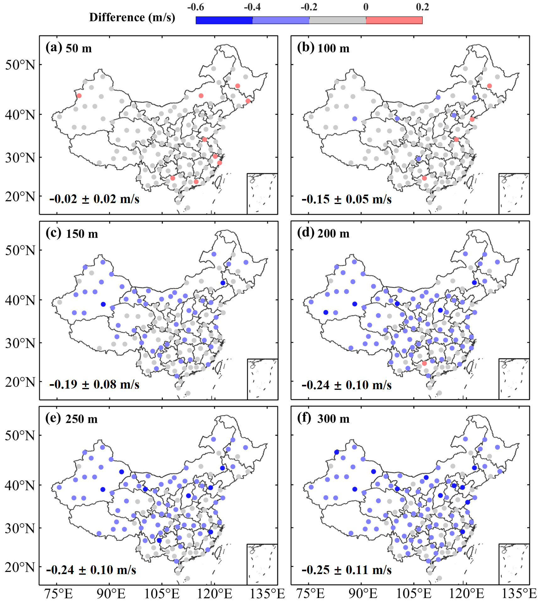
Figure 10 The spatial distribution of the difference between the estimated wind speed and the observed wind speed for the PLM-RF model over 120 radiosonde stations in China at different heights: (a) 50 m, (b) 100 m, (c) 150 m, (d) 200 m, (e) 250 m, (f) 300 m.

4.2 Wind speed evaluation of the PLM-RF model

Figure 9 shows the spatial distributions of the mean wind speed from ERA5 (colored shading) and the PLM-RF model (colored dots) at 100 m for different periods. In general, the mean WS₁₀₀ values of ERA5 and the PLM-RF model are similar. Regarding the seasonal variation, the WS₁₀₀ is low in summer and fall and high in spring and winter. This is due to large-scale synoptic systems that occur often in the cold season (Liu et al., 2019). Regarding the spatial distribution, the WS₁₀₀ is highest in Inner Mongolia and northeastern China, followed by coastal areas, and it is lowest in inland areas. There are two reasons for the high wind speeds in Inner Mongolia and northeastern China. One is that the climate in these areas is dry and cold, especially in winter. The low temperature and high air density lead to the formation of a strong pressure gradient (Liu et al., 2019). When the pressure gradient is large, cyclonic and anticyclonic weather will occur, resulting in higher wind speeds. Another reason is that these areas are susceptible to the influence of the Siberian monsoon and warm currents from the Pacific (Yu et al., 2016). This monsoon causes an increase in wind speed as it passes through Inner Mongolia and northeastern China. In addition, comparisons between the WS₁₀₀ from ERA5 and that from the PLM-RF model for different periods are shown in Fig. S6. Although the output of the PLM-RF model has a good correlation with the WS₁₀₀ from ERA5, there are still some differences. Most of the WS₁₀₀ values from the PLM-RF model are greater than those from ERA5 when the wind speed is high. This is because Δα is introduced in the PLM-RF model, which makes the model tend to produce large output values.

Figure 10 shows the spatial distribution of the difference between the estimated wind speed from the PLM-RF model and the RS observation at different heights. At 50 and 100 m, most sites (more than 90 %) show a mean difference of less than 0.2 m s⁻¹, with an overall mean difference of $-\mathrm{0.02}\pm \mathrm{0.02}$ and $-\mathrm{0.15}\pm \mathrm{0.05}$ m s⁻¹, respectively. In contrast, above 100 m, the average differences are negative at almost all sites. The mean differences for all sites at 150, 200, 250, and 300 m are $-\mathrm{0.19}\pm \mathrm{0.08}$, $-\mathrm{0.24}\pm \mathrm{0.10}$, $-\mathrm{0.24}\pm \mathrm{0.10}$, and $-\mathrm{0.25}\pm \mathrm{0.11}$ m s⁻¹, respectively. Compared to the results of the PLM (Fig. 2c and d), the accuracy of the wind speed in the PLM-RF model is improved. Overall, the wind speed estimated by the PLM-RF model is slightly underestimated compared to the observed value. Moreover, the average difference gradually increases with increasing height. This is because the wind profile above the surface layer is not logarithmic; it increases faster in response to the reduction in surface friction force (Gryning et al., 2007; Liu et al., 2023). The RMSE and MAE between the estimated and observed wind speeds at different heights can be seen in Figs. S7 and S8. These results also confirm that the performance of the PLM-RF model decreases with increasing height. This is because the wind profile above the surface layer is affected by the influence of low-level jets, entrainment processes, and the Coriolis parameter (Coleman et al., 2021). In addition, the spatial distributions of RMSE and MAE indicate that the performance of the PLM-RF model may be influenced by the terrain.

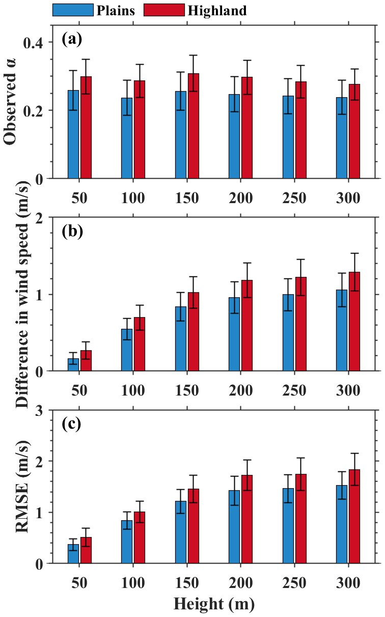
Figure 11 (a) The mean α observed by RS as a function of height. (b) The difference and (c) the RMSE between the estimated wind speed and the observed wind speed as a function of height. Blue and red boxes represent the results over plains and highland areas, respectively.

4.3 Effect of terrain

To evaluate the effect of the terrain factor on the performance of the PLM-RF model, the plain terrain is defined as the terrain in which the topographic relief is less than 50 m within a radius of 5 km around the observation station. The RS sites are divided into two categories: plains (marked by red dots in Fig. S9) and highlands (marked by black dots in Fig. S9). Figure 11a shows the mean α observed by RS at different heights. Blue and red boxes represent the results over plains and highland areas, respectively. The mean α in highlands is greater than that in plains. This indicates that the variation of wind profiles in highlands is more complex than that in plains. Previous studies have also shown that valley winds and low-level jets can complicate the wind profiles in the PBL (Solanki et al., 2021; Wang et al., 2023). Figure 11b shows the difference between the estimated and observed wind speeds for the PLM-RF model at different heights. The difference in highlands is obviously larger than that in plains. Moreover, similar phenomena were also found in the results for the RMSE (Fig. 11c). The RMSE in highlands is relatively large, while it is relatively small in plains. This may be due to differences in terrain. The terrain in plains is mainly flat, while the terrain in highlands is mainly mountainous (Chen et al., 2016). The wind profile is not only affected by factors such as surface friction and solar radiation, but it is also constrained by the terrain (Panofsky et al., 1964; Jung et al., 2021). In the construction of the PLM-RF model, the influence of the terrain factor was not considered, resulting in a higher RMSE of the PLM-RF model in the highlands.

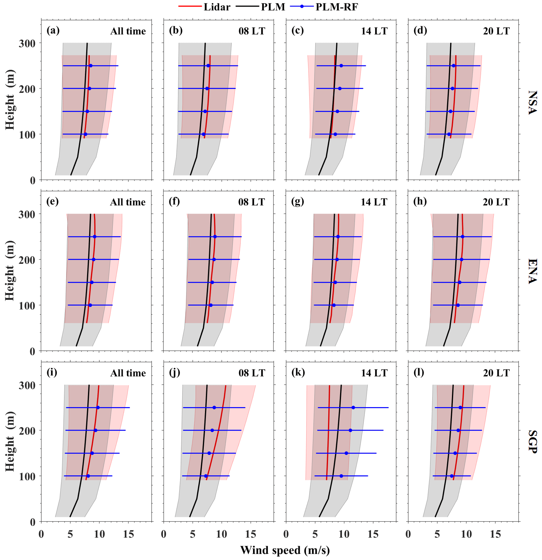
Figure 12 Vertical profiles of the wind speed from different methods at three ARM sites: (a–d) NSA, (e–h) ENA, and (i–l) SGP. Red, black, and blue lines represent mean wind profiles from Doppler wind lidar, PLM, and PLM-RF, respectively, and their corresponding color-shaded areas represent the standard deviation.

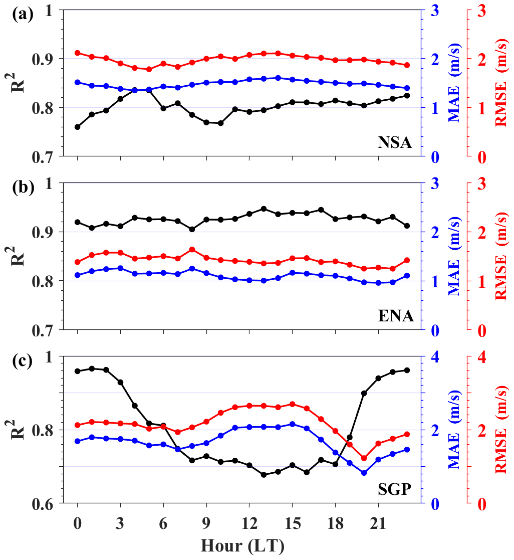
Figure 13 Diurnal variations of the R² (black lines), MAE (blue lines), and RMSE (red lines) between the WS₁₀₀ calculated by the PLM-RF model and the WS₁₀₀ observed by Doppler wind lidars at the (a) NSA, (b) ENA, and (c) SGP sites.

4.4 Independent validation

Figure 12 displays the vertical wind speed distribution estimated using different methods at three ARM sites. At the NSA site, the wind profiles calculated by the PLM-RF model are similar to the observed values at 08:00 and 20:00 LT, but they are slightly overestimated at 14:00 LT. The performance of the PLM-RF model at 14:00 LT is inferior to that of the PLM (Fig. 12c). This phenomenon also occurs at the SGP site. The results of the PLM-RF model are significantly overestimated at 14:00 LT. These results indicate that the performance of the PLM-RF model is influenced by hourly variations. However, to our surprise, the result of the PLM-RF model is very consistent with the observations at the ENA site, even at 14:00 LT (Fig. 12g). This may be due to the differences in land cover type between the sites. Although the PLM-RF model produces some overestimation at 14:00 LT, the comparisons made at other times indicate that the wind profiles of the PLM-RF model are still like the observed results (Fig. 12a, e and i). The PLM-RF model's wind profiles exhibit greater proximity to the observed values when compared to the results generated by the PLM at the three ARM sites.

To further evaluate the performance of the PLM-RF model, the diurnal variations of the R², MAE, and RMSE between the WS₁₀₀ calculated by the PLM-RF model and the WS₁₀₀ observed by Doppler wind lidar are shown in Fig. 13. At the SGP site, the R² is higher in the nighttime and lower in the daytime. These results confirm that the performance of the PLM-RF model at the SGP site is influenced by diurnal variations. This is because the generalization of the RF algorithm depends on the training and test samples (Zhu et al., 2021). As mentioned in Sect. 3.4, the training and test samples of the PLM-RF model do not actually contain any in situ measurements from the period 11:00 to 15:00 LT. This means that the PLM-RF model has no generalization at noon, resulting in poor accuracy of the PLM-RF model during the daytime. On the contrary, the performance of the PLM-RF model is stable at the NSA and ENA sites. This is because the SGP site is located over land and therefore experiences significant diurnal variations in wind speed. The wind speed in the daytime is relatively low – even lower than the estimated value from the PLM. In contrast, the ENA site is located on an island, so the diurnal variation of wind speed is not significant. The wind speed throughout the day is higher than the estimated value from the PLM. For the PLM-RF model, since the training data are mainly composed of relatively high wind speeds in the nighttime, the model exhibits a significant overestimation correction. The model can accurately calculate the wind speed when the actual value is larger than the estimated value from the PLM, while it will significantly overestimate the actual value if it is lower than the estimated value from the PLM. Overall, the wind speed results retrieved by the PLM-RF model are consistent with the Doppler wind lidar measurements at different heights. These results indicate that the PLM-RF model has good spatial applicability and can be used to obtain the wind profiles on different land cover types.

5 Summary and conclusions

The traditional wind profile model was constructed based on the Monin–Obukhov similarity theory. As a result, the wind profile based on the similarity theory is only effective within the surface layer. To address this challenge, this study proposed a PLM-RF method that combines the traditional PLM with the RF algorithm to extend wind profiles beyond the surface layer.

The reasons for the errors in the PLM above the surface layer were first analyzed. The result indicated that the error in the PLM is mainly attributable to the α setting. This is because the wind profile above the surface is affected by factors such as the surface roughness, friction velocity, low-level jets, and the Coriolis parameter, causing α to have complexity. Moreover, the surface wind speed has a certain impact on the variation of α. At heights of 50, 100, 150, 200, 250, and 300 m, the coefficients of determination between the surface wind speed and the difference in α are greater than 0.9. This may be due to the limited influence of surface friction on the wind profile. When the PBL wind is high, the effect of surface friction can be neglected to some extent, resulting in the real wind profile being closer to the power-law distribution. Based on this physical constraint, the PLM-RF method considers the wind profile to have a power-law distribution in the vertical direction, and the α values at different heights are fitted by the RF model to calculate the wind profile. A performance comparison of the PLM, RF, and PLM-RF methods was then carried out based on the RS observations made over China from 1 June 2020 to 30 May 2021. The R² (MAE) values of the WS₁₀₀ from the PLM, RF, and PLM-RF models were 0.75 (1.02 m s⁻¹), 0.83 (0.78 m s⁻¹), and 0.87 (0.60 m s⁻¹), respectively. This shows that the PLM-RF model has better accuracy and stability compared to the PLM and RF. Especially for high-wind-speed events, the output of PLM is significantly low, while the PLM-RF model can effectively correct this underestimation. The PLM-RF model can be understood as the PLM based on a dynamic α. The RF model is used to adjust α at different heights based on factors such as surface wind speed, land cover type, and meteorological parameters to achieve high-precision wind profile inversion.

Overall, the advantage of the PLM-RF model is that it can provide more accurate wind profiles than the PLM, especially when the actual wind speed is high. Moreover, the PLM-RF model is not affected by seasonal variation. This is because the RF model is data-driven. The training sample of the PLM-RF model contains enough samples from the four seasons. The PLM-RF model is recommended for areas with high wind speeds, such as coastal areas. The limitation of the PLM-RF model is that its performance is affected by the diurnal variation and terrain. The generalization of the RF model depends on whether the training samples contain sufficient sample inputs. The training samples of the PLM-RF model do not contain in situ measurements from the time period of 11:00 to 15:00 LT, resulting in relatively poor accuracy during this period. Similarly, the RMSE of the wind profiles is relatively large in highland areas, which is likely due to the fact that the influence of the terrain was not considered in the construction of the PLM-RF model. Therefore, it is not recommended to use the PLM-RF model for the period from 11:00 to 15:00 LT over highland areas before including observation data to constrain the model.

Our study extends the wind profile beyond the surface layer by combining physical and ML approaches, which has great implications for the weather, climate, and renewable energy sector. However, due to limitations in data size and terrain factors, the performance of the PLM-RF model above water surfaces is uncertain. In the future, global RS observation data will be used to train and test the PLM-RF model and evaluate its performance on a global scale.