the Creative Commons Attribution 4.0 License.
the Creative Commons Attribution 4.0 License.
 | 03 Apr 2024
Negligible temperature dependence of the ozone–iodide reaction and implications for oceanic emissions of iodine
Ryan J. Pound
Lyndsay S. Ives
Matthew R. Jones
Stephen J. Andrews
Lucy J. Carpenter
The reaction between ozone and iodide is one of the main drivers of tropospheric ozone deposition to the ocean due to the ubiquitous presence of iodide in the ocean surface and its rapid reaction with ozone. Despite the importance of this sea surface reaction for tropospheric ozone deposition and also as the major source of atmospheric iodine, there is uncertainty in its rate and dependence on aqueous-phase temperature. In this work, the kinetics of the heterogeneous second-order reaction between ozone and iodide are investigated using conditions applicable to coupled ocean–atmosphere systems (1 × 10⁻⁷–1 × 10⁻⁵ M iodide; 40 ppb ozone; 288–303 K; 15.0 psi). The determined Arrhenius parameters of A = 5.4 ± 23.0 × 10¹⁰ and Ea = 7.0 ± 10.5 kJ mol−1 show that the reaction has a negligible positive temperature dependence, which could be weakly negative within errors. This is in contrast to a previous study that found a strong positive activation energy and a pre-exponential factor many orders of magnitude greater than determined here. The re-measured kinetics of ozone and iodide were used to constrain a state-of-the-art sea surface microlayer (SML) model. The model replicated results from a previous laboratory study of the temperature dependence of hypoiodous acid (HOI) and molecular iodine (I2) emissions from an ozone-oxidised iodide solution. This work has significance for the global modelling of the dry deposition of ozone to the ocean and the subsequent emissions of iodine-containing species, thus improving the understanding of the feedback between natural halogens, air quality and climate change.
- Article
(2803 KB) - Full-text XML
- BibTeX
- EndNote


Ozone (O3) is an important tropospheric pollutant and greenhouse gas, with estimated radiative forcing of 0.40 W m−2 (reported ranges span 0.20–0.65 W m−2) (Watson et al., 1995; Ramaswamy et al., 2001; Forster et al., 2007; Myhre et al., 2013). Ozone concentrations must be monitored and accurately predicted, as short-term exposure can harm the respiratory and cardiovascular systems in humans, while long-term exposure is thought to contribute to respiratory mortality and new-onset asthma in children (Nuvolone, 2018). Tropospheric ozone also poses a risk to global food production due to its phytotoxic effects on crop plants, including the destruction of photosynthetic pigments and decrease in crop growth and productivity (Rai and Agrawal, 2012). The tropospheric ozone burden (∼ 340 Tg) is controlled by a balance of influx from the stratosphere (∼ 550 Tg (O3) yr−1), chemical production (∼ 5100 Tg (O3) yr−1), chemical destruction (∼ 4650 Tg (O3) yr−1) and dry deposition (∼ 1000 Tg (O3) yr−1) to the Earth's surface (Stevenson et al., 2006).
Oceanic dry deposition, though considerably slower than deposition to crops and soil (Wesely and Hicks, 2000), is influential in global atmospheric models due to the significant coverage of the Earth by oceans. The dry deposition of ozone to the ocean surface is estimated to contribute approximately a quarter of the total loss of ozone from the atmosphere and represents the single largest deposition flux of ozone (mean of 361 Tg (O3) yr−1 calculated from 15 different models) (Hardacre et al., 2015).
The dry deposition velocity (vd) of ozone to the ocean has been reported by several authors with highly variable results but typically of the order of 0.01–0.10 cm s−1 (Galbally and Roy, 1980; Garland et al., 1980; Wesely et al., 1981; Lenschow et al., 1982; Kawa and Pearson Jr., 1989; McKay et al., 1992; Heikies et al., 1996; Gallagher et al., 2001; Whitehead et al., 2009; McVeigh et al., 2010; Helmig et al., 2012). In lieu of accurate parameterisation methods, global ozone models typically apply a single global deposition velocity of 0.05 cm s−1 despite large variances in measured values (Ganzeveld et al., 2009).
To understand the deposition of gas to solution, the process is often thought of analogously to electrical resistance. While gaseous deposition to solution is governed by a series of complex processes, the transfer is often simplified by separating the main processes into individual resistances. The total resistance (rt) to deposition is the inverse of the deposition velocity. It is comprised of three terms (Eq. 1), where ra is the aerodynamic resistance due to atmospheric turbulence, influenced by factors such as wind speed and aerodynamic roughness (Chang et al., 2004); rb is the gas-phase film resistance or diffusion across the quasi-laminar sub-layer directly above the surface; and rs is the surface resistance. The latter is of the greatest significance when considering chemical controls on the deposition of ozone, accounting for > 90 % of the total observed resistance over marine waters (Lenschow et al., 1982; Kawa and Pearson Jr., 1989). In this work, ra and rb (Eq. 1) were combined into one air resistance term, termed ra herein, allowing for the isolation of rs. Under conditions where turbulence is negligible (i.e. diffusion processes dominate), rs can be predicted by Eq. (2) (Garland et al., 1980), showing that it is dependent on the second-order rate constant for the reaction between ozone and any ozone-reactive species i (ki), the dimensionless Henry's law coefficient (H), the concentration of species i ([i]), and the aqueous diffusivity of ozone (Daq).
For oceanic dry deposition of ozone, gas transfer is fast, but the solubility of ozone is low; therefore, deposition is thought to be largely driven by chemical reactions. One of the most significant reactions governing oceanic ozone deposition is its reaction with iodide (Reaction R1). This reaction has been hypothesised to proceed via the unstable intermediate [OOOI]−, decaying to products IO− and O2. The complex [OOOI]− is proposed to be short-lived and theoretically could also decompose back to the reactants; however, the backward path is thermodynamically unfavourable, and decomposition to IO− and O2 is expected to be the dominant pathway (von Sonntag and von Gunten, 2015; Sakamoto et al., 2009). Several studies have demonstrated that oceanic concentrations of iodide enhance the deposition velocity of ozone (Oh et al., 2008; Ganzeveld et al., 2009; Coleman et al., 2010; Sarwar et al., 2016). Sarwar et al. (2016) quantified the effect of iodide in seawater as an enhancement of 0.023 cm s−1 in ozone deposition velocity (vd) or an increase in median modelled oceanic vd over the Northern Hemisphere from 0.007 cm s−1 with no explicit chemical effect applied to 0.030 cm s−1 when ozone–iodide interactions are included. Iodide concentrations at the sea surface are positively correlated with temperature (Chance et al., 2014; MacDonald et al., 2014; Sherwen et al., 2019). It should, however, be noted that at higher temperatures, deposition may become limited by reduced ozone solubility in water, thereby minimising the impact of iodide in tropical and sub-tropical regions (Ganzeveld et al., 2009).
The mechanism of the ozone–iodide reaction depends on the surrounding conditions, specifically the concentrations of iodide and ozone; thus, experimental studies can potentially differ in their conclusions depending on their choice of these parameters (Moreno et al., 2018). At iodide concentrations below ∼ 10−5 M, as found in oceanic systems (Chance et al., 2019), the reaction with ozone is thought to occur in the bulk aqueous phase, where ozone is dissolved into solution before reacting. The alternative is surface reactivity following Langmuir–Hinshelwood kinetics, which occurs at higher concentrations of iodide (Moreno et al., 2018; Moreno and Baeza-Romero, 2019). Further, it is known that many other ocean-relevant species, particularly organic compounds, react with ozone via a Langmuir–Hinshelwood mechanism – e.g. chlorophyll a; polyunsaturated fatty acids such as linoleic acid and oleic acid; and polycyclic aromatic hydrocarbons (PAHs) such as naphthalene, anthracene and pyrene (Mmereki and Donaldson, 2003; Mmereki et al., 2004; Donaldson et al., 2005; Raja and Valsaraj, 2005; Clifford et al., 2008; Zhou et al., 2014).
To quantify the impact of the ozone–iodide reaction on oceanic dry deposition of ozone, the concentration of iodide [I−] and the second-order rate constant for the ozone–iodide reaction, , must be known. Iodide concentrations in the surface ocean were measured by several authors and are typically within the range of 20–200 nM (De Souza and Sen Gupta, 1984; Campos et al., 1996, 1999; Chance et al., 2014), with Chance et al. (2014) reporting a median of 74 nM and interquartile range of 27 to 135 nM at the sea surface.
The second-order rate constant for the reaction between ozone and iodide, , has been measured in the past, under a range of conditions (Garland et al., 1980; Hu et al., 1995; Magi et al., 1997; Liu et al., 2001; Rouvière et al., 2010; Shaw and Carpenter, 2013). Published values, measured at room temperature, range between 1 × 10⁹–4 × 10⁹ . Only one previous study has investigated the temperature dependence of this reaction, obtaining a strong positive dependence with temperature (A = 1.4 × 10²² and Ea = 73.08 kJ mol−1, with an estimated error of 40 %; Magi et al., 1997), although this study was carried out under conditions which could promote surface reactivity. It is important to determine the temperature dependence of this reaction under conditions which favour the bulk reaction. Accurate measurement of the temperature dependence of the ozone–iodide reaction will allow for better understanding and prediction of global ozone deposition and iodine-containing emissions.
The reaction between ozone and iodide leads to emissions of hypoiodous acid (HOI) and I2 according to Reactions (R2)–(R6). Emissions of gaseous iodine have significant impacts on tropospheric ozone. Photolysis of gaseous iodine species produces atomic iodine (I), which is rapidly oxidised to IO by ozone. IO is lost by reaction with HO2 to re-form HOI. Photocycling of iodine-containing species therefore leads to efficient destruction of ozone in the troposphere (Read et al., 2008; Saiz-Lopez and Von Glasow, 2012). Additionally, recent measurements have revealed the presence of iodine in the lower stratosphere, contributing to stratospheric ozone loss, primarily via heterogeneous chemistry occurring on particles (Koenig et al., 2020). Understanding the temperature dependence of the reaction between ozone and iodide is therefore also important for understanding ozone loss in the low temperatures of the stratosphere.
It is clear that knowledge of the kinetics of the reactions of ozone with iodide is essential for understanding reactivity at the sea surface and, in particular, required for the accurate modelling of ozone dry deposition to the ocean and subsequent emissions of iodine-containing species. In this work, the second-order rate constant of the reaction between ozone with iodide and its associated temperature dependence were measured. Our study employed conditions which emulated oceanic reactivity of iodide (i.e. low concentrations of iodide and ozone) to target bulk reactivity. We then use this kinetic knowledge to explore previous lab studies of iodine-containing emissions using a recently developed coupled chemistry ocean–atmosphere exchange model.
2.1 Experimental method
2.1.1 Sample preparation
Ozone was generated by a Pen-Ray ultra-stable ozone generator (97-0067-02; UVP), and the concentration was adjusted by moving the lamp jacket. The flow was then diluted by dried, hydrocarbon-scrubbed compressed air (lab-generated). The ozone concentrations introduced into the flow reactor were measured by bypassing the flow reactor, with detection by a commercial UV photometric ozone analyser (model 49i; Thermo Scientific). The primary experimental media were 10 mM phosphoric acid (H2PO4; Sigma-Aldrich; 98.5 %–101 %) in pure water (HPLC grade; Fisher Chemical) at pH 8, attained through small-volume additions of 20 % NaOH. The primary media was then ozonised to remove ozone-reactive contaminants. After ozonisation and blank measurement, the primary solutions were spiked with an iodide standard (5 mM) to the desired concentration. Potassium iodide (KI; 99 % purity; Fluorochem) standards were gravimetrically prepared in and subsequently diluted by ultra-pure deionised water (18.2 mΩ).
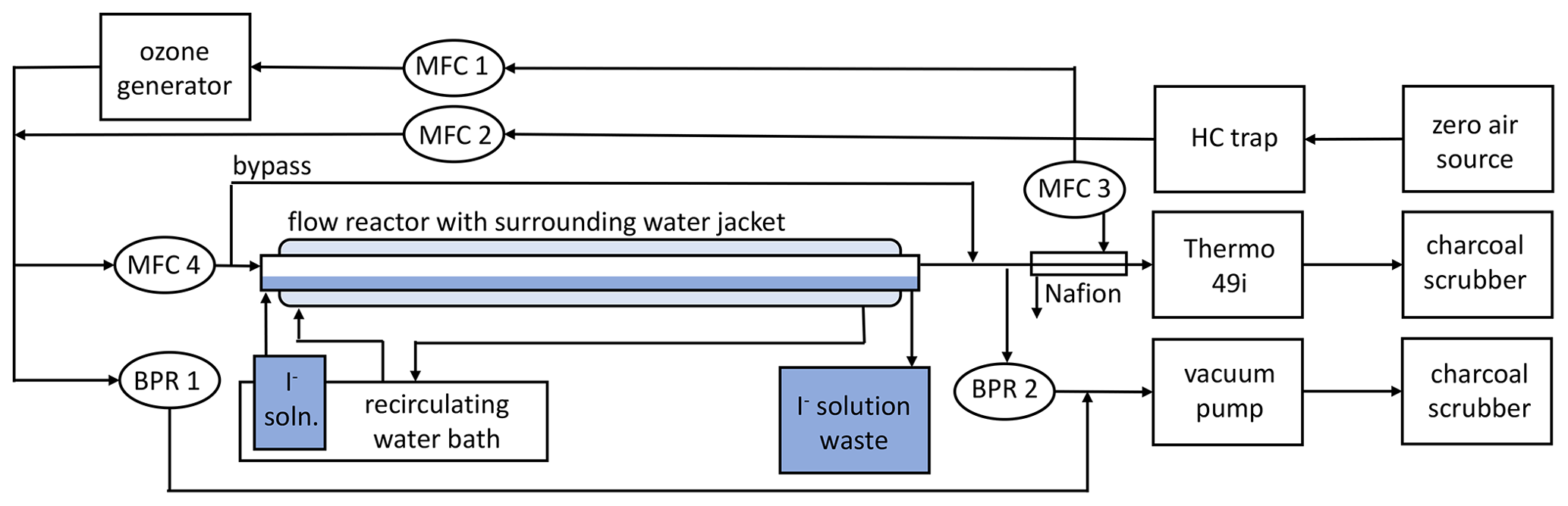
Figure 1Schematic of the experimental setup. MFC: mass flow controller; BPR: back pressure regulator.
2.1.2 Gas flow control
A temperature-controlled kinetic heterogeneous flow reactor (Fig. 1) was designed in order to enable variable flow rates of ozone and, hence, variable exposure times over iodide solutions. Hydrocarbon-filtered dry air was separated into three flows: ozonised air controlled by mass flow controller 1 (MFC 1; Alicat Scientific; MC-10SLPM-D/CM, CIN), a diluent flow (MFC 2; Alicat Scientific; MCP-50SLPM-D/5M) and a third flow diverted to a Nafion dryer (MFC 3; Aalborg Instruments; GFC 17). The combination of flows from MFC1 and MFC2 enabled the generation of a large total flow of ozone-enriched air with a constant ozone concentration. This ozone-enriched air was passed through either the flow reactor or a bypass line (MFC 4; Alicat Scientific; pc-30PSIA-D-PCV65/5P); any excess was removed through a back pressure regulator (BPR 1; Alicat Scientific; PCP-100PSIG-D/5P). Downstream of the flow tube, the gas was dehumidified using a Nafion dryer (Perma Pure; MD-110-12F-4) and analysed by the ozone monitor (∼ 1.4 slpm). Gas surplus to the analytical requirement was removed from the system by BPR 2 (15.0 psi), which was a modified MFC (Alicat Scientific; MCP-10SLPM-D/CM). This was modified using absolute pressure as the process variable and moving the valve downstream of the pressure sensor. The valve action was then inverted, meaning an increase in pressure in the flow reactor would cause an opening of the valve, allowing for constant pressure to be maintained. All ozone-containing gas was passed through a charcoal scrubber prior to venting. The ozone monitor was logged using DAQFactory, and all Alicat Scientific MFCs and BPRs were controlled and logged with DAQFactory (AzeoTech).
2.1.3 Temperature and fluid control
The flow reactor was temperature-controlled by a water jacket, supplied by a recirculating water bath chiller (TX150 and R3; Grant Instruments). The iodide or blank solutions were held within the reservoir of this water bath to equilibrate their temperature. In order to minimise any depletion of iodide from the solution during exposure to ozone, it was continuously pumped into the flow reactor using a peristaltic pump (100 series; Watson-Marlow) via chemically resistant flexible tubing (Marprene; Watson-Marlow). Once it passed through the flow tube, the iodide solution drained into a sealed, pressure-equilibrated waste bottle.
To estimate the iodide depletion during the course of the experiment with no replenishment, the rate of loss of iodide, , was calculated from the second-order rate constant for ozone and iodide and the molar concentrations of iodide and ozone in the reacto-diffusive layer of ozone (Eq. 3). In these calculations, = 1.2 × 10⁹ was used (Liu et al., 2001). The reacto-diffusive depth of ozone, δ, is the thickness of the layer in which the ozone–iodide reaction can occur (Davidovits et al., 2006), calculated by Eq. (4). Daq is the molecular diffusivity of ozone in water (1.90 × 10⁻⁹ m2 s−1 at 298 K), calculated using the temperature-dependent relationship Eq. (5), where T is the temperature in kelvin (Johnson and Davis, 1996). The reacto-diffusive depth multiplied by the surface area of the liquid gives the liquid volume in the flow reactor in which ozone is available for reaction, Vδ (Eq. 6). Assuming a worst-case scenario where mechanical turbulence from stirrer bars was not sufficient to replenish any iodide from the bulk solution into the reacto-diffusive layer, the total molar quantity of iodide available for reaction () was calculated by Eq. (7). Total loss of iodide during the total experiment time was calculated by Eq. (8), and the potential percent loss of iodide was therefore calculated by Eq. (9). Where the expected loss of iodide was greater than 10 %, the solution was pumped through the flow reactor sufficiently fast to give a residence time (Eq. 10) which, when applied in Eqs. (8) and (9), gave an I− percentage loss of < 10 %. Pump rates therefore varied with iodide concentration; however, it was verified experimentally that pump rate did not affect deposition velocity within the flow tube.
2.1.4 Measurement of aqueous iodide
Iodide concentrations in the reservoir and the waste stream were directly quantified using UV–vis spectrophotometry at 226 nM following ion exchange chromatography (IC) (Jones et al., 2023). The IC used a Dionex IonPac AS23 guard and analytical column (4 × 250 mm), with a mobile-phase eluent of 0.4 M NaCl flowing at 0.64 mL min−1. The sample injection volume was 400 µl, run time was 16.1 min and iodide was detected at 11.8 min. Samples were frozen at the time of the experiment and defrosted prior to batch analysis.
2.2 Determining surface resistance and ozone uptake
To measure surface resistance, ozone-containing gas ([O3]starting = 40 ppb) was passed over the buffered blank solution or iodide solutions that were pumped through the reactor at liquid flow rates of between 9–35 mL min−1. Gaseous flow rates were set at 1600, 1900, 2400, 3200 and 4500 sccm, giving possible ozone–solution reaction times ranging from 20–66 s (reaction time = headspace volumeflow rate). The buffered phosphate solution was pre-ozonised by passing a high concentration of ozone (approx. 200 ppb) over the solution in the flow reactor. The total volume of buffer solution required for the experiment was circulated through the reservoir and flow reactor during this time to ensure the entire solution was pre-ozonised. This was continued until a stable ozone concentration was obtained, which typically took around 1 h. At this point the glass, tubing, fittings and buffer were considered “conditioned”. The ozone concentration was lowered to the desired experimental concentration measured while flowing through the bypass line, which had also been pre-conditioned with ozone. The blank measurement was then carried out over the buffer solution, which was pumping through the flow reactor. Blanks were performed in duplicate or triplicate. Directly following the blank measurement, the solution was spiked with iodide into the reservoir, and the solution was mixed and circulated through the flow reactor for approximately 10 min to ensure homogeneity. During mixing, the ozone was passed through the bypass line to avoid reaction. The iodide measurement was performed directly after mixing in triplicate. An example experiment output is shown in Fig. 2.
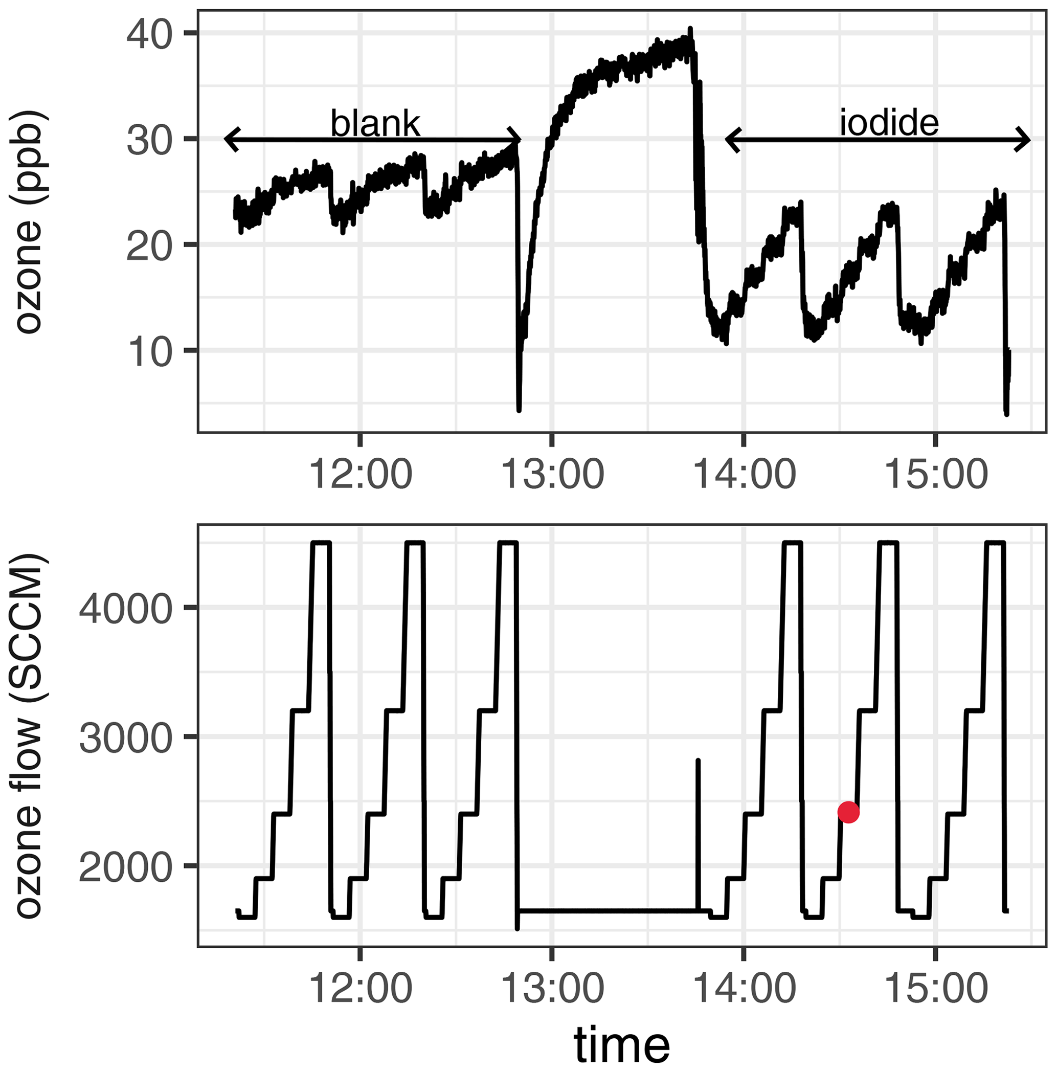
Figure 2Experimental output for a typical measurement, including residual ozone measured downstream of the flow tube and the concurrent flow rate of ozone over the solution. A blank measurement and the measurement following iodide spiking are shown. The red-filled circle indicates the timing of the collection of the iodide “midpoint” sample from the waste stream. Experimental conditions: T = 303 K, [I−] = 633 nM, phosphate buffer (10 mM; pH = 8), [O3]starting = 40 ppb.
Residual ozone was measured after each reaction time, and a mean ozone concentration for each reaction time was obtained ([O3]). A plot of ln[O3] against reaction time (Fig. 3) yielded a linear trend, the gradient of which was calculated for each repeat of both the blank (mblank) and the iodide-containing samples (msample), which were each averaged. A blank-corrected gradient (mcorrected, Eq. 11) was used to calculate vd by Eq. (12), where V is the headspace volume and SA is the liquid surface area (values for all physical constants and metadata provided in Appendix A and calculations described in Appendix B).
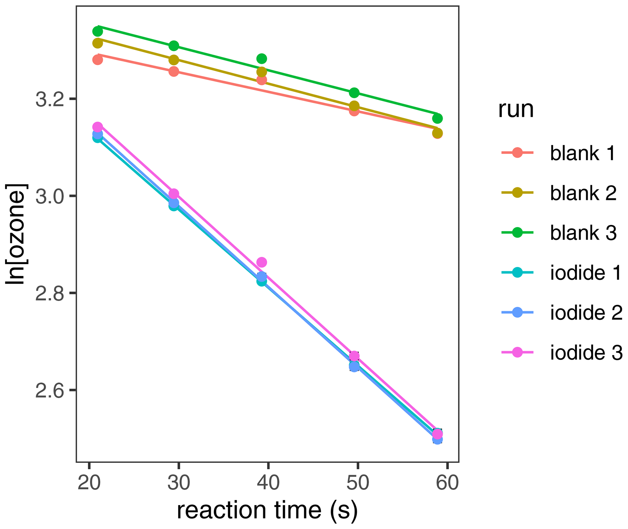
Figure 3ln[O3] against reaction time for experimental conditions: T = 303 K, [I−] = 633 nM, phosphate buffer (10 mM; pH = 8), [O3]starting = 40 ppb.
Total resistance, rt, is the inverse of gas-phase corrected vd, from which rs can be calculated (Eq. 1). The value of ra is variable in the environment but constant in the controlled environment of the flow reactor. Measured over a high iodide concentration (0.02 M), it is assumed that there is negligible surface resistance; therefore, ≈ (Galbally and Roy, 1980). When measured for this flow reactor, an ra of 6.6 ± 0.14 s cm−1 was obtained. This value was subtracted from total resistance measured for each sample.
The relationship between the second-order rate constant, , and rs was defined by Eq. (2), where H is the temperature-dependent dimensionless Henry's law coefficient of ozone (Hgas/aqueous = 3.63 at 298 K), calculated using Eq. (13) (Kosak-Channing and Helz, 1983); T is the solution temperature (K); and μ is the molar ionic strength (≈ molar concentration, at the concentrations used in this work). To apply Eq. (2) to our measurements, for each temperature applied, a plot of against gave a linear relationship (see “Results and discussion”; Fig. 5), from which the gradient, m, was used to calculate , according to Eq. (14).
3.1 Kinetics and temperature dependence of the ozone–iodide reaction
Conditions within the flow reactor were chosen to emulate the remote marine surface ocean and atmospheric boundary layer. The mixing ratio of ozone in air was not expected to affect ozone uptake to iodide solution as, under these conditions, a bulk aqueous reaction between ozone and iodide is anticipated, for which a lack of ozone dependence is characteristic. Dependence of uptake on the mixing ratio of ozone would be expected if the reaction were proceeding via a surface-mediated Langmuir–Hinshelwood reaction. This is due to surface saturation of ozone at higher mixing ratios limiting potential reactivity on the surface. Therefore, a greater ozone uptake would be expected at lower ozone mixing ratios. Under the conditions of our experiments, there was no significant dependence of deposition velocity on the ozone mixing ratio (Fig. 4; p=0.74), confirming the reaction occurs in the bulk phase under the conditions employed. Despite the lack of dependence of ozone mixing ratio on reactivity, consistent conditions of 40 ppb ozone were used in each experiment to mimic a typical mixing ratio of ozone in the troposphere. Similarly, although there is evidence that pH has no impact on ozone deposition to iodide solutions (Schneider et al., 2022), the solutions were buffered to pH 8 to mimic typical oceanic alkalinity.
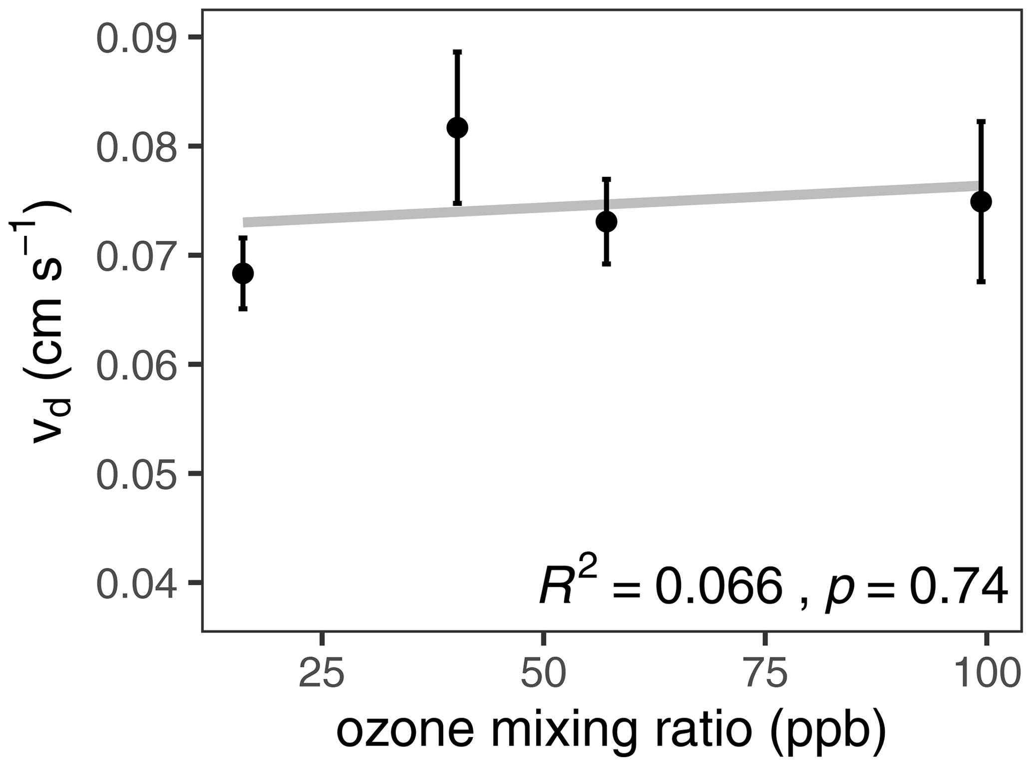
Figure 4Deposition velocity as a function of ozone mixing ratio over iodide in phosphate buffer (10 mM; pH = 8). Mean [I−] = 1.79 µM (1.70, 1.73, 1.93 and 1.79 µM from lowest to highest ozone mixing ratio); T = 298 K.
Iodide was the reagent in excess in the pseudo-first-order conditions sought for kinetic analysis. At the low iodide concentrations required to emulate marine conditions, iodide was expected to be depleted during the ∼ 90 min experiment time (Schneider et al., 2020); therefore, the liquid phase in the flow reactor was continuously replenished from a reservoir, passing through the flow reactor and out to waste. To verify that the chosen pump rate was sufficient to keep iodide depletion below 10 % during the residence time of the liquid in the reactor, liquid samples were collected before and after being exposed to ozone in the flow reactor. The sample after the flow reactor was taken at the midpoint of the experiment (ozone flow rate 3 of 5 and during run 2 of 3; indicated by the red circle in Fig. 2). For all reported experiments, the iodide concentration after the experiment was verified by liquid chromatography. It was confirmed that the concentration during the midpoint of the experiment, taken to represent average iodide loss across all ozone exposure times, had less than a 10 % difference from the starting concentration (Appendix C). For all further analysis, the iodide concentrations reported are the midpoint values, rather than the starting values, to best represent the average conditions of the experiments.
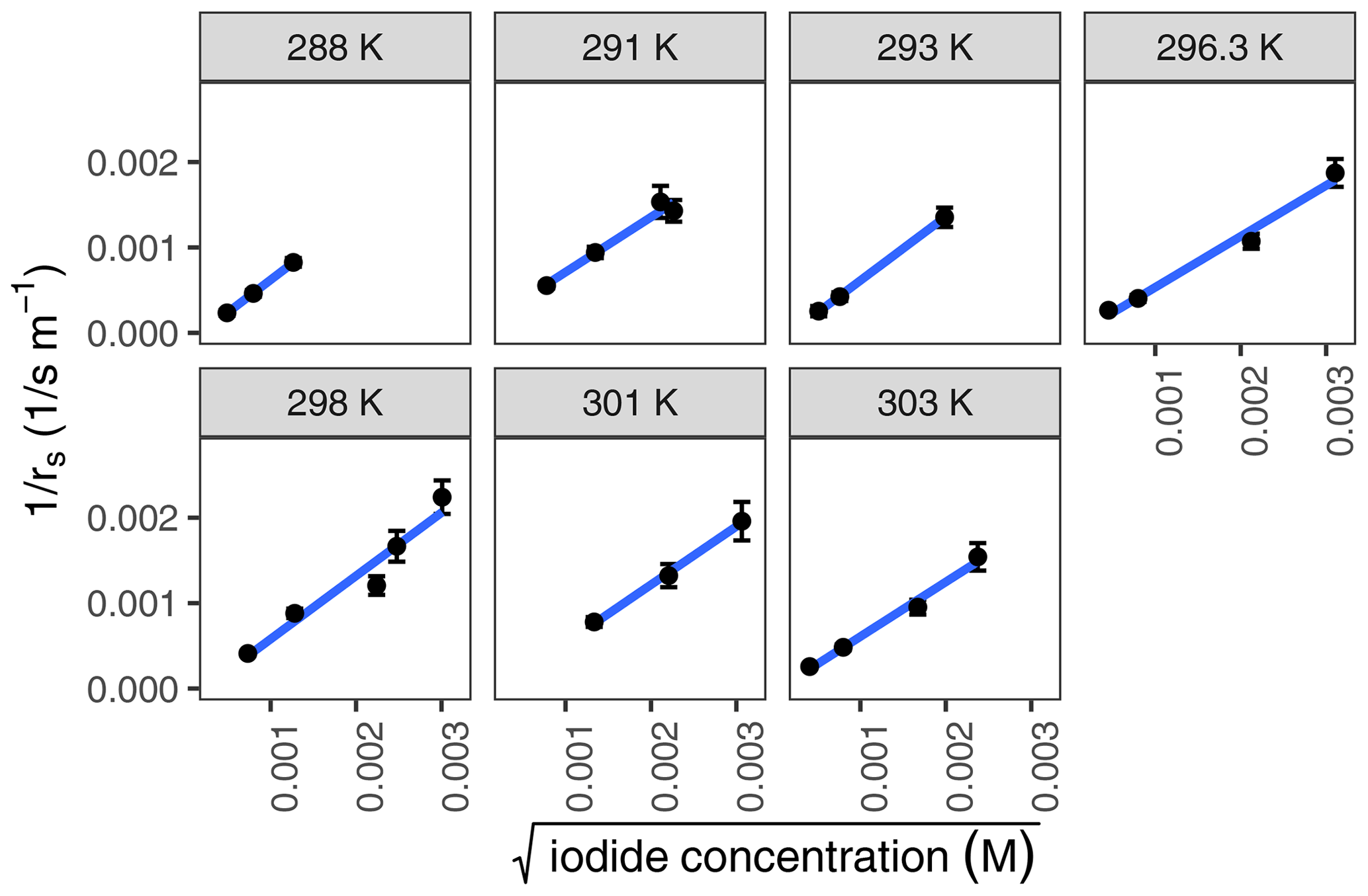
Figure 5Inverse of rs calculated for various iodide concentrations (102 nM–9.88 µM) at temperatures between 288 and 303 K. Measurements were performed in triplicate, and error bars were propagated from the ra error, the standard error in linear fit from experimental output, and the errors in the measurements of liquid volume and flow tube dimensions.
The second-order rate constant for ozone with iodide was measured for iodide concentrations between 102 nM and 9.88 µM and for water temperatures between 288 and 303 K (Fig. 5). Results were compiled to an Arrhenius plot (Fig. 6), leading to a calculated pre-exponential factor, A, of 5.4 ± 23.0 × 10¹¹ and activation energy, Ea, of 7.0 ± 10.5 kJ mol−1. The Pearson correlation coefficient of the Arrhenius plot indicated that the trend was not statistically significant (p=0.53). Therefore, the null hypothesis cannot be rejected; i.e. we cannot conclude that the reaction between ozone and iodide is dependent on temperature.
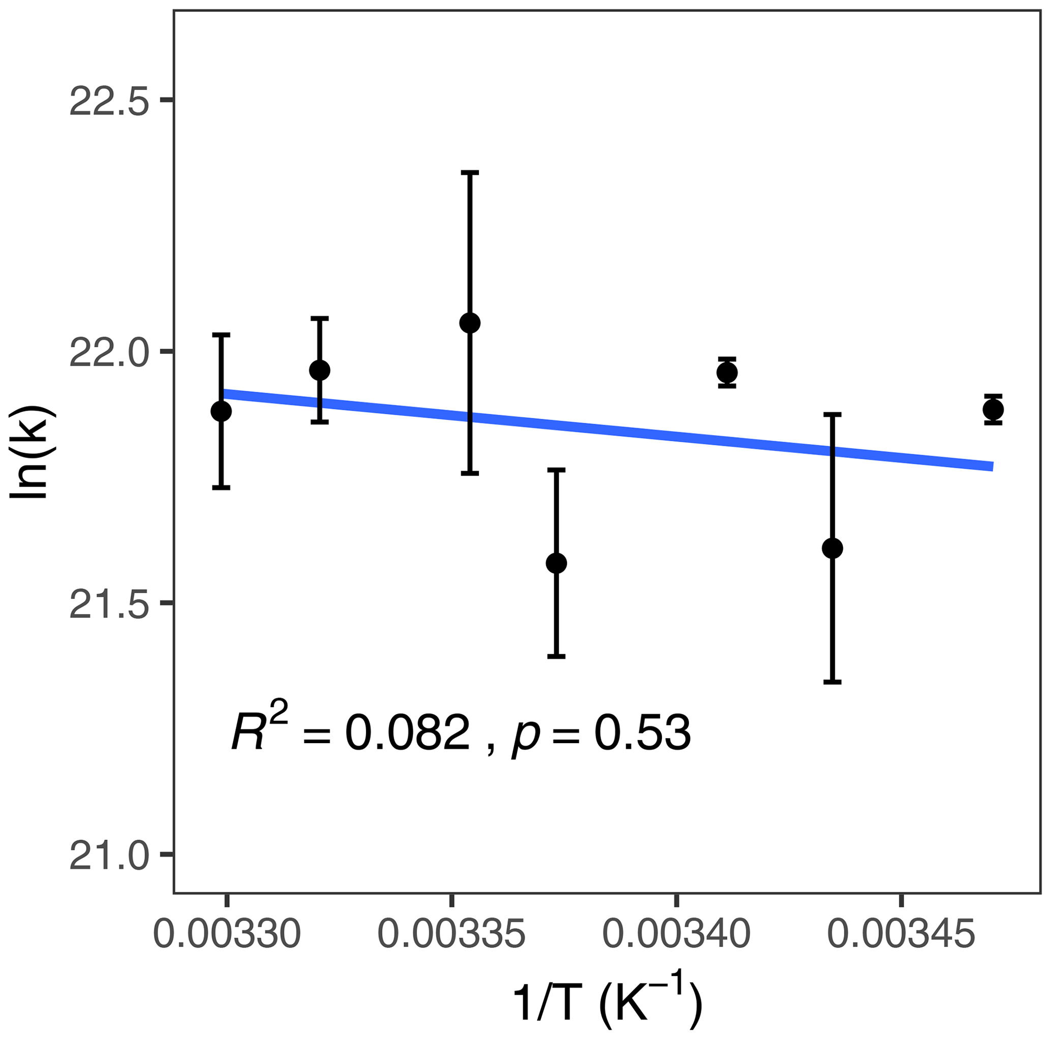
Figure 6Arrhenius plot for the reaction between ozone and iodide; the linear correlation has a p=0.53 and R2 = 0.082. Error bars represent the standard error in the linear fit of vs. [I−] for each temperature.
The blank measurement was subtracted from the iodide-containing measurement (Eq. 11), to account for ozone loss to the phosphate buffer and to the glass walls and fittings. It should be noted that if ozone loss during the blank measurement were to be occurring due to reactions outside the iodide-containing reacto-diffusive length, this could cause our measurements to be an underestimation of the true reaction rate.
Garland et al. (1980)Hu et al. (1995)Magi et al. (1997)Liu et al. (2001)Rouvière et al. (2010)Shaw and Carpenter (2013)Table 1Results and conditions of previous kinetic studies on the reaction between ozone and iodide. The symbol – denotes that the condition was not reported.
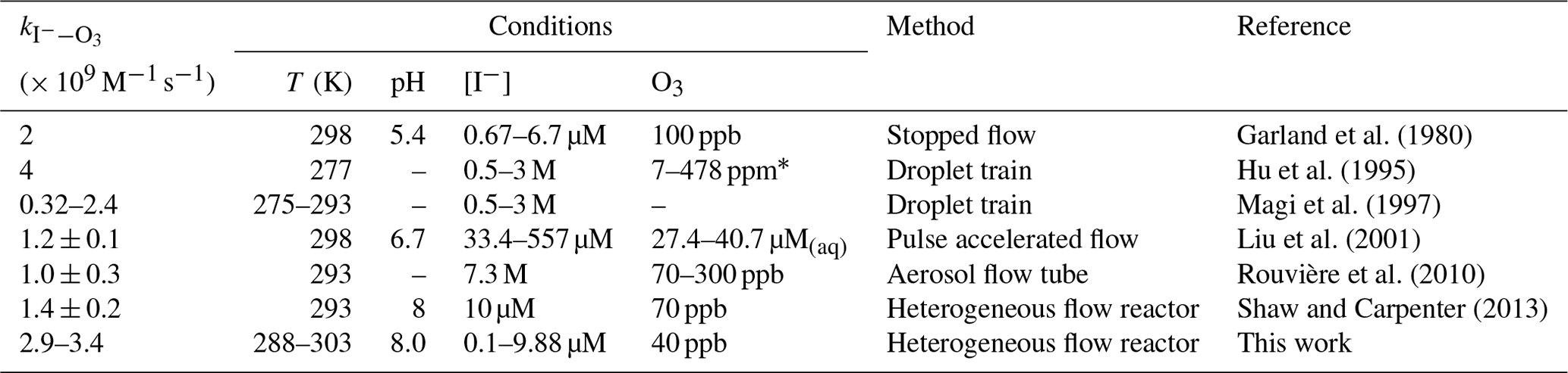
∗ 5 × 10¹²–1 × 1014 cm−3 ozone reported; converted to ppm (6–20 Torr; 277 K).
Several studies have measured the second-order rate constant at around room temperature, as compiled in Table 1. The rate constants obtained from these studies are plotted as a function of temperature in Fig. 7. Based on experimental conditions and relevance to marine environments, the studies which are most comparable to ours are those which employ iodide concentrations below 10−4 M (Moreno et al., 2018); these are Garland et al. (1980), Liu et al. (2001), and Shaw and Carpenter (2013). The study by Liu et al. (2001) was carried out with iodide concentrations approaching the upper limit of where aqueous reactivity dominates, but ozone was applied in solution, removing the possibility of surface reactivity. Garland et al. (1980), Liu et al. (2001), and Shaw and Carpenter (2013) report a comparable but slightly lower than this work. A possible reason for this could be the lack of replenishment of iodide in their studies. Iodide depletion could occur within the timeframe of their experiments, which would have resulted in a rate of ozone loss lower than anticipated for their expected iodide concentration. Iodide was not explicitly measured in those studies, so any depletion would not be known. For all other reported rate constants, the conditions employed could promote surface reactivity; therefore, the measurements are not comparable to the results reported in this work.
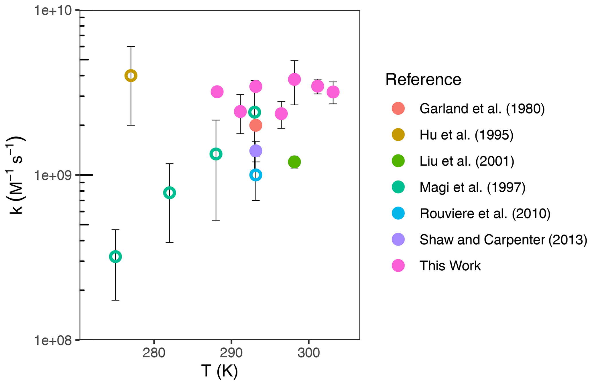
Figure 7Compilation of literature-reported second-order rate constants between ozone and iodide as a function of temperature. For Hu et al. (1995), errors were not reported; error bars shown are a lower-limit estimate based on statements made in the text. Filled circles indicate experiments performed with environmentally relevant conditions. Empty circles (◦) indicate experiments which are not environmentally applicable.
Of the various reported rate constants for the ozone iodide reaction (Table 1 and Fig. 7), only one other study has explicitly investigated the temperature dependence and obtained A = 1.4 × 10²² and Ea = 73.08 kJ mol−1, with an estimated error of 40 % (Magi et al., 1997). Our work contradicts the strong positive temperature dependence reported in their work. The difference in conclusion could be due to the differences in conditions. At the concentrations used in our study, bulk reactivity is expected to occur, whereas the conditions employed by Magi et al. (1997) (iodide concentrations of up to 3 M) are in a range which could display surface reactivity. The surface reactivity is also dependent on the gaseous ozone concentration, which was not reported. Further, while interfacial reactivity is not yet fully understood, the pre-exponential factor reported by Magi et al. (1997) is approximately 12 orders of magnitude greater than a diffusion-controlled reaction. In contrast, the pre-exponential factor reported in our work could feasibly be attributed to a diffusion-controlled reaction, within error bounds.
Amalgamating results of single-temperature studies by Hu et al. (1995), at 277 K, and the room temperature measurements of Garland et al. (1980), Liu et al. (2001), Rouvière et al. (2010), and Shaw and Carpenter (2013), as well as this study, yields a negligible or slightly negative temperature dependence, within the associated experimental errors, for the bulk-phase reaction between ozone and iodide (Fig. 7). Comparing only those experiments which are environmentally applicable, there is no clear trend in temperature dependence. Both conclusions are consistent with the results of our study.
Theoretical studies of this reaction have previously been performed. One study simulating the aqueous phase concluded a strong positive activation energy (20 kcal mol−1 or approx. 84 kJ mol−1) for the formation of intermediate complex [OOOI]− (Eq. R1), acting as the rate-limiting step (Gálvez et al., 2016). A subsequent gas-phase simulation concluded a weaker but still positive activation energy of 7.5 kcal mol−1 or approx. 32 kJ mol−1 for the same adduct formation (Teiwes et al., 2018). These values are in contradiction with the results of this experimental study, and if the energetic barrier to this reaction is indeed adduct formation, our results indicate this barrier is overestimated by computational studies. Therefore, we propose that further work is required to reconcile mechanistic theory with observations.
3.2 Application to previous laboratory measurements of iodine emissions
A previous laboratory study of inorganic iodine (HOI and I2) emissions from ozonised iodide solutions (0.1–5 µM iodide; 222–3600 ppb ozone; temperature of 276–298 K) yielded effective activation energies of 17 ± 50 kJ mol−1 for HOI emissions and −7 ± 18 kJ mol−1 for I2 emissions (MacDonald et al., 2014). The emissions of HOI and I2 depend on several chemical reactions, each with individual dependencies on temperature, and several physical factors including the solubility and diffusivity of ozone. Thus, the temperature dependence can be negative or positive depending on the combination of these factors. The MacDonald et al. (2014) study was carried out in conditions favouring bulk-phase reactions between ozone and iodide, making their results experimentally comparable to our work. When MacDonald et al. (2014) modelled the emissions of HOI and I2, they demonstrated that their results could only be accurately replicated when assuming that Ea ∼ 0 kJ mol−1 for the ozone–iodide reaction and not when using the temperature dependence from Magi et al. (1997). The model employed by MacDonald et al. (2014) was the sea surface microlayer (SML) model described by Carpenter et al. (2013), except with the inclusion of temperature-dependent processes. The model with temperature dependence did not account for iodine depletion following its fast reaction with ozone and did not account for iodide replenishment from the waters below (Schneider et al., 2020). To evaluate whether the rate coefficient obtained in our experimental work is consistent with the measured temperature dependence of fluxes of gaseous iodine compounds from iodide solution under ozone, we applied our rate coefficients to an updated SML model (Pound et al., 2023). The updated SML model (details in Appendix D) includes the mixing of iodide between the SML and the underlying water and simulates surface iodide depletion, especially at low wind speeds and/or reduced turbulence. The depth of the SML in this model is defined as the reacto-diffusive length of ozone, which is unique to each combination of conditions.
The SML model was constrained to the range of conditions reported by MacDonald et al. (2014). The effective activation energy was calculated (Ea = ) from an Arrhenius-type plot of the natural log of the calculated emissions of HOI and I2 (in units of ) against the inverse of the temperature (in K). It was not possible to accurately calculate an equivalent wind speed for the MacDonald laboratory experiments; therefore, two low wind speeds (0.005 and 0.03 m s−1) were assumed. When assessing the impact of different wind speeds, we applied conditions of 1500 ppb ozone and 2.5 µM iodide.
The HOI and I2 emissions obtained from the updated SML model are displayed as an effective Arrhenius plot in Fig. 8. The modelled emissions indicate there is a dependence of the effective activation energy on the wind speed of the experiments for I2 emissions. At the higher wind speed, the model overestimates the activation energy, outside the error range of the experimental measurements. The lower wind speed predicts an Ea within the experimental error range. For HOI emissions, a slightly negative Ea is predicted by the model, which lies within the experimental error range quoted by MacDonald et al. (2014), and does not show a dependence on wind speed.
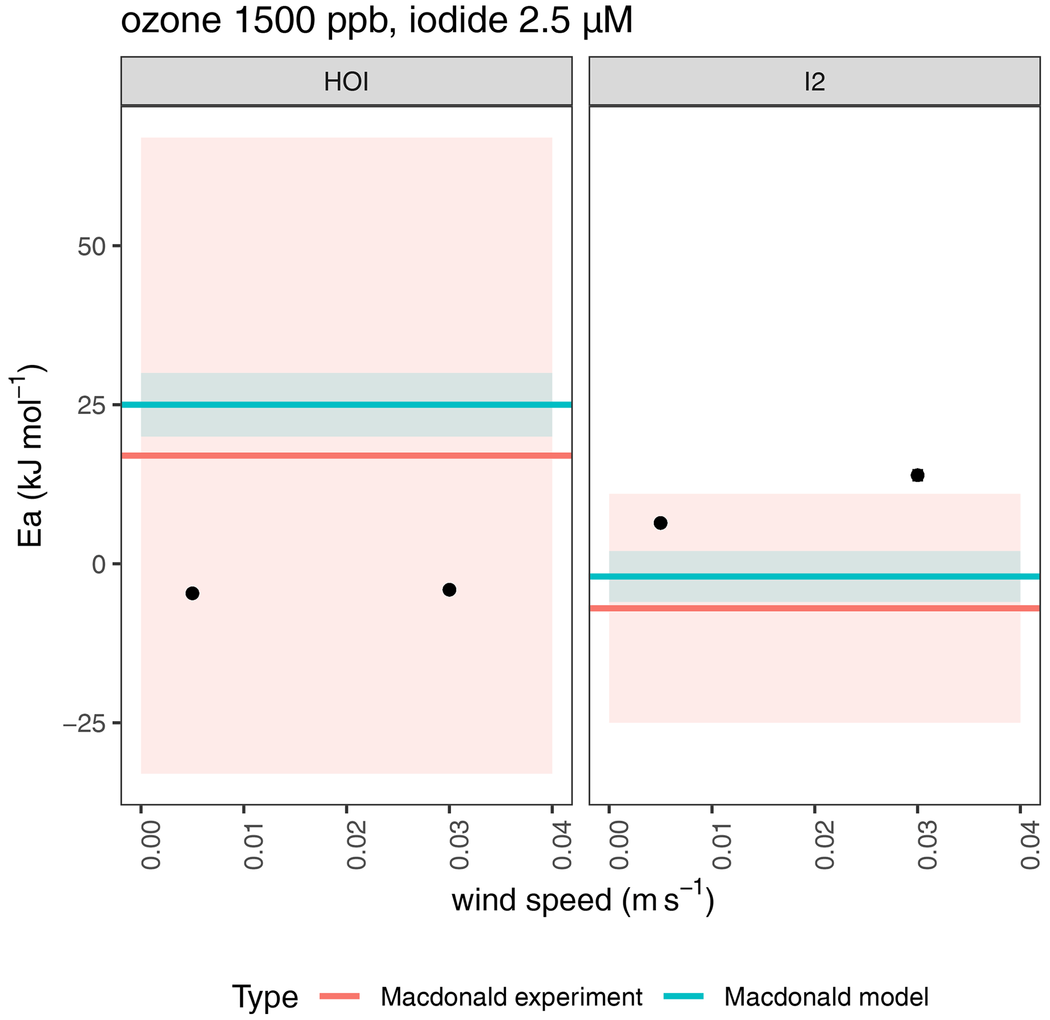
Figure 8Effective activation energies for emissions of HOI and I2 from ozone oxidation (1500 ppb) of iodide solution (2.5 µM) as a function of wind speed. Points show modelled emissions using the SML model (Pound et al., 2023), while horizontal red and blue lines show experimental and modelled emissions, respectively, from MacDonald et al. (2014). Errors are shown by shaded areas, and reflect the standard error in the linear fit from modelled output.
Knowing that there is negligible temperature dependence on the reaction between iodine and ozone, the relative changes in each step of the production and emission of HOI and I2 in the Pound et al. (2023) SML model were interrogated to explain the predicted activation energies. Iodide in the surface layer is depleted if the replenishment from the bulk solution occurs at a slower rate than the reaction of iodide with ozone. Iodide depletion was modelled over the range of ozone, iodide and temperature reported by MacDonald et al. (2014), and depletion was predicted to increase with increasing ozone concentration and wind speed and with decreasing iodide concentration and slightly decrease with temperature (Fig. 9). The SML model shows that iodide depletion increases with increasing ozone concentration and with decreasing iodide concentrations due to the chemical consumption of the available iodide. Greater depletion is seen at the higher wind speed because of the increase in ozone deposition as aerodynamic resistance (ra) is reduced with higher air-side turbulence (vd = 0.0013 cm s−1 at 0.03 m s−1 and vd = 0.0003 cm s−1 at 0.005 m s−1). Waterside transfer velocity, kw, which replenishes iodide from the bulk to the SML, is still low at these wind speeds and does not offset the increase in ozone–iodide reactivity; therefore, iodide is seen to be more depleted at 0.03 m s−1 compared to 0.005 m s−1. This is the opposite to what we expect in the environment, where greater wind speeds would be associated with a greater degree of mixing from the bulk and less iodide depletion. This is discussed in detail in Pound et al. (2023). The trend with wind speed we describe in the current work is specific to low-wind-speed laboratory conditions. This should therefore be considered in future experimental design if environmentally applicable emission data are sought.
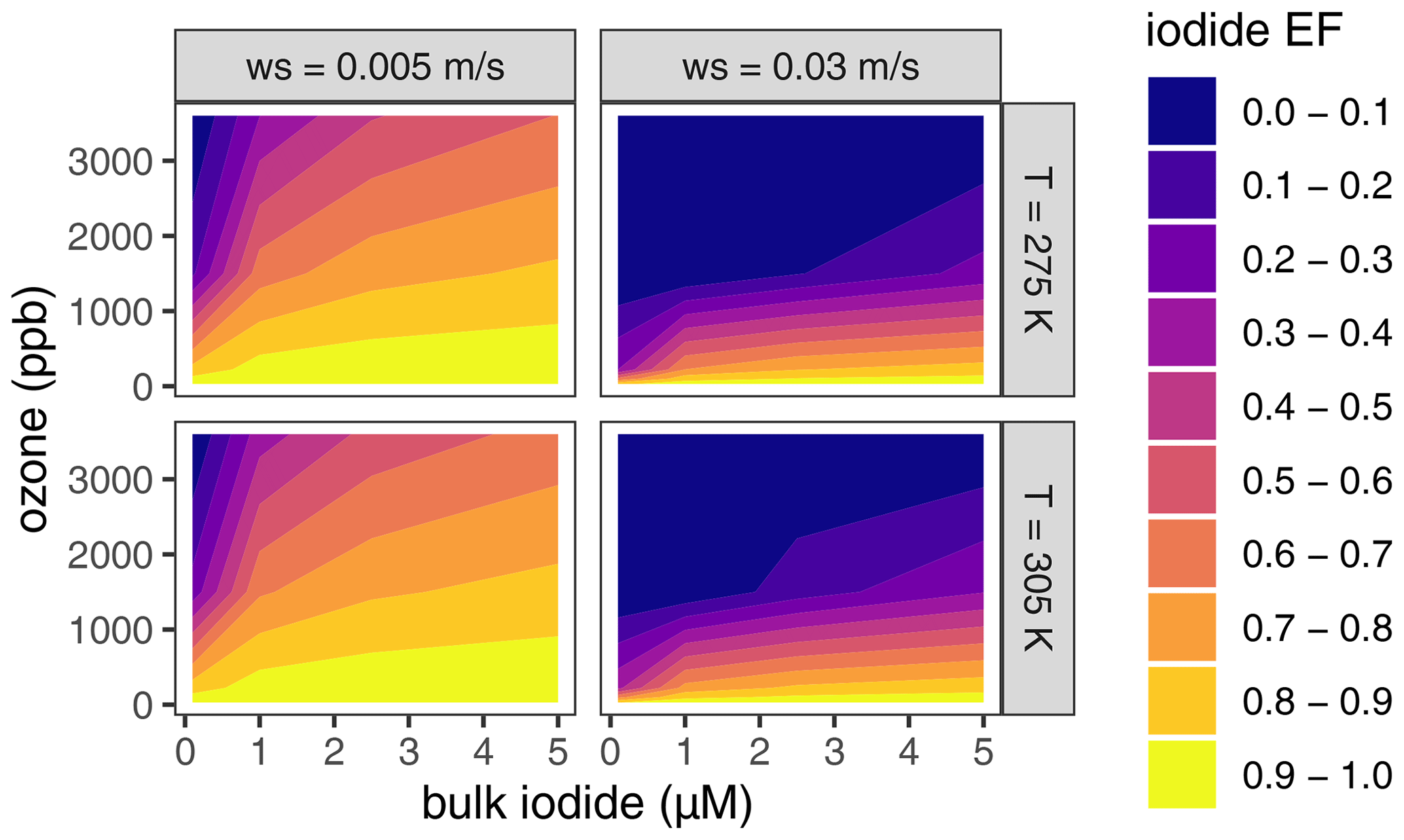
Figure 9Modelled iodide depletion for ozone-oxidised iodide solution, under the following conditions: 0.1–5 µM [iodide]; 222–3600 ppb ozone; T = 276–298 K. Iodide enrichment factor (EF) = .
The SML model predicted iodide depletion to slightly decrease with temperature; that is, we predict a higher iodide concentration in the SML at higher temperature given equal wind speed and ozone concentration. This is due to the small positive temperature dependence in the ozone–iodide reaction being offset by the increase in kw with temperature, which increases the mixing of iodide from the bulk to the SML. The effect of temperature is more pronounced at higher wind speed because, though small, kw is higher at greater wind speed and therefore has greater impact at 0.03 m s−1 compared to 0.005 m s−1. This impact is minor compared to the effects of ozone, iodide and wind speed. In light of this discussion, it should be noted that there are very few observations of iodide concentrations at or proximal to the surface layer (Stolle et al., 2020), and it is this iodide which is available for reaction with ozone. Concentrations of iodide at or proximal to the surface may frequently be different from the reported bulk concentration.
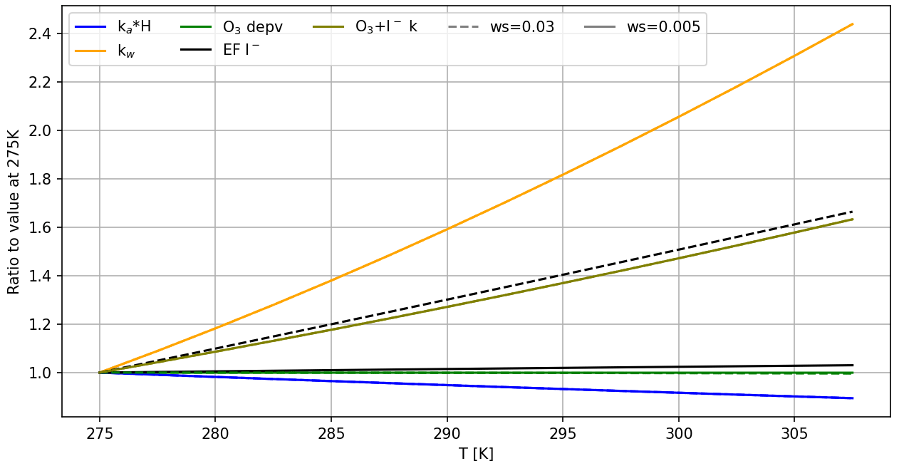
Figure 10Relative change in selected variables with respect to the lowest modelled temperature. Variables selected are those with the greatest impact on emissions of HOI. Model conditions: ozone mixing ratio = 1500 ppb; [iodide] = 2.5 µM. Values ka, kw and H are calculated for HOI. Dashed lines correspond to ws = 0.03 m s−1, and the solid lines refer to ws = 0.005 m s−1. Where the dashed line is not visible, this is because it is identical to the solid line.
For both wind speeds investigated, ozone deposition velocity was effectively constant over the modelled temperature range (Fig. 10). This is because at low wind speeds, the deposition of ozone is limited by air-side resistance, ra, which has no temperature dependence. Therefore, factors which decrease rs (e.g. changes in ozone solubility, aqueous diffusivity of ozone, and reaction rate between ozone and iodide with temperature) do not influence deposition significantly. Hence, the availability of ozone in solution was constant over the prescribed temperature range. Temperature trends in HOI emissions are therefore controlled by drivers in mixing to the bulk or drivers in Reaction (R5), which could include air-side transfer velocity, ka, and the solubility of HOI, expressed as the dimensionless Henry's law coefficient, HHOI, which is calculated using equations in Johnson (2010) and using physical constants from Thompson and Zafiriou (1983). The relative changes in selected chemical and physical drivers across the temperature range are displayed in Fig. 10. Flux into the air, Fa, is controlled by Eq. (15), where CSML and Ca are concentrations of the species in question in the SML and in the air, respectively. In this model, Ca is assumed to be zero. Across this temperature range, we expect a small decrease in the product of HHOI×ka(HOI), resulting in a lower flux of HOI into the atmosphere as T increases and hence the slight negative Ea for HOI emissions.
Due to its high solubility, the majority of HOI produced in the SML is mixed into the bulk liquid phase, Fb (Eq. 16), rather than being emitted. Here, kw is the waterside transfer velocity, and Cb is the bulk concentration, set to zero in this model. Chemical production of HOI is the only source of HOI in the SML, and the second-order rate constant of the chemical formation of HOI, , increases with temperature. At 0.03 m s−1 wind speed, this is augmented by the reduced iodide depletion with higher temperature, leading to production of more HOI. At 0.005 m s−1 wind speed, this effect is reduced by the effectively unchanging iodide depletion across the temperature range. In both instances, increased HOI production with T counteracts some of the increased loss to the bulk and more so at 0.03 m s−1 wind speed. This results in a slightly higher [HOI] in the SML at the higher temperature range, which increases the Ea slightly at the higher wind speed (−4.65 kJ mol−1 at 0.005 m s−1 compared to −4.08 kJ mol−1 at 0.03 m s−1).
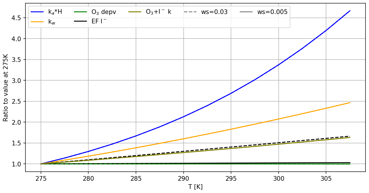
Figure 11Relative change in each variable with respect to the lowest modelled temperature. Variables selected are those with the greatest impact on the emissions of I2. Model conditions: ozone mixing ratio = 1500 ppb; [iodide] = 2.5 µM. Values ka, kw and H are calculated for I2. Dashed lines correspond to ws = 0.03 m s−1, and the solid lines refer to ws = 0.005 m s−1. Where the dashed line is not visible, this is because it is identical to the solid line.
For I2, emissions are largely controlled by its low solubility. Temperature impacts on chemical and physical drivers are displayed in Fig. 11. We calculate a strong increase in , which leads to a higher Fa at greater temperatures, and a positive Ea at both wind speeds. While the rate constant of mixing to the bulk, kb, also increases with temperature, its effect is counteracted by the increased chemical production of I2 with increased temperature, driven by increased and decreased iodide depletion. This results in a more positive Ea at the higher wind speed.
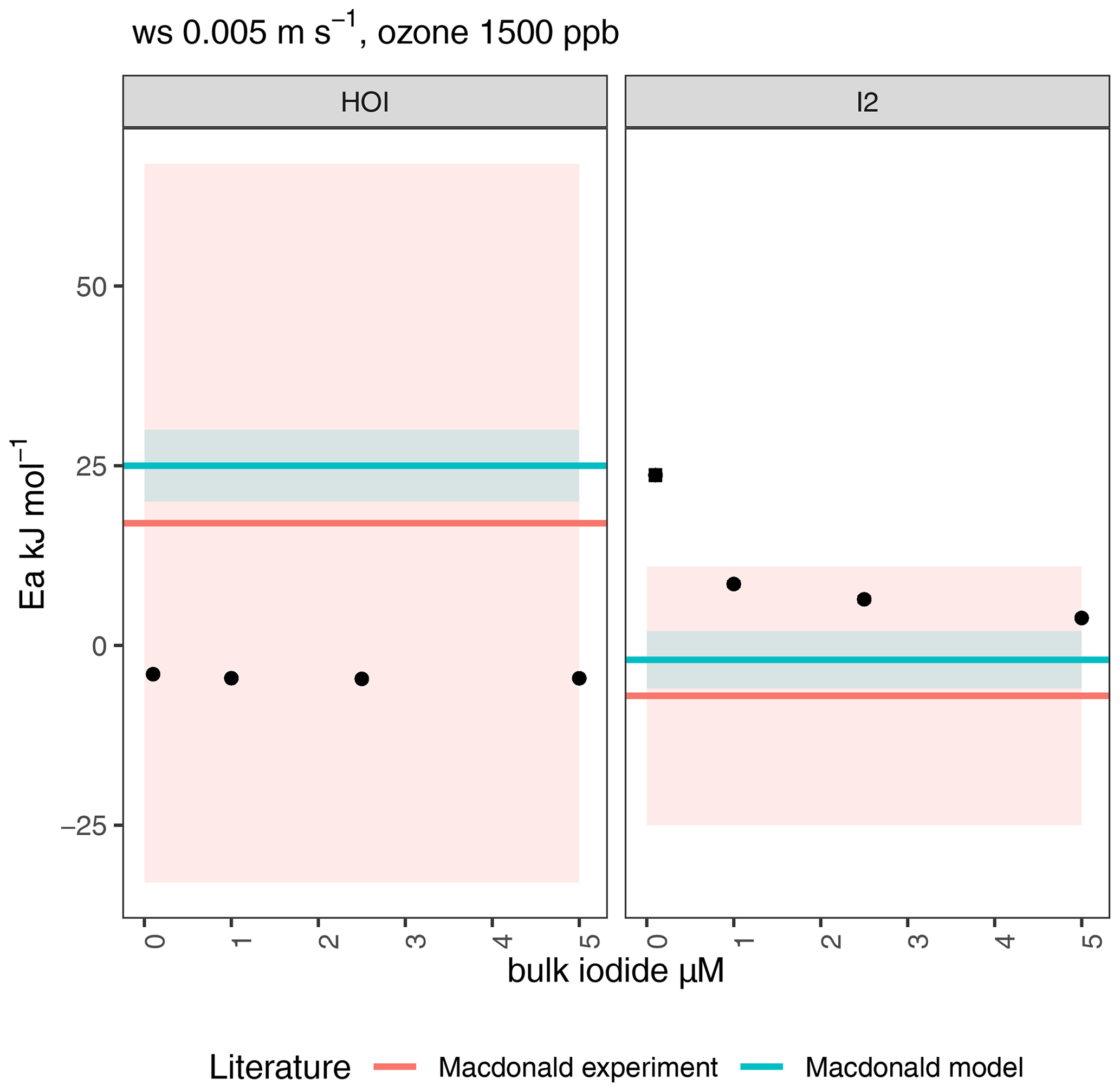
Figure 12Effective activation energies for emissions of HOI and I2 from ozone oxidation (1500 ppb; wind speed of 0.005 m s−1) of iodide solution as a function of bulk iodide concentration. Points show modelled emissions using the SML model (Pound et al., 2023), while horizontal red and blue lines show experimental and previously modelled emissions, respectively, from MacDonald et al. (2014). Errors are shown by shaded areas and reflect standard error in the linear fit from modelled output.
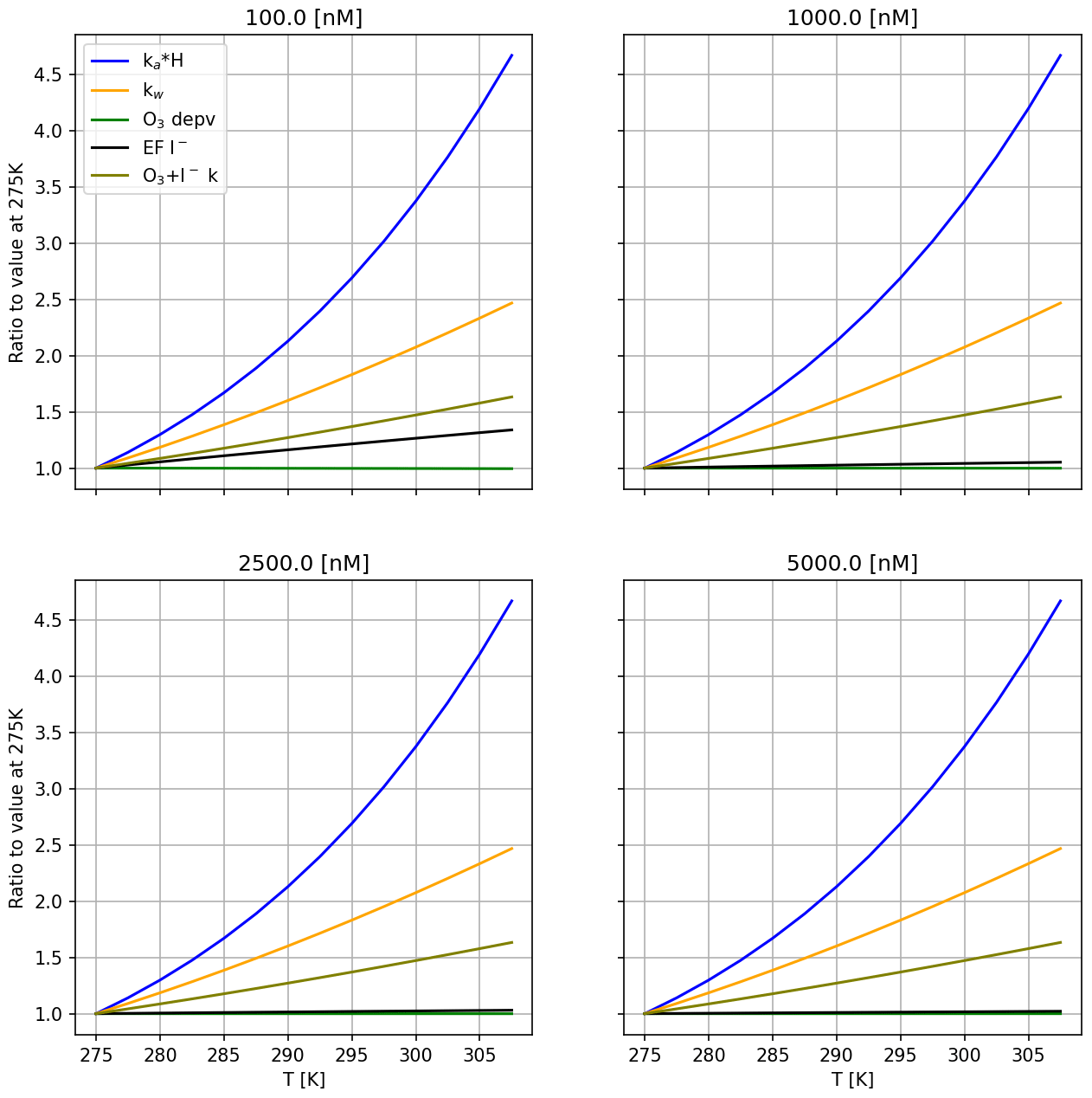
Figure 13Relative change in selected variables with respect to the lowest modelled temperature for each modelled bulk iodide concentration. Variables selected with significance for emission of I2. Model conditions: ozone mixing ratio = 1500 ppb; wind speed = 0.005 m s−1. Values ka, kw and H are calculated for I2.
The effects of varying iodide concentrations on HOI and I2 emissions were also investigated at a wind speed of 0.005 m s−1 due to the model's better comparability to experimental results at this wind speed. The calculated activation energies are displayed in Fig. 12. For the range of iodide concentrations used in MacDonald et al. (2014), we calculate that the Ea of HOI emissions has no dependence on iodide and remains slightly negative for all modelled conditions (driven by increased mixing to the bulk at higher temperature, as above). For I2 emissions, the modelled Ea was more strongly positive at the lowest iodide concentration due to greater iodide depletion in the SML. The iodide limitation is counteracted at higher temperatures by increased mixing from the bulk. In Fig. 13, it can be observed that for 100 nM iodide, the iodide enrichment factor increases with temperature, which is not observed for the other iodide concentrations. This results in a more strongly positive Ea at the lowest modelled iodide concentration of 100 nM, which is comparable to conditions found in the environment. We therefore believe that the activation energy of I2 emissions reported in MacDonald et al. (2014) may underestimate the temperature dependence of oceanic I2 emissions.
The model was also used to test for ozone sensitivity; however, across the range studied here, the ozone mixing ratio was not determined to influence activation energy for HOI or I2 emissions.
It is important to note that there are large uncertainties present in calculating gas and water transfer coefficients (ka and kw), quoted as up to a factor of 2 (Johnson, 2010). Furthermore, there are also large uncertainties in the solubilities of HOI and I2; for example, the Henry's law coefficient of HOI is assumed to be within the range of 0.44 to 440 (Thompson and Zafiriou, 1983). Uncertainties in kw, ka and H are not included in this analysis as they are not accurately quantified, nor is it clear how they relate to iodine emissions. An additional caveat in comparing the SML model to laboratory studies is that the model was designed for application to environmental settings and therefore is not optimised for the low wind speeds and high ozone and iodide concentrations explored in this work.
A thorough understanding of the kinetics of the reaction between ozone and iodide in oceanic systems is important for predicting and understanding tropospheric ozone concentrations in remote ocean regions. The second-order rate constant of the reaction between ozone and iodide and its temperature dependence were measured in this work using a variable flow methodology, under conditions which emulate the bulk kinetics expected in the surface ocean. A negligible, non-statistically significant temperature dependence was obtained, contradicting a previous study. We therefore conclude that the temperature dependence of this reaction in the ocean has previously been overestimated.
Though a lack of temperature dependence has previously been implied by comparison between studies and by back-calculating from emissions, this is the first study, to our knowledge, to show this by direct measurement. The temperature dependence obtained was used to replicate and explore results produced from a previous laboratory study of HOI and I2 emissions from an iodide solution exposed to ozone. This result has implications for oceanic ozone deposition and emissions of gaseous iodine species to the troposphere (Carpenter et al., 2013). Despite being outside of the temperature range studied here, this work has potential further implications for halogen emissions to the stratosphere (Koenig et al., 2020). In related work, we have incorporated these kinetics into a global transport model, the GEOS-Chem model, to improve our understanding of ozone in the troposphere.
This work also demonstrates that the laboratory-measured temperature dependence of I2 and HOI emissions, which are a result of complex interactions between physical and chemical parameters, is highly dependent on experimental conditions (including both iodide concentration and wind speed) and therefore cannot easily be translated into ambient emissions. It is noteworthy that the wind speeds applied in our and other authors' experiments are not comparable to those found in the environment. In particular, the very low or negligible water turbulence accessible in laboratory experiments is far lower than that typically found in the ocean. The result of this is that while we simulate increasing iodide depletion in the surface layer with “wind speed” at very low wind speeds, this is not typically expected in the environment where we predict that iodide depletion decreases with increasing wind speed (Pound et al., 2023). The latter is a result of greater wind-induced turbulence increasing the rate of iodide replenishment from the bulk to the surface layer. We also find that such iodide depletion in the SML, as expected under ambient conditions, can impact the temperature dependence of I2 emissions. Therefore, caution should be applied in extrapolating laboratory results to the environment, and the various factors which impact iodine-containing emissions from seawater should be considered in experimental design when planning future laboratory work. Despite this, the good comparability between the modelled results and experimental measurements found in this study validates both the kinetic results and the model recently developed by Pound et al. (2023).
All physical constants and the values used are outlined in Table A1.
Langenberg et al. (2020)Table A1Physical constants used in calculations.
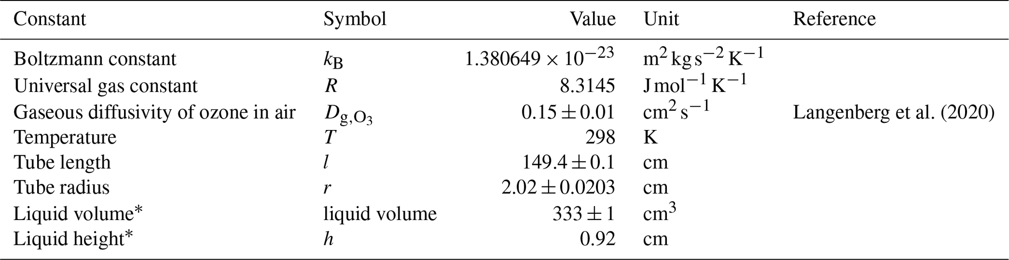
∗ Liquid volume in the flow reactor varied day to day; average values for liquid volume and resulting liquid height are provided here for illustrative purposes. However, the measured daily volumes were used in calculations.
Errors were propagated using the exact formula for the propagation of error (Eq. B1).
For Eqs. (B2) to (B7), definitions and values for physical constants can be found in Table A1.
Flow tube volume, VFT (Eq. B2), and associated error (Eq. B3) are calculated as follows:
Headspace volume, VH (Eq. B4), and associated error (Eq. B5) are calculated as follows:
Surface area of liquid, SA (Eq. B6), and associated error (Eq. B7) are calculated as follows:
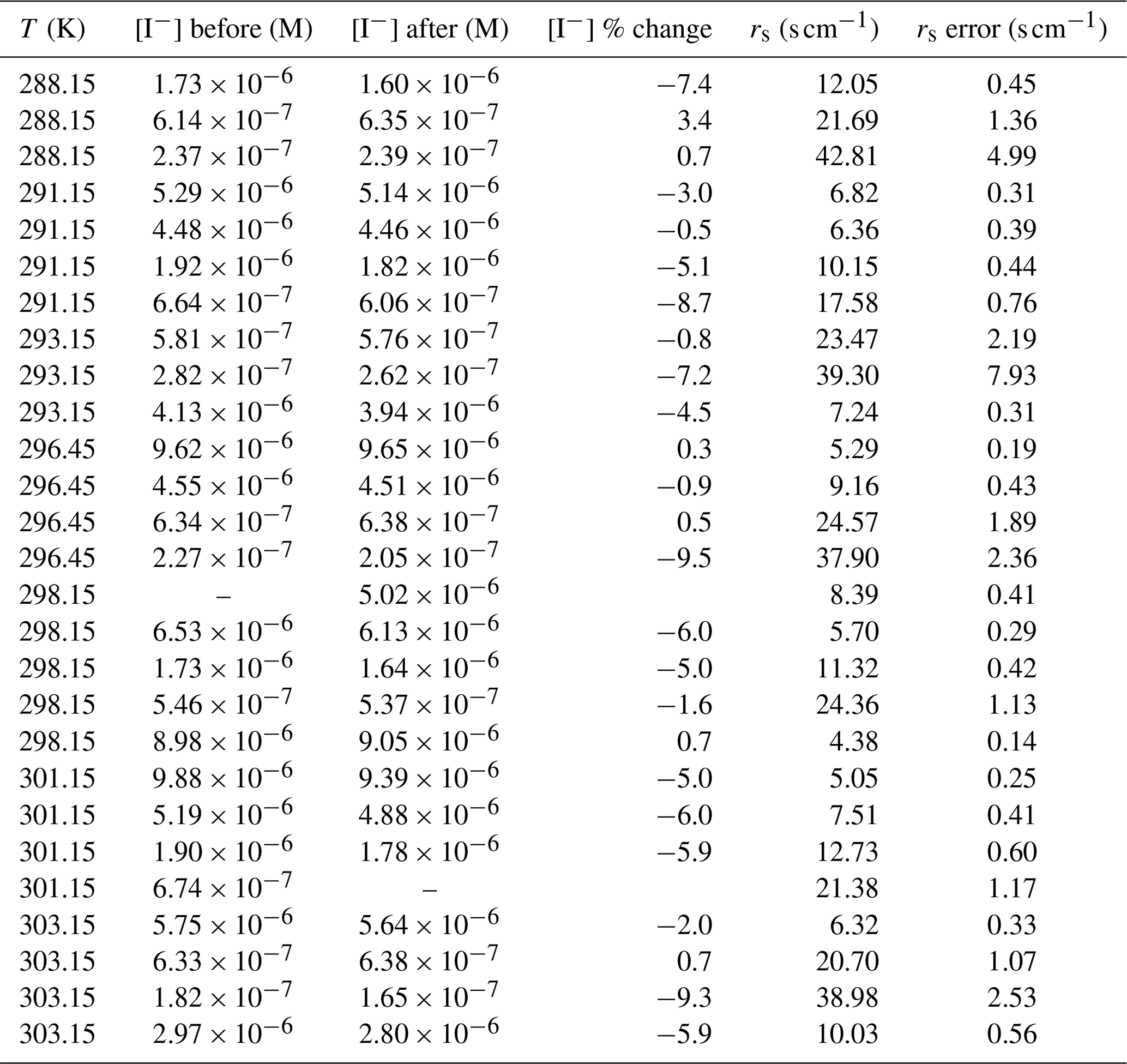
Iodide concentrations before and after passing through the flow tube and calculated rs at each iodide concentration and temperature are outlined in Table C1.
Table C1Iodide concentrations before and after passing through the flow reactor and associated rs measurements. The symbol – denotes that the measurement is not available.
This model was developed for the prediction of ozone deposition to the SML and the calculation of subsequent emission of halogenated species. It was designed for environmental conditions; however, it has been adapted and applied to lab experiments over iodide solutions for the purpose of this work. This model was developed in Python using Cantera as the chemistry solver (Goodwin et al., 2022). The model presented here also uses functions from SciPy (Virtanen et al., 2020), pandas (pandas development team, 2020) and NumPy (Harris et al., 2020). A summary of the model is included below, but for a complete description and characterisation of the model, see Pound et al. (2023).
In the model, ozone dry deposition velocity (vd) is calculated using the resistance-in-series scheme (Wesely and Hicks, 1977), which calculates the flux of ozone into the ocean surface microlayer. Air-side resistances that represent turbulent transport to the surface and transport through the quasi-laminar sub-layer, which is the air directly in contact with the surface microlayer, are calculated from wind speed, friction velocity and the Schmidt number of ozone in air (Chang et al., 2004). The surface resistance (rs) is calculated using the two-layer method of Luhar et al. (2018) from the dimensionless solubility, the chemical reactivity, the diffusivity in water, the waterside friction velocity, the thickness of the reaction–diffusion layer of the sea surface microlayer, and the modified Bessel functions of the second kind of zeroth and first order. Dry deposition velocity vd is coupled with the SML chemistry via I− concentration and is recalculated as the model advances towards equilibrium.
This model focuses on the aqueous inorganic halogen chemistry in the SML, applying an extended set of inorganic iodine chemistry compared to that described by Carpenter et al. (2013). The rate constant used for the reaction between ozone and iodide is that which was calculated in this work. The net flux of I2 and HOI into the atmosphere is calculated from the concentration in the liquid surface and the concentration in the atmosphere, along with the dimensionless Henry's law coefficient for each species, friction velocity, drag coefficient, Schmidt number and von Kármán constant.
This model accounts for mixing from the surface into underlying solution and follows the form of approach used by Cen-Lin and Tzung-May (2013). The first of these (molecular transfer) is calculated from the waterside transfer velocity and the bulk and surface concentrations of the species in question. In this model, there is the facility to account for the effects of surfactants; however, we expect no surfactant effect in this work, so this was turned off. The second process, mixing from surface renewal, is a significantly slower process than the mixing described above and is typically on the order of several minutes but has been included for completeness.
Conditions were chosen to mimic the experiments described by MacDonald et al. (2014). The model is “buffered” to pH 8 by manually resetting H+ and OH− at each time step to maintain a constant pH. For the ozone mixing ratio and iodide concentrations a range of values were reported, and the implications of this are discussed in Sect. 3.2.
Underlying code to run the sea-surface microlayer model can be accessed through Pound et al. (2023).
For the kinetic analysis, the data supporting this research are available for download from the research data repository of the University of York at https://doi.org/10.15124/38456dc5-1cf8-42be-bcb2-f7b348f645e8 (Pound et al., 2024).
Data for the sea-surface microlayer model can be accessed through Pound et al. (2023).
LVB carried out laboratory work, analysed model output and prepared the paper. RJP carried out modelling work. LSE assisted with laboratory work. MRJ carried out iodide quantification. SJA and LVB developed the laboratory method. LJC oversaw laboratory and modelling work and paper preparation.
The contact author has declared that none of the authors has any competing interests.
Publisher's note: Copernicus Publications remains neutral with regard to jurisdictional claims made in the text, published maps, institutional affiliations, or any other geographical representation in this paper. While Copernicus Publications makes every effort to include appropriate place names, the final responsibility lies with the authors.
The Viking cluster was used during this project, which is a high-performance computing facility provided by the University of York. We are grateful for computational support from the University of York, IT Services and the Research IT team. We would like to thank all three anonymous reviewers for their encouraging and constructive feedback. We appreciate their contribution to improving the quality of this paper.
This research has been supported by the European Research Council, Horizon Europe European Research Council (grant no. 833290).
This paper was edited by Markus Ammann and reviewed by three anonymous referees.
Campos, M. L. A., Farrenkopf, A. M., Jickells, T. D., and Luther, G. W.: A comparison of dissolved iodine cycling at the Bermuda Atlantic Time-series station and Hawaii Ocean Time-series station, Deep-Sea Res. Pt. II, 43, 455–466, https://doi.org/10.1016/0967-0645(95)00100-x, 1996. a
Campos, M. L. A., Sanders, R., and Jickells, T. D.: The dissolved iodate and iodide distribution in the South Atlantic from the Weddell Sea to Brazil, Mar. Chem., 65, 167–175, https://doi.org/10.1016/S0304-4203(98)00094-2, 1999. a
Carpenter, L. J., MacDonald, S. M., Shaw, M. D., Kumar, R., Saunders, R. W., Parthipan, R., Wilson, J., and Plane, J. M.: Atmospheric iodine levels influenced by sea surface emissions of inorganic iodine, Nat. Geosci., 6, 108–111, https://doi.org/10.1038/ngeo1687, 2013. a, b, c
Cen-Lin, H. and Tzung-May, F.: Air–Sea Exchange of Volatile Organic Compounds: A New Model with Microlayer Effects, Atmospheric and Oceanic Science Letters, 6, 97–102, https://doi.org/10.1080/16742834.2013.11447063, 2013. a
Chance, R. J., Baker, A. R., Carpenter, L. J., and Jickells, T. D.: The distribution of iodide at the sea surface, Environ. Sci.-Proc. Imp., 16, 1841–1859, https://doi.org/10.1039/c4em00139g, 2014. a, b, c
Chance, R. J., Tinel, L., Sherwen, T., Baker, A. R., Bell, T., Brindle, J., Campos, M. L. A., Croot, P., Ducklow, H., Peng, H., Hopkins, F., Hoogakker, B., Hughes, C., Jickells, T. D., Loades, D. C., Macaya, D. A. R., Mahajan, A. S., Malin, G., Phillips, D., Roberts, I., Roy, R., Sarkar, A., Sinha, A. K., Song, X., Winkelbauer, H., Wuttig, K., Yang, M., Peng, Z., and Carpenter, L. J.: Global sea-surface iodide observations, 1967–2018, Scientific Data, 6, 1–8, https://doi.org/10.1038/s41597-019-0288-y, 2019. a
Chang, W., Heikies, B. G., and Lee, M.: Ozone deposition to the sea surface: chemical enhancement and wind speed dependence, Atmos. Environ., 38, 1053–1059, 2004. a, b
Clifford, D., Donaldson, D. J., Brigante, M., D'Anna, B., and George, C.: Reactive uptake of ozone by chlorophyll at aqueous surfaces, Environ. Sci. Technol., 42, 1138–1143, https://doi.org/10.1021/es0718220, 2008. a
Coleman, L., Varghese, S., Tripathi, O. P., Jennings, S. G., and O'Dowd, C. D.: Regional-Scale Ozone Deposition to North-East Atlantic Waters, Adv. Meteorol., 2010, 1–16, https://doi.org/10.1155/2010/243701, 2010. a
Davidovits, P., Kolb, C. E., Williams, L. R., Jayne, J. T., and Worsnop, D. R.: Mass accommodation and chemical reactions at gas-liquid interfaces, Chem. Rev., 106, 1323–1354, https://doi.org/10.1021/cr040366k, 2006. a
De Souza, F. P. and Sen Gupta, R.: Fluoride, bromide and iodide in the southwestern Indian Ocean sector of the Southern Ocean, Deep Sea Research Part B. Oceanographic Literature Review, 31, 856, https://doi.org/10.1016/0198-0254(84)93266-7, 1984. a
Donaldson, D. J., Mmereki, B. T., Chaudhuri, S. R., Handley, S., and Oh, M.: Uptake and reaction of atmospheric organic vapours on organic films, Faraday Discuss., 130, 227–239, https://doi.org/10.1039/b418859d, 2005. a
Forster, P., Ramaswamy, V., Artaxo, P., Berntsen, T., Betts, R., Fahey, D., Haywood, J., Lean, J., Lowe, D., Myhre, G., Nganga, J., Prinn, R., Raga, G., Schulz, M., and Dorland, R. V.: Changes in Atmospheric Constituents and in Radiative Forcing, in: Climate Change 2007: The Physical Science Basis. Contribution of Working Group I to the Fourth Assessment Report of the Intergovernmental Panel on Climate Change, Cambridge University Press, Cambridge, United Kingdom and New York, NY, USA, https://doi.org/10.20892/j.issn.2095-3941.2017.0150, 2007. a
Galbally, I. E. and Roy, C. R.: Destruction of ozone at the earth's surface, Q. J. Roy. Meteor. Soc., 106, 599–620, 1980. a, b
Gallagher, M. W., Beswick, K. M., and Coe, H.: Ozone deposition to coastal waters, Q. J. Roy. Meteor. Soc., 127, 539–558, 2001. a
Gálvez, Ó., Teresa Baeza-Romero, M., Sanz, M., and Pacios, L. F.: A theoretical study on the reaction of ozone with aqueous iodide, Phys. Chem. Chem. Phys., 18, 7651–7660, https://doi.org/10.1039/c5cp06440f, 2016. a
Ganzeveld, L., Helmig, D., Fairall, C., Hare, J. E., and Pozzer, A.: Atmosphere-ocean ozone exchange: A global modeling study of biogeochemical, atmospheric, and waterside turbulence dependencies, Global Biogeoch. Cy., 23, 1–16, https://doi.org/10.1029/2008GB003301, 2009. a, b, c
Garland, J. A., Elzerman, A. W., and Penkett, S.: The Mechanism for Dry Deposition of Ozone to Seawater Surfaces, J. Geophys. Res., 85, 7488–7492, 1980. a, b, c, d, e, f, g
Goodwin, D. G., Moffat, H. K., Schoegl, I., Speth, R. L., and Weber, B. W.: Cantera: An Object-oriented Software Toolkit for Chemical Kinetics, Thermodynamics, and Transport Processes, https://www.cantera.org (last access: 27 March 2024), 2022. a
Hardacre, C., Wild, O., and Emberson, L.: An evaluation of ozone dry deposition in global scale chemistry climate models, Atmos. Chem. Phys., 15, 6419–6436, https://doi.org/10.5194/acp-15-6419-2015, 2015. a
Harris, C. R., Millman, K. J., van der Walt, S. J., Gommers, R., Virtanen, P., Cournapeau, D., Wieser, E., Taylor, J., Berg, S., Smith, N. J., Kern, R., Picus, M., Hoyer, S., van Kerkwijk, M. H., Brett, M., Haldane, A., del Río, J. F., Wiebe, M., Peterson, P., Gérard-Marchant, P., Sheppard, K., Reddy, T., Weckesser, W., Abbasi, H., Gohlke, C., and Oliphant, T. E.: Array programming with NumPy, Nature, 585, 357–362, https://doi.org/10.1038/s41586-020-2649-2, 2020. a
Heikies, B. G., Lee, M., Jacob, D., Talbot, R., Bradshaw, J., Singh, H., Blake, D., Anderson, B., Fuelberg, H., and Thompson, A. M.: Ozone , hydroperoxides , oxides of nitrogen , and hydrocarbon budgets in the marine boundary layer over the South Atlantic, J. Geophys. Res., 101, 24221–24234, 1996. a
Helmig, D., Boylan, P., Johnson, B., Oltmans, S., Fairall, C., Staebler, R., Weinheimer, A., Orlando, J., Knapp, D. J., Montzka, D. D., Flocke, F., Frieó, U., Sihler, H., and Shepson, P. B.: Ozone dynamics and snow-atmosphere exchanges during ozone depletion events at Barrow, Alaska, J. Geophys. Res.-Atmos., 117, 1–15, https://doi.org/10.1029/2012JD017531, 2012. a
Hu, J. H., Shi, Q., Davidovits, P., Worsnop, D. R., Zahniser, M. S., and Kolb, C. E.: Reactive uptake of Cl2(g) and Br2(g) by aqueous surfaces as a function of Br− and I− ion concentration. The effect of chemical reaction at the interface, J. Phys. Chem., 99, 8768–8776, https://doi.org/10.1021/j100021a050, 1995. a, b, c, d
Johnson, M. T.: A numerical scheme to calculate temperature and salinity dependent air-water transfer velocities for any gas, Ocean Sci., 6, 913–932, https://doi.org/10.5194/os-6-913-2010, 2010. a, b
Johnson, P. N. and Davis, R. A.: Diffusivity of ozone in water, J. Chem. Eng. Data, 41, 1485–1487, https://doi.org/10.1021/je9602125, 1996. a
Jones, M. R., Chance, R. J., Dadic, R., Hannula, H. R., May, R., Ward, M., and Carpenter, L. J.: Environmental iodine speciation quantification in seawater and snow using ion exchange chromatography and UV spectrophotometric detection, Anal. Chim. Acta, 1239, 340700, https://doi.org/10.1016/j.aca.2022.340700, 2023. a
Kawa, S. R. and Pearson Jr., R.: Ozone Budgets From the Dynamics and Chemistry of Marine Stratocumulus Experiment, J. Geophys. Res., 94, 9809–9817, 1989. a, b
Koenig, T. K., Baidar, S., Campuzano-Jost, P., Cuevas, C. A., Dix, B., Fernandez, R. P., Guo, H., Hall, S. R., Kinnison, D., Nault, B. A., Ullmann, K., Jimenez, J. L., Saiz-Lopez, A., and Volkamer, R.: Quantitative detection of iodine in the stratosphere, P. Natl. Acad. Sci. USA, 117, 1860–1866, https://doi.org/10.1073/pnas.1916828117, 2020. a, b
Kosak-Channing, L. F. and Helz, G. R.: Solubility of Ozone in Aqueous Solutions of 0–0.6 M Ionic Strength at 5–30 °C, Tech. Rep. 2, University of Maryland, https://doi.org/10.1021/es00109a005, 1983. a
Langenberg, S., Carstens, T., Hupperich, D., Schweighoefer, S., and Schurath, U.: Technical note: Determination of binary gas-phase diffusion coefficients of unstable and adsorbing atmospheric trace gases at low temperature – arrested flow and twin tube method, Atmos. Chem. Phys., 20, 3669–3682, https://doi.org/10.5194/acp-20-3669-2020, 2020. a
Lenschow, D. H., Pearson Jr., R., and Boba Stankov, B.: Measurement of Ozone Vertical Flux to Ocean and Forest, J. Geophys. Res., 87, 8833–8837, 1982. a, b
Liu, Q., Schurter, L. M., Muller, C. E., Aloisio, S., Francisco, J. S., and Margerum, D. W.: Kinetics and mechanisms of aqueous ozone reactions with bromide, sulfite, hydrogen sulfite, iodide, and nitrite ions, Inorg. Chem., 40, 4436–4442, https://doi.org/10.1021/ic000919j, 2001. a, b, c, d, e, f, g
Luhar, A. K., Woodhouse, M. T., and Galbally, I. E.: A revised global ozone dry deposition estimate based on a new two-layer parameterisation for air–sea exchange and the multi-year MACC composition reanalysis, Atmos. Chem. Phys., 18, 4329–4348, https://doi.org/10.5194/acp-18-4329-2018, 2018. a
MacDonald, S. M., Gómez Martín, J. C., Chance, R., Warriner, S., Saiz-Lopez, A., Carpenter, L. J., and Plane, J. M. C.: A laboratory characterisation of inorganic iodine emissions from the sea surface: dependence on oceanic variables and parameterisation for global modelling, Atmos. Chem. Phys., 14, 5841–5852, https://doi.org/10.5194/acp-14-5841-2014, 2014. a, b, c, d, e, f, g, h, i, j
Magi, L., Schweitzer, F., Pallares, C., Cherif, S., Mirabel, P., and George, C.: Investigation of the uptake rate of ozone and methyl hydroperoxide by water surfaces, J. Phys. Chem. A, 101, 4943–4949, https://doi.org/10.1021/jp970646m, 1997. a, b, c, d, e, f, g
McKay, W. A., Stephens, B. A., and Dollard, G. J.: Laboratory measurements of ozone deposition to sea water and other saline solutions, Atmos. Environ. A-Gen., 26, 3105–3110, https://doi.org/10.1016/0960-1686(92)90467-Y, 1992. a
McVeigh, P., O'Dowd, C., and Berresheim, H.: Eddy Correlation Measurements of Ozone Fluxes over Coastal Waters West of Ireland, Adv. Meteorol., 2010, 1–7, https://doi.org/10.1155/2010/754941, 2010. a
Mmereki, B. T. and Donaldson, D. J.: Direct Observation of the Kinetics of an Atmospherically Important Reaction at the Air–Aqueous Interface, J. Phys. Chem. A, 107, 11038–11042, https://doi.org/10.1021/jp036119m, 2003. a
Mmereki, B. T., Donaldson, D. J., Gilman, J. B., Eliason, T. L., and Vaida, V.: Kinetics and products of the reaction of gas-phase ozone with anthracene adsorbed at the air–aqueous interface, Atmos. Environ., 38, 6091–6103, https://doi.org/10.1016/j.atmosenv.2004.08.014, 2004. a
Moreno, C. G. and Baeza-Romero, M. T.: A kinetic model for ozone uptake by solutions and aqueous particles containing I− and Br−, including seawater and sea-salt aerosol, Phys. Chem. Chem. Phys., 21, 19835–19856, https://doi.org/10.1039/c9cp03430g, 2019. a
Moreno, C. G., Gálvez, O., López-Arza Moreno, V., Espildora-García, E. M., and Baeza-Romero, M. T.: A revisit of the interaction of gaseous ozone with aqueous iodide. Estimating the contributions of the surface and bulk reactions, Phys. Chem. Chem. Phys., 20, 27571–27584, https://doi.org/10.1039/c8cp04394a, 2018. a, b, c
Myhre, G., Shindell, D., Bréon, F.-M., Collins, W., Fuglestvedt, J., Huang, J., Koch, D., Lamarque, J.-F., Lee, D., Mendoza, B., Nakajima, T., Robock, A., Stephens, G., Takemura, T., and Zhang, H.: Anthropogenic and Natural Radiative Forcing, in: Climate Change 2013: The Physical Science Basis. Contribution of Working Group I to the Fifth Assessment Report of the Intergovernmental Panel on Climate Change, vol. 9781107057, Cambridge University Press, Cambridge, United Kingdom and New York, NY, USA, https://doi.org/10.1017/CBO9781107415324.018, 2013. a
Nuvolone, D.: The effects of ozone on human health, Environ. Sci. Pollut. R., 25, 8074–8088, https://doi.org/10.1007/s11356-017-9239-3, 2018. a
Oh, I.-B., Byun, D. W., Kim, H.-C., Kim, S., and Cameron, B.: Modeling the effect of iodide distribution on ozone deposition to seawater surface, Atmos. Environ., 42, 4453–4466, https://doi.org/10.1016/j.atmosenv.2008.02.022, 2008. a
Pound, R. J., Brown, L. V., Evans, M. J., and Carpenter, L. J.: An improved estimate of inorganic iodine emissions from the ocean using a coupled surface microlayer box model, EGUsphere [preprint], https://doi.org/10.5194/egusphere-2023-2447, 2023. a, b, c, d, e, f, g, h, i, j
Pound, R., Carpenter, L. J., and Brown, L.: Supporting Data for temperature dependence, University of York, LVB_supporting_data(.zip) [data set], https://doi.org/10.15124/38456dc5-1cf8-42be-bcb2-f7b348f645e8, 2024. a
Rai, R. and Agrawal, M.: Impact of tropospheric ozone on crop plants, P. Natl. A. Sci. India B, 82, 241–257, https://doi.org/10.1007/s40011-012-0032-2, 2012. a
Raja, S. and Valsaraj, K. T.: Heterogeneous oxidation by ozone of naphthalene adsorbed at the air-water interface of micron-size water droplets, J. Air Waste Manage., 55, 1345–1355, https://doi.org/10.1080/10473289.2005.10464732, 2005. a
Ramaswamy, V., Boucher, O., Haigh, J., Hauglustaine, D., Haywood, J., Myhre, G., Nakajima, T., Shi, G., and Solomon, S.: Radiative forcing of climate change, in: Climate Change 2001: The Scientific Basis. Contribution of Working Group I to the Third Assessment Report of the Intergovernmental Panel on Climate Change, vol. 94, Cambridge University Press, Cambridge, United Kingdom and New York, NY, USA, https://doi.org/10.1023/A:1026752230256, 2001. a
Read, K. A., Mahajan, A. S., Carpenter, L. J., Evans, M. J., Faria, B. V., Heard, D. E., Hopkins, J. R., Lee, J. D., Moller, S. J., Lewis, A. C., Mendes, L., McQuaid, J. B., Oetjen, H., Saiz-Lopez, A., Pilling, M. J., and Plane, J. M.: Extensive halogen-mediated ozone destruction over the tropical Atlantic Ocean, Nature, 453, 1232–1235, https://doi.org/10.1038/nature07035, 2008. a
Rouvière, A., Sosedova, Y., and Ammann, M.: Uptake of ozone to deliquesced KI and mixed KI/NaCl aerosol particles, J. Phys. Chem. A, 114, 7085–7093, https://doi.org/10.1021/jp103257d, 2010. a, b, c
Saiz-Lopez, A. and Von Glasow, R.: Reactive halogen chemistry in the troposphere, Chem. Soc. Rev., 41, 6448–6472, https://doi.org/10.1039/c2cs35208g, 2012. a
Sakamoto, Y., Yabushita, A., Kawasaki, M., and Enami, S.: Direct emission of I 2 molecule and IO radical from the heterogeneous reactions of gaseous ozone with aqueous potassium iodide solution, J. Phys. Chem. A, 113, 7707–7713, https://doi.org/10.1021/jp903486u, 2009. a
Sarwar, G., Kang, D., Foley, K., Schwede, D., Gantt, B., and Mathur, R.: Technical note: Examining ozone deposition over seawater, Atmos. Environ., 141, 255–262, https://doi.org/10.1016/j.atmosenv.2016.06.072, 2016. a, b
Schneider, S. R., Lakey, P. S. J., Shiraiwa, M., and Abbatt, J. P.: Reactive Uptake of Ozone to Simulated Seawater: Evidence for Iodide Depletion, J. Phys. Chem. A, 124, 9844–9853, https://doi.org/10.1021/acs.jpca.0c08917, 2020. a, b
Schneider, S. R., Lakey, P. S., Shiraiwa, M., and Abbatt, J. P.: Iodine emission from the reactive uptake of ozone to simulated seawater, Environ. Sci.-Proc. Imp., 25, 254–263, https://doi.org/10.1039/d2em00111j, 2022. a
Shaw, M. D. and Carpenter, L. J.: Modification of ozone deposition and I2 emissions at the air–aqueous interface by dissolved organic carbon of marine origin, Environ. Sci. Technol., 47, 10947–10954, https://doi.org/10.1021/es4011459, 2013. a, b, c, d, e
Sherwen, T., Chance, R. J., Tinel, L., Ellis, D., Evans, M. J., and Carpenter, L. J.: A machine-learning-based global sea-surface iodide distribution, Earth Syst. Sci. Data, 11, 1239–1262, https://doi.org/10.5194/essd-11-1239-2019, 2019. a
Stevenson, D. S., Dentener, F. J., Schultz, M. G., Ellingsen, K., van Noije, T. P., Wild, O., Zeng, G., Ammann, M., Atherton, C. S., Bell, N., Bergmann, D. J., Bey, I., Butler, T., Cofala, J., Collins, W. J., Derwent, R. G., Doherty, R. M., Drevet, J., Eskes, H. J., Fiore, A. M., Gauss, M., Hauglustaine, D. A., Horowitz, L. W., Isaksen, I. S., Krol, M. C., Lamarque, J. F., Lawrence, M. G., Montanaro, V., Müller, J. F., Pitari, G., Prather, M. J., Pyle, J. A., Rast, S., Rodriquez, J. M., Sanderson, M. G., Savage, N. H., Shindell, D. T., Strahan, S. E., Sudo, K., and Szopa, S.: Multimodel ensemble simulations of present-day and near-future tropospheric ozone, J. Geophys. Res.-Atmos., 111, D08301, https://doi.org/10.1029/2005JD006338, 2006. a
Stolle, C., Ribas-Ribas, M., Badewien, T. H., Barnes, J., Carpenter, L. J., Chance, R. J., Damgaard, L. R., María, A., Quesada, D., Engel, A., Frka, S., Galgani, L., Gašparović, B., Gerriets, M., Ili, N., Mustaffa, H., Herrmann, H., Kallajoki, L., Pereira, R., Radach, F., Revsbech, N. P., Rickard, P., Saint, A., Salter, M., Striebel, M., Triesch, N., Uher, G., Upstill-G, Oddard, R. C., Pinxteren, M. V., Zäncker, B., Zieger, P., and Wurl, O.: The MILAN Campaign: Studying Diel Light Effects on the Air–Sea Interface, B. Am. Meteorol. Soc., 101, 146–166, 2020. a
Teiwes, R., Elm, J., Handrup, K., Jensen, E. P., Bilde, M., and Pedersen, H. B.: Atmospheric chemistry of iodine anions: Elementary reactions of I−, IO−, and with ozone studied in the gas-phase at 300 K using an ion trap, Phys. Chem. Chem. Phys., 20, 28606–28615, https://doi.org/10.1039/c8cp05721d, 2018. a
Thompson, A. M. and Zafiriou, O. C.: Air–sea fluxes of transient atmospheric species, J. Geophys. Res.-Oceans, 88, 6696–6708, 1983. a, b
Virtanen, P., Gommers, R., Oliphant, T. E., Haberland, M., Reddy, T., Cournapeau, D., Burovski, E., Peterson, P., Weckesser, W., Bright, J., van der Walt, S. J., Brett, M., Wilson, J., Millman, K. J., Mayorov, N., Nelson, A. R., Jones, E., Kern, R., Larson, E., Carey, C. J., Polat, I., Feng, Y., Moore, E. W., VanderPlas, J., Laxalde, D., Perktold, J., Cimrman, R., Henriksen, I., Quintero, E. A., Harris, C. R., Archibald, A. M., Ribeiro, A. H., Pedregosa, F., van Mulbregt, P., Vijaykumar, A., Bardelli, A. P., Rothberg, A., Hilboll, A., Kloeckner, A., Scopatz, A., Lee, A., Rokem, A., Woods, C. N., Fulton, C., Masson, C., Häggström, C., Fitzgerald, C., Nicholson, D. A., Hagen, D. R., Pasechnik, D. V., Olivetti, E., Martin, E., Wieser, E., Silva, F., Lenders, F., Wilhelm, F., Young, G., Price, G. A., Ingold, G. L., Allen, G. E., Lee, G. R., Audren, H., Probst, I., Dietrich, J. P., Silterra, J., Webber, J. T., Slavič, J., Nothman, J., Buchner, J., Kulick, J., Schönberger, J. L., de Miranda Cardoso, J. V., Reimer, J., Harrington, J., Rodríguez, J. L. C., Nunez-Iglesias, J., Kuczynski, J., Tritz, K., Thoma, M., Newville, M., Kümmerer, M., Bolingbroke, M., Tartre, M., Pak, M., Smith, N. J., Nowaczyk, N., Shebanov, N., Pavlyk, O., Brodtkorb, P. A., Lee, P., McGibbon, R. T., Feldbauer, R., Lewis, S., Tygier, S., Sievert, S., Vigna, S., Peterson, S., More, S., Pudlik, T., Oshima, T., Pingel, T. J., Robitaille, T. P., Spura, T., Jones, T. R., Cera, T., Leslie, T., Zito, T., Krauss, T., Upadhyay, U., Halchenko, Y. O., and Vázquez-Baeza, Y.: SciPy 1.0: fundamental algorithms for scientific computing in Python, Nat. Methods, 17, 261–272, https://doi.org/10.1038/s41592-019-0686-2, 2020. a
von Sonntag, C. and von Gunten, U.: Chemistry of Ozone in Water and Wastewater Treatment: From Basic Principles to Applications, IWA Publishing, London, https://doi.org/10.2166/9781780400839, 2015. a
Watson, R. T., Zinyowera, M., Moss, R., Moreno, R. A., Adhikary, S., Adler, M., Agrawala, S., Aguilar, A. G., Al-Khouli, S., Allen-Diaz, B., Ando, M., Andressen, R., Ang, B., Arnell, N., Arquit-Niederberger, A., Baethgen, W., Bates, B., Beniston, M., Bierbaum, R., Bijlsma, L., Boko, M., Bolin, B., Bolton, S., Bravo, E., Brown, S., Bullock, P., Cannell, M., Canziani, O., Carcavallo, R., Cerri, C. C., Chandler, W., Cheghe, F., Liu, C., Cole, V., Cramer, W., Cruz, R., Davidson, O., Desa, E., Xu, D., Diaz, S., Dlugoleck, A., Edmonds, J., Everett, J., Fischlin, A., Fitzharris, B., Fox, D., Friaa, J., Gacuhi, A. R., Galinski, W., Gitay, H., Groffman, P., Grubler, A., Gruenspecht, H., Hamburg, S., Hoffman, T., Holten, J., Ishitani, H., Ittekkot, V., Johansson, T., Kaczmarek, Z., Kashiwagi, T., Kirschbaum, M., Komor, P., Krovnin, A., Klein, R., Kulshrestha, S., H. Lang, S., Houerou, L., Leemans, R., Levine, M., Erda, L., Lluch-Belda, D., MacCracken, M., Magnuson, J., Mailu, G., Maitima, J. M., Marland, G., Maskell, K., McLean, R., McMichael, A., Michaelis, L., Miles, E., Moomaw, W., Moreira, R., Mulholland, P., Nakicenovic, N., Nicholls, R., Nishioka, S., Noble, I., Nurse, L., Odongo, R., Ohashi, R., Okemwa, E., Oquist, M., Parry, M., Perdomo, M., Petit, M., Piver, W., Ramakrishnan, P., Ravindranath, N., Reilly, J., Riedacker, A., Rogner, H.-H., Sathaye, J., Sauerbeck, D., Scott, M., Sharma, S., Shriner, D., Sinha, S., Skea, J., Solomon, A., Stakhiv, E., Starosolszky, O., Jilan, S., Suarez, A., Svensson, B., Takakura, H., Taylor, M., L.Tessier, Tirpak, D., Lien, T. V., Troadec, J.-P., Tsukamoto, H., Tsuzaka, I., Vellinga, P., Williams, T., Young, P., Xie, Y., and Fengqi, Z.: IPCC 1995: Second Assessment: Climate Change, Tech. Rep. 8, IPCC, https://archive.ipcc.ch/pdf/climate-changes-1995/ipcc-2nd-assessment/2nd-assessment-en.pdf (last access: 27 March 2024), 1995. a
Wesely, M. L. and Hicks, B. B.: Some factors that affect the deposition rates of sulfur dioxide and similar gases on vegetation, JAPCA J. Air Waste Ma., 27, 1110–1116, https://doi.org/10.1080/00022470.1977.10470534, 1977. a
Wesely, M. L. and Hicks, B. B.: A review of the current status of knowledge on dry deposition, Atmos. Environ., 34, 2261–2282, 2000. a
Wesely, M. L., Cook, D. R., and Williams, R. M.: Field Measurement of Small Ozone Fluxes to Snow, Wet Bare Soil, and Lake Water, Bound.-Lay. Meteorol., 20, 459–471, 1981. a
Whitehead, J. D., Mcfiggans, G. B., Gallagher, M. W., and Flynn, M. J.: Direct linkage between tidally driven coastal ozone deposition fluxes, particle emission fluxes, and subsequent CCN formation, Geophys. Res. Lett., 36, 1–5, https://doi.org/10.1029/2008GL035969, 2009. a
Zhou, S., Gonzalez, L., Leithead, A., Finewax, Z., Thalman, R., Vlasenko, A., Vagle, S., Miller, L. A., Li, S.-M., Bureekul, S., Furutani, H., Uematsu, M., Volkamer, R., and Abbatt, J.: Formation of gas-phase carbonyls from heterogeneous oxidation of polyunsaturated fatty acids at the air–water interface and of the sea surface microlayer, Atmos. Chem. Phys., 14, 1371–1384, https://doi.org/10.5194/acp-14-1371-2014, 2014. a
- Abstract
- Introduction
- Methods
- Results and discussion
- Conclusions
- Appendix A: Physical constants
- Appendix B: Geometric equations and error calculation
- Appendix C: Iodide concentrations measured by ion exchange chromatography (IC)
- Appendix D: Model description
- Code availability
- Data availability
- Author contributions
- Competing interests
- Disclaimer
- Acknowledgements
- Financial support
- Review statement
- References