Identification of stratospheric disturbance information in China based on the round-trip intelligent sounding system

Assessing the role of physical processes in the stratosphere under climate change has been one of the hottest topics over the past few decades. However, due to the limitations of detection techniques, stratospheric disturbance information from in situ observations is still relatively scarce. The round-trip intelligent sounding system (RTISS) is a new detection technology, developed in recent years, that can capture atmospheric fine-structure information about the troposphere and stratosphere via three-stage (rising, flat-floating, and falling) detection. Based on the structure function and singular measure relationships, we quantify stratospheric small-scale gravity waves (SGWs) over China, using the Hurst and intermittency parameters, and discuss their relationship with inertia-gravity waves (IGWs). The results show that the enhancement of SGWs in the stratosphere is accompanied by weakening of the IGWs below, which is related to the Kelvin–Helmholtz instability (KHI), and is conducive to the transport of ozone to higher altitudes from lower stratosphere. The parameter space (H1, C1) shows sufficient potential in the analysis of stratospheric disturbances and their role in material transport and energy transfer.

1 Introduction

Gravity waves (GWs) are waves generated by gravity and are widespread in the Earth's atmosphere. GWs are excited by wave sources in the troposphere, including topography, convection, and wind shear, and they propagate from the troposphere to the stratosphere and higher altitudes (Alexander et al., 2010; Fritts and Alexander, 2003, 2012). During the upward propagation of GWs, due to the decrease in atmospheric density and the increase in wave amplitudes (Fritts and Alexander, 2003; Mohankumar, 2008), the influence of GWs on the surrounding atmosphere is increasingly important. This effect is mainly caused by the instability of GWs with increasing amplitude or the breaking of GWs when they encounter the “critical layer”, thereby changing the circulation and structure of the atmosphere by dissipating energy and momentum (Allen and Vincent, 1995; Hertzog et al., 2012).

In order to improve the simulation of the main average characteristics of the atmosphere by numerical weather prediction (NWP) and general circulation models (GCMs), it is necessary to describe important physical processes in the atmosphere more accurately and efficiently (Kim et al., 2003). Part of the GWs have relatively small scales and cannot be resolved in models with a relatively rough resolution, so it is necessary to use a parameterization to describe the influence and interaction of GWs on larger-scale dynamic process. The GW parameterization is now a key component of almost all large-scale atmospheric models. However, due to the lack of observational constraints and an insufficient understanding of the mechanism, it also restricts the prediction accuracy and simulation ability of the models (Plougonven et al., 2020).

Assessing the role of stratospheric physical processes under climate change has been one of the hottest topics over the past few decades (SPARC, 2022; Tian et al., 2023). GWs, as one of the important physical processes in the stratosphere, have been extensively studied, based on radiosonde (Kinoshita et al., 2019; Moffat-Griffin et al., 2013), rocket (Eckermann et al., 1995), radar (Alexander et al., 2017; Huang et al., 2017), remote sensing (Wright et al., 2016; Guo et al., 2021), and other detection methods. Limited by the detection technology, relatively little research has been carried out on the fine structure of the stratospheric atmosphere. Aircraft observation can only be used for specific design tasks (Zhang et al., 2015), with little continuous data accumulation. Super-pressure balloons can provide stratospheric GW field information on particular zonal circles with long-duration observation (Alexander et al., 2021; Hertzog et al., 2008), although it is not currently applicable to local areas within countries.

At present, stratospheric disturbance information in the horizontal direction is still relatively scarce in China, and the introduction of flat-floating information can help to improve the forecasting effect of the models and deepen the understanding of stratospheric dynamic processes (Laroche and Sarrazin, 2013; Cohn et al., 2013). The round-trip intelligent sounding system (RTISS) is a new detection technology, developed in recent years (Cao et al., 2019), that can capture atmospheric fine-structure information about the troposphere and stratosphere via three-stage (rising, flat-floating, and falling) detection. That is, the outer balloon carries the radiosonde for ascending detection, the inner balloon continues to carry the radiosonde for stratospheric detection after the outer balloon explodes, and the radiosonde is carried by the parachute for descending detection after the flat-floating stage is over. For the first time, this paper shows a relatively complete analysis of atmospheric disturbance information in the horizontal direction of the stratosphere in China through RTISS and provides an innovative result for the evaluation of physical processes in the stratosphere.

2 Observation from RTISS

2.1 Introduction to experimental data

Data used in the paper are from an experimental project using the round-trip intelligent sounding system (RTISS) and cover sites in China, including the following: Yichang (YC), Wuhan (WH), Anqing (AQ), Changsha (CS), Nanchang (NC), and Ganzhou (GZ). The RTISS can realize three-stage detection, including the rising, flat-floating, and falling stages, and has become an important source of atmospheric disturbance information for analysis in the horizontal direction of the stratosphere (Cao et al., 2019; He et al., 2022). The release time span is from 1 June to 10 July (summer) and from 13 October to 18 November (autumn) in 2018. There are 245 detections in autumn (34 in AQ, 34 in GZ, 46 in NC, 43 in WH, 47 in YC, and 41 in CS) and 245 detections in summer (40 in AQ, 48 in GZ, 43 in NC, 44 in WH, 50 in YC, and 20 in CS).

The details of the observation experiment are shown in Fig. 1. The flat-floating height covers the range of 18–32 km and is mainly concentrated in the 26–30 km range (Fig. 1a); the variation in height over time during the entire detection process is shown in Fig. A1. Six sites are all located in southeast China (Fig. 1b). The balloon trajectories can directly reflect the stratospheric wind field characteristics over the corresponding sites (Fig. 1c, d, e, f, h). In summer, the stratosphere is mainly dominated by easterly winds, with relatively stable circulation (more consistent trajectories), whereas circulation changes more frequently (more divergent trajectories) in autumn.

In order to explore the correlation between RTISS data and atmospheric composition, we obtained ozone and potential vorticity from ERA5 reanalysis data (0.25° × 0.25°). The release time of flat-floating detection is divided into two periods: morning and evening. The release is done at approximately 23:00 UTC (07:00 CST, Beijing time) and 11:00 UTC (19:00 CST). Considering the rise time of nearly 1–1.5 h, the balloon begins the flat-floating stage at approximately 00:00 and 12:00 UTC for day and night detection, respectively. Therefore, the 00:00 and 12:00 UTC data provided by ERA5 can be well combined with the observation results of RTISS in the flat-floating stage for analysis.

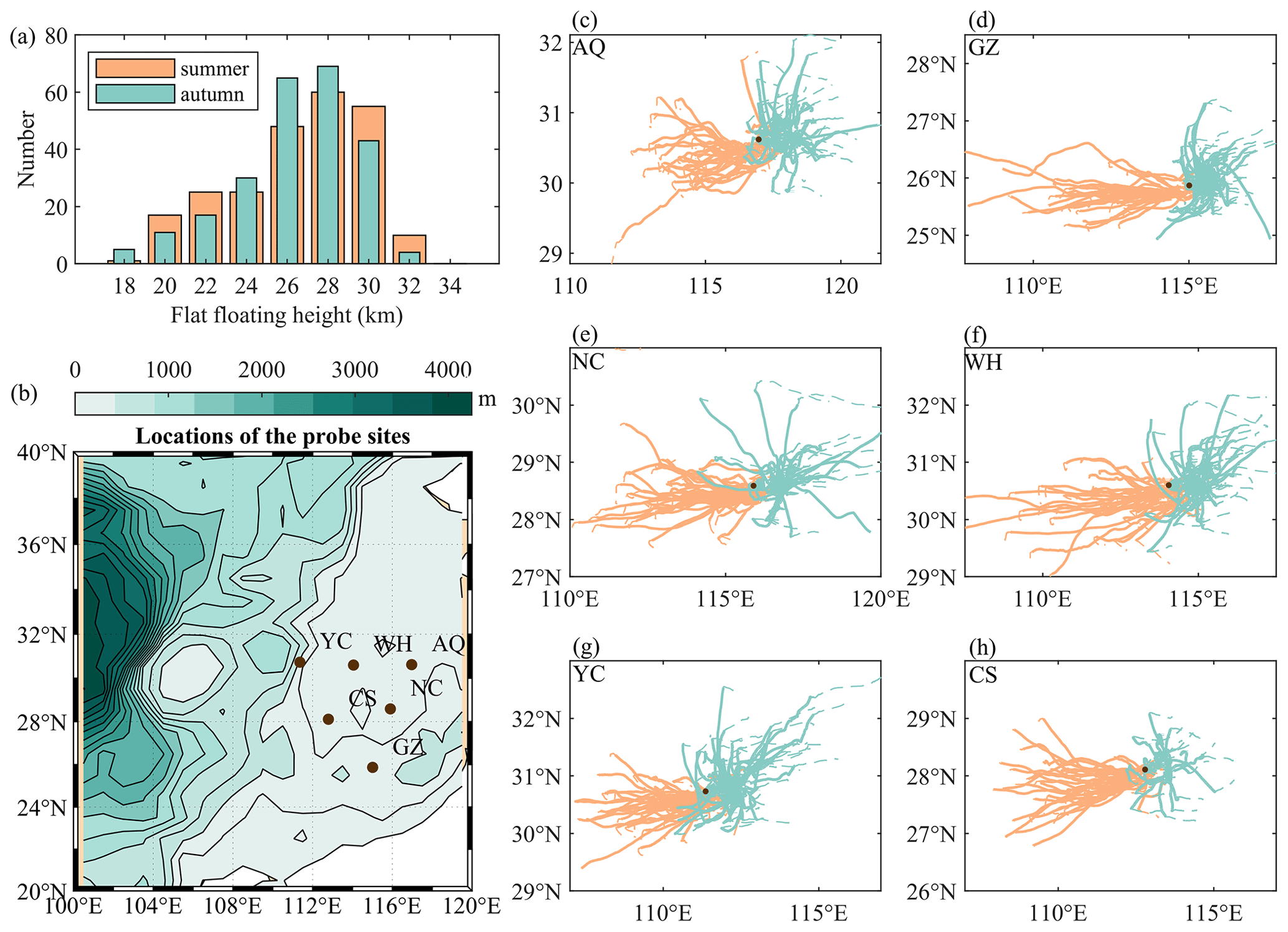
Figure 1 Panel (a) presents a histogram of the flat-floating height. Panel (b) shows a topographic map of the RTISS release sites and nearby areas. Panels (c), (d), (e), (f), (g), and (h) display the trajectories of RTISS over Anqing, Ganzhou, Nanchang, Wuhan, Yichang, and Changsha, respectively. The black dots represent the release sites, the dashed lines represent trajectories during the rising and falling stages, and the solid lines represent trajectories during the flat-floating stage. In order to better compare the results of different sites, the axes of panels (c)–(h) are unified to the same geographic width (10° × 4°).

2.2 The detection principle and quality control

RTISS aims to maintain a relatively low cost while achieving encrypted observations several hours apart in the vertical direction (several hours between the end of the detection in the rising stage and the beginning of the detection in the falling stage) as well as continuous high-frequency observations (1 s temporal resolution) for several hours at a specific altitude (flat-floating stage) in order to capture the atmospheric fine-structure information from the troposphere to the stratosphere, including the wind field, temperature, air pressure, and relative humidity (RH). The sounding instrument carries the BeiDou navigation system and a meteorological sensor. The BeiDou navigation system provides positioning information (longitude, latitude, and altitude) that can be used to calculate the horizontal wind field. The uncertainty in the wind speed is 2 m s⁻¹ during the rising stage and 4 m s⁻¹ during the flat-floating stage. The sensor module can be used to obtain temperature, RH, and air pressure, and it consists of three parts: (1) a negative temperature coefficient (NTC) thermistor sensor for temperature measurement that has an uncertainty of 0.8 K during rising stage and 2.8 K during flat-floating stage; (2) a piezoresistive sensor for air pressure measurement that has an uncertainty of 1 hPa during the rising stage and flat-floating stage; and (3) a humidity-sensitive capacitance sensor that has an uncertainty of 10 % RH during the rising stage but is ignored during flat-floating stage due to poor data quality. The uncontrolled, high-velocity descent via parachute during falling stage may influence the measurement quality due to a strong pendulum motion (Jorge et al., 2021); therefore, we do not consider the data from this stage.

The three-stage RTISS detection process is described in Fig. 2. During the rising stage, the two-balloon method (an inner balloon inside an outer balloon) is used to carry the radiosonde up and make real-time measurements. When a predetermined height is reached, the outer balloon is exploded; at that time, the buoyancy of the inner balloon is just equal to the gravity of the carried instrument, and it drifts with the wind at the predetermined height with a quasi-horizontal movement. Once the balloon floats for several hours to reach the predetermined area, the radiosonde and the inner balloon are separated by a fuse device; a parachute above the instrument then opens and the instrument descends.

Figure 2 The three-stage detection process by RTISS.

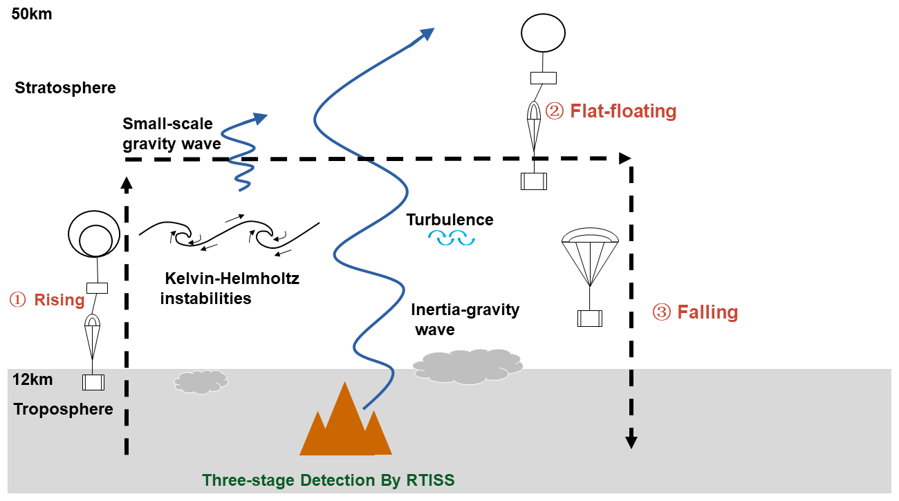
The detection system has different working principles during the three stages, and the specific dynamic process is outlined in previous work (Cao et al., 2019). It should be noted that the RTISS uses a zero-pressure balloon to meet the needs of low-cost business observations; this is different from a super-pressure balloon (Hertzog et al., 2008). For a zero-pressure balloon, the bottom exhaust pipe makes the pressure difference between the inside and outside of the balloon basically zero, and the flight time is short (several hours). For a super-pressure balloon, in contrast, the sphere is closed, the volume of the sphere is basically unchanged, and the flight time is longer (several weeks).

It is known that a balloon payload can have a pendulum motion (Kräuchi et al., 2016); thus, we have selected an appropriate smooth fitting interval to eliminate this effect. An integer multiple of the swing period is used as the smooth fitting interval, and the symmetry of the swing is used to compensate for the swing deviation. Using the average smoothed position coordinates, the first derivative is obtained by linear fitting to establish the speed, whereas the second derivative is obtained by quartic fitting to establish the acceleration. Wind speed and wind direction can then be obtained. It should be noted that different smoothing points may cause some difference in the quantization results of GWs. However, if all datasets are smoothed in the same way, the internal comparison will not be affected by this.

The variation in height during the whole RTISS process over time is shown in Fig. A1. In order to ensure the premise of an approximately constant height, we need to sift through all of the flat-floating data, and only datasets with a long enough flat-floating time (longer than 3–4 h) and relatively good flat-floating quality (the difference between the maximum and minimum height is within several hundred meters) are selected. It should be noted that, after the outer balloon bursts, the platform adjusts to its equilibrium level a few hundred meters below the burst altitude (Fig. A1); thus, the initial segment after the outer balloon bursts is also discarded. Along the measured points, the flat-floating distance is usually tens of kilometers to hundreds of kilometers (in the same height plane), and a fluctuation of several hundred meters in the vertical direction can still be approximated as quasi-horizontal movement. The original data are tested for horizontal consistency and subsequently re-interpolated to a uniform spatial interval after the outliers and missing values are removed.

3 Analysis method

3.1 Third-order structure function

In order to effectively identify the atmospheric disturbance information obtained by the RTISS, we consider combining the results from the rising and flat-floating stages for analysis, but the falling stage is not included due to the relatively poor data quality. We assume that the RTISS can capture the same weather system during the rising and flat-floating stages due to the continuous observation in space and time. The observation results in the horizontal and vertical directions can complement each other, which is currently impossible for other single observations.

We use the third-order structure function S₃(r) to identify GWs and turbulence. This method has previously been used for aircraft observation data (Cho and Lindborg, 2001). At the tail of the S₃(r) (turbulence subrange), the r slope represents the occurrence of turbulence, whereas at larger scales (GW subrange) of S₃(r), the r² and r³ slopes represent the unstable and stable GWs, respectively (Lu and Koch, 2008; He et al., 2022). The related calculation is as follows (Cho and Lindborg, 2001; Lindborg, 1999):

$$\begin{array}{}\text{(1)}& S_{\mathrm{3}}\left(r\right)=\langle {\left[{\mathit{\delta }}_{u_L}\left(r\right)\right]}^{\mathrm{3}}\rangle +\mathrm{2}\langle {\mathit{\delta }}_{u_L}\left(r\right){\left[{\mathit{\delta }}_{u_T}\left(r\right)\right]}^{\mathrm{2}}\rangle =-{\displaystyle \frac{\mathrm{4}}{\mathrm{3}}}Er.\end{array}$$

Here, 〈.〉 is the ensemble average, r is the separation distance, and E is the energy dissipation rate. The balloon trajectory during flat-floating stage is not a straight line, so we decompose it into the zonal and meridional directions and take the direction of the longer projection distance as the separation distance direction. Separation distance can be determined as $r=l\times {\mathrm{2}}^n$ for integers $n=\mathrm{0},\mathrm{1}$..., N, where l is the average step along the separation distance direction and N is limited by the maximum data length L (in the current data, N=13 or N=14). The directions parallel to and perpendicular to the separation distance are represented by L and T, respectively. The raw data are uniformly interpolated to the average step along the separation distance direction.

3.2 The Hurst index and intermittent parameter

Similar to Eq. (1), the multi-order structure function is defined as follows:

$$\begin{array}{}\text{(2)}& S_q\left(r\right)=\langle \left|u_L\right(x+r)-u_L(x){|}^q\rangle =\langle |{\mathit{\delta }}_{u_L}\left(r\right){|}^q\rangle ,\end{array}$$

where $\mathrm{0}\ll x\ll L-r$. It should be noted that Eq. (1) is used to identify the state of the GWs and the energy cascade direction, whereas Eq. (2) is used to calculate the subsequent disturbance parameters, consistent with previous studies (Lu and Koch, 2008; Marshak et al., 1997). Assuming that this process is scale-invariant and self-similar, S_q(r) can be scaled as follows (Lu and Koch, 2008):

$$\begin{array}{}\text{(3)}& S_q\left(r\right)=C_q{r}^{\mathit{\zeta }\left(q\right)},q\ge \mathrm{0},\end{array}$$

where C_q is a constant and ζ(q) is a function of order q. From this, we can define a monotone, non-increasing function (Marshak et al., 1997):

$$\begin{array}{}\text{(4)}& H\left(q\right)={\displaystyle \frac{\mathit{\zeta }\left(q\right)}{q}}.\end{array}$$

Here, we define H1=H(1) as the Hurst index, which can measure the roughness (nonstationarity) of the signal in data and results in a value of between 0 and 1 (Marshak et al., 1997). The larger the H1, the smoother the data sequence and the fewer the wave packets superimposed on it, and vice versa.

A statistical analysis technique called singularity measurement can be used to reflect the intermittency of the data sequence (Marshak et al., 1997); a non-negative normalized η-scale gradient field is defined by a second-order structure function (Lu and Koch, 2008):

$$\begin{array}{}\text{(5)}& \mathit{\epsilon }\left(\mathit{\eta };x\right)={\displaystyle \frac{{\left|\mathit{\delta }{u}_L(x,\mathit{\eta })\right|}^{\mathrm{2}}}{\langle \left|{\mathit{\delta }}_{u_L}\right(x,\mathit{\eta }){|}^{\mathrm{2}}\rangle }},\mathit{\eta }\le x\le L-r,\end{array}$$

where L is the maximum length of the data and η=4 l is 4 times the Nyquist wavelength. The measurements at different separation distances r can be expressed by the results of spatial averaging:

$$\begin{array}{}\text{(6)}& \mathit{\epsilon }\left(r;x\right)={\displaystyle \frac{\mathrm{1}}{r}}{\int }_x^{x+r}\mathit{\epsilon }\left(\mathit{\eta };x{}^{\prime }\right)\mathrm{d}x{}^{\prime },\mathit{\eta }\le x\le L-r.\end{array}$$

The self-similarity of fluctuations means that the q-order measurement is expressed as follows:

$$\begin{array}{}\text{(7)}& \langle \mathit{\epsilon }(r;x{)}^q\rangle =\langle \mathit{\epsilon }(r{)}^q\rangle \propto r^{-K\left(q\right)},q\ge \mathrm{0}.\end{array}$$

By linearly fitting the ε(r) curves of different orders q, the K(q) curve can be obtained. Then, the generalized dimension is introduced:

$$\begin{array}{}\text{(8)}& D\left(q\right)=\mathrm{1}-{\displaystyle \frac{K\left(q\right)}{q-\mathrm{1}}}.\end{array}$$

The intermittent nature of fluctuations can be expressed as follows:

$$\begin{array}{}\text{(9)}& C\mathrm{1}=\mathrm{1}-D\left(\mathrm{1}\right)=\mathrm{1}-\begin{array}{c}\text{lim}\\ q\to \mathrm{1}\end{array}D\left(q\right)=\begin{array}{c}\text{lim}\\ q\to \mathrm{1}\end{array}{\displaystyle \frac{K\left(q\right)}{q-\mathrm{1}}}=K{}^{\prime }\left(\mathrm{1}\right).\end{array}$$

Here, C1 is an intermittent parameter with a value between 0 and 1, reflecting the singularity of the fluctuation (Marshak et al., 1997). The larger the C1, the more intermittency in nonstationary data and the more singular the fluctuations. According to Eqs. (5) and (7), it can be seen that the premise of Eq. (9) here is that K(1) = 0 (Lu and Koch, 2008).

3.3 Inertia-gravity waves (IGWs) and the turbulence parameter

Based on the data from the rising stage, we use hodograph analysis to extract IGW parameters (Bai et al., 2016; Huang et al., 2018) with a height interval of 18–25 km, thereby obtaining parameters including the vertical wavelength, horizontal wavelength, intrinsic frequency, propagation direction (anticlockwise from the y axis), kinetic energy, potential energy, and momentum flux. In order to eliminate the error caused by the random movement of the balloon, the data are uniformly interpolated to an interval of 50 m. The total energy is the sum of kinetic energy and potential energy.

Based on Thorpe analysis (Ko and Chun, 2022; Thorpe, 1977; Wilson et al., 2011), the atmospheric turbulent layer is identified from the sorted potential temperature profile, thereby obtaining turbulence parameters including the Thorpe length, turbulent layer thickness, turbulent kinetic energy dissipation rate, and turbulent diffusion coefficient. Optimal smoothing and statistical tests are used to distinguish between “overturn” caused by real turbulent motion and artificial “inversion” caused by instrument noise and balloon motion (Wilson et al., 2011). As turbulence is highly intermittent, the turbulence parameters obtained here are derived from the regional average of nonzero values (turbulence exists) within the height range of 15–25 km for each profile.

4 Results and discussion

4.1 Determination of the scale interval

When no turbulence occurs (there is no r slope at the tail of the third-order structure function), the calculated H1 and C1 both come from the fitting interval of the GW subrange. When turbulence occurs (there is an r slope at the tail of the third-order structural function), the fitting interval of turbulence and GWs should be distinguished, and the slope at the corresponding scale should be calculated separately. Considering the different separation distances of different data, the scale range corresponding to the calculated parameters will vary. However, in order to facilitate comparison, we use the separation distance r closest to 500 m (< 500 m) as the turbulent outer-scale R_t and the separation distance closest to 6 km (< 6 km) as the gravity wave outer-scale R_w, aiming to identify small-scale, high-frequency GWs with a spatial scale of several kilometers. The fitting intervals of turbulence and gravity waves are [η, R_t] and [R_t, R_w], respectively.

During statistical analysis, in order to compare the GWs that did not accompany the turbulence with the GWs that accompanied the turbulence, the calculated H1 and C1 are unified into the same fitting interval [η, R_w]. When turbulence occurs in the tail, the C1 value obtained from the [η, R_w] interval will also be larger, which means that C1 calculated over a wider range can also recognize the occurrence of turbulence. In order to obtain C1 in the [η, R_w] fitting interval from Eq. (9), it is necessary to ensure that K(1)=0 (or approximately close to 0), thereby discarding unsatisfactory cases. Here, K(1) approximately close to 0 is defined as K(1)<0.01. When K(1) exceeds this value, it can be intuitively seen from the K(q) curve that K(1) and 0 have a certain distance. The physical explanation behind this is that the flat-floating trajectory is too irregular or that the actual detected wind speed has too many wild values (abnormalities from the positioning data).

The velocity increment ${\mathit{\delta }}_{u_L}\left(r\right)$ is the key process for calculating the disturbance parameters from flat-floating data, and it has shown good robustness within the separation distance of small-scale gravity waves (Fig. A2). In fact, choosing the scale closest to 6 km (less than 6 km) can not only satisfy the statistical quantity of parameter results but also ensure the robustness of velocity increments at this scale. With an increase in the separation distance, the fluctuation in velocity increments becomes more and more distinguishable. That is, an overly long scale will cause significant differences in the velocity increments du (${\mathit{\delta }}_{u_L}$) at different data points, and the result will no longer be robust nor can it be used to calculate H1 and C1. Therefore, the selected small-scale gravity wave (SGW) scale of 6 km will not be affected by the fluctuation in flat-floating height nor by the swing of the balloon.

4.2 Quantification of atmospheric disturbance information

Taking the data from the Yichang site as an example, we illustrate how to identify the disturbance information from the flat-floating data. The multi-order structure function S_q(r) is shown in Fig. 3a. Using the S_q(r) curve of q=1 for linear fitting, H1 can be obtained, with a value of 0.68. From the third-order structure function, a downscale energy cascade (from large to small scales) can be seen, with a r³ slope indicating that no turbulence has been observed within the resolved resolution. Figure 3c is the relationship between the q-order singularity measure 〈ε(r;x)^q〉 and the separation distance r in log–log coordinate. The curves q=1, q=2, q=3, q=4, and q=5 are given, from which the slope values can be calculated within the selected SGW scale (left of the dashed black line) as −K(1), −K(2), −K(3), −K(4), and −K(5), respectively. The variation curve of K(q) with q can then be obtained in Fig. 3d, where q=0, 0.25, 0.5,..., 5. The fitting slope of the K(q) curve at q=1 is calculated from the K(1) values corresponding to q=0.75, q=1, and q=1.25, and the specific value of the fitting slope of K(q) curve at q=1 is defined as intermittent parameter C1. Using the criterion proposed in Sect. 3 for the identification of GW state, this case can be identified as a stable GW, and the GW scale quantified by (H1, C1) is 5.1 km.

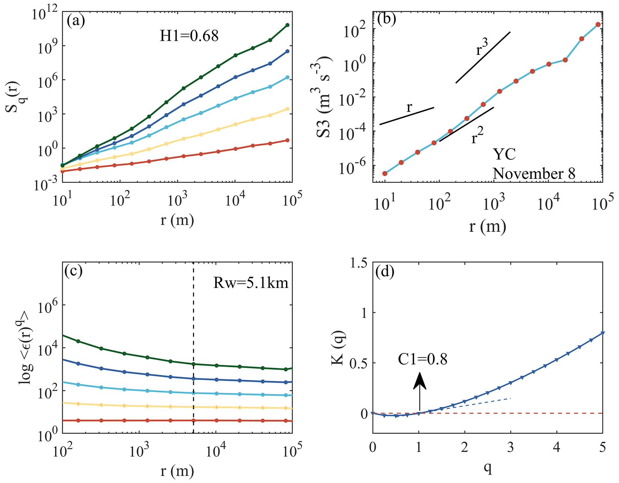
Figure 3 The panels show (a) a multi-order structure function, (b) a third-order structure function (the red dots represent negative values), (c) a multi-order singular measure, and (d) the slope K(q) obtained from the Yichang site in the afternoon of 8 November. In panel (d), the dashed red line is K(q)=0 and the dashed blue line is the fitted slope at K(1).

Figure 4 shows cases of the coexistence of GWs and turbulence as well as unstable GWs. The case of Yichang data from the afternoon of 15 October can be identified as a GW coexisting with turbulence, with a scale of 5.1 km. The GW is quantified as (0.59, 0.10), where the first value is H1 and the second value is C1. The case of Yichang data from the afternoon of 22 November can be identified as an unstable GW, and the GW is quantified as (0.50, 0.12), with a scale of 3.1 km.

By comparing the case results of Figs. 3 and 4, a multi-order structure function (third-order structure function) can be found to have spectral shape differences at certain scales, which mainly come from the intervals with significant inclinations accompanied by a relatively large increase or decrease in the speed increment u_L(r) on these intervals (Fig. A3). As S_q(r)= $\langle \left|{\mathit{\delta }}_{u_L}\right(r){|}^q\rangle$, when the curve of S_q(r) at a certain separation distance r has an obvious inflection point, it means that there is a sudden increase or decrease in some velocity increment in the set of all velocity increments at this scale (He et al., 2022).

For the stable GW (the Yichang site in the afternoon of 8 November), the flat-floating trajectory moves approximately along a quasi-straight line (Fig. A3b), reflecting a relatively single-phase flow region, which indicates that the internal instability of atmospheric wind field fluctuations is relatively weak. For the coexistence of GWs and turbulence (the Yichang site in the afternoon of 15 October) and the unstable gravity wave (the Yichang site in the morning of 3 November), the flat-floating trajectory has been significantly deflected (Fig. A3d, A3f), indicating that the detection area contains different physical flow regions, which means that the internal instability of atmospheric wind field fluctuations is relatively strong. Obviously, this also caused the sawtooth structure in the spectral shape and the inconsistency in the energy cascade direction of the third-order structure function.

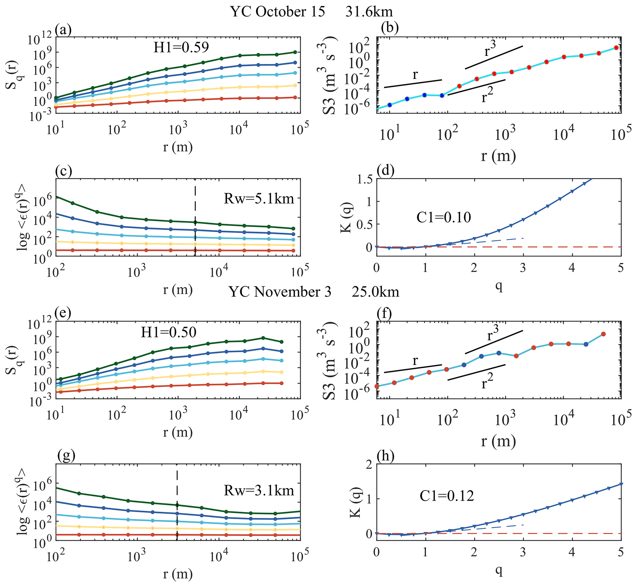
Figure 4 The panels show (a) a multi-order structure function, (b) a third-order structure function, (c) a multi-order singular measure, and (d) the slope K(q) obtained from the Yichang site in the afternoon of 15 October as well as (e) a multi-order structure function, (f) a third-order structure function, (g) a multi-order singular measure, and (h) the slope K(q) obtained from the Yichang site in the morning of 3 November.

Therefore, when the stratospheric disturbance information is relatively abstract, the disturbance intensity can be quantified using (H1, C1) as a reference for mutual comparison. Considering that the calculation of wind speed comes from the coordinates of the positioning system, it is necessary to make sure that there are no wild values interfering with the results. The difference between the positioning coordinates from adjacent times can help identify abnormal positioning data situations – that is, whether there are obvious wild values in the difference in the longitude or latitude. Figure A4 shows cases of abnormal and normal positioning data, and these abnormal cases are screened out. Figure 5a and b show the histogram of Hurst parameters and intermittent parameters for all data from the six sites, respectively. In summer, the H1 (C1) value is mainly concentrated in the range of 0.6–0.8 (0.08–0.16), whereas the H1 (C1) value is mainly concentrated in the range of 0.5–0.7 (0.06–0.14) in autumn. Compared with summer, stratospheric wave disturbances in autumn have a lower H1 and C1 distribution. It is reasonable to have a lower H1 distribution in autumn, as the flat-floating trajectories of the six sites in autumn are more irregular. The obvious change in the trajectory (away from the previous straight direction) indicates that the detected data contain different physical flow regions, suggesting the internal instability and multifractal characterizations of the background wind field fluctuations (Lu and Koch, 2008).

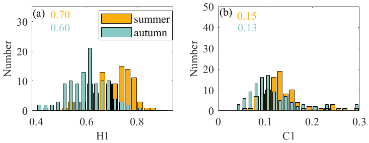
Figure 5 Histograms of (a) the Hurst index and (b) the intermittent parameter from all flat-floating data over the six sites.

4.3 Statistical results of disturbance parameters

The distribution of IGW and turbulence parameters is shown in Fig. 6. The wavelength, intrinsic frequency, and energy of IGWs in summer and autumn show no obvious differences. The momentum flux in summer has a significant positive shift: the net zonal momentum flux is eastward with easterly winds dominant in the stratosphere. The dominant propagation directions of IGWs in summer and autumn are northeast and southwest, respectively, due to the effect of “critical-layer filtering” (Eckermann, 1995). The background wind field filters out GWs propagating in the same direction and passes through GWs propagating in the opposite direction. For disturbances from small-scale turbulence, there is no obvious difference between the Thorpe length and turbulence thickness in summer and autumn. In autumn, the turbulent kinetic energy dissipation rate and turbulent diffusion coefficient have a more ideal Gaussian distribution with a smaller peak value, indicating that the wave source is more specific and the turbulence activity is weaker than that in summer. The deviation of turbulence peaks in different studies may come from the intermittency of turbulence, sensor performance, and regional source characteristics (Ko and Chun, 2022; Zhang et al., 2019; Lv et al., 2021).

In this paper, the vertical wavelength of IGWs is concentrated in the range of 1–3 km, which is close to the scale of stratospheric IGWs in China (1.5–3 km) observed by radiosonde data (Bai et al., 2016). In our results, the kinetic energy and potential energy of IGWs are concentrated at 2–6 and 0–2 J kg⁻¹, respectively. In the tropics, in contrast, the kinetic energy of stratospheric IGWs has already exceeded 10 J kg⁻¹ (Nath et al., 2009), indicating more intense wave activity at lower latitudes. The turbulent kinetic energy dissipation rate log₁₀ε is between −5 and −2 from the RTISS, which is comparable to values obtained based on radiosonde data in the United States, from −4 to −0.5 m² s⁻³ (Ko and Chun, 2022), and in Guam, from −6 to 0 m² s⁻³ (He et al., 2020a).

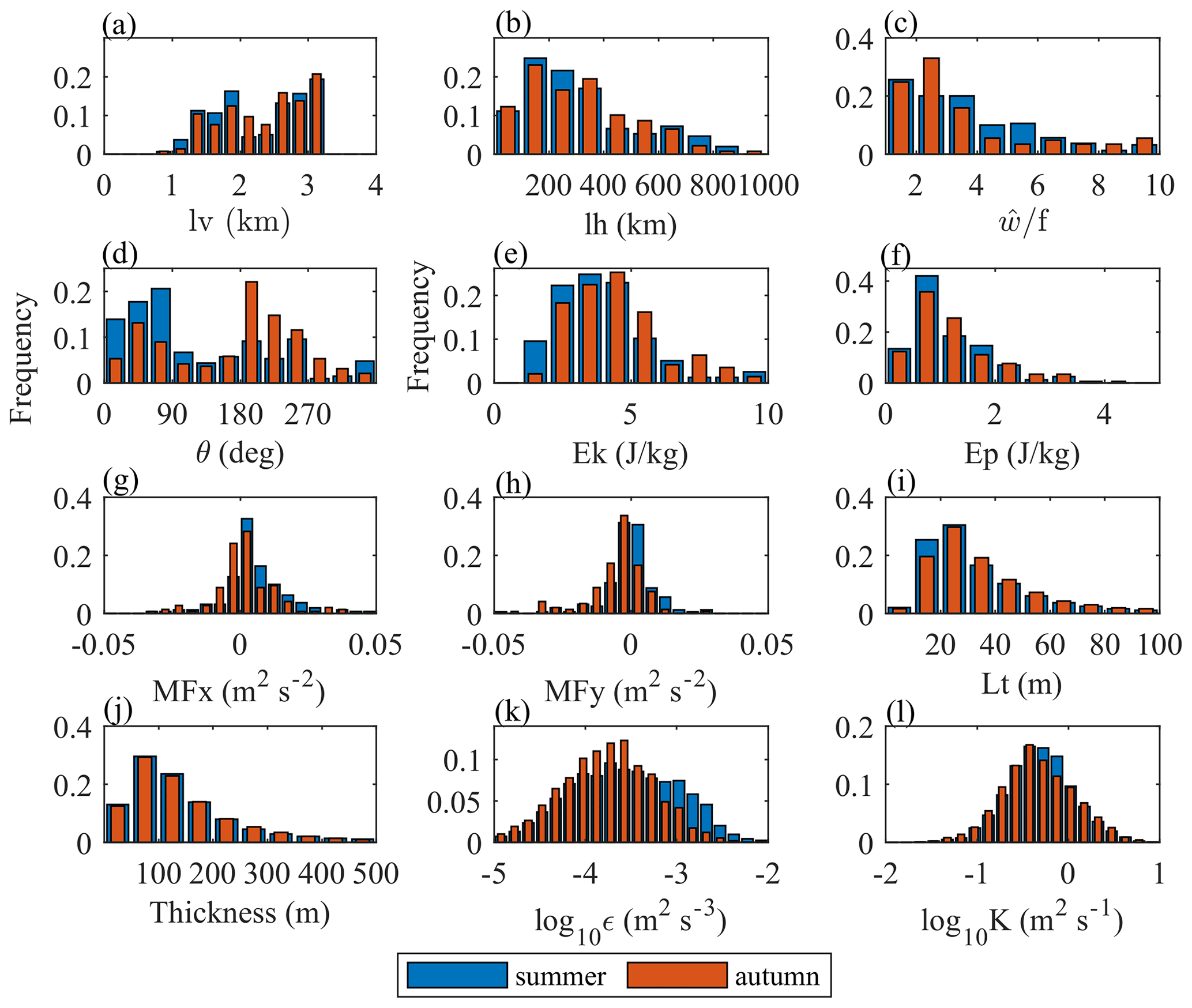
Figure 6 Histograms of the disturbance parameters for IGWs, including the (a) vertical wavelength, (b) horizontal wavelength, (c) intrinsic frequency, (d) horizontal propagation direction, (e) kinetic energy, (f) potential energy, (g) zonal momentum flux, and (h) meridional momentum flux, and of the disturbance parameters for turbulence, including the (i) Thorpe length, (j) turbulent layer thickness, (k) turbulent kinetic energy dissipation rate, and (l) turbulent diffusion coefficient.

The results of H1 and C1 over the six sites are shown in Fig. 7. Compared with the coexistence of GWs and turbulence or unstable GWs, stable GWs tend to have a larger H1 and a smaller C1. The cases in red rectangles are the detection of adjacent times for which the flat-floating height is close; these cases are convenient for the comparison of the third-order structure functions and the wind speed disturbance behind the different (H1, C1) values (the result is shown in Fig. 8). The value of H1 is related to the smoothness of the data series – that is, the denser the wave packets superimposed on the fluctuation trend, the smaller the H1. The value of C1 is related to the singularity degree of the data series – that is, the more disturbances that deviate significantly from the mean state in a local region, the larger the C1 value. The protruding part of the magenta circle in Fig. 8 is the local area of the disturbance sequence (the one with the larger C1 value) that causes the intermittent parameter to be too large. Taking two cases from GZW (the results of Ganzhou in autumn) as examples (Fig. 8), compared with the detection in the afternoon of 17 October, the detection in the afternoon of 20 October has a smaller H1 and a larger C1. The data series in the afternoon of 20 October is rougher with denser wave packets, and there are more obvious strong perturbations that deviate from the mean state in the local area. This is the first time that a relatively comprehensive (multi-site and multi-time) result of stratospheric atmospheric disturbance information in the horizontal direction has been given by balloon observation in China, and it can provide an intuitive reference for the cognition of the stratospheric atmospheric environment.

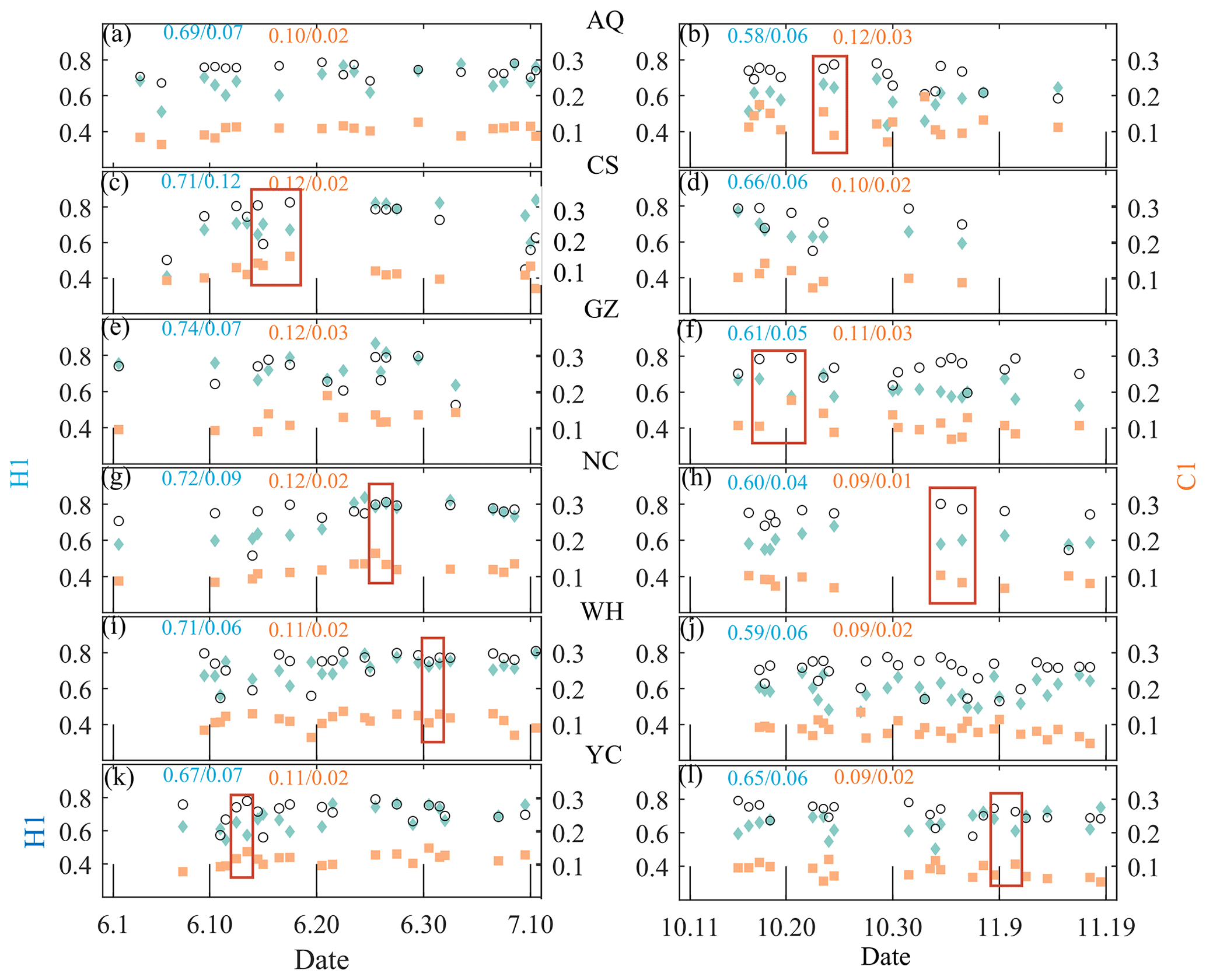
Figure 7 The panels show the atmospheric disturbance parameters (H1, C1) and the corresponding average flat-floating height (scaled to $\mathrm{1}/\mathrm{40}$) obtained over the six sites in summer (a, c, e, g, i, k) and autumn (b, d, f, h, j, l). The mean and standard deviation of H1 and C1 are marked in blue and yellow, respectively.

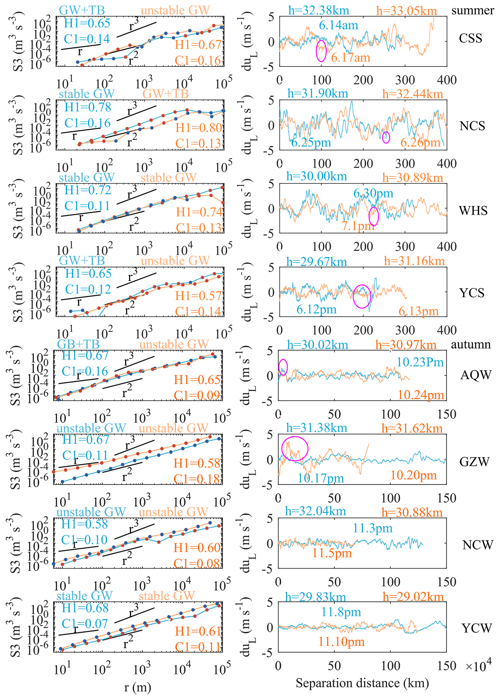
Figure 8 The third-order structure function (left) and the longitudinal velocity component perturbation (right) for the selected cases in the corresponding red rectangles in Fig. 7. In order to better compare the roughness and singularity of the velocity component, the longitudinal velocity component perturbation is used here after removing the background field using a fourth-order polynomial fit. The protruding part of the magenta circle is the local area of the disturbance sequence (the one with the larger C1 value) that causes the intermittent parameter to be too large.

4.4 Potential links between multiscale fluctuations

Although there are different methods for quantifying wave disturbances, linking detection results from different profiles (e.g., in the vertical and horizontal directions) is still a challenge and an observation gap. Taking the detection results from the RTISS as an opportunity, the possible connection between wave disturbances obtained by different quantitative methods is discussed, and the result is shown in Fig. 9. It should be noted here that the wave disturbances extracted from the flat-floating data are small-scale, high-frequency GWs with a spatial scale of several kilometers, whereas the wave disturbances extracted from the rising data are IGWs with a spatial range of several hundred kilometers. There is no clear linear correlation between H1 and C1 (Fig. 9a). C1 can reflect the intensity of turbulence mixing and is highly intermittent and random, which is not related to height (Fig. 9b). In contrast, there is a significant positive linear correlation between H1 and height (Fig. 9c). As height increases, the entire data series tends to be smoother.

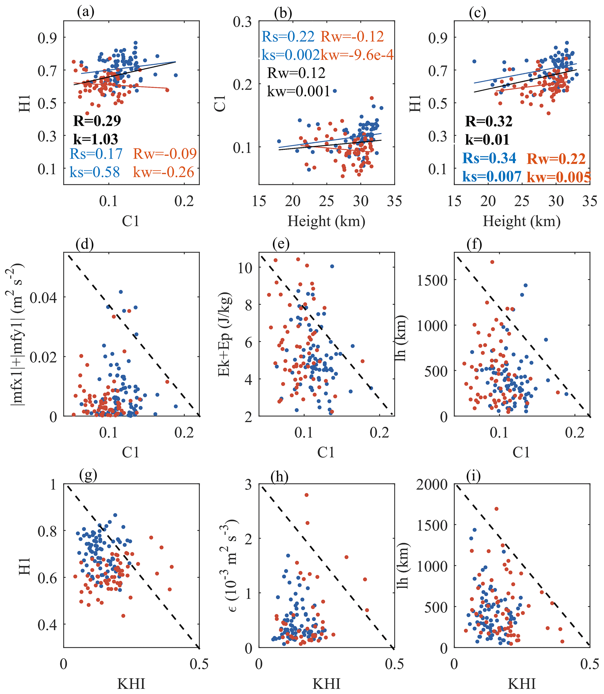
Figure 9 Scatterplots of (a) H1 versus C1, (b) C1 versus height, (c) H1 versus height, (d) momentum flux versus C1, (e) total energy versus C1, (f) horizontal wavelength versus C1, (g) H1 versus KHI (ratio of $\mathrm{0}<Ri<$ 0.25), (h) ε versus KHI, and (i) horizontal wavelength versus KHI. Blue and red dots represent summer and autumn, respectively. The blue, red, and black lines in panels (a), (b), and (c) represent the linear fitting results of summer, autumn, and all data, respectively.

Due to the limitations of the sample size and the different detection objects, the linear correlation between these variables from Fig. 9d, e, and f may not be statistically significant, so we pay more attention to the change trend between them. With an increase in C1, the momentum flux, total energy, and horizontal wavelength of IGWs are more concentrated in a lower range (Fig. 9d, e, f). Next, we consider that the wave disturbance in the stratosphere is likely to be related to the Kelvin–Helmholtz instability (KHI) (He et al., 2020b; Lu and Koch, 2008). The ratio of $\mathrm{0}<Ri<$ 0.25 between 15 and 25 km represents the instability. As the KHI increases, the horizontal wavelength of IGWs decreases (Fig. 9i), whereas the data sequence of SGWs tend to be rougher (Fig. 9g). Although the occurrence of large C1 values (> 0.15) is relatively rare (the detected disturbances with strong intermittence are still low-probability events in the entire sample), it is still possible to see that the enhanced C1 is accompanied by a weakened momentum flux, energy, and horizontal wavelength of IGWs.

From the above results, it can be seen that the increased instability of SGWs in the stratosphere will be accompanied by the weakening of IGWs below. The KHI that appears in an unstable shear due in part to IGWs (Abdilghanie and Diamessis, 2013) is likely to be the excitation source of small-scale, high-frequency GWs propagating to higher altitudes. This phenomenon has also been confirmed by numerical simulations in the mesosphere and at higher altitudes (Dong et al., 2023).

4.5 Relation between the parameter space and ozone transport

The transport of ozone and its changing trends is one of the important issues in stratospheric research and is closely related to the atmospheric radiation balance and global warming (Tian et al., 2023; Fei Xie et al., 2016; Jiankai Zhang et al., 2022; He et al., 2023). The ozone and potential vorticity (PV) have good consistency and can be regarded as good indicators for studying the stratospheric material transport process (Allaart et al., 1993; Newell et al., 1997). Considering that the GW process plays an important role in the transport of ozone between the upper and lower layers (Gabriel, 2022), we aim to explore whether there is a direct connection between the quantitative indicator of wave disturbance and ozone.

Based on the ERA5 reanalysis data, the ozone mass mixing ratio (OMR) and PV at different pressure layers that matched the detection are selected. Specifically, the ERA5 data at 00:00 and 12:00 UTC within the longitude and latitude range of the selected flat-floating stage are screened, and the regional average is used as the reanalysis data result corresponding to the flat-floating detection at that time. The matching results of different air pressure layers (150, 125, 100, 70, 50, 30, 20, 10, 5, and 3 hPa) are calculated.

Figure 10 shows the possible connection between C1 and these two indicators (OMR and PV). The pressure layers selected here correspond to the height above (10 hPa) and below (100 hPa) the flat-floating interval (20–30 km) in order to distinguish them from the height range where small-scale GWs are detected. In the lower stratosphere (100 hPa), there is a significant positive correlation between ozone and PV, whereas in the middle stratosphere (10 hPa), there is a significant negative correlation between the two. For SGWs detected during flat-floating stage, the larger the C1, the weaker the PV in the stratosphere, accompanied by the reduction in IGWs (Kalashnik and Chkhetiani, 2017). This is consistent with the result that a higher C1 corresponds to a lower IGW energy below (seen in Fig. 9). The higher the intermittency of SGWs, the less (more) ozone below (above), thereby forming an enhanced ozone transport from lower to higher altitudes. In the process of area averaging, there are usually only two or three ERA5 data points within the latitude (longitude) range of the flat-floating trajectory. However, as there are still some cases without matched ERA5 data, we extend the latitude (longitude) range to a width extending 0.25° north (east) and south (west) of the center point of the trajectory. In this way, ERA5 data and the trajectory can be matched as much as possible under the premise that there are data in the matching area.

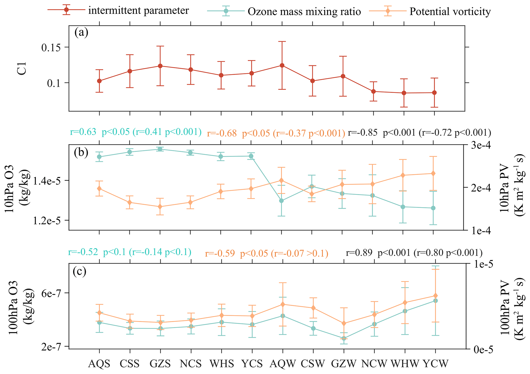
Figure 10 The error bar diagram of (a) intermittent parameters for C1 and the ozone mass mixing ratio (OMR) and potential vorticity (PV) at the (b) 10 hPa and (c) 100 hPa pressure layers in summer (S) and autumn (W), showing a total of 12 clusters over the 6 sites. The blue, yellow, and black annotations marked at the top of the figure panels indicate the Pearson correlation coefficient and significance level for OMR versus C1, PV versus C1, and OMR versus PV, respectively. Values outside of parentheses represent the correlation of the average values of the 12 clusters (12 values), whereas values inside parentheses represent the correlation of all cases of the 12 clusters.

The mechanism diagram of ozone transport and energy transfer is shown in Fig. 11. The significant positive (negative) correlation between C1 and the ozone concentration in the lower (middle) stratosphere further supports the argument that SGWs may affect the vertical transport of ozone (Fig. 11, right). The stratospheric SGWs detected here are closely related to the KHI, and previous studies have also confirmed this (He et al., 2020b; Lu and Koch, 2008). The transport capacity of IGWs with respect to ozone is weakened due to critical-layer filtering during its upward propagation. In contrast, the high-frequency SGWs can propagate to higher altitudes (Dong et al., 2023). Ozone transport is closely related to the SGWs between 100 and 10 hPa, corresponding to a weakening of IGWs in the lower stratosphere (100 hPa) and an enhancement of SGWs excited by the KHI. SGWs with higher phase velocities would propagate upward without encountering a critical level and, thus, complete ozone transport to the middle stratosphere (10 hPa) (Heale and Snively, 2015; Li et al., 2020; He et al., 2022b). Enhanced intermittency is accompanied by the weakening of IGW energy below, which also reveals possible energy transfer from large-scale to small-scale waves.

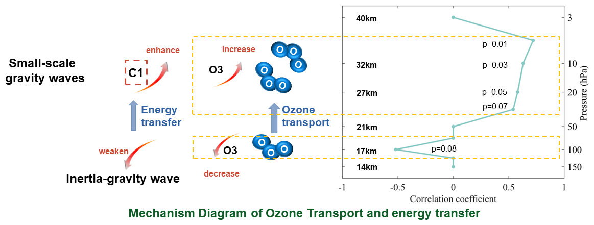
Figure 11 The mechanism diagram of ozone transport and energy transfer. The right-hand side of the figure shows the vertical distribution of the correlation coefficient between the OMR and C1 in summer and autumn (a total of 12 clusters) over the 6 sites at different pressure layers. When the correlation for OMR versus C1 of the average values of the 12 clusters (12 values) and of all cases are both statistically significant (p<0.1), it is considered that the small-scale GW disturbance is closely related to the change in the ozone concentration at the corresponding pressure layers; otherwise, the correlation coefficient is set to zero. For the pressure layers with a significant correlation coefficient, the significance level (p value) corresponding to the 12 clusters is marked on the left-hand side of the figure.

4.6 Calculation for a single-phase flow regime

Two scales, shown as the inconsistency in the energy cascade direction, are related to different physical flow regimes (Lu and Koch, 2008). In balloon observations, these different physical flow regimes will be represented by curved (nonlinear) trajectories. Therefore, in order to retain this recognition of different physical flow regions, zonal or meridional projection is selected (which can decompose the curved trajectory into zonal or meridional), as shown above. In this section, we also use the method of linear fitting to show the calculation results of a single-phase flow regime.

The YC case on 15 October is taken as an example to illustrate this method (shown in Fig. 12). In order to ensure quasi-linear fitting, the region that can be approximated as a straight line for linear fitting is selected from the original flat-floating trajectory. The selected period is represented by the orange rectangle in Fig. 12a. The data that can be processed by line fitting are then shown in Fig. 12b. By decomposing the zonal and meridional wind components into a new coordinate system (the x axis is parallel to the fitted line), the longitudinal (along the separation distance direction) and transverse (normal to the separation distance direction) velocity components can be obtained (Fig. 12c, d).

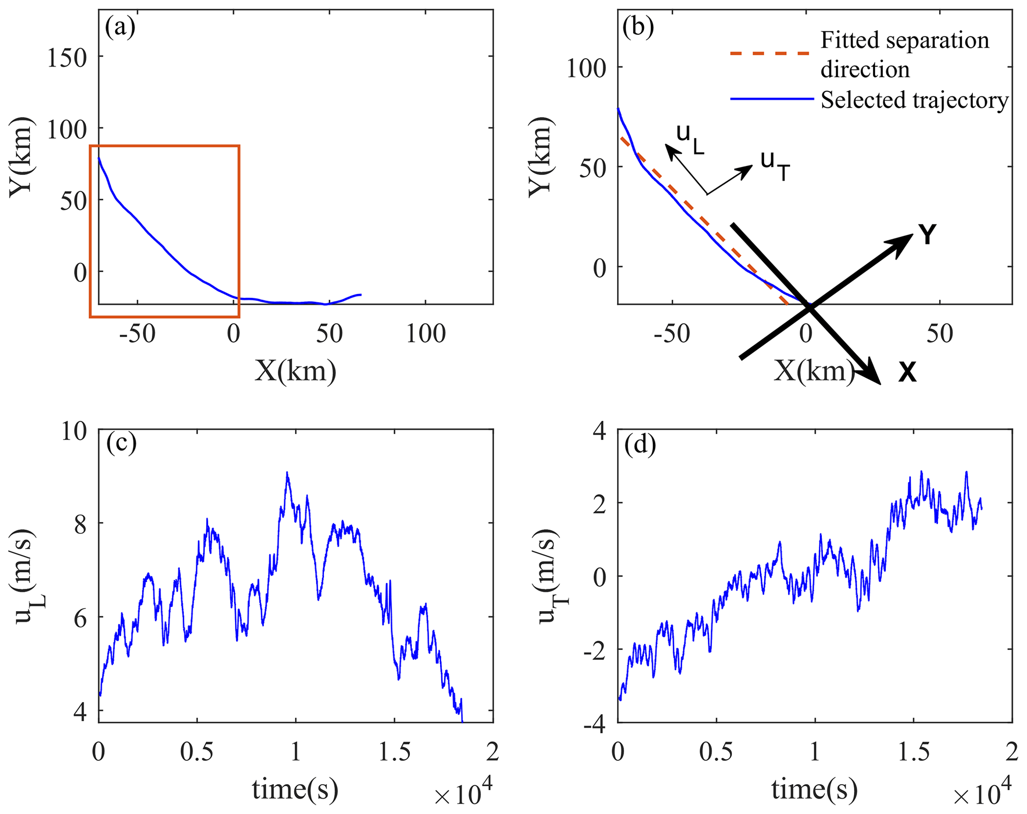
Figure 12 The trajectory in the X–O–Y plane (a) before and (b) after quasi-linear fitting as well as (c) the longitudinal (along the fitted line) velocity u_L and (d) the transverse (normal to the fitted line) velocity u_T after quasi-linear fitting from the Yichang site in the afternoon of 15 October.

Furthermore, the third-order structure function and slope K(q) curve in the single-phase flow region are obtained, as shown in Fig. 13. Compared with the zonal projection of the multi-phase flow regime (Fig. 4b, d), the calculated results of the single-phase flow regime may be different for both H1 and C1, especially for H1. The reason for this is that, in the process of linear fitting, partial trajectories that deviate significantly from the straight line are omitted. According to Eq. (1), the inconsistency between the convergence and divergence of velocity on adjacent scales leads to internal instability. The balloon itself moves with the wind; thus, when there is a sudden change in the velocity field, the flat-floating trajectory will naturally change. If the trajectory direction is relatively defined (single-phase flow region), the linear fitting method can actually get more accurate results. However, the problem is that, as many curved trajectories are rounded out after screening, the results obtained are not suitable for internal comparison. Furthermore, irregularly curved trajectories may also contain important disturbance information. Compared with the best linear fitting of the single-phase flow region, the zonal or meridional projection in the multi-phase flow zone can be said to be a compromise method. Not only can more samples be retained but disturbance information behind the curved/irregular trajectories can also be retained.

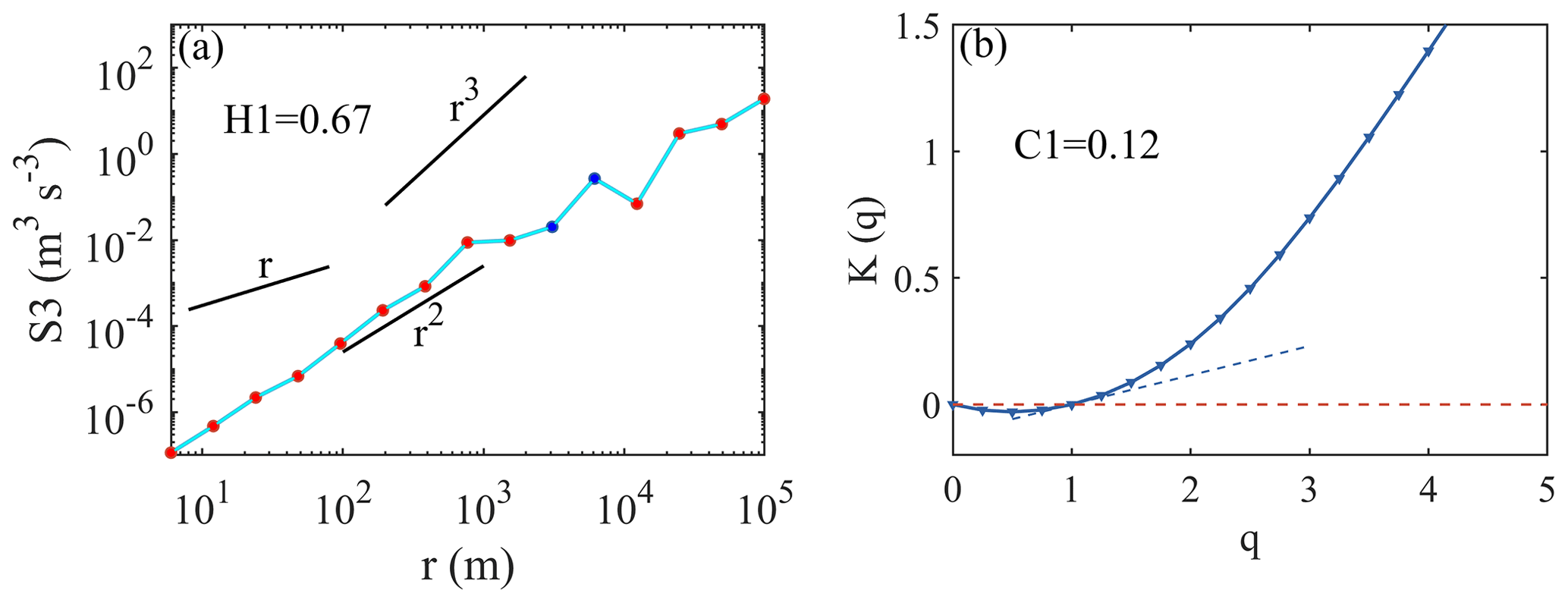
Figure 13 The (a) third-order structure function and (b) slope K(q) obtained from the Yichang site in the afternoon of 15 October.

5 Summary and conclusion

Based on the round-trip intelligent sounding system (RTISS) released in China, we conducted a systematic analysis on atmospheric disturbance information from the stratosphere. Using the structure function and singular measurement relationships, the parameter space (H1, C1) is calculated to describe the nonstationarity and intermittency of atmospheric dynamic processes. The physical process corresponding to stratospheric SGWs is mapped to this parameter space, realizing the comparison of disturbance characteristics between different cases (difference in flat-floating height as well as time and space). There is a significant linear relationship between H1 and height. As height increases, the nonstationarity (roughness) decreases. In contrast, the distribution of C1 is more random and independent of height, and the intensity of turbulence mixing and SGWs at different altitudes can be compared.

Continuous detection from rising and flat-floating stages realizes the seamless capture of stratospheric SGWs and IGWs below them. By analyzing the correlation between the parameters calculated by multiscale disturbances, the connection between IGWs and SGWs is qualitatively revealed. The results show that the enhancement of SGWs is accompanied by a weakening of IGW activity below, and the generation of these SGWs is related to the KHI. In addition, we explored the role of GWs in stratospheric ozone transport based on the potential relationship between the intermittent parameter C1, potential vorticity, and ozone, and we found that the enhancement of SGWs is conducive to the transport of ozone from the lower stratosphere to higher altitudes, although the length of this path is limited due to the wave dissipation. This is the first time that a high-frequency, long-duration in situ detection method has been used to discuss the role of stratospheric multiscale disturbances in energy transfer and material transport in China. The introduction of flat-floating information provides a new idea for the study of stratospheric dynamic processes, while three-stage detection supplements the research of stratosphere–troposphere interactions (Scaife et al., 2012; Niu et al., 2023).

Encouragingly, the quantitative description of SGWs in the stratosphere using (H1, C1) values has shown a possible connection with larger-scale IGWs and smaller-scale turbulence, and a potential relationship between SGWs and stratospheric ozone transport can be found. Of course, given the limited number of samples and the different perturbation extraction methods in the vertical and horizontal directions, the potential connection between these multiscale fluctuations may not be significant. However, the linear relationship between disturbance from IGW and SGW can be significant if only kinetic energy is considered (the calculation of the disturbance parameter in SGWs is derived only from the wind speed), as shown in Fig. A5. This also indicates that the enhancement of SGWs is indeed accompanied by the weakening of IGWs. Moreover, regardless of whether the flat-floating trajectory has been linearly fitted or not, this significant linear relationship exists.

The SGWs captured by the flat-floating balloon discussed are mainly concentrated in the stratospheric altitude range of 20–30 km. However, it should be noted that this does not mean that the SGW activity outside of this altitude range can be ignored (including the upward propagation of SGW inside the altitude range and the undetected SGWs outside of the altitude range), which is a possible reason for the significant positive correlation between C1 and ozone at higher altitudes (the positive correlation on the 5 hPa pressure layer in Fig. 11). Considering that an initial ascent of an air parcel can lead to an increase (decrease) in ozone above (below) compared with the surrounding atmosphere, the general positive correlation between C1 and ozone within the height range where SGWs are detected shows that the propagation direction of SGWs is mainly upward.

Use of the RTISS provides an opportunity for related research: that is, it is possible to achieve quasi-seamless detection of the atmospheric structure from both the vertical and horizontal directions inside the stratosphere at the same time. The relatively high resolution is also conducive to better capturing the fine structure of atmospheric disturbances. Taking the IGWs and SGWs studied in this paper as an example, the effective capture of different disturbances in continuous time based on the RTISS on different cross-sections is impossible to achieve with other single-measurement methods. Due to the sample size limitation and the differences in calculation methods, there may be some not completely significant relationships in the discussion of different wave types and their relationship with ozone. However, the exploration of stratospheric atmospheric disturbances and material transport using this new detection method is still worthy of continuous follow-up and improvement. As valid samples gradually accumulate, these relationships may become more significant and robust.

Our results reveal the important role of stratospheric SGWs in material transport and energy transfer as well as demonstrating the potential ability of the physical parameter space (H1, C1) in stratospheric dynamics research. Follow-up research is worth continuing, using the detection results of the RTISS in more regions with longer periods, to improve our understanding of the statistical characteristics and regional differences in stratospheric disturbance information. Moreover, potential connections that may exist between this parameter space and other atmospheric components (such as water vapor, carbon dioxide, and methane) transported in the stratosphere also deserves further attention.

Appendix A

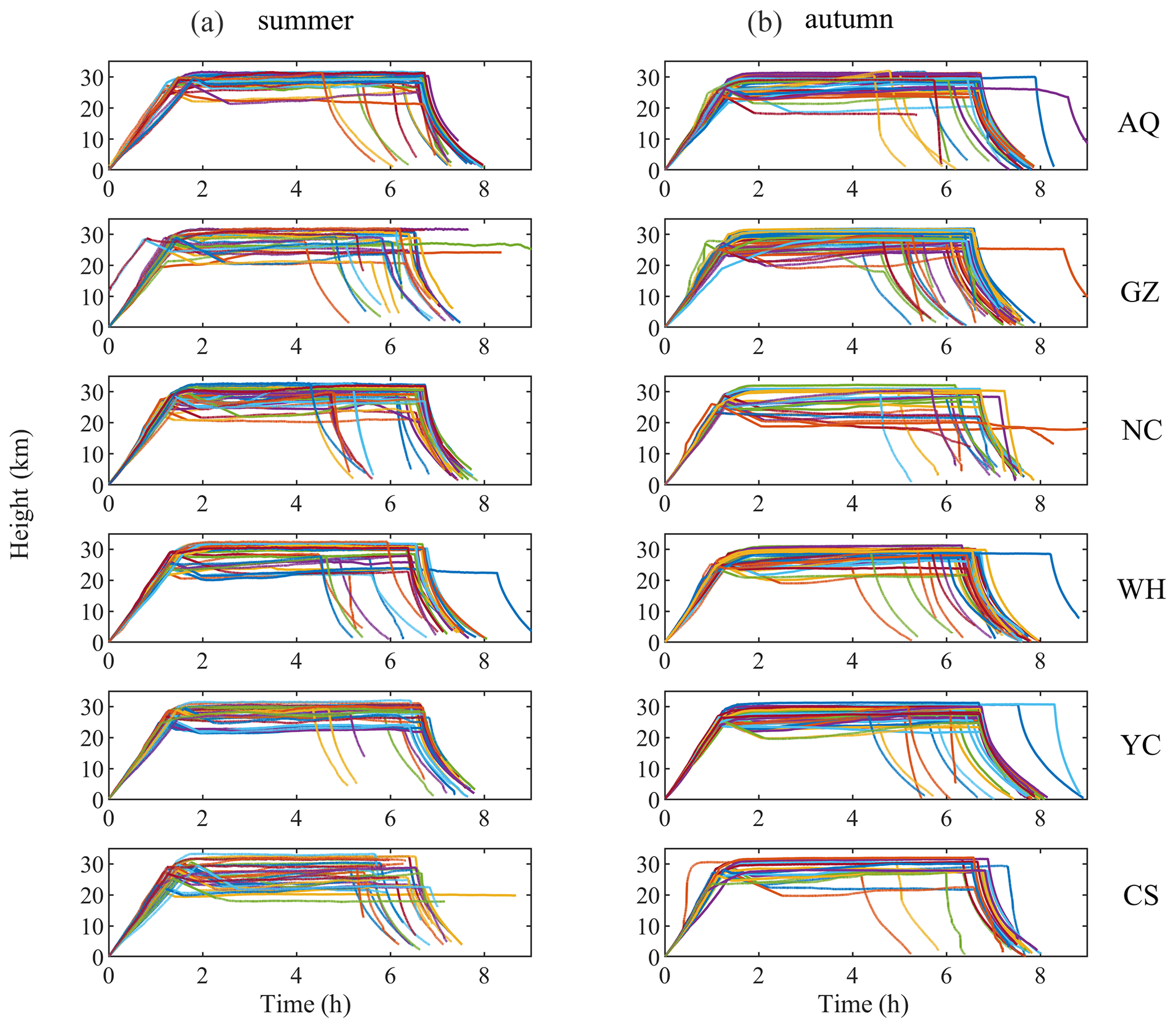
Figure A1 Time–height curves in summer (a) and autumn (b) during the entire detection process for RTISS detections at six sites.

Figure A2 Velocity increments calculated from the beginning to the end of the data series from the Yichang site on 8 November for separation distances of (a) 44 m, (b) 352 m, (c) 5600 m, and (d) 45 056 m.

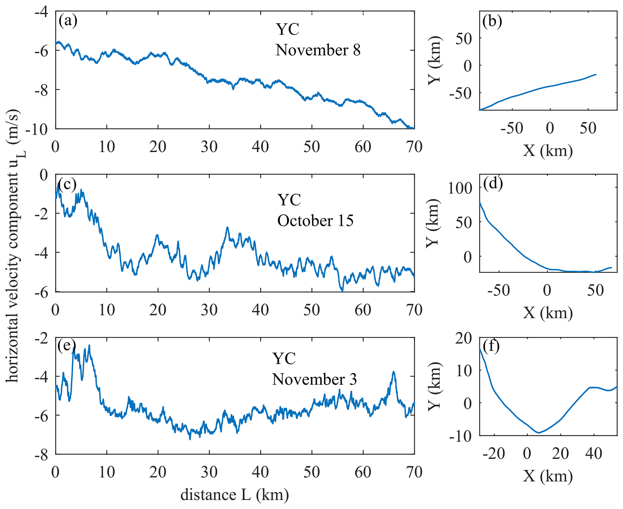
Figure A3 The variation in the horizontal velocity component u_L along the zonal separation distance (a, c, e) and flat-floating trajectory (b, d, f) from three cases.

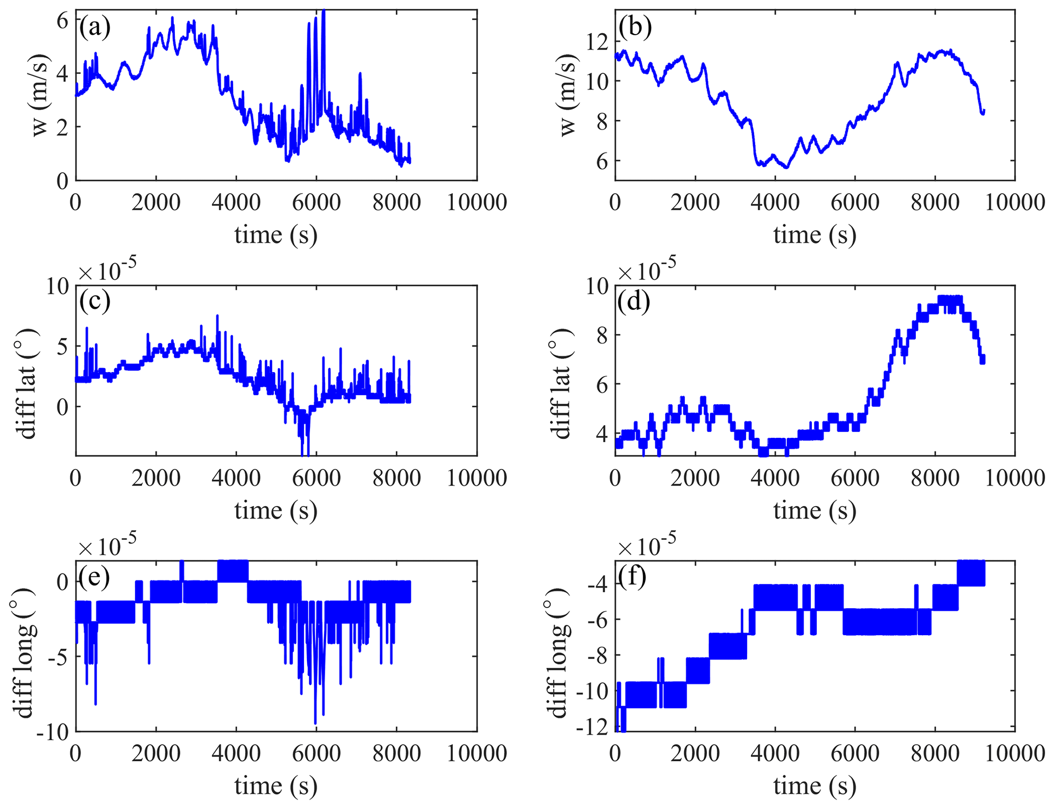
Figure A4 The (a) wind velocity, (c) latitude difference, and (e) longitude difference for the case where the positioning data are abnormal; the (b) wind velocity, (d) latitude difference, and (f) longitude difference for the case where the positioning data are normal.

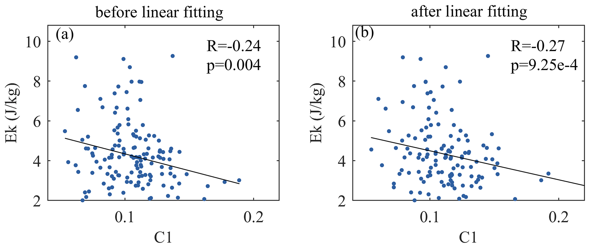
Figure A5 Scatterplots of kinetic energy (Ek) versus C1 (a) before linear fitting and (b) after linear fitting.