Multidecadal ozone trends in China and implications for human health and crop yields: a hybrid approach combining a chemical transport model and machine learning

Surface ozone (O₃) is well known for posing significant threats to both human health and crop production worldwide. However, a multidecadal assessment of the impacts of O₃ on public health and crop yields in China is lacking due to insufficient long-term continuous O₃ observations. In this study, we used a machine learning (ML) algorithm to correct the biases of O₃ concentrations simulated by a chemical transport model from 1981–2019 by integrating multi-source datasets. The ML-enabled bias correction offers improved performance in reproducing observed O₃ concentrations and thus further improves our estimates of the impacts of O₃ on human health and crop yields. The warm-season trends of increasing O₃ in Beijing–Tianjin–Hebei and its surroundings (BTHs) as well as in the Yangtze River Delta (YRD), Sichuan Basin (SCB), and Pearl River Delta (PRD) regions are 0.32, 0.63, 0.84, and 0.81 µg m⁻³ yr⁻¹ from 1981 to 2019, respectively. In more recent years, O₃ concentrations experienced more fluctuations in the four major regions. Our results show that only BTHs have a perceptible increasing trend of 0.81 µg m⁻³ yr⁻¹ during 2013–2019. Using accumulated O₃ over a threshold of 40 ppb (AOT40-China) exposure–yield response relationships, the estimated relative yield losses (RYLs) for wheat, rice, soybean, and maize are 17.6 %, 13.8 %, 11.3 %, and 7.3 % in 1981, increasing to 24.2 %, 17.5 %, 16.3 %, and 9.8 % in 2019, with an increasing rate of +0.03 % yr⁻¹, +0.04 % yr⁻¹, +0.27 % yr⁻¹, and +0.13 % yr⁻¹, respectively. The estimated annual all-cause premature deaths induced by O₃ increased from ∼55 900 in 1981 to ∼162 000 in 2019 with an increasing trend of ∼2980 deaths per year. The annual premature deaths related to respiratory and cardiovascular disease are ∼34 200 and ∼40 300 in 1998 and ∼26 500 and ∼79 000 in 2019, having a rate of change of −546 and +1770 deaths per year during 1998–2019, respectively. Our study, for the first time, used ML to provide a robust dataset of O₃ concentrations over the past 4 decades in China, enabling a long-term evaluation of O₃-induced crop losses and health impacts. These findings are expected to fill the gap of the long-term O₃ trend and impact assessment in China.

1 Introduction

Surface ozone (O₃), an important secondary air pollutant, is mainly generated through photochemical reaction of volatile organic compounds (VOCs), carbon monoxide (CO), and nitrogen oxides (NO_x) in the presence of sunlight. As a strong oxidant, O₃ at the ground level is detrimental to human health and vegetation. More recently, due to rapid urbanization and industrialization, summertime O₃ pollution has become an emerging concern in China. Li et al. (2020) reported that the mean summer 2013–2019 trend in maximum daily 8 h average surface O₃ (MDA8 O₃) was +1.9 ppb yr⁻¹ in China, with high values widely observed in the North China Plain (NCP), Yangtze River Delta (YRD), and Pearl River Delta (PRD) regions. On the regional scale, the exposure of humans and vegetation to O₃ is greater in China than in other developed regions of the world (Lu et al., 2018). Several studies have suggested that climate and land cover changes play an important role in O₃ pollution in addition to anthropogenic emissions (Fu and Tai, 2015; Wang et al., 2020). It has been suggested that global warming and the changing land use may further increase surface O₃ by the late 21st century (Kawase et al., 2011; Wang et al., 2020), which can pose greater threats to human health and food security.

Meteorological factors can modulate the temporal and spatial patterns of O₃ by affecting the physical and chemical processes within the atmosphere (Liu et al., 2019; Mao et al., 2020; Yin and Ma, 2020). High temperature, low relative humidity, and low planetary boundary height are conducive to photochemical production and O₃ accumulation. Jacob and Winner (2009) summarized that the enhanced O₃ levels at higher temperatures are primarily driven by increased biogenic VOC emissions from vegetation and reduced lifetimes of peroxyacetyl nitrate (PAN) due to accelerated decomposition of PAN into NO_x. Moreover, the changes in wind speed and direction can affect O₃ concentrations through transport. Land cover and land use change affects O₃ air quality by perturbing surface fluxes, hydrometeorology, and concentrations of atmospheric chemical components (Tai et al., 2013; Fu and Tai, 2015; Liu et al., 2020; Ma et al., 2021). For instance, the terrestrial biosphere is a major source of isoprene, which plays a significant role in modulating O₃ concentrations. In the Intergovernmental Panel on Climate Change (IPCC) A1B scenario, Tai et al. (2013) found that widespread crop expansion could reduce isoprene emission by ∼10 % globally compared with the present land use. Such a reduction could decrease O₃ by up to 4 ppb in the eastern US and increase O₃ by up to 6 ppb in southern and southeastern Asia, whereby the difference in the sign of responses is primarily determined by the different O₃ production regimes.

The increasing health burden due to air pollution has become an important contributor to the global burden of disease. Some recent studies have demonstrated that short-term O₃ exposure negatively impacts human health, especially with respect to respiratory and cardiovascular mortality (Shang et al., 2013; P. Yin et al., 2017; Feng et al., 2019; Zhang et al., 2022a). In 2015–2018, the estimated annual total premature mortality related to O₃ pollution in 334 Chinese cities was 0.27 million for 2015, 0.28 million for 2016, 0.39 million for 2017, and 0.32 million for 2018 (Zhang et al., 2021). Maji and Namdeo (2021) reported that short-term all-cause, cardiovascular, and respiratory premature mortalities attributed to the ambient fourth-highest MDA8 O₃ exposure were 156 000, 73 500, and 28 600 in 2019, showing increases of 19.6 %, 19.8 %, and 21.2 %, respectively, compared to 2015. Zhang et al. (2022b) reported that each 10 µg m⁻³ increase in the MDA8 O₃ can lead to a rise of 0.41 % (95 % CI: 0.35 %–0.48 %) in all-cause mortality, 0.60 % (95 % CI: 0.51 %–0.68 %) in cardiovascular mortality, and 0.45 % (95 % CI: 0.28 %–0.62 %) in respiratory mortality.

The damage to plants induced by O₃ is mainly caused by the stomatal uptake of O₃ into the leaf interior instead of direct plant surface deposition (e.g., Clifton et al., 2020). In previous studies, a variety of concentration-based metrics have been widely used to assess the O₃ risks to crop yield and ecosystem functions. Initially, a 7 h (09:00–15:59 LT) mean metric (M7) was proposed, which was later extended to 12 h (08:00–19:59 LT; referred to as M12) to include late-day O₃ concentrations. Cumulative metrics have also been developed to evaluate the impacts of O₃ on crops. The accumulated O₃ over a threshold of 40 ppb (AOT40) is a widely used metric to evaluate the phytotoxic effects of O₃. Compared to AOT40 using a linear function, another metric, W126, considers the nonlinear response of yield loss to O₃ exposure whereby higher O₃ concentrations will progressively induce more severe yield losses. However, many studies have suggested that the stomatal uptake of O₃ is more related to vegetation damage than to O₃ exposure per se (Feng et al., 2012, 2018; Pleijel et al., 2022). Therefore, in the past 2 decades, the flux-based approach has been developed and has increasingly been used to assess the relationships between the stomatal O₃ uptake and crop yields. Tai et al. (2021) compared the results of the estimated global crop yield losses using three concentration-based and two flux-based O₃-exposure metrics and showed that the concentration-based metrics differ greatly among themselves, while the two flux-based metrics, which lie close to the middle of the range covered by all metrics, are generally close to each other.

At present, a comprehensive long-term assessment of the impacts of O₃ is hindered by a lack of continuous O₃ observations in China (Lu et al., 2018; Gong et al., 2021). From both health and food perspectives, reliable long-term estimates of O₃ are critically needed to better understand O₃ damage over the past few decades since the beginning of rapid industrial transformation in the 1980s. In previous studies, various alternative approaches have been used to address the problem of insufficient observations. The multiple linear regression (MLR) model is often used for extrapolation to construct spatiotemporal distributions of air pollutants (Moustris et al., 2012; Abdullah et al., 2017). However, these linear statistical methods are generally limited by their incapability to capture the nonlinear relationships between air pollutants and precursors as well as meteorological fields. Chemical transport models (CTMs), based on mathematical representation of atmospheric physical and chemical processes, are also a common tool to simulate air pollutant concentrations spatiotemporally (Fusco and Logan, 2003; Liu and Wang, 2020a; H. Wang et al., 2022). Taking advantage of the CTM, Fu and Tai (2015) investigated the impacts of historical climate and land cover changes on tropospheric O₃ in eastern Asia between 1980 and 2010. However, the utility of CTMs is often limited by their high computational cost when conducting long-term simulations at high spatiotemporal resolutions. Large biases also exist due to uncertainties in historical emission inventories, parameterization of physical and chemical processes, and initial and/or boundary conditions, and these errors tend to increase at finer spatiotemporal scales.

In recent years, machine learning (ML) methods have gained increasing popularity in air pollution studies (Liu et al., 2020; Ma et al., 2021). In the early stage of applying ML to atmospheric chemistry, ML methods were usually used as an independent method from CTMs (Hu et al., 2017; Zhan et al., 2017), for instance, to predict O₃ concentrations by mapping the nonlinear relationships between observed O₃ concentrations and their possible shaping factors. These applications are usually purely data-driven, whereby the ML algorithms do not involve any representation of the physical mechanisms behind the relevant processes. With powerful algorithms and user-friendly hyperparameter tuning processes, some well-trained ML models, driven by data from multiple sources including reanalysis and satellite data, have shown even higher predictive capacity than process-based models. The advantages of ML methods over CTMs include more flexible choices for input data and spatiotemporal resolution as well as substantially lower computational costs (Bi et al., 2022). However, purely data-driven ML methods are known for suffering a lack of transparency and interpretability, which renders it more difficult to offer adequate scientific interpretation for the physical mechanisms behind the relevant processes. Thus, a hybrid approach combining ML algorithms and CTM-simulated results has increasingly been used in recent years to predict air pollutants and understand their trends. Integrating data from various sources, ML methods have been used as a tool to correct the biases in the lower-resolution simulated results from CTMs (Di et al., 2017; Ivatt and Evans, 2020; Ma et al., 2021). Based on process-based CTMs integrating decades of accumulated knowledge in Earth system science while taking advantage of ML to address still-existing model errors, the hybrid approach has great potential to tackle air quality problems (Irrgang et al., 2021).

In this work, we incorporated the O₃ concentrations directly simulated by the Goddard Earth Observing System coupled with Chemistry (GEOS-Chem) model at a lower resolution into a bias-corrected, finer-resolution dataset by integrating them with O₃ observations from 2016 to 2018 (for validation purposes), high-resolution meteorological fields, land use data, and other geographical information from multiple sources using a tree-based ML algorithm called LightGBM. The final high-resolution hourly O₃ dataset with a resolution of $\mathrm{0.25}{}^{\circ }\times \mathrm{0.25}{}^{\circ }$ from 1981 to 2019 was further used to assess the impacts of O₃ on human health and crop yields over the past 4 decades. The simultaneous analysis of the combined impacts of O₃ on agriculture and human health can offer more comprehensive policy implications for the mitigation of O₃-related impacts across China.

2 Data and methods

2.1 Air quality, meteorological, land, and crop data

Hourly surface O₃ observations (µg m⁻³) from 2016 to 2018 were obtained from the China National Environmental Monitoring Center Network (https://air.cnemc.cn:18007/, last access: 24 December 2023) established by the Ministry of Ecology and Environment of China. The MDA8 O₃ of each site was calculated with at least 14 valid hourly values from 08:00 to 00:00 LT. A total of 1016 sites were selected after deleting the missing and abnormal data (Fig. 1).

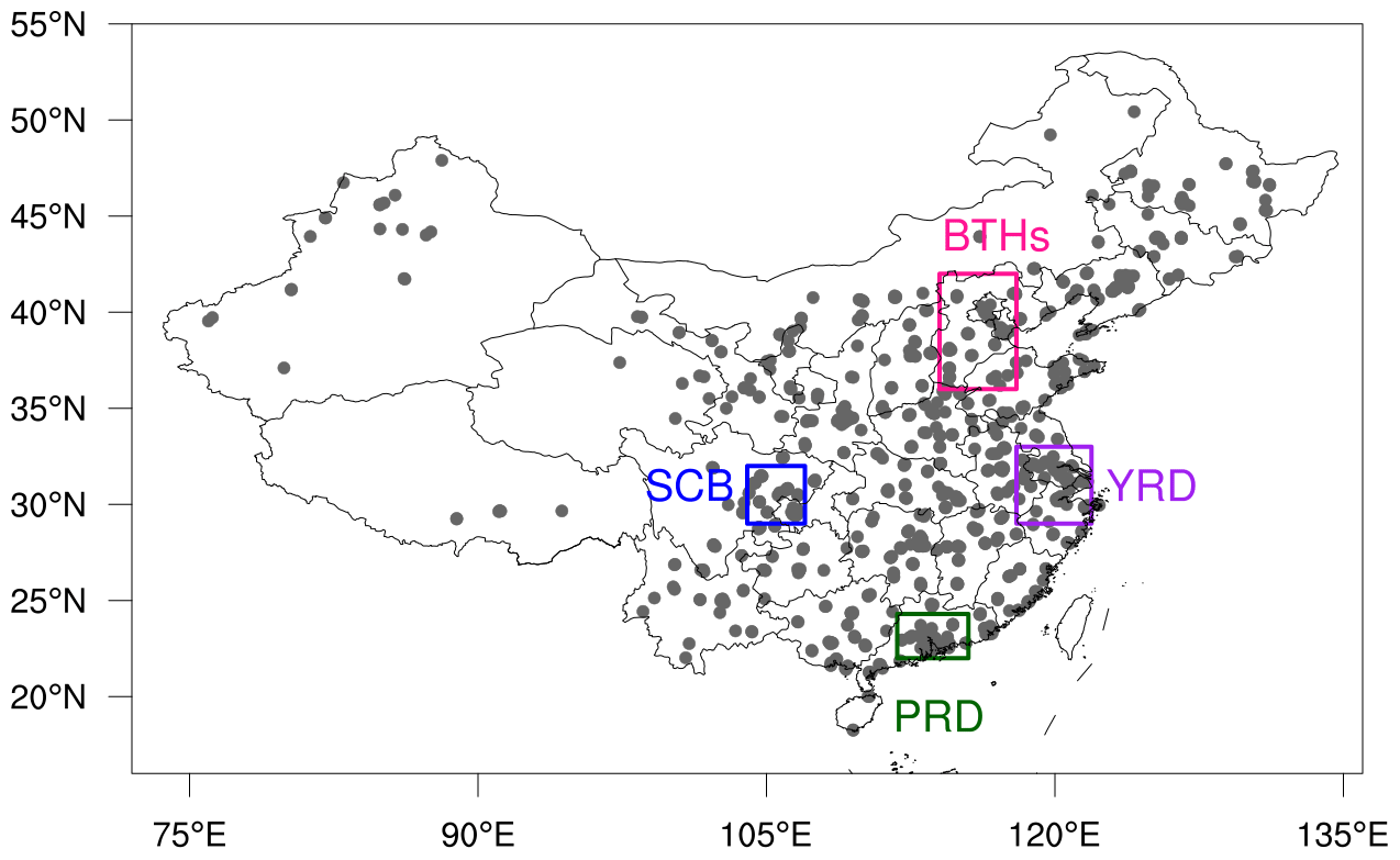
Figure 1 Study domain and locations of the selected monitoring sites. The pink, blue, purple, and green rectangles indicate Beijing–Tianjin–Hebei and its surroundings (BTHs) as well as the Sichuan Basin (SCB), Yangtze River Delta (YRD), and Pearl River Delta (PRD) regions, respectively.

The surface meteorological fields used in this study include sea surface pressure, horizontal wind at 10 m, air temperature at 2 m, downward solar radiation, surface albedo, and total precipitation. The variables selected at 850 and 100 hPa include relative humidity as well as horizontal and vertical velocity. These meteorological variables have been shown by many previous studies to correlate strongly with surface O₃ concentrations as discussed above. Hourly reanalysis data for meteorological variables were obtained from the fifth-generation European Centre for Medium-Range Weather Forecasts (ECMWF) reanalysis dataset (ERA5) with a spatial resolution of $\mathrm{0.25}{}^{\circ }\times \mathrm{0.25}{}^{\circ }$ from 1981 to 2019 (https://cds.climate.copernicus.eu/, last access: 24 December 2023). This spatial resolution sets the highest limit of resolution for our hybrid O₃ product.

The national land use data with a spatial resolution of 1 km × 1 km for 2013 were obtained from the Resource and Environment Science data center of the Chinese Academy of Sciences (RESDC) (http://www.resdc.cn, last access: 24 December 2023). Six primary types of land use are considered: cultivated land, forestland, grassland, water bodies, construction land, and unused land. Nationwide elevation data were also provided by the RESDC (https://www.resdc.cn/data.aspx?DATAID=123, last access: 24 December 2023), which are resampled based on the latest Shuttle Radar Topography Mission (SRTM) v4.1 data developed in 2000.

The spatial distribution of the harvested areas for four staple crops (wheat, rice, maize, soybean) in China was obtained from the Global Agro-Ecological Zones 2015 dataset (https://doi.org/10.7910/DVN/KJFUO1). Crop harvesting dates with a resolution of $\mathrm{0.5}{}^{\circ }\times \mathrm{0.5}{}^{\circ }$ were provided by the Center for Sustainability and the Global Environment (Sacks et al., 2010). For crops having more than one growing season in a year, only the primary growing period was considered.

2.2 GEOS-Chem model

We used the GEOS-Chem global 3-D chemical transport model version 12.2.0 (https://geoschem.github.io/, last access: 24 December 2023), driven by assimilated meteorological data from Modern-Era Retrospective analysis for Research and Applications, version 2 (MERRA2) (https://gmao.gsfc.nasa.gov/reanalysis/MERRA-2/, last access: 24 December 2023) with a horizontal resolution of 2.0^∘ latitude by 2.5^∘ longitude and reduced vertical resolution of 47 levels. GEOS-Chem incorporates meteorological conditions, emissions, chemical information, and surface conditions to simulate the formation, transport, mixing, and deposition of ambient O₃. It performs fully coupled simulations of O₃–NO_x–VOC–aerosol chemistry (Bey et al., 2001). Previous studies have demonstrated the ability of GEOS-Chem to reasonably reproduce the magnitudes and seasonal variations of surface O₃ in eastern Asia (Wang et al., 2011; He et al., 2012). To provide long-term simulated O₃ fields for incorporation into the ML model (see below), we conducted GEOS-Chem simulations at a resolution of $\mathrm{2.0}{}^{\circ }\times \mathrm{2.5}{}^{\circ }$; higher resolutions of GEOS-Chem in nested grids are available but computationally prohibitive for multidecadal simulations. The original unit of GEOS-Chem-simulated O₃ is parts per billion (ppb), which was converted to micrograms per cubic meter (µg m⁻³) assuming a constant temperature of 25 ^∘C and pressure of 1013.25 hPa (1 µg m⁻³ is approximately 0.5 ppb) when compared with observations (P. Yin et al., 2017; Gong and Liao, 2019).

Global anthropogenic emissions of CO, NO_x, SO₂, and VOCs are from the Community Emissions Data System (CEDS), which has coverage over the simulation years of 1950–2014 (Hoesly et al., 2018). Biomass burning emissions are from the Global Fire Emissions Database (GFED4) inventory (van der Werf et al., 2017). Biogenic VOC emissions are computed by the Model of Emissions of Gases and Aerosols from Nature (MEGAN) v2.1 (Guenther et al., 2012), which is embedded in GEOS-Chem. Emissions of biogenic VOC species in each grid cell, including isoprene, monoterpenes, methyl butanol, sesquiterpenes, acetone, and various alkenes, are simulated as a function of canopy-scale emission factors modulated by environmental activity factors to account for changing temperature, light, leaf age, leaf area index (LAI), soil moisture, and CO₂ concentrations (Sindelarova et al., 2014).

Dry deposition follows the resistance-in-series scheme of Wesely (1989), which depends on species properties, land cover types, and meteorological conditions, and uses the Olson land cover classes with 76 land types reclassified into 11 land types. Although transpiration is a potential mechanism via which the land cover affects ozone, we do not address it in this study because water vapor concentration in GEOS-Chem is prescribed from assimilated relative humidity (i.e., not computed online from evapotranspiration).

2.3 LightGBM machine learning model

The primary purpose of utilizing ML here was to minimize the biases of model output as compared with observations, whereby the biases could arise from incomplete model physics, input and parameter errors, numerical errors, coding errors, and representation errors (i.e., mismatch in spatial scales between model grid cells and site observations), so that the output of the hybrid model could have the closest values to the observations and enable more accurate impact evaluation. In this study, we used the LightGBM ML algorithm to integrate GEOS-Chem-simulated O₃ at a lower resolution with higher-resolution multi-source data to produce higher-resolution hourly O₃ and MDA8 O₃ fields.

LightGBM is a ML algorithm based on the gradient-boosting decision tree (Chen and Guestrin, 2016), which has a high training efficiency and lower memory footprint and is thus suitable for processing massive high-dimensional data (Zhang et al., 2019). The general steps to build a ML model can be summarized as follows: (1) choose an algorithm that is appropriate for the problem (e.g., regression or classification), (2) clean the data and split them into training and test data, (3) train and tune the model with training data to capture prediction patterns well, (4) evaluate the model performance on test data, and (5) return to step (3) and (4) until an optimal predictive ability is reached. The training and evaluation processes are both performed at the site level in accordance with the observations, whereby the predictor variables and model responses were first sampled at the same locations using the bilinear interpolation approach (Accadia et al., 2003). This approach of handling spatial-scale mismatch between model grid cells and site observations has been commonly used in previous studies (e.g., Li et al., 2021). When predicting the gridded O₃ concentrations with the trained model, predictor variables at different spatial resolutions were all regridded to the same resolution of $\mathrm{0.25}{}^{\circ }\times \mathrm{0.25}{}^{\circ }$, consistent with the ERA5 meteorological fields. By taking advantage of these higher-resolution datasets, the hybrid approach can not only correct the biases of the GEOS-Chem-simulated O₃, but also refine them into a finer resolution. To evaluate if the hybrid approach truly benefits from using higher-resolution meteorological fields, we also repeated the whole training exercise with the input meteorology of GEOS-Chem (MERRA2 at $\mathrm{2.0}{}^{\circ }\times \mathrm{2.5}{}^{\circ }$) instead of ERA5.

During the model training process, the model was evaluated with 10-fold cross-validation to ensure the robustness and reliability of the model, whereby the training data were randomly partitioned into 10 subsets of approximately the same size, with 90 % of the data used to train individual models and the ensemble model and the remaining 10 % of data used to examine model performance (Xiao et al., 2018). This process was repeated 10 times so that each data record was left for testing once. The tuning of the hyperparameters was optimized using grid search optimization to improve detection performance and diagnostic accuracy (Wang et al., 2019). Statistical indicators, including the coefficient of determination (R²) and root mean square error (RMSE), were used in a subsequent assessment of model performance for GEOS-Chem alone and for the hybrid approach.

Our analysis revealed that training the model with 1 year or more of data results in only marginal reductions in RMSE and enhancements in R² (Fig. S1 in the Supplement); thus a timescale of 2 years appears to strike a good balance between computational burden and model accuracy. These results align with the findings of Ivatt and Evans (2020), who suggested that much of the variability in the power spectrum of surface O₃ can be captured by timescales of a year or less. Therefore, here we utilized observations from the 2016–2017 period as the training data, which offered a more economical computing cost and improved training time efficiency, and observations in 2018 as the independent test data to evaluate model performance.

2.4 Ozone-exposure metric and exposure–yield response functions

Among O₃-exposure indices, AOT40 has been widely used during the last 2 decades as it has been found to have a strong relationship with the relative yield of many crop species (Mills et al., 2007) and was thus used to quantify the impacts of surface O₃ on crop yields in this study. The flux-based metrics, which require long-term simulations using a process-based stomatal uptake model, were beyond the scope of this study. The AOT40 (ppm-h) is defined as follows:

$$\begin{array}{}\text{(1)}& \mathrm{AOT}\mathrm{40}=\sum _{i=\mathrm{1}}^n\left({\left[{\mathrm{O}}_{\mathrm{3}}\right]}_i-\mathrm{0.04}\right),\end{array}$$

where [O₃]_i is the hourly mean O₃ concentration (ppm) during the 12 h of local daytime (08:00–19:59 LT), and n is the number of hours in the growing season defined as the 90 d prior to the start of the harvesting period according to the crop calendar.

The exposure–yield response functions based on extensive field experimental studies have been established to relate a quantifiable O₃-exposure metric to crop yields. It has been suggested that responses of crop yields were found to be greater in Asian experiments than in the American and European counterparts, indicating possibly higher O₃ sensitivity of Asian crop varieties (Emberson et al., 2009; Feng et al., 2022). To better understand O₃-induced risks to crops in China, the AOT40 exposure–yield functions developed based on field experiments in China are used in this study, which are named AOT40-China. The exposure–yield response functions for soybean are from Zhang et al. (2017), and those of the other three crops are from Feng et al. (2022). The statistical exposure–yield relationships used in this study are summarized in Table S1 in the Supplement.

2.5 Analysis of health impacts

All-cause mortality, cardiovascular disease mortality, and respiratory disease mortality are selected as the health outcomes of our study due to the high correlation between these endpoints and short-term O₃ exposure found in previous studies. A log-linear exposure–response function is widely adopted and recommended by the World Health Organization (WHO) for health impact assessment in areas with severe air pollution. In particular, the log-linear model is the most widely applied exposure–response model at present in China (Lelieveld et al., 2015; H. Yin et al., 2017; Zhang et al., 2022b). The premature mortality is calculated following

$$\begin{array}{}\text{(2)}& \mathrm{\Delta }M=\mathit{\delta }c\cdot \left[{\displaystyle \frac{(\mathrm{RR}-\mathrm{1})}{\mathrm{RR}}}\right]\cdot P,\end{array}$$

where ΔM is the excess mortality attributable to O₃ exposure, δc is the baseline mortality rate for a particular health endpoint (P. Yin et al., 2017; Madaniyazi et al., 2016), P is the exposed population, and RR is the relative risk defined as

$$\begin{array}{}\text{(3)}& \mathrm{RR}=\exp \left(\left(X-X_{\mathrm{0}}\right)\cdot \mathit{\beta }\right).\end{array}$$

Here, β is the exposure–response coefficient derived from epidemiological cohort studies (Shang et al., 2013), X represents the model-calculated O₃ concentration, and the value of X₀ is the threshold concentration below which no additional risk is assumed. Consistent with previous studies (Lelieveld et al., 2015; Liu et al., 2018), we used X₀=75.2 µg m⁻³.

In this study, the mean MDA8 O₃ concentrations in warm seasons (May–September) were used to estimate the disease-specific health impacts of short-term exposure to O₃. The province-level population and national baseline mortality rate for particular diseases were provided by the National Bureau of Statistics (https://www.stats.gov.cn/english/, last access: 24 December 2023). The spatial differences of baseline mortality in China were not considered without provincial-level data, which means that we assume the baseline mortality is evenly distributed across China (Dedoussi et al., 2020). The exposure–response coefficients were obtained from existing epidemiological studies in China (Table S2). If the corresponding coefficient of a province could not be found in published epidemiological studies, the datum closest to that province would be selected as a substitute. If there were no neighboring provinces, the results of national meta-analysis was used (Zhang et al., 2021).

3 Results

3.1 Model development and validation

The final selected features and their importance estimated by the LightGBM algorithm based on 10-fold cross-validation are shown in Fig. 2. GEOS-Chem-simulated O₃ is the top predictor of surface O₃ concentrations, accounting for 61 % and 58 % of all relative importance in the ML algorithm predicting hourly O₃ and daily MD8A-O₃, respectively. The result indicates that process-based GEOS-Chem simulations have high utility for O₃ predictions under the hybrid approach (Ma et al., 2021). The meteorological variables with a high contribution to both the daily and the hourly models are downward surface solar radiation (SSRD), relative humidity at 1000 hPa (RH_1000hpa), and 10 m horizontal wind (U₁₀ and V₁₀). Other special features, including location (latitude and longitude), elevation, and diurnal and monthly patterns of O₃, also contribute to ambient O₃ estimations. The spatial distributions of bias-corrected O₃ are consistent with observations for both training and test datasets (Fig. S2), indicating that there is no obvious overfitting; i.e., the model is able to generalize from the training set to the test set. The good generalization ability of the model gives us confidence in its ability to make accurate predictions based on new data. In general, the hybrid approach can yield good O₃ estimates in the data-intensive regions, including eastern and central China, which are the hotspot areas of O₃ pollution.

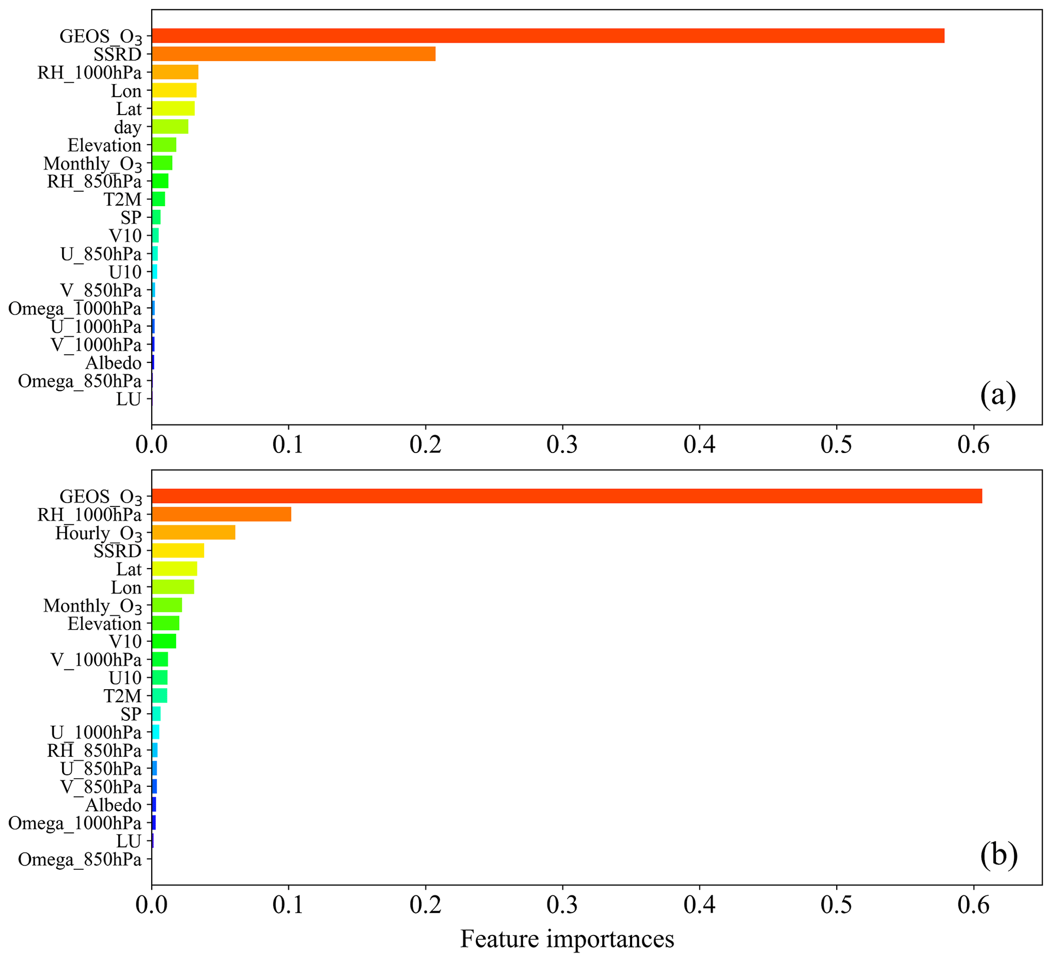
Figure 2 The feature importance plot for (a) MDA8 O₃ and (b) hourly O₃. The full list of candidate variables with their symbols, units, descriptions, and data sources are shown in Table S3.

Figure 3 shows the density scatterplots between O₃ measurements and GEOS-Chem simulations, as well as the hybrid approach predictions for 2018. The R² values of the hybrid approach and GEOS-Chem model are 0.66 and 0.27 at the hourly level and 0.72 and 0.53 at the MDA8 O₃ level, respectively. Bias-corrected O₃ concentrations have lower RMSEs in comparison with GEOS-Chem-simulated O₃ concentrations, reduced from 31.1 to 23.8 µg m⁻³ for MDA8 O₃ predictions and from 38.5 to 26.3 µg m⁻³ for hourly predictions. The MDA8 O₃ model performance is better than that of the hourly model, indicating reduced errors upon temporal averaging. To test if using the higher-resolution meteorological data offers better prediction accuracy compared with the original input meteorology of GEOS-Chem, the MERRA2 dataset driving GEOS-Chem was also used to train the model. We found that the higher-resolution ERA5 dataset performed better in reproducing observed O₃ concentrations with moderately smaller RMSEs and larger R² values (Fig. S3), demonstrating the extent to which a higher-resolution meteorological dataset, despite not being strictly consistent with the input meteorology for the CTM, can help enhance the performance of the hybrid approach and help resolve finer spatial details within the original CTM grid cells. In summary, the result suggests that the CTM-simulated results can be substantially improved by applying ML with multi-source datasets, and the bias-corrected data can improve our understanding of long-term O₃ trends and its further implications on crop and human health over China, as discussed in the following sections.

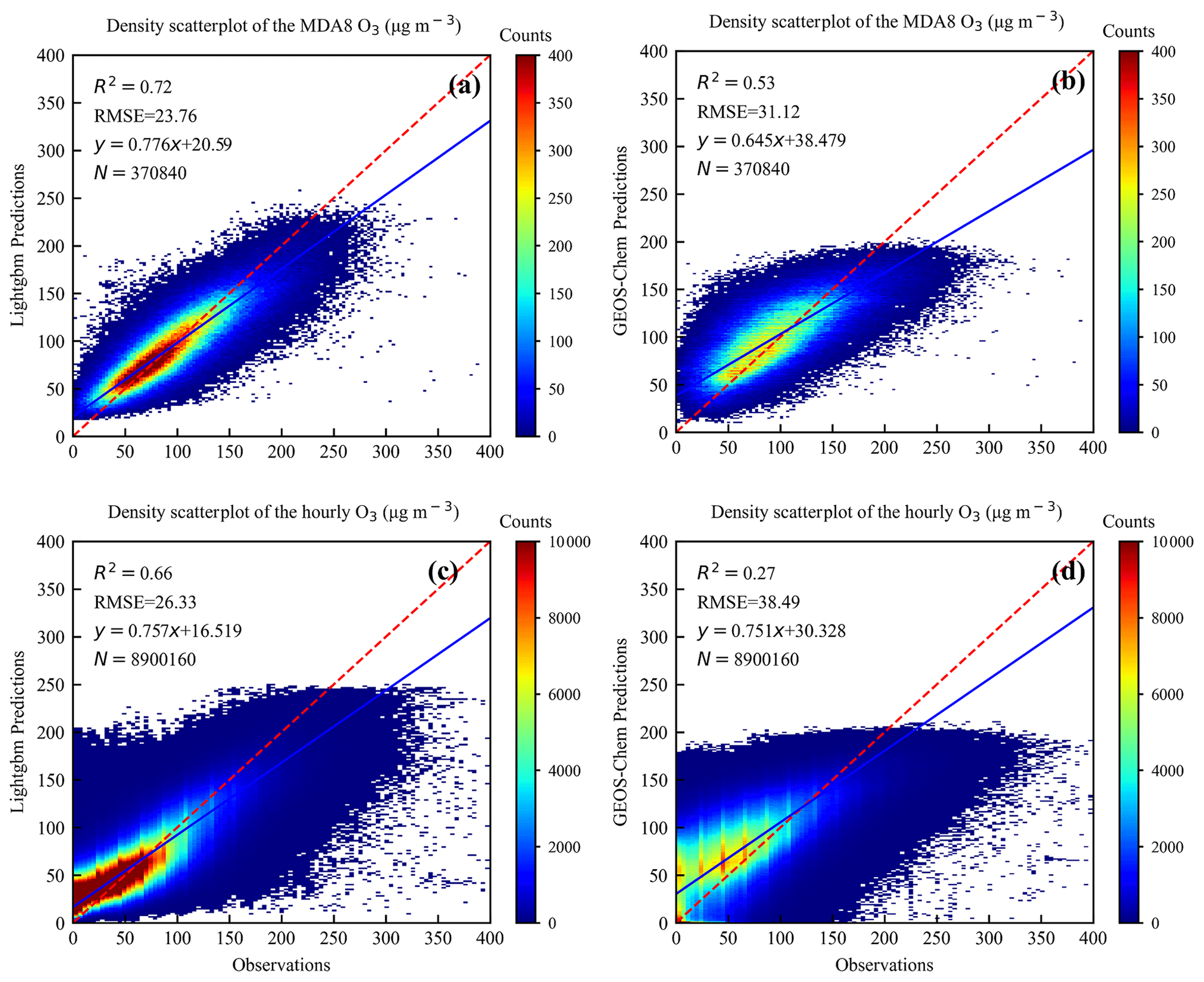
Figure 3 Density scatterplots and linear regression statistics of O₃ predictions vs. observations for 2018: (a) bias-corrected MDA8 O₃ vs. observations, (b) GEOS-Chem MDA8 O₃ vs. observations, (c) bias-corrected hourly O₃ vs. observations, and (d) GEOS-Chem hourly O₃ vs. observations. The model results are sampled at the same locations. The dashed red line indicates the 1:1 line, and the solid blue line indicates the line of best fit using orthogonal regression. R² is the coefficient of determination, RMSE is the root mean square error, and N is the number of data points. The x and y axes represent the O₃ observations and predictions, respectively.

In comparison with previous studies, Liu et al. (2020) used XGBoost to predict O₃ in major urban areas of China at a resolution of $\mathrm{0.1}{}^{\circ }\times \mathrm{0.1}{}^{\circ }$, and the R² value and RMSE for MDA8 O₃ were 0.74 and 23.8 µg m⁻³, respectively. Their result indicates that higher-resolution predictions may help enhance model accuracy but represent a trade-off between model accuracy and time efficiency, depending on the purpose. Instead of directly predicting O₃ concentrations, Ivatt and Evans (2020) predicted biases in GEOS-Chem-simulated O₃ concentrations and then corrected them with XGBoost. They also suggested that the corrected model performs considerably better than the uncorrected model, with RMSE reduced from 32.4 to 15.0 µg m⁻³ and Pearson's R raised from 0.48 to 0.84. Their greater improvement with larger reduced RMSE than our result is mainly because they selected fewer sites for training, with all the urban and mountain sites (observations made at a pressure < 850 hPa) removed. The removal of these sites can improve the overall apparent performance of the model because O₃ formation could have different characteristics in these areas. In general, ML methods have been proven to be a promising tool to improve air pollutant forecasts when a process-level understanding is still incomplete.

3.2 Spatiotemporal distribution and trends in O₃ predictions

Figure 4 demonstrates the spatial patterns of averaged annual and warm-season (May–September) MDA8 O₃ from 1981 to 2019. When compared to the high concentrations in the warm season, MDA8 O₃ concentrations are relatively lower at an annual level. The annual and warm-season MDA8 O₃ concentrations have similar spatial distributions, and both present an increasing trend over the past few decades, with more substantial increases observed between 1981 and 2010. The O₃ levels in southern China are lower than those in northern China, but they are still relatively high in the PRD region, which is consistent with findings in previous studies (e.g., Liu and Wang, 2020a). During the first decade of 1981–1990, high-O₃-concentration areas are mainly concentrated in the BTHs and northern Shandong. In the next 2 decades, O₃ pollution expands extensively to most of eastern and northern China, spreading northward to Jilin and Liaoning; westward to Shanxi and Ningxia; and southward to northern Hunan, Shanxi, and Zhejiang. Moreover, the SCB and PRD regions also experience aggravated O₃ pollution during this period. In the last decade of the study period, O₃ concentrations remain at high levels in BTHs and SCB without obvious changes. Next we analyze the interannual variability to understand the detailed changes and trends in O₃.

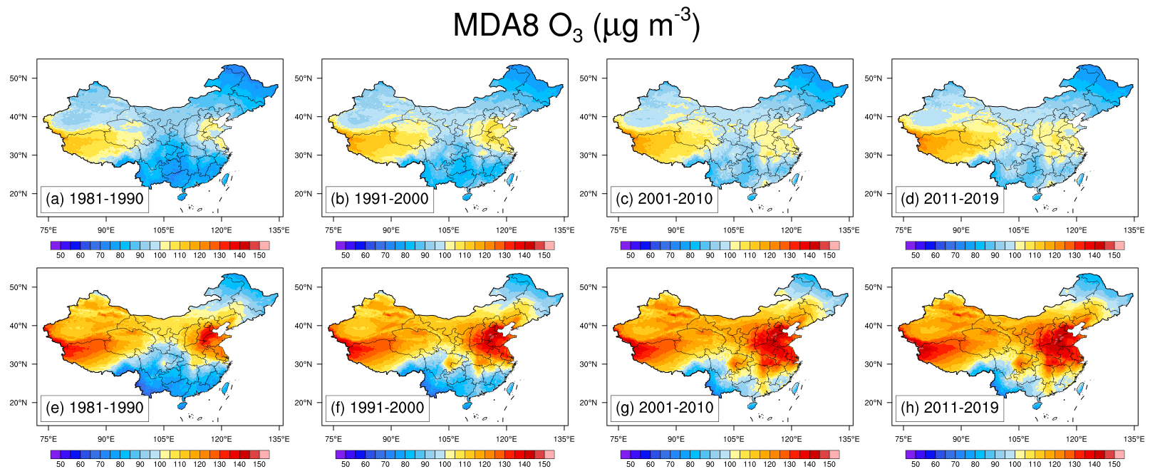
Figure 4 Spatial distribution of the annual mean MDA8 O₃ concentrations (µg m⁻³) during (a) 1981–1990, (b) 1991–2000, (c) 2001–2010, and (d) 2011–2019. Spatial distribution of the warm-season (May–September) mean MDA8 O₃ concentrations of (e) 1981–1990, (f) 1991–2000, (g) 2001–2010, and (h) 2011–2019.

Figure 5 shows that the annual averaged MDA8 O₃ concentrations increased from 87 µg m⁻³ in 1981 to 98 µg m⁻³ in 2019, with a growth rate of +0.26 µg m⁻³ yr⁻¹, while the warm-season averaged MDA8 O₃ concentrations increased from 100 µg m⁻³ in 1981 to 117 µg m⁻³ in 2019, having a growth rate of +0.51 µg m⁻³ yr⁻¹. Moreover, the average annual and warm-season O₃ concentrations have a more obvious upward trend before the 2000s, with a growth rate of 0.38 and 0.71 µg m⁻³ yr⁻¹, compared to that after the 2000s, when O₃ concentrations appear to fluctuate within a certain range. GEOS-Chem-simulated O₃ has a similar trend to the bias-corrected O₃, but it generally overestimates O₃ concentrations on a national scale (Fig. S4). The annual and warm-season averaged MDA8 O₃ concentrations in BTHs as well as the YRD, SCB, and PRD regions are shown in Figs. S5 and S6. The warm-season increasing trends for BTHs as well as the YRD, SCB, and PRD regions are 0.32, 0.63, 0.84, and 0.81 µg m⁻³ yr⁻¹ from the years 1981 to 2019.

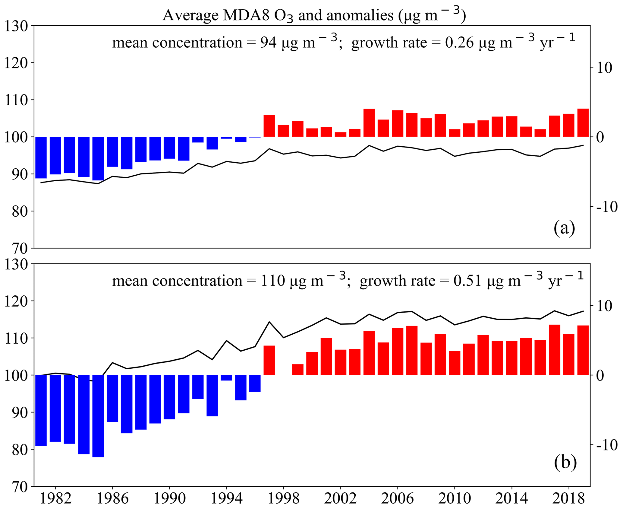
Figure 5 The bias-corrected MDA8 O₃ predictions (black line; upper y axis) and corresponding anomalies (colored bar; lower y axis) from 1981 to 2019: (a) annual mean and (b) warm-season mean (May–September). The trends (growth rates) are obtained through ordinary linear regression on mean values of MDA8 O₃. The anomalies are defined as the annual mean minus the multidecadal average over 1981–2019.

In recent years, the worsening O₃ pollution has fueled numerous studies on ground-level O₃ spatial distribution and changes in China, which have been conducted on local, regional, and national scales using different O₃ fields from observations, CTMs, and ML estimates. In this study, we mainly focus on the regional and national O₃ characteristics, and the O₃ trends reported in recent studies are listed in Table 1. By comparing the results of existing works, we find that source-varied O₃ fields can induce great uncertainty in the O₃ trends. Moreover, the O₃ trends are found to be very sensitive to the study period even with the same O₃ fields (Wei et al., 2022), which indicates large interannual variability, mostly reflecting the changing anthropogenic emissions and meteorology (Lu et al., 2019; Li et al., 2020). In contrast to the perceptible O₃ trends, Liu et al. (2020) suggested that O₃ pollution in most parts of China undergoes only modest changes between 2005 and 2017, and their trends were not spatially continuous. T. Wang et al. (2022) also reported that O₃ has small positive increase rates for 2013–2021 in many cities, and the O₃ increase rates greatly differ from site to site even within the same region.

Table 1 Summary of reported regional and national MDA8 O₃ trends (µg m⁻³ yr⁻¹).

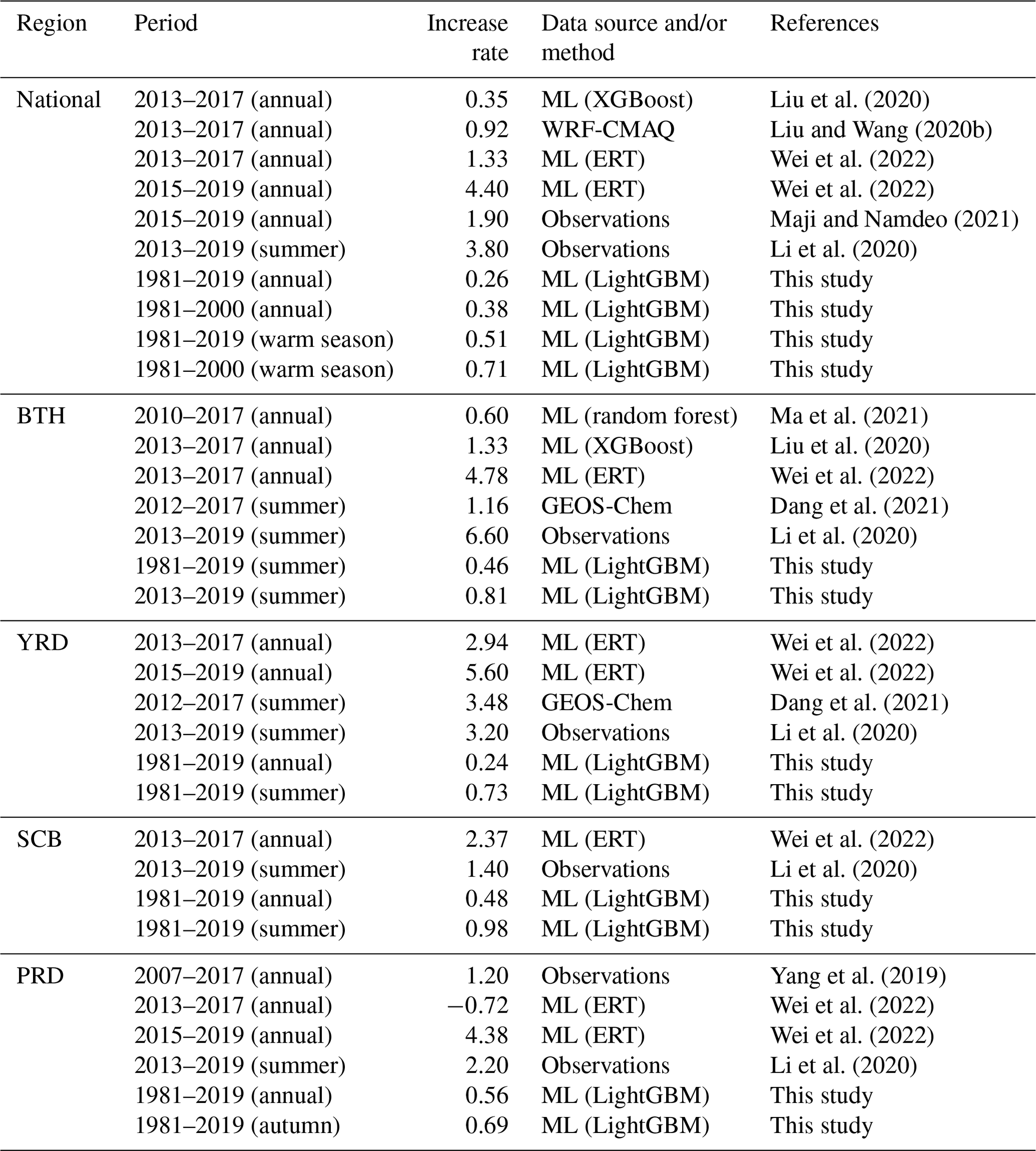
In comparison, our results indicate no obvious increasing trends in national MDA8 O₃ within the same study period. On a regional scale, only BTHs have a perceptible increasing trend in more recent years, while no such trends are found over the YRD, SCB, and PRD regions during the same period. The summertime MDA8 O₃ in BTHs has a change rate of +0.81 µg m⁻³ yr⁻¹, which is much lower than the results using O₃ observations (Li et al., 2020). One possible reason is that most observational sites are in urban regions, which usually suffer more serious O₃ pollution, while the O₃ concentrations from model simulations and ML methods are calculated on the scale of a grid cell with lower domain-averaged values. Moreover, gridded data at a relatively coarse resolution may fail to capture larger site differences, leading to the larger discrepancy between O₃ observations and gridded O₃ estimates.

3.3 Seasonal characteristics of O₃ predictions

Differences in averaged annual and warm-season O₃ concentrations indicate that O₃ has distinctive seasonal characteristics. Figure 6 shows the seasonal variations in O₃ concentrations from 2011–2019, and results for the other past 3 decades are shown in Figs. S7–S9. In winter, pollution is mainly concentrated in the coastal areas of southern China. In spring, O₃ pollution primarily occurs in eastern China and the southern part of Yunnan Province. O₃ pollution continues to worsen over eastern China in summer, particularly in BTHs, and further extends to SCB. The air quality in eastern and central China is greatly improved in autumn, while southern China experiences the most pollution in this period. In general, the peak and trough values of O₃ concentrations appear in summer and winter, respectively. However, O₃ concentrations are found to be minimum in summer and maximum in autumn over PRD, which is largely determined by the summer monsoon (Zhou et al., 2013; H. Wang et al., 2018). Figure S10 shows the seasonal averaged MDA8 O₃ concentrations in different regions from 1981 to 2019. In winter, O₃ concentrations do not experience much change across the four regions over the past few decades, staying mostly between 70–80 μg m⁻³. Moreover, wintertime O₃ concentrations after the 2000s are generally lower than those before the 2000s in BTHs, YRD, and SCB. In contrast, summertime O₃ concentrations increase dramatically over the four regions. In spring and autumn, O₃ concentrations have an increasing trend in PRD, while it mostly fluctuates within a certain range in the other three regions. The results show that O₃ in non-winter seasons has a more pronounced increase during 1981–2019 albeit with regional differences. The regional characteristics of O₃ and its influencing factors are further discussed in Sect. 3.4. BTHs as well as the SCB, YRD, and PRD regions have been identified as hotspots of O₃ pollution in China. These regions are characterized by high population density (L. Wang et al., 2018) and are also major agricultural areas (Monfreda et al., 2008), which may face greater burdens of crop yield and human health losses with high O₃ concentrations. Therefore, here we provide more detailed analysis and investigation of these regions.

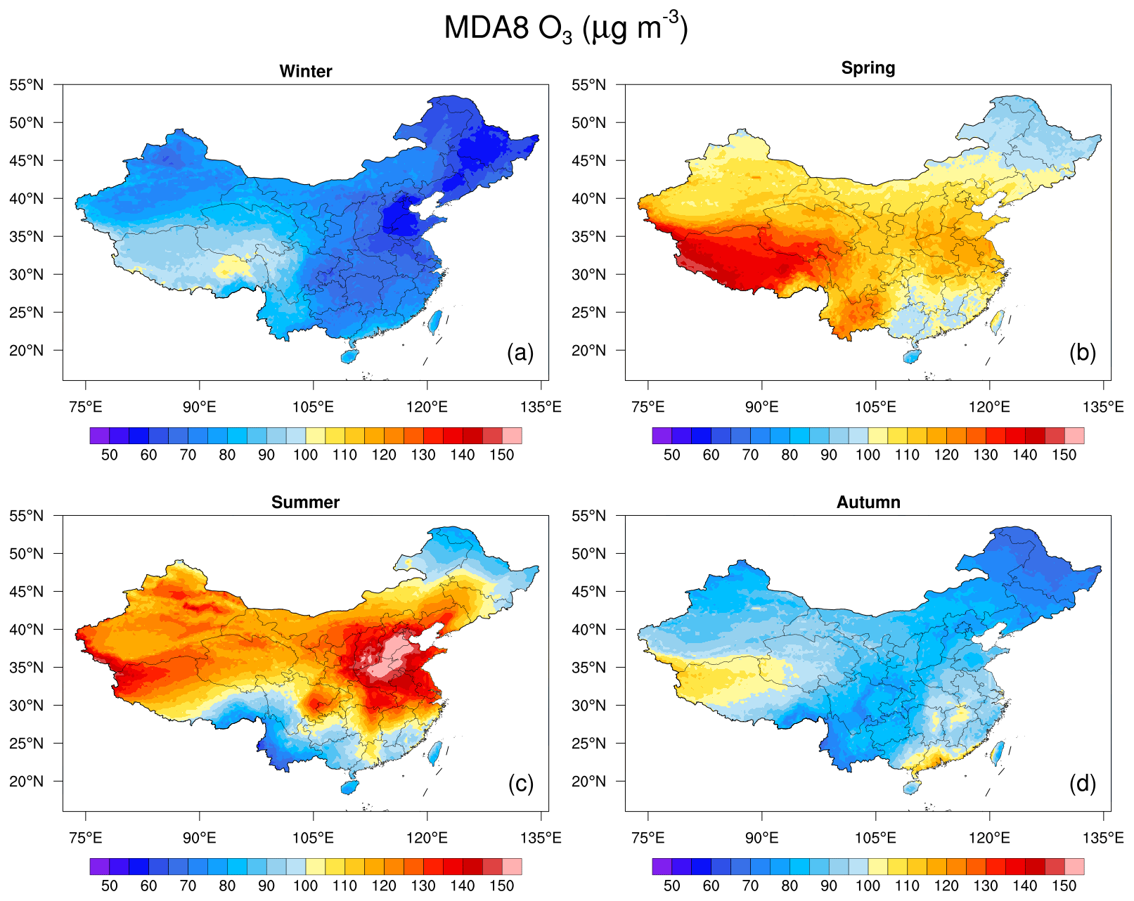
Figure 6 Spatial distribution of the bias-corrected MDA8 O₃ predictions (µg m⁻³) from 2011–2019: (a) winter, (b) spring, (c) summer, and (d) autumn.

3.4 Regional characteristics of O₃ predictions

Figure 7 shows the bar plots of the seasonal MDA8 O₃ concentrations in each region from 1981–2019 for bias-corrected and GEOS-Chem-simulated O₃. For the bias-corrected O₃, the averaged summertime MDA8 O₃ concentrations in BTHs, YRD, and SCB and autumn-time MDA8 O₃ concentrations in PRD are 137±8, 119±10, 113±12, and 98±10 µg m⁻³, with the increasing rate being 0.46, 0.73, 0.98, and 0.69 µg m⁻³ yr⁻¹ from 1981 to 2019, respectively (Fig. S11). For GEOS-Chem-simulated O₃, the averaged summertime MDA8 O₃ concentrations in BTHs, YRD, and SCB and autumn-time MDA8 O₃ concentrations in PRD are 141±7, 125±11, 120±14, and 100±12 µg m⁻³, respectively. This shows that O₃ concentrations of the four regions have a consistent upward trend in the summer over the past few decades, but there are regional differences in other seasons. Compared to BTHs and YRD, PRD and SCB have more distinctive O₃ increases in spring and autumn. Among these four regions, the O₃ concentrations have the biggest seasonal differences in BTHs and the smallest seasonal differences in PRD.

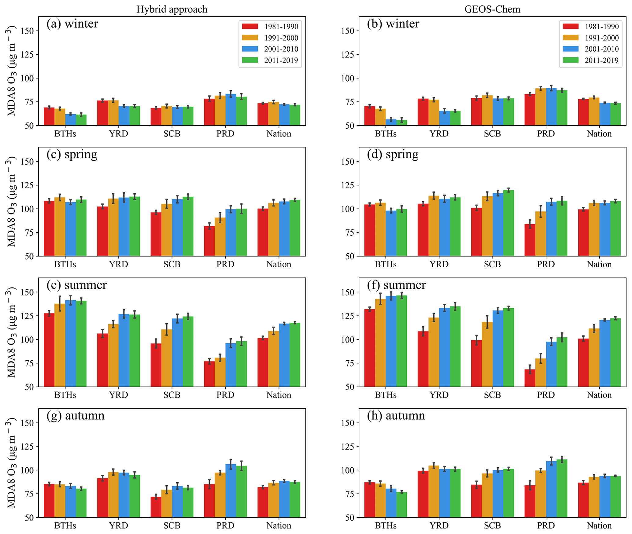
Figure 7 The seasonal mean MDA8 O₃ concentrations (µg m⁻³) in different regions during 1981–2019. Bias-corrected MDA8 O₃ in (a) winter, (c) spring, (e) summer, and (g) autumn. GEOS-Chem MDA8 O₃ in (b) winter, (d) spring, (f) summer, and (h) autumn. The error bar represents the standard deviation.

The spatiotemporal patterns of O₃ in China have been proven to largely depend on both emissions and meteorology. The regional O₃ pollution is usually found to be triggered by specific circulation patterns as local meteorological factors are modulated by synoptic-scale circulation patterns. China has a large territory and is affected by different weather systems. The continental high-pressure systems, components of the eastern Asian summer monsoon (EASM) and tropical cyclones, among others, are critical synoptic conditions leading to O₃ formation and transport in China (T. Wang et al., 2022; Han et al., 2020). For instance, regional O₃ pollution in northern China usually occurs under a typical weather pattern of an anomalous high-pressure system at 500 hPa (Gong and Liao, 2019), which creates favorable meteorological conditions for high O₃ levels with high temperature, low relative humidity, anomalous southerlies, and divergence in the lower troposphere. As one of the most important components of EASM, the western Pacific subtropical high (WPSH) strongly influences summertime precipitation and atmospheric conditions in eastern China. A strong WPSH can decrease O₃ levels over YRD as enhanced moisture is transported into YRD under prevailing southwesterly winds (Zhao and Wang, 2017). Located on the southern coast of China, PRD features a typical subtropical monsoon climate. There, O₃ concentrations are usually the lowest in summer due to the prevailing southerlies with clean air from the ocean and the associated heavy rainfall, while the worst O₃ pollution usually happens in autumn, mainly due to the occasional northerly winds during the monsoonal transition, thereby importing precursors from the north, and stable and still relatively warm and sunny weather conditions before the winter starts. Downdrafts in the periphery circulation of a typhoon system can also strongly enhance surface O₃ before typhoon landing (Jiang et al., 2015; Lu et al., 2021; Li et al., 2022). On the one hand, the poor ventilation in the peripheral subsidence region of typhoons favors the accumulation of O₃ and its precursors. On the other hand, the deep subsidence can transport the O₃ in the upper troposphere and lower stratosphere to the surface, causing aggravated O₃ pollution. Moreover, smaller-scale circulation patterns, such as land–sea and mountain–valley breezes, also influence O₃ in coastal regions (Ding et al., 2004; Zhou et al., 2013; H. Wang et al., 2018).

When compared to the hybrid approach, GEOS-Chem generally has similar O₃ distribution and trends over each region, while overestimating O₃ concentrations (Table S4). GEOS-Chem particularly overestimates wintertime and autumn-time O₃ concentrations in SCB, which are 10±1 and 17±3 µg m⁻³ higher than those of the hybrid approach, respectively. Previous studies have reported such model overestimates and have proposed a number of explanations involving precursor emissions, dry deposition, and vertical mixing in the planetary boundary layer (PBL) (Lin et al., 2008; Travis et al., 2016; Fiore et al., 2005). Both observational analyses and inter-model comparisons suggested that the summertime dry deposition of O₃ calculated by the Wesely scheme in GEOS-Chem could be underestimated, which has been invoked as a cause for model overestimates of O₃. The biased emissions in the model, consistent with the biased-high tropospheric NO_x columns, result in overestimated O₃. Travis et al. (2016) showed that GEOS-Chem with reduced NO_x emissions provides an unbiased simulation of O₃ observations from aircraft and reproduces the observed O₃ production efficiency in the boundary layer. Lin et al. (2008) suggested that the excessive PBL mixing can lead to the biased-high O₃ concentrations. The fully mixed O₃ throughout the PBL means that the higher O₃ concentrations in the upper PBL are brought down to the surface much more efficiently. Moreover, the excessive spatial averaging of emissions at coarser resolutions could also lead to systematic overestimation of regional O₃ production (Wild and Prather, 2006). In summary, with a higher prediction accuracy, the hybrid approach lends greater credence to using model simulations to extrapolate historical O₃ further back in time, which can furthermore provide us with more accurate estimates of the impacts of O₃ on crop production and human health.

Figure 8 Estimated annual mean relative yield losses (RYLs; in %) of four staple crops from 1981–2019 using the AOT40-China metric. The estimated RYLs using bias-corrected O₃ for (a) maize, (d) wheat, (g) soybean, and (j) rice. The estimated RYLs using GEOS-Chem-simulated O₃ for (b) maize, (e) wheat, (h) soybean, and (k) rice. The differences in estimated RYLs between GEOS-Chem-simulated and bias-corrected O₃ for (c) maize, (f) wheat, (i) soybean, and (l) rice. The GEOS-Chem-simulated O₃ was regridded to $\mathrm{0.5}{}^{\circ }\times \mathrm{0.5}{}^{\circ }$ for comparison with bias-corrected O₃.

3.5 Crop production losses attributable to O₃ pollution

Figure 8 shows the relative yield losses (RYLs; RYL = 1 − RY, where RY is the relative yield defined as the ratio of the O₃-affected yield to the yield without O₃ exposure) calculated with GEOS-Chem and bias-corrected O₃ using the AOT40-China metric. For a given crop, the RYLs show generally consistent spatial distribution across the metrics, with BTHs having the most serious crop yield losses due to high O₃ concentrations. Compared to the bias-corrected O₃, using GEOS-Chem-simulated O₃ generally leads to larger yield losses, especially over BTHs and SCB, reflecting overestimated O₃ concentrations by GEOS-Chem in cropland areas during the growing seasons (Fig. S12), primarily in spring and summer, which is consistent with the above analysis. GEOS-Chem-simulated O₃ leads to slightly underestimated wheat yield loss only over some parts of BTHs, mostly because the primary growing period of wheat there is in winter and spring, and GEOS-Chem has lower O₃ estimates than the hybrid approach during this period there (Table S4).

Figure 9 shows the bar plots of the relative yield for each crop using the AOT40-China exposure–yield response relationship. Crop yield losses are generally consistent with the O₃ trends as the exposure–yield relationships used here are essentially a set of linear functions. Most crops experience aggravated yield losses over the past 4 decades due to enhanced O₃ concentrations, except for wheat, which has the largest yield loss during the period from 1991 to 2000. The reason could be that BTHs have the highest O₃ concentrations in spring during the 1990s, which is the primary growing season for wheat (Fig. S13).

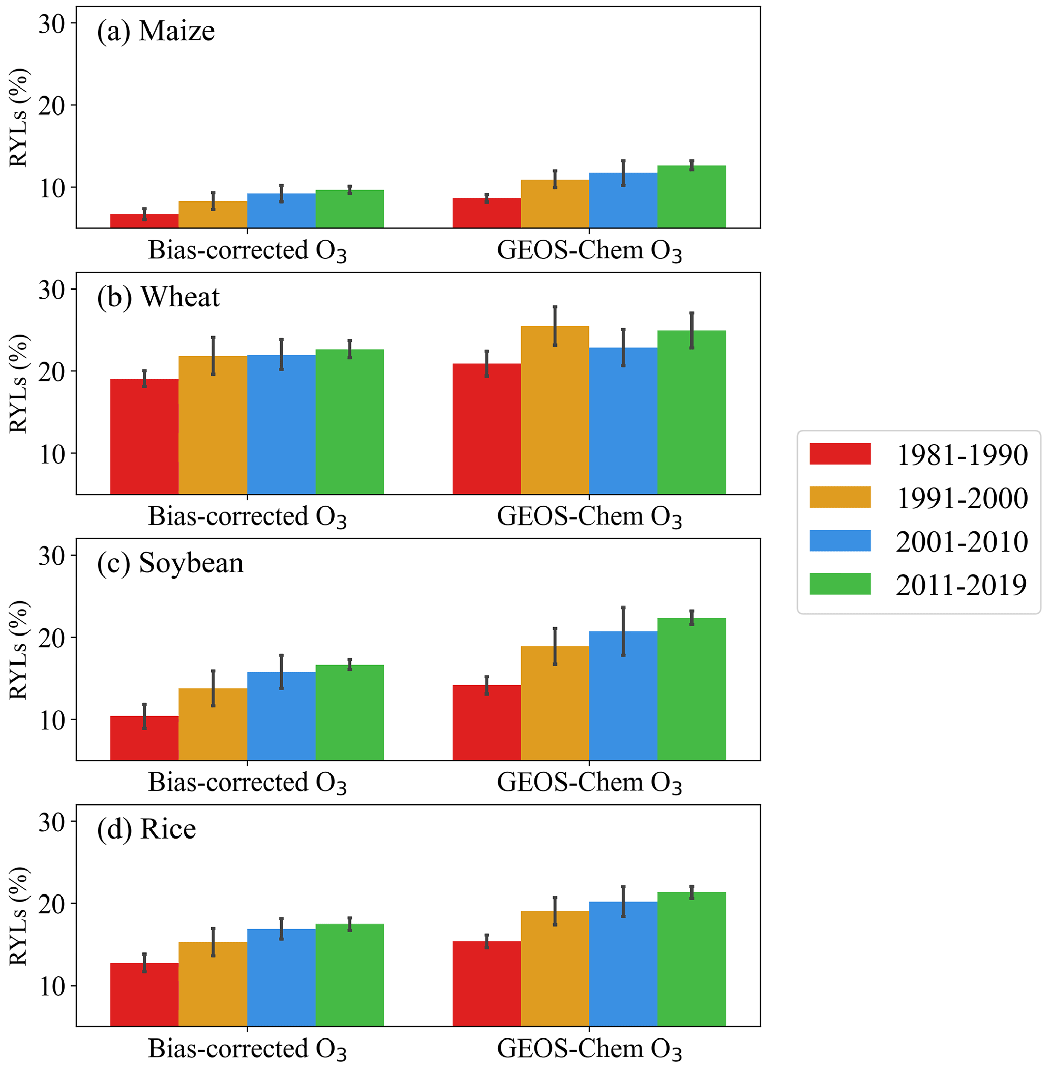
Figure 9 The estimated decadal mean relative yield losses (RYLs) of four staple crops using different metrics from 1981–2019. The estimated RYLs using bias-corrected O₃ and GEOS-Chem-simulated O₃ for (a) maize, (b) wheat, (c) soybean, and (d) rice. The error bar represents the standard deviation.

The average annual crop RYLs from 1981 to 2019 for wheat, rice, soybean, and maize range from 1.1 % to 13.4 %, 2.7 % to 13.4 %, 6.3 % to 24.8 %, and 0.8 % to 7.4 %, respectively. The differences in yield losses across crops reflect the dependence on crop-specific phenology and ecophysiology. The estimated annual RYLs using bias-corrected O₃ for wheat, rice, soybean, and maize from 1981 to 2019 range from 17.5 %–25.5 %, 10.7 %–19.1 %, 7.3 %–17.9 %, and 7.1 %–12.7 %, with a growth rate of 0.03 % yr⁻¹, 0.04 % yr⁻¹, 0.27 % yr⁻¹, and 0.13 % yr⁻¹. Wheat is the most sensitive crop to the O₃ concentrations, whereas maize is the least sensitive. Using GEOS-Chem-simulated O₃, the estimated annual RYLs for wheat, rice, soybean, and maize from 1981 to 2019 are 18.7 %–28.7 %, 14.0 %–22.0 %, 12.4 %–23.1 %, and 7.9 %–13.2 %, having a growth rate of 0.08 % yr⁻¹, 0.14 % yr⁻¹, 0.23 % yr⁻¹, and 0.11 % yr⁻¹. There are noticeable differences in crop yield estimates using the bias-corrected and GEOS-Chem O₃, again indicating the importance of the bias-corrected high-resolution O₃ data in related crop issues.

In existing studies evaluating the O₃-induced crop losses in China, which also use exposure–yield relationships derived from the experiments conducted in Asia, Zhang et al. (2017) reported that the ambient O₃ concentrations in northeastern China cause substantial annual yield loss of soybean ranging from 23.4 % to 30.2 % during 2013 and 2014, depending on the O₃ metric used (including AOT40, W126, SUM06, and a flux-based metric). Feng et al. (2022), using AOT40, indicated that the annual average RYLs of wheat, rice, and maize from 2017 to 2019 are 33 %, 23 %, and 9 %, respectively. Our correspondingly estimated RYLs for rice (18.0 %) and maize (10.0 %) are generally consistent with their results, while the RYLs for soybean (16.4 %) and wheat (23.4 %) are much lower than their estimates. Since we used the same exposure–yield response relationships as in their studies, the discrepancies are primarily attributed to the differences in the metrics used (only for soybean), O₃ fields, and the sensitivity of the crop to the changes in O₃ concentrations (Mukherjee et al., 2021; Feng et al., 2022; Mills et al., 2018). In Zhang et al. (2017), the O₃ measurements are obtained from the experimental field (45^∘73^′ N, 126^∘61^′ E), and in Feng et al. (2022), the measured O₃ concentrations are from over 3000 monitoring sites across eastern Asia. The results of the comparison are consistent with the previous analysis of O₃ trends and variability from different sources, where the domain-averaged values of O₃ observations are larger than gridded O₃ from model simulations (Sect. 3.2) and thus lead to larger estimates of RYLs. On the one hand, it indicates that O₃ fields should be considered a great source of uncertainty when comparing the results of previous studies using source-varied O₃ fields. Moreover, different degrees of importance should be given for specific crops; for example, the changes in O₃ concentrations have a larger impact on wheat crop. On the other hand, it again highlights the necessity and importance of bias correction for model-simulated O₃ when studying O₃-induced crop reduction.

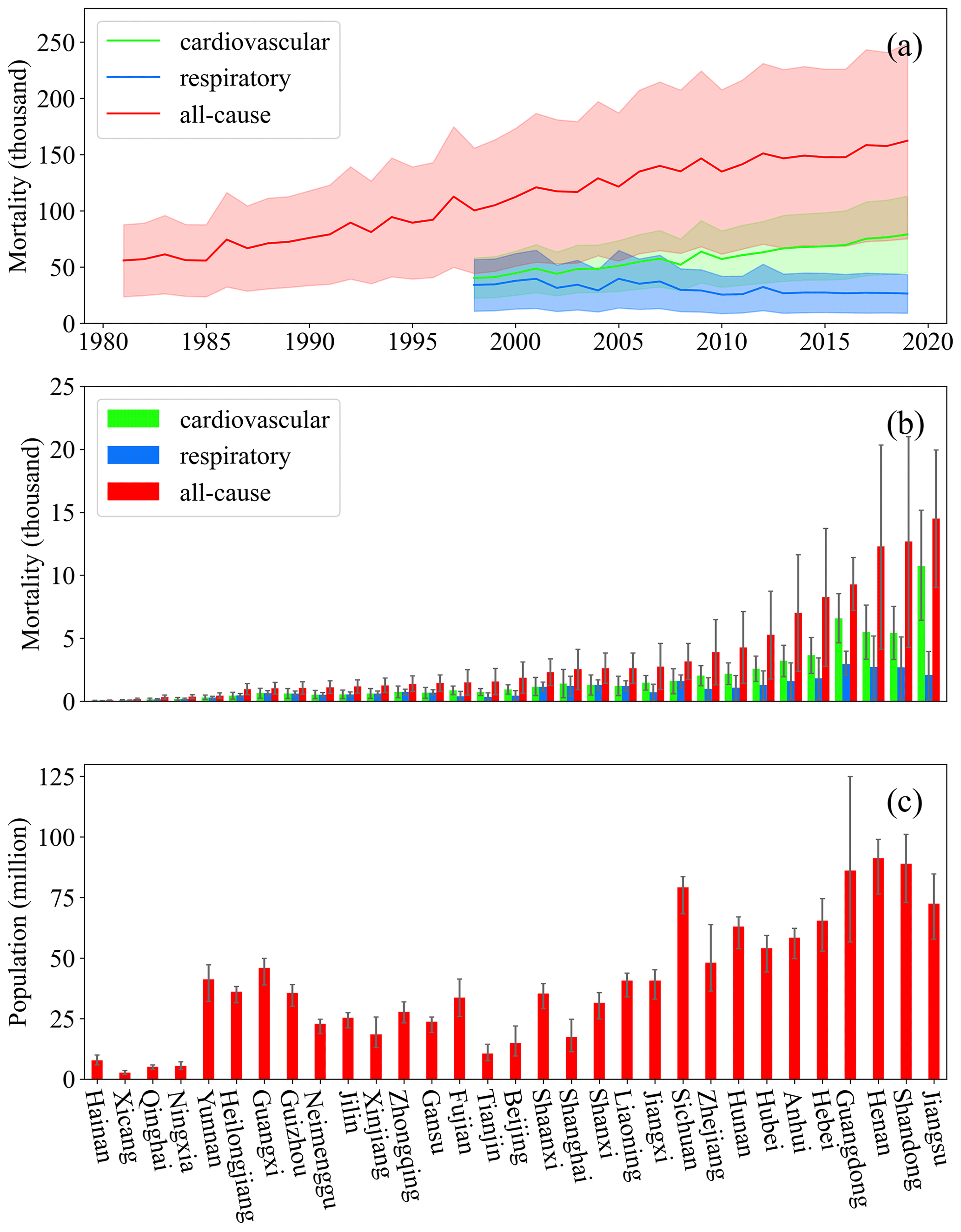
Figure 10 (a) Annual premature mortality (in thousands) for different diseases over the past few decades, (b) annual mean province-based mortality (in thousands) attributed to different health endpoints, and (c) annual mean province-based population (in millions). The mortality is calculated using the bias-corrected O₃.

3.6 Health impacts attributable to O₃ pollution

The estimated annual all-cause premature deaths induced by O₃ increased from 55 876 in 1981 to 162 370 in 2019 with an increasing trend of +2979 deaths per year. The annual premature deaths related to respiratory and cardiovascular diseases were 34 155 and 40 323 in 1998 and 26 471 and 79 021 in 2019, having a rate of change of −546 and +1773 deaths per year during 1998–2019, respectively (Fig. 10a). Among three types of health outcomes, only respiratory diseases experienced a decreasing trend in premature mortality, and the premature mortality is constantly below 40 000. The decreasing trend of the respiration-related mortality primarily results from the decreased annual baseline mortality rate over the past few decades (Fig. S14). As the total respiratory-related deaths decreased over the past few decades, respiratory O₃-related deaths are decreasing even under aggravated O₃ pollution. Based on GEOS-Chem-simulated O₃, the corresponding estimated change rate for all-cause disease is +3516 deaths per year from 50 384 in 1981 to 176 741 in 2019. Premature mortality induced by respiratory disease decreased from 37 822 in 1998 to 29 079 in 2019 with a change rate of −584 deaths per year, while cardiovascular disease increased from 44 516 in 1998 to 85 980 in 2019 with a change rate of +1977 deaths per year (Fig. S15). The result shows that using GEOS-Chem-simulated O₃ generally gives higher estimates of mortality than using the bias-corrected data. Figure 10b shows the provincial annual average premature mortality of different health endpoints. The five provinces with the highest all-cause mortality are Jiangsu (14 510; 95 % CI: 9022–19 935), Shandong (12 684; 95 % CI: 4258–20 990), Henan (12 290; 95 % CI: 4125–20 343), Guangdong (9268; 95 % CI: 7224–11 416), and Hebei (8276; 95 % CI: 2776–13 706), which are generally consistent with previous studies for China (Zhang et al., 2021, 2022a). Similar distribution can be found for respiratory and cardiovascular diseases but with a different ranking order. Generally, the provinces in densely populated areas (Fig. 10c) with higher O₃ concentrations, such as BTHs, YRD, and PRD, have higher health burdens. In contrast, northeastern and southern China (excluding Guangdong) suffer the least life losses induced by O₃ exposure (Fig. S16).

When compared with estimates from previous studies, our estimates are generally quite consistent with those given by Maji and Namdeo (2021), who reported that the short-term all-cause, cardiovascular, and respiratory premature mortalities attributed to ambient O₃ exposure were 156 000, 73 500, and 28 600 in 2019, respectively. Based on O₃ observations in 334 Chinese cities, Zhang et al. (2021) suggested that the national all-cause, respiratory, and cardiovascular mortalities attributable to O₃ were 270 000 to 390 000, 49 000 to 63 000, and 150 000 to 220 000 across 2015–2018, respectively, which are much higher than most existing results. Since the methodological approaches are largely similar and since we use the log-linear exposure–response function, we attribute the very high estimated mortalities mainly to the concentration–response threshold X₀ assumed to be 0 in their study. A lower X₀ means that O₃ can cause more adverse impacts on human health even at low concentrations, thus leading to higher mortalities.

4 Conclusions and discussion

In this study, to have a more accurate characterization of O₃ spatiotemporal distribution and trends as well as its impacts on agriculture and human health, we used a hybrid approach to generate bias-corrected O₃ data across China from 1981 to 2019. The hybrid approach helps improve O₃ predictions by taking advantage of a chemical transport model and a ML algorithm as well as increasing availability of high-resolution environmental and meteorological data. In the model training process, we found that utilizing a higher-resolution meteorological dataset, albeit one that is not the same as the default CTM input meteorology, has high potential to enhance the performance of the hybrid model in reproducing observed O₃ concentrations. The validation shows that the bias-corrected O₃ can achieve a higher prediction accuracy than the GEOS-Chem-simulated O₃ alone when compared with historical in situ measurements. Before being corrected, the GEOS-Chem-simulated O₃ concentrations tend to be overestimated, which leads to higher crop yield losses and larger O₃-induced mortalities. Noticeable differences in crop RYLs and mortality estimates highlight the advantages of using high-resolution O₃ data to improve our understanding of long-term O₃ impacts.

When examining the regional and national O₃ trends, we found that MDA8 O₃ concentrations have a perceptible increasing trend before the 2000s but fluctuate within a certain range with large interannual variabilities in more recent years. The large discrepancies in previous studies indicate that the regional and national O₃ trends in China still suffer great uncertainties, particularly when different approaches are used to produce the O₃ estimates. However, these studies using source-varied O₃ fields consistently show the great interannual variabilities of O₃ concentrations. Some insights can be obtained from existing findings, which need to be carefully considered when examining O₃ trends and comparing them with existing results. First, given the large site differences, the calculation of observational O₃ trends is very sensitive to the subsets of data from networks. Thus, great uncertainty could still exist even when using O₃ observations from the same source depending on the chosen subsets of data. Second, different formats of O₃ fields (e.g., site-based and gridded) could lead to large uncertainties in the O₃ trend estimates. A higher resolution of gridded O₃ estimates from CTMs and ML may reduce the differences between O₃ observational results. Third, the calculated O₃ trends are very sensitive to the chosen study period due to large interannual variability and seasonal differences. The changing meteorological conditions are the major factor causing the large interannual O₃ variations, and reductions in the emissions of NO_x, SO₂, and PM also have complex effects on ground-level O₃ concentrations (T. Wang et al., 2022). Liu and Wang (2020a) suggested that the meteorological impacts on O₃ trends vary from region to region and year by year and that it could be comparable with or even larger than the impacts of changes in anthropogenic emissions.

Our estimated RYLs for maize and rice in China are generally consistent with existing studies, while the RYLs for soybean and wheat are lower than their estimates, mainly due to the differences in the metrics used, O₃ fields, and crop sensitivity to ambient O₃ concentrations. It suggests that plating O₃-resistant cultivars could be an effective approach to increase total crop production to meet increasing food demands. Although other metrics (e.g., M7, M12, and W126) have also been used in some studies (Van Dingenen et al., 2009; Avnery et al., 2013; Y. Wang et al., 2022), exposure–yield relationships are not available for all four major crops specific to China. The estimated RYLs for crops could be largely biased using metrics with exposure–yield relationships developed for the US or Europe (Fig. S17), as they are inadequate to represent Asian crop genotypes and environmental conditions. Therefore, the region-specific exposure–yield relationships are highly recommended to be used in future studies estimating O₃-induced crop reduction, especially for regional studies.

In recent years, although existing studies have made efforts to quantify the O₃-related health impacts in China, only a few studies have focused on nationwide acute O₃ health burden assessment, particularly for assessment over multiple decades (Maji and Namdeo, 2021; Sahu et al., 2021; Zhang et al., 2021., 2022a). There are some remaining issues to be addressed regarding O₃ health impacts. For instance, the existence of a “safe” threshold of O₃ levels is still debated. A recent study reported that no consistent evidence was found for a threshold in the O₃ mortality concentration–response relationship in seven cities of Jiangsu Province, China, during 2013–2014 (Chen et al., 2017; Maji and Namdeo, 2021). Given the importance of the threshold assumption in assessing health effects of air pollution, more studies are needed to determine a most likely threshold for O₃ mortality association in the future. Moreover, the multiple temporal O₃ metrics (e.g., 1 h maximum and daytime average O₃ concentrations) have also proved to play an important role in the variability of estimated health effects, even though standard ratios are used to convert among multiple metrics (Anderson and Bell, 2010). In addition to the uncertainties from varying methodologies, interpretation of the O₃ epidemiological impact is also constrained by the variability in geographical, seasonal, and demographic characteristics (P. Yin et al., 2017). Liu et al. (2013) suggested that associations between O₃ and mortality appeared to be more evident during the cool season than in the warm season and stronger in the oldest age group and among those with less education. The effect modification by population susceptibility and the confounding effects of concomitant exposures (e.g., temperature, particulate matter) should be further considered in future work.

A major limitation of our study lies in the uncertain predictions in regions where monitoring data are scarce (e.g., the western half of China). The monitoring sites are sparsely distributed in those areas, which may fail to capture the accurate association between O₃ concentrations and various predictors there, especially considering that the ML algorithm has likely over-emphasized such relationships in the data-intensive eastern regions. Second, the land use data were prescribed in 2013 due to the limited availability of data, and this may neglect some major land use changes in China over the past few decades. Although the land use data were found by the ML algorithm to contribute little to the overall model, more detailed land use data are expected to further increase model accuracy. In addition, although concentration-based metrics are easy to calculate and ensured to be scientifically sound in some experiments (Fuhrer et al., 1997; Mills et al., 2007), they do not consider the active responses of plant ecophysiology to ambient climatic and environmental changes and are thus likely inadequate for examining yield losses in a future climate and atmospheric environment (Tai et al., 2021). Therefore, flux-based metrics are recommended in future studies to better understand the long-term evolution of crop losses over China (Feng et al., 2012; Zhang et al., 2017; Tai et al., 2021; Pleijel et al., 2022), wherein more crop- and region-specific experiments and trials are needed to acquire appropriate metrics and exposure–yield response functions and calibrate the process-based crop model.

Despite these limitations, our study represents important progress in evaluating the long-term, multidecadal health burdens and agricultural losses resulting from O₃ pollution in China. Across the four major regions, BTHs experience the highest RYLs for major crops due to elevated O₃. On the other hand, the YRD and PRD regions have greater human health losses primarily due to their large population size. The results can provide important references for governments and agencies when making related national or regional policies to meet imperative environmental, health, and food security demands. To effectively address the impacts of O₃, collaborative efforts can be made in multifaceted aspects: (1) implement stricter regulations and specific emission control measures for major ozone precursors from industrial, vehicular, and agricultural sources that account for region-specific chemical, meteorological, and terrestrial conditions; (2) encourage the adoption of more sustainable and adaptive agricultural practices that minimize O₃ exposure and its damage on crops (e.g., cultivating O₃-resistant crop varieties); (3) improve short-range O₃ forecast capabilities of regional models, especially with the enhancement of artificial intelligence technology, which may enable better early-warning systems to prepare the public and farmers for O₃ episodes; and (4) raise public awareness via promotional campaigns and educational programs to inform individuals, communities, and farmers about the risks associated with O₃. It is important for policymakers to consider these suggestions and act to effectively mitigate the negative impacts of O₃.