Evaluation of vertical transport in ERA5 and ERA-Interim reanalysis using high-altitude aircraft measurements in the Asian summer monsoon 2017

During the Asian monsoon season, greenhouse gases and pollution emitted near the ground are rapidly uplifted by convection up to an altitude of ∼ 13 km, with slower ascent and mixing with the stratospheric background above. Here, we address the robustness of the representation of these transport processes in different reanalysis data sets using ERA5, ERA-Interim and ERA5 $\mathrm{1}{}^{\circ }\times \mathrm{1}{}^{\circ }$. This transport assessment includes the mean age of air from global three-dimensional simulations by the Lagrangian transport model CLaMS (Chemical Lagrangian Model of the Stratosphere), as well as different trajectory-based transport times and associated ascent rates compared with observation-based age of air and ascent rates of long-lived trace gases from airborne measurements during the Asian summer monsoon 2017 in Nepal.

Our findings confirm that the ERA5 reanalysis yields a better representation of convection than ERA-Interim, resulting in different transport times and air mass origins at the Earth's surface. In the Asian monsoon region above 430 K, the mean age of air driven by ERA-Interim is too young, whereas the mean age of air from ERA5 $\mathrm{1}{}^{\circ }\times \mathrm{1}{}^{\circ }$ is too old but somewhat closer to the observations. The mean effective ascent rates derived from ERA5 and ERA5 $\mathrm{1}{}^{\circ }\times \mathrm{1}{}^{\circ }$ back trajectories are in good agreement with the observation-based mean ascent rates, unlike ERA-Interim, which is much faster above 430 K. Although a reliable CO₂ reconstruction is a challenge for model simulations, we show that, up to 410 K, the CO₂ reconstruction using ERA5 agrees best with high-resolution in situ aircraft CO₂ measurements, indicating a better representation of Asian monsoon transport in the newest ECMWF reanalysis product, ERA5.

1 Introduction

The global amount of greenhouse gases (GHGs) in the atmosphere has increased because of worldwide anthropogenic emissions. In particular, the rapid increase in anthropogenic CO₂ emissions in southern Asia contributes strongly to the acceleration of the CO₂ growth rate; e.g. the anthropogenic CO₂ emission rate from India was the fourth highest worldwide in 2017 (behind China, the USA and the European Union) (Friedlingstein et al., 2019, 2022). In addition to GHGs, pollution, water vapour, aerosol particles and their precursors, as well as some ozone-destroying substances, also have high emission rates in Asia and can be transported very fast into the lower stratosphere during the Asian summer monsoon season (e.g. Brunamonti et al., 2018; Hanumanthu et al., 2020; Adcock et al., 2021; Appel et al., 2022; Vogel et al., 2023). Subsequently these trace gases and aerosol particles can be distributed into the global northern lower stratosphere over a period of several weeks (e.g. Ploeger et al., 2013; Müller et al., 2016; Vogel et al., 2016; Yu et al., 2017; Rolf et al., 2018; Lauther et al., 2022). To better understand the impact of anthropogenic emissions in Asia on the atmosphere, it is important to evaluate the transport of air in the Asian summer monsoon region into the lower stratosphere, represented in meteorological reanalyses in combination with unique high-resolution aircraft measurements obtained over the northern Indian subcontinent during the StratoClim aircraft campaign in summer 2017 (Stroh and StratoClim-Team, 2023).

From about June to September, the Asian summer monsoon constitutes a seasonally persistent, zonally restricted circulation pattern transporting climate-relevant emissions rapidly from surface sources to higher altitudes, i.e. to the lower stratosphere (e.g. Mason and Anderson, 1963; Randel and Park, 2006; Park et al., 2007; Pan et al., 2016; Vogel et al., 2015; Ploeger et al., 2017; Vogel et al., 2023). The Asian summer monsoon is associated with deep convection over the Indian subcontinent and an anticyclonic flow in the upper troposphere and lower stratosphere (UTLS) over the Asian monsoon region, spanning from northeast Africa to the Pacific (e.g. Park et al., 2007). Air parcels are uplifted quickly by convection followed by slow diabatic uplift in the UTLS superimposed on the anticyclonic flow (e.g. Brunamonti et al., 2018; Vogel et al., 2019; Legras and Bucci, 2020; von Hobe et al., 2021), while in other regions within the tropical transition layer the heating rates are, in general, smaller during boreal summer (Vogel et al., 2019). The higher the air parcels are located above the level of maximum convective outflow (∼ 360 K, ∼ 13 km), the larger the contribution of air masses is from outside the Asian monsoon anticyclone (i.e. from the stratospheric background) to the upward spiralling flow (Vogel et al., 2019, 2023).

In state-of-the-art chemistry transport models, the transport of air parcels differs because different methods (Eulerian, Lagrangian), different vertical velocities (kinematic, diabatic) and different meteorological reanalyses are used to drive the models (e.g. Stenke et al., 2009; Bergman et al., 2013; Brinkop and Jöckel, 2019; Tao et al., 2019; Ploeger et al., 2019; Bucci et al., 2020; Legras and Bucci, 2020; Tegtmeier et al., 2020; Clemens et al., 2023). Further, the implementation of convection and irreversible mixing differs from model to model (e.g. Brinkop and Jöckel, 2019; Konopka et al., 2019; Wohltmann et al., 2019; Hoffmann et al., 2023). The aim of this study is to infer differences of vertical transport in the Asian monsoon region using three data sets: two reanalyses provided by the European Centre for Medium-Range Weather Forecasts (ECMWF), namely, ERA-Interim and its successor ERA5, as well as its down-scaled version ERA5 $\mathrm{1}{}^{\circ }\times \mathrm{1}{}^{\circ }$, a computing-time-saving alternative to the full-resolution ERA5 data.

In general, differences between ERA-Interim and ERA5 are attributed to the better spatial and temporal resolution of the ERA5 reanalysis, which allows for a better representation of convective updrafts, gravity waves and tropical cyclones (e.g. Hoffmann et al., 2019; Li et al., 2020; Legras and Bucci, 2020; Malakar et al., 2020). Consequently, ERA5 provides a more accurate representation of the lapse rate tropopause height than ERA-Interim (e.g. Hoffmann et al., 2022; Tegtmeier and Krüger, 2022).

In the Asian monsoon anticyclone, slow diabatic uplift in the range of 1–1.5 K d⁻¹ occurs above the level of maximum convective outflow using Lagrangian transport simulations driven by ERA-Interim (Vogel et al., 2019). However, it was found consistently in several previous studies that, in general, the vertical velocities in ERA-Interim are 30 %–50 % too fast in the tropics (Dee et al., 2011; Ploeger et al., 2012; Schoeberl et al., 2012). Tegtmeier and Krüger (2022) summarise that diabatic vertical ascent appears to be faster in ERA-Interim, which produces a residence time (between 370 and 400 K) of ∼ 2 months in the tropical tropopause layer in contrast to residence times of ∼ 3 months or longer based on other reanalyses (e.g MERRA, MERRA-2 or CFSR; however, ERA5 was not included here). This bias seems to be corrected in ERA5 manifesting weaker diabatic heating rates in the tropics, resulting in a greater age of air (i.e. larger mean stratospheric transit times) and thus a significantly slower Brewer–Dobson circulation in ERA5 compared to ERA-Interim (Ploeger et al., 2021). Different residence times in the UTLS would change the chemical composition at these altitudes, and even small changes of radiatively active trace gases such as O₃, H₂O or aerosol particles could have important local radiative impacts (e.g. Riese et al., 2012; Vernier et al., 2015; Fadnavis et al., 2019; Bian et al., 2020).

For the StratoClim aircraft campaign during the Asian summer monsoon of 2017 (denoted monsoon 2017), in general, a higher consistency with observations and a better reproducibility of pollution features could be found in diabatic trajectory calculations back to cloud top altitudes using ERA5 compared to ERA-Interim (Bucci et al., 2020). ERA5 improves, in general, the transport in the Asian monsoon 2017; however, upward transport in the region of the Tibetan Plateau should be considered with caution (Legras and Bucci, 2020). Considering the transport of air masses contributing to the Asian Tropopause Aerosol Layer (ATAL) measured in the region of the Asian monsoon anticyclone during August 2016, ERA5 shows, in general, faster transport of air from the ground to ATAL altitudes (up to ≈ 410 K) due to a better representation of convection. In addition, more continental source regions contributing to the ATAL are found in ERA5, whereas in ERA-Interim, more marine sources are attributed to air at ATAL altitudes (Clemens et al., 2023).

Using ERA-Interim compared to ERA5 reanalysis yields different vertical velocities or ascent rates in the region of the Asian monsoon anticyclone, which has consequences for global transport simulations. To assess such global simulations, it is essential to understand the strengths and weaknesses of the newest ECMWF product, ERA5, particularly in the Asian monsoon region. In this work, differences in the transport of air in the regions of the Asian summer monsoon 2017 will be inferred using the Chemical Lagrangian Model of the Stratosphere (CLaMS), driven by the three data sets (ERA-Interim, ERA5 and ERA5 $\mathrm{1}{}^{\circ }\times \mathrm{1}{}^{\circ }$). Model results will be assessed using unique airborne measurements up to ∼ 20 km during the Asian summer monsoon of 2017 conducted during the StratoClim aircraft campaign in Nepal (Stroh and StratoClim-Team, 2023). Trajectory-based transport times, origin of air at the Earth's surface, mean effective ascent rates, transport time distribution and the mean age of air from three-dimensional CLaMS simulations are compared using the three data sets (ERA-Interim, ERA5 and ERA5 $\mathrm{1}{}^{\circ }\times \mathrm{1}{}^{\circ }$). In addition, the simulated mean age of air is compared to observation-based mean age of air inferred from long-lived trace gases such as C₂F₆, HFC-125, SF₆ and N₂O. In addition, C₂F₆ and HFC-125 are used to compare observation-based mean ascent rates with those from different reanalyses.

Further, a unique set of CO₂ aircraft measurements featuring high temporal and vertical resolutions up to ∼ 20 km were obtained during the StratoClim aircraft campaign of 2017 (Stroh and StratoClim-Team, 2023). Measured CO₂ profiles were successfully reconstructed using ground-based measurements of CO₂, mainly from Nainital (northern India), by Lagrangian model simulations using ERA5 reanalysis, leading to an improved understanding of the vertical structure of CO₂ in the monsoon region (Vogel et al., 2023). Here, we use the same CO₂ reconstruction method as that used in Vogel et al. (2023), but we focus on the differences between the three data sets (ERA-Interim, ERA5 and ERA5 $\mathrm{1}{}^{\circ }\times \mathrm{1}{}^{\circ }$). In general, our results show that using ERA5 reanalysis yields a better agreement with aircraft measurements conducted over the Indian subcontinent in summer 2017 compared to ERA-Interim.

2 Measurements during the Asian summer monsoon of 2017

In the frame of the StratoClim project funded by the European Commission, a measurement campaign using the Russian Geophysica, a high-altitude research aircraft, was conducted in Kathmandu (Nepal) in summer 2017 (see Fig. 1) to measure a variety of trace gases and aerosol characteristics for the first time in the Asian monsoon anticyclone up to 20 km altitude (corresponding to ∼ 55 hPa or ∼ 475 K potential temperature) (Stroh and StratoClim-Team, 2023). The StratoClim measurements constitute a unique data set to characterise major processes which dominate particle and trace gas transport from the northern Indian subcontinent, one of the most polluted regions of the world, into the lower stratosphere.

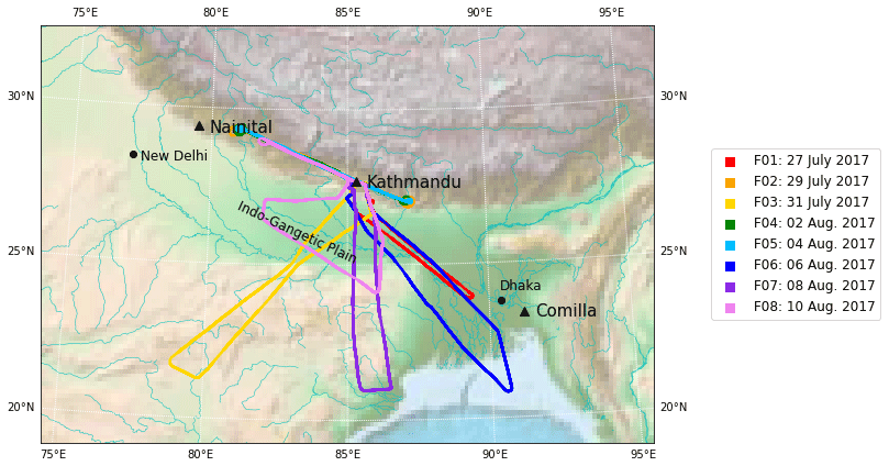
Figure 1 Regional map of the aircraft measurements over the Indian subcontinent. The flight paths of the eight local scientific flights (F01–F08) by the high-altitude research aircraft Geophysica are shown. The scientific flights were carried out every second day from Kathmandu (Nepal) between 27 July and 10 August 2017. In addition, the locations of the measurement sites for greenhouse gases in Nainital (NTL, India) and Comilla (CLA, Bangladesh) used for CO₂ reconstruction are indicated (figure adapted from Vogel et al. (2023)).

CO₂ and N₂O were detected using the multi-tracer in situ instrument HAGAR (Werner et al., 2010; Homan et al., 2010), operated by the University of Wuppertal. Apart from CO₂ and N₂O, it also provides simultaneous in situ measurements of CH₄, CFC-12, CFC-11, H-1211, SF₆ and H₂. Except for CO₂, which is measured at a high time resolution (3 to 5 s) by non-dispersive infrared absorption (NDIR), all the other species were measured by gas chromatography with electron capture detection (GC/ECD) every 90 s. The instrument is calibrated every 7.5 min during flight with either of the two standard gases, which are inter-calibrated in the laboratory with standards provided by NOAA GML. For StratoClim, the accuracy of CO₂ was estimated to be about 0.2 ppm and about 2 ppb for N₂O (more details can be found in Vogel et al., 2023).

The long-lived trace gases C₂F₆, HFC-125 and SF₆ were collected with the whole-air sampler of Utrecht University operated on board the Geophysica research aircraft (e.g. Laube et al., 2010a). Ambient air was compressed into evacuated stainless-steel canisters (2 L) using a metal bellows pump that has been previously been shown not to impact trace gas mixing ratios (e.g. Kaiser et al., 2006). The samples were transported to the University of East Anglia (UEA) for analysis on a high-sensitivity gas chromatograph–trisector mass spectrometer system (Laube et al., 2010b). More details on the whole-air sampler measurements during StratoClim and the used analytical technique can be found in Adcock et al. (2021).

3 Lagrangian transport simulations

3.1 CLaMS trajectory calculations

Back trajectory calculations were performed using the trajectory module of the Chemical Lagrangian Model of the Stratosphere (CLaMS) (McKenna et al., 2002b, a; Pommrich et al., 2014, and references therein), which was developed with the aim of studying transport and chemical processes in the atmosphere in the presence of strong tracer gradients. Here, CLaMS diabatic backward trajectories were started along the complete flight tracks (every 1 s) of all eight StratoClim Geophysica research flights (F01-F08) conducted over the northeastern part of the Indian subcontinent. Depending on the length of the flights, between 9000 and 16 000 back trajectories are calculated per research flight, in total ∼ 110 000 back trajectories.

For comparison, the back trajectory calculations are driven by three data sets, including two different reanalyses and one of them in different resolution, provided by the European Centre for Medium-Range Weather Forecasts (ECMWF): ERA-Interim, ERA5 and ERA5 $\mathrm{1}{}^{\circ }\times \mathrm{1}{}^{\circ }$. The new ERA5 reanalysis (Hersbach et al., 2020) is a high-resolution atmospheric data set with 137 vertical levels up to 0.01 hPa, a horizontal resolution of ∼ 31 km (T_L 639) and an hourly time resolution. We retrieved the data on a 0.3${}^{\circ }\times$0.3^∘ horizontal grid. The ECMWF's prior reanalysis ERA-Interim (Dee et al., 2011) has 60 vertical levels up to 0.01 hPa, a horizontal resolution of ∼ 79 km (T_L 255) (corresponding to 1${}^{\circ }\times$1^∘ horizontal grid) and a 6-hourly time resolution.

Further, we use a version of ERA5 with a lower resolution, referred to as ERA5 $\mathrm{1}{}^{\circ }\times \mathrm{1}{}^{\circ }$ (similar to Ploeger et al., 2021; Konopka et al., 2022; Clemens et al., 2023). ERA5 $\mathrm{1}{}^{\circ }\times \mathrm{1}{}^{\circ }$ data are directly provided by the ECMWF on a $\mathrm{1}{}^{\circ }\times \mathrm{1}{}^{\circ }$ horizontal grid after down-scaling the original data by truncation of the spherical harmonics representation to a 1${}^{\circ }\times \mathrm{1}{}^{\circ }$ horizontal grid (corresponding to T_L 255). In addition, the time resolution is down-sampled to every 6 h for better comparability with ERA-Interim. However, the vertical resolution is not changed and is the same as in the original ERA5 reanalysis. ERA5 $\mathrm{1}{}^{\circ }\times \mathrm{1}{}^{\circ }$ data are a computing-time-saving alternative to the full-resolution ERA5 data and are particularly suited for three-dimensional, global, multi-annual CLaMS simulations.

In the CLaMS model, potential temperature is used as the vertical coordinate when the pressure is less than about 300 hPa, (i.e. in the upper troposphere and in the stratosphere); when the pressure is greater than about 300 hPa (more accurately, for pressure p exceeding a reference level of $p/p_{\mathrm{surface}}=\mathrm{0.3}$), a pressure-based orography-following hybrid coordinate (in units of K) is used (Pommrich et al., 2014). In potential temperature levels above about 300 hPa, the vertical velocity (i.e. dΘ $/$ dt) is determined solely by the total heating rate (Pommrich et al., 2014; Ploeger et al., 2021). Total diabatic heating rates including clear-sky radiative heating, cloud radiation, latent heat release, and turbulent and diffusive heat transport for the upper troposphere and stratosphere are deduced from ECMWF reanalyses. However, in the first layers below the reference level, the vertical coordinate is also still close to diabatic as the transition from potential temperature to an orography-following vertical coordinate occurs rather slowly (e.g. Pommrich et al., 2014). Therefore, the vertical velocity includes information on convective transport as resolved in the reanalysis vertical wind and total diabatic heating rate (see Pommrich et al., 2014).

Trajectories are considered to end in the model boundary layer, referred to as model BL, when they are located for the first time below about 2–3 km above the surface considering orography (i.e. the vertical hybrid pressure–potential–temperature coordinate (ζ) fulfils ζ≤ 120 K) (for details, see e.g. Vogel et al., 2015, 2019).

The upward transport and convection in CLaMS (in both trajectory calculations and three-dimensional simulations) depend on the employed reanalysis data (ERA-Interim, ERA5, ERA5 $\mathrm{1}{}^{\circ }\times \mathrm{1}{}^{\circ }$), which differ strongly in the representation of convection (e.g. Hoffmann et al., 2019; Li et al., 2020; Clemens et al., 2023). The differences between ERA5 and ERA-Interim are attributed to, among other issues, the better spatial and temporal resolutions of the ERA5 reanalysis, which allow for a better representation of convective updrafts. Therefore, in ERA-Interim, convection over Asia is underestimated compared to ERA5. In our study, no additional parameterisation for convection is used for the CLaMS simulations; only the convection already included in the reanalysis is considered.

3.2 Method for CO₂ reconstruction

Vogel et al. (2023) demonstrated that high-resolution CO₂ profiles measured in situ during the StratoClim campaign in summer 2017 reflect the seasonal variability of CO₂ at ground level. In addition, CO₂ is chemically inert in the troposphere and stratosphere and can be used as an age tracer considering time periods of several months (e.g. Boering et al., 1996; Andrews et al., 2001; Ray et al., 2022). Therefore a reasonable reconstruction of vertical CO₂ was conducted successfully using CLaMS back trajectories driven by ERA5 reanalysis using ground-based CO₂ measurements (Vogel et al., 2023). Following the approach by Vogel et al. (2023), here, we apply the same method for CO₂ reconstruction; however, the differences between ERA5 compared to ERA-Interim and ERA5 $\mathrm{1}{}^{\circ }\times \mathrm{1}{}^{\circ }$ will be analysed to infer possible differences in the transport of air masses between the three data sets.

The method for CO₂ reconstruction used in Vogel et al. (2023) is briefly summarised hereafter. CO₂ mixing ratios from ground-based observations on the Indian subcontinent (Fig. 2) measured during the time when the CLaMS back trajectories reach the model BL are used for CO₂ reconstruction. For that purpose, different CO₂ ground-based observations (all shown in Fig. 3) available on different timescales (monthly, weekly or daily) were interpolated in time on a common daily grid to get a CO₂ mixing ratio for every day from each used measurement site for the CO₂ reconstruction. These calculated CO₂ mixing ratios define CO₂ in the model boundary layer and are transported passively along the trajectory to the location and time of the Geophysica flight path; i.e. CO₂ is treated as chemically inert over the time of the back trajectory calculation.

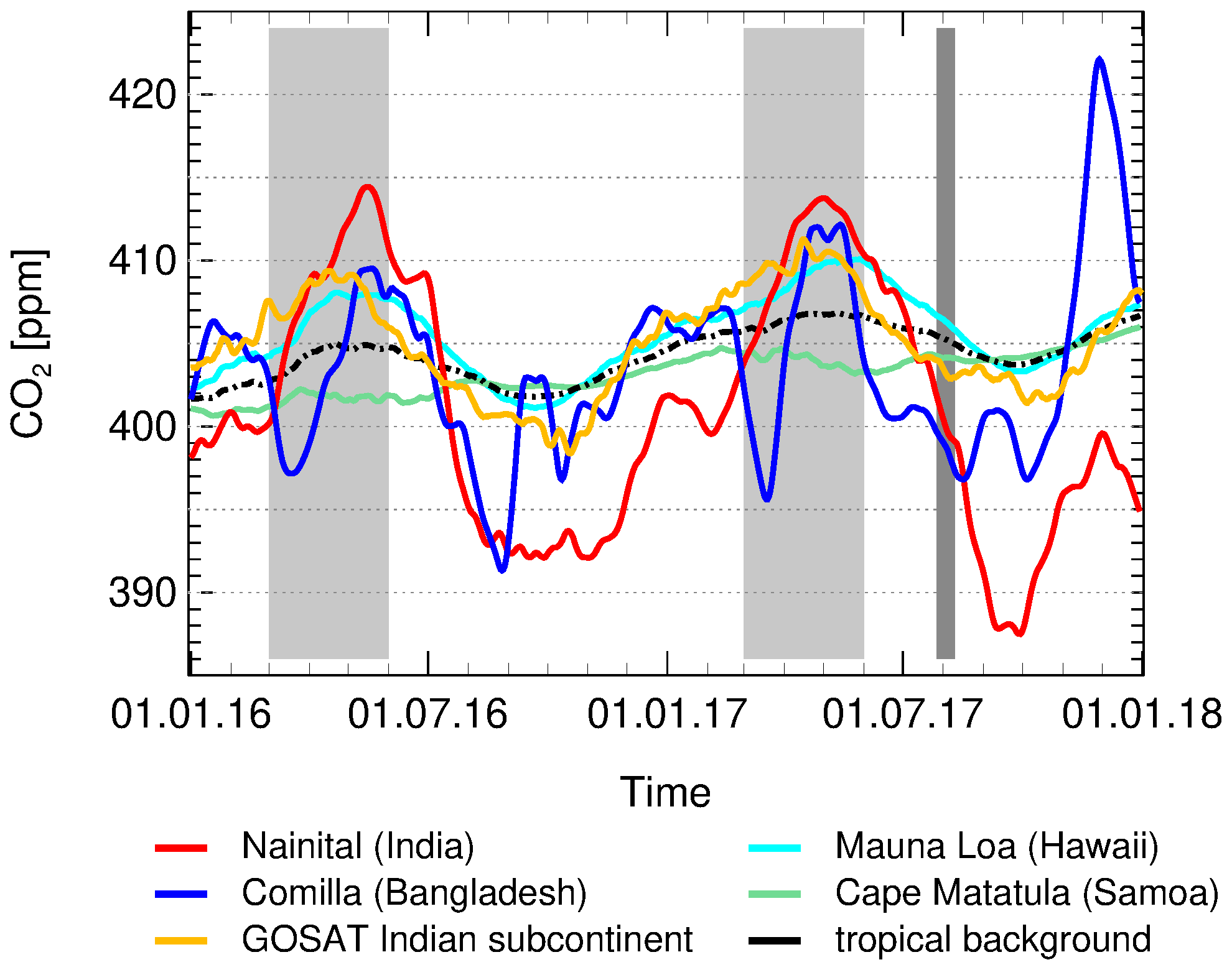
Figure 2 Temporal variability of ground-based CO₂. The variability of ground-based CO₂ is shown at Nainital and Comilla (for geographical positions, see Fig. 1). In addition, the seasonal variability of CO₂ over the northern Indian subcontinent (mean value between 20–30^∘ N and 75–95^∘ E) at the lowest model level (975 hPa) of the GOSAT-L4B product for comparison to ground-based CO₂ measurements is shown. Further, ground-based CO₂ measured in Mouna Loa (Hawaii) and in Cape Matatula (Samoa), as well as their averages (dash-dotted black line) as reference for the tropical background, are given. The pre-monsoon period (March–May) when a seasonal CO₂ maximum is expected is highlighted (light grey), along with the period of the StratoClim aircraft campaign during monsoon 2017 (dark grey).

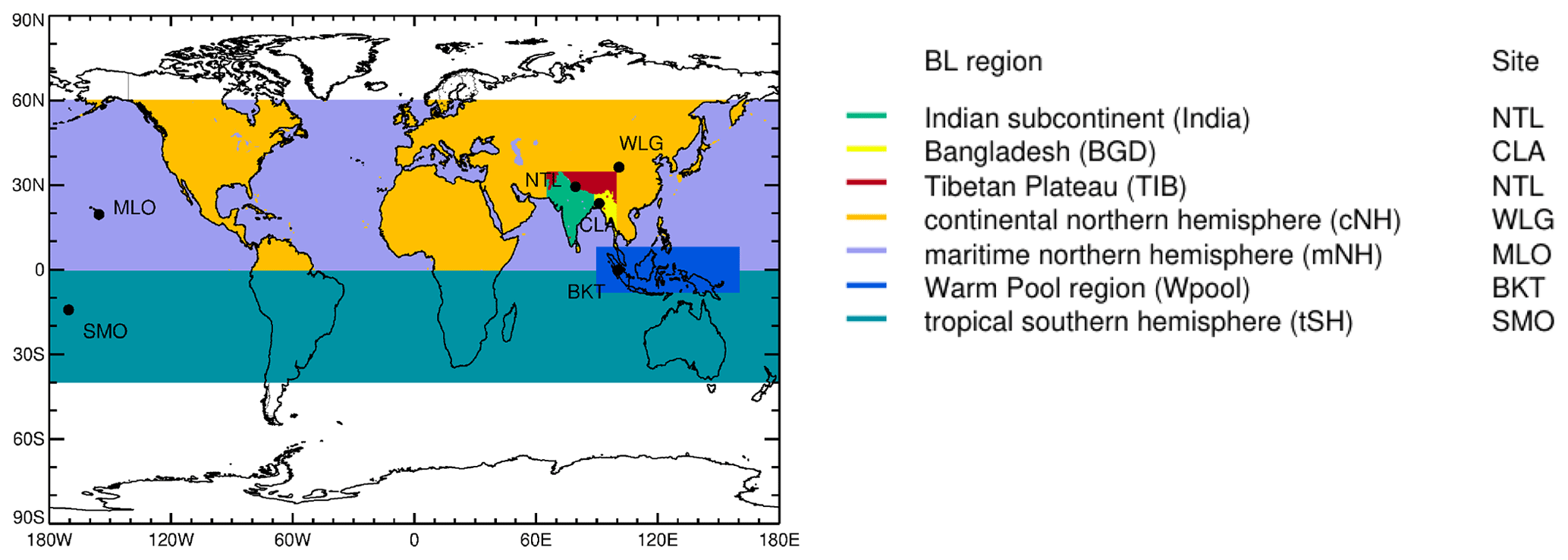
Figure 3 Regional mask for CO₂ reconstruction using CO₂ ground-based measurements at different sites in Asia and the Pacific. In each model boundary layer (BL) region (marked by different colours), CO₂ is prescribed from one specific measurement site: the tropical Southern Hemisphere (tSH) by Samoa (SMO), the Indian subcontinent (India) by Nainital (NTL), Bangladesh (BGD) by Comilla (CLA), the Tibetan Plateau (TIB) by Nainital (NTL), the marine Northern Hemisphere (mNH) by Mauna Loa (MLO), the continental Northern Hemisphere (cNH) by Mount Waliguan (WLG) and the Warm Pool region (Wpool) by Bukit Kototabang (BKT) (figure adapted from Vogel et al. (2023)).

As a second step, a regional mask was developed where CO₂ is prescribed in the model BL depending on different geographical regions (see Fig. 3). In each of these geographical regions, referred to as the BL region, CO₂ is prescribed using one specific measurement site; e.g. trajectories ending in the BL region marked in green and dark red (roughly the Indian subcontinent and Tibetan Plateau) are prescribed using ground-based measurements from Nainital, and the BL region marked in yellow (roughly Bangladesh) is prescribed using ground-based measurements from Comilla. Unfortunately the coverage of ground-based measurements of CO₂ over the Indian subcontinent in 2016 to 2017 is sparse; therefore, only data from Nainital and Comilla are available. Additional CO₂ ground-based time series from other geographical regions influencing the Geophysica measurements provided by measurement sites for greenhouse gases in Mount Waliguan (WLG, China), Bukit Kototabang (BKT, Indonesia), Mauna Loa (MLO, Hawaii) and Samoa (SMO, Cape Matatula) are used for CO₂ reconstruction (more details about the used ground-based observations can be found in Vogel et al., 2023).

Ground-based CO₂ values (provided by the World Data Centre for Greenhouse Gases (WDCGG), https://gaw.kishou.go.jp) measured in Mouna Loa (Hawaii) and in Cape Matatula (Samoa) (Thoning et al., 2021), as well as their average (dash-dotted black line), are also shown in Fig. 2 as a reference for the tropical background (e.g. Boering et al., 1996; Andrews et al., 1999). The comparison of the different seasonal cycles of the ground-based CO₂ measurements demonstrates that the seasonal CO₂ maximum over the Indian subcontinent during pre-monsoon is much larger than the CO₂ maximum of ground-based CO₂ of the tropical background.

The definitions of the different model boundary layer regions are adjusted according to the available measurement sites. Case studies with different regional masks defining the model boundary layer regions were performed, and the regional mask was developed according to the best agreement of reconstructed and measured vertical CO₂ profiles. Further, the local air mass transport influencing Nainital is taken into account, as explained in Vogel et al. (2023).

The seasonal variability of CO₂ over the northern Indian subcontinent (mean value between 20–30^∘ N and 75–95^∘ E) at the lowest model level, 975 hPa, of the GOSAT-L4B product (Matsunaga and Maksyutov, 2018) is shown in Fig. 2 for comparison to ground-based CO₂ measurements. The GOSAT-L4B product is a model simulation using CO₂ surface fluxes inferred from column-averaged satellite measurements (Maksyutov et al., 2013). The lowest model level of GOSAT-L4B is closest to the inferred CO₂ surface fluxes and is not strongly influenced by the tracer transport of the underlying transport model. GOSAT-L4B CO₂ over the northern Indian subcontinent has the same seasonality as ground-based CO₂ over Nainital; however, the minimum and maximum values differ strongly, highlighting the need for ground-based CO₂ measurements over the Indian subcontinent in addition to satellite-based estimation of CO₂ surface fluxes (a more detailed discussion can be found in Vogel et al., 2023).

3.3 Mean age of air from three-dimensional CLaMS simulations

Trajectory-based transport times are compared to the mean age of air from global three-dimensional CLaMS chemistry transport model simulations performed over a time period of several decades to consider, in addition, the transport time of aged air, which is not considered in our back trajectory calculations ending on 1 June 2016. Global three-dimensional CLaMS simulations are based on three-dimensional forward trajectories and a parameterisation of small-scale mixing depending on the shear in the large-scale flow (e.g. Pommrich et al., 2014). The model simulations are driven with either ERA5 $\mathrm{1}{}^{\circ }\times \mathrm{1}{}^{\circ }$ or ERA-Interim reanalysis winds and diabatic heating rates, as described in more detail by Ploeger et al. (2021). Similarly to that for the CLaMS trajectory calculations, convection resolved in the reanalysis vertical winds and total diabatic heating rates are used for the three-dimensional CLaMS simulation (see Sect. 3.1). Apart from small-scale mixing, the vertical transport in CLaMS trajectory calculations and in the three-dimensional CLaMS simulations is treated in the same way.

Ploeger et al. (2021) performed global three-dimensional CLaMS simulations to calculate the age spectrum of the air and the distribution of transit times through the stratosphere at each location in the stratosphere based on chemically inert pulse tracers. In our study, the globally calculated mean age of air by Ploeger et al. (2021) is interpolated along all Geophysica flights paths (F01–F08). Thus, a direct comparison to the trajectory-based transport time is possible. In Ploeger et al. (2021), 60 different tracer pulses are released at the tropical surface (30^∘ S–30^∘ N), more specifically by a mixing ratio boundary condition in the lowest model layer. The chosen pulse frequency of 2 months allows a 2-month resolution of the age spectrum along the transit time axis for 10 years of transit time (more details in Ploeger et al., 2021). The mean age of air is calculated in three different ways to enable an assessment of the uncertainties arising from the method. First, the mean age is calculated as the first moment (mean) of the age spectrum. Second, this age-spectrum-based mean age is corrected for its finite tail (truncated to 10 years) by applying an exponential correction fit. Third, the mean age is also calculated from a clock tracer with a linear increase in the entire lowest model layer. Due to the methodological differences, the age-spectrum-based mean age is expected to yield the youngest estimate, the spectrum-based mean age including the tail correction yields the oldest estimate, and the clock tracer mean age values lie in between. The range between these three different mean age estimates can be interpreted as an estimate for methodological uncertainties arising from the mean age calculation. Compared to the trajectory-based transport times, all three mean age estimates are expected to result in higher values as they include the effects of mixing and recirculation of old stratospheric air into the tropics, which is absent in the pure trajectory calculations ending on 1 June 2016.

4 Results

CLaMS diabatic backward trajectories driven by three data sets (ERA-Interim, ERA5 and ERA5 $\mathrm{1}{}^{\circ }\times \mathrm{1}{}^{\circ }$) were started along all Geophysica flight tracks (F01–F08) to infer a trajectory-based transport time from the location of the measurement back to the time when the back trajectory reached the model BL. The trajectories are calculated back to 1 June 2016 and are analysed within different time periods to identify the source regions at the model BL depending on the season (see Table 1). However, most back trajectories reach the model BL much later than 1 June 2017, which implies that air parcels probed during the Geophysica flights were released at the model BL much later than 1 June 2017; e.g. 64 % (63 %) of all air parcels are from the monsoon season of 2017 using ERA5 (ERA-Interim) reanalysis.

Table 1 Time periods and the trajectory-based age of air of the considered seasons on the Indian subcontinent. The analysis of CLaMS back trajectories is performed back until the start time of each season. For each season, air parcels that were released at the model boundary layer (BL) are analysed. The longest simulation time is back until 1 June 2016 (∼ 1 year). Air parcels that are located in the free atmosphere on 1 June 2016 are considered to be aged air.

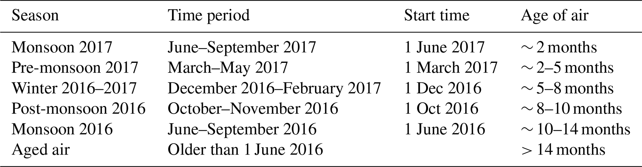
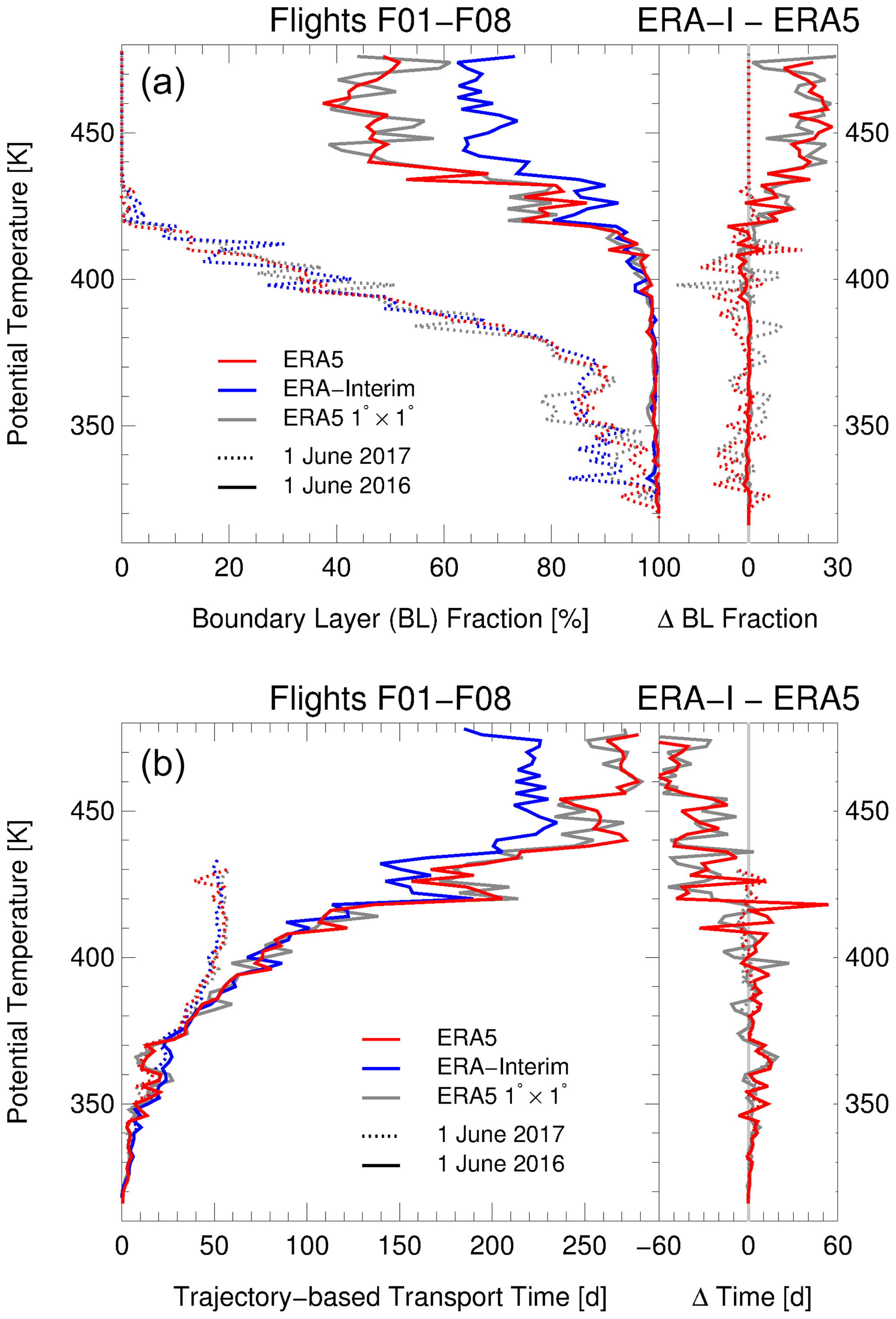
Figure 4 Mean fraction of air from the model BL (a) and the trajectory-based mean transport time (b) as calculated from all backward trajectories started along the Geophysica flight tracks averaged as the median in 2 K intervals and accumulated back to the start times of the monsoon of 2017 (1 June 2017, dotted lines) and the monsoon of 2016 (1 June 2016, solid lines). The trajectory calculations are driven by three data sets (ERA-Interim, ERA5 and ERA5 $\mathrm{1}{}^{\circ }\times \mathrm{1}{}^{\circ }$) indicated by different colours. The differences (Δ) between ERA-Interim and ERA5 (red) as well as between ERA-Interim and ERA5 $\mathrm{1}{}^{\circ }\times \mathrm{1}{}^{\circ }$ (grey) are shown in the right panels.

The higher the sampled air parcels are located, the longer their simulated trajectory-based transport times are, which is to be expected. However, there is also a strong variability of transport times between individual air parcels at the same level of potential temperature, indicating mixing of air masses of different transport times (or different ages) and of different origins.

4.1 Transport times and mean age of air

The mean fraction of air from the model BL and the trajectory-based mean transport time are calculated from all backward trajectories started along the Geophysica flight tracks depending on flight height. Figure 4 shows the trajectory-based mean transport time (averaged as the median in 2 K intervals) and the mean fraction of air from the model BL depending on potential temperature and accumulated back to the start times of the monsoon of 2017 and the monsoon of 2016 using the three data sets. To calculate the trajectory-based mean transport time, only the fraction of trajectories from the model BL is considered; thus, older air masses are neglected at first approximation.

All simulations show that considering a trajectory length back to the start time of the monsoon of 2017 yields a boundary layer fraction between 80 % and 100 % below 370 K; above 370 K, the boundary layer fraction decreases rapidly and reaches 0 % around 420 K (Fig. 4a). The transition at ∼ 370 K corresponds to the crossover level near 364 K found in the Asian summer monsoon of 2017 by Legras and Bucci (2020). The crossover level marks the separation between descending and ascending motion and thus confirms that convection as represented in the reanalysis data is included in CLaMS backward trajectories. Our results show that a trajectory length of about 2 months is too short for a comprehensive simulation of the chemical composition of the Asian monsoon anticyclone because only very young air masses are considered.

Using a trajectory length back to the start time of the monsoon of 2016 (≈ 10–14 months), a boundary layer fraction of almost 100 % is reached up to 410 K. Above, the boundary layer fraction is slowly decreased and depends strongly on the used ECMWF reanalysis (Fig. 4a) and implicates different mean transport times at these altitudes (Fig. 4b).

Below 410 K, convection in ERA5 yields faster transport times (up to ≈ 20 d) and higher model boundary layer (BL) fractions than in ERA-Interim. On the other hand, above 420 K, air masses have faster transport times by up to 2 months (≈ 60 d) from the model BL to the UTLS in ERA-Interim compared to ERA5, corresponding to a 20 % higher fraction from the model BL. Transport times inferred from ERA5 $\mathrm{1}{}^{\circ }\times \mathrm{1}{}^{\circ }$ trajectories have, in principle, a similar behaviour to transport times based on ERA5; however, the variability is somewhat different, caused by the different temporal and horizontal resolutions.

Considering, in addition, aged air (older than 1 June 2016), the mean age of air from a three-dimensional CLaMS simulation (Sect. 3.3) interpolated along the flight tracks (and averaged as the median in 2 K intervals) is compared to the trajectory-based mean transport times calculated from pure back trajectory calculations (Fig. 5). The mean age of air is only available for three-dimensional CLaMS simulations driven by ERA-Interim and ERA5 $\mathrm{1}{}^{\circ }\times \mathrm{1}{}^{\circ }$. The trajectory-based mean transport times of ERA5 and ERA5 $\mathrm{1}{}^{\circ }\times \mathrm{1}{}^{\circ }$ in the lower stratosphere are very similar, as shown in Fig. 4b; therefore, we assume that the mean ages of air from three-dimensional CLaMS simulations driven by ERA5 and ERA5 $\mathrm{1}{}^{\circ }\times \mathrm{1}{}^{\circ }$ would also be similar.

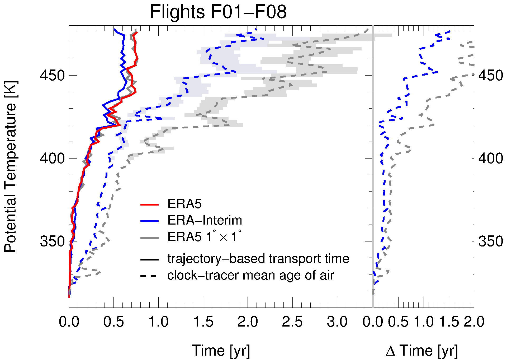
Figure 5 Trajectory-based mean transport time back to the monsoon of 2016 (same as in Fig. 4a) and the clock tracer mean age of air inferred from three-dimensional CLaMS simulations, both averaged as medians in 2 K intervals. The trajectory calculations are driven by three data sets (ERA-Interim, ERA5 and ERA5 $\mathrm{1}{}^{\circ }\times \mathrm{1}{}^{\circ }$). The mean age of air is only available for three-dimensional CLaMS simulations driven by ERA-Interim and ERA5 $\mathrm{1}{}^{\circ }\times \mathrm{1}{}^{\circ }$. The time differences (Δ time) between the clock tracer mean age of air and the trajectory-based mean transport time are shown in the right panel. Methodological differences in calculating the mean age of air (Sect. 3.3) are indicated as shading (in light blue and light grey). The left envelope represents the age-spectrum-based mean age, and the right envelope represents the spectrum-based mean age including the tail correction (below 400 K, the difference between the three methods is minor and therefore not shown).

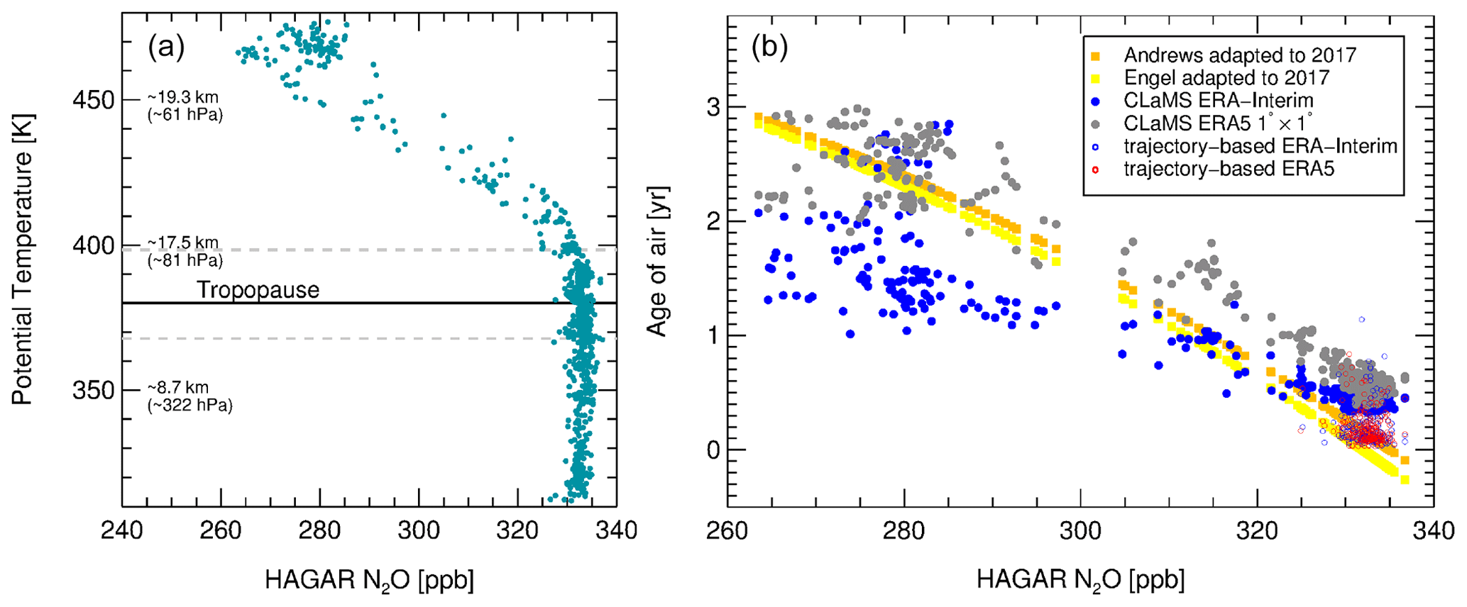
Figure 6 Airborne N₂O measurements from the StratoClim campaign in Kathmandu (Nepal) during July and August 2017 (a). In addition, the mean WMO tropopause using ERA5 (Hoffmann and Spang, 2022) and the lowest and highest tropopause (dashed grey lines) over Kathmandu during the flight days are shown. Mean age versus N₂O from Andrews et al. (2001) and Engel et al. (2002) adapted to the year 2017 compared to clock tracer mean age of air derived from global three-dimensional CLaMS simulations driven by ERA-Interim and and ERA5 $\mathrm{1}{}^{\circ }\times \mathrm{1}{}^{\circ }$ reanalysis (b). Only N₂O measurements from the HAGAR instrument above 375 K potential temperature are shown. Further, trajectory-based transport times using ERA5 and ERA-Interim (back to 1 June 2016) are added for potential temperature levels between 375 and 400 K.

N₂O profiles measured during the StratoClim campaign indicate strong mixing with older stratospheric air above ∼ 400 K (Fig. 6a; a more detailed discussion can be found in (Vogel et al., 2023)). Halon-1211 (which has a shorter lifetime than N₂O) measurements aboard Geophysica (see Fig. 2 in Adcock et al., 2021) indicate that, just below ∼ 400 K, a minor impact of older air is found. This is in agreement with the CLaMS backward trajectory calculations, which result in a BL fraction of a few percent below 100 % at these levels of potential temperature (Fig. 4a). Mixing with older stratospheric air above ∼ 400 K is evident in both the trajectory-based mean transport time and the mean age of air inferred from three-dimensional CLaMS simulations.

However, there is a strong difference between the used ECMWF reanalyses, as already found in trajectory-based mean transport times at potential temperatures higher than 410 K. ERA-Interim results in a mean age of about 2 years, while using ERA5 $\mathrm{1}{}^{\circ }\times \mathrm{1}{}^{\circ }$ yields a mean age of more than 3 years at 470 K (Fig. 5). The differences from using ERA-Interim and ERA5 $\mathrm{1}{}^{\circ }\times \mathrm{1}{}^{\circ }$ are much larger than from methodological differences for calculating the mean age of air (the clock tracer mean age, age-spectrum-based mean age and spectrum-based mean age including the tail correction; see Sect. 3.3).

Below 400 K potential temperature, there is a difference between the trajectory-based mean transport time and the mean age of air of ≈ 80 and ≈ 130 d using ERA-Interim or ERA5 $\mathrm{1}{}^{\circ }\times \mathrm{1}{}^{\circ }$, respectively. Moreover, trajectory-based transport times are restricted to below about 1 year (1 June 2016), which basically excludes the influence of downward transport from the stratosphere. However, due to the calculation of the mean value of the transport times of many single trajectories, this statistical treatment represents mixing between different air masses.

The three-dimensional CLaMS simulations (see Sect. 3.3) used here to calculate the mean age of air also include parameterised small-scale mixing (dependent on the deformation rate in the large-scale flow), which causes an additional ageing of air compared to the pure trajectory calculations (e.g. Konopka et al., 2019). However, it is also the case that differences in the treatment of the lower model boundary could cause the difference between the trajectory-based mean transport time and the mean age of air from global CLaMS simulations below 400 K (see Fig. 5). The age of air tracer is released in the lowest model layer, whereas the trajectory-based mean transport time is related to the top of the model boundary layer (ζ=120 K ∼ 2–3 km above surface following orography).

To validate the clock tracer mean age of air, as well as trajectory-based transport times from CLAMS, we use N₂O measured by the HAGAR instrument during the StratoClim research flights. We compute the mean age of air (Γ) from measured N₂O using Γ – N₂O correlations by Andrews et al. (2001) and Engel et al. (2002) based on aircraft and balloon measurements. We use Eq. (3) by Andrews et al. (2001), derived for N₂O mixing ratios of the year 1997:

$$\begin{array}{}\text{(1)}& \begin{array}{rl}\mathrm{\Gamma }& =\mathrm{0.0566}\times (\mathrm{313}-{\mathrm{N}}_{\mathrm{2}}\mathrm{O}[\mathrm{1997}\left]\right)-\mathrm{0.000195}\\ & \times (\mathrm{313}-{\mathrm{N}}_{\mathrm{2}}\mathrm{O}[\mathrm{1997}]{)}^{\mathrm{2}}.\end{array}\end{array}$$

This Γ – N₂O correlation is adapted to N₂O mixing ratios (in ppb) for the year 2017 as follows:

$$\begin{array}{}\text{(2)}& {\mathrm{N}}_{\mathrm{2}}\mathrm{O}\left[\mathrm{1997}\right]={\mathrm{N}}_{\mathrm{2}}\mathrm{O}\left[\mathrm{2017}\right]\times (\mathrm{313}/\mathrm{335}).\end{array}$$

In addition, the mean age of air is calculated using a correlation by Engel et al. (2002), which is based on measurements from 1997 and 2000 and is also adapted to N₂O mixing ratios for the year 2017.

$$\begin{array}{}\text{(3)}& \begin{array}{rl}\mathrm{\Gamma }& =\mathrm{6.03}-\mathrm{0.0136}\times {\mathrm{N}}_{\mathrm{2}}\mathrm{O}\left[\mathrm{1997}\right]+\mathrm{8.5892}\times {\mathrm{10}}^{-\mathrm{5}}\\ & \times {\mathrm{N}}_{\mathrm{2}}\mathrm{O}[\mathrm{1997}{]}^{\mathrm{2}}-\mathrm{3.376968}\times {\mathrm{10}}^{-\mathrm{7}}\times {\mathrm{N}}_{\mathrm{2}}\mathrm{O}[\mathrm{1997}{]}^{\mathrm{3}}\end{array}\end{array}$$

Figure 6b shows the Γ – N₂O correlations (valid above 375 K) from Andrews et al. (2001) and Engel et al. (2002) compared to the clock tracer mean age of air derived from global three-dimensional CLaMS simulations driven by ERA-Interim and ERA5 $\mathrm{1}{}^{\circ }\times \mathrm{1}{}^{\circ }$ reanalyses. In the Asian monsoon region, the clock tracer mean age of air based on ERA-Interim is lower than observation-based estimates, while the mean age of air based on ERA5 $\mathrm{1}{}^{\circ }\times \mathrm{1}{}^{\circ }$ is somewhat older but a little closer to the observations. For N₂O larger than ∼ 310 ppb (between 380 and 410 K), the simulated mean age of air for both ERA5 $\mathrm{1}{}^{\circ }\times \mathrm{1}{}^{\circ }$ and ERA-Interim is somewhat older than the observation-based mean age of air, likely related to an underestimation of subgrid-scale convective transport processes in the model (see Konopka et al., 2019, and discussion above).

Measured N₂O profiles indicate strong mixing with older stratospheric air only above ∼ 400 K (Fig. 6a); therefore, we can also compare trajectory-based transport times with the observation-based mean age of air below 400 K. In Fig. 6b, trajectory-based mean transport times (back to 1 June 2016) for potential temperature levels between 375 and 400 K are added. At these altitudes, a very good agreement between the observation-based mean age of air and trajectory-based transport times is found using both ERA-Interim and ERA5 to drive the trajectories. Therefore, CLaMS back trajectories are very well suited to CO₂ reconstruction, in particular below 400 K (Sect. 4.4). The CLaMS mean age of air above 400 K will be further used for comparison to observation-based mean ages from HFC-125 and C₂F₆, which are used to derive ascent rates (Sect. 4.3) .

4.2 Air mass origin and its vertical propagation

For a better source attribution of the StratoClim aircraft measurements, it is important to identify the source regions at the model BL. During the monsoon of 2017, most air parcels were released in the northern part of the Indian subcontinent, the Tibetan Plateau, the Bay of Bengal and eastern China (Fig. 7); however, the details differ between the three data sets. Using ERA-Interim, in general, more marine sources are found in the western Pacific compared to ERA5 for the monsoon of 2017. A cluster of air parcels at the model BL is found over the western Pacific, caused by typhoon activity at ∼ 20^∘ N and 125^∘ E influencing research flight F08 (Fig. A1) using ERA5 reanalysis (for details, see (Stroh and StratoClim-Team, 2023)), whereas this typhoon signature is not found using ERA-Interim and is only very weakly represented in ERA5 $\mathrm{1}{}^{\circ }\times \mathrm{1}{}^{\circ }$. Due to the better representation of convection, a slightly higher fraction of air is transported during the monsoon of 2017 from the model BL using ERA5 (64 %) compared to ERA-Interim (63 %) and ERA5 $\mathrm{1}{}^{\circ }\times \mathrm{1}{}^{\circ }$ (63 %). The frequency distributions for each research flight (F01–F08) for the monsoon of 2017 using ERA5 are shown in Fig. A1 in the Appendix.

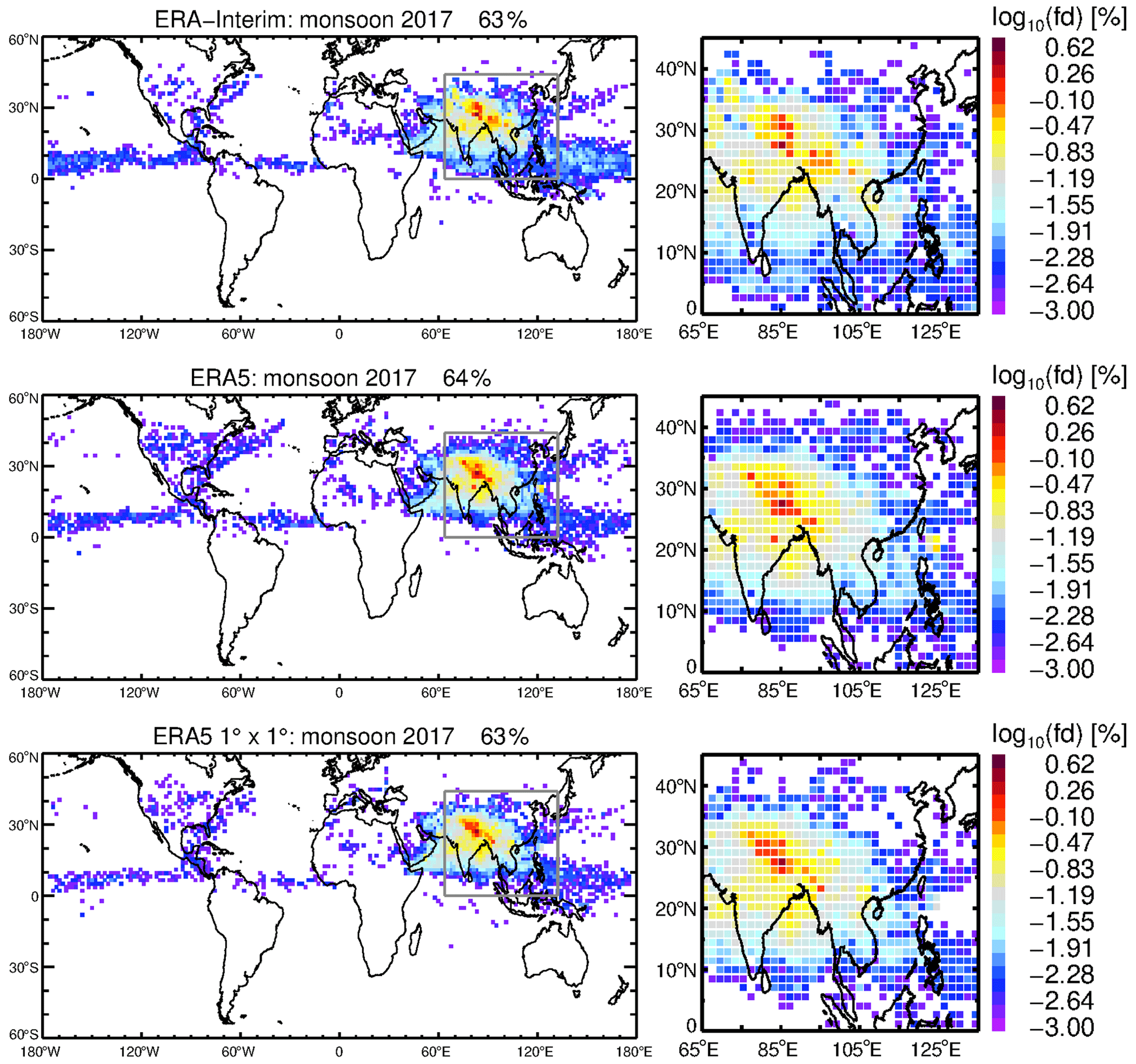
Figure 7 Frequency distribution (number of trajectories normalised by the total number of trajectories started along the flight path) of the locations where air parcels were traced back to the model BL. Trajectories driven by ERA-Interim, ERA5 and ERA5 $\mathrm{1}{}^{\circ }\times \mathrm{1}{}^{\circ }$ reanalysis were started along the complete flight tracks (every 1 s) of all eight Geophysica research flights. The frequency distributions are shown for the monsoon of 2017 (a zoom of Asia marked with a grey box is shown right beside). The frequency distribution is calculated in latitude–longitude bins of $\mathrm{1.5}{}^{\circ }\times \mathrm{2.0}{}^{\circ }$. The percentages indicate the fraction of air parcels released at the model BL within the monsoon of 2017. In summary, using ERA5 (ERA-Interim), 90 % (93 %) of the air parcels were released at the model BL after 1 June 2016, and the other 10 % (7 %) originated from aged air. The detailed pattern of the frequency distribution depends on the used reanalyses.

During pre-monsoon 2017 the origins are shifted towards the tropics to the northern Inter-Tropical Convergence Zone (ITCZ), e.g. over the Indian Ocean and the western Pacific (see Fig. A2 in the Appendix). For winter 2016–2017, the origins move further to the south to the southern Inter-Tropical Convergence Zone (ITCZ), mostly over the Warm Pool region, northern Australia and western Pacific. The contributions from post-monsoon 2016 and the monsoon of 2016 are minor. Differences between ERA5 and ERA-Interim are obvious in terms of transport time; e.g. during pre-monsoon 2017 and winter 2016–2017, 25 % of air is from the model BL using ERA-Interim, and only 20 % is from the model BL using ERA5. Thus, faster ERA-Interim vertical velocities in the UTLS (as already shown in Fig. 4) have an impact on the spatial distribution of the air mass origin in the model BL and yield differences between ERA-Interim and ERA5. During pre-monsoon 2017, the highest frequency distributions using ERA5 are found in the Bay of Bengal, whereas in ERA-Interim, high fractions are found in continental Asia, the Bay of Bengal and the tropical western Pacific.

Due to the different vertical velocities in ERA-Interim, ERA5 and ERA5 $\mathrm{1}{}^{\circ }\times \mathrm{1}{}^{\circ }$ (Fig. 4), the propagation of air masses from different model BL regions into the lower stratosphere varies in the region of the Asian monsoon. To infer these differences, the regional mask (Fig. 3) introduced in Sect. 3.2 is applied. Figure 8 shows the fraction of air from the model BL, split into the BL regions (Fig. 3), as well as the fractions of the free atmosphere using three data sets. The fractions of air are accumulated back to starting times of different seasons: monsoon 2017 (a), pre-monsoon 2017 (b), winter 2016–2017 (c), post-monsoon 2016 (d) and monsoon 2016 (e). The longer the trajectories, the higher the contributions from the model BL and the lower the fractions from the free atmosphere. The quality of the reconstruction of CO₂ depends on the trajectory length; therefore, it is important to know the contributions from the model BL in each altitude. The trajectory length can be too short (and thus miss contributions from the model BL) or too long (resulting in higher uncertainties) (for a detailed discussion on this issue see Vogel et al., 2023).

Figure 8 The fraction of air from the model boundary layer (BL) and the free atmosphere. The fraction from the model BL and from the free atmosphere is calculated from all backward trajectories started along the Geophysica flight tracks averaged in 2 K intervals and accumulated back to the start times of different seasons (rows), namely monsoon 2017, pre-monsoon 2017, winter 2016–2017, post-monsoon 2016 and monsoon 2016 (detailed start times are listed in Table 1) and for three data sets (ERA-Interim, ERA5 and ERA5 $\mathrm{1}{}^{\circ }\times \mathrm{1}{}^{\circ }$; columns). The fraction of air for monsoon 2016 (last row), referred to as the free atmosphere, corresponds to the fraction of aged air defined in Table 1. The fraction of air from the model BL is divided in the different BL regions as shown in Fig. 3.

Below 380 K, in general, the contribution from continental regions (Indian subcontinent, Bangladesh, Tibetan Plateau and the continental Northern Hemisphere) are higher using ERA5 compared to ERA-Interim (Fig. 9). While using ERA-Interim, higher contributions from the marine Northern Hemisphere and the Warm Pool region are found in these levels of potential temperature. Between 380 and 420 K, the contributions are vice versa, and more marine sources (marine Northern Hemisphere, Warm Pool region) are found using ERA5 compared to using ERA-Interim. In particular, above 430 K, the impact of the tropical Southern Hemisphere is much stronger in ERA-Interim compared to ERA5 (Fig. 9).

Using ERA5 $\mathrm{1}{}^{\circ }\times \mathrm{1}{}^{\circ }$ data to drive the CLaMS trajectories yields comparable results using ERA5 reanalysis (Figs. 8 and 9), and differences between ERA5 and ERA5 $\mathrm{1}{}^{\circ }\times \mathrm{1}{}^{\circ }$ are, in general, much lower than 10 percentage points in contrast to differences between ERA5 and ERA-Interim (∼ 20 percentage points).

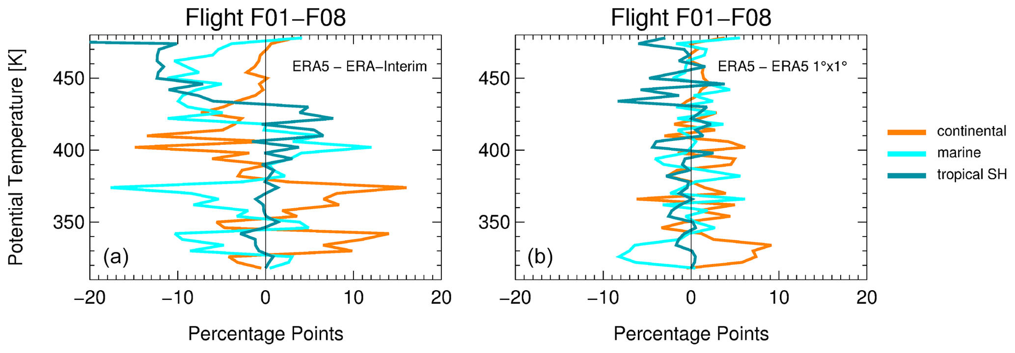
Figure 9 The difference in the fraction of air from the model boundary layer (BL) between back trajectories driven by ERA5 and ERA-Interim (a), as well as between back trajectories driven by ERA5 and ERA5 $\mathrm{1}{}^{\circ }\times \mathrm{1}{}^{\circ }$ (b), depending on potential temperature. The difference is accumulated back to monsoon 2016 (1 June 2016), and fractions are averaged in 4 K intervals in contrast to Fig. 8 (last row, where 2 K intervals are used) to highlight the main impact of the BL sources (however, the values of percentage points depends on the used averaging interval). The model boundary layer regions (Fig. 3) are summarised into three regions: continental (India, BGD, TIB, cNH) and marine regions (mNH, Wpool), mainly from the Northern Hemisphere and the tropical Southern Hemisphere (tSH).

Using cloud top altitudes from geostationary satellites to identify convection which occurred 30 d before the StratoClim measurements, Bucci et al. (2020) (see Fig. 10 therein) found that, up to an altitude of 17 km (∼ 400 K), convective sources contribute more than 95 % to the composition of the air probed during all flights. However, they calculate back trajectories only back to cloud top altitudes. Nevertheless, in CLaMS trajectories, only the convection inherent in the ERA5 and ERA-Interim reanalyses is included, and therefore, small scale convection could be underestimated. Further, in Bucci et al. (2020), only very young air masses (younger than 30 d) are considered; therefore, contributions from pre-monsoon 2017 and winter 2016–2017 are not covered. A more detailed comparison between the approach used in Bucci et al. (2020) and our analysis can be found elsewhere (Stroh and StratoClim-Team, 2023).

4.3 Effective ascent rates and transport time distribution

From CLaMS trajectories, effective ascent rates are calculated as the difference in potential temperature along the backward trajectories for a time interval of 1 and 20 d before the time of the aircraft measurements. The effective ascent rate is an integrated quantity, depends on time and is not an instantaneous ascent rate at a specific location in the atmosphere. The effective ascent rates are calculated for the three data sets (ERA-Interim, ERA5 and ERA5 $\mathrm{1}{}^{\circ }\times \mathrm{1}{}^{\circ }$; see Fig. 10). Negative effective ascent rates reflect the descent of air masses just before the flight, such as descending air from the lower stratosphere mixing into the air of the Asian monsoon anticyclone.

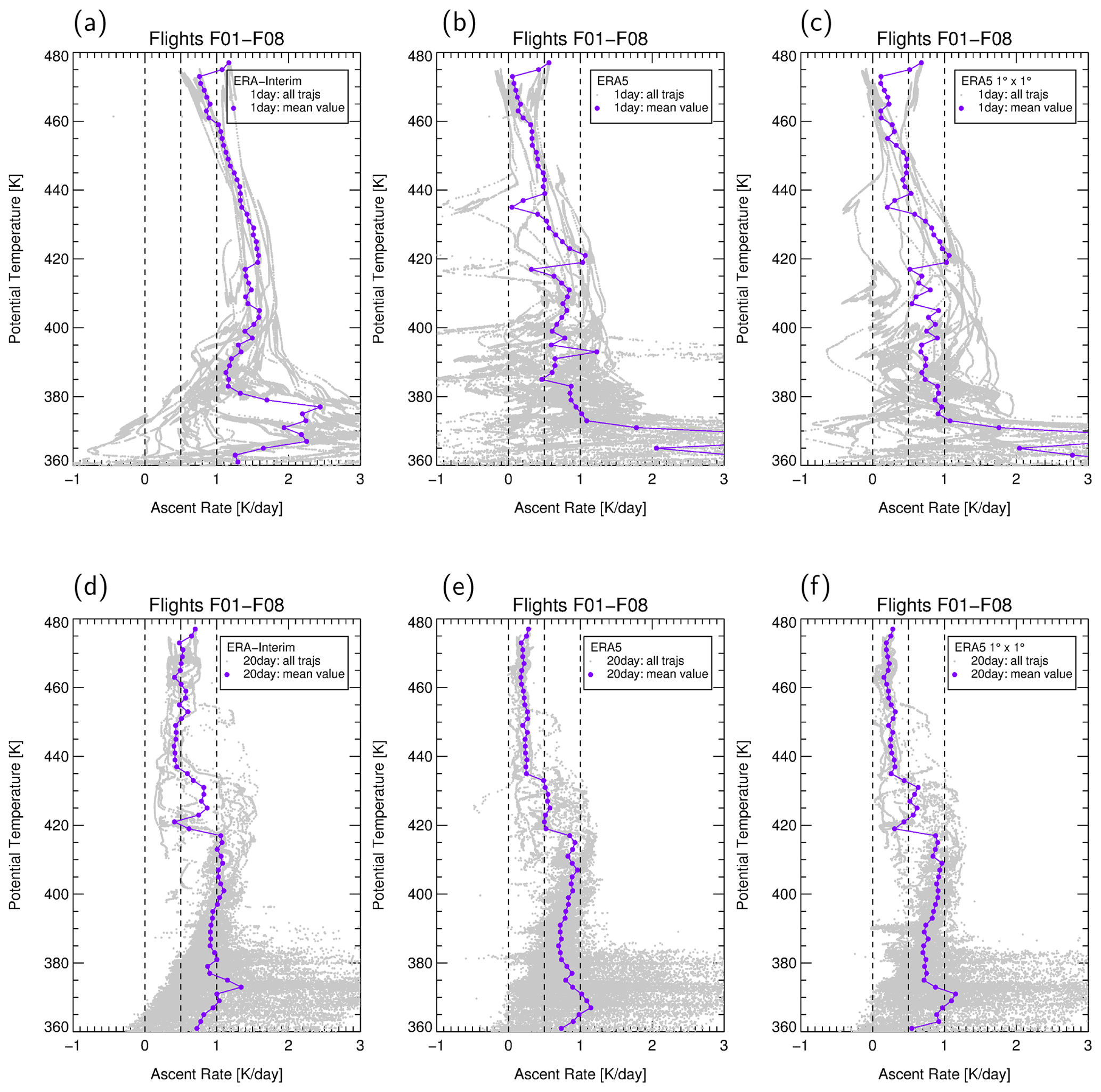
Figure 10 Effective ascent rates calculated as difference in potential temperature along backward trajectories driven by three data sets (ERA-Interim, ERA5 and ERA5 $\mathrm{1}{}^{\circ }\times \mathrm{1}{}^{\circ }$) to the time of the StratoClim measurements for a time interval of 1 d (a–c) and 20 d (d–f) and their mean values in 2 K intervals. The ascent rates are calculated for all trajectories calculated for research flights F01–F08. Negative effective ascent rates reflect the descent of air masses.

The effective ascent rates calculated over 24 h just before the aircraft measurements (1 d) reflect the short-term evolution of the sampled air mass and can be impacted by recent convective events (e.g. Fig. 10b at 390 K) or stratospheric intrusions, i.e. mixing with older stratospheric air (Fig. 10b at ∼ 415 and ∼ 435 K). Therefore, strong differences between the three data sets are found (Fig. 10a–c). Less impact by convection and stratospheric intrusions is found in ERA-Interim and in ERA5 $\mathrm{1}{}^{\circ }\times \mathrm{1}{}^{\circ }$. Below 360 K, effective ascent rates over 1 d up to ∼ 50 K d⁻¹ in ERA5, up to ∼ 30 K d⁻¹ in ERA5 $\mathrm{1}{}^{\circ }\times \mathrm{1}{}^{\circ }$ and only up to ∼ 20 K d⁻¹ are found (not shown here).

The mean effective ascent rates over 20 d (Fig. 10d–f) reflect a time-averaged ascent rate which is impacted by (vertical and horizontal) mixing of air masses of different origins and ages. In general, the mean effective ascent rates inferred from ERA-Interim are higher compared to ERA5 and ERA5 $\mathrm{1}{}^{\circ }\times \mathrm{1}{}^{\circ }$. To evaluate the mean effective ascent rates calculated from CLaMS back trajectories, mean ascent rates from air samples collected with the whole-air sampler (WAS) of Utrecht University are estimated using measurements of the long-lived trace gases HFC-125 and C₂F₆. Both trace gases are chemically inert in the troposphere and stratosphere and have been demonstrated to be suitable to derive observation-based mean age ages of air as both have very long atmospheric lifetimes (HFC-125 > 800 years (Leedham Elvidge et al., 2018) and C₂F₆ ≈ 10 000 years Worton et al., 2007). As the concept of age of air inferred from measurements only works in the stratosphere, a reference level of 390 K (corresponding to a mean age of 0 as determined via polynomial fit functions; Fig. 11) is used.

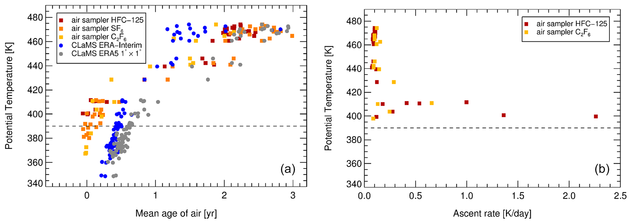
Figure 11 Observation-based mean age of air (a) and observation-based mean ascent rates above 390 K (b) derived from trace gas measurements of air samples collected with the whole-air sampler (WAS) of Utrecht University during the eight StratoClim research flights over the Indian subcontinent in summer 2017. Note that negative observation-based mean ages of air (< −0.1 year) found below 390 K are not shown. In addition, the clock tracer mean age of air for each air sample is shown derived from global three-dimensional CLaMS simulations driven by the ERA-Interim and ERA5 $\mathrm{1}{}^{\circ }\times \mathrm{1}{}^{\circ }$ reanalysis (b).

The observation-based mean age of air based on HFC-125 and C₂F₆ at 470 K is about ∼ 2–2.5 years (Fig. 11); the clock tracer mean age of air inferred from three-dimensional CLaMS simulations driven by ERA-Interim is younger than 2 years and ∼ 2–3 years using ERA5 $\mathrm{1}{}^{\circ }\times \mathrm{1}{}^{\circ }$ at this altitude (Fig. 11). The observation-based mean age of air inferred from HFC-125 and C₂F₆ is based on a reference level of 390 K, while the clock tracer mean age of air is based on Earth's surface. From trajectory-based transport times, a time lag of about 2–3 months between Earth's surface and 390 K can be estimated. Taking this time lag into account, the mean age of air driven by ERA-Interim is too young at this altitude, whereas the mean age of air from ERA5 $\mathrm{1}{}^{\circ }\times \mathrm{1}{}^{\circ }$ is somewhat too old at 470 K. Further, the observation-based mean age of air based on SF₆ is compared to the observation-based mean age of air based on HFC-125 and C₂F₆ (Fig. 11); however, the observation-based mean age of air based on SF₆ is about half a year older at 470 K compared to HFC-125 and C₂F₆, as caused by SF₆ sources in Asia (Adcock et al., 2021). Therefore, SF₆ is a rather unsuitable chemical age tracer for the Asian monsoon region.

The mean ascent rate for each air sample is simply derived from dividing the potential temperature difference in relation to the reference level of 390 K by the age of air derived from the two tracers (Fig. 11). The mean age of air reflects an integrated three-dimensional transit time, impacted by vertical and horizontal transport, as well as mixing processes. These processes are likely to be increasingly influential the further away the air is from the 390 K reference surface, with a clear tendency to increase the observation-based mean age of air because of the horizontal transport (in-mixing) of aged stratospheric air. In the trajectory-based mean effective ascent for 20 d, vertical and horizontal transport, as well as mixing processes, are included and therefore comparable with observation-based ascent rates.

Between 390 and 430 K, there is a variability of the mean effective ascent rates derived from HFC-125 and C₂F₆ from 0.2 up to 2.3 K d⁻¹. Above 430 K, the observation-based ascent rate converges to ∼ 0.2 K d⁻¹. Here, the mean effective ascent rate derived from ERA5 (as well as ERA5 $\mathrm{1}{}^{\circ }\times \mathrm{1}{}^{\circ }$) back trajectories over a time interval of 20 d (∼ 0.2–0.3 K d⁻¹) is in good agreement with observation-based mean ascent rates derived from air samples collected by the whole-air sampler. Mean effective ascent rates derived from ERA-Interim back trajectories are much faster (≈ 0.5 K d⁻¹) above 430 K.

Our analysis agrees with previous studies that found consistently that, in general, the vertical velocities in ERA-Interim are too fast in the tropics (Dee et al., 2011; Ploeger et al., 2012; Schoeberl et al., 2012). In addition, our findings show that the mean effective ascent rates of ∼ 0.2–0.3 K d⁻¹ derived from ERA5 in the region of the Asian monsoon in the lower stratosphere (430–480 K) agree very well with observation-based mean ascent rates derived from long-lived trace gases.

We show that the ascent rates along CLaMS backward trajectories depend on the used ECMWF reanalyses. However, they further depend on the considered altitude range. Thus, in general, ERA-Interim in the UTLS is faster than ERA5. However, due to a better representation of convection, air masses can be uplifted faster, as well as up to higher levels of potential temperature, by convection when using the ERA5 reanalysis compared to ERA-Interim. These differences have an impact on the frequency distribution of the transport time of backward trajectories from the main convective outflow to the sample region (referred to as transport time distribution) at different levels of potential temperature using the three data sets.

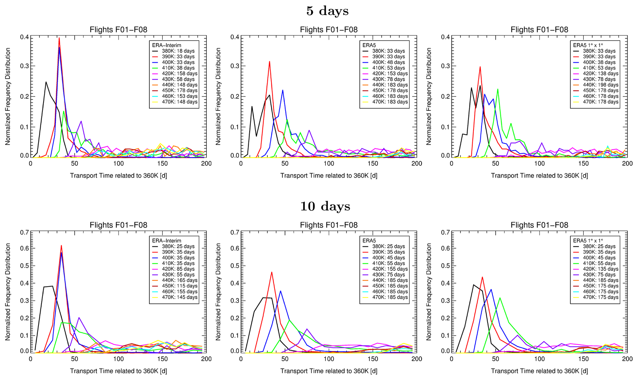
Figure 12 Normalised frequency distribution of the transport time from 360 K (≈ the level of maximum convective outflow) to the location of the aircraft measurement along the CLaMS backward trajectories (referred to as transport time distribution) using the three data sets (ERA-Interim, ERA5 and ERA5 $\mathrm{1}{}^{\circ }\times \mathrm{1}{}^{\circ }$). The transport time distribution is shown for different levels of potential temperature (for 2 K intervals) for a time resolution of 5 d (top) and 10 d (bottom). In the legend, the transport time to the maximum peak for each level of potential temperature is given.

Transport time distributions with a time resolution of 5 and 10 d using the three data sets (Fig. 12) reflect the faster vertical velocities found in the UTLS using ERA-Interim; thus, the maximum peak of the age spectrum is, in general, at shorter transport times compared to ERA5 and ERA5 $\mathrm{1}{}^{\circ }\times \mathrm{1}{}^{\circ }$. However, at lower potential temperatures, the impact of convection, which is different in the used reanalyses, has to be taken into account. Thus, the better representation of convection (visible in the two peaks at 380 K for a time resolution of 5 d; black line) and slower vertical velocities found in ERA5 in the UTLS can result in a spectrum peak at similar transit times compared to the maximum peak at a coarser resolution of convection and with faster vertical velocities found in ERA-Interim. Therefore, the maximum peaks for 390 and 400 K using ERA-Interim are at similar transport times.

4.4 Reconstruction of CO₂ from airborne measurements

Airborne CO₂ measurements from the StratoClim campaign in Kathmandu (Nepal) during July and August 2017 are shown in Fig. 13. Each air parcel is coloured by the trajectory-based transport time from the model BL to the time of measurements inferred by Lagrangian back trajectory calculations driven by ERA-Interim (Fig. 13a). Trajectory-based transport times increase with the altitude of sampled air parcels (as already shown in Fig. 4). However, there is also a strong variability of transport times between individual air parcels at the same level of potential temperature, indicating the mixing of air masses with different transport times or of different ages (Fig. 13a). Moreover, differences in the transport times of individual air parcels are found using ERA5 instead of ERA-Interim (Fig. 13b) reanalyses. In the stratosphere, ERA-Interim has the tendency to be faster (shorter transport times) than ERA5 (bluish data points). In the UTLS, certain air masses are found to experience faster upward transport by convection using ERA5 rather than ERA-Interim (reddish points).

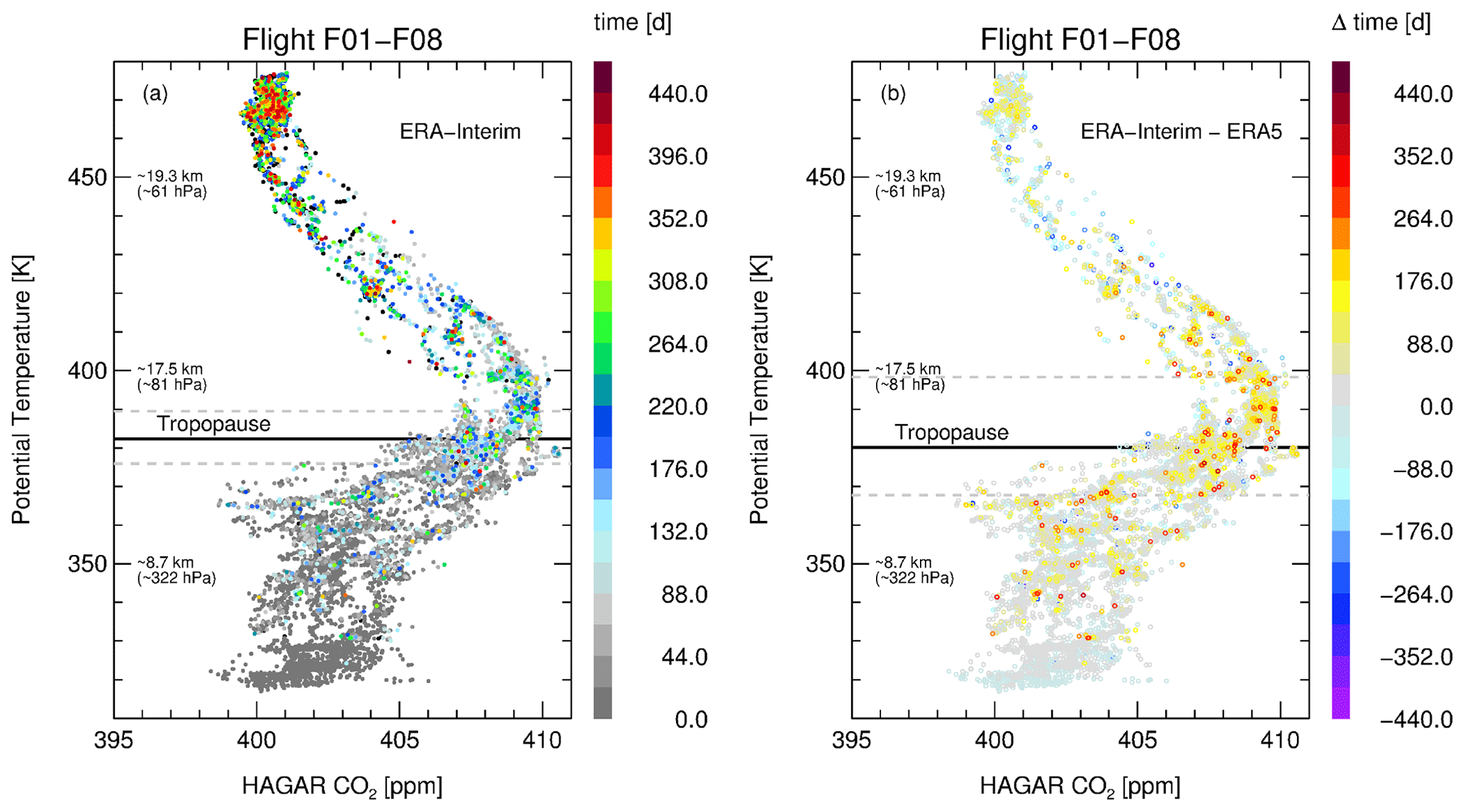
Figure 13 Airborne CO₂ measurements from the StratoClim campaign in Kathmandu (Nepal) during July and August 2017. Each air parcel is coloured by the trajectory-based transport time from the model boundary layer (BL) in relation to the time of measurements inferred by Lagrangian back trajectory calculations driven by ERA-Interim (a). Air parcels located in the model BL are not shown. Aged air (air located in the free atmosphere on 1 June 2016) is marked in black. Further, the differences in the trajectory-based transport time between ERA-Interim and ERA5 (b) are shown from back trajectories reaching the model BL. In addition, the mean WMO tropopause (Hoffmann and Spang, 2022) and the lowest and highest tropopause (dashed grey lines) over Kathmandu during the aircraft campaign (27 July–10 August 2017) are added using ERA-Interim (a) and ERA5 (b) reanalysis.

In addition, differences in the tropopause height (in particular for the local minimum and maximum) exist using ERA5 and ERA-Interim. Hoffmann and Spang (2022) found that the standard deviations in the tropical tropopause height are ≈ 30 %–50 % higher in ERA5 (T_L 639, high-resolution version) compared to ERA-Interim, mostly related to explicitly resolved gravity waves in ERA5, which are absent in ERA-Interim due to its coarser spatial resolution. Tegtmeier et al. (2020) attributed tropopause shifts between ERA-Interim and ERA5 to the higher vertical resolution of ERA5, having 3 times more levels in the tropical tropopause than ERA-Interim.

For a reliable reconstruction of measured vertical CO₂ profiles over the entire altitude range, both accurate back trajectory calculations and precise CO₂ concentrations at the ground are required. For the latter purpose, a regional mask was developed where CO₂ is prescribed in the model BL depending on different BL regions (Fig. 3).

To reconstruct vertical profiles of trace gases in the region of the Asian monsoon up to 410 K potential temperature, the fraction of air from the model BL has to be ∼ 100 %; otherwise, mixing with aged air has to be taken into account. In Sect. 4.1, it was shown that, using a trajectory length back to the start time of monsoon 2016 (≈ 10–14 months), a boundary layer fraction of about 100 % was reached up to 410 K. Above 410 K, mixing with older air masses successively occurred, and the fraction from the model BL rapidly decreased.

Figure 14a–c shows reconstructed CO₂ using three data sets for back trajectory calculations until 1 June 2016, neglecting the contributions from the free atmosphere (aged air). The comparison with measured in situ CO₂ profiles shows a good overall agreement from the model BL up to ∼ 410 K for ERA5 trajectories. A reconstruction using ERA-Interim shows a stronger dispersion between 390 and 420 K because, here, ERA-Interim vertical velocities are faster than ERA5. Further, below 370 K, the measured variability of CO₂ caused by convection (low CO₂ at ≈ 360 K) is better reproduced using ERA5 due to the better representation of convection. A CO₂ reconstruction using trajectories driven by ERA5 $\mathrm{1}{}^{\circ }\times \mathrm{1}{}^{\circ }$ is somewhere between ERA-Interim and ERA5.

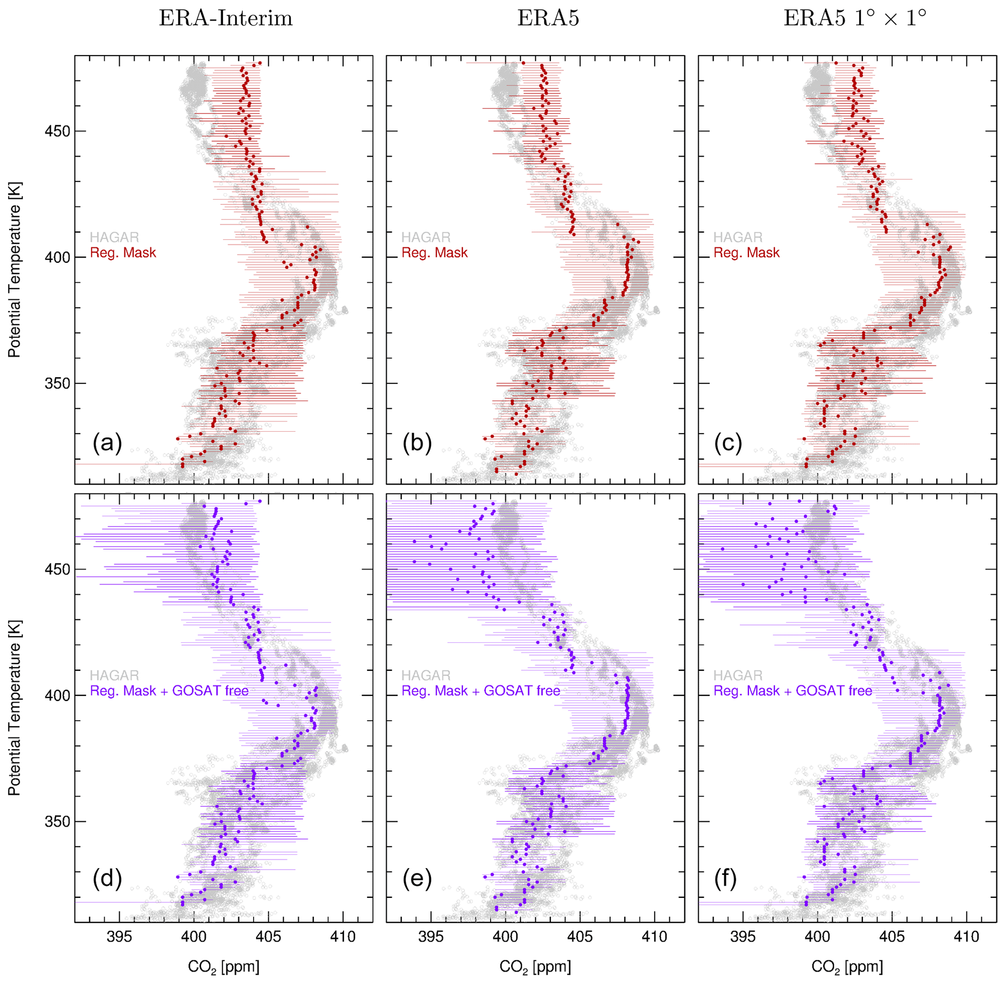
Figure 14 Reconstructed CO₂ using back trajectory calculations until 1 June 2016 driven by three data sets (ERA-Interim, ERA5 and ERA5 $\mathrm{1}{}^{\circ }\times \mathrm{1}{}^{\circ }$) compared to HAGAR CO₂ airborne measurements. Reconstructed CO₂ is shown using the regional mask shown in Fig. 3 for the fraction of trajectories ending in the model BL driven by the three data sets (a–c). Reconstructed CO₂ is shown as the median calculated from all trajectories until 1 June 2016 in 1 K intervals for research flights F01–F08. Reconstructed CO₂ is shown using, in addition, GOSAT-L4B CO₂ data for the fraction of trajectories ending in the free atmosphere, mainly from stratospheric background (d–f). Bars indicate the range between the 25th and 75th percentiles.

Above ∼ 410 K, aged air has to be taken into account, as discussed in Sect. 4.1. Figure 14d–f shows reconstructed CO₂ but using, in addition, GOSAT-L4B CO₂ data for the fraction of aged air. For back trajectories ending in the free atmosphere, CO₂ is reconstructed from GOSAT-L4B data that provide CO₂ values up to 10 hPa (for details, see Vogel et al., 2023). Here, for each 1 K interval, the median of all air parcels considering the fractions from both the model BL and the aged air is calculated. This approach allows the mixing of air at the top of the Asian monsoon anticyclone between air from the boundary layer and air from the (stratospheric) background to be considered.

Caused by too-fast vertical velocity in the UTLS in ERA-Interim (according to effective ascent rates inferred from whole-air sampler measurements), higher CO₂ from the model BL is found in the lower stratosphere. Even including the contribution of aged air from GOSAT-L4B data yields slightly higher reconstructed CO₂ above 420 K using ERA-Interim compared to the measurements. Using ERA5 and ERA5 $\mathrm{1}{}^{\circ }\times \mathrm{1}{}^{\circ }$ yields slightly lower reconstructed CO₂ above 420 K. However, above 410 K, the quality of the GOSAT-L4B also needs to be taken into account for an assessment of the quality of CO₂ reconstruction. GOSAT-L4B data depend on CO₂ fluxes at the Earth's surface (GOSAT-L4A data), on model resolution and on vertical transport in the used atmospheric transport model, which could have a too-fast transport in the lower stratosphere, similarly to ERA-Interim.

In summary, there are differences in CO₂ reconstruction using the three data sets, whereby the statistical variability of the CO₂ reconstruction is in the range of the measurements. A CO₂ reconstruction using ERA5 agrees best with the measured vertical CO₂ profile up to 410 K, although there is only a slight difference when using ERA-Interim reanalysis. It should be noted that the used CO₂ reconstruction technique has limitations because of the very low number of sites measuring ground-based CO₂ over the Indian subcontinent in 2016–2017. The UTLS is a very sensitive region with regard to the interplay between deep convection and vertical velocities in the lower stratosphere influencing the vertical transport of CO₂ and thus the CO₂ reconstruction using trajectory calculations.

5 Conclusions

It was reported previously that, because of a better spatial and temporal resolution, the ERA5 reanalysis yields a better representation of convection than the predecessor, ERA-Interim (e.g. Hoffmann et al., 2019; Li et al., 2020; Legras and Bucci, 2020; Malakar et al., 2020). Further, it was shown that the vertical transport in ERA-Interim is too fast in the tropical UTLS (Dee et al., 2011; Ploeger et al., 2012; Schoeberl et al., 2012; Tegtmeier and Krüger, 2022). At higher northern-hemispheric stratospheric levels above the tropical tropopause layer, it was reported that ERA5 transport is likely too slow (Ploeger et al., 2021). In general, our findings confirm these results; however, in our study, we focus in detail on the Asian summer monsoon region.

Differences in the transport of air in the region of the Asian summer monsoon of 2017 were inferred using the Chemical Lagrangian Model of the Stratosphere (CLaMS) driven by three data sets, namely two ECMWF reanalyses with different resolutions (ERA-Interim, ERA5 and ERA5 $\mathrm{1}{}^{\circ }\times \mathrm{1}{}^{\circ }$). The model results were assessed using unique airborne measurements up to ∼ 20 km (∼ 475 K) during the Asian summer monsoon of 2017, conducted with the Geophysica aircraft during the StratoClim campaign in Nepal (Stroh and StratoClim-Team, 2023). CLaMS diabatic backward trajectories were calculated for all Geophysica research flights (F01–F08) performed over the Indian subcontinent. Trajectory-based transport times, the origin of air at the Earth's surface, mean effective ascent rates, transport time distributions and the mean age of air from three-dimensional CLaMS simulations were compared using the three data sets.

Below 410 K, convection as represented in ERA5 yields faster trajectory-based upward transport (up to ≈ 20 d) than ERA-Interim. On the other hand, air masses above 420 K show trajectory-based transport times that are up to 2 months (≈ 60 d) shorter from the model BL to the UTLS in ERA-Interim compared to ERA5. A better representation of convection and slower vertical velocities above the convection found in ERA5 can yield similar transport times up to the UTLS (∼ 380–390 K) compared to a coarser resolution of convection and faster vertical velocities as found in ERA-Interim. Therefore, the frequency distribution of the transport time from the level of maximum convective outflow (∼ 360 K) to different levels of the aircraft measurement based on back trajectories (denoted as transport time distribution) are very sensitive to the three data sets.

Below 380 K, contributions from continental regions (Indian subcontinent, Bangladesh, Tibetan Plateau and the continental Northern Hemisphere) to air masses along the flight paths of all eight local research flights (F01–F08) are higher using ERA5 compared to ERA-Interim, while in ERA-Interim, higher contributions from the marine Northern Hemisphere and the Warm Pool region are found. Although using ERA-Interim for back trajectory calculations generally allows for more marine sources at these altitudes to be identified, the signal from typhoon activity in the western Pacific (in particular during research flight F08 on 10 August 2017) is not visible when using ERA-Interim. Above 380 K, it is the other way round, and more marine sources are found using ERA5, and a stronger impact of the tropical Southern Hemisphere is found using ERA-Interim.

Above 430 K, the mean effective ascent rates derived from ERA5 back trajectories over a time interval of 20 d (≈ 0.2–0.3 K d⁻¹) are in good agreement with the observation-based mean ascent rates inferred from long-lived trace gases such as C₂F₆ and HFC-125 derived from air samples collected by the whole-air sampler aboard Geophysica. Mean effective ascent rates derived from ERA-Interim back trajectories are much faster (≈ 0.5 K d⁻¹) than observation-based mean ascent rates at these altitudes. Caused by the difference in the mean effective ascent rates when using two ECMWF reanalyses, a different mean age of air is calculated at higher altitudes. At 470 K, a mean age of air of younger than 2 years is calculated using three-dimensional CLaMS simulations driven by ERA-Interim, while using ERA5 $\mathrm{1}{}^{\circ }\times \mathrm{1}{}^{\circ }$ results in a mean age between 2 and 3 years being calculated (a three-dimensional CLaMS simulation driven by ERA5 is not yet available). At these altitudes, the observation-based age of air from C₂F₆ and HFC-125 is up to ∼ 2–2.5 years. In the monsoon region, above 430 K, the mean age of air using the ERA-Interim mean age is, in general, too young, while ERA5 $\mathrm{1}{}^{\circ }\times \mathrm{1}{}^{\circ }$ is somewhat too old but closer to the observation-based age of air derived from N₂O compared to using ERA-Interim. Thus uncertainties regarding the correct simulation of the mean age of air in the lower stratosphere (430–480 K) still remain.

Trajectory-based transport times inferred from ERA5 $\mathrm{1}{}^{\circ }\times \mathrm{1}{}^{\circ }$ trajectories have, in principle, a similar behaviour compared to the times obtained using ERA5; however, the variability is somewhat different, caused by the reduced temporal and horizontal resolutions in ERA5 $\mathrm{1}{}^{\circ }\times \mathrm{1}{}^{\circ }$. Details in simulated transport, e.g. air mass origin, impact of tropical cyclones, transport time distribution and the vertical dispersion, are different when employing ERA5 and ERA5 $\mathrm{1}{}^{\circ }\times \mathrm{1}{}^{\circ }$. For long-term simulations over several years or decades, ERA5 $\mathrm{1}{}^{\circ }\times \mathrm{1}{}^{\circ }$ appears to be an acceptable (computing-time-saving) data set; however, for detailed transport calculations in the Asian monsoon region (e.g. analysing aircraft or balloon measurements), the full-resolution ERA5 reanalysis resolves more small-scale features and variability.

Further, high-resolution CO₂ profiles measured aboard Geophysica were reconstructed using ground-based measurements of CO₂ mainly from Nainital (northern India) from Lagrangian model simulations using three data sets (ERA-Interim, ERA5 and ERA5 $\mathrm{1}{}^{\circ }\times \mathrm{1}{}^{\circ }$), leading to an improved understanding of the vertical structure of CO₂ in the monsoon region. A reliable reconstruction (simulation) of vertical CO₂ profiles during the Asian monsoon is a challenge for model simulations because the seasonal variability of CO₂ at the ground, mixing with aged stratospheric air and the vertical velocities (including convection and vertical ascent caused by diabatic heating in the UTLS) have to be simulated accurately. Our analysis shows that, by using the ERA5 reanalysis for CO₂ reconstruction, a slightly better agreement with high-resolution in situ aircraft CO₂ measurements is obtained compared to using ERA-Interim. However, at higher altitudes (above 410 K), uncertainties remain in the used reconstruction approach, mainly caused by the limitations of the GOSAT-L4B CO₂ data used for characterising aged stratospheric air, demonstrating the need for better global CO₂ simulations. Further, a sufficiently dense coverage of continuous quality-controlled ground-based monitoring of CO₂ over the Indian subcontinent is a prerequisite for a reliable simulation of vertical CO₂ profiles in the region of the Asian summer monsoon.

Appendix A: Air mass origin and trajectory-based transport time

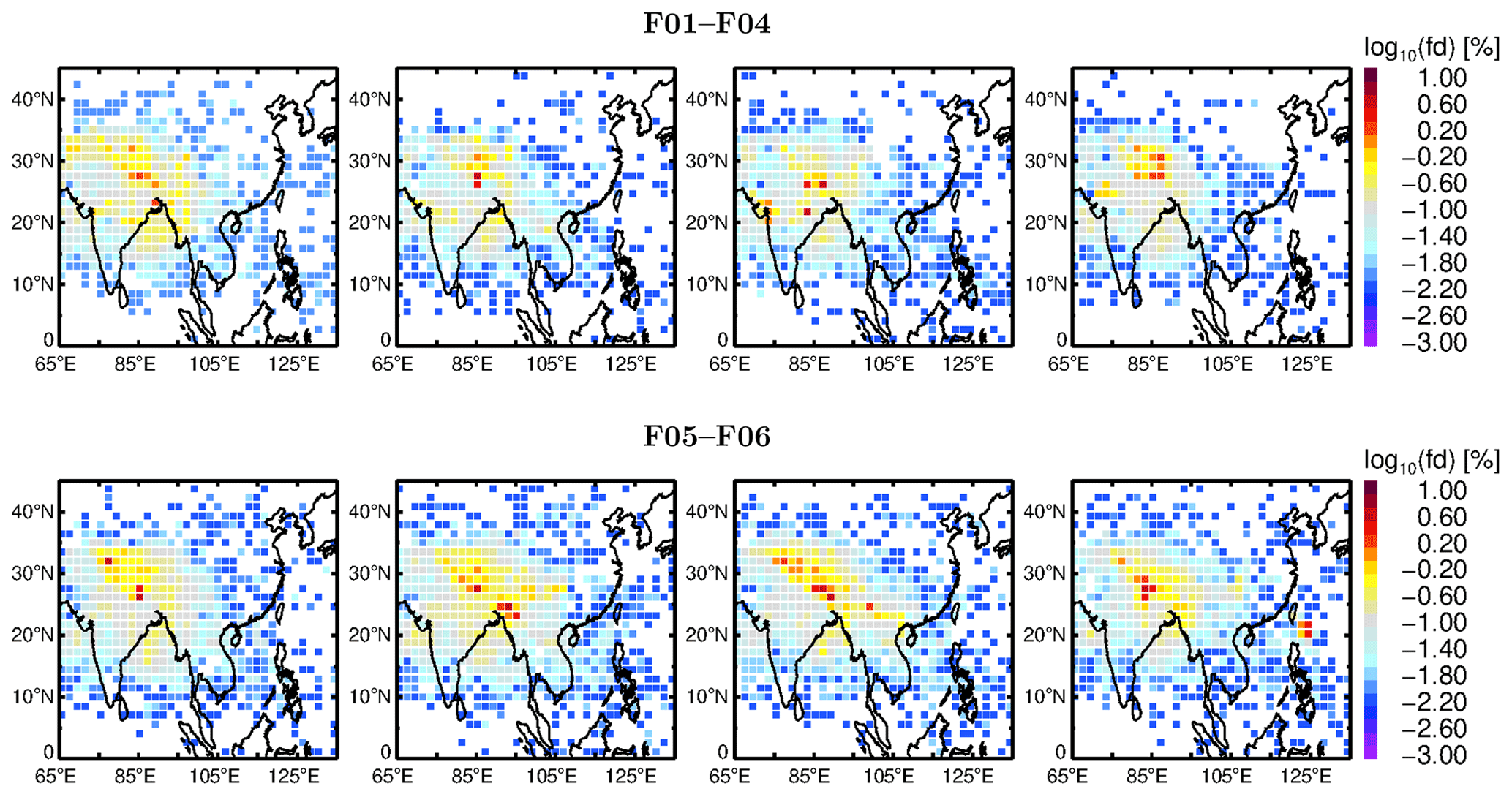
Figure A1 Frequency distribution (fd) of the air mass origins at the model boundary layer (BL) for each research flight (F01–F08) using ERA5 reanalysis for the monsoon season of 2017.

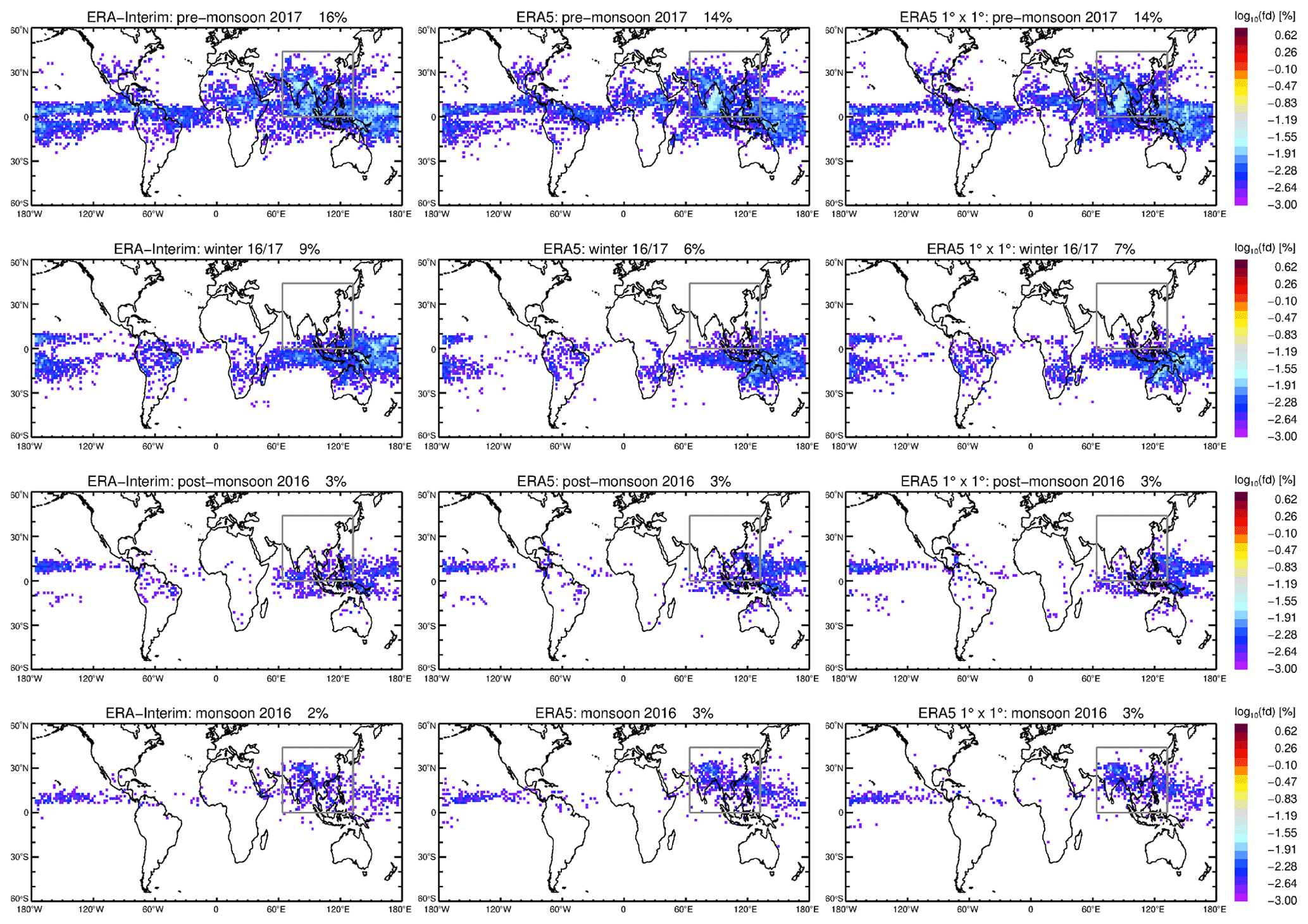
Figure A2 Frequency distribution (fd) of the air mass origins at the model boundary layer (BL), similarly to Fig. 7 but for pre-monsoon 2017, winter 2016–2017, post-monsoon 2016 and monsoon 2016. The percentages indicate the fraction of air parcels released at the model BL within a certain season. The detailed patterns of the frequency distribution depend strongly on the considered season, as well as on used three data sets (ERA-Interim, ERA5 and ERA5 $\mathrm{1}{}^{\circ }\times \mathrm{1}{}^{\circ }$).

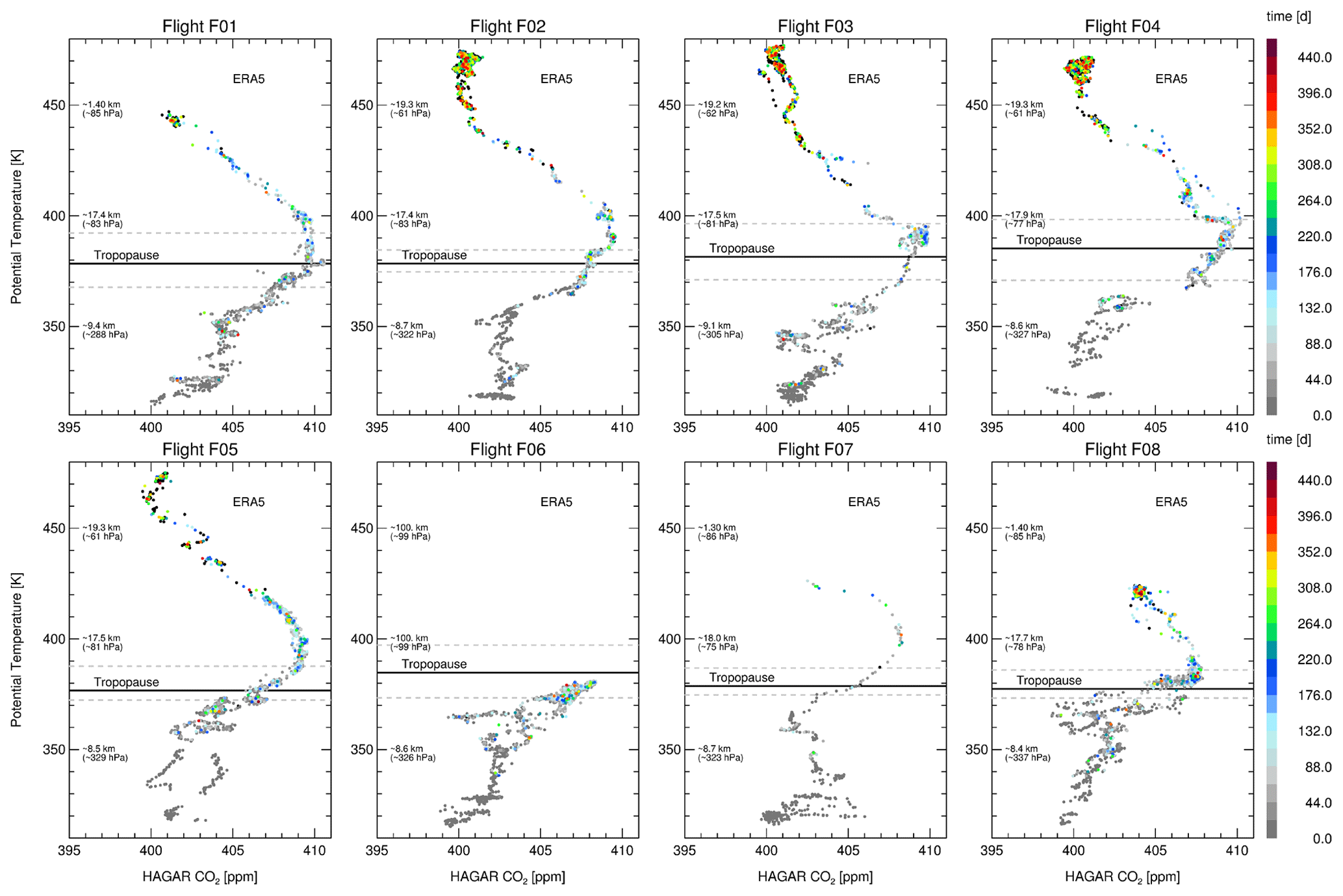
Figure A3 Airborne CO₂ measurements from the StratoClim campaign in Kathmandu (Nepal) and trajectory-based transport time for each research flight (F01–F08) using ERA5 reanalysis (similarly to Fig. 13 but for single flights). Each air parcel is coloured by the trajectory-based transport time from the model boundary layer (BL) to the time of measurements. Air parcels located in the model BL are not shown. Aged air (air located in the free atmosphere on 1 June 2016) is marked in black. In addition, the mean WMO tropopause (Hoffmann and Spang, 2022) and the lowest and highest tropopause (grey dashed lines) over Kathmandu on the day of the measurement are shown inferred from ERA5.