the Creative Commons Attribution 4.0 License.
the Creative Commons Attribution 4.0 License.
 | 12 Mar 2024
Influence of cloud retrieval errors due to three-dimensional radiative effects on calculations of broadband shortwave cloud radiative effect
Adeleke S. Ademakinwa
Zahid H. Tushar
Jianyu Zheng
Chenxi Wang
Sanjay Purushotham
Jianwu Wang
Kerry G. Meyer
Tamas Várnai
We investigate how cloud retrieval errors due to the three-dimensional (3D) radiative effects affect broadband shortwave (SW) cloud radiative effects (CREs) in shallow cumulus clouds. A framework based on the combination of large eddy simulations (LESs) and radiative transfer (RT) models was developed to simulate both one-dimensional (1D) and 3D radiance, as well as SW broadband fluxes. Results show that the broadband SW fluxes reflected at top of the domain, transmitted at the surface, and absorbed in the atmosphere, computed from the cloud retrievals using 1D RT (), can provide reasonable broadband radiative energy estimates in comparison with those derived from the true cloud fields using 1D RT (F1D). The difference between these 1D-RT-simulated fluxes (, F1D) and the benchmark 3D RT simulations computed from the true cloud field (F3D) depends primarily on the horizontal transport of photons in 3D RT, whose characteristics vary with the sun's geometry. When the solar zenith angle (SZA) is 5°, the domain-averaged values are in excellent agreement with the F3D, all within 7 % relative CRE bias. When the SZA is 60°, the CRE differences between calculations from and F3D are determined by how the cloud side-brightening and darkening effects offset each other in the radiance, retrieval, and broadband fluxes. This study suggests that although the cloud property retrievals based on the 1D RT theory may be biased due to the 3D radiative effects, they still provide CRE estimates that are comparable to or better than CREs calculated from the true cloud properties using 1D RT.
- Article
(4151 KB) - Full-text XML
- BibTeX
- EndNote


Covering about 60 %–70 % of the Earth's surface (Rossow and Schiffer, 1999; Vardavas and Taylor, 2011), clouds play a very important role in the Earth's climate system. Clouds can cool the Earth by reflecting shortwave (SW) solar radiative flux back to space and at the same time warm the Earth by retaining the outgoing longwave (LW) infrared radiative flux at the top of the atmosphere (TOA), known as cloud radiative effects (CREs). The annual global average TOA CRE is approximately −50 W m−2 at SW and 30 W m−2 at LW, resulting in a net CRE of about −20 W m−2 (Stocker et al., 2013). These strong CREs show that clouds greatly affect the Earth's energy budget (Ramanathan et al., 1989; Kiehl and Trenberth, 1997; Trenberth et al., 2009). The CRE of clouds is largely determined by the optical and microphysical properties of clouds including the cloud optical thickness (τ), cloud droplet effective radius (re), and cloud liquid water path (LWP). Thus, continuous measurements of these cloud properties from regional to global scales are critical to better understand the role of clouds in the climate systems. Currently, satellite-based remote sensing is the only way to make such observations. Remotely “retrieved” cloud properties based on these satellite observations are often used to derive the radiative effects of clouds (e.g., Wielicki et al., 1996; Platnick et al., 2003; Loeb and Manalo-Smith, 2005; Oreopoulos et al., 2016) and evaluate the simulations of Earth system models (ESMs) (Kay et al., 2012; Nam et al., 2012; Song et al., 2018).
A commonly used retrieval technique in passive satellite remote sensing is the bispectral retrieval method first developed by Nakajima and King (1990). It retrieves τ and re simultaneously from a pair of total reflectance measurements, one from the non-absorbing visible or near-infrared (VNIR) band (e.g., 0.66 µm) and the other from the moderately absorbing shortwave infrared (SWIR) band (e.g., 2.13 µm). Since clouds in reality have three-dimensional (3D) structures, the simulation of radiative transfer (RT) in clouds should ideally consider the transport of radiation in both vertical and horizontal directions (referred to as “3D RT”). Unfortunately, the computational cost for 3D RT is extremely high. As a result, operational bispectral cloud retrievals are almost exclusively based on the one-dimensional (1D) RT theory that considers only the vertical and ignores the net horizontal transport of radiation. The radiative properties of clouds under 3D RT are substantially different from those under 1D RT. This is known as the 3D radiative effects and can lead to substantial biases in cloud property retrievals based on 1D RT (Várnai and Marshak, 2002; Marshak et al., 2006; Zhang et al., 2012, 2016). Although recent efforts have been made to employ machine learning techniques to retrieve cloud properties based on 3D RT theory (Okamura et al., 2017; Masuda et al., 2019; Nataraja et al., 2022), these machine-learning-based algorithms are still in their infancy and far from being used in operational algorithms.
Many previous studies have investigated the 3D radiative effects on satellite radiance observations and cloud property retrievals. For example, Welch and Wielicki (1984) used some “toy” cloud fields (e.g., cubic and cylindrical) to illustrate the impact of side-illuminating and mutual shadowing on cloud albedo. Várnai and Davis (1999) and Várnai (2000) elucidated several 3D RT mechanisms, e.g., upward–downward trapping–escaping, that can result in significant differences between 1D and 3D cloud albedo. Hogan et al. (2019) proposed a distinct mechanism, named “entrapment”, which plays a key role in the 3D radiative effect of clouds. Davis and Marshak (2001) pointed out that the channeling effect in 3D RT can smoothen out the small-scale cloud variations and lead to the reduction of cloud brightness at cloud edges. Marshak et al. (2006) explained how the radiance biases due to 3D radiative effects can lead to τ and re retrieval biases in MODIS (Moderate Resolution Imaging Spectroradiometer) cloud products. This study is built upon these classic papers but has a different objective.
Here, we investigate an important question: do cloud property retrievals based on 1D RT, which are potentially biased due to the 3D radiative effects, still provide an observational basis to estimate the broadband SW CREs? This is an important question because as mentioned above, operational cloud retrieval products from, for example, MODIS, are frequently used for CRE estimation and ESM evaluation. However, to our best knowledge, the impacts of retrieval bias due to the 3D radiative effects on such applications have never been examined systematically in previous studies. To better explain our objective and the difference of this study from many previous ones on the 3D radiative effects, we need to introduce the framework illustrated in Fig. 1. As conceptually illustrated in Fig. 1, the observed radiances are inherently 3D (i.e., from Box A to C) because the RT in nature is 3D. However, when 1D RT theory is used to interpret the observations, we get the “retrieved cloud properties” in Box D that can be significantly different from the “true” cloud properties in Box A. Although the retrieved cloud properties are often biased due to the 3D radiative effects, they are still widely used to compute the radiative fluxes by clouds (i.e., from Box D to E) using 1D RT and the results are often used for studying the climatic effects of clouds (e.g., Kato et al., 2011; Zelinka et al., 2012; Oreopoulos et al., 2016). In contrast, the true radiative fluxes in nature are also 3D (i.e., from Box A to F). A few recent studies have computed and compared the 1D and 3D radiative fluxes as well as heating rates by clouds. For example, Barker et al. (2011, 2012) and Okata et al. (2017) compared the 1D and 3D SW fluxes computed based on the constructed A-Train cloud scenes at the TOA and surface. A more recent study by Singer et al. (2021) utilized large eddy simulation (LES) cloud fields of different cloud regimes to assess the SW radiative flux and TOA albedo bias associated with the 3D effects. The main difference between their study and this current work is as follows: they compared the 3D (i.e., Box F in Fig. 1) with the 1D broadband fluxes (i.e., Box G in Fig. 1) both computed from the true clouds. In contrast, we argue that the true clouds are not known in practice and therefore we compare the 3D flux (i.e., Box F in Fig. 1) with the 1D flux computed from the retrieved cloud properties (i.e., Box E in Fig. 1); this approach enables us to measure the impact of cloud retrieval errors on the radiative flux and CRE.
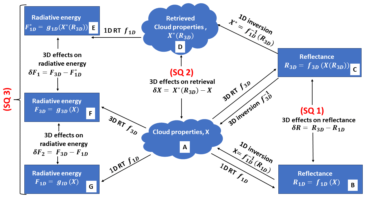
Figure 1Conceptual framework to understand the study. R3D and R1D are the reflectances from three-dimensional (3D) and one-dimensional (1D) radiative transfer (RT), respectively, while δR is their difference. X represents the true cloud field and X∗(R3D) represents the retrieved cloud properties from 3D RT reflectance, while δX is the cloud property retrieval bias. and F1D are the radiative flux calculated using 1D RT on the retrieved cloud properties and true cloud properties, respectively. F3D is the radiative flux derived from the true cloud field using 3D RT. δF1 and δF2 are the differences between the pairs (, F3D) and (F1D, F3D), respectively.
To determine whether biased cloud retrievals of cloud properties can still provide an observational basis for CREs, we focus on three important scientific questions (SQs) as illustrated in Fig. 1.
-
SQ 1: how does the reflectance simulated based on 3D RT (R3D) compare with the reflectance simulated based on 1D RT (R1D) for different types of clouds at different illuminating–viewing geometries (i.e., comparing Box C to B in Fig. 1)?
-
SQ 2: how do the retrieved cloud properties, e.g., cloud optical thickness and cloud droplet effective radius derived from the 3D reflectance using 1D RT, compare to the true cloud properties (i.e., comparing Box D to A in Fig. 1)?
-
SQ 3: comparing δF1 to δF2 in Fig. 1, i.e., how are the broadband SW radiative fluxes derived from the retrieved cloud properties using 1D RT () (see Box E in Fig. 1) different from the true radiative fluxes computed from the true cloud fields using 3D RT (F3D) (see Box F in Fig. 1)? And how does this result compare with the difference between F3D and the broadband SW radiative fluxes computed from the true cloud properties using 1D RT (F1D) (see Box G in Fig. 1)?
The paper's remaining structure is arranged as follows: Sect. 2 briefly describes the data and theory for the study. Section 3 presents and discusses results on how the 3D radiative effects influence the radiance fields, cloud property retrievals, and broadband radiative flux. The summary and conclusion are given in Sect. 4.
2.1 Cloud field data set
A great challenge facing 3D radiative effects studies is that the true clouds are always obscured by the 3D radiative effects, which are inevitable in real observations. To overcome this challenge, many previous studies (e.g., Zhang et al., 2012; Miller et al., 2018; Rajapakshe and Zhang, 2020) have used synthetic cloud fields and RT simulations to mimic the observation–retrieval process and study the 3D radiative effects. Building on these previous studies, we adopt the same state-of-the-art satellite retrieval simulator by Zhang et al. (2012) and add a broadband flux computation function to study the 3D radiative effect and its impact on the broadband SW radiative flux. As described in Zhang et al. (2012) and illustrated in Fig. 1, the framework consists of three major components: (1) synthetic cloud fields, (2) RT models (for radiance and broadband flux simulations), and (3) a cloud property (e.g., τ and re) retrieval simulator. LES cloud fields, which are commonly used in different cloud microphysical and 3D effect studies (e.g., Singer et al., 2021; Zhang et al., 2012), are based on computational models and mathematical equations to simulate atmospheric behavior and get the 3D cloud property. Certain studies (e.g., Levis et al., 2015; Loveridge et al., 2023) have developed atmospheric tomography techniques to reconstruct 3D cloud scenes from observational data but have yet to be widely used globally. Similar to Zhang et al. (2012), the synthetic cloud fields utilized in this study are based on LES cloud fields.
Since the 3D radiative effects on overcast clouds are minimal, two cloud fields of low and intermediate cloud fractions have been selected as a case study to illustrate the framework explained in Sect. 1. The selected cloud fields are from the LES Atmospheric Radiation Measurement (ARM) Symbiotic Simulation and Observation (LASSO) activity, conducted in the ARM Southern Great Plains (SGP) site located in Lamont, Oklahoma (Gustafson et al., 2020) (https://www.arm.gov/capabilities/modeling/lasso/, last access: 19 May 2023). LASSO enhances ARM's observations by using LES modeling to provide contextual and self-consistent representation of the atmosphere surrounding the ARM site. It also provides continuous observations from ground-based cloud and radiometric instruments, which is valuable for enhancing research on cloud–radiation interactions. For this study, the two snapshots of LASSO LES cloud field cases analyzed are 14:00 UTC on 27 June 2015 (simulation ID 108) and the other at 14:00 UTC on 18 August 2016 (simulation ID 113). For conciseness in this text, these snapshots will be referred to as “27 June” and “18 August”, respectively. We chose to use these specific LASSO LES cloud field data from the stated dates because they represent typical shallow cumulus clouds, do not contain ice (to avoid the complexities dealing with ice microphysics), and have better diagnostic statistics compared to other LES data streams. It is important to note that, because the impact of 3D radiative effects varies substantially for different cloud regimes and surface types, this study is constrained to shallow cumulus cloud types (over land surface) found at the LASSO SGP site.
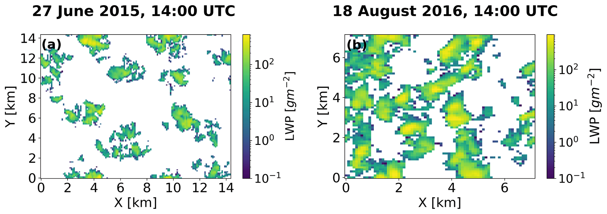
Figure 2Large eddy simulation (LES) of cloud liquid water path (LWP) for 14:00 UTC on 27 June 2015 (a) and 14:00 UTC on 18 August 2016 (b) at the ARM SGP atmospheric observatory. White areas are clear-sky regions where the cloud liquid water path (LWP) is 0.
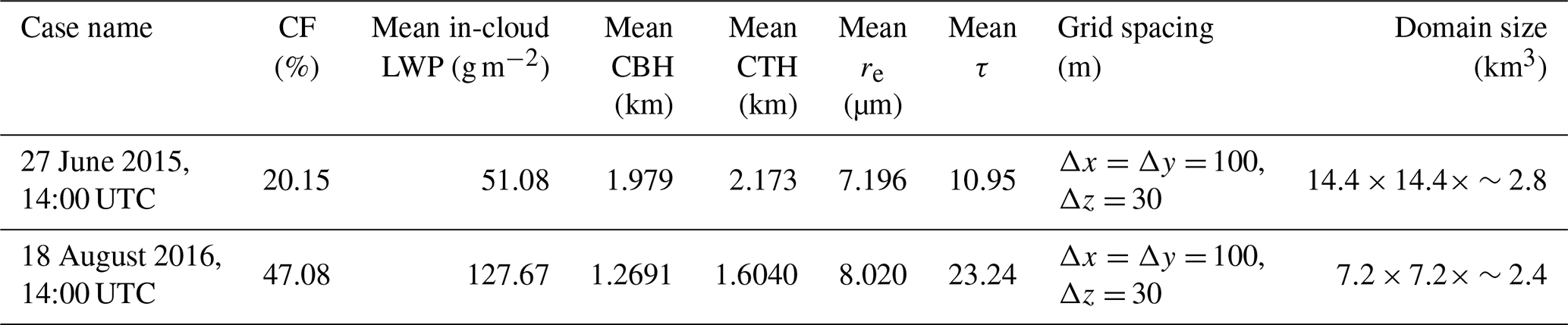
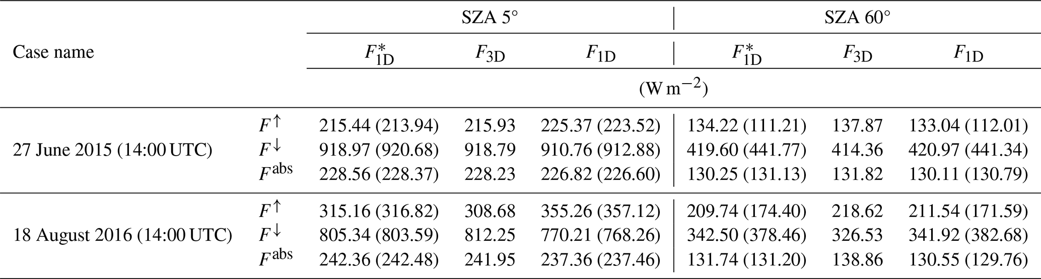
The LASSO LES cloud fields for this study are characterized by broken cloud patterns spatially distributed across the domain as seen in the LWP maps in Fig. 2a and b for the 27 June and 18 August cases, respectively. The 3D distribution of cloud liquid water content (LWC) was obtained from the LASSO cloud field data, and a two-moment bulk microphysics scheme by Morrison and Gettelman (2008) (see their Eq. 5 in Sect. 2) was used to obtain the re associated with the corresponding LWC distribution. It is important to note that for this study, a cloudy column has been defined as a column with LWP > 0 (i.e., clear-sky regions have LWP = 0). The cloud fields have different domain sizes and microphysics distribution, and the cloud cover for the 18 August cloud field (47.08 %) is more than twice that of the 27 June cloud field (20.15 %). Information about the cloud properties and the LES domain is summarized in Table 1.
Table 1Cloud property characteristics for the LES cloud field cases. The mean cloud effective radius (re), mean cloud optical thickness (τ), and in-cloud liquid water path are from the average of the cloudy regions only. The columns from left to right are the case name, cloud fraction, mean in-cloud liquid water path, mean cloud-base height (CBH), mean cloud-top height (CTH), mean re, mean τ, grid spacing, and domain size, respectively.
2.2 Radiative transfer setup
We use the spherical harmonics discrete ordinate method (SHDOM) RT model developed by Evans (1998) to handle both 1D and 3D radiance computations. We have benchmarked the SHDOM simulations against the results from our previous studies (Zhang et al., 2012; Miller et al., 2016). Broadband SW radiative flux computations, both 1D and 3D, were performed with the Intercomparison of 3D Radiation Codes (I3RC) Monte Carlo community model (Pincus and Evans, 2009), and atmospheric gaseous absorption was incorporated via the SW Rapid Radiative Transfer Model (RRTM) correlated k-distribution approach (Mlawer et al., 1997), which consists of 14 bands with a spectral range from 0.2 to 12 µm (this coupled broadband radiative flux solver is hereafter known as the I3RC+CKD model). Rayleigh scattering was included in the flux RT calculations, the background atmospheric profiles are taken to be horizontally homogeneous throughout the domain, and the profiles of atmospheric temperature, pressure, ozone, air density, and water vapor utilized for the RT flux calculations were obtained from the sounding data at the ARM SGP site on 27 June 2015. Several studies (e.g., Gristey et al., 2022) have shown that aerosol embedded in clouds with small aspect ratios (similar to our chosen LASSO LES cloud fields) has a significant influence on the 3D radiative effect. Thus, for simplicity in our study, ambient aerosols are neglected in the RT calculations. The 1D broadband RT flux calculations were performed with the same I3RC+CKD model by dividing the LES domain into individual columns, and RT was calculated on each LES column property separately and independently.
The spectral cloud optical properties were calculated using Mie scattering theory and were averaged over each of the RRTM spectral bands. The phase functions were represented using Legendre coefficients with 35 log-spaced effective radii spanning from 2 to 40 µm. The surface was assumed to be Lambertian with surface spectral albedos obtained from the ARM SGP site (see Fig. 4 in Coddington et al., 2013) applied for wavelength (λ) in the range 0.2 2.5 µm, while surface spectral albedo corresponding to a vegetation-covered surface (Zhuravleva et al., 2009) was utilized for λ> 2.5 µm (see Appendix B for the surface spectral albedo plot used in this study). In the Monte Carlo calculations, 108 and 104 photons were initiated for calculations of the 3D broadband SW flux and the column-independent 1D broadband SW flux, respectively. The radiative transfer calculations were implemented for two solar zenith angles (SZAs), a high-sun case with SZA of 5° and a low-sun case with SZA of 60°. In the broadband flux calculations, the downward flux at the top of the domain (TOD) corresponds to 1363 and 684.1 W m−2 for SZA 5 and 60°, respectively. Throughout this study, we choose a constant 0° solar azimuth angle (SAA) and a constant 0° viewing zenith angle (VZA). Double periodic horizontal boundary conditions were applied for all the RT calculations, and all RT calculations have been conducted at the native LES resolution of 100 m. Current satellite remote sensing instruments have different footprints (e.g., 1 km footprint for MODIS), which can have different 3D effect signatures on the retrievals and impact the derived radiative flux. Therefore, future studies will investigate how 3D effect retrieval errors for different spatial resolutions (coarse and fine) affect the radiative flux estimates.
2.3 Bispectral retrieval method
The bispectral retrieval method introduced in Sect. 1 is solely based on the 1D RT theory to interpret the observed cloud reflectance. It is implemented using a precomputed lookup table (LUT), which consists of 1D reflectance functions for different τ and re combinations at the required solar viewing geometry (an example LUT is shown in Fig. 3). The observed cloud reflectance is then utilized as input to the LUT to simultaneously retrieve the τ and re via a two-dimensional (2D) interpolation between the observed cloud reflectance and the LUT grid. Notably, in the bispectral LUT regions with smaller τ, the retrieval uncertainty increases because the isolines of the LUT τ are less orthogonal and more tightly packed.
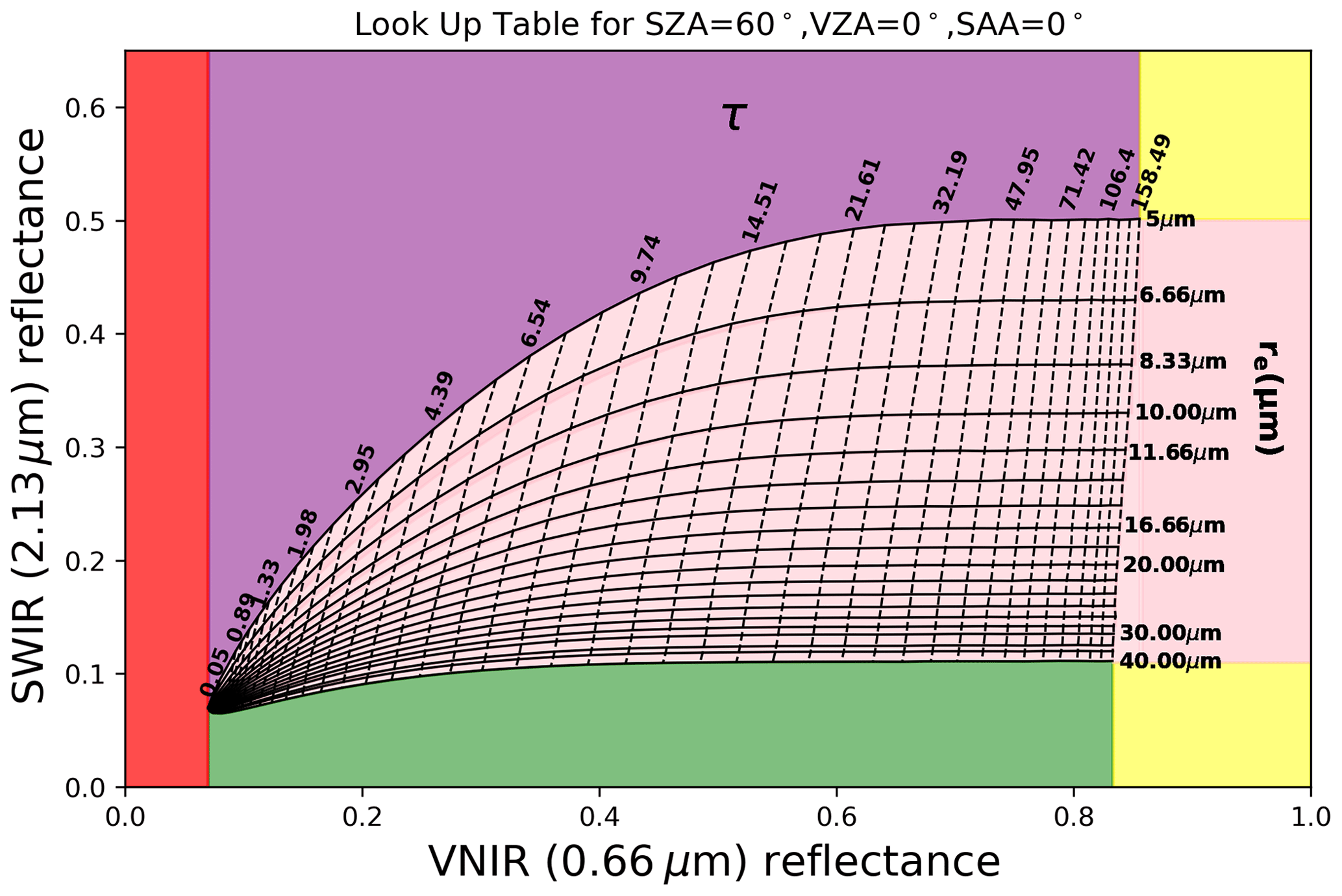
Figure 3An example Nakajima and King (1990) bispectral lookup table (LUT) space. The solid lines are the reflectance function contours for fixed cloud effective radius (re), while the dashed lines are for fixed cloud optical thickness (τ). The surface is Lambertian with a surface albedo of 0.07. The solar zenith angle (SZA) is 60°, the view zenith angle (VZA) is 0°, and the solar azimuth angle (SAA) is 0°.
This nonlinearity in the LUT has high inhomogeneity consequences for cloud retrievals at the pixel level (Zhang et al., 2012, 2016). In this study, the VNIR reflectances were measured at 0.66 µm (identical to the central wavelength of the operational MODIS retrieval algorithm over a vegetated land surface), while the SWIR reflectances were measured at the 2.13 µm wavelength. The LUTs utilized for our bispectral retrievals have 19 effective radii spanning from 5 to 40 µm and 43 log-spaced τ values spanning from 0.05 to 158.48, while a constant effective variance (ve) value of 0.1 is used for consistency with all other RT simulations in this study. The surface albedo at both 0.66 and 2.13 µm wavelengths for the LES radiance simulations and LUT RT calculations was 0.07. This value is consistent with the surface albedo of similar spectral bands in the broadband SW flux computations (see the spectral albedo plot in Appendix B).
2.4 Classification of failed and successful retrievals
One major challenge in cloud property retrievals from satellite remote sensing instruments like MODIS is a so-called “failed retrieval”. A retrieval can be considered failed if there is no re and τ LUT grid combination to interpret the reflectance observation or if there are no realistic cloud microphysics to explain the retrieved cloud property (e.g., a retrieved re> 40 µm). These can be due to several factors, such as the limits of the LUT, cloud overlapping effect, presence of partially cloudy pixels, extreme solar-satellite viewing geometries, strategy used in cloud mask implementation, and the optical characteristics of the underlying surface. Potential causes and rates of occurrence of failed MODIS retrievals for marine liquid-phase clouds have been studied extensively (Cho et al., 2015). In this study, we refer to the MODIS cloud property retrieval algorithm's classification of failed retrievals (Platnick et al., 2016) and the study by Cho et al. (2015) to classify a pixel as a successful or failed retrieval as explained below.
- 1.
For observations with both VNIR and SWIR reflectance observations within the LUT solution space, the nearest interpolated τ and re values are retrieved (pink area bounded by the LUT lines in Fig. 3). If the observed VNIR reflectances exceed the upper limit of LUT τ but within the LUT re solution range (extended pink area in Fig. 3), the nearest LUT re is retrieved and the maximum LUT τ value (τ=158.48) is assigned to the retrieval. These explained categories are classified as “successful retrievals” for this study.
- 2.
In other cases, for observations with VNIR reflectance within the LUT solution space but SWIR reflectance above the LUT solution space (purple area in Fig. 3), the nearest τ values are retrieved but the smallest LUT re value of 5 µm is assigned to the retrievals. This category of retrieval failure is called “re too small” failures. In cases where the VNIR reflectance observations are within the LUT τ solution space but the SWIR reflectances are below the LUT solution space (green area in Fig. 3), the nearest τ values are retrieved but the largest LUT re value of 40 µm is assigned to the retrieval. This category of retrieval failure is called the “re too large” failures. In cases where the observed VNIR reflectance is greater than the largest LUT τ value and the observed SWIR reflectance is smaller than the largest LUT re (i.e., the lower yellow region in Fig. 3), the retrievals are assigned the largest τ value (τ=158.48) and the largest re value (re=40 µm). For observations with VNIR reflectance greater than the largest LUT τ value and the SWIR reflectance greater than the smallest LUT re value (i.e., the upper yellow region in Fig. 3), the retrievals are assigned the largest τ value (τ=158.48) and smallest re value (re=5 µm). Lastly, for observations with VNIR reflectance below the minimum LUT τ (red area in Fig. 3), the re and τ retrievals are assigned fill values (which are represented by τ=0 in our flux calculations). These explained categories are called τ failures. The “re too small”, “re too large”, and τ failure categories are collectively classified as “failed retrievals” for this study.
2.5 Approach for radiative transfer simulation and result comparisons
To address the three SQs for our study (identified in Sect. 1), we performed a total of 14 experiments for each cloud field. The first four experiments were performed with the SHDOM model to study the 3D radiative effects on the observed reflectance and address SQ 1. It involves simulating and comparing R3D with R1D for the high- and low-sun cases. The next four experiments involve comparing cloud properties retrieved from R3D (Box D in Fig. 1) and cloud properties retrieved from R1D (Box B to A in Fig. 1) for both high and low sun to examine the influence of the 3D radiative effects on the retrieved cloud properties and address SQ 2. These experiments were conducted using the 3D- and 1D-RT-based reflectance as inputs to the precomputed LUT described in Sect. 2.3. The last six experiments were conducted with the I3RC+CKD to examine the impact of the 3D radiative effects on the broadband solar radiative flux for both high- and low-sun scenarios in the LES domains and address SQ 3. These experiments involve calculating for each SZA from the retrieved cloud properties using 1D RT as well as computing F3D and F1D from the true cloud fields using 3D and 1D RT, respectively. It is important to note that in the calculations, the retrieved cloud properties (τ∗(R3D) and ) are utilized to calculate the retrieved LWP (using retrieved LWP , where ρ is the density of liquid water; Liou, 1992), which is then reconstructed into cloud effective radius and LWC distribution for each LES column while preserving the vertical structure of the original LES cloud field. 1D RT is then performed using the reconstructed retrieved clouds as inputs to obtain . Note that unless otherwise stated, for this study, the successful and failed retrievals (as described in Sect. 2.4) have been used to represent the total population of cloudy pixels in the cloud property inputs used to calculate . The calculation of F1D is identical to that of F3D except for the absence of the horizontal movement of photons between the LES grid columns. This enables us to determine the impact of neglecting the horizontal movement of photons on the broadband radiative fluxes. On the other hand, in reference to the F3D, computing will not only help us to better understand the implications of neglecting the horizontal transport of photons but will also enable us to measure how biases in the retrieved cloud properties (which are affected by the 3D radiative effects) impact the broadband radiative fluxes.
In order to describe the impact of the 3D radiative effects on the radiance fields, retrieved cloud properties, and broadband radiative flux, we first examine their effects across the LES domain and subsequently quantify their overall impact on the domain by computing the horizontally domain-averaged results to determine the absolute bias, hereafter referred to as “bias” for brevity, defined as , where denotes the domain-averaged result from the 3D RT quantity (e.g., reflectance or flux), and denotes the domain-averaged result from the 1D RT quantity (e.g., reflectance or flux).
To quantify the difference between the CREs computed from the benchmark F3D and the CREs computed from F1D or , we define a domain-scale quantity known as the relative cloud radiative effects (rCRE) bias as
where CRE1D is the CRE calculated from either F1D or in units of W m−2 and CRE3D is the CRE calculated from F3D in units of W m−2. According to this definition, a rCRE bias of 0 % would indicate that there is no bias between the CRE computed from F1D or and the CRE computed from F3D. This implies that the CRE computed from F1D or is equivalent to the CRE computed from F3D. A positive rCRE bias greater than 0 % would quantify the percentage by which the CRE computed from F1D or is lesser than the CRE computed from F3D and thus indicate that the 1D calculations (F1D, ) underestimate the CRE relative to F3D. Also, a negative rCRE bias less than 0 % would quantify the percentage by which the CRE computed from F1D or exceeds the CRE computed from F3D and imply that the calculations from F1D or overestimate the CRE relative to F3D.
3.1 Investigating the 3D radiative effects on simulated reflectance
Focusing first on SQ 1, we compare R1D and R3D to assess the impact of the 3D radiative effects on the reflectance radiation field, i.e., Box B vs. Box C in the framework of Fig. 1. Specifically, we will investigate the reflectance bias, , at the two λ values (0.66 and 2.13 µm) required for our bispectral retrieval for both low-sun (SZA 60°) and high-sun (SZA 5°) cases. To describe the 3D radiative effects on the observed reflectance, classifications are made based on the increase in the brightness of a pixel in the LES domain. A pixel in the LES domain is considered “brightened” (“darkened”) if its 3D-RT-based reflectance is higher (lower) than its 1D counterpart.
Maps of δR at λ=0.66 µm (δRλ=0.66 µm) for the two cloud fields when the sun is high and low are shown in Fig. 4. In the low-sun case, the deviation of the 1D-RT-based simulated reflectance from the 3D-RT-based simulated reflectance leads to δR with a distinct pattern of brightening and darkening observed in some pixels across the LES domain. A closer examination of δRλ=0.66 µm within cloudy regions in the low-sun case for the two cloud fields (Fig. 4b, c) reveals a consistent pattern; the brightened pixels, where δRλ=0.66 µm is positive, are predominantly observed in sunlit regions that directly face the sun located on the left (e.g., at X=3.5 km, Y=14 km in Fig. 4b). On the other hand, darkened pixels, where δRλ=0.66 µm is negative, are observed on the opposite side of the cloud layer (e.g., at X=5 km, Y=14 km in Fig. 4b). These findings are consistent with previous 3D radiative effect studies for oblique solar geometry (e.g., Várnai and Davies, 1999; Várnai, 2000; Marshak et al., 2006). The observed opposing effects of brightening and darkening in the low-sun-angle case depend not only on the orientation of the cloud towards or away from the sun; other factors like cloud–cloud interactions, cloud geometry and aspect ratio, spatial distribution of the cloud in the domain, and the horizontal transport of photons also contribute to these behaviors (Várnai and Marshak, 2001, 2002; Marshak and Davis, 2005; Marshak et al., 2006; Zhang et al., 2012).
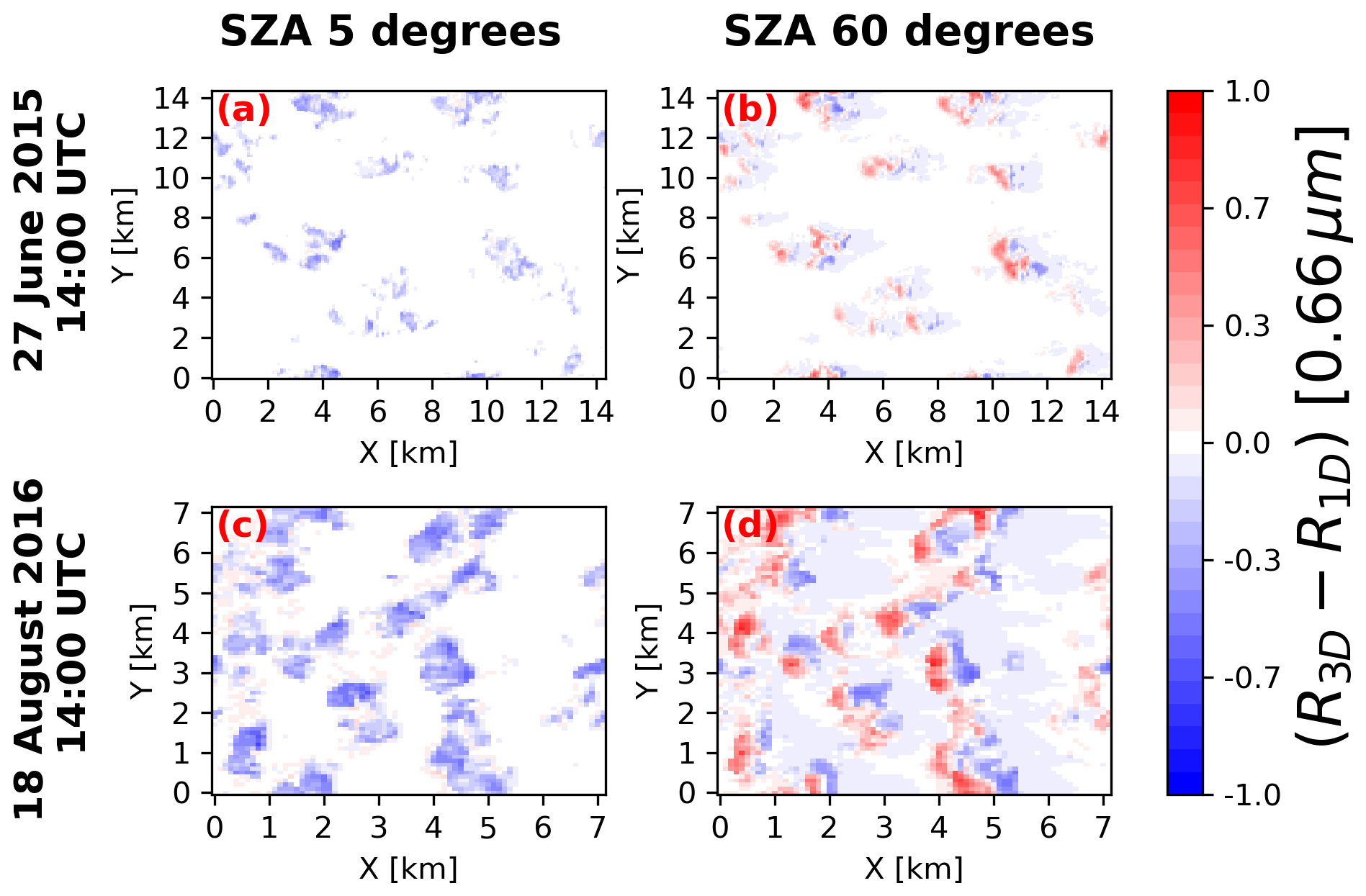
Figure 4Maps of the reflectance bias () for wavelength 0.66 µm at solar zenith angle (SZA) 5° (a, c) for the 27 June and 18 August cases, respectively, and SZA 60° (b, d) for the 27 June and 18 August cases, respectively. The direction of view is at nadir. For SZA 5°, the sun is almost perpendicular to the domain but slightly tilted to the left. For SZA 60° the sun is on the left of the domain.
In the case of the high sun, the sun is almost perpendicular (at SZA 5°), and its radiation interaction with clouds under 3D RT is different from that of the low-sun case. In 3D RT at high sun, the original direction of photons is downwards (due to the sun's small angle of inclination to the vertical), and on striking a cloud, some photons are scattered and some leak from optically thick to optically thin cloudy regions and even out of cloud sides (O'Hirok and Gauiter, 1998) down to the surface where they are absorbed. This is because for photons with a low number of scattering trajectories and high sun, photons leaking out of cloud sides are statistically more likely to continue moving downwards towards the surface where they are absorbed. This leaking of photons to surrounding clouds and the surface results in net photon loss in the thick cloud regions, which explains the darkening of the thick clouds and brightening of the surrounding thin clouds compared to 1D RT results. Hence, δRλ=0.66 µm is mainly negative across the LES domain for the high sun (Fig. 4a, c). The darkening characteristics are more pronounced in the 18 August case because it consists of a larger distribution of thicker clouds compared to the 27 June cloud field; a large number of photons leaking from optically thicker clouds results in a more significant reduction in the reflectance values and more prominent darkening effect than photons leaking from optically thinner clouds. Similar reflectance characteristics are observed for the 2.13 µm band (not shown).
To examine the statistical characteristics of δR in the LES domain, the probability density function (PDF) of δR for “cloudy only” pixels is analyzed to investigate the 3D radiative effects on the observed cloud reflectance. Subsequently, we compared this PDF to δR for both “cloudy and clear-sky” pixels (i.e., the whole LES domain) to highlight the effects of cloud presence on the overall reflectance bias within the LES domain.
The PDFs of δR for cloudy only pixels in the low-sun case (broken black and gray lines in Fig. 5a, b) are characterized by a positive and negative distribution in both the VNIR and SWIR bands (corroborating the brightening and darkening effects in Fig. 4b, d). The overall positive δR observed in the VNIR and SWIR bands (domain mean δR of 0.0351 (0.0292) for the VNIR (SWIR) band in the 27 June case and 0.0379 for the VNIR band in the 18 August case) indicates that the brightening effects are predominant when only cloudy pixels are considered. Meanwhile, δR is −0.0233 for the SWIR band in the 18 August case. This negative δR is due to a high net loss of photons in 3D RT reflectance (more photons leak from clouds to the surface where they are absorbed than those reflected from clouds) compared to the 1D RT results. On the other hand, the PDFs of δR for the cloudy and clear-sky pixels (broken black and gray lines in Fig. 5c, d) are almost similar to that of the cloudy only but show a shift of the distribution leftwards, almost centered around zero. This is expected because clear-sky regions not in the vicinity of any clouds exhibit negligible 3D radiative effects, which causes the distribution to shift closer to zero, since the cloud fraction for both cloud cases is less than 50 %. The horizontal movement of photons from cloudy to surrounding clear-sky regions increase the 3D reflectance of clear-sky areas around the sunlit cloudy regions but the strong darkening effects on the clear-sky regions located opposite the sunlit direction dominate the clear-sky only areas and result in a negative mean bias when the reflectance of clear-sky only pixels is examined. Interestingly, the mean δR for the cloudy and clear-sky pixels is of the same sign as the cloudy only values, which indicates that the cloudy pixels have a significant effect on the domain-scale statistics.
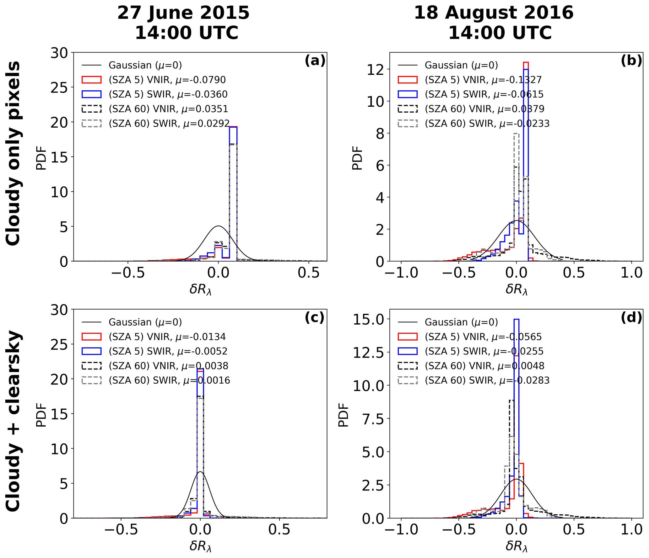
Figure 5PDF (probability density function) of reflectance bias (δR) for cloudy only pixels for the 27 June case (a) and 18 August case (b). PDF of reflectance bias for cloudy and clear-sky pixels for the 27 June case (c) and 18 August case (d). μ is the domain mean reflectance bias. A Gaussian distribution (solid black curve) with a standard deviation for the 0.66 µm band at SZA 5° and centered around zero is shown in all panels.
The PDFs of δR in the case of the high sun for cloudy only pixels show a larger distribution of pixels with positive δR in both the VNIR and SWIR band accompanied by longer tails to the left (solid red and blue lines in Fig. 5a, b). However, the δR values for both cloud cases are negative in the VNIR and SWIR bands. These observations suggest that large amounts of radiation and/or a large number of photons leak from a small number of thick cloud pixels to a larger number of thin clouds. This phenomenon therefore increases the number of thin clouds with positive reflectance bias, although this is of very small magnitude when compared to the negative biases.
Similar to the low-sun case, the PDF of δR when both cloudy and clear-sky pixels for the high-sun case are considered (solid red and blue lines in Fig. 5c, d) shows a significant distribution of values close to zero. Due to the leaking of photons from thick clouds to thin clouds and clear-sky regions surrounding the clouds, there is an increase in the 3D reflectance of clear-sky regions. Additionally, when the sun is high at SZA of 5°, there are very minimal shadows cast on the clear-sky regions. These two highlighted reasons result in a positive δR for the clear-sky-only region. Thus, the negative value of δR for cloudy and clear sky (same sign as the cloudy only) indicates that the domain-scale reflectance bias is dominated mainly by the cloudy only pixels and they play a significant role in the domain-scale statistics.
3.2 Investigating the 3D radiative effects on cloud retrievals
Focusing on SQ 2 in this section, we investigate how δR, as discussed in the previous section, affects re and τ retrievals (i.e., Box A vs. Box D in the framework of Fig. 1). We utilize R1D as inputs for the LUT (explained in Sect. 2.3) to retrieve the 1D-RT-based cloud droplet effective radius and cloud optical thickness (τ∗(R1D)) Additionally, we use R3D as inputs for the LUT to retrieve the 3D-RT-based cloud droplet effective radius and cloud optical thickness (τ∗(R3D)).
Before discussing analysis of the 3D- and 1D-RT-based retrieval comparison, we first check the accuracy of our retrievals by comparing the original LES cloud properties with our 1D-RT-based retrievals (i.e., comparing retrievals from 1D radiance in Box C with cloud properties in Box A in Fig. 1). For this purpose, the τ from the original LES (τtrue) is the vertical integration of the visible (0.66 µm) extinction coefficient of each column from cloud base to cloud top. For the LES re, we the follow Zhang et al. (2017) analytical vertical weighting function (see their Eq. 4) to get the vertically weighted cloud droplet effective radius () where μo=0.5, μ=1, and the vertically weighting function parameter (b) associated with the 2.13 µm band was set to 2 to allow for a deeper penetration depth and for better correlation between the ) and bispectral retrievals.
Figure 6 shows the comparison between the (2.13 µm) and the ) as well as τtrue with the τ∗(R1D) for the two cloud fields at SZA = 60° and VZA = 0°. For this comparison, the mean τ and re biases are and .
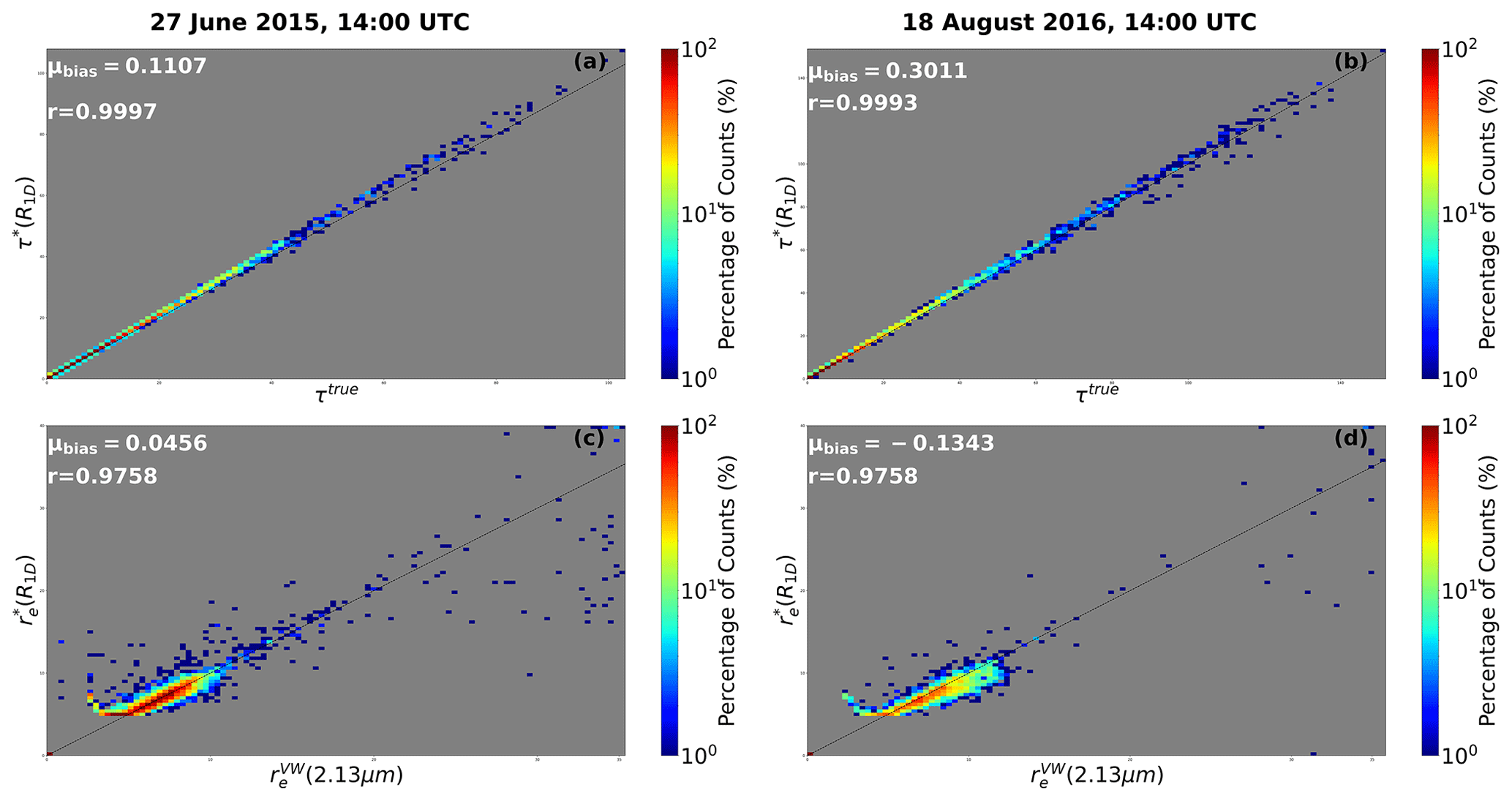
Figure 6Joint histogram of bispectral retrieved τ based on 1D-RT-simulated reflectance τ∗(R1D) vs. vertically integrated τ(τtrue) for the 27 June case and (a) 18 August case (b). Joint histogram of bispectral retrieved re based on 1D-RT-simulated reflectance ( vs. vertically weighted effective radius ( in (c) and (d). The μbias is calculated as 〈retrieved cloud properties−reference cloud property〉.
For the two cloud fields considered in this study, the τ∗(R1D) is highly correlated with the τtrue as seen in the joint histogram plots (Fig. 6a and b) with a correlation coefficient (r) of 0.9997 for the 27 June case and r of 0.9993 for the 18 August case, although both have a slight positive mean bias (μτ bias= 0.1107 and 0.3011 for the 27 June and 18 August cases, respectively). Also, the comparisons of the ) with the ) in Fig. 6c and d show good correlation (r>0.96) for both cloud cases and slightly positive mean biases for the 27 June case as well as a negative mean bias for the 18 August case. Certain extreme outlier bias is observed in the re comparisons; these outliers are attributed to thin clouds and have been studied by Miller et al. (2018). Several studies (e.g., Miller et al., 2016, 2018; Zhang et al., 2012) have investigated the accuracy of 1D bispectral retrievals compared to vertically weighted retrievals as well as the impact of cloud vertical profile on bispectral retrievals. Since we have good agreement between retrievals from the 1D-RT-based reflectance and the original LES cloud field properties, this study will use the ) and τ∗(R1D) as the reference cloud properties and directly compare them with the ) and τ∗(R3D) to investigate the impacts of 3D radiative effects on the retrievals.
In the high-sun case retrievals, ) is overestimated and τ∗(R3D) is underestimated compared to their 1D counterpart. This is because photons leaking from optically thick regions to optically thin cloudy regions and out of cloud sides down to the surface where they are absorbed results in a net photon loss, which makes the 3D radiance field appear darker than its 1D counterpart (explained in Sect. 3.1). Consequently, for retrievals, darkening shifts the reflectance observation on the LUT space leftwards and downwards to regions where the LUT re grid isolines represent larger droplet sizes and the LUT τ isolines represents thinner clouds. For the low-sun case, ) is underestimated and τ∗(R3D) overestimated in brightened optically thick cloudy pixels (facing the sun), and ) is overestimated and τ∗(R3D) underestimated in darkened pixels on its opposite cloud side. Larger ) and smaller τ∗(R3D) compared to τ∗(R1D) and τ∗(R1D) in brightened pixels occur since brightening phenomena in the LUT space shift the observed reflectance upwards and rightwards where the LUT re grid isolines represent smaller droplet sizes and the LUT τ isolines represent thicker clouds. τ and re retrieval biases in satellite observations have been well documented in numerous studies (e.g., Várnai and Marshak, 2002; Zhang and Platnick, 2011; Zhang et al., 2012), and commonly, overestimation of τ∗(R3D) is coupled with the underestimation of ) and vice versa.
Table 2 shows the frequency of failed and successful retrievals from R3D for the two cloud fields considered in this study. It is observed that the number of failed retrievals is small for the SZA 5° case (< 13 %), while the retrieval failures are larger for the SZA 60° case (> 40 %) for both cloud fields under consideration. The larger retrieval failures for the low-sun case are mostly attributed to multiple scattering in the 3D RT due to increased path length (since the original direction of travel of the photons from the sun is oblique), which increases radiation–cloud interaction and reflectance. Although this leads mostly to τ failures, the other re type failures can arise from very darkened pixels (from photon leaking or cloud shadow), which shifts observation outside the LUT lower range (for re too large), or brightened pixels from less absorbing clouds, which shifts the observations beyond the upper range of the LUT (for re too small) depending on the scenario.
Table 2Statistics of successful and failed retrievals from the 3D-RT-based radiance for the 27 June and 18 August cloud fields at solar zenith angle (SZA) 5 and 60°. The columns from left to right are the case name (identified by date and time), solar zenith angle (SZA), number of pixels with successful retrievals only, pixels with failed retrievals, and total number of successful and failed retrievals.
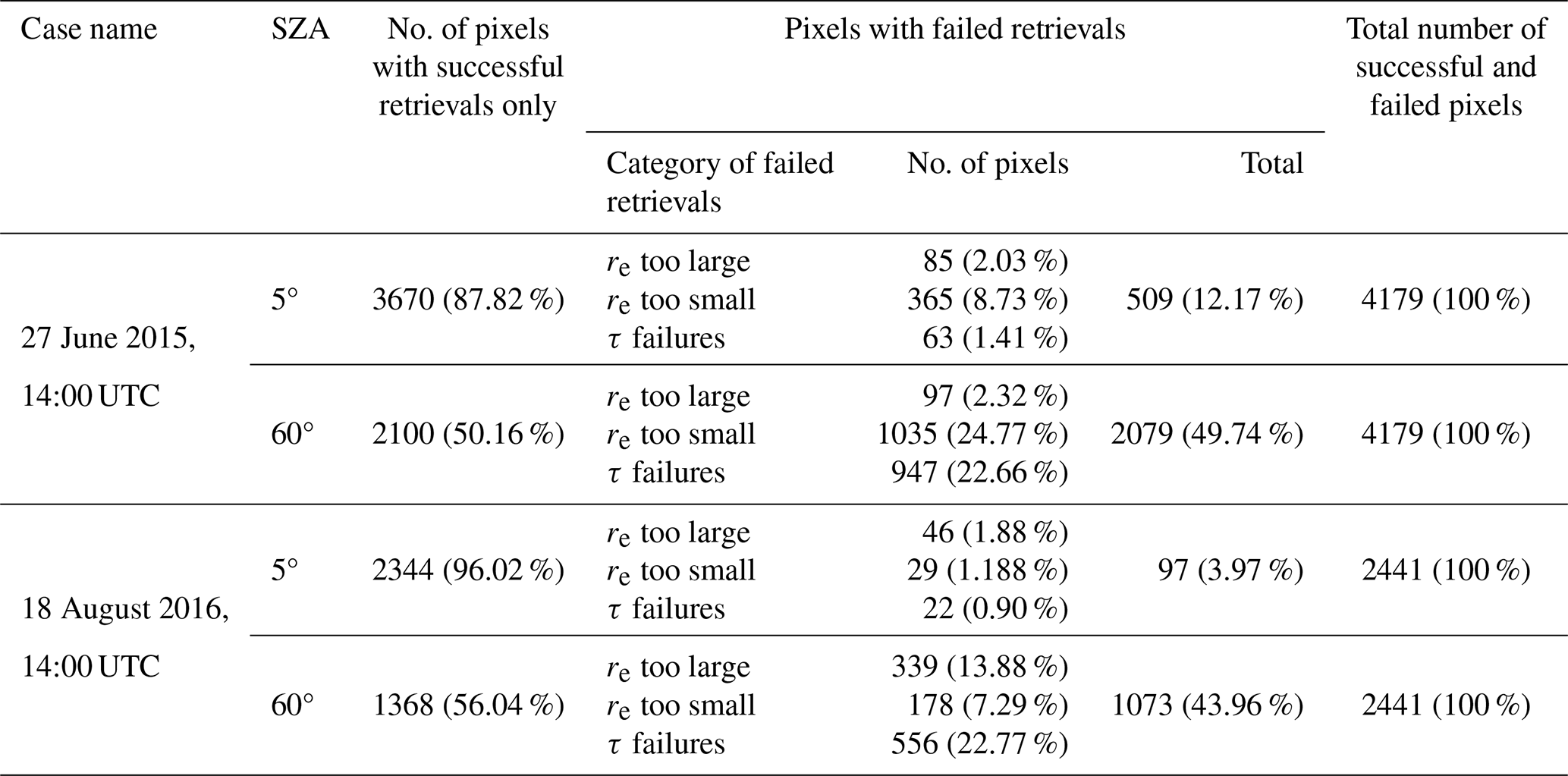
Values in parentheses are percentage counts (percentage of counts equals the number of affected pixels divided by the total number of pixels).
3.3 Investigating the 3D radiative effects on the broadband radiative flux
Investigating the 3D radiative effects on the broadband radiative flux: using a combination of the successful and failed retrievals as the input cloud property
Focusing on SQ 3 in this section, we will compare F3D and to investigate the impact of cloud retrieval biases due to the 3D radiative effects on the broadband SW radiative flux. We will also compare F3D and to study the impact of neglecting horizontal photon transport on the broadband SW flux results. Additionally, we compare δF1 (i.e., ) with δF2 (i.e., F3D−F1D) to determine errors in radiative flux estimates and evaluate the CRE.
It is important to note here that both the successful and the failed retrievals as described in Sect. 2.4 are included in the RT simulations in the control simulations presented in this section. The motivation for including the failed retrievals is to preserve the impacts of this significant fraction of pixels on the domain-averaged fluxes and CRE simulations, even though the retrieval of τ and re based on the bispectral method fails for them. In addition to the controlled simulations, we have also conducted sensitivity studies, where we exclude the failed retrievals in the analysis. The results are shown and discussed in the Appendix A.
Maps of the simulated SW broadband radiative quantities (reflected flux at the TOD (F↑), transmitted flux at the surface (F↓), and column absorbed flux (Fabs)) for the 27 June case at the high and low sun angles are presented in Figs. 7 and 8, respectively. These figures reveal several interesting and important points. First, it is interesting to note that the reflected flux in Fig. 7d seems blurry in comparison with 1D results in Fig. 7a and g. The same is also seen comparing Fig. 8d with Fig. 8a and g. This is because in 1D RT, simulation of the upwelling hemispheric flux at a given point at the TOD is determined only by the cloud and surface properties in the column beneath such a point. In contrast, in 3D RT simulation, it depends on the cloud and surface properties of both the corresponding column and a large extent of the surrounding columns as a result of a simple parallax effect. Therefore, the contrast between two adjacent columns in the 1D simulation, for example a cloudy column and an adjacent clear-sky column next to it, is quite large, whereas the contrast for the same two columns in 3D simulation is much smaller because the two have a significant overlap in terms of the areas that have influences on their flux. Because of this fundamental difference between 1D and 3D simulations, a pixel-to-pixel comparison of the upwelling flux is not appropriate. Instead, we compare the domain-averaged statistics.
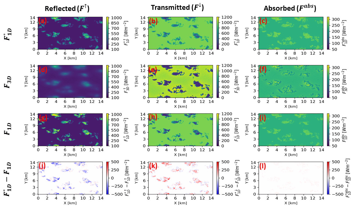
Figure 7Simulated shortwave broadband reflected flux at the top of the domain (F↑), transmitted flux at the surface (F↓), and column absorbed flux (Fabs) derived from the retrieved cloud properties using 1D RT and (a–c), derived from the true cloud properties using 3D RT and F3D (d–f), derived from the true cloud properties using 1D RT and F1D (g–i), and the difference between and F1D (j–l) for a solar zenith angle of 5° and a view zenith angle of 0°. The sun is high and slightly on the left-hand side of the domain. The solar irradiance at the top of the domain scales with the cosine of the solar zenith angle.
Before we delve into that, we first aim to unravel how cloud property retrieval errors affect 1D RT flux solutions. For this purpose, we compare the F↑ component of (denoted by ) with the F↑ component of F1D (denoted by ). The same comparison is done between the F↓ component of (denoted by ) and its counterpart from the F1D (denoted by ). The has visible signatures of the input cloud property retrievals. For instance, in the high-sun case, smaller reflected flux values (recall the underestimated τ dominates retrievals from high sun radiance) dominate (Fig. 7a) compared to (Fig. 7g). The underestimation of compared to is evident in Fig. 7j. This difference is also well captured in the domain-averaged values, which will be discussed later in this section. In the low-sun case, comparison between and corresponding reveals that in , the overestimated retrieved τ areas characterized by thicker clouds (i.e., retrieved from brightened pixels) provide larger reflected flux values and the underestimated retrieved τ areas characterized by thinner clouds (i.e., retrieved from darkened pixels) have smaller reflected flux values than their counterpart (Fig. 8j). Their overall effect on the domain reflected flux values depends on how the opposite 3D radiative effects (cloud side brightening and darkening) mitigate each other.
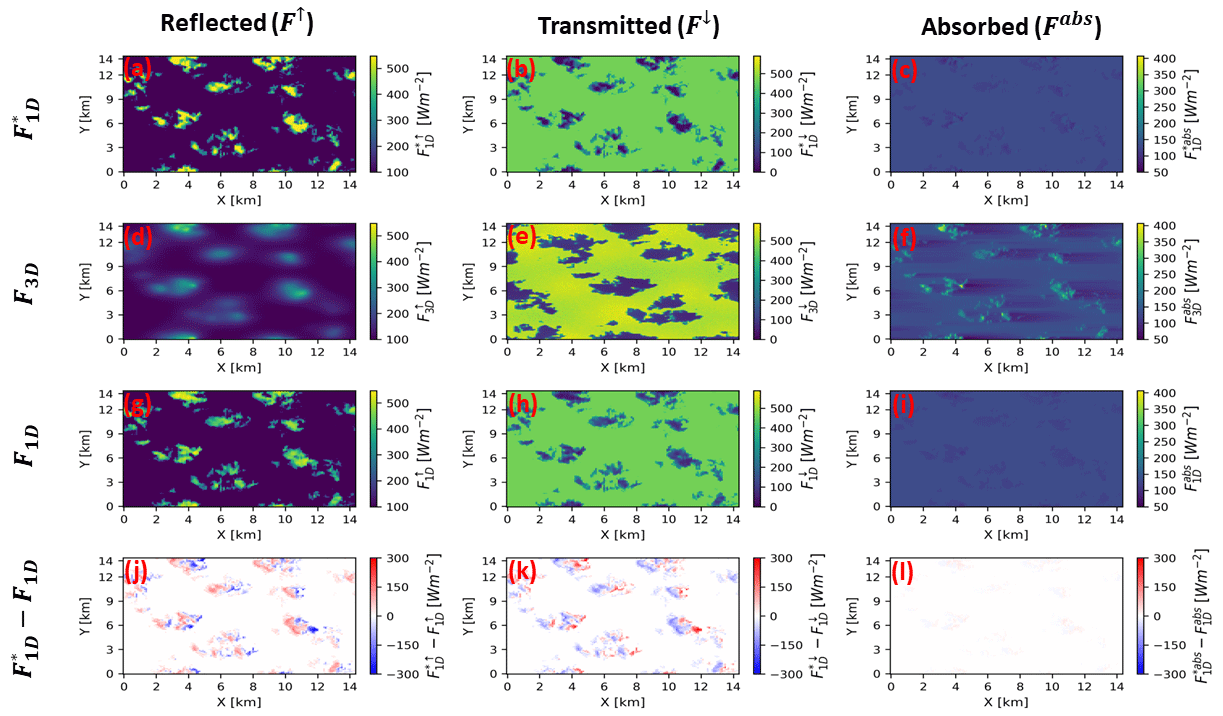
Figure 8Simulated shortwave broadband reflected flux at the top of the domain (F↑), transmitted flux at the surface (F↓), and column absorbed flux (Fabs) derived from the retrieved cloud properties using 1D RT and (a–c), derived from the true cloud properties using 3D RT and F3D (d–f), derived from the true cloud properties using 1D RT and F1D (g–i), and the difference between and F1D (j–l) for a solar zenith angle of 60° and view zenith angle of 0°. The sun is on the left-hand side of the domain. The solar irradiance at the top of the domain scales with the cosine of the solar zenith angle.
An examination of and for the high-sun case reveals that beneath clouds is larger compared to , while they have same values in clear-sky regions (Fig. 7k) This is expected since is less than . Thus, the amount of at the surface beneath the cloud increases. For the low-sun case, and beneath the clouds have higher values where the TOD reflected flux is low and lower values where the TOD reflected flux is high (Fig. 8k).
The radiative quantities across the LES domain have different characteristics in F3D stemming from the horizontal transport of photons across pixels. For the high-sun case, aside from the blurriness of the F↑ component of F3D (denoted by ) which was previously explained, an examination of the F↓ component of F3D (denoted by ) in Fig. 7e shows a slight tilt of the cloud shadows according to the angle of projection of the sun (located at SZA 5° to the left). It also reveals enhanced values around cloud edges. Such is not the case in (Fig. 7h) due to 1D RT setup where each cloudy column is considered independent. These observations are consistent with findings made by Gristey et al. (2020) for similar shallow cumulus cloud fields. Gristey et al. (2020) showed that enhanced around cloud edges is primarily caused by the diffused component of the transmitted flux, which is scattered by clouds towards clear-sky regions beyond cloud shadows. In for the low sun (Fig. 8e), due to 3D RT and the more oblique solar angle (SZA 60°), there is an increase in the total effective cloud cover (Di Giuseppe and Tompkins, 2003; Tompkins and Di Giuseppe, 2007), as well as an increase in the size of the cloud shadow, which reduces the transmitted flux at the surface (e.g., around X=7, Y=6 km) in Fig. 8e. Just as in the case of the high sun, these features are absent in the low-sun 1D RT runs ( and ). An analysis of the domain-averaged statistics will help shed more light on the differences between the 3D RT and 1D RT radiative flux results on the domain scale.
Table 3Statistics of successful and failed retrievals from the 3D-RT-based radiance for the 27 June and 18 August cloud fields at solar zenith angle (SZA) 5 and 60°. The columns from left to right are the case name (identified by date and time), solar zenith angle (SZA), number of pixels with successful retrievals only, pixels with failed retrievals, and total number of successful and failed retrievals.
Note: values before the parentheses are calculated from the combination of failed and successful retrievals representing the total cloudy population, while values in parentheses are calculated from successful retrievals only representing the total cloudy population. Clear-sky pixel values have been included in all calculations.
The domain-averaged broadband F↑, F↓, and Fabs components of , F1D, and F3D for the 27 June and 18 August cases at SZA 5 and SZA 60° are reported in Table 3. As previously explained, the predominant photon leaking associated with high-sun 3D RT and the ensuing underestimation of the retrieved τ, which dominate the cloud property retrievals from high-sun 3D-simulated reflectance, increase the number of retrieved optically thinner clouds (relative to the original LES τ used in F1D calculations) utilized as inputs for the calculations. This leads to the underestimation of the domain-averaged compared to ; In the 27 June case, the domain-averaged (215.44 W m−2) is underestimated compared to the corresponding value (225.37 W m−2) by about 9.93 W m−2, while in the 18 August case, the domain-averaged (315.16 W m−2) is underestimated compared to the corresponding value (355.26 W m−2) by 40.1 W m−2. The larger value of the underestimated domain-averaged in the 18 August case stems from its larger cloud fraction and τ bias. The transmitted flux at the surface below clouds is dependent on the amount of flux reflected towards the TOD; lower reflected flux values indicate that less radiation is reflected from the clouds, which allows a greater amount of radiative flux to be transmitted to the surface beneath the clouds. This reason, coupled with the overestimation of the transmitted flux at the surface due to missed thin clouds in our bispectral retrievals (red regions in Fig. 3, retrieved τ=0 for VNIR reflectance less than the smallest LUT τ value), explains why for the high-sun case the domain-averaged values are higher compared to values, resulting in differences of 8.21 and 35.13 W m−2 for the 27 June and 18 August cases, respectively, although for the high sun angle the contribution of the missed thin clouds to the overestimation of beneath clouds in our case study is small (constituting about 0.23 % and 0.34 % of the domain-averaged surface transmitted flux for the 27 June and 18 August high cases, respectively).
Comparing results from the three sets of experiments in Table 3 reveals that for the high-sun case, the results clearly agree better with the benchmark F3D than the F1D results. In the 27 June case, δF1 values for the domain-averaged F↑, F↓, and Fabs are 0.49, −0.18, and −0.33 W m−2, respectively, which are significantly smaller in magnitude than those for δF2 (−9.44, 8.03, and 1.41 W m−2, respectively). Similarly, for the 18 August case, δF1 for the domain–averaged F↑, F↓, and Fabs are −6.48, 6.81, and −0.41 W m−2, respectively, compared to corresponding biases of −46.58, 42.04, and 4.59 W m−2 for δF2. These results suggest that gives an overall better radiative energy estimate than F1D for the high-SZA case. In the low-sun case, the and F1D are very close to each other and there is no clear winner when compared to the benchmark 3D RT results. In the 27 June case, the agrees slightly better with 3D results than the F1D, but the opposite is true in the 18 August case. This result seems to suggest that although in the low-sun case the brightening and darkening effects can lead to large retrieval biases, they tend to cancel each other out in the flux computations. Interestingly, both 1D results tend to underestimate F↑ and overestimate F↓. This is probably because the brightening effect is dominant in the 3D RT, leading to some extremely bright pixels. But they are not captured in the 1D RT computations, even in the using the upper limit of τ=158.48 in the flux computation. Thus, the reflected flux quickly reaches the asymptotic value when τ is large, and therefore simply using larger τ value in 1D RT cannot simulate the extreme brightness of clouds due the brightening effect in 3D RT. Results for δF2 computed from the transmitted flux at the surface for both cloud cases (27 June and 18 August) are positive when the sun is high (8.03 and 42.04 W m−2) and negative for the low sun angle (−6.61 and −15.39 W m−2), consistent with Gristey el al. (2020) for surface irradiance showing positive domain mean δF2 in the afternoon (high sun) and negative domain mean δF2 towards the end of the day (low sun).
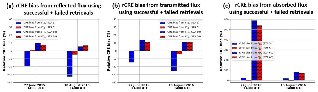
Figure 9Relative cloud radiative effect (rCRE) bias computed from the successful + failed retrievals for the (a) reflected flux at the top of the domain, (b) surface transmitted, and (c) absorbed for the two cloud fields.
Because both cloud cases have a cloud fraction lower than 50 %, the domain-averaged statistics include a large fraction of clear-sky pixels. Now we focus our scope on cloudy pixels and investigate the differences in CRE. The rCRE bias provides a quantitative estimate of how these biases affect the CRE. For the two cloud cases considered in this study, plots of rCRE bias computed from the F↑, F↓, and Fabs at SZA 5 and 60° for and F1D relative to F3D are presented in Fig. 9. In the 27 June case, the rCRE bias of 0.97 % computed from the high-sun result indicates a negligible deviation (less than 1 %) from the benchmark CRE, while the rCRE bias of −19 % computed from the high-sun result shows that the bias is quite substantial. Similarly, for the 18 August case, the rCRE bias computed from the high-sun result is less than 5 %. On the other hand, the rCRE bias of −32.48 % computed from the high-sun result shows that the bias is quite large. Similar results are obtained for rCRE bias computed from F↓. In the 27 June case, the rCRE bias computed from the is 0.33 % (Fig. 9b, second bar on the left), which shows minimal bias less than 1 %, while the rCRE computed from the is −14.5 % (Fig. 9b, first bar on the left). Similarly, for the 18 August case, the rCRE bias computed from the is −4.12 % (Fig. 9b, second bar on the right), while the rCRE bias computed from the is −25.10 % (Fig. 9b, first bar on the right).
When the absorbed flux is taken into consideration, for the 27 June high-sun case, the rCRE bias computed from the absorbed component of () is −6.05 % (Fig. 9c, second bar on the left), which is less bias compared to the 25.64 % rCRE bias computed from the absorbed component of F1D () (Fig. 9c, first bar on the left). Similarly, for the 18 August case, the rCRE bias computed from is −1.73 % (Fig. 9c, second bar on the right), while the rCRE bias computed from is 19.09 % (Fig. 9c, first bar on the right). For the low-sun case, the rCRE biases computed from and F1D are comparable, which is consistent with the domain-averaged statistics in Table 3. Evidently, both and F1D overestimate the CRE at TOD and surface, which means an underestimation of cloud reflection and overestimation of transmission. This is consistent with the results in Table 3.
Overall, the above analysis indicates that the provides results that are better than (in the high-sun case) or at least comparable to (in the low-sun case) F1D for both domain-averaged flux statistics and CRE when compared to the benchmark F3D results. With these results we can conclude that the CRE calculated with 1D RT using retrieved cloud properties, which are biased due to the 3D effects, is found to be comparable to or better than the CRE calculated with 1D RT using the true cloud properties.
It is well known that bispectral cloud property retrievals based on the 1D RT have significant errors due to the 3D radiative effects. In this study, we investigate whether the biased retrievals can still be used to estimate the broadband flux and CRE. To address this question, we selected two cloud fields from the LASSO activity, one on 27 June 2015 and another on 18 August 2016, to serve as case studies for our research. The LES cloud fields have different microphysics with different CBH and CTH, and the value of the cloud fraction for the 18 August 2016 cloud field (47.08 %) is more than twice that of the 27 June 2015 (20.15 %) cloud field. Radiance simulations, bispectral retrievals, and broadband SW flux radiative transfer simulations were performed using these cloud fields at two SZAs, a high-sun case (SZA = 5°) and a low-sun case (SZA = 60°), and the results were analyzed. The flux computations were carried out in three sets. The reference broadband SW flux calculations were performed using the cloud properties from the original LES cloud field under 3D RT (F3D). We also computed similar RT broadband SW flux calculations with the same cloud properties from the original LES cloud field except that the RT calculations were computed using 1D RT (F1D). Additionally, we computed the last set of broadband SW flux calculations using 1D RT and bispectrally retrieved cloud properties as inputs ().
The high sun radiance results for the two cloud fields show that in the 3D RT high-sun case, the photons leaking from optically thick cloudy regions to optically thin cloudy regions and the surface dominate the LES reflectance field. This results in overestimated re and underestimated τ dominating the cloud property retrievals. Results from the low-sun case, for the two cloud fields considered, show that in comparison to the 1D RT radiance fields, brightening and darkening effects both occur in the 3D-RT-simulated radiance observation. Therefore, retrievals from the low-sun 3D radiance observations are characterized mainly by both overestimation of τ and underestimation of re in brightened pixels and underestimation of τ and overestimation of re in darkened pixels. The cumulative effects of these brightening and darkening or photon leaking effects and their impacts on the retrieved cloud properties dictate their impact on the broadband radiative flux.
The results from the broadband SW radiative flux computation showed that, although the bispectrally retrieved cloud properties are often biased due to the 3D radiative transfer effects, for high-sun cases, calculations of the CRE from these values agree well with the benchmark values (which is the F3D in our case) with agreement within 7 % for rCRE bias calculations from the reflected, transmitted, and absorbed fluxes in the high-sun cases. Conversely, the rCRE bias computed from the F1D quantities could reach about 33 %. Thus, for high-sun situations, the provides consistently better estimates of the CRE than the F1D. For the low-sun case, the two 1D RT experiments provide comparable results, both underestimating cloud reflection and overestimating transmission, and there is not a clear winner when compared to the 3D RT benchmark.
The influence of the failed retrievals on the CRE was also investigated (see details in Appendix A), with results indicating that for the high-sun case, the impact of the failed retrievals on the radiative flux quantities is negligible, with less than 6 % changes observed in the rCRE bias computed from the domain-averaged TOD reflected, surface transmitted, and absorbed and F1D results. Such is not the case for the low-sun case where the failed retrievals have a very huge impact on the radiative flux quantities. Excluding the failed retrievals from the domain-averaged reflected, transmitted, and absorbed and F1D low-sun case analysis could increase the rCRE bias by as much as a factor of 6 compared to values which included the failed retrievals in the analysis. Whether or not to always use the failed retrievals in the radiative flux and CRE estimation is still an important question, especially how best to filter out the failed retrievals from cloud properties retrieved from instruments that rely on the bispectral method (e.g., in MODIS cloud products) for use in radiative flux estimation. We observed here that filtering out all failed retrievals, especially from the low sun angle, can greatly impact the radiative flux estimates. Thus, efforts should be made to study which category of failed retrievals is most relevant for use in CRE estimation.
In conclusion, despite the potential biases due to the 3D radiative effects, the retrieved cloud properties based on 1D RT from the bispectral method still provide CRE estimates that are comparable to or better than CRE calculated from the true cloud properties using 1D RT. Some future questions that warrant answers involve how the 3D radiative effects affect the broadband fluxes for different cloud arrangements and other types of clouds, such as deep convective clouds. Also, while we have considered only the nadir viewing angle in this work, previous studies (e.g., Várnai and Marshak, 2007) have shown that the biases of 1D cloud retrievals vary systematically with viewing direction; therefore, the impacts of off-nadir viewing directions on the broadband flux need to be investigated. Another important study will be to determine how changes in surface albedo and type affect our results. Additionally, while our case study mainly focused on the impact of the 3D radiative effects on SW fluxes, the impact of the 3D radiative effects on LW radiation is important and needs to be investigated.
The calculations of and domain radiative flux analysis in Sect. 3.3 utilize both the successful and failed retrievals (categorized in Sect. 2.4) to represent the total population of cloudy pixels. Henceforth, both successful and failed retrievals as a representative of the total population of cloudy pixels will be referred to as “all retrieved cloud pixels”. In this Appendix, our focus is to examine and compare the TOD reflected, surface transmitted, and column absorbed radiative fluxes when the failed retrievals are excluded from the radiative flux analysis. This will help to diagnose if using solely successful retrievals as a representative of the total population of cloudy pixels in the LES domain will produce the correct radiative energy estimates and thus provide information on the radiative properties of the excluded failed retrievals.
An examination of the high-sun domain-averaged F↑, F↓, and Fabs for both LES cloud cases, when only successful retrievals represent the total population of cloudy pixels in the calculations, shows minimal changes (within the range ±1.9 W m−2) from previous values which utilized all retrieved cloud pixels in the radiative flux analysis (Table 3). This is due to the small number of failed retrievals in the high-sun scenario (< 14 % for both cloud cases; Table 2). But this is not the case for the low-sun case, where changes between the two aforementioned calculations are large, reaching up to ±35.96 W m−2 (Table 3). These large changes are because of the large number of failed retrievals from strong 3D radiative effects (> 43 % for both cloud cases; Table 2) as well as different radiative behavior of the failed retrieval categories observed in the low-sun scenario. Figure A1 shows plots of successful and failed retrievals categories (classified as described in Sect. 2.4) from the high and low sun radiance for the 27 June and 18 August cases. From these plots, it is observed that when the SZA is 60°, the “re too small” failures are predominant around cloud edges in the sunlit areas. The τ failures are observed mostly in the illuminated sunlit cloudy regions and the “re too large” failures occur mostly on the opposite sides where the shadowing effect is dominant (Fig. A1b and d). For the high sun at SZA 5°, τ failures are almost negligible because the VNIR reflectance observations do not exceed the LUT τ upper limit of 158.48, while there is a small number of occurrences of the “re too large” and “re too small” failures (Fig. A1a and c).
It should be noted that when we exclude the failed retrievals from the broadband flux analysis, we keep the total cloud fraction constant. In other words, we scale the broadband flux based on the successful pixels by the ratio of total cloudy to successful pixels such that the effect of cloud fraction reduction is removed from the analysis. The impacts of excluding failed retrievals on the domain-averaged broadband flux can be assessed by comparing the values outside the parentheses with those inside in Table 3 and better understood in light of the failed retrieval statistics given in Table 2.
Results of for the 27 June case at SZA 5° show that the domain-averaged is underestimated by 1.50 W m−2 (213.94 W m−2 in comparison to 215.44 W m−2) when only successful pixels are used to represent the total population of cloudy pixels compared to results which utilize all retrieved cloud pixels in the radiative flux analysis. This is mainly because the dominant type of retrieval failure in this case is the “re too small” failure, accounting for about 71 % of the failed pixel retrieval statistics (see Table 2). Recall that “re too small” failure is mainly a result of the brightening effect, and therefore associated pixels appear brighter in 3D RT than 1D RT. As a result, excluding these pixels leads to an underestimate of the domain-averaged broadband reflected flux. For the same reason, excluding these pixels leads to an overestimation of transmitted flux at the domain bottom.
In contrast to the 27 June case, excluding the failed retrievals in the for the 18 August case leads to an overestimation of domain-averaged and underestimation of the . This is probably because the dominant failed retrieval type is “re too large”, which is because of the darkening effect. These pixels appear darker from the perspective of TOD and more transmissive from the perspective of the bottom in 3D RT than 1D RT. For comparison purposes, we have also excluded the failed pixels from the F1D calculations. Overall, the results are very similar to and consistent with those based on .
In comparison with the high-sun case, the impacts of failed retrievals on the broadband flux statistics are much larger in the low-sun SZA 60° case. In both LES cases, the exclusion of failed retrievals leads to a significant decrease in domain-averaged and increase in . For example, in the 27 June case, the decreases from 134.22 W m−2 when failed pixels are included to 111.21 W m−2 when they are excluded, which is accompanied by an increase in from 419.60 to 441.77 W m−2. A close look at Table 2 reveals that in both LES cases, the combination of “re too small” and τ failures accounts for the majority of failed retrievals: 95 % in the case of 27 June and 68 % in the 18 August case. As mentioned above, both types of failures are because of the brightening effect. Excluding them is expected to cause underestimation of domain-averaged reflected flux and overestimation of the transmitted flux.
The impacts of excluding failed retrievals on the rCRE bias are shown in Fig. A2. A comparison to the results in Fig. 9 reveals two points. First, the biases in the low-sun cases become much larger, which is expected because there are many more failed retrievals in these cases. Second, it is evident that the flux estimates derived from the retrieved clouds using 1D RT still provide a better (in the case of high sun) or comparable (in the case of low sun) approximation to the flux estimates from the true cloud fields using 3D RT simulations in comparison with those derived from the true cloud fields using 1D RT. Therefore, our conclusion made based on the statistics of all retrievals still holds when failed retrievals are excluded from the analysis. On the other hand, it is also evident that to achieve a better comparison with the flux derived from the true clouds using 3D RT, it is better to include the failed retrievals to preserve the effects of 3D RT.
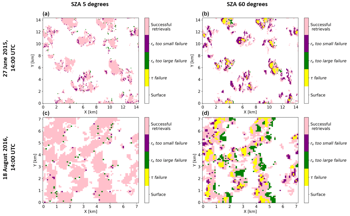
Figure A1Plots of successful and failed retrieval categories for the 27 June 2015 and 18 August 2016 cases at solar zenith angle 5° (a, c) and solar zenith angle 60° (b, d).
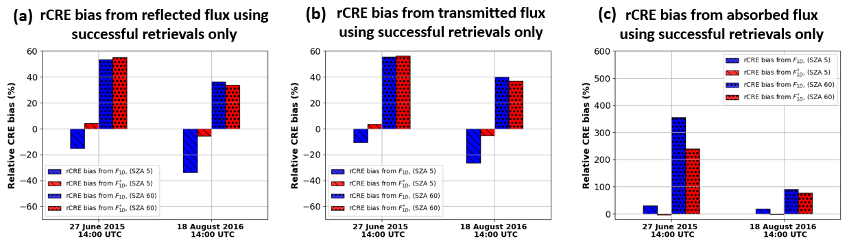
Figure A2Relative cloud radiative effect bias computed from only the successful retrievals: top of the domain reflected in panel (a), surface transmitted in panel (b), and column absorbed flux in panel (c) for the two cloud fields.
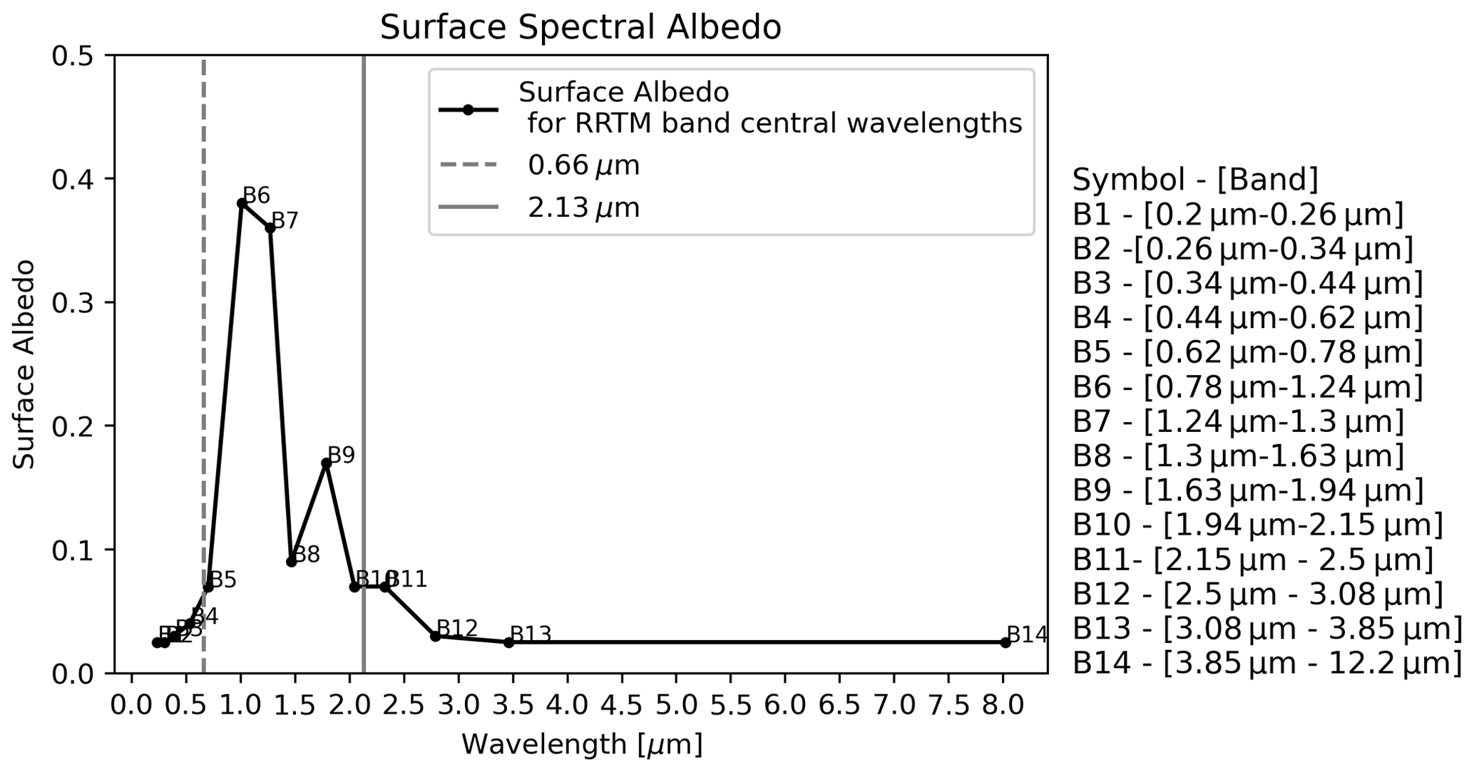
Figure B1Surface spectral albedo plot utilized in the study. Bi (i ranges from 1 to 14) represents the bands in parentheses.
The radiative transfer models and data used in the study are publicly available online. The I3RC Community Monte Carlo Radiative Transfer Model is freely available at https://github.com/RobertPincus/i3rc-monte-carlo-model (Pincus, 2009) (the I3RC Model is described in detail in the journal articles by Pincus and Evans, 2009, and Cahalan et al., 2005), while the SHDOM radiative transfer code is freely available from https://coloradolinux.com/shdom/ (SHDOM for Atmospheric Radiative Transfer is described in detail in a journal article available at https://doi.org/10.1175/1520-0469(1998)055<0429:TSHDOM>2.0.CO;2; Evans, 1998). The LASSO LES data utilized for this study are available upon request at https://archive.arm.gov/lassobrowser (ARM LASSO Bundle Browser, 2023). An overview journal article describing the LASSO activity is provided by Gustafson et al. (2020, https://doi.org/10.1175/BAMS-D-19-0065.1). The post-processed LES fields utilized as inputs for radiative transfer are available at https://doi.org/10.5281/zenodo.10511732 (Ademakinwa, 2024).
Conceptualization, ZZ; methodology, ASA, ZZ; software, ASA, ZZ; validation, ASA and ZZ; formal analysis, ASA; investigation, ASA and ZZ; data curation, ASA, ZZ; writing (original draft preparation), ASA; writing (review and editing), ASA, ZHT, JZ, CW, SP, JW, KGM, TV, and ZZ; visualization, ASA; supervision, ZZ; project administration, ZZ; funding acquisition, ZZ, JW, KGM, and CW. All authors have read and agreed to the published version of the paper.
The contact author has declared that none of the authors has any competing interests.
Publisher's note: Copernicus Publications remains neutral with regard to jurisdictional claims made in the text, published maps, institutional affiliations, or any other geographical representation in this paper. While Copernicus Publications makes every effort to include appropriate place names, the final responsibility lies with the authors.
This research has been supported by the NASA ACCESS project (grant no. 80NSSC21M0027). The computations for this study have been performed by the UMBC High Performance Computing Facility (HPCF). The facility is supported by the US National Science Foundation through the MRI program (grant nos. CNS-0821258 and CNS-1228778) and the SCREMS program (grant no. DMS-0821311), with substantial support from UMBC.
This research has been supported by the National Aeronautics and Space Administration ACCESS project (grant no. 80NSSC21M0027).
This paper was edited by Matthew Lebsock and reviewed by two anonymous referees.
Ademakinwa, A.: Dataset for manuscript “Influence of Cloud Retrieval Errors Due to Three Dimensional Radiative Effects on Calculations of Broadband Shortwave Cloud Radiative Effect”, Version v1, Zenodo [data set], https://doi.org/10.5281/zenodo.10511732, 2024.
ARM LASSO Bundle Browser: LASSO LES data, ARM [data set], https://archive.arm.gov/lassobrowser, last access: 19 May 2023.
Barker, H. W., Jerg, M. P., Wehr, T., Kato, S., Donovan, D. P., and Hogan, R. J.: A 3D cloud-construction algorithm for the EarthCARE satellite mission, Q. J. Roy. Meteor. Soc., 137, 1042–1058, https://doi.org/10.1002/qj.824, 2011.
Barker, H. W., Kato, S., and Wehr, T.: Computation of Solar Radiative Fluxes by 1D and 3D Methods Using Cloudy Atmospheres Inferred from A-train Satellite Data, Surv. Geophys., 33, 657–676, https://doi.org/10.1007/s10712-011-9164-9, 2012.
Cahalan, R. F., Oreopoulos, L., Marshak, A., Evans, K. F., Davis, A. B., Pincus, R., Yetzer, K. H., Mayer, B., Davies, R., Ackerman, T. P., Barker, H. W., Clothiaux, E. E., Ellingson, R. G., Garay, M. J., Kassianov, E., Kinne, S., Macke, A., O'Hirok, W., Partain, P. T., Prigarin, S. M., Rublev, A. N., Stephens, G. L., Szczap, F., Takara, E. E., Várnai, T., Wen, G., and Zhuravleva, T. B.: THE I3RC: Bringing Together the Most Advanced Radiative Transfer Tools for Cloudy Atmospheres, B. Am. Meteorol. Soc., 86, 1275–1294, https://doi.org/10.1175/BAMS-86-9-1275, 2005.
Cho, H.-M., Zhang, Z., Meyer, K., Lebsock, M., Platnick, S., Ackerman, A. S., Di Girolamo, L., C.-Labonnote, L., Cornet, C., Riedi, J., and Holz, R. E.: Frequency and causes of failed MODIS cloud property retrievals for liquid phase clouds over global oceans, J. Geophys. Res.-Atmos., 120, 4132–4154, https://doi.org/10.1002/2015JD023161, 2015.
Coddington, O., Pilewskie, P., Schmidt, K. S., McBride, P. J., and Vukicevic, T.: Characterizing a New Surface-Based Shortwave Cloud Retrieval Technique, Based on Transmitted Radiance for Soil and Vegetated Surface Types, Atmosphere, 4, 48–71, https://doi.org/10.3390/atmos4010048, 2013.
Davis, A. B. and Marshak, A.: Multiple Scattering in Clouds: Insights from Three-Dimensional Diffusion/P1 Theory, Nucl. Sci. Eng., 137, 251–280, https://doi.org/10.13182/NSE01-A2190, 2001.
Di Giuseppe, F. and Tompkins, A. M.: Three-dimensional radiative transfer in tropical deep convective clouds, J. Geophys. Res.-Atmos., 108, 4741, https://doi.org/10.1029/2003JD003392, 2003.
Evans, K. F.: The Spherical Harmonics Discrete Ordinate Method for Three-Dimensional Atmospheric Radiative Transfer, J. Atmos. Sci., 55, 429–446, https://doi.org/10.1175/1520-0469(1998)055<0429:TSHDOM>2.0.CO;2, 1998 (code available at: https://coloradolinux.com/shdom/, last access: 20 December 2022).
Gristey, J. J., Feingold, G., Glenn, I. B., Schmidt, K. S., and Chen, H.: Surface Solar Irradiance in Continental Shallow Cumulus Fields: Observations and Large-Eddy Simulation, J. Atmos. Sci., 77, 1065–1080, https://doi.org/10.1175/JAS-D-19-0261.1, 2020.
Gristey, J. J., Feingold, G., Schmidt, K. S., and Chen, H.: Influence of Aerosol Embedded in Shallow Cumulus Cloud Fields on the Surface Solar Irradiance, J. Geophys. Res.-Atmos., 127, e2022JD036822, https://doi.org/10.1029/2022JD036822, 2022.
Gustafson, W. I., Vogelmann, A. M., Li, Z., Cheng, X., Dumas, K. K., Endo, S., Johnson, K. L., Krishna, B., Fairless, T., and Xiao, H.: The Large-Eddy Simulation (LES) Atmospheric Radiation Measurement (ARM) Symbiotic Simulation and Observation (LASSO) Activity for Continental Shallow Convection, B. Am. Meteorol. Soc., 101, E462–E479, https://doi.org/10.1175/BAMS-D-19-0065.1, 2020.
Hogan, R. J., Fielding, M. D., Barker, H. W., Villefranque, N., and Schäfer, S. A. K.: Entrapment: An Important Mechanism to Explain the Shortwave 3D Radiative Effect of Clouds, J. Atmos. Sci., 76, 2123–2141, https://doi.org/10.1175/JAS-D-18-0366.1, 2019.
Kato, S., Rose, F. G., Sun-Mack, S., Miller, W. F., Chen, Y., Rutan, D. A., Stephens, G. L., Loeb, N. G., Minnis, P., Wielicki, B. A., Winker, D. M., Charlock, T. P., Stackhouse Jr., P. W., Xu, K.-M., and Collins, W. D.: Improvements of top-of-atmosphere and surface irradiance computations with CALIPSO-, CloudSat-, and MODIS-derived cloud and aerosol properties, J. Geophys. Res.-Atmos., 116, D19209, https://doi.org/10.1029/2011JD016050, 2011.
Kay, J. E., Hillman, B. R., Klein, S. A., Zhang, Y., Medeiros, B., Pincus, R., Gettelman, A., Eaton, B., Boyle, J., Marchand, R., and Ackerman, T. P.: Exposing Global Cloud Biases in the Community Atmosphere Model (CAM) Using Satellite Observations and Their Corresponding Instrument Simulators, J. Climate, 25, 5190–5207, https://doi.org/10.1175/JCLI-D-11-00469.1, 2012.
Kiehl, J. T. and Trenberth, K. E.: Earth's Annual Global Mean Energy Budget, B. Am. Meteorol. Soc., 78, 197–208, https://doi.org/10.1175/1520-0477(1997)078<0197:EAGMEB>2.0.CO;2, 1997.
Levis, A., Schechner, Y. Y., Aides, A., and Davis, A. B.: Airborne Three-Dimensional Cloud Tomography, in: 2015 IEEE International Conference on Computer Vision (ICCV), Santiago, Chile, 7–13 December 2015, IEEE, 3379–3387, https://doi.org/10.1109/ICCV.2015.386, 2015.
Liou, K. N.: Radiation and cloud processes in the atmosphere: Theory, observation and modeling, Oxford University Press, 487 pp., ISBN 9780195049107, 1992.
Loeb, N. G. and Manalo-Smith, N.: Top-of-Atmosphere Direct Radiative Effect of Aerosols over Global Oceans from Merged CERES and MODIS Observations, J. Climate, 18, 3506–3526, https://doi.org/10.1175/JCLI3504.1, 2005.
Loveridge, J., Levis, A., Di Girolamo, L., Holodovsky, V., Forster, L., Davis, A. B., and Schechner, Y. Y.: Retrieving 3D distributions of atmospheric particles using Atmospheric Tomography with 3D Radiative Transfer – Part 1: Model description and Jacobian calculation, Atmos. Meas. Tech., 16, 1803–1847, https://doi.org/10.5194/amt-16-1803-2023, 2023.
Marshak, A. and Davis, A. B. (Eds.): Horizontal Fluxes and Radiative Smoothing, in: 3D Radiative Transfer in Cloudy Atmospheres, Springer Berlin Heidelberg, Berlin, Heidelberg, 543–586, https://doi.org/10.1007/3-540-28519-9_12, 2005.
Marshak, A., Platnick, S., Várnai, T., Wen, G., and Cahalan, R. F.: Impact of three-dimensional radiative effects on satellite retrievals of cloud droplet sizes, J. Geophys. Res.-Atmos., 111, D09207, https://doi.org/10.1029/2005JD006686, 2006.
Masuda, R., Iwabuchi, H., Schmidt, K. S., Damiani, A., and Kudo, R.: Retrieval of Cloud Optical Thickness from Sky-View Camera Images using a Deep Convolutional Neural Network based on Three-Dimensional Radiative Transfer, Remote Sens.-Basel, 11, 1962, https://doi.org/10.3390/rs11171962, 2019.
Miller, D. J., Zhang, Z., Ackerman, A. S., Platnick, S., and Baum, B. A.: The impact of cloud vertical profile on liquid water path retrieval based on the bispectral method: A theoretical study based on large-eddy simulations of shallow marine boundary layer clouds, J. Geophys. Res.-Atmos., 121, 4122–4141, https://doi.org/10.1002/2015JD024322, 2016.
Miller, D. J., Zhang, Z., Platnick, S., Ackerman, A. S., Werner, F., Cornet, C., and Knobelspiesse, K.: Comparisons of bispectral and polarimetric retrievals of marine boundary layer cloud microphysics: case studies using a LES–satellite retrieval simulator, Atmos. Meas. Tech., 11, 3689–3715, https://doi.org/10.5194/amt-11-3689-2018, 2018.
Mlawer, E. J., Taubman, S. J., Brown, P. D., Iacono, M. J., and Clough, S. A.: Radiative transfer for inhomogeneous atmospheres: RRTM, a validated correlated-k model for the longwave, J. Geophys. Res.-Atmos., 102, 16663–16682, https://doi.org/10.1029/97JD00237, 1997.
Morrison, H. and Gettelman, A.: A new two-moment bulk stratiform cloud microphysics scheme in the Community Atmosphere Model, version 3 (CAM3). Part I: Description and numerical tests, J. Climate, 21, 3642–3659, 2008.
Nakajima, T. and King, M. D.: Determination of the Optical Thickness and Effective Particle Radius of Clouds from Reflected Solar Radiation Measurements. Part I: Theory, J. Atmos. Sci., 47, 1878–1893, https://doi.org/10.1175/1520-0469(1990)047<1878:DOTOTA>2.0.CO;2, 1990.
Nam, C., Bony, S., Dufresne, J. L., and Chepfer, H.: The 'too few, too bright' tropical low-cloud problem in CMIP5 models, Geophys. Res. Lett., 39, L21801, https://doi.org/10.1029/2012GL053421, 2012.
Nataraja, V., Schmidt, S., Chen, H., Yamaguchi, T., Kazil, J., Feingold, G., Wolf, K., and Iwabuchi, H.: Segmentation-based multi-pixel cloud optical thickness retrieval using a convolutional neural network, Atmos. Meas. Tech., 15, 5181–5205, https://doi.org/10.5194/amt-15-5181-2022, 2022.
Okamura, R., Iwabuchi, H., and Schmidt, K. S.: Feasibility study of multi-pixel retrieval of optical thickness and droplet effective radius of inhomogeneous clouds using deep learning, Atmos. Meas. Tech., 10, 4747–4759, https://doi.org/10.5194/amt-10-4747-2017, 2017.
Okata, M., Nakajima, T., Suzuki, K., Inoue, T., Nakajima, T. Y., and Okamoto, H.: A study on radiative transfer effects in 3-D cloudy atmosphere using satellite data, J. Geophys. Res.-Atmos., 122, 443–468, https://doi.org/10.1002/2016JD025441, 2017.
Oreopoulos, L., Cho, N., Lee, D., and Kato, S.: Radiative effects of global MODIS cloud regimes, J. Geophys. Res.-Atmos., 121, 2299–2317, https://doi.org/10.1002/2015JD024502, 2016.
O'Hirok, W. and Gautier, C.: A Three-Dimensional Radiative Transfer Model to Investigate the Solar Radiation within a Cloudy Atmosphere. Part I: Spatial Effects, J. Atmos. Sci., 55, 2162–2179, https://doi.org/10.1175/1520-0469(1998)055<2162:ATDRTM>2.0.CO;2, 1998.
Pincus, R.: The I3RC Community Monte Carlo Radiative Transfer Model, GitHub [code], https://github.com/RobertPincus/i3rc-monte-carlo-model (last access: 1 March 2024), 2009.
Pincus, R. and Evans, K. F.: Computational Cost and Accuracy in Calculating Three-Dimensional Radiative Transfer: Results for New Implementations of Monte Carlo and SHDOM, J. Atmos. Sci., 66, 3131–3146, https://doi.org/10.1175/2009JAS3137.1, 2009.
Platnick, S., King, M. D., Ackerman, S. A., Menzel, W. P., Baum, B. A., Riedi, J. C., and Frey, R. A.: The MODIS cloud products: algorithms and examples from Terra, IEEE T. Geosci. Remote, 41, 459–473, https://doi.org/10.1109/TGRS.2002.808301, 2003.
Platnick, S., Meyer, K. G., King, M. D., Wind, G., Amarasinghe, N., Marchant, B., Arnold, G. T., Zhang, Z., Hubanks, P. A., and Holz, R. E.: The MODIS cloud optical and microphysical products: Collection 6 updates and examples from Terra and Aqua, IEEE T. Geosci. Remote, 55, 502–525, 2016.
Rajapakshe, C. and Zhang, Z.: Using polarimetric observations to detect and quantify the three-dimensional radiative transfer effects in passive satellite cloud property retrievals: Theoretical framework and feasibility study, J. Quant. Spectrosc. Ra., 246, 106920, https://doi.org/10.1016/j.jqsrt.2020.106920, 2020.
Ramanathan, V., Cess, R. D., Harrison, E. F., Minnis, P., Barkstrom, B. R., Ahmad, E., and Hartmann, D.: Cloud-Radiative Forcing and Climate: Results from the Earth Radiation Budget Experiment, Science, 243, 57–63, https://doi.org/10.1126/science.243.4887.57, 1989.
Rossow, W. B. and Schiffer, R. A.: Advances in Understanding Clouds from ISCCP, B. Am. Meteorol. Soc., 80, 2261–2288, https://doi.org/10.1175/1520-0477(1999)080<2261:AIUCFI>2.0.CO;2, 1999.
Singer, C. E., Lopez-Gomez, I., Zhang, X., and Schneider, T.: Top-of-Atmosphere Albedo Bias from Neglecting Three-Dimensional Cloud Radiative Effects, J. Atmos. Sci., 78, 4053–4069, https://doi.org/10.1175/JAS-D-21-0032.1, 2021.
Song, H., Zhang, Z., Ma, P.-L., Ghan, S. J., and Wang, M.: An Evaluation of Marine Boundary Layer Cloud Property Simulations in the Community Atmosphere Model Using Satellite Observations: Conventional Subgrid Parameterization versus CLUBB, J. Climate, 31, 2299–2320, https://doi.org/10.1175/JCLI-D-17-0277.1, 2018.
Stocker, T. F., Qin, D., Plattner, G.-K., Tignor, M., Allen, S. K., Boschung, J., Nauels, A., Xia, Y., Bex, V., and Midgley, P. M. (Eds.): IPCC, 2013: Climate Change 2013: The Physical Science Basis. Contribution of Working Group I to the Fifth Assessment Report of the Intergovernmental Panel on Climate Change, Cambridge University Press, Cambridge, United Kingdom and New York, NY, USA, 1535 pp., ISBN 9781107661820, 2013.
Tompkins, A. M. and Di Giuseppe, F.: Generalizing Cloud Overlap Treatment to Include Solar Zenith Angle Effects on Cloud Geometry, J. Atmos. Sci., 64, 2116–2125, https://doi.org/10.1175/JAS3925.1, 2007.
Trenberth, K. E., Fasullo, J. T., and Kiehl, J.: Earth's Global Energy Budget, B. Am. Meteorol. Soc., 90, 311–324, https://doi.org/10.1175/2008BAMS2634.1, 2009.
Vardavas, I. and Taylor, F.: Radiation and Climate: Atmospheric energy budget from satellite remote sensing, International Series of Monographs on Physics, 138, Oxford University Press, Oxford, UK, 512 pp., ISBN 9780199697144, 2011.
Várnai, T.: Influence of Three-Dimensional Radiative Effects on the Spatial Distribution of Shortwave Cloud Reflection, J. Atmos. Sci., 57, 216–229, https://doi.org/10.1175/1520-0469(2000)057<0216:IOTDRE>2.0.CO;2, 2000.
Várnai, T. and Davies, R.: Effects of Cloud Heterogeneities on Shortwave Radiation: Comparison of Cloud-Top Variability and Internal Heterogeneity, J. Atmos. Sci., 56, 4206–4224, https://doi.org/10.1175/1520-0469(1999)056<4206:EOCHOS>2.0.CO;2, 1999.
Várnai, T. and Marshak, A.: Statistical Analysis of the Uncertainties in Cloud Optical Depth Retrievals Caused by Three-Dimensional Radiative Effects, J. Atmos. Sci., 58, 1540–1548, https://doi.org/10.1175/1520-0469(2001)058<1540:SAOTUI>2.0.CO;2, 2001.
Várnai, T. and Marshak, A.: Observations of Three-Dimensional Radiative Effects that Influence MODIS Cloud Optical Thickness Retrievals, J. Atmos. Sci., 59, 1607–1618, https://doi.org/10.1175/1520-0469(2002)059<1607:OOTDRE>2.0.CO;2, 2002.
Várnai, T. and Marshak, A.: View angle dependence of cloud optical thicknesses retrieved by Moderate Resolution Imaging Spectroradiometer (MODIS), J. Geophys. Res.-Atmos., 112, D06203, https://doi.org/10.1029/2005JD006912, 2007.
Welch, R. M. and Wielicki, B. A.: Stratocumulus Cloud Field Reflected Fluxes: The Effect of Cloud Shape, J. Atmos. Sci., 41, 3085–3103, https://doi.org/10.1175/1520-0469(1984)041<3085:SCFRFT>2.0.CO;2, 1984.
Wielicki, B. A., Barkstrom, B. R., Harrison, E. F., Lee, R. B., Smith, G. L., and Cooper, J. E.: Clouds and the Earth's Radiant Energy System (CERES): An Earth Observing System Experiment, B. Am. Meteorol. Soc., 77, 853–868, https://doi.org/10.1175/1520-0477(1996)077<0853:CATERE>2.0.CO;2, 1996.
Zelinka, M. D., Klein, S. A., and Hartmann, D. L.: Computing and Partitioning Cloud Feedbacks Using Cloud Property Histograms. Part II: Attribution to Changes in Cloud Amount, Altitude, and Optical Depth, J. Climate, 25, 3736–3754, https://doi.org/10.1175/JCLI-D-11-00249.1, 2012.
Zhang, Z. and Platnick, S.: An assessment of differences between cloud effective particle radius retrievals for marine water clouds from three MODIS spectral bands, J. Geophys. Res.-Atmos., 116, D20215, https://doi.org/10.1029/2011JD016216, 2011.
Zhang, Z., Ackerman, A. S., Feingold, G., Platnick, S., Pincus, R., and Xue, H.: Effects of cloud horizontal inhomogeneity and drizzle on remote sensing of cloud droplet effective radius: Case studies based on large-eddy simulations, J. Geophys. Res.-Atmos., 117, D19208, https://doi.org/10.1029/2012JD017655, 2012.
Zhang, Z., Werner, F., Cho, H. M., Wind, G., Platnick, S., Ackerman, A. S., Di Girolamo, L., Marshak, A., and Meyer, K.: A framework based on 2-D Taylor expansion for quantifying the impacts of subpixel reflectance variance and covariance on cloud optical thickness and effective radius retrievals based on the bispectral method, J. Geophys. Res.-Atmos., 121, 7007–7025, https://doi.org/10.1002/2016JD024837, 2016.
Zhang, Z., Dong, X., Xi, B., Song, H., Ma, P.-L., Ghan, S. J., Platnick, S., and Minnis, P.: Intercomparisons of marine boundary layer cloud properties from the ARM CAP-MBL campaign and two MODIS cloud products, J. Geophys. Res.-Atmos., 122, 2351–2365, https://doi.org/10.1002/2016JD025763, 2017.
Zhuravleva, T. B., Kabanov, D. M., Sakerin, S. M., and Firsov, K. M.: Simulation of aerosol direct radiative forcing under typical summer conditions of Siberia. Part 1. Method of calculation and choice of input parameters, Atmospheric and Oceanic Optics, 22, 63–73, https://doi.org/10.1134/S1024856009010102, 2009.
- Abstract
- Introduction
- Data and theory
- Results and discussion
- Summary and conclusion
- Appendix A: Impacts of failed retrievals on the radiative flux
- Appendix B: Surface spectral albedo plot
- Code and data availability
- Author contributions
- Competing interests
- Disclaimer
- Acknowledgements
- Financial support
- Review statement
- References