the Creative Commons Attribution 4.0 License.
the Creative Commons Attribution 4.0 License.
 | 05 Mar 2024
On the potential use of highly oxygenated organic molecules (HOMs) as indicators for ozone formation sensitivity
Yuanyuan Luo
Valter Mickwitz
Douglas Worsnop
Mikael Ehn
Ozone (O3), an important and ubiquitous trace gas, protects lives from harmful solar ultraviolet (UV) radiation in the stratosphere but is toxic to living organisms in the troposphere. Additionally, tropospheric O3 is a key oxidant and a source of other oxidants (e.g., OH and NO3 radicals) for various volatile organic compounds (VOCs). Recently, highly oxygenated organic molecules (HOMs) were identified as a new compound group formed from the oxidation of many VOCs, making up a significant source of secondary organic aerosol (SOA). The pathways forming HOMs from VOCs involve autoxidation of peroxy radicals (RO2), formed ubiquitously in many VOC oxidation reactions. The main sink for RO2 is bimolecular reactions with other radicals, such as HO2, NO, or other RO2, and this largely determines the structure of the end products. Organic nitrates form solely from RO2 + NO reactions, while accretion products (“dimers”) form solely from RO2 + RO2 reactions. The RO2 + NO reaction also converts NO into NO2, making it a net source for O3 through NO2 photolysis.
There is a highly nonlinear relationship between O3, NOx, and VOCs. Understanding the O3 formation sensitivity to changes in VOCs and NOx is crucial for making optimal mitigation policies to control O3 concentrations. However, determining the specific O3 formation regimes (either VOC-limited or NOx-limited) remains challenging in diverse environmental conditions. In this work we assessed whether HOM measurements can function as a real-time indicator for the O3 formation sensitivity based on the hypothesis that HOM compositions can describe the relative importance of NO as a terminator for RO2. Given the fast formation and short lifetimes of low-volatility HOMs (timescale of minutes), they describe the instantaneous chemical regime of the atmosphere. In this work, we conducted a series of monoterpene oxidation experiments in our chamber while varying the concentrations of NOx and VOCs under different NO2 photolysis rates. We also measured the relative concentrations of HOMs of different types (dimers, nitrate-containing monomers, and non-nitrate monomers) and used ratios between these to estimate the O3 formation sensitivity. We find that for this simple system, the O3 sensitivity could be described very well based on the HOM measurements. Future work will focus on determining to what extent this approach can be applied in more complex atmospheric environments. Ambient measurements of HOMs have become increasingly common during the last decade, and therefore we expect that there are already a large number of groups with available data for testing this approach.
- Article
(11726 KB) - Full-text XML
- BibTeX
- EndNote


Ozone (O3), as a key trace gas in the atmosphere, directly and indirectly affects human lives, and it plays diametrically opposing roles in the troposphere (“bad” ozone) and stratosphere (“good” ozone) (Sandermann, 1996; Staehelin et al., 2001; Seviour, 2022). The formation and depletion of O3 have been investigated over the past decades (Chapman, 1930; Crutzen, 1970, 1971; Stolarski and Cicerone, 1974; Tiao et al., 1975; Dodge, 1977). Atmospheric O3 is almost entirely produced through the reaction between atomic oxygen (O3P) and molecular oxygen (O2) (Wang et al., 2017). In the stratosphere, the O3P source is O2 photolysis with ultraviolet (UV) wavelengths below 240 nm (Chapman, 1930). Stratospheric O3, which constitutes approximately 90 % of Earth's atmospheric O3, plays a crucial role in absorbing UV radiation in the UVB band (280–315 nm), protecting organisms on the ground from harmful UV radiation (Gruijl and Leun, 2000; Seinfeld and Pandis, 2016). Although certain man-made substances, such as chlorofluorocarbons, were found to be responsible for significant depletion of stratospheric O3, the implementation of the 1987 Montreal Protocol and its subsequent amendments has contributed to the recovery of the stratospheric O3 layer (Seinfeld and Pandis, 2016; Chipperfield et al., 2017).
In the troposphere, in addition to its role as a greenhouse gas (Ehhalt et al., 2001), O3 serves as a secondary air pollutant due to its detrimental impacts and indirect emissions (Seinfeld and Pandis, 2016; Nuvolone et al., 2018). Not only is it toxic, but it also participates in chemical reactions that lead to the formation of other harmful molecules (Nuvolone et al., 2018). In contrast to stratospheric O3 in the troposphere, the source of O3P is NO2 photolysis at wavelengths less than 420 nm (Madronich et al., 1983). However, the net formation of tropospheric O3 occurs through chemical reactions involving nitrogen oxides (NOx = NO + NO2) and various volatile organic compounds (VOCs) in the presence of UV light (Lelieveld and Dentener, 2000). In an ideal “clean” system without any VOCs, once O3 is formed, it readily converts NO back to NO2 by reacting with NO, resulting in a null cycle as shown below (also illustrated as the NOx cycle in Fig. A1).
When VOCs are present, they will be oxidized to form peroxy radicals (RO2) by atmospheric oxidants, such as O3 and OH (Atkinson and Arey, 2003).
The RO2 radicals can thus replace O3 in converting NO into NO2 (Reaction R4a). Some fraction of RO2 + NO reactions will also lead to the formation of organic nitrates, RONO2 (Reaction R4b) (Atkinson and Arey, 2003).
In summary, the presence of RO2 radicals, supplied by VOCs, can perturb the NOx cycle, leading to a net increase in O3 (Fig. A1). As one of the most characteristic features of photochemical smog episodes in many cities (Tiao et al., 1975; Tang et al., 1995; Dickerson et al., 1997), this O3 formation process (Reactions R1–R4a, Fig. A1), known as O3–NOx–VOC sensitivity or O3 formation sensitivity, has been investigated since the last century (Haagen-Smit et al., 1953; Kinosian, 1982). The empirical kinetic modeling approach (EKMA) curve, namely O3 isopleths, was proposed by Dodge (1977) and has been widely used to visually study the O3 formation sensitivity (Liu and Shi, 2021). The O3 isopleths reveal a highly nonlinear response of O3 to its precursors, demonstrating that increasing or decreasing either VOCs or NOx does not consistently exhibit the same behavior regarding their impact on O3 formation (Meyer et al., 1977; Harris et al., 1982; Sillman et al., 1990). The outcome is dependent on the relative concentrations of VOCs (as a surrogate for RO2) and NOx, leading to the division of the formation area into NOx-limited and VOC-limited regimes (Sillman, 1999; Melkonyan and Kuttler, 2012). In the NOx-limited regime, the concentration of O3 generally increases with an increase in NOx, while its response to VOC changes remains relatively small. This is because the supply of RO2 species from VOCs is abundant and Reaction (R4a) is limited by NO (the NOx cycle is saturated in Fig. A1). Conversely, in the VOC-limited regime, an increase in VOC concentration generally leads to an increase in O3, whereas an increase in NOx may even result in a decrease in O3 levels. This is because NOx is in excess compared to RO2. Moreover, very high levels of NOx can directly titrate O3 (Sillman, 1999) or consume OH radicals (Atkinson et al., 2004), thereby reducing the supply of RO2 species (Reaction R3) and promoting Reaction (R2), which results in a decrease in the O3 concentration. These effects were demonstrated by amplified O3 pollution in cities during the COVID-19 lockdown, when NOx emissions dropped dramatically (Sicard et al., 2020).
To mitigate the uncertainties associated with photochemical models and efficiently determine the O3 formation sensitivity, various photochemical indicators have been utilized since the last century (Wang et al., 2017; Liu and Shi, 2021). For example, the O3 production efficiency (OPE = ) is defined as the number of O3 molecules produced per molecule of NOx before the NOx is oxidized to more stable products, i.e., NOz species (Trainer et al., 1993; Wang et al., 2017). Smaller values of OPE indicate the inefficiency of the NOx cycle (Fig. A1), suggesting that the supply of RO2 from VOCs becomes the limiting factor. As a result, the photochemical system tends to be VOC-limited. Conversely, when OPE values are higher, the system tends to be NOx-limited. Additionally, several modifications have been made to the OPE indicator to account for different situations, such as replacing ΔO3 with ΔOx (Ox = O3 + NO2) (Kleinman et al., 2002) and replacing ΔNOz with ΔNOy (NOy = NOz + NOx) (Wang et al., 2006). Other chemical species have also been utilized as photochemical indicators, including the ratio of H2O2 to HNO3 (Hammer et al., 2002). High values of indicate high potential for cross-reactions of two HO2 radicals, which is associated with high and thus indicative of the NOx-limited regime. For a more widespread application, space-based measurements from global O3 monitoring satellites have been introduced as an indicator (Martin et al., 2004) based on the fact that levels of HCHO and NO2 in the tropospheric column are closely linked to VOC and NOx emissions, respectively. However, all these indicators are not inherently linked to the O3 formation process, and the corresponding threshold values depend on environmental conditions (Liu and Shi, 2021). This makes it challenging to universally apply these indicators.
During the past decade, highly oxygenated organic molecules (HOMs) have been recognized as a new group of VOC oxidation products, particularly important for the formation of secondary organic aerosol (SOA) due to their fast formation and low volatilities (Ehn et al., 2014; Bianchi et al., 2019). Aerosols play a significant role in both impacting human health adversely (Kelly and Fussell, 2015) and influencing climate (Boucher et al., 2013). Formed in the atmosphere-mimicking gas phase and containing six or more oxygen atoms (Bianchi et al., 2019), HOMs are produced via RO2 autoxidation, which rapidly increases their oxygen content through intramolecular H atom abstractions followed by O2 additions (Crounse et al., 2013; Ehn et al., 2014). Eventually, these highly oxygenated RO2 will generally be terminated similarly as other RO2, such as through bimolecular reactions with NOx, RO2, or HO2 radicals (i.e., Reactions R4–R6).
The O3 formation precursors, namely NOx and VOCs, are thus also intrinsically connected to HOM formation through RO2 chemistry. As such, if the daytime HOM distribution is dominated by organic nitrates, it suggests that the majority of RO2 is being terminated by reactions with NO (Reaction R4), thus contributing to O3 formation. On the other hand, if we observe large quantities of HOM dimers or non-nitrate monomers, formed from RO2 + (Reactions R5 and R6), there must be a large fraction of RO2 that does not contribute to the O3 formation process, suggesting that increased NOx would also lead to more O3. In other words, ratios of different types of HOMs can function as another indicator for determining the sensitivity of O3 formation. The situation is complicated by several factors, including challenges in identifying which HOMs might have formed from RO2 termination by RO2 or HO2 and knowing if a HOM is a monomeric product of a larger VOC precursor or a dimeric product from smaller VOCs. Still, if HOMs could be used even as a qualitative indicator for O3 formation, one particular benefit would be that they would serve as a real-time indicator. This is because both the formation (through autoxidation) and loss (through condensation onto aerosol particles) of HOMs take place on timescales of minutes or less.
In this study, our objective is to assess the viability of using the ratio of HOM dimers or non-nitrate monomers to HOM organic nitrates as an indicator of O3 formation sensitivity. We conducted a series of experiments in an atmosphere simulation chamber (Riva et al., 2019a), focusing on the ozonolysis of α-pinene, the most abundantly emitted monoterpene (Pathak et al., 2007). By varying the concentrations of O3 formation precursors NOx and α-pinene, as well as the NO2 photolysis rate, we explored the shift between NOx-limited and VOC-limited regimes in the chemical system. We employed mass spectrometers and gas monitors to measure HOM products, α-pinene, O3, and NOx. We also developed a simple 0-D box model to simulate the concentrations of O3 and its precursors in the chamber under different conditions. Finally, by analyzing both experimental and model outcomes, we evaluated the potential of the HOM ratios as indicators of O3 formation sensitivity (either VOC-limited or NOx-limited) in this system.
2.1 Experiments
The experiments were conducted in the COALA chamber, as presented by Riva et al. (2019a). The cuboid chamber is made of fluorinated ethylene propylene (FEP) and has a volume of 2 m3 with a volume to surface area ratio of 0.2. The chamber was run in “steady-state mode” (Peräkylä et al., 2020; Krechmer et al., 2020), meaning there was a continuous flow of air and reagents (O3, NO2, and α-pinene) through the chamber. The total flow was around 55 L min−1, giving an average residence time of approximately 36 min ( 36 min). Each stage, where the experimental conditions remain unchanged, lasted at least 1.5 h, which is approximately 3 times the residence time, allowing the chamber to reach a pseudo-steady state, as confirmed by the time series obtained during the experiments (e.g., Fig. 4).
Table 1Experimental conditions. Each experiment consisted of three to nine “stages” that corresponded to a specific time period during which the inputs remained constant. The parameter that was varied included input O3, α-pinene, or NOx concentrations, as well as NO2 photolysis rate (). These variations are indicated in the table by multiple values or ranges in a given cell. The experiment number (no.) and number of total stages per experiment are shown in the first two columns.
The details of the conducted experiments are provided in Table 1. The UV LED lights (wavelength ∼ 400 nm, manufactured by LEDlightmake Inc., Shenzhen, China) (Zhao et al., 2023a) used for photolyzing NO2 were kept on throughout each experiment, while the input concentrations of the precursors NO2, O3, and α-pinene were varied across experiments and stages to map out a wide range of different conditions. The photolysis rate was varied by using varying numbers of LED light strips (one, three, or five). Experiments without VOC addition (nos. Z1–Z5, Table A1) were used to evaluate the photolysis rates (given in Table 1) for each number of light strips. We acknowledge that using alkene ozonolysis for this type of study is not ideal as O3 also reacts with the VOCs, making the determination of actual O3 formation more complicated. The choice of this system was partly due to our chamber not having the optimal light source for producing OH radicals, thus limiting us to O3 oxidation, and partly because the HOM spectra from this system have been studied in great detail, making the interpretation of the HOMs easier.
All the input reactants, as well as the HOM products, were continuously measured online using instruments described below. The identified HOM species in this study were categorized into three groups: (1) HOM monomers (HOMMono), which are C8–C10 compounds without any nitrogen atoms; (2) HOM organic nitrates (HOMON), which are C8–C10 compounds with one nitrogen atom; and (3) HOM dimers (HOMDi), which are C18–C20 compounds without any nitrogen atoms.
2.2 Instrumentation
2.2.1 Mass spectrometers
A nitrate-adduct chemical ionization mass spectrometer (NO3-CIMS, Tofwerk AG/Aerodyne Research, Inc.) was used for online measurements of HOMs with high selectivity (Jokinen et al., 2012; Ehn et al., 2014; Riva et al., 2019b). A large sheath flow of 20 L min−1 (to minimize wall losses) carries nitric acid (HNO3) across X-rays, producing nitrate ions (). Then, in an electric field, is guided towards a 10 L min−1 sample flow, ionizing targeted HOM molecules by clustering with them (Kürten et al., 2014). Finally, the charged sample molecules are directed through a critical orifice and into an atmospheric pressure interface time-of-flight mass spectrometer (APi-TOF), where they are detected based on mass-to-charge ratios () (Junninen et al., 2010). The NO3-CIMS was equipped with a standard TOF (HTOF), having a mass resolution of 5000 at 188 Th. The concentrations of HOMs were converted from their normalized signals (i.e., the ratio of HOM-containing ions to reagent ions) by multiplying with a calibration factor (C), which takes different efficiencies into account (Jokinen et al., 2012; Bianchi et al., 2019).
Calibrating with sulfuric acid (Kürten et al., 2012), we determined C to be 1.56 × 109 cm−3 (± 50 %) based on a flow-tube model (He et al., 2023). However, in this study, the accuracy of C is less important since the normalized signals of HOMs were sufficient for relative comparisons.
A proton transfer reaction time-of-flight mass spectrometer (PTR-TOF 8000, Ionicon Analytik GmbH), designed for online measurements of VOCs (Jordan et al., 2009), was utilized in our study specifically for the detection of α-pinene. The PTR is an ionization method where water molecules (H2O) are ionized in a hollow cathode discharge, resulting in the formation of hydronium ions (H3O+) (Hansel et al., 1995). Then, as proton donors, H3O+ is directed into a drift tube, where trace organic compounds are ionized by proton transfer process with proton affinity as the key parameter (Hansel et al., 1995; Graus et al., 2010). After a differentially pumped ion transfer unit, the charged molecules enter a TOF, where collisions are negligible under a low pressure of ∼ 10−6 mbar with a high vacuum (Graus et al., 2010). The inlet flow was 1 L min−1 with 0.1 L min−1 being sampled into the ion drift tube. Further details regarding the calibration and settings of the PTR can be found in Zhao et al. (2023b), and the calibration factor for α-pinene (detected as at 137 Th) was ∼ 104 ppb−1 after normalization by primary ion isotope (at 21 Th). The analysis of raw data from the NO3-CIMS and PTR-TOF was conducted using the MATLAB-based set of programs called tofTools (version 611) (Junninen et al., 2010).
2.2.2 Gas monitors
The concentrations of NOx and O3 were measured by gas monitors. A photometric O3 analyzer – model 400 (Teledyne API) was used to detect O3 in the chamber. The amount of O3 determines how much of a 254 nm UV light signal is absorbed in the sample cell. The absorption difference between the intact sample air and the O3-removed air, achieved by a switching valve periodically, enables the determination of the stable O3 concentrations.
As for NOx, an NO–NO2 analyzer – model T200UP (Teledyne API) – was utilized. With a high-efficiency photolytic converter, NO2 is transformed to NO with minimal interference from other gases. Using the chemiluminescence detection principle, NO is measured by reacting with O3, yielding light in direct proportion to the amount of NO (Archer et al., 1995). In this way, both sampled NO and total NOx can be measured, without and with using the photolytic converter, respectively. This enables the determination of the NO2 concentration in the sample by subtraction.
2.3 Box model
As O3 was both injected and produced in the chamber, and sinks included reactions with NO and VOCs as well as flush-out, we constructed a simple 0-D box model (14 reactions, Table A2) to mimic the main reactions and to generate O3 isopleth diagrams. These isopleths were then used to determine sensitivity regimes for O3 formation. Reaction rates were adapted from the NIST Chemical Kinetics Database (https://kinetics.nist.gov/kinetics/index.jsp, last access: 25 August 2023). The model did not include closed-shell HOM products and all peroxy radicals were treated as a single term (i.e., RO2). The box model was first employed to determine NO2 photolysis rates under different numbers of UV lights in the zero-VOC experiments (Table A1), where only O3 and NO2 were used as input species. The high agreement between the model and observations (detailed results are shown in Sect. 3.1 and 3.3) showed that the model was adequate for simulating the targeted reactions in our chamber.
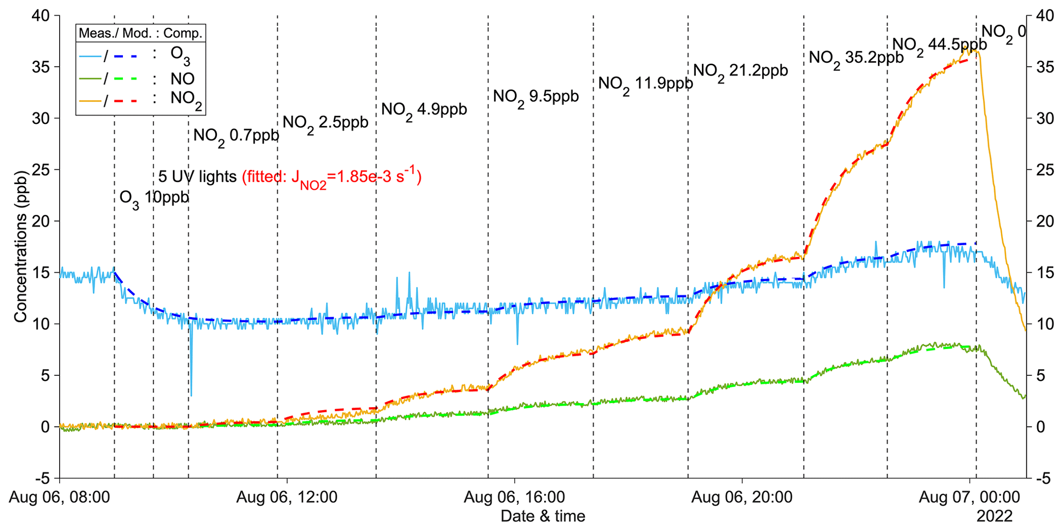
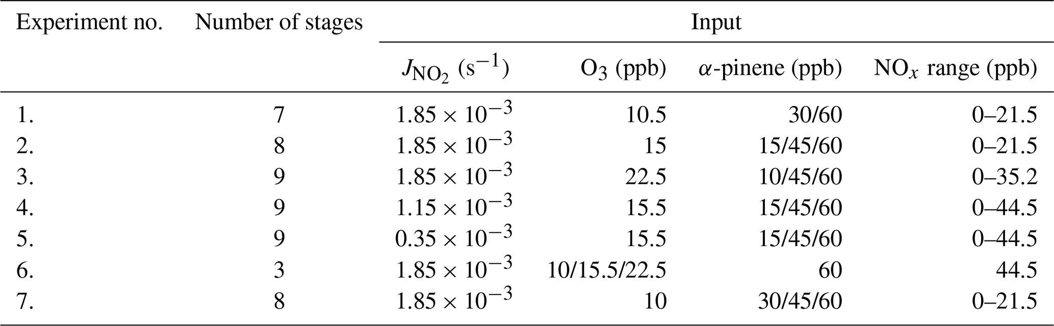
Figure 1A zero-VOC experiment (Z1) for determining the photolysis rate of NO2. Measured (abbreviated as Meas.) and modeled (abbreviated as Mod.) concentrations of different compounds (abbreviated as Comp.) are shown as solid and dashed lines, respectively. Dashed vertical lines indicate specific time points of operations, with corresponding labels for each operation. Note that the operation labels show input information (input NO2: measured NO2 + NO).
3.1 NO2 photolysis rate determination
Figure 1 illustrates an example of a zero-VOC experiment, while Table A1 provides a comprehensive list of all zero-VOC experiments conducted. Using the box model, NO2 photolysis rates () were determined by varying the parameter in the model until the simulated O3 and NOx values agreed with the observations in the zero-VOC experiments (Figs. 1 and A2–A5). With = 1.85 × 10⁻³ s−1 with five UV lights, the modeled gas concentrations agreed extremely well with measured values (Fig. 1). Similar agreement was observed for different inputs of O3 and NO2 (Figs. A2 and A3), indicating the robustness of both the model itself and the fitted . Furthermore, employing the same procedure, the photolysis rates with three UV lights and one UV light were determined to be 1.15 × 10⁻³ and 0.35 × 10⁻³ s−1, respectively (Figs. A4 and A5). The values for could also be computed from the observed steady-state and input concentrations of for each condition (details see Table A1).
Figure 2The steady-state spectrum (15 min average) at stage 7 of experiment no. 2 from the NO3-CIMS. The spectrum was corrected by subtracting the corresponding background signals. Light green bars show HOMMono, dark green ones show HOMDi, blue ones show HOMON, and grey ones show peaks not of interest. The peaks not of interest either exhibited relatively low signals, represented radicals, contained too small a number of carbon and oxygen atoms, or had uncertain mass-to-charge ratios. The peaks larger than 450 Th are multiplied by 10.
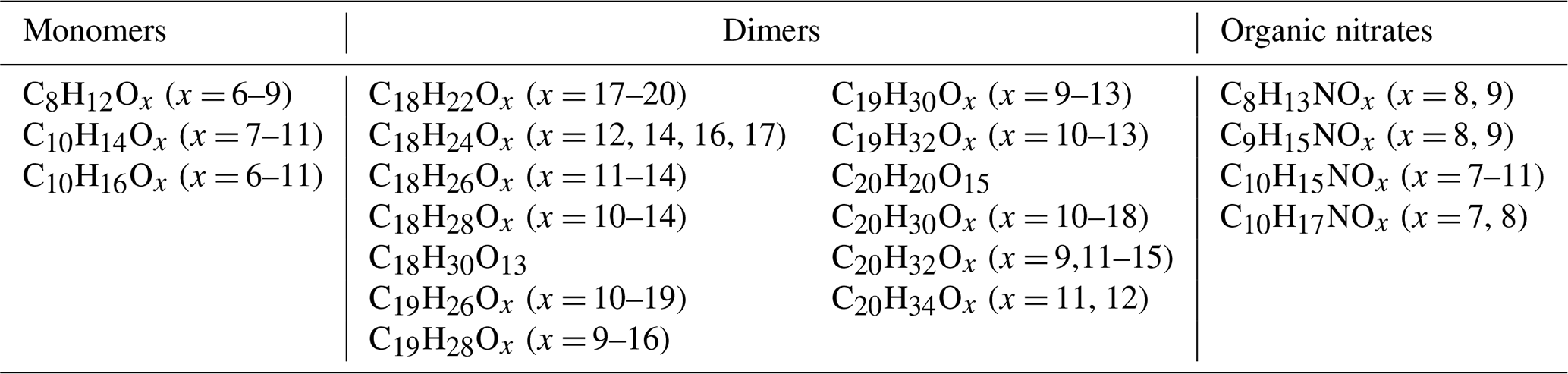
Table 2Identified HOM closed-shell species based on experiment no. 2. The reagent ion is excluded.
3.2 HOM determination
A steady-state spectrum (experiment no. 2) obtained from the NO3-CIMS (Fig. 2) illustrates the identified closed-shell HOM products, including HOMMono (light green), HOMON (blue), and HOMDi (dark green). Table 2 provides the formulas of all the selected HOM species. Figure A6 displays the steady-state spectra of all stages, with the corresponding input information described in Fig. 4a. As expected, with the injection of more NO2, the signals of HOMON increased, while those of HOMMono and HOMDi decreased considerably (stages 2–5 in Fig. A6). This observation is consistent with the dominance of the RO2 + NO reaction over the RO2 cross-reactions at a few parts per billion of NOx (Yan et al., 2016, 2020). After the addition of more α-pinene, all signals showed a noticeable rise (stages 6–7 in Fig. A6) due to the increased supply of RO2 species.
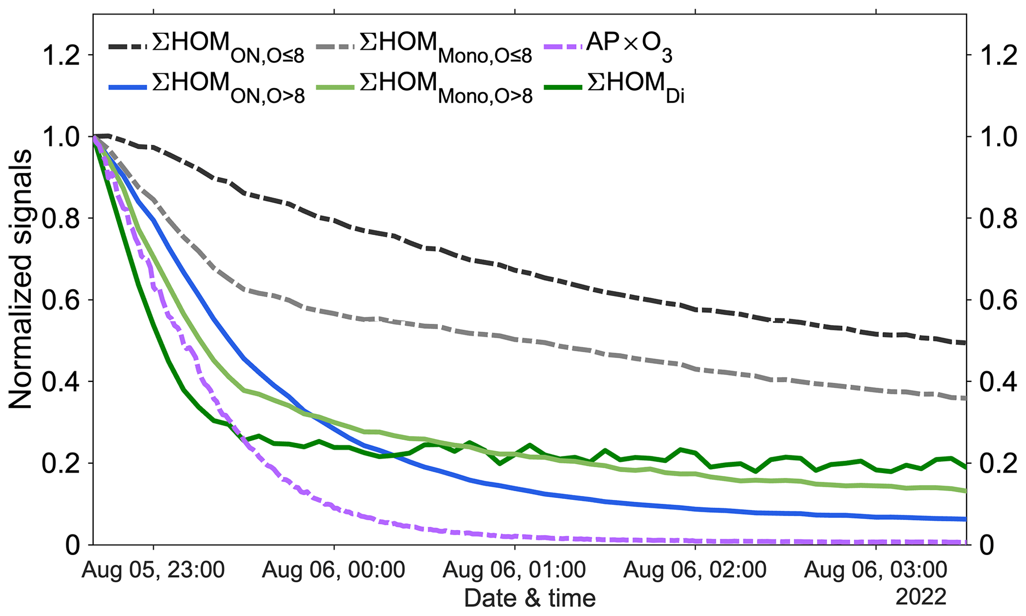
Figure 3The normalized signal decays after experiment no. 2 ended. All signals were normalized first to primary ions and then to the signals at the moment when experiment no. 2 ended. Dashed lines: ∑ HOM (sum of HOMON species with fewer than nine oxygen atoms, in black), ∑ HOM (in grey), and AP × O3 (multiplication of α-pinene and O3 concentrations, in purple). Solid lines: ∑ HOM (in blue), ∑ HOM (in light green), and ∑ HOMDi (in dark green).
Our experiments showed that HOM organic nitrates with fewer than nine oxygen atoms (HOM) exhibited the slowest decay at the end of the experiment (Fig. 3). This can be explained by the evaporation of these semi-volatile HOM compounds from chamber walls even after the gas-phase production had stopped. Additionally, non-nitrate HOM monomers with fewer than nine oxygen atoms (HOM) also showed an overall slow decay (Fig. 3). As a result, prior to subsequent experiments, the concentration levels of HOM and HOM remained high, obscuring actual concentration changes following the addition of NOx. As such, the ratios of the different compound groups are impacted by memory effects from previous experiments and wall interactions and would therefore be poor real-time indicators of the O3 formation sensitivity. In the atmosphere, the long-lived oxygenated VOCs (OVOCs) could linger for hours to days, and the ratios of, e.g., nitrates to non-nitrates would be greatly influenced by various loss terms (photolysis, oxidation, condensation, hydrolysis, etc.) that may differ dramatically between different compound groups. In contrast, HOM, HOM, and HOMDi experienced fast decays due to their very low volatilities, corresponding to lifetimes well below 1 h when accounting for the fact that HOM formation (roughly estimated by the dashed purple line in Fig. 3) continued while the precursors were being flushed out (the higher normalized background level of HOMDi is due to their lower initial concentrations, but this stable level allowed for accurate background subtraction in each experiment). Therefore, we excluded the less oxygenated and more volatile HOM species, specifically HOM and HOM, to obtain parameters with short enough lifetimes to truly reflect the ongoing chemistry in real time. The remaining differences in decay rates in Fig. 3 may also reflect slight differences in loss rates for the highly oxygenated species, but also the yields of the different compound groups are a function of, e.g., reaction rates. For example, dimer formation requires RO2 + RO2 reactions, which are more favored at higher VOC oxidation rates. Consequently, the indicating ratio used in this study is defined as the ratio between the sum of HOMDi or HOM and the sum of HOM, represented as (indicating ratio 1, abbreviated as IR1) or (IR2). We emphasize that these ratios will be specific to our experiments, as yields for the different groups will vary for different VOCs and conditions. Nevertheless, the use of the most oxidized, i.e., the least volatile, HOMs is critical in this context, as their loss rates are very similar as they all behave as if they were non-volatile, thus condensing irreversibly to surfaces as the main sink term.
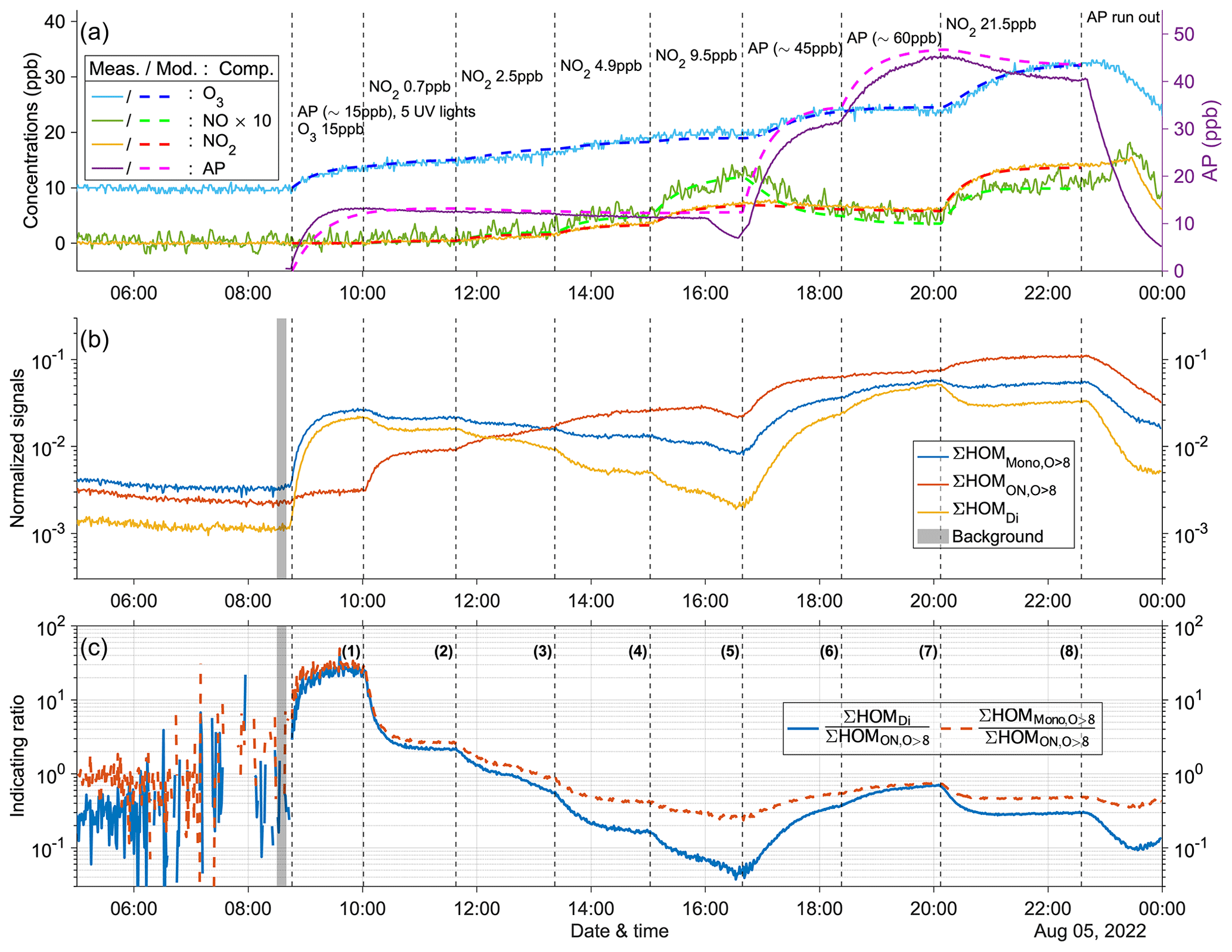
Figure 4Time series of experiment no. 2 with 15 ppb α-pinene and 15 ppb O3 as initial inputs. Five UV lights were on during all stages. Three panels show the time series of different compounds: (a) measured (abbreviated as Meas., in solid lines) and modeled (abbreviated as Mod., in dashed lines) concentrations of O3, NOx (both shown by the left y axis; the NO concentration is multiplied by 10), and AP (i.e., α-pinene, shown by the right y axis); (b) normalized signals of ∑HOM (sum of non-nitrate HOM monomers with more than eight oxygen atoms), ∑ HOM (sum of HOM organic nitrates with more than eight oxygen atoms), and ∑HOMDi (sum of HOM dimers); (c) IR1 and IR2 . The grey shaded area represents the time period selected for background subtraction before calculating the ratio. Dashed vertical lines indicate specific time points of operations, with the corresponding labels for each operation in panel (a). The bolded number in parentheses in panel (c) corresponds to the number of stages. The steady-state mass spectra obtained by the NO3-CIMS for each stage are shown in Fig. A6.
3.3 Indicating ratios
In this section, we detail the conducted experiments. Experiment no. 2 is depicted in Fig. 4, while the other experiments are shown in Figs. A7–A12. It is worth noting that our experiments did not result in notable particle formation, and condensation to walls was always the dominant loss term for HOMs. If aerosol formation had been significant, as has been observed in our chamber at higher oxidation rates (Zhao et al., 2023a), HOMs would first increase due to fast formation and then decrease due to condensation sink. Variation of NO2 and α-pinene input concentrations leads to changes in both indicating ratios (IR1 and IR2) that correspond to changes in O3 concentrations (Fig. 4), suggesting a possible sensitivity of O3 formation. From stages 1 to 5, injection of more NO2 led to increased formation of HOM, while production of HOMDi and HOM was suppressed. As a result, the indicating ratios decreased. Additionally, the concentration of O3 increased during this period, but the rate of increase decreased with higher NO2 inputs. This trend suggests a gradual shift from a NOx-limited regime to a more VOC-limited regime in the system. For example, during stage 5 with 9.5 ppb NO2, the O3 concentration remained relatively constant. This observation indicates the system may have shifted to the VOC-limited regime. Next, when additional α-pinene was introduced (∼ 45 ppb during stage 6), a significant increase in O3 concentration was again observed, consistent with the system being in the VOC-limited regime during stage 5. However, after injection of ∼ 60 ppb α-pinene during stage 7, the O3 concentration reached a plateau, indicating that the system had shifted back to the NOx-limited regime. Moreover, during these two stages, the indicating ratios experienced a substantial increase. In the last stage, stage 8, when additional NO2 was injected to reach 21.5 ppb while the input α-pinene concentration remained unchanged, the O3 concentration increased again, and the indicating ratios decreased noticeably, confirming that the previous stage was NOx-limited. However, it should be noted that the system in this stage might not yet be VOC-limited.
Other experiments with five UV lights (Figs. A7, A8, and A11) also exhibited similar time series patterns as described above. One noticeable difference is that higher initial O3 concentrations resulted in less pronounced increases in O3 during the first five stages with varying NO2 levels. This can be attributed to the reaction O3 + NO (Reaction R2) becoming faster, competing with the formation of O3 from the RO2 + NO reaction (Reaction R4a) followed by NO2 photolysis (Reaction R1). As a result, there was reduced O3 formation in the presence of higher initial O3 concentrations due to the scavenging of NO by existing O3.
Compared to experiment no. 2 (Fig. 4), experiments with fewer lights (but similar initial concentrations; Figs. A9 and A10) provide insight into the effect of UV light intensities on O3 formation sensitivity and the consistency of the indicating ratios under different light intensities. More lights led to a more pronounced increase in O3 concentrations at the same stages because additional O3 was produced from NO2 photolysis. On the other hand, fewer lights resulted in lower NO levels in the system since NO2 input was the sole source of NOx. This led to reduced NO2 formation from RO2 + NO reaction (Reaction R4a) and subsequently less O3 formation. This aspect is crucial in determining the O3 sensitivity. In this sense, the presence of fewer lights implies that higher levels of NO2 input are required to ensure sufficient NO levels for reaching the VOC-limited regime. This can be confirmed by the stage where ∼ 45 ppb α-pinene was injected (Figs. 4, A9, and A10). During this stage, the O3 concentration showed a significant increase with either three or five UV lights, indicating that the system had reached the VOC-limited regime in the previous stage. However, when only one UV light was used, the O3 concentration remained relatively constant, suggesting that the system with one light did not reach the VOC-limited regime. It is worth mentioning that the indicating ratios exhibited more significant changes when using more lights. This can be attributed to the fact that more lights result in increased production of O3 and NO, leading to more drastic changes in HOM distributions and thereby influencing the indicating ratios to a greater extent.
Using the box model described in Sect. 2.3, the concentrations of O3 and its precursors were captured well both qualitatively and quantitatively (e.g., Fig. 4a). In general, simulated concentrations of O3 during the steady states differed from measured values by at most 10 %, while differences for NOx were even smaller. The largest discrepancy in concentrations (∼ 15 %) was observed for α-pinene, which can be attributed to the simplifications made in the model. Specifically, the OH concentration will be underestimated if the model does not accurately capture the yields of HO2, which can be converted into OH via reactions with NO.
Overall, both indicating ratios are promising as indicators of O3 formation sensitivity. However, in all time series (Figs. 4c, A7c–A12c), IR1 () exhibited more pronounced changes compared to IR2 () as we shifted the O3 formation regimes. This highlights that in the well-controlled chamber systems we investigated, IR1 may hold better potential for indicating O3 formation sensitivity in the absence of other perturbing factors. It can be explained by the fact that the nitrates are solely from RO2 + NO and the dimers solely from RO2 + RO2. But HOM monomers can be from both of these reactions. On the other hand, in the real atmosphere, IR1 is expected to be much less robust, as discussed in more detail in Sect. 3.5. The intensity of light (i.e., NO2 photolysis rate) played a crucial role in determining O3 sensitivity regimes by controlling the amount of NO. Our box model successfully reproduced the measured values of O3 and its formation precursors, making it reasonable to extend the model to generate O3 isopleths under chamber conditions beyond those covered in our experiments. With these we can better elucidate how well the HOM ratios can function as O3 sensitivity indicators in this system.
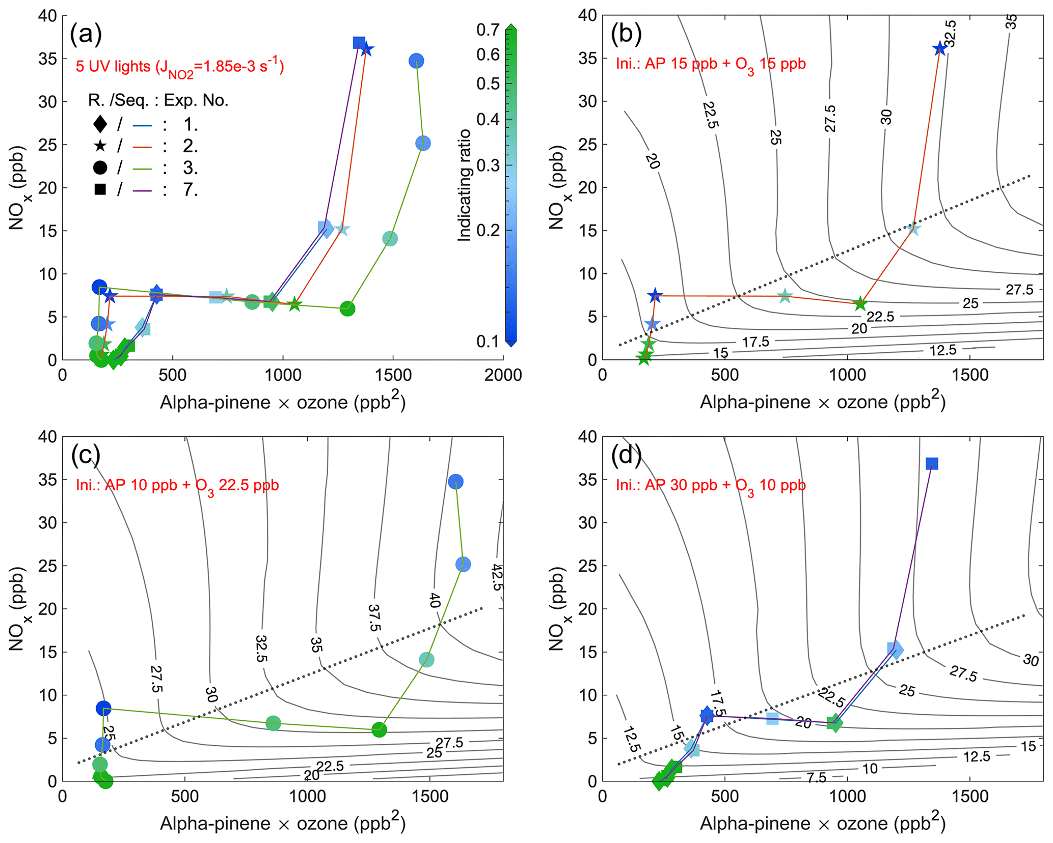
Figure 5Steady-state IR1 of experiments from 4 d with five UV lights. The x axis is the multiplication of steady-state α-pinene and O3 concentrations, while the y axis is the steady-state NOx. The scatter points (exp. no. 1: diamond; exp. no. 2: star; exp. no. 3: round; exp. no. 7: square) are colored by values of IR1 (abbreviated as R. in the figure) and are connected by curves (exp. no. 1: blue; exp. no. 2: orange; exp. no. 3: green; exp. no. 7: purple) showing the sequence (Seq.) of experimental stages. Panel (a) combines stages of all 4 d, and the other three panels respectively show the stages of experiments with different initial (Ini.) inputs (exp. nos. 1 and 7 are in the same panel (d) due to the same initial inputs). EKMA curves (isopleths of O3 concentrations in ppb), simulated by the box model, are solid black lines, while dotted lines are the corresponding ridge lines.
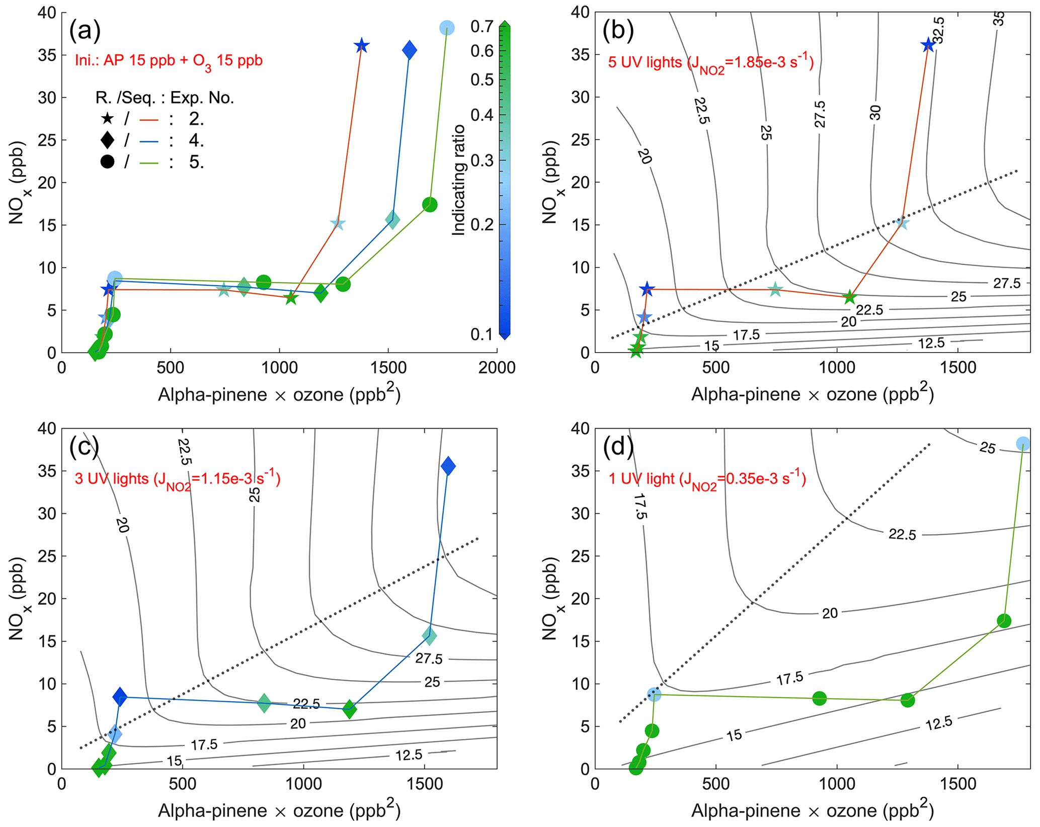
Figure 6Steady-state IR1 of experiments from 3 d with five UV lights, three UV lights, and one UV light, respectively. The x axis is the multiplication of steady-state α-pinene and O3 concentrations, while the y axis is the steady-state NOx. The scatter points (exp. no. 2: star; exp. no. 4: diamond; exp. no. 5: round) are colored by values of IR1 (abbreviated as R. in the figure) and are connected by curves (exp. no. 2: orange; exp. no. 4: blue; exp. no. 5: green) showing the sequence (Seq.) of experimental stages. Panel (a) combines stages of all 3 d with the same initial (Ini.) inputs, and the other three panels respectively show the stages of experiments with different numbers of UV lights. EKMA curves by the box model are black lines, and the dotted lines are the corresponding ridge lines.
3.4 Viability of the indicating ratios
In order to validate the indicating ratio, we generated O3 isopleths by modeling various combinations of input NO2 and α-pinene concentrations. The indicating ratios obtained from all steady-state stages were scattered on the same coordinate system (IR1: Figs. 5 and 6 and IR2: Figs. A13 and A14). The purpose of varying the injection rates of either NOx or α-pinene within each experiment (e.g., colored curves in Fig. 5) was to shift the system between the VOC-limited and NOx-limited regimes. Unlike previous studies that used the concentration of VOCs as the x axis (Kinosian, 1982; Chameides et al., 1992), in this study, the x axis represented the product of the measured α-pinene and O3 concentrations. This is because the product reflects the potential for RO2 formation, which reacts directly with NO to contribute to O3 accumulation (Reactions R1–R4a). In typical EKMA plots the oxidant is primarily thought to be OH, the concentration of which is independent of the VOC concentrations; thus, the x axis would be largely equivalent regardless of whether plotting VOCs or VOCs times oxidant. In our case, the VOC concentration will directly influence the oxidant (i.e., O3) concentration through chemical reactions, and therefore we chose to use the current x axis. The ridge line of the EKMA curves was plotted for each experiment, represented by dotted lines in, e.g., Fig. 5b–d. The reason for separating panels (b)–(d) from each other is due to the differences in constant O3 inputs or NO2 photolysis rates in each experiment, resulting in distinct O3 isopleths. For the context of this work, we do not separate a transition regime where O3 formation is sensitive to both NOx and VOCs but simply define the VOC- and NOx-limited regimes based on the ridge line. Farther above the ridge line, the system is more VOC-limited, while farther below the line, the system is more NOx-limited. It is notable that in the VOC-limited regime, instead of a reduction, the O3 concentration even increased slowly with the addition of NOx, primarily due to the photolysis of the input NO2.
Comparing experimental and model results, the steady-state stages of all experiments with five UV lights exhibited a consistent pattern for the indicating ratios, allowing qualitative determination of O3 formation sensitivity (Figs. 5 and A13). Generally, the farther the steady-state point is from the ridge line, the darker the coloring (either blue or green). Specifically, when the color is darker blue, it indicates a smaller value of the indicating ratios, suggesting a higher likelihood of the system being in the VOC-limited regime. Conversely, when the color is darker green, it signifies a higher value of the ratios, indicating a higher likelihood of the system being in the NOx-limited regime. It is worth noting that experiment no. 7 was essentially a duplicate of experiment no. 1, but with additional stages. When comparing the indicating ratios at stages with the same inputs, as shown in Figs. 5d and A13d, it becomes apparent that the values are highly consistent and closely aligned. Moreover, the background signals of HOM, HOM, and HOMDi increased substantially with experiments going on, from 5 × 10⁻⁴–2 × 10⁻³ (Fig. A7b) to 4 × 10⁻³–2 × 10⁻² (Fig. A11b). However, the accumulating background did not have a significant impact on the indicating ratios after the background subtraction (Fig. 5d and A13d). This highlights the remarkable reproducibility of the indicating ratios in our chamber experiments.
To investigate the impact of light intensities, a similar comparison was conducted for experiments with the same initial inputs using five UV lights, three UV lights, and one UV light (Figs. 6 and A14). The observed changes in the pattern of the indicating ratios are in line with those observed in the experiments with five UV lights described above. The most significant observation is that at lower UV light intensity, the ridge line shifted towards higher NOx levels at the same potential for RO2 formation (i.e., the same value of x axis) (Figs. 6b–d and A14b–d). This finding aligns with the time series comparison presented in Sect. 3.3, which indicates that at weaker UV intensity, higher input NO2 is required to generate sufficient NO levels to shift the system towards the VOC-limited regime. When comparing stages with the same conditions except different UV lights, we generally observed that a lower intensity of UV lights corresponded to higher values of the indicating ratios (Figs. 6 and A14), showing a higher likelihood of the system being in the NOx-limited regime. This finding is in agreement with the shift of the ridge line. The correlation between UV intensities, the indicating ratios, and the position of the ridge line reinforces the relationship between the indicating ratios and O3 formation sensitivity. It suggests that in addition to the relative changes, the absolute values of the indicating ratios are also informative.
The conclusion can be drawn that the indicating ratios can qualitatively predict the O3 formation regimes (either VOC- or NOx-limited). More specifically, based on modeled EKMA curves and steady-state HOM ratios (Figs. 5, 6, A13, and A14), regardless of the light intensity, IR1 and IR2 consistently indicate the VOC-limited regime when below 0.2 and 0.4 and the NOx-limited regime when above 0.5 and 0.7.
3.5 Implications and further improvements
Our chamber study (Sect. 3.4) confirmed the significant role of the indicating ratios in determining O3 formation sensitivity qualitatively. However, in the real atmosphere, the conditions will vary significantly more than in our simple system. Most importantly, the number of different precursor VOCs will be vastly greater, and in reactions with OH, the distribution of different types of RO2 radicals will also be far more complex. As an example, in a rural setting there can be a wide variety of small VOCs (C1–C4), isoprene (C5), aromatics (C6–C9), and monoterpenes (C10) that all produce significant amounts of RO2. Consequently, from these molecules, dimers can form with any carbon number between 2 and 20, while monomers can have carbon numbers between 1 and 10. In addition, both VOC and oxidant concentrations as well as radiation and meteorological patterns will vary over time. This means that it will be difficult to find universal compounds to include in the HOMDi, HOMMono, and HOMON groups used to calculate the indicating ratios for a given site and a given time. For example, it is likely that there will be few environments where C10 RO2 from monoterpenes would be efficiently reacting with each other during daytime, meaning that the C20 dimers used here are unlikely to be usable. It remains to be seen whether the HOMMono-to-HOMON ratio can be used for C10 compounds in areas with high monoterpene emissions. Nevertheless, conceptually the link between HOM formation pathways and O3 formation should hold, and it may be possible to determine suitable compound groups for various sites. Our study focused exclusively on α-pinene, but the intrinsic connection between the indicating ratios we proposed and O3 formation (Fig. A1) is not limited to this specific VOC. Further laboratory and ambient studies are necessary to investigate additional VOCs of interest and expand our understanding of the indicating ratios' applicability and generalizability in predicting O3 formation sensitivity under various atmospheric conditions. In addition, at the extremes, ranging from clear formation of dimeric species to complete lack of dimeric species with abundant organic HOM nitrates, this can be considered a strong qualitative indicator of a NOx-limited or VOC-limited regime, respectively.
Both O3 and HOMs are of significant interest, given their impacts from small-scale personal health to large-scale global climate. Due to the intrinsic connection between the formation mechanisms of O3 and HOMs, we suggest new indicators, denoted as and , for determining O3 formation regimes based on the distribution of HOMs. One main improvement of using HOM-based indicating ratios compared to those suggested earlier would be the short lifetimes of HOMs, which means that these new indicators would be real-time indicators of the formation regime. To assess the viability of the indicating ratios, a series of chamber experiments were carried out using a NO3-CIMS, a PTR-TOF, and O3 and NOx monitors. As expected, an increase in NOx inputs led to an increase in HOMON and a decrease in HOMDi, HOMMono, and the indicating ratios. Conversely, an increase in α-pinene resulted in a rise in the indicating ratios. Furthermore, when adding enough of one of the O3 formation precursors (either NOx or α-pinene), the rate of increase in O3 concentration slowed down or even stopped. This indicates that the system was shifting to or had already reached the other limited regime.
With a box model, which closely reproduced the measured concentrations of O3 and its precursors, O3 isopleths were obtained for different concentrations of NOx and α-pinene. After drawing ridge lines of the isopleths, it was observed that the indicating ratios provide a qualitative prediction of the O3 formation regimes: lower values of the ratios indicate a greater likelihood of the system being located in the VOC-limited regime, and vice versa. With less intense UV light (λ≈ 400 nm), a higher amount of NO2 was required to shift the system towards the VOC-limited regime. This can be attributed to a decrease in the formation of NO from NO2 photolysis. Nevertheless, the absolute values of the indicating ratios exhibited a consistent behavior across different intensities of UV light, suggesting that these absolute values are highly valuable for analyzing O3 formation sensitivity.
The main objective of this study was to evaluate the concept of using HOM distributions in indicating O3 formation sensitivity. Based on our outcomes, we can conclude that the ratio of HOM dimers or non-nitrate monomers to HOM organic nitrates (i.e., or ) has the capability to indicate O3 formation regimes (either VOC- or NOx-limited) in this simple system of monoterpene ozonolysis. An indicating ratio of this kind would aid in better control of O3 pollution and have the potential to be incorporated as a useful parameter into global models for analyzing O3 formation sensitivity under diverse environmental conditions.
Nevertheless, future studies will need to assess whether this approach is feasible to be applied in real-world conditions where the chemistry is far more complex. The variability of VOC precursors alone will greatly perturb the ideal situation observed in our chamber. Still, we posit that environments with high monoterpene emissions will also produce abundant C10 RO2 concentrations, and the comparison of the highly oxygenated monomeric termination products (i.e., nitrates vs. non-nitrates) can provide an indication of the relative RO2 termination pathways. Further studies, both ambient observations and chamber experiments involving multiple VOCs and oxidants will be necessary to determine the potential of HOM-based indicators for O3 formation.
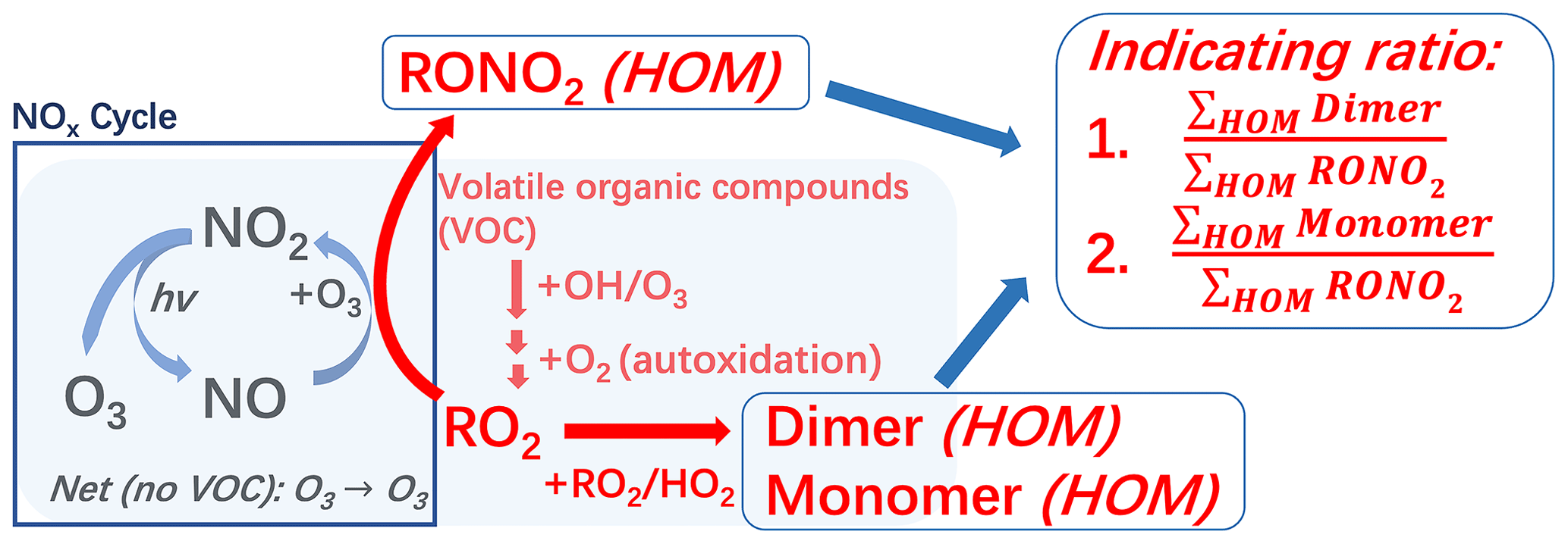
Figure A1A sketch of the connection between HOMs and O3 formation. Based on the formation connection, two indicating ratios between the HOM species are defined. RONO2 (HOM): nitrate-containing HOM monomers, dimer (HOM): non-nitrate HOM dimers, monomer (HOM): non-nitrate HOM monomers.
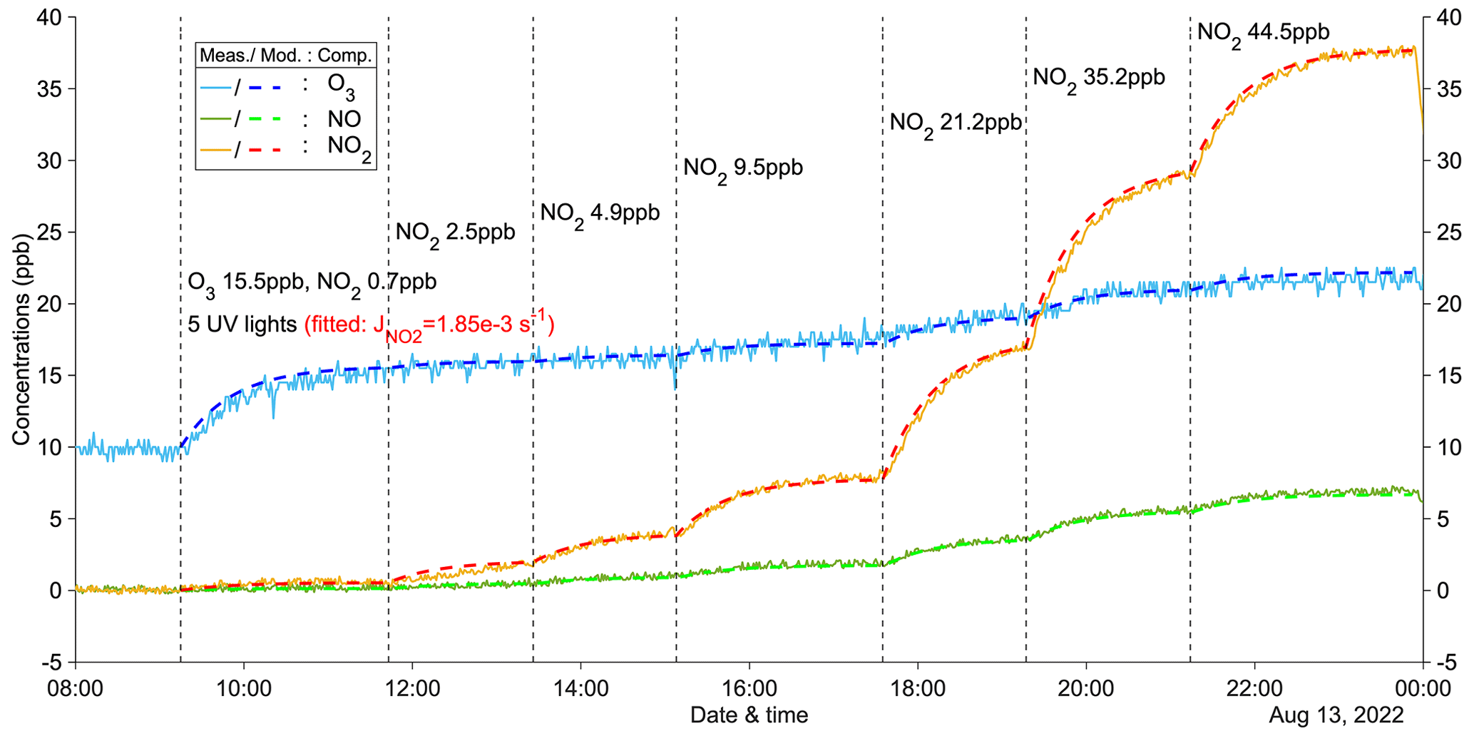
Figure A2A zero-VOC experiment (Z2) for determining the photolysis rate of NO2. Measured (abbreviated as Meas.) and modeled (abbreviated as Mod.) concentrations of different compounds (abbreviated as Comp.) are shown as solid and dashed lines, respectively. Dashed vertical lines indicate specific time points of operations, with corresponding labels for each operation.
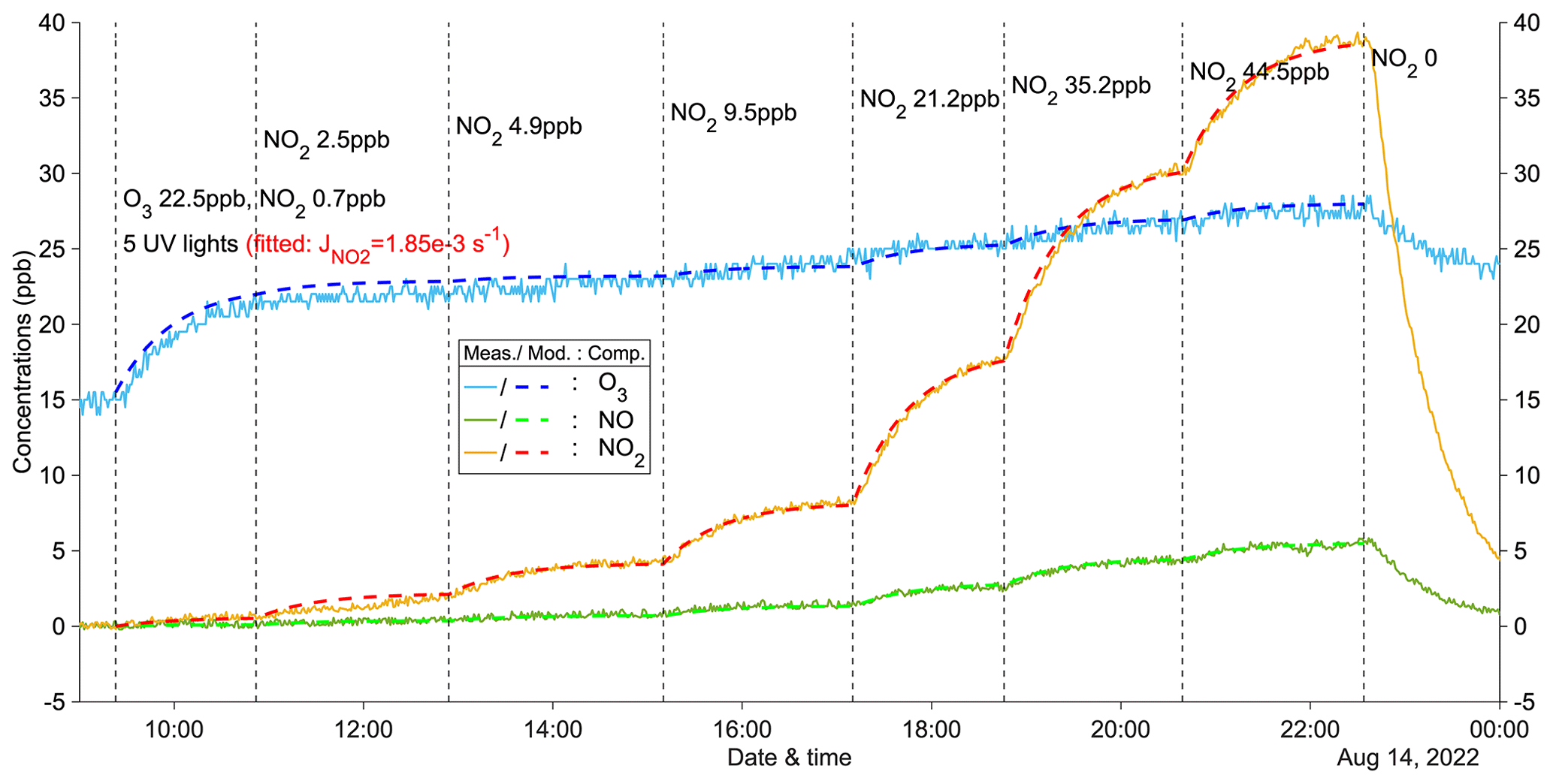
Figure A3A zero-VOC experiment (Z3) for determining the photolysis rate of NO2. Measured (abbreviated as Meas.) and modeled (abbreviated as Mod.) concentrations of different compounds (abbreviated as Comp.) are shown as solid and dashed lines, respectively. Dashed vertical lines indicate specific time points of operations, with corresponding labels for each operation.
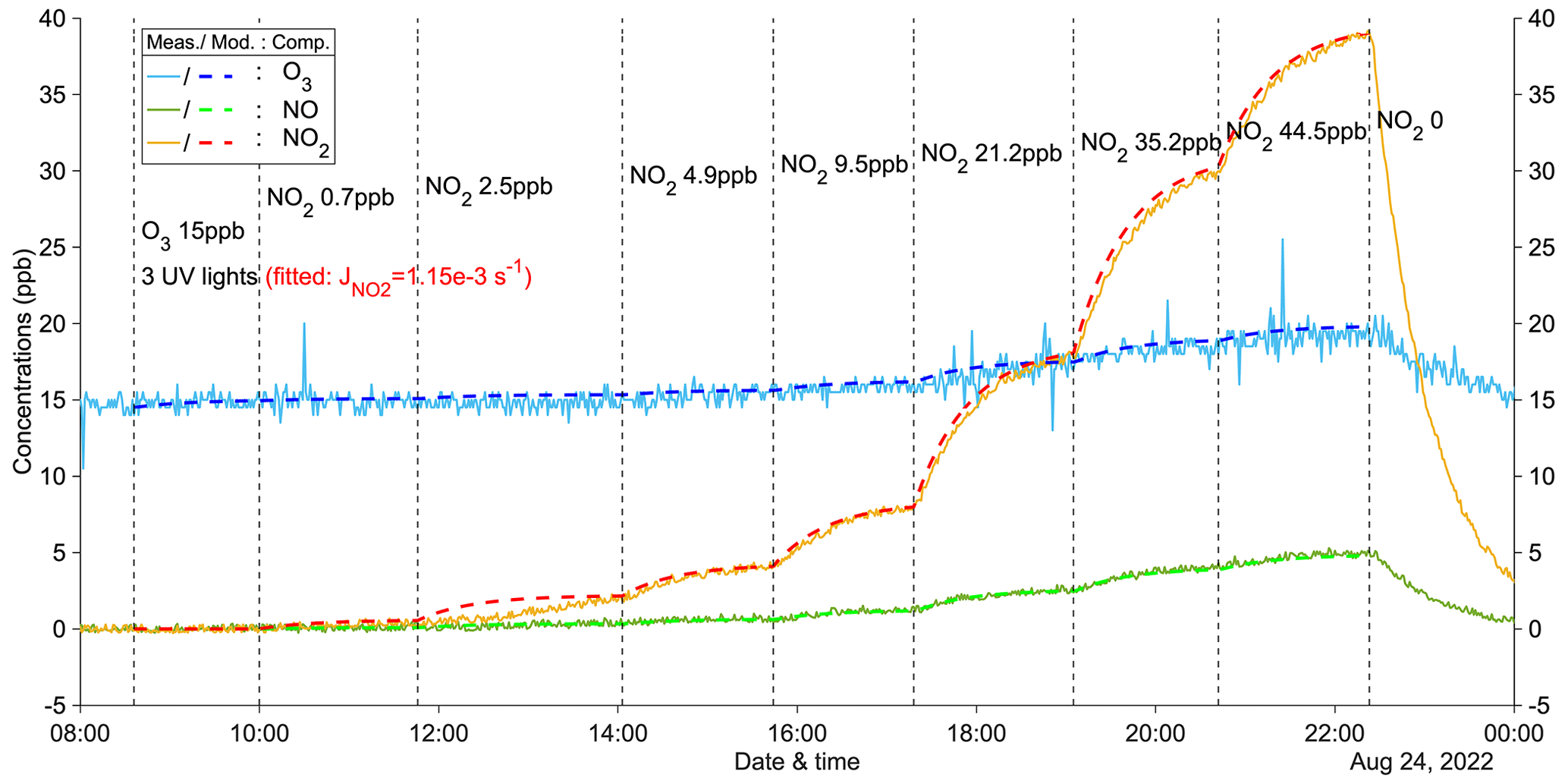
Figure A4A zero-VOC experiment (Z4) for determining the photolysis rate of NO2. Measured (abbreviated as Meas.) and modeled (abbreviated as Mod.) concentrations of different compounds (abbreviated as Comp.) are shown as solid and dashed lines, respectively. Dashed vertical lines indicate specific time points of operations, with corresponding labels for each operation.
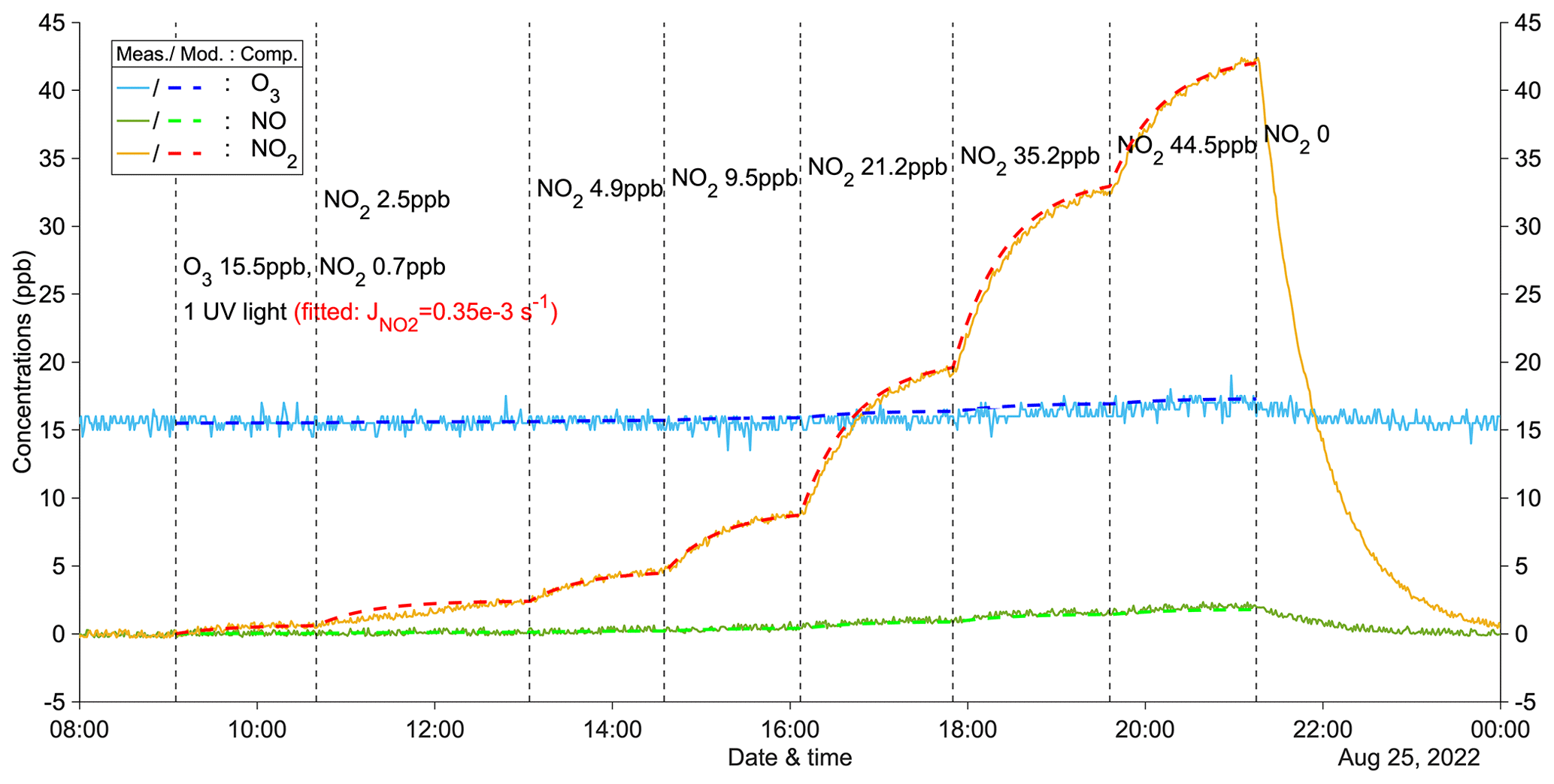
Figure A5A zero-VOC experiment (Z5) for determining the photolysis rate of NO2. Measured (abbreviated as Meas.) and modeled (abbreviated as Mod.) concentrations of different compounds (abbreviated as Comp.) are shown as solid and dashed lines, respectively. Dashed vertical lines indicate specific time points of operations, with corresponding labels for each operation.
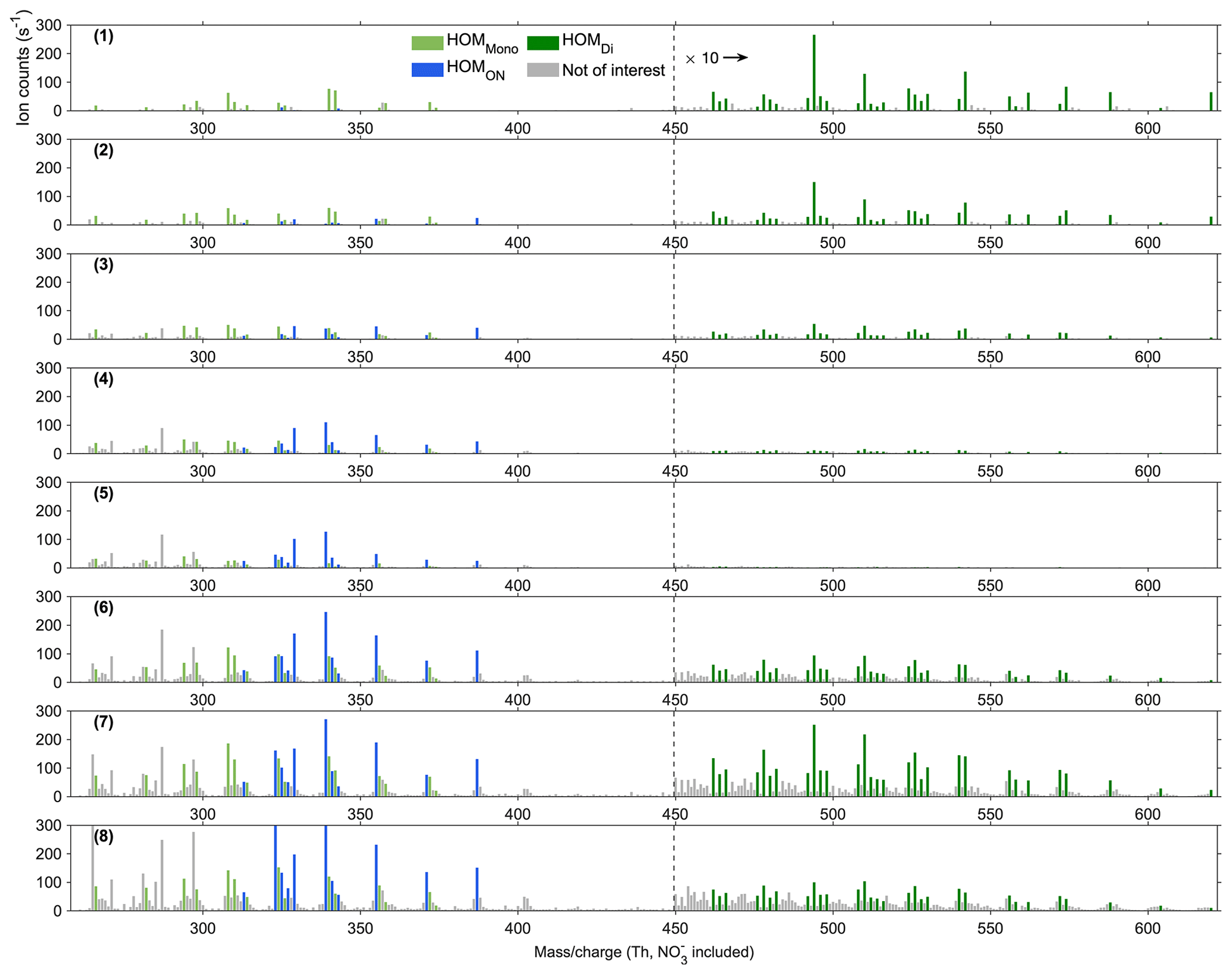
Figure A6Steady-state spectra (15 min average) for experiment no. 2 from the NO3-CIMS. All spectra were corrected by subtracting the corresponding background signals. The number in each row shows the order of the stage, consistent with the time series in Fig. 4. Light green bars show HOMMono, dark green ones show HOMDi, blue ones show HOMON, and grey ones show peaks not of interest. The peaks larger than 450 Th are multiplied by 10.
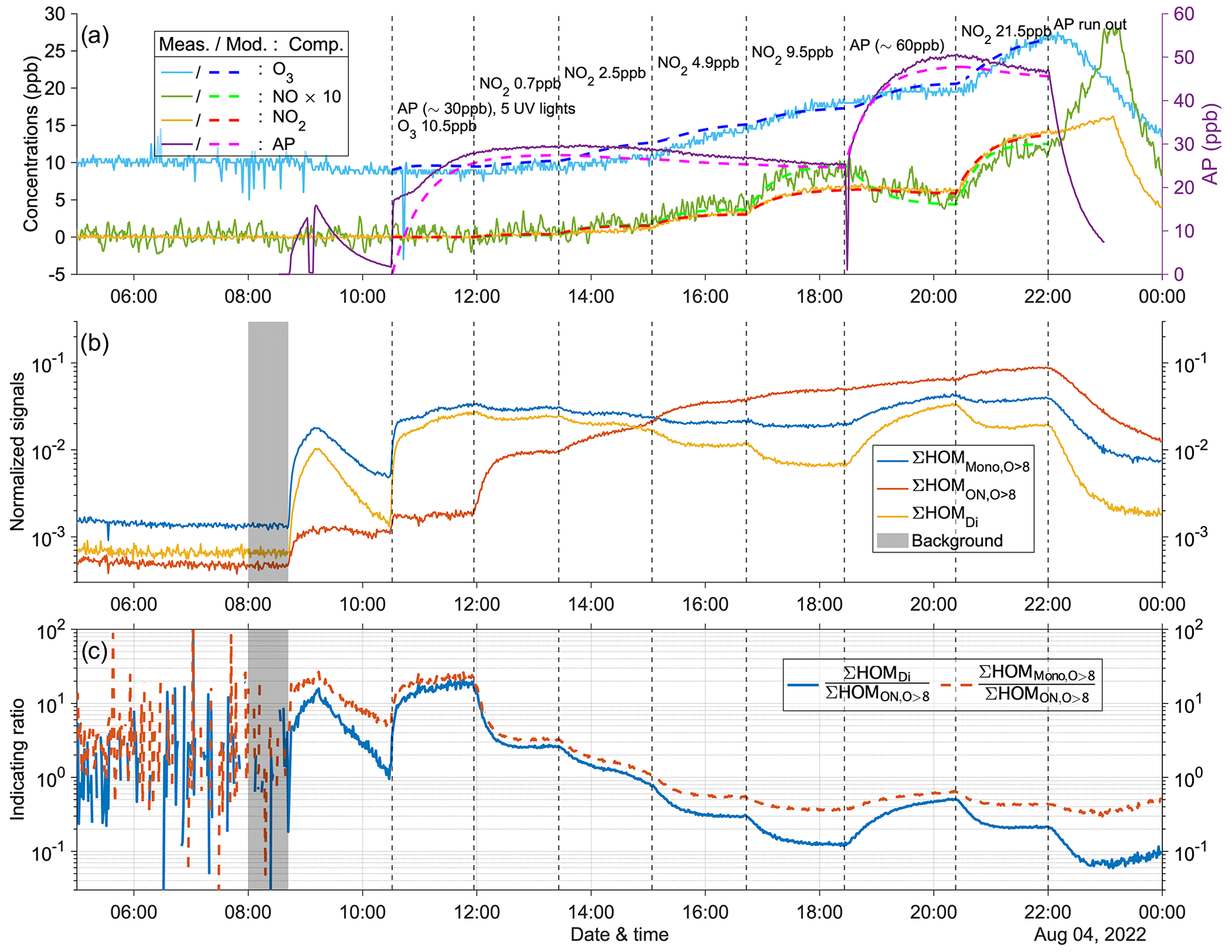
Figure A7Time series of experiment no. 1 with 30 ppb α-pinene and 10.5 ppb O3 as initial inputs. Five UV lights were on during all stages. Three panels show the time series of different compounds: (a) measured (abbreviated as Meas., solid lines) and modeled (abbreviated as Mod., dashed lines) concentrations of O3, NOx (both shown by the left y axis; the NO concentration is multiplied by 10), and AP (i.e., α-pinene, shown by the right y axis); (b) normalized signals of ∑HOM (sum of non-nitrate HOM monomers with more than eight oxygen atoms), ∑ HOM (sum of HOM organic nitrates with more than eight oxygen atoms), and ∑HOMDi (sum of HOM dimers); (c) IR1 and IR2 . The grey shaded area represents the time period selected for background subtraction before calculating the ratio. Dashed vertical lines indicate specific time points of operations, with the corresponding labels for each operation in panel (a).
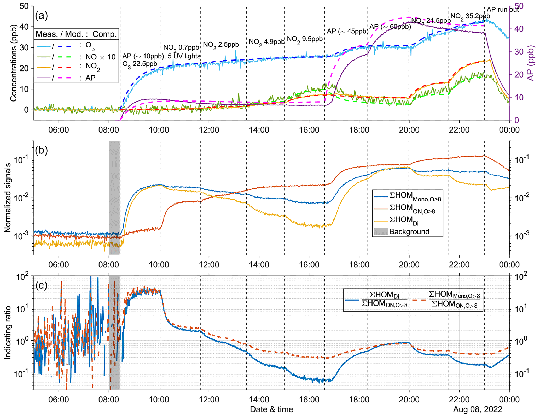
Figure A8Time series of experiment no. 3 with 10 ppb α-pinene and 22.5 ppb O3 as initial inputs. Five UV lights were on during all stages. Three panels show the time series of different compounds: (a) measured (abbreviated as Meas., solid lines) and modeled (abbreviated as Mod., dashed lines) concentrations of O3, NOx (both shown by the left y axis; the NO concentration is multiplied by 10), and AP (i.e., α-pinene, shown by the right y axis); (b) normalized signals of ∑HOM (sum of non-nitrate HOM monomers with more than eight oxygen atoms), ∑ HOM (sum of HOM organic nitrates with more than eight oxygen atoms), and ∑HOMDi (sum of HOM dimers); (c) IR1 and IR2 . The grey shaded area represents the time period selected for background subtraction before calculating the ratio. Dashed vertical lines indicate specific time points of operations, with the corresponding labels for each operation in panel (a).
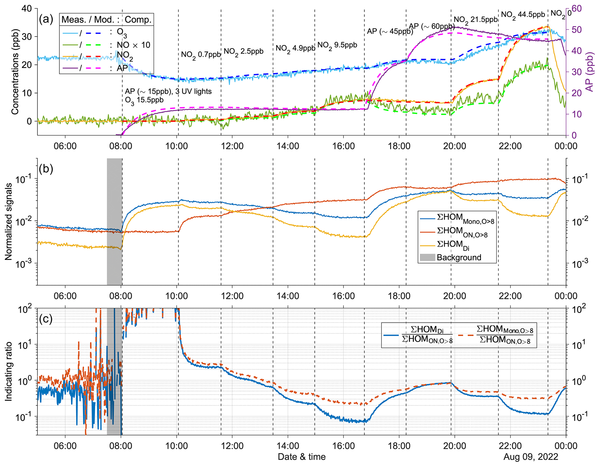
Figure A9Time series of experiment no. 4 with 15 ppb α-pinene and 15.5 ppb O3 as initial inputs. Three UV lights were on during all stages. Three panels show the time series of different compounds: (a) measured (abbreviated as Meas., solid lines) and modeled (abbreviated as Mod., dashed lines) concentrations of O3, NOx (both shown by the left y axis; the NO concentration is multiplied by 10), and AP (i.e., α-pinene, shown by the right y axis); (b) normalized signals of ∑HOM (sum of non-nitrate HOM monomers with more than eight oxygen atoms), ∑ HOM (sum of HOM organic nitrates with more than eight oxygen atoms), and ∑HOMDi (sum of HOM dimers); (c) IR1 and IR2 . The grey shaded area represents the time period selected for background subtraction before calculating the ratio. Dashed vertical lines indicate specific time points of operations, with the corresponding labels for each operation in panel (a).
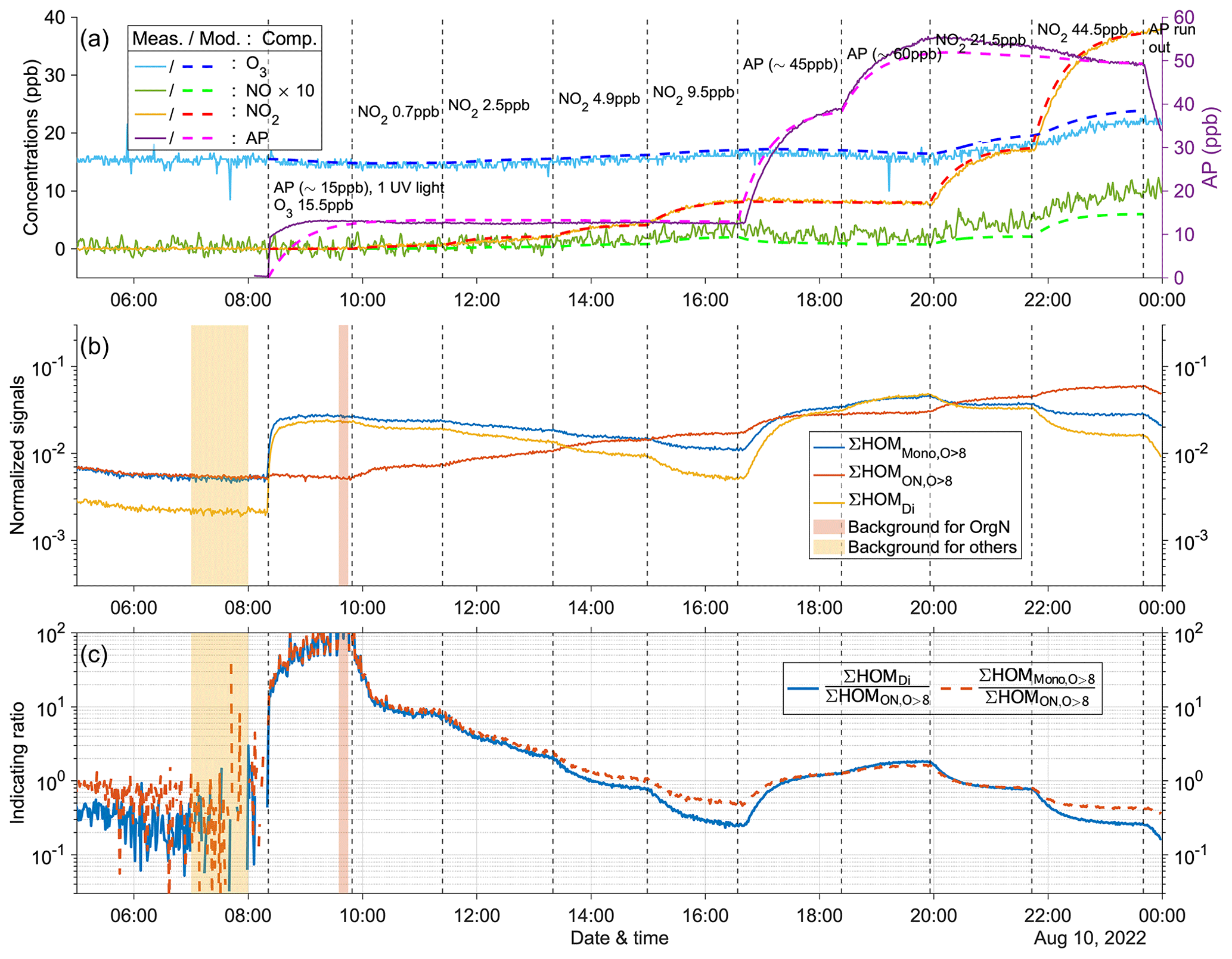
Figure A10Time series of experiment no. 5 with 15 ppb α-pinene and 15.5 ppb O3 as initial inputs. One UV light was on during all stages. Three panels show the time series of different compounds: (a) measured (abbreviated as Meas., solid lines) and modeled (abbreviated as Mod., dashed lines) concentrations of O3, NOx (both shown by the left y axis; the NO concentration is multiplied by 10), and AP (i.e., α-pinene, shown by the right y axis); (b) normalized signals of ∑HOM (sum of non-nitrate HOM monomers with more than eight oxygen atoms), ∑ HOM (sum of HOM organic nitrates with more than eight oxygen atoms), and ∑HOMDi (sum of HOM dimers); (c) IR1 and IR2 . The yellow and red shaded areas represent the time periods selected for background subtraction of dimers and organic nitrates before calculating the ratio. Dashed vertical lines indicate specific time points of operations, with the corresponding labels for each operation in panel (a).
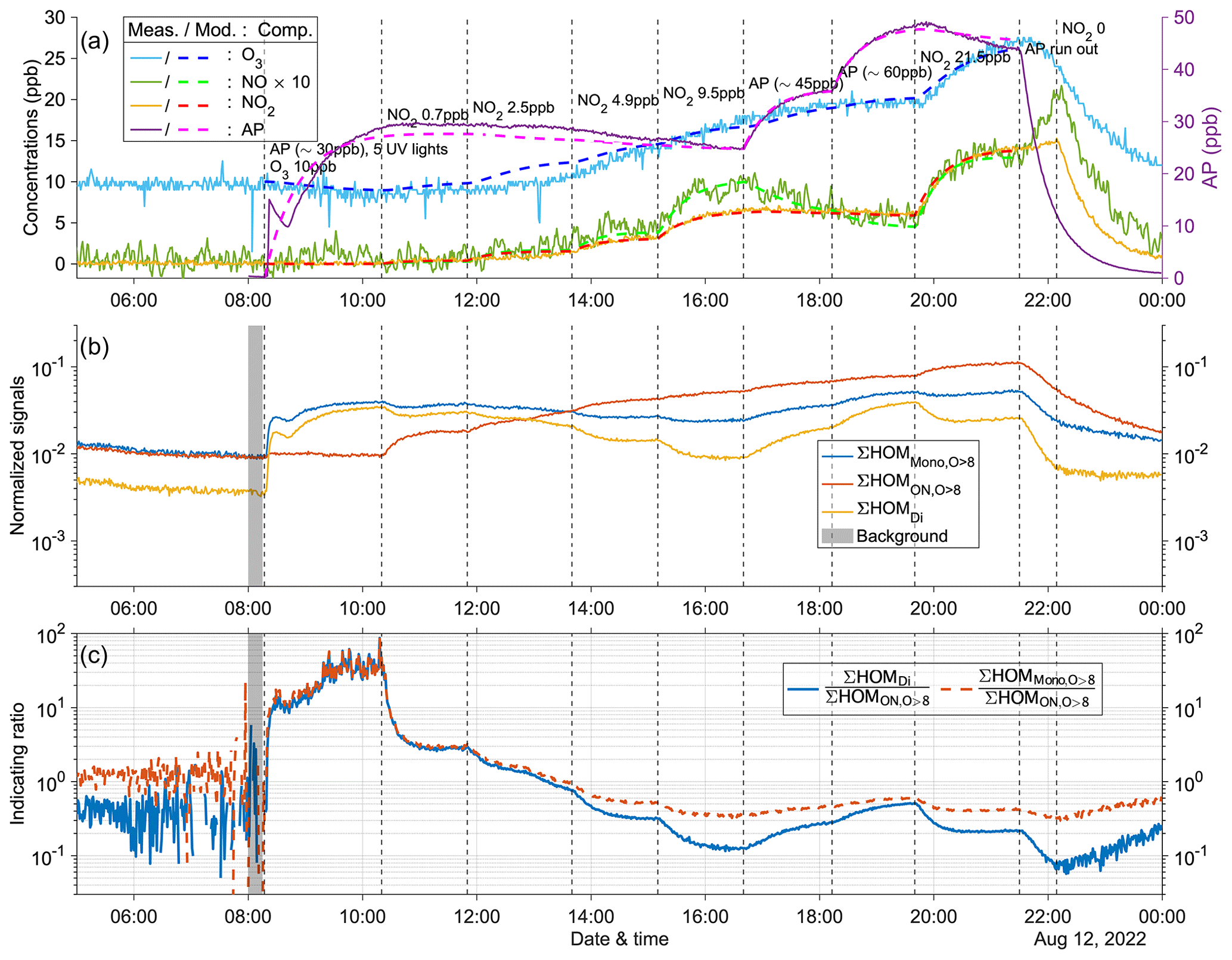
Figure A11Time series of experiment no. 7 with 30 ppb α-pinene and 10 ppb O3 as initial inputs. Five UV lights were on during all stages. Three panels show the time series of different compounds: (a) measured (abbreviated as Meas., solid lines) and modeled (abbreviated as Mod., dashed lines) concentrations of O3, NOx (both shown by the left y axis; the NO concentration is multiplied by 10), and AP (i.e., α-pinene, shown by the right y axis); (b) normalized signals of ∑HOM (sum of non-nitrate HOM monomers with more than eight oxygen atoms), ∑ HOM (sum of HOM organic nitrates with more than eight oxygen atoms), and ∑HOMDi (sum of HOM dimers); (c) IR1 and IR2 . The grey shaded area represents the time period selected for background subtraction before calculating the ratio. Dashed vertical lines indicate specific time points of operations, with the corresponding labels for each operation in panel (a).
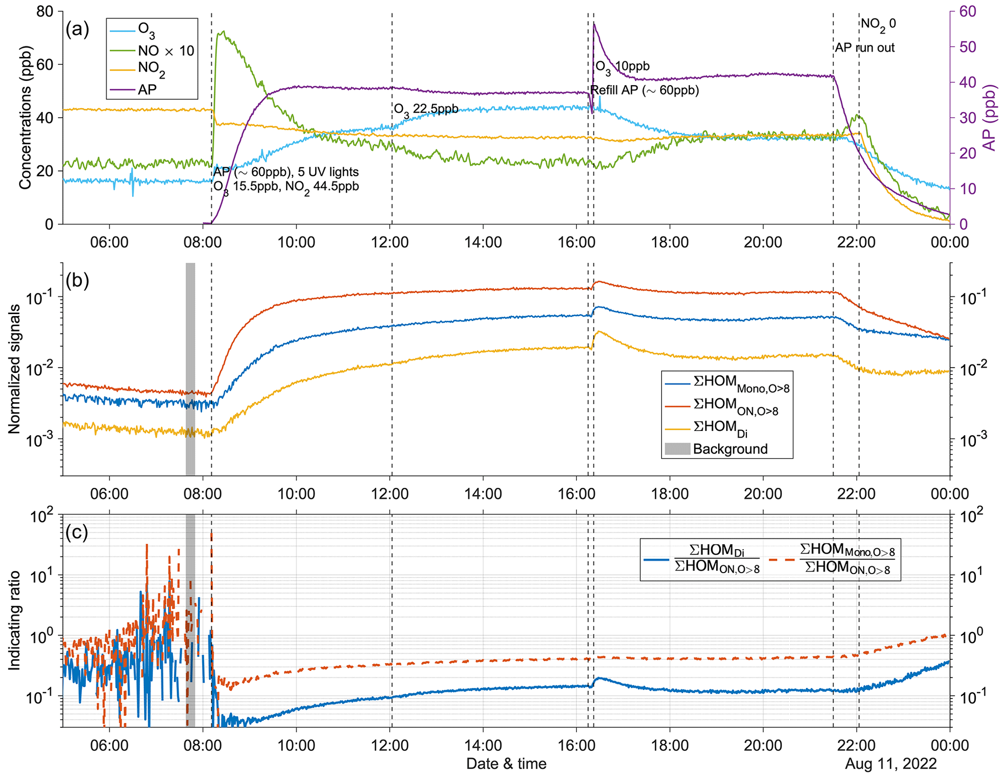
Figure A12Time series of experiment no. 6, which was meant for collecting more data at the highest NO2 input (at ∼ 44.5 ppb). Five UV lights were on during all stages. Three panels show the time series of different compounds: (a) measured concentrations of O3, NOx (both shown by the left y axis; the NO concentration is multiplied by 10), and AP (i.e., α-pinene, shown by the right y axis); (b) normalized signals of ∑HOM (sum of non-nitrate HOM monomers with more than eight oxygen atoms), ∑ HOM (sum of HOM organic nitrates with more than eight oxygen atoms), and ∑HOMDi (sum of HOM dimers); (c) IR1 and IR2 . The grey shaded area represents the time period selected for background subtraction before calculating the ratio. Dashed vertical lines indicate specific time points of operations, with the corresponding labels for each operation in panel (a).
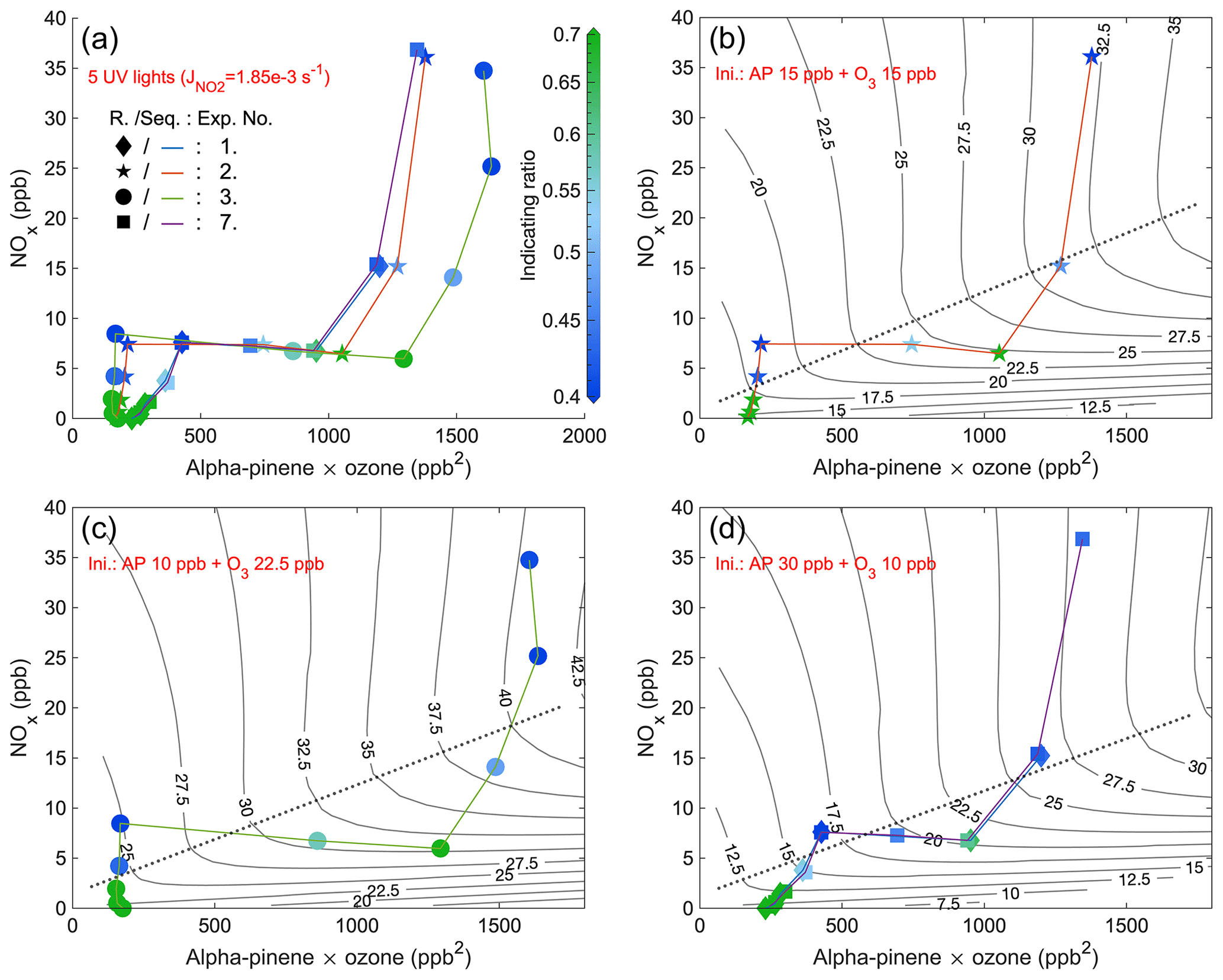
Figure A13Steady-state IR2 of experiments from 4 d with five UV lights. The x axis is the multiplication of steady-state α-pinene and O3 concentrations, while the y axis is the steady-state NOx. The scatter points (exp. no. 1: diamond; exp. no. 2: star; exp. no. 3: round; exp. no. 7: square) are colored by values of IR2 (abbreviated as R. in the figure) and are connected by curves (exp. no. 1: blue; exp. no. 2: orange; exp. no. 3: green; exp. no. 7: purple) showing the sequence (Seq.) of experimental stages. Panel (a) combines stages of all 4 d, and the other three panels respectively show the stages of experiments with different initial (Ini.) inputs (exp. nos. 1 and 7 are in the same panel (d) due to the same initial inputs). EKMA curves (isopleths of O3 concentrations in ppb), simulated by the box model, are solid black lines, while dotted lines are the corresponding ridge lines.
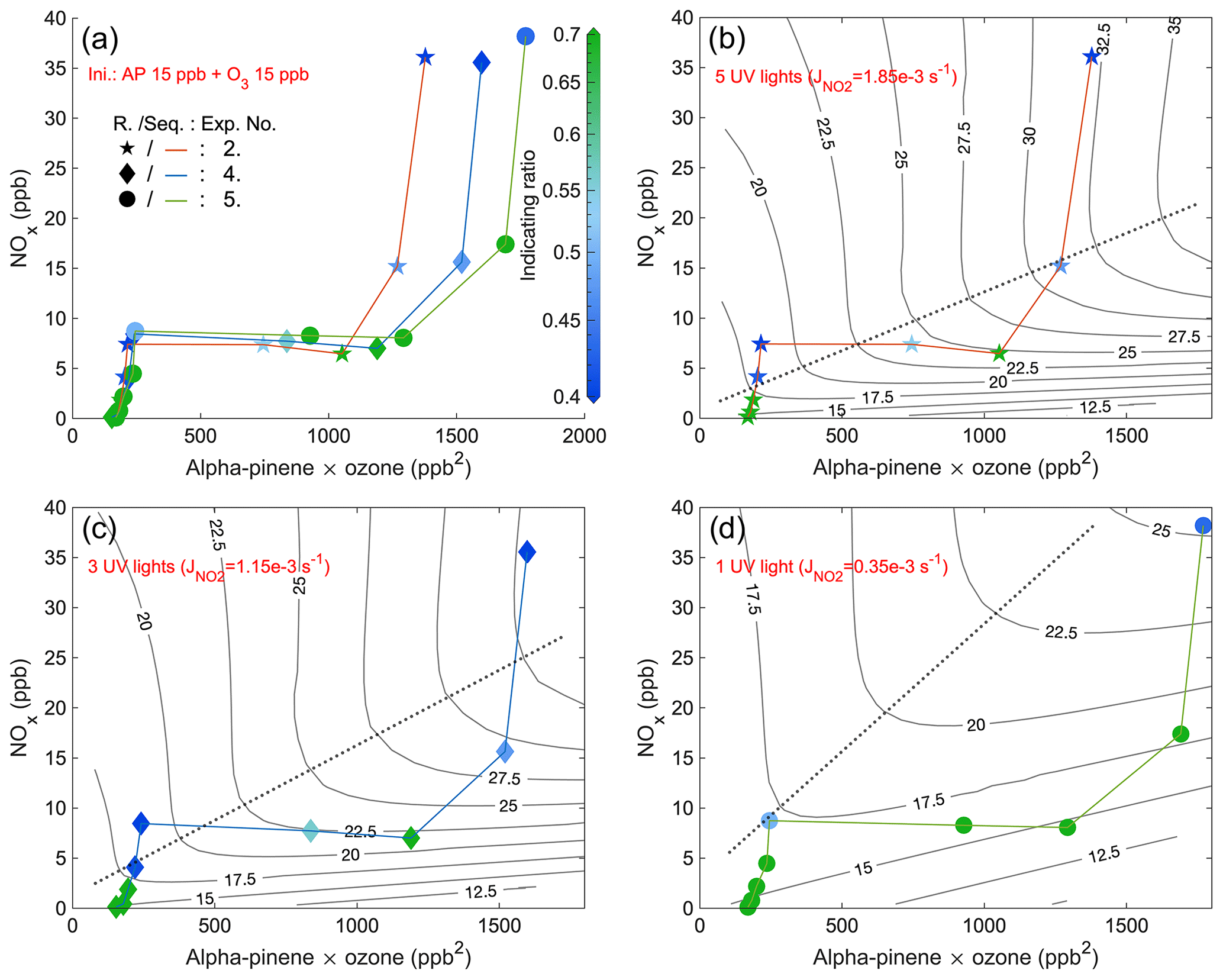
Figure A14Steady-state IR2 of experiments from 3 day with five UV lights, three UV lights, and one UV light, respectively. The x axis is the multiplication of steady-state α-pinene and O3 concentrations, while the y axis is the steady-state NOx. The scatter points (exp. no. 2: star; exp. no. 4: diamond; exp. no. 5: round) are colored by values of IR2 (abbreviated as R. in the figure) and are connected by curves (exp. no. 2: orange; exp. no. 4: blue; exp. no. 5: green) showing the sequence (Seq.) of experimental stages. Panel (a) combines stages of all 3 d with the same initial (Ini.) inputs, and the other three panels respectively show the stages of experiments with different numbers of UV lights. EKMA curves by the box model are black lines and the dotted lines are the corresponding ridge lines.
Table A1Zero-VOC experiment conditions. The experiment number (no.) and number of total stages are shown in the first two columns. Input information includes the number and NO2 photolysis rates () of UV lights (λ≈ 400 nm) as well as concentrations of O3, α-pinene, and NOx.
From the steady-state (ss in subscript) balance of the O3 concentration, we can write the following expression:
where is the residence time. O3 has NO2 photolysis and its input as sources, with reaction to NO and flush-out as sinks. We can solve the equation to get the NO2 photolysis rate.
This expression can be used for each steady state to estimate in the corresponding experiment.
Table A2Reactions and their reaction rate coefficients used for the box model. Note that RO2 represents all kinds of peroxy radicals, and thus there are huge uncertainties regarding reaction rates. This model is only meant for simulating concentrations of O3 and its precursors.
a Except the NO2 photolysis and wall loss rates (s−1), all the other reaction rates (cm3 s−1) are adapted from the NIST (National Institute of Standards and Technology) Chemical Kinetics Database (for more information see https://kinetics.nist.gov/kinetics/index.jsp (last access: 25 August 2023). b In our model, we only considered RO2 with a wall loss lifetime of 400 s (Peräkylä et al., 2020).
Code is available upon request from the corresponding authors.
Data are available upon request from the corresponding authors.
ME, JZ, and JYZ designed the study. JZ, JYZ, YL, and VM conducted the experiments. JYZ analyzed the data and developed the model. ME, JZ, and DR supported the data analysis.
The contact author has declared that none of the authors has any competing interests.
Publisher's note: Copernicus Publications remains neutral with regard to jurisdictional claims made in the text, published maps, institutional affiliations, or any other geographical representation in this paper. While Copernicus Publications makes every effort to include appropriate place names, the final responsibility lies with the authors.
The authors thank Lauriane Quéléver for the calibration of the NO3-CIMS.
This research has been supported by the Academy of Finland (grant no. 345982) and the Jane ja Aatos Erkon Säätiö (the Jane and Aatos Erkko Foundation).
Open-access funding was provided by the Helsinki University Library.
This paper was edited by Markus Ammann and reviewed by two anonymous referees.
Archer, S. L., Shultz, P. J., Warren, J. B., Hampl, V., and DeMaster, E. G.: Preparation of standards and measurement of nitric oxide, nitroxyl, and related oxidation products, Methods, 7, 21–34, https://doi.org/10.1006/meth.1995.1004, 1995. a
Atkinson, R. and Arey, J.: Atmospheric degradation of volatile organic compounds, Chem. Rev., 103, 4605–4638, https://doi.org/10.1021/cr0206420, 2003. a, b
Atkinson, R., Baulch, D. L., Cox, R. A., Crowley, J. N., Hampson, R. F., Hynes, R. G., Jenkin, M. E., Rossi, M. J., and Troe, J.: Evaluated kinetic and photochemical data for atmospheric chemistry: Volume I - gas phase reactions of Ox, HOx, NOx and SOx species, Atmos. Chem. Phys., 4, 1461–1738, https://doi.org/10.5194/acp-4-1461-2004, 2004. a
Bianchi, F., Kurtén, T., Riva, M., Mohr, C., Rissanen, M. P., Roldin, P., Berndt, T., Crounse, J. D., Wennberg, P. O., Mentel, T. F., Wildt, J., Junninen, H., Jokinen, T., Kulmala, M., Worsnop, D. R., Thornton, J. A., Donahue, N., Kjaergaard, H. G., and Ehn, M.: Highly oxygenated organic molecules (HOM) from gas-phase autoxidation involving peroxy radicals: A key contributor to atmospheric aerosol, Chem. Rev., 119, 3472–3509, https://doi.org/10.1021/acs.chemrev.8b00395, 2019. a, b, c
Boucher, O., Randall, D., Artaxo, P., Bretherton, C., Feingold, G., Forster, P., Kerminen, V.-M., Kondo, Y., Liao, H., Lohmann, U., Rasch, P., Satheesh, S. K., Sherwood, S., Stevens, B., and Zhang, X. Y.: Clouds and aerosols, in: Climate change 2013: The physical science basis. Contribution of working group I to the fifth assessment report of the intergovernmental panel on climate change, Cambridge University Press, Cambridge, 571–657, 571–657, https://doi.org/10.1017/CBO9781107415324.016, 2013. a
Chameides, W. L., Fehsenfeld, F., Rodgers, M. O., Cardelino, C., Martinez, J., Parrish, D., Lonneman, W., Lawson, D. R., Rasmussen, R. A., Zimmerman, P., Greenberg, J., Mlddleton, P., and Wang, T.: Ozone precursor relationships in the ambient atmosphere, J. Geophys. Res.-Atmos., 97, 6037–6055, https://doi.org/10.1029/91JD03014, 1992. a
Chapman, S.: A theory of upper-atmospheric ozone, Mem. R. Metrol. Soc., 3, 103–125, https://cir.nii.ac.jp/crid/1572261549196038528 (last access: 1 August 2023), 1930. a, b
Chipperfield, M. P., Bekki, S., Dhomse, S., Harris, N. R. P., Hassler, B., Hossaini, R., Steinbrecht, W., Thiéblemont, R., and Weber, M.: Detecting recovery of the stratospheric ozone layer, Nature, 549, 211–218, https://doi.org/10.1038/nature23681, 2017. a
Crounse, J. D., Nielsen, L. B., Jørgensen, S., Kjaergaard, H. G., and Wennberg, P. O.: Autoxidation of organic compounds in the atmosphere, J. Phys. Chem. Lett., 4, 3513–3520, https://doi.org/10.1021/jz4019207, 2013. a
Crutzen, P. J.: The influence of nitrogen oxides on the atmospheric ozone content, Q. J. Roy. Meteor. Soc., 96, 320–325, https://doi.org/10.1002/qj.49709640815, 1970. a
Crutzen, P. J.: Ozone production rates in an oxygen-hydrogen-nitrogen oxide atmosphere, J. Geophys. Res., 76, 7311–7327, https://doi.org/10.1029/JC076i030p07311, 1971. a
Dickerson, R. R., Kondragunta, S., Stenchikov, G., Civerolo, K. L., Doddridge, B. G., and Holben, B. N.: The impact of aerosols on solar ultraviolet radiation and photochemical smog, Science, 278, 827–830, https://doi.org/10.1126/science.278.5339.827, 1997. a
Dodge, M. C.: Combined use of modeling techniques and smog chamber data to derive ozone-precursor relationships, in: International conference on photochemical oxidant pollution and its control: Proceedings,Environmental Sciences Research Laboratory Research Triangle Park, NC, 12–17 September 1976, US Environmental Protection Agency, 2, 881–889, 1977. a, b
Ehhalt, D., Prather, M., Dentener, F., Derwent, R., Dlugokencky, E., Holland, E., Isaksen, I., Katima, J., Kirchhoff, V., Matson, P., Midgley, P., and Wang, M.: Atmospheric chemistry and greenhouse gases, in: Climate Change 2001: the scientific basis, Intergovernmental panel on climate change, 2001, Cambridge University Press, Cambridge, https://hal.science/hal-03333922 (last access: 1 August 2023), 2001. a
Ehn, M., Thornton, J. A., Kleist, E., Sipilä, M., Junninen, H., Pullinen, I., Springer, M., Rubach, F., Tillmann, R., Lee, B., Lopez-Hilfiker, F., Andres, S., Acir, I.-H., Rissanen, M., Jokinen, T., Schobesberger, S., Kangasluoma, J., Kontkanen, J., Nieminen, T., Kurtén, T., Nielsen, L. B., Jørgensen, S., Kjaergaard, H. G., Canagaratna, M., Maso, M. D., Berndt, T., Petäjä, T., Wahner, A., Kerminen, V.-M., Kulmala, M., Worsnop, D. R., Wildt, J., and Mentel, T. F.: A large source of low-volatility secondary organic aerosol, Nature, 506, 476–479, https://doi.org/10.1038/nature13032, 2014. a, b, c
Graus, M., Müller, M., and Hansel, A.: High resolution PTR-TOF: Quantification and formula confirmation of VOC in real time, J. Am. Soc. Mass Spectr.., 21, 1037–1044, https://doi.org/10.1016/j.jasms.2010.02.006, 2010. a, b
Gruijl, F. d. and Leun, J.: Environment and health: 3. Ozone depletion and ultraviolet radiation, Can Med. Assoc. J., 163, 851–855, https://www.cmaj.ca/content/163/7/851 (last access: 1 August 2023), 2000. a
Haagen-Smit, A. J., Bradley, C. E., and Fox, M. M.: Ozone formation in photochemical oxidation of organic substances, Ind. Eng. Chem., 45, 2086–2089, https://doi.org/10.1021/ie50525a044, 1953. a
Hammer, M.-U., Vogel, B., and Vogel, H.: Findings on as an indicator of ozone sensitivity in Baden-Württemberg, Berlin-Brandenburg, and the Po valley based on numerical simulations, J. Geophys. Res.-Atmos., 107, 8190, https://doi.org/10.1029/2000JD000211, 2002. a
Hansel, A., Jordan, A., Holzinger, R., Prazeller, P., Vogel, W., and Lindinger, W.: Proton transfer reaction mass spectrometry: on-line trace gas analysis at the ppb level, Int. J. Mass Spectrom., 149-150, 609–619, https://doi.org/10.1016/0168-1176(95)04294-U, 1995. a, b
Harris, G. W., Carter, W. P. L., Winer, A. M., Pitts, J. N., Platt, U., and Perner, D.: Observations of nitrous acid in the Los Angeles atmosphere and implications for predictions of ozone-precursor relationships, Environ. Sci. Technol., 16, 414–419, https://doi.org/10.1021/es00101a009, 1982. a
He, X.-C., Shen, J., Iyer, S., Juuti, P., Zhang, J., Koirala, M., Kytökari, M. M., Worsnop, D. R., Rissanen, M., Kulmala, M., Maier, N. M., Mikkilä, J., Sipilä, M., and Kangasluoma, J.: Characterisation of gaseous iodine species detection using the multi-scheme chemical ionisation inlet 2 with bromide and nitrate chemical ionisation methods, Atmos. Meas. Tech., 16, 4461–4487, https://doi.org/10.5194/amt-16-4461-2023, 2023. a
Jokinen, T., Sipilä, M., Junninen, H., Ehn, M., Lönn, G., Hakala, J., Petäjä, T., Mauldin III, R. L., Kulmala, M., and Worsnop, D. R.: Atmospheric sulphuric acid and neutral cluster measurements using CI-APi-TOF, Atmos. Chem. Phys., 12, 4117–4125, https://doi.org/10.5194/acp-12-4117-2012, 2012. a, b
Jordan, A., Haidacher, S., Hanel, G., Hartungen, E., Märk, L., Seehauser, H., Schottkowsky, R., Sulzer, P., and Märk, T. D.: A high resolution and high sensitivity proton-transfer-reaction time-of-flight mass spectrometer (PTR-TOF-MS), Int. J. Mass Spectrom., 286, 122–128, https://doi.org/10.1016/j.ijms.2009.07.005, 2009. a
Junninen, H., Ehn, M., Petäjä, T., Luosujärvi, L., Kotiaho, T., Kostiainen, R., Rohner, U., Gonin, M., Fuhrer, K., Kulmala, M., and Worsnop, D. R.: A high-resolution mass spectrometer to measure atmospheric ion composition, Atmos. Meas. Tech., 3, 1039–1053, https://doi.org/10.5194/amt-3-1039-2010, 2010. a, b
Kelly, F. J. and Fussell, J. C.: Air pollution and public health: emerging hazards and improved understanding of risk, Environ. Geochem. Hlth., 37, 631–649, https://doi.org/10.1007/s10653-015-9720-1, 2015. a
Kinosian, J. R.: Ozone-precursor relationships from EKMA diagrams, Environ. Sci. Technol., 16, 880–883, https://doi.org/10.1021/es00106a011, 1982. a, b
Kleinman, L. I., Daum, P. H., Lee, Y.-N., Nunnermacker, L. J., Springston, S. R., Weinstein-Lloyd, J., and Rudolph, J.: Ozone production efficiency in an urban area, J. Geophys. Res.-Atmos., 107, 4733, https://doi.org/10.1029/2002JD002529, 2002. a
Krechmer, J. E., Day, D. A., and Jimenez, J. L.: Always lost but never forgotten: Gas-phase wall losses are important in all teflon nnvironmental chambers, Environ. Sci. Technol., 54, 12890–12897, https://doi.org/10.1021/acs.est.0c03381, 2020. a
Kürten, A., Rondo, L., Ehrhart, S., and Curtius, J.: Calibration of a chemical ionization mass spectrometer for the measurement of gaseous sulfuric acid, J. Phys. Chem. A, 116, 6375–6386, https://doi.org/10.1021/jp212123n, 2012. a
Kürten, A., Jokinen, T., Simon, M., Sipilä, M., Sarnela, N., Junninen, H., Adamov, A., Almeida, J., Amorim, A., Bianchi, F., Breitenlechner, M., Dommen, J., Donahue, N. M., Duplissy, J., Ehrhart, S., Flagan, R. C., Franchin, A., Hakala, J., Hansel, A., Heinritzi, M., Hutterli, M., Kangasluoma, J., Kirkby, J., Laaksonen, A., Lehtipalo, K., Leiminger, M., Makhmutov, V., Mathot, S., Onnela, A., Petäjä, T., Praplan, A. P., Riccobono, F., Rissanen, M. P., Rondo, L., Schobesberger, S., Seinfeld, J. H., Steiner, G., Tomé, A., Tröstl, J., Winkler, P. M., Williamson, C., Wimmer, D., Ye, P., Baltensperger, U., Carslaw, K. S., Kulmala, M., Worsnop, D. R., and Curtius, J.: Neutral molecular cluster formation of sulfuric acid–dimethylamine observed in real time under atmospheric conditions, P. Natl. Acad. Sci. USA, 111, 15019–15024, https://doi.org/10.1073/pnas.1404853111, 2014. a
Lelieveld, J. and Dentener, F.: What controls tropospheric ozone?, J. Geophys. Res.-Atmos., 105, 3531–3551, https://doi.org/10.1029/1999JD901011, 2000. a
Liu, C. and Shi, K.: A review on methodology in O3-NOx-VOC sensitivity study, Environ. Pollut., 291, 118249, https://doi.org/10.1016/j.envpol.2021.118249, 2021. a, b, c
Madronich, S., Hastie, D. R., Ridley, B. A., and Schiff, H. I.: Measurement of the photodissociation coefficient of NO2 in the atmosphere. I – Method and surface measurements, J. Atmos. Chem., 1, 3–25, https://doi.org/10.1007/BF00113977, 1983. a
Martin, R., Fiore, A., and Donkelaar, A.: Space-based diagnosis of surface ozone sensitivity to anthropogenic emissions, Geophys. Res. Lett, 31, L06120, https://doi.org/10.1029/2004GL019416, 2004. a
Melkonyan, A. and Kuttler, W.: Long-term analysis of NO, NO2 and O3 concentrations in North Rhine-Westphalia, Germany, Atmos. Environ., 60, 316–326, https://doi.org/10.1016/j.atmosenv.2012.06.048, 2012. a
Meyer Jr, E. L., Summerhays, J. P., and Freas, W.: Uses, limitations, and technical basis of procedures for quantifying relationships between photochemical oxidants and precursors, in: EPA-450/2-77-021a, Environmental Protection Agency Research, Triangle Park, NC, 1977. a
Nuvolone, D., Petri, D., and Voller, F.: The effects of ozone on human health, Environ. Sci. Pollut. R., 25, 8074–8088, https://doi.org/10.1007/s11356-017-9239-3, 2018. a, b
Pathak, R. K., Stanier, C. O., Donahue, N. M., and Pandis, S. N.: Ozonolysis of α-pinene at atmospherically relevant concentrations: Temperature dependence of aerosol mass fractions (yields), J. Geophys. Res.-Atmos., 112, D03201, https://doi.org/10.1029/2006JD007436, 2007. a
Peräkylä, O., Riva, M., Heikkinen, L., Quéléver, L., Roldin, P., and Ehn, M.: Experimental investigation into the volatilities of highly oxygenated organic molecules (HOMs) , Atmos. Chem. Phys., 20, 649–669, https://doi.org/10.5194/acp-20-649-2020, 2020. a, b
Riva, M., Heikkinen, L., Bell, D. M., Peräkylä, O., Zha, Q., Schallhart, S., Rissanen, M. P., Imre, D., Petäjä, T., Thornton, J. A., Zelenyuk, A., and Ehn, M.: Chemical transformations in monoterpene-derived organic aerosol enhanced by inorganic composition, npj Climate and Atmospheric Science, 2, 1–9, https://doi.org/10.1038/s41612-018-0058-0, 2019a. a, b
Riva, M., Rantala, P., Krechmer, J. E., Peräkylä, O., Zhang, Y., Heikkinen, L., Garmash, O., Yan, C., Kulmala, M., Worsnop, D., and Ehn, M.: Evaluating the performance of five different chemical ionization techniques for detecting gaseous oxygenated organic species, Atmos. Meas. Tech., 12, 2403–2421, https://doi.org/10.5194/amt-12-2403-2019, 2019b. a
Sandermann, H.: Ozone and plant health, Annu. Rev. Phytopathol., 34, 347–366, https://doi.org/10.1146/annurev.phyto.34.1.347, 1996. a
Seinfeld, J. H. and Pandis, S. N.: Atmospheric chemistry and physics: From air pollution to climate change, John Wiley & Sons, Hoboken, ISBN: 978-1-118-94740-1, 2016. a, b, c
Seviour, W. J. M.: Good ozone, bad ozone and the Southern Ocean, Nat. Clim. Change, 12, 316–317, https://doi.org/10.1038/s41558-022-01322-8, 2022. a
Sicard, P., De Marco, A., Agathokleous, E., Feng, Z., Xu, X., Paoletti, E., Rodriguez, J. J. D., and Calatayud, V.: Amplified ozone pollution in cities during the COVID-19 lockdown, Sci. Total Environ., 735, 139542, https://doi.org/10.1016/j.scitotenv.2020.139542, 2020. a
Sillman, S.: The relation between ozone, NOx and hydrocarbons in urban and polluted rural environments, Atmos. Environ., 33, 1821–1845, https://doi.org/10.1016/S1352-2310(98)00345-8, 1999. a, b
Sillman, S., Logan, J. A., and Wofsy, S. C.: The sensitivity of ozone to nitrogen oxides and hydrocarbons in regional ozone episodes, J. Geophys. Res.-Atmos., 95, 1837–1851, https://doi.org/10.1029/JD095iD02p01837, 1990. a
Staehelin, J., Harris, N. R. P., Appenzeller, C., and Eberhard, J.: Ozone trends: A review, Rev. Geophys., 39, 231–290, https://doi.org/10.1029/1999RG000059, 2001. a
Stolarski, R. S. and Cicerone, R. J.: Stratospheric chlorine: a possible sink for ozone, Can. J. Chem., 52, 1610–1615, https://doi.org/10.1139/v74-233, 1974. a
Tang, X., Li, J., and Chen, D.: Summertime photochemical pollution in Beijing, Pure Appl. Chem., 67, 1465–1468, 1995. a
Tiao, G. C., Box, G. E. P., and Hamming, W. J.: Analysis of Los Angeles photochemical smog data: a statistical overview, JAPCA J. Air Waste Ma., 25, 260–268, https://doi.org/10.1080/00022470.1975.10470082, 1975. a, b
Trainer, M., Parrish, D. D., Buhr, M. P., Norton, R. B., Fehsenfeld, F. C., Anlauf, K. G., Bottenheim, J. W., Tang, Y. Z., Wiebe, H. A., Roberts, J. M., Tanner, R. L., Newman, L., Bowersox, V. C., Meagher, J. F., Olszyna, K. J., Rodgers, M. O., Wang, T., Berresheim, H., Demerjian, K. L., and Roychowdhury, U. K.: Correlation of ozone with NOy in photochemically aged air, J. Geophys. Res.-Atmos., 98, 2917–2925, https://doi.org/10.1029/92JD01910, 1993. a
Wang, T., Ding, A., Gao, J., and Wu, W. S.: Strong ozone production in urban plumes from Beijing, China, Geophys. Res. Lett., 33, L21806, https://doi.org/10.1029/2006GL027689, 2006. a
Wang, T., Xue, L., Brimblecombe, P., Lam, Y. F., Li, L., and Zhang, L.: Ozone pollution in China: A review of concentrations, meteorological influences, chemical precursors, and effects, Sci. Total Environ., 575, 1582–1596, https://doi.org/10.1016/j.scitotenv.2016.10.081, 2017. a, b, c
Yan, C., Nie, W., Äijälä, M., Rissanen, M. P., Canagaratna, M. R., Massoli, P., Junninen, H., Jokinen, T., Sarnela, N., Häme, S. A. K., Schobesberger, S., Canonaco, F., Yao, L., Prévôt, A. S. H., Petäjä, T., Kulmala, M., Sipilä, M., Worsnop, D. R., and Ehn, M.: Source characterization of highly oxidized multifunctional compounds in a boreal forest environment using positive matrix factorization, Atmos. Chem. Phys., 16, 12715–12731, https://doi.org/10.5194/acp-16-12715-2016, 2016. a
Yan, C., Nie, W., Vogel, A. L., Dada, L., Lehtipalo, K., Stolzenburg, D., Wagner, R., Rissanen, M. P., Xiao, M., Ahonen, L., Fischer, L., Rose, C., Bianchi, F., Gordon, H., Simon, M., Heinritzi, M., Garmash, O., Roldin, P., Dias, A., Ye, P., Hofbauer, V., Amorim, A., Bauer, P. S., Bergen, A., Bernhammer, A.-K., Breitenlechner, M., Brilke, S., Buchholz, A., Mazon, S. B., Canagaratna, M. R., Chen, X., Ding, A., Dommen, J., Draper, D. C., Duplissy, J., Frege, C., Heyn, C., Guida, R., Hakala, J., Heikkinen, L., Hoyle, C. R., Jokinen, T., Kangasluoma, J., Kirkby, J., Kontkanen, J., Kürten, A., Lawler, M. J., Mai, H., Mathot, S., Mauldin, R. L., Molteni, U., Nichman, L., Nieminen, T., Nowak, J., Ojdanic, A., Onnela, A., Pajunoja, A., Petäjä, T., Piel, F., Quéléver, L. L. J., Sarnela, N., Schallhart, S., Sengupta, K., Sipilä, M., Tomé, A., Tröstl, J., Väisänen, O., Wagner, A. C., Ylisirniö, A., Zha, Q., Baltensperger, U., Carslaw, K. S., Curtius, J., Flagan, R. C., Hansel, A., Riipinen, I., Smith, J. N., Virtanen, A., Winkler, P. M., Donahue, N. M., Kerminen, V.-M., Kulmala, M., Ehn, M., and Worsnop, D. R.: Size-dependent influence of NOx on the growth rates of organic aerosol particles, Science Advances, 6, eaay4945, https://doi.org/10.1126/sciadv.aay4945, 2020. a
Zhao, J., Häkkinen, E., Graeffe, F., Krechmer, J. E., Canagaratna, M. R., Worsnop, D. R., Kangasluoma, J., and Ehn, M.: A combined gas- and particle-phase analysis of highly oxygenated organic molecules (HOMs) from α-pinene ozonolysis, Atmos. Chem. Phys., 23, 3707–3730, https://doi.org/10.5194/acp-23-3707-2023, 2023a. a, b
Zhao, J., Mickwitz, V., Luo, Y., Häkkinen, E., Graeffe, F., Zhang, J., Timonen, H., Canagaratna, M., Krechmer, J. E., Zhang, Q., Kulmala, M., Kangasluoma, J., Worsnop, D., and Ehn, M.: Characterization of the Vaporization Inlet for Aerosols (VIA) for Online Measurements of Particulate Highly Oxygenated Organic Molecules (HOMs), EGUsphere [preprint], https://doi.org/10.5194/egusphere-2023-1146, 2023b. a