Weather regimes and the related atmospheric composition at a Pyrenean observatory characterized by hierarchical clustering of a 5-year data set

At high-altitude stations worldwide, atmospheric composition measurements aim to represent the free troposphere and intercontinental scale. The high-altitude environment favours local and regional air mass transport, impacting the sampled air composition. Processes like mixing, source–receptor pathways, and chemistry rely on local and regional weather patterns, necessitating station-specific characterization. The Pic du Midi (PDM) is a mountaintop observatory at 2850 m above sea level in the Pyrenees. The PDM and the Centre de Recherches Atmosphériques (CRA) in the foothills form the Pyrenean Platform for the Observation of the Atmosphere (P2OA). This study aimed to identify recurring weather patterns at P2OA and relate them to the PDM's atmospheric composition. We combined 5 years of data from PDM and CRA, including 23 meteorological variables (temperature, humidity, cloud cover, and wind at different altitudes). We used hierarchical clustering to classify the data set into six clusters. Three of the clusters represented common weather conditions (fair, mixed, disturbed weather), one highlighted winter north-westerly windstorms, and the last two denoted south foehn conditions. Additional diagnostic tools allowed us to study specific phenomena such as foehns and thermally driven circulations and to affirm our understanding of the clusters. We then analysed the PDM's atmospheric composition statistics for each cluster. Notably, radon measurements indicated a regional background dominance in the lower troposphere, overshadowing diurnal thermal effects. Cluster differences emerged for the anomalies in CO, CO₂, CH₄, O₃, and aerosol concentrations, and we propose interpretations in relation to chemical sources and sinks.

1 Introduction

The Pic du Midi (PDM) is a high peak that is situated at 2877 m above sea level (m a.s.l.) and is located to the north of the main watershed of the Pyrenean chain (the white line in Fig. 1) and dominates the French plain. A scientific observatory was established on the summit in 1878, and since then it has been a key location for atmospheric observations in the Pyrenees (Bücher and Dessens, 1991, 1995). For almost three decades, it has worked jointly with the Centre de Recherches Atmosphériques (CRA), an experimentation site in the foothills at 600 m a.s.l. near Lannemezan, 28 km away (Fig. 1). These two sites form the Pyrenean Platform for Observation of the Atmosphere (P2OA, https://p2oa.aeris-data.fr, last access: 12 December 2023), operated by the University of Toulouse 3 Paul Sabatier and the Institut National des Sciences de l'Univers (INSU) of the Centre National de Recheche Scientifique (CNRS).

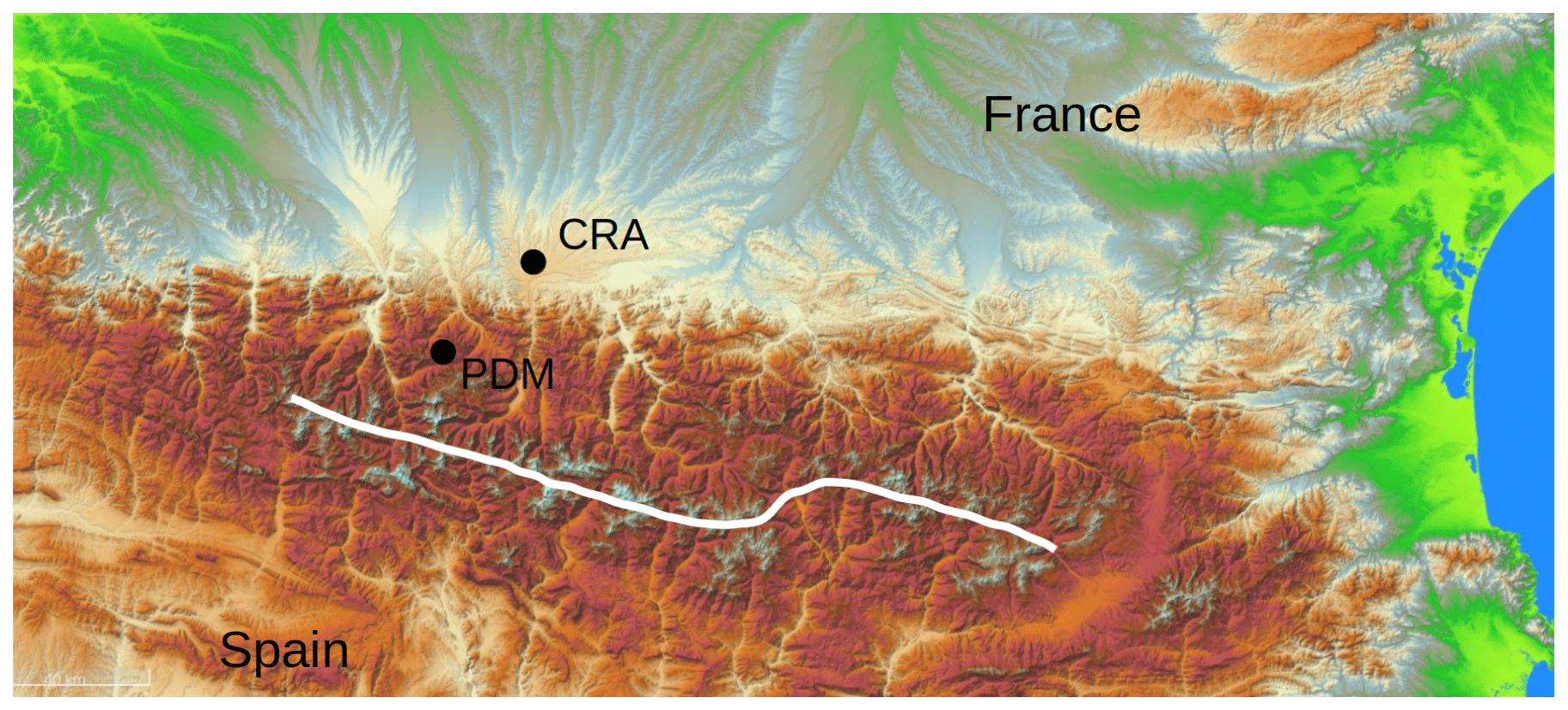
Figure 1 Locations of the measurement sites. The white line represents the main Pyrenean watershed.

Historical measurement series at the PDM for temperature (Bücher and Dessens, 1991, 1995), relative humidity and cloud cover (Bücher and Dessens, 1995), rainfall (Bücher and Dessens, 1997), and ozone (Marenco et al., 1994) have been studied. The latter authors showed that ozone trends measured at the PDM throughout the twentieth century were in line with data from other European high-altitude sites. This suggested that high-altitude sites have the capacity to provide atmospheric composition measurements representative of a vast geographic area, at least when long time periods are considered. In the same vein, Chevalier et al. (2007) found close agreement between multi-year averaged ozone data from high-altitude stations in Europe, including the PDM, and from airborne measurements in the free troposphere at the same altitude. Henne et al. (2010) compared many European air quality observatories by means of a particle dispersion model and found that the PDM and a few other sites are, for the most part, remote from anthropogenic emissions. Mountain sites thus appear to be suitable sites to provide baseline concentrations that are representative of the free troposphere, remote from local sources (Parrish et al., 2014), and in turn representative of the global scale (Keeling et al., 1976).

Nevertheless, mountain observatories, even those found on the peaks, lie in the mountain boundary layer and are not representative of the regional free troposphere 100 % of the time. In the mountains, enhanced turbulence and specific airflows are created, and this may drag surface air masses to the mountaintops and then affect the gas and aerosol concentrations (Serafin et al., 2018; Henne et al., 2004; Griffiths et al., 2014). Using three main processes combining the vertical transport of boundary-layer air and mixing with background air during the recent history of the air mass, Griffiths et al. (2014) point out the potential influence of local to regional sources on air composition measurement at the Alpine station Jungfraujoch (3600 m a.s.l.), although this is also transposable to at least the PDM and likely also to other high-mountain stations around the world. These processes are (i) thermally driven mountain boundary layers and anabatic flows; (ii) terrain-forced flows such as foehns, in which synoptic winds significantly interact with the topography; and (iii) deep vertical mixing over the surrounding plains followed by horizontal advection to the mountains.

These three types of processes are relevant to the P2OA. Thermally induced circulations are generated by differential heating of the slope vs. valley atmospheres or the mountain vs. plain atmospheres. This results in anabatic (upward) flows during the day and, conversely, katabatic (downward) flows at night at a variety of spatial scales: slope flows, valley flows, and plain–mountain flows (Whiteman, 2000). There has been a particular focus on thermally driven circulations and their impact on the atmospheric composition for many mountain sites (e.g. Lugauer and Winkler, 2005; Necki et al., 2003; Forrer et al., 2000, among many others). At the P2OA specifically, such studies have been conducted by Gheusi et al. (2011), Jiménez and Cuxart (2014), Tsamalis et al. (2014), Román-Cascón et al. (2019), and Hulin et al. (2019). All these studies reveal a significant diurnal impact of thermally driven circulations on atmospheric composition and, more specifically, at the PDM, a daytime enhancement of any atmospheric species that are generally more concentrated in the boundary layer than in the free troposphere (e.g. water vapour, radon, CO, CH₄, etc.), and conversely a daytime depletion in species that are less concentrated in the (rural) boundary layer than in the free troposphere (typically ozone and CO₂ during the vegetation growing season). This suggests that the regional boundary layer is a partial or the only influence at the PDM in the daytime. Studying a case of anabatic transport from the CRA to the PDM with a simple numerical transport model constrained by ozone measurements, Tsamalis et al. (2014) found a possible range of 14 % to 57 % for the percentage of boundary-layer air mixed into free-tropospheric air in the daytime. Hulin et al. (2019) tested three methods for detecting thermally induced circulations in the P2OA area, which will be used later in the present study (Sects. 2.3.2 and 4.3).

The second phenomenon which occurs frequently at the P2OA is the foehn, a hydraulic-like flow pattern that occurs on the lee side of a mountain barrier when the synoptic flow is forced to flow over and plunge beyond the crest line (Whiteman, 2000). In the P2OA configuration (on the northern side of the Pyrenees, Fig. 1), the foehn is a warm, dry, strong, downslope, southerly wind affecting the northern flank of the Pyrenees. In the case of deep foehns, the downslope flow may even reach the surface at CRA in the foothills. South foehn cases in the Pyrenees were studied during PYREX, which was a field campaign in the Pyrenees relating to clear-air turbulence (Bougeault et al., 1997). However, to our knowledge, no south foehn climatology is available for the Pyrenees. The impact of the foehn on ozone has been studied at an Italian Alpine foothill station that is subject to north foehn winds (Weber and Prévôt, 2002), with results showing strongly reduced O₃ levels during foehn events in summer and slightly increased levels in summer. Forrer et al. (2000) confirm the occurrence of those ozone variations at the Jungfraujoch and show strongly increased CO and NO_x concentrations.

The third phenomenon is vertical mixing in the plain due to deep convective systems followed by advection towards the PDM. This transport occurs at a regional scale. Forrer et al. (2000) and Zellweger et al. (2003) thoroughly studied its impact on CO and NO_x concentrations and showed that it has a similar impact on concentrations to the other two phenomena.

Another common way to analyse air composition data at mountain sites is to track (usually at a larger continental scale) the air mass origin using backward trajectories or dispersion models. The composition measurements are then sorted by geographical source region (e.g. Cristofanelli et al., 2013 for Campo Imperatore, central Italy, as the receptor site; Perry et al., 1999 for Mauna Loa, Hawaii; Tso et al., 2022 in the UK; Gaudel et al., 2015 for the Observatoire de Haute Provence, France; Cui et al., 2011 and Loeoev et al., 2008 for the Jungfraujoch; among many). The latter two studies in the list highlight differences in ozone concentration and other chemical species such as CH₄ and CO that depend on whether the air masses are influenced by the local planetary boundary layer or long-range advection. In Cristofanelli et al. (2013), differences in ozone concentrations at Campo Imperatore (in the Abruzzi massif) are shown; these depend on whether the air masses have a maritime (Mediterranean) or continental (European) origin. At this site, continental air masses tend to bring air masses with higher ozone contents.

A survey of local or regional weather regimes also brings useful information, since the meteorology may affect the atmospheric composition at mountain sites in many, and often complex, ways due to the occurrence of different transport and mixing patterns at all scales, contrasting conditions for photochemistry or atmospheric scavenging by precipitation, etc. Thus, sorting composition data by weather type may be a fruitful approach. A rich variety of methods to build meteorological classifications are encountered in the literature. Weather regimes may be computed from pressure fields using global weather models, and the resulting classification is generally intended for large geographical areas, e.g. Europe (Cortesi et al., 2019; Neal et al., 2016) or the Mediterranean Basin (Giuntoli et al., 2021). At smaller scales, studies aiming at characterizing weather regimes at specific measurement sites exist for urban areas (e.g. Hidalgo and Jougla, 2018 for Toulouse, France; Hodgson and Phillips, 2021 for Birmingham, United Kingdom). In the latter study, the authors use local meteorological data and an algorithm for hierarchical clustering to build a meteorological classification.

Tso et al. (2020) used local observations in the UK and k-means clustering to define a limited number of local meteorological “states” (i.e. regimes). Among the variables in the environmental database they mined, they distinguished “state variables”, which were used for the clustering, from “observational variables” (e.g. moth and butterfly counts), for which the statistics for different states were considered separately. Then, they used extreme quantiles in the different states as criteria to flag outliers in the observational variables.

For the Alps, a classification of weather types has existed for a long time – since 1945. It was devised by Schüepp (1979) and is described in Stefanicki et al. (1998). This synoptic weather type classification system (SYNALP) involves determining five parameters (speed of the surface geostrophic wind, direction and speed of the 500 hPa wind, height of the 500 hPa surface, and baroclinicity), which are measured or computed for a circular area (diameter: 444 km) covering Switzerland. Stefanicki et al. (1998) studied the frequency of changes in those weather types since 1945 and showed an increase in convective days in winter at the expense of advective days. In addition, in Collaud Coen et al. (2011), SYNALP was utilized to analyse a long time series of chemical species (including aerosols and CO) measured at the Jungfraujoch to assess the influence of free tropospheric air and air advected from the boundary layer to the Jungfraujoch. However, no such meteorological classification exists for the Pyrenean area.

Our main objective in this study is to provide a classification of observation days at the P2OA sorted by typical synoptic weather regimes and to establish statistics for all variables – especially gas and particle concentrations – in the different regimes. The clustering will allow us to track the occurrences and the characteristics of the weather regimes and to relate them to the chemical concentrations measured at the PDM. Our methodology is thus very similar to the approach of Tso et al. (2020), since we will use a set of 23 meteorological variables as state variables and then compare the statistical distributions of the concentrations of six atmospheric species (our observational variables) in the different weather regimes (states). Our final goal, however, is different: while Tso et al. (2020) are ultimately concerned with data quality control and outlier flagging, our main intent here is to characterize the main influences of the meteorology on the atmospheric composition at our observatory.

We chose to use only data produced locally on the platform, and to use hierarchical clustering as the classification method. This approach has the advantage of being easily applicable to other observatories by local investigators who have easy access to data measured in situ. Also, large-scale model fields may miss local meteorological specificities (due to a small-scale topography, field heterogeneity, etc.) that are otherwise captured by in situ measurements.

Hierarchical clustering allows us to obtain weather patterns without any preconceptions about the local weather. It is a classification method that groups data vectors (in the multi-dimensional space of all considered variables) depending on their closeness (more details are given in Sect. 2.2). Carried out on a data set of meteorological variables, it will generate clusters with similar meteorological characteristics. Such clusters can be linked to weather regimes, and hierarchical clustering has thus been widely utilized for this goal (e.g. Kalkstein et al., 1987; Ng et al., 2020; Hodgson and Phillips, 2021, among many other references).

Details of the measurements and the database, the data processing, the clustering method, and the diagnostic tools are provided in Sect. 2. Meteorological regimes obtained from the clustering are presented in Sect. 3 and are then compared using diagnostic tools that are designed to focus on specific meteorological phenomena (Sect. 4). Finally, we consider and compare the statistics of the atmospheric composition variables available at the PDM for the different meteorological clusters (Sect. 5). Finally, conclusions are drawn, and perspectives are suggested, in Sect. 6.

2 Methods

2.1 Data set

2.1.1 Database and hourly data set

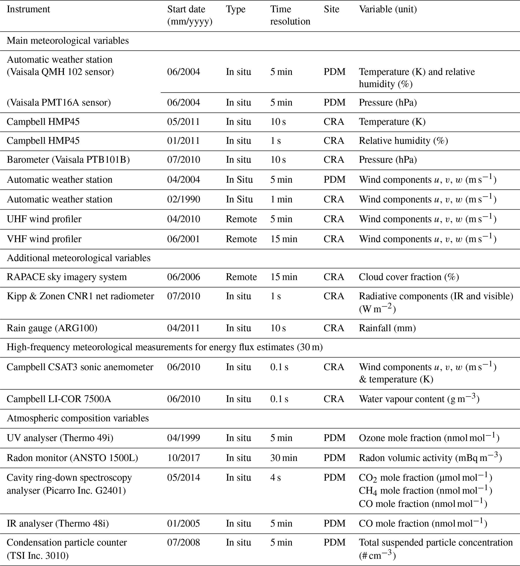
The time frame of the present study runs from 1 January 2015 to 31 December 2019. This period was chosen to optimize the data coverage for a panel of atmospheric measurements at both P2OA sites. All the instruments used in our study, along with technical details and the output variables, are listed in Table 1.

Table 1 Instrumentation characteristics.

We adopted coordinated universal time (UTC) for the whole study because this time standard is almost the same as local solar time at the PDM, given that the PDM is located at longitude 0.14^∘ E.

As the data were collected at different time resolutions (Table 1), the first data set was built on a synchronized hourly basis. Thus, the values provided for a given timestamp (e.g. 27 May 2018, 08:00:00 UTC) represent averages of any data available in the 1 h interval beginning at this timestamp (08:00:00–08:59:59). Even though the hierarchical clustering detailed below (in Sect. 2.2) is based on a final daily data set, the construction of an intermediate hourly data set was needed for some of the diagnostic tools (Sect. 2.3) that work on an hourly basis – for example, the detection of diurnal cycles.

We used an extensive set of meteorological data recorded routinely at the PDM (2877 m a.s.l.) and the CRA (600 m a.s.l.) stations (data available online at https://p2oa.aeris-data.fr), which included temperature, relative humidity, and pressure measured by standard weather stations, cloud occurrence above the CRA, and wind measured at different levels above the ground up to the mid-troposphere, as detailed here. At the CRA, a 60 m tower provides meteorological measurements at both low and high frequencies. We considered the measurements of mean wind from a sonic anemometer installed on this tower (10 m) and from two wind profilers. Both provided the three components of the wind, but over different vertical ranges and resolutions. The UHF (1274 MHz) wind profiler scans the lower troposphere from 100 m up to 6 km above the ground with a vertical resolution of 75 m. The VHF (45 MHz) wind profiler covers the range 1.5–16 km a.g.l. from the mid-troposphere to the lower stratosphere with a 375 m resolution. Technical details are available in Campistron et al. (1999) for the VHF and in Jacoby-Koaly et al. (2002) for the UHF. At the PDM, we considered standard measurements of wind at 2 m above the ground obtained with a sonic anemometer (note that the surface wind at the PDM is affected by buildings in some wind sectors; Hulin et al., 2019).

The ground-based anemometers and the two wind profilers at the CRA provided wind time series for many vertical levels. However, the wind data at two close levels (e.g. 100 m and 200 m above the ground) are strongly correlated and provide redundant information. Thus, we selected a sufficient number of key vertical levels to capture the vertical structure of the dynamics from the ground up to the mid-troposphere, but not too many levels in order to avoid redundancy. Therefore, we chose the surface levels at the PDM (2877 m a.s.l.) and at the CRA (600 m a.s.l. + 10 m a.g.l. = 610 m a.s.l.) and higher levels at 750, 1600, and 2850 m a.s.l. above the CRA.

Additional observation data were also considered and are listed in Table 1. In order to consider cloud cover, a full-sky imager was used to retrieve the cloud-cover fraction by means of the algorithm ELIFAN (Lothon et al., 2019) based on the red-over-blue ratio and a blue sky library. We used the rain gauge at CRA for precipitation estimations. Finally, the surface energy and sensible and latent heat fluxes were added to take account of surface/atmosphere interactions. Heat fluxes were calculated based on 30 min samples from high-rate measurements (10 Hz) of temperature, wind, and moisture with the EddyPro^® software (version 6.2.0).

To study the impact on the atmospheric composition measured at the PDM, we considered measurements of the atmospheric composition (CH₄, CO₂, CO, O₃) and aerosol particle numbers (Hulin et al., 2019, and references therein for details of the instruments). Note that the CO data series used here is a composite of data from two instruments: an IR absorption analyser and a cavity ring-down spectrometer (Table 1). Both instruments were needed in order to upgrade the data coverage over the studied period to a satisfactory level. Radon volumic activity was also included in the present data set, even though the radon monitor has only been in operation since October 2017.

2.1.2 Daily data set suitable for separating synoptic weather regimes

Day-to-day changes are relevant to our aim of characterizing the specific impact of the synoptic meteorological context, as they drive the clustering of meteorological data, but the seasonal trends (e.g. in temperature) and the variations related to the diurnal thermal cycle are not. The multi-annual trends presented by some variables (e.g. CO₂) are not in our scope either. Therefore, from the basic hourly data set detailed in the former paragraph, we built a final daily data set composed of 1826 d for which (i) the diurnal variations were neutralized by averaging on a daily basis and (ii) multi-annual and seasonal trends were characterized by means of a nonlinear least-squares regression and then removed.

The regression function contains a linear part in order to model the long-term variation and a 1-year periodic part with sinusoidal components (up to the fourth harmonic) to model the seasonal trend. Thus, the generic regression function for any variable X is written

$$\begin{array}{}\text{(1)}& \begin{array}{rl}X\left(t\right)& =a_{\mathrm{1}}+a_{\mathrm{2}}t+a_{\mathrm{3}}\sin \left(\mathrm{2}\mathit{\pi }t\right)+a_{\mathrm{4}}\cos \left(\mathrm{2}\mathit{\pi }t\right)\\ & +a_{\mathrm{5}}\sin \left(\mathrm{4}\mathit{\pi }t\right)+a_{\mathrm{6}}\cos \left(\mathrm{4}\mathit{\pi }t\right)+a_{\mathrm{7}}\sin \left(\mathrm{6}\mathit{\pi }t\right)\\ & +a_{\mathrm{8}}\cos \left(\mathrm{6}\mathit{\pi }t\right)+a_{\mathrm{9}}\sin \left(\mathrm{8}\mathit{\pi }t\right)+a_{\mathrm{10}}\cos \left(\mathrm{8}\mathit{\pi }t\right)\end{array}\end{array}$$

(with t being expressed in years).

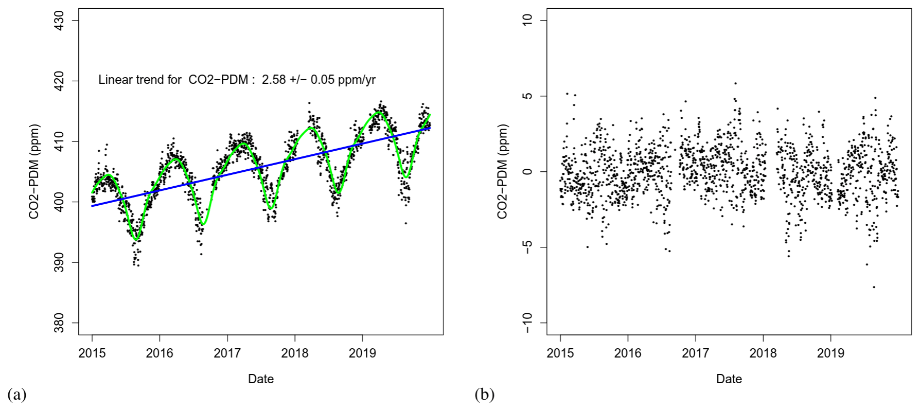
Figure 2 Time series of CO₂ measurements at the PDM for our time frame. In panel (a), the blue line represents the long-term trend in CO₂ and the green line represents the seasonal trend. Both trends are computed by nonlinear least-squares regression. Panel (b) shows the obtained CO₂ anomaly time series.

After subtracting the long-term and seasonal trends from the daily averages, we obtained what we call “anomalies” in the rest of the article. For example, in Fig. 2a, we can see the original time series of CO₂ daily averages as well as the modelled long-term and seasonal trends. Figure 2b displays the resulting CO₂ anomaly time series. For the four irradiance variables, this treatment failed to neutralize the seasonal variability. As an alternative process to compute the daily anomalies, we divided the daily averages by a moving average computed over 2 weeks.

Table 2 List of variables in the daily data set.

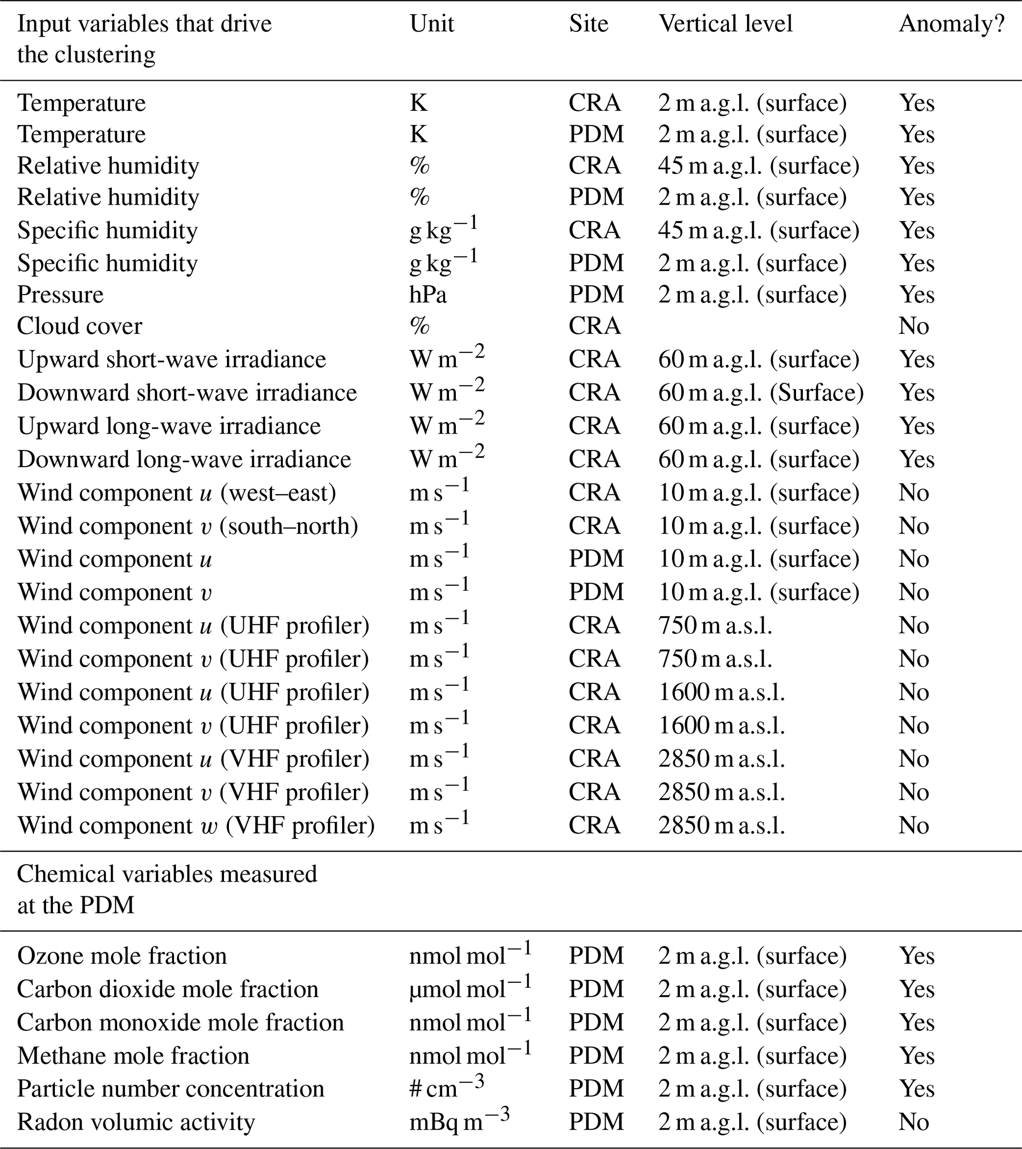
These processes were applied for all variables tagged “Yes” in the “Anomaly” column in Table 2, with the other variables being simple daily averages. The 23 variables which drive the clustering are listed in the upper part of Table 2. All other variables were used to conduct statistical analyses within the obtained clusters but did not influence the clustering.

2.2 Hierarchical clustering

Hierarchical clustering is a non-supervised classification method which builds groups of points that are closest to each other in the multi-dimensional space of all considered variables. In our case, a point – or event – in this space represents a vector formed by all variables of the daily data set associated with a given date. Thus, the events that fall into each cluster tend to share common characteristics.

The key requirement in hierarchical clustering is the ability to assess distances in this space. Hierarchical clustering is an iterative method where, at each step, the closest points or groups of points (clusters) are progressively merged into a new cluster (Wilks, 2011).

Over and above the way distances between two points are computed (the Euclidean distance is usually used and was adopted in the present study), hierarchical clustering methods differ in the way distances between clusters are assessed. There are three main methods: Ward's method (based on the sum of the squared errors between the two clusters), centroid (the distance between the centroids of the clusters), and linkage (complete, single, or average). In complete and single linkage, the maximum and minimum distances between points from the two groups are retained, respectively, whereas average linkage evaluates the average cluster-to-cluster distance (Wilks, 2011). Ward's method is often used in meteorological studies due to its ability to form groups with balanced populations (Kalkstein et al., 1987). These methods were applied to a meteorological data set and compared in Kalkstein et al. (1987). In their study, average linkage (with Euclidean distance) turned out to be the most suitable method, as it minimized the variance within clusters compared to Ward's method and the centroid method.

For this reason, we chose the linkage method for our study, as we needed the minimum variance within the cluster (well-defined weather regimes). With our data set, however, single and average linkage resulted in one very large group and many single-day groups. Only the complete linkage method provided groups with more balanced populations, and hence this method was chosen for this study.

Some past studies that used hierarchical clustering of meteorological data adopted a different approach than ours. A principal component analysis (PCA) was first performed on the input meteorological data. Then hierarchical clustering was applied to the principal components. This process was performed to counteract the interdependence of the input variables. This interdependence exists when studies focus on a zone with different measurement sites but few variables (e.g. Degaetano, 1996; Bravo et al., 2012; Pineda-Martínez and Carbajal, 2017). PCA is also needed in studies that include rainfall in the clustering due to its shape (e.g. Hodgson and Phillips, 2021; Ramos, 2001; Ng et al., 2020). Nevertheless, we did not use PCA in our study. To avoid redundancy issues, we carefully chose the input variables as described in the previous section. In addition, before the clustering, we centred and scaled the data set.

2.3 Diagnostic tools

What we call diagnostic tools in this study are additional indicators computed mostly from data from our hourly or daily data sets, but also, in some cases, from additional (rain gauge) observations or an extra data source (NCEP (National Centers for Environmental Prediction) reanalysis data). Our main motivation is to further characterize the groups emerging from the hierarchical clustering, with a focus on specific atmospheric properties (e.g. vertical structure) or phenomena (e.g. foehn).

Philibert et al. (2023)

Table 3 Diagnostic tools used in the study. (See text for details.)

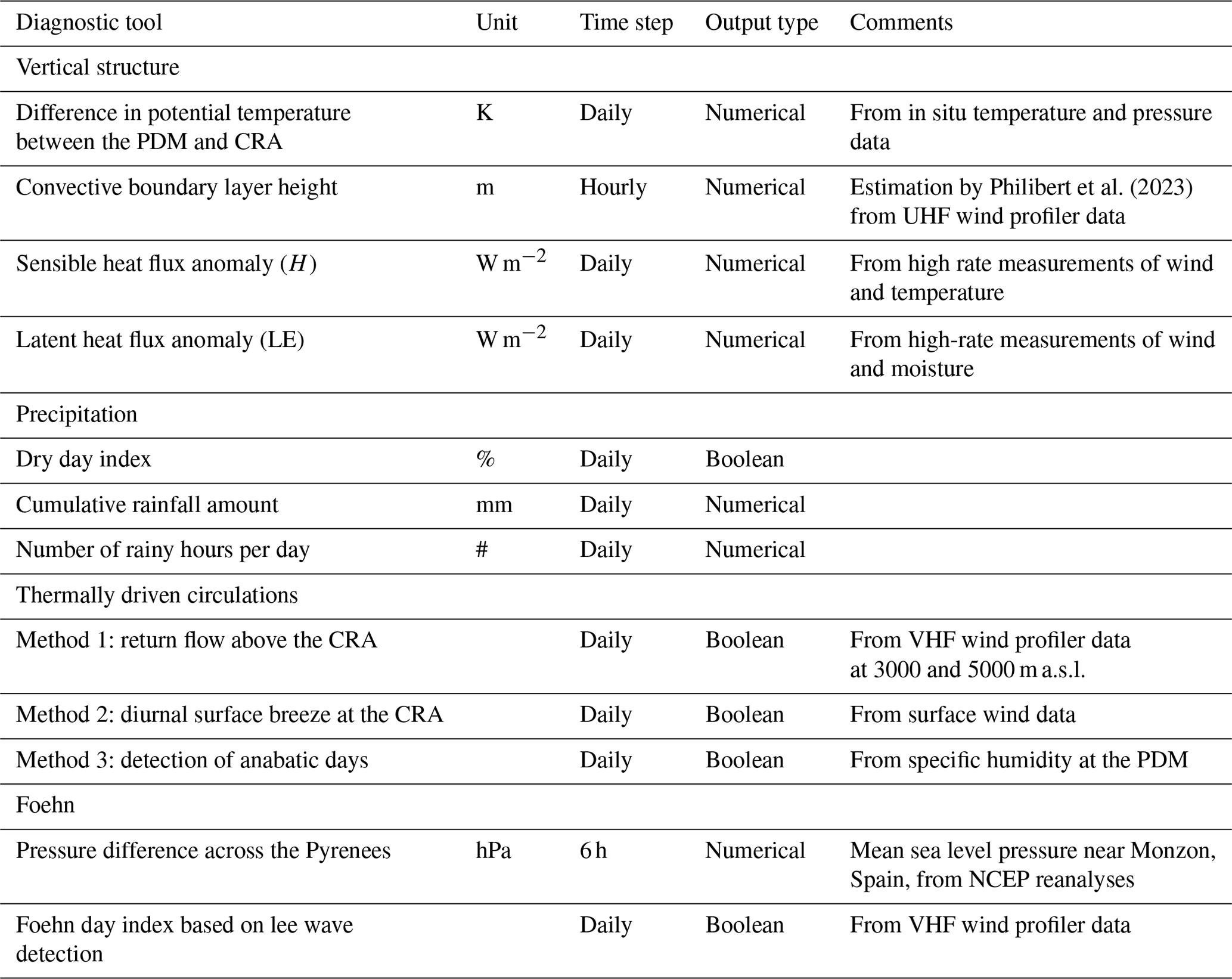
All the diagnostic tools are summarized in Table 3. They were computed on either an hourly or daily basis (depending on the need) and separated into three thematic groups: atmospheric vertical structure and precipitation, thermally driven circulations, and foehn.

2.3.1 Atmospheric vertical structure and precipitation

The first two diagnostic tools described here concern the vertical structure of the lower troposphere. Potential temperatures at both the CRA and PDM sites were computed from surface temperatures and pressures, so the mean daily difference ($\mathrm{\Delta }\mathit{\theta }={\mathit{\theta }}_{\mathrm{PDM}}-{\mathit{\theta }}_{\mathrm{CRA}}$) between stations gives us an approximate but simple indication of the stability of the lower atmosphere in the area.

Another key variable is the daytime convective boundary layer (CBL) depth (Z_i), which is the depth over which any scalar may be mixed by convection in a short time range, generally less than 1 h (Stull, 1988). This variable can be estimated hourly at the CRA with the UHF wind profiler. Here we use estimations from Philibert et al. (2023), based on the fact that the turbulent CBL is topped by a temperature and moisture inversion and a drop in turbulence. Z_i estimations are thus deduced from the local maximum reflectivity in the low troposphere inversely weighted by the intensity of turbulence as well as by criteria relating to temporal and spatial continuity. Sensible and latent heat fluxes near the ground were also considered as diagnostic tools in order to take into account surface/atmosphere interactions and relate them to the observed CBL depth. We computed the anomalies in those fluxes in the same way as for other variables (such as temperature), as described earlier.

Completing the moisture and cloud cover measurements, rainfall data are relevant but complex to handle in statistical analyses because their distribution is very heterogeneous: it has a value of zero a large fraction of the time and includes scarce rainfall episodes with large ranges of intensities and durations. We thus computed three values: (i) for each cluster of days, we computed the total number of dry days (defined as days with zero rainfall); for each day, we computed (ii) the number of rainy hours (those with non-null hourly rain amounts) and (iii) the total amount of rain. The two diagnostics of “cumulative rainfall amount” and “number of rainy hours per day” were used to characterize the rainy days of each cluster. Thus, they were computed based only on the rainy days of each cluster. This prevented the dry days from introducing a bias into the statistics when assessing the rain intensity or type during rain events.

2.3.2 Thermally driven circulations

Thermally induced circulations in mountainous regions are local air motions induced by the heating of the air along mountain slopes. Close to the surface, air moves upward (anabatic transport) in the daytime and downward (katabatic transport) at night. Such transport may occur at various spatial (and temporal) scales: at the scale of each single radiated slope, at the scale of secondary and primary valleys, and at the scale of the mountain massif itself (Whiteman, 2000).

Under a clear sky and weak synoptic wind conditions, plain-to-mountain transport develops in the daytime up to the regional scale (e.g. up to 100 km in the Bavarian Alpine foothills, Lugauer and Winkler, 2005). A closed circulation cell may form, with a return flow at altitude, oriented from the mountain to the plain. Such circulation and its impact on the atmospheric composition were specifically studied at the P2OA by Hulin et al. (2019). Those authors proposed three detection methods that will be applied to our data here. Technical details about the methods are available in their article. The main concepts are summarized here.

Method 1 aims at detecting the presence during the daytime of a return flow above the CRA by comparing the wind at 3000 m (which could be affected by the return flow) and that at 5000 m (presumed to be unaffected). The main idea is to find a significant enhancement of the southern component of the wind at 3000 m that would be negligible at 5000 m in the interval 10:00–16:00 UTC (but not before or after).

Method 2 aims at detecting anabatic/katabatic surface breezes at the CRA by considering the diurnal alternation in wind direction from a wide north-east sector (330–110^∘) during daytime (11:00–14:00 UTC) to the south-east (130–190^∘) at night (21:00-02:00 UTC).

The above two methods result in daily boolean flags which show whether or not a thermally driven circulation is detected for the current day.

Finally, Method 3 consists of ranking the days of the data set depending on the influence of anabatic transport on the water vapour content measured in situ at the PDM. This influence can be quantified using the amplitude of the diurnal cycle of specific humidity as a proxy. The larger the amplitude, the more efficient the anabatic transport of humid air from the valleys to the PDM. This method was originally designed by Griffiths et al. (2014) for radon measurements. However, radon data were not available for the period (2006–2015) covered by the study by Hulin et al. (2019), so they alternatively used specific humidity, as suggested by Griffiths et al. (2014). In our case, specific humidity and radon data are simultaneously available from late 2017 to the end of 2019, a period for which we checked that rankings based on both variables provided consistent results (not shown). In the following, we therefore only consider the ranking based on specific humidity, as humidity data were available at the PDM for the whole time frame of the study. Method 3 assigns a rank to each day according to the degree of anabatic influence: the day ranked 1 has the diurnal cycle with the greatest weight in the composite mean diurnal cycle computed over all days; then the amplitude decreases as the rank increases until it vanishes at a threshold rank (the day ranked 850th), after which a diurnal cycle cannot be observed. So, the method allows us to distinguish anabatic days (ranked before the threshold) from non-anabatic days (ranked after). All details can again be found in Hulin et al. (2019).

2.3.3 Foehn

Jansing et al. (2022) define the generic term foehn as “downslope winds […] in the lee of mountains […] associated with a distinct warming and a decrease in relative humidity of the air on the lee side of the orographic barrier”. On the northern side of a mountain barrier, which is the case at the P2OA, foehn situations (south foehns) require south-westerly to southerly synoptic flows.

Foehn occurrence and characteristics will be studied by means of two diagnostic tools. The first is the horizontal pressure difference across the Pyrenees. A foehn, which is in essence a cross-barrier wind, is typically associated with a pressure dipole across the mountain chain (Bessemoulin et al., 1993). In the case of a south foehn, there is therefore a positive pressure difference between the south and the north of the chain. This pressure drag increases with the intensity of the foehn (Lothon et al., 2003; Drobinski et al., 2007). To compute this diagnostic tool, pressure data were needed from the southern side of the Pyrenees (Spain). We used mean sea level pressure data at 6 h intervals from NCEP global reanalysis data (https://rda.ucar.edu/datasets/ds083-2/, last access: 12 December 2023) taken at the nearest grid point from Monzon (130 km south of the CRA, province of Huesca, 41^∘54^′00^′′ N, 0^∘11^′00^′′ E). For pressure on the French side, we had two possibilities: the actual pressure measured at the CRA (reduced to mean sea level) or the pressure data from NCEP reanalysis at the closest grid point. Greater differences from Monzon were found with the measured pressure (suggesting that NCEP reanalysis can underestimate the foehn intensity due to the smoother terrain in the model), so we retained the measured pressure at the CRA for the calculation.

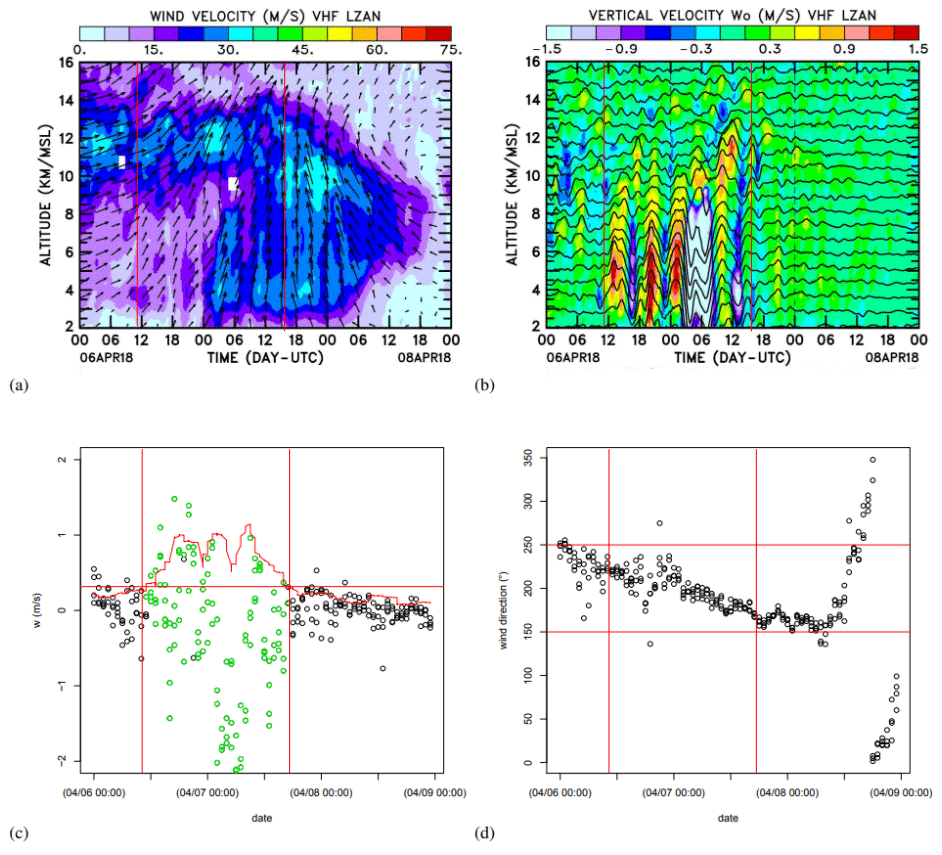
Figure 3 Time–height plots of the horizontal (a) and vertical (b) wind measured by the VHF wind profiler on 6–8 April 2018, presented as an illustration of a foehn event. In (a), an arrow towards the top indicates a southerly flow and an arrow towards the right indicates westerly flow. Times series of the vertical wind component w (c) and wind direction (d) at 2850 m a.s.l. for the same days are shown. In all four panels, vertical red lines represent the beginning and end of the detected foehn episode. In panel (c), the red curve represents the rooted variance (i.e. standard deviation) of w over a 6 h running interval, while the horizontal red line represents the threshold for lee wave detection ($\sqrt{\mathrm{0.1}{\mathrm{m}}^{\mathrm{2}}{\mathrm{s}}^{-\mathrm{2}}}\approx \mathrm{0.32}$ m s⁻¹). Green circles identify the data points for which the variance criterion is met. In panel (d), the two horizontal red lines represent the two wind direction thresholds used in the detection method.

The second diagnostic tool is based on the occurrence of mountain lee waves, as seen over the CRA with the VHF wind profiler. During a foehn event, the south to south-westerly flow generates mountain waves in the lee of the Pyrenees chain, which can be observed throughout the whole troposphere. Figure 3 shows an example of such a situation, as seen by the VHF wind profiler. This figure shows how the strong southerly flow (Fig. 3a) can be associated with large variations in vertical air velocity (Fig. 3b), a signature of mountain lee waves. The intensity of vertical tropospheric oscillations is quantified here as the variance of the vertical wind w at 2850 m a.s.l. computed over a running 6 h interval from the original 15 min VHF-profiler data. A data point is flagged as a lee wave occurrence if the horizontal wind direction is between 150 and 250^∘ and if the w variance exceeds 0.1 m² s⁻². Corresponding time series of vertical velocity, variance, and wind directions are displayed in Fig. 3c and d along with the identification of the lee wave occurrence with this method. We considered a foehn hour to be any hour with at least 50 % of the 15 min data points flagged as a lee wave. Finally, in order to extract a daily diagnostic value, we consider a foehn day to be any day containing at least 6 h of foehn.

3 Meteorological regimes from the hierarchical clustering

3.1 Clustering implementation and cut of the clustering tree

A hierarchical clustering algorithm was applied (with the options detailed in Sect. 2.2) to a collection of 1826 events (observation days from 1 January 2015 to 31 December 2019), each composed of the 23 variables listed in Table 2 (upper part). Gas and particle concentrations (Table 2, lower part) were not included in the variables driving the clustering, with the aim being to obtain regimes based purely on the local meteorology. Nevertheless, statistics for gas and particle variables were considered for each meteorological cluster, and they will be presented in Sect. 5.

Our choice to cut the clustering process at the step with six clusters allowed us to have a minimum number of clusters while keeping the size of the largest cluster below 50 % of the total number of observation days (1826). We thus obtained three major (i.e. highly populated) clusters (containing 622, 720, and 418 d: hereafter Clusters 1, 2, and 3, respectively) and three minor clusters (containing 20, 33, and 13 d: hereafter Clusters 4, 5 and 6, respectively).

3.2 Analysis of the three major clusters

3.2.1 Thermodynamic variables

To explore the characteristics of the major clusters, we first summarized the statistical distributions of the main thermodynamic variables within each cluster by means of box-and-whisker plots (hereafter “boxplots”) in Fig. 4. This shows that whatever the variable or class, the distributions are centred on median values that show marked differences between clusters (even though the interquartile ranges overlap in most cases).

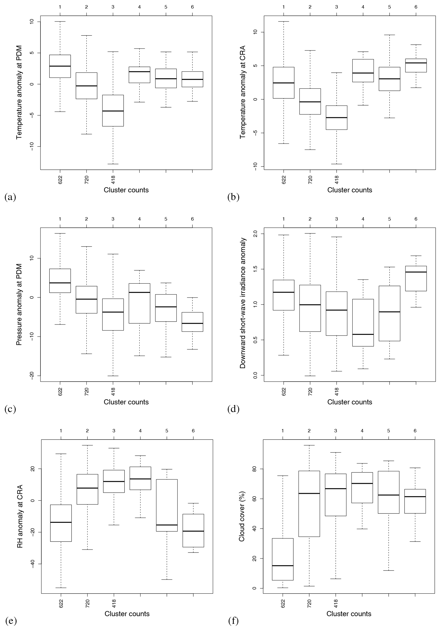
Figure 4 Boxplots of the temperature anomaly (K) at the PDM (a) and the CRA (b), the pressure anomaly at the PDM (hPa) (c), the downward short-wave irradiance anomaly (W m⁻²) at the CRA (d), the relative humidity anomaly (%) at the CRA (e), and the cloud cover (%) above the CRA (f).

Considering the temperature anomaly at the PDM, which represents the deviation from the expected seasonal value, Clusters 1 to 3 have median values of +2.5, −0.5, and −4.5 K, respectively (Fig. 4a). A similar hierarchy also appears in the temperature anomaly at the CRA (+2.5, −0.5 and −3.0 K, respectively; Fig. 4b), the pressure anomaly at both stations (Fig. 4c for the PDM; that for the CRA is not shown but is similar), and the solar (downward short-wave) irradiance (Fig. 4d). We also noticed a reversed pattern (i.e. increasing median values from Cluster 1 to Cluster 3) for relative humidity (Fig. 4e for the CRA; that for the PDM is not shown) and cloud cover at the CRA (median values of 15 %, 65 %, and 70 %, respectively; Fig. 4f).

In brief, Cluster 1 contains warmer, drier clear-sky and high-pressure days, suggesting anticyclonic fair-weather conditions; Cluster 3 contains colder, more humid, cloudier low-pressure days, suggesting disturbed weather; and Cluster 2 contains days with intermediate characteristics.

3.2.2 Wind

Hodographs of the synoptic wind from the VHF profiler (at 2850 m a.s.l., corresponding to the altitude of PDM; Fig. 5) show that in Cluster 3, the wind blows mostly from the north-west quadrant. In addition, the wind strength is above 10 m s⁻¹ a large part of the time and exceeds 20 m s⁻¹ on some days, whereas there are much fewer strong wind days in Cluster 2, and almost none in Cluster 1.

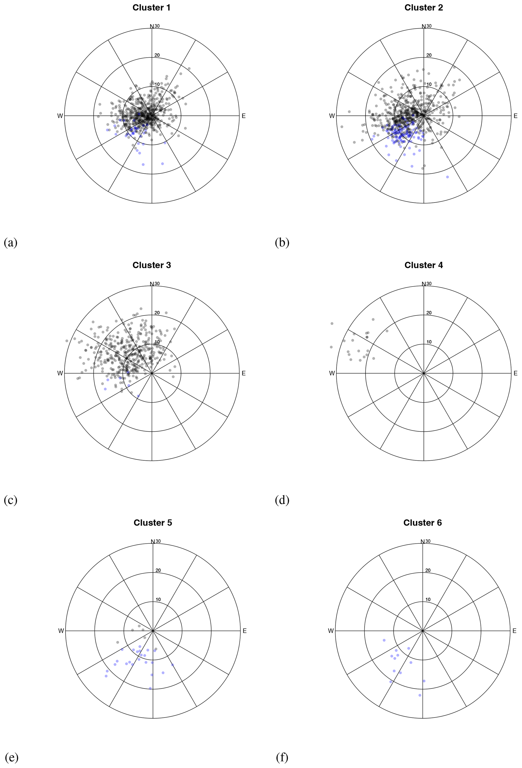
Figure 5 Hodographs of the daily mean wind vectors measured by the VHF profiler at 2850 m a.s.l. for the six clusters (a–f). Wind speed (radius) is in m s⁻¹. Blue points correspond to days flagged as foehn days based on lee wave detection (details in Sect. 2.3.3).

In western Europe, strong north-westerly winds are typical of disturbed weather (with low temperature and high cloud cover and rainfall, e.g. Giuntoli et al., 2021). In Clusters 1 and 2, the wind may blow from a larger variety of sectors – there are a few days with southerly or north-easterly wind but the majority of the days have south-westerly to north-westerly wind. However, Cluster 2 also shows strong (10–20 m s⁻¹) north-westerlies that are almost absent in Cluster 1. Thus, Cluster 2 contains several days with similar wind conditions to Cluster 3. Cluster 2 also shows frequent days with strong southerly to south-westerly wind, potentially corresponding to foehn conditions.

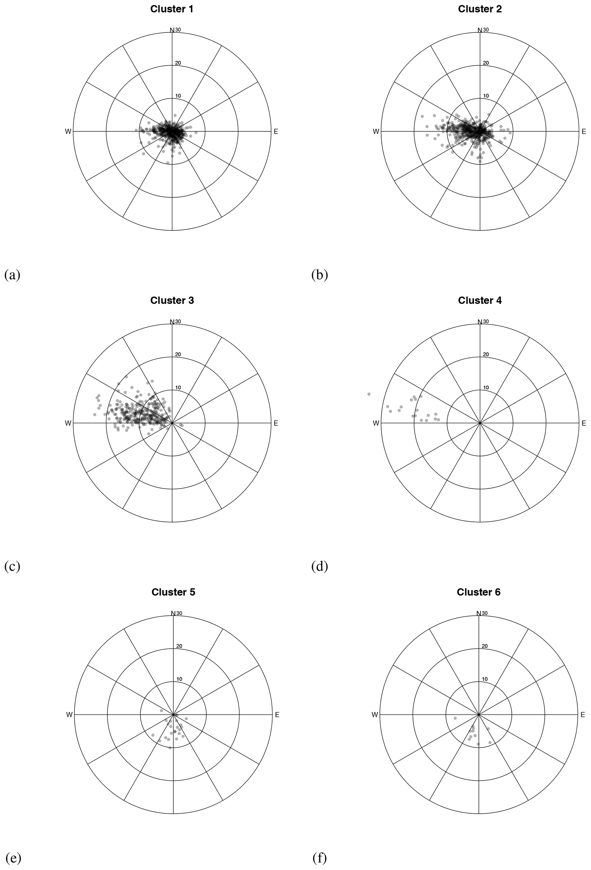
Figure 6 Hodographs of the daily mean wind vectors measured by the UHF profiler at 1600 m a.s.l. for the six clusters (a–f). Wind speed (radius) is in m s⁻¹.

Studying the wind above the CRA but at a level below the Pyrenean crest (1600 m a.s.l., Fig. 6) provides further information. In Cluster 3, the wind is concentrated in a narrower sector (between 270 and 300^∘) than higher in the mid-troposphere. A plausible explanation is that the synoptic north-westerly flow is locally channelled along the Pyrenees at 1600 m. This channelling effect can also be seen in Clusters 1 and 2 from the west, but also from the east in some cases. When the synoptic wind is from the south-west, air masses may not have sufficient kinetic energy to flow over the Pyrenees, and in this case, they flow around the barrier, with possible channelling on the lee side. Clusters 1 and 2 also contains a few days with sustained southerly wind, presumably corresponding to south foehn events.

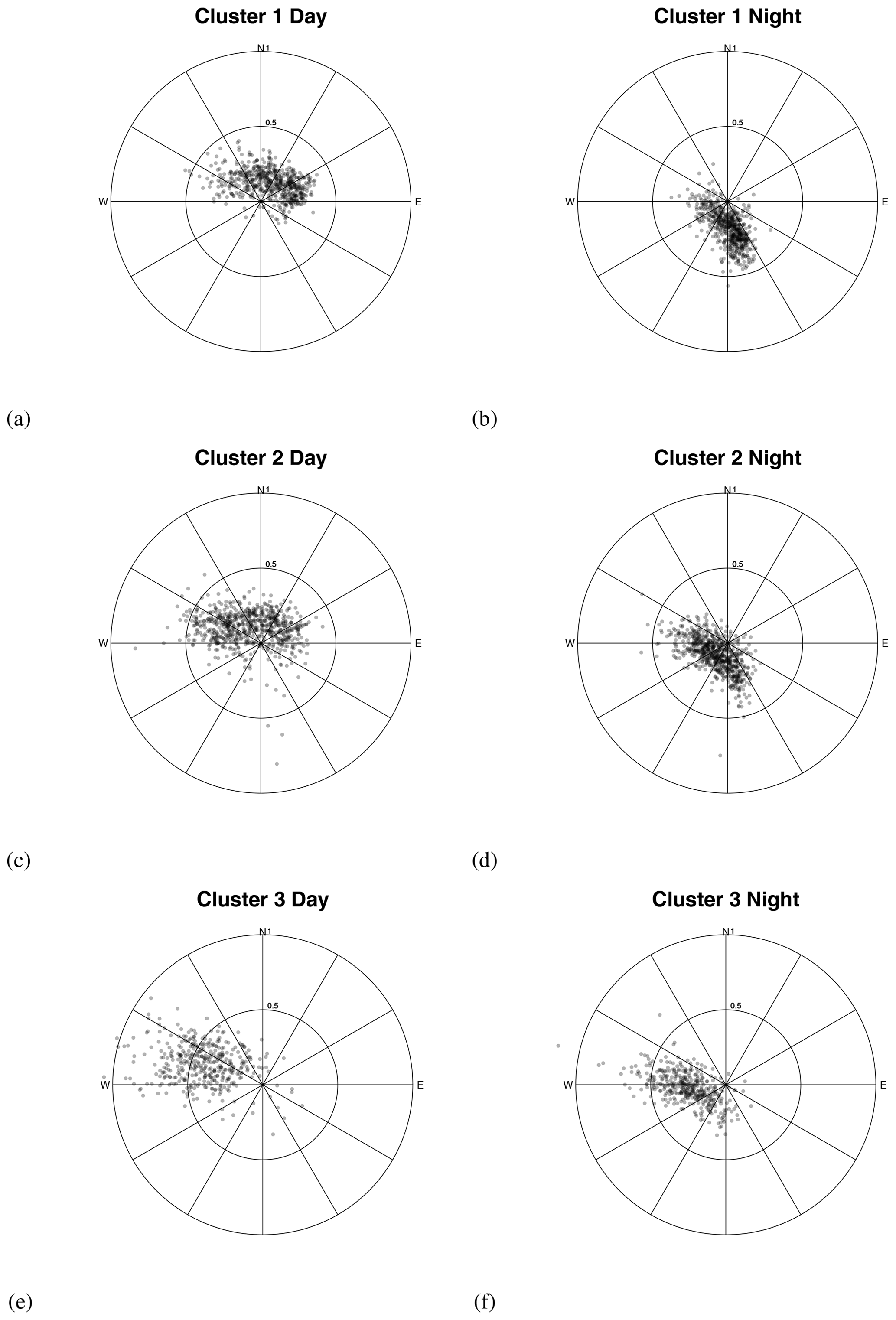
Figure 7 Hodographs of hourly mean surface wind at the CRA (m s⁻¹) for Clusters 1 to 3 during the night (23:00–02:00 UTC; (b), (d), (f)) and the day (11:00–15:00 UTC; (a), (c), (e)).

Lastly, Fig. 7 shows hodographs of hourly surface wind at the CRA for both night and day. Due to the proximity of the Pyrenees, thermally induced circulations are expected on sunny days, with wind blowing from the plain to the mountain in the daytime (northerly sector) and conversely at night (southerly sector). As expected, this alternation of the wind between day and night is most visible in Cluster 1, but it can also bee seen in Cluster 2 and, to a much lesser extent, in Cluster 3. In Cluster 2, strong southerly wind is sometimes observed even in the daytime, again presumably corresponding to foehn events.

3.2.3 Seasonality

Figure 8 shows the occurrence frequency of days in each cluster within the four seasons. Clearly, for all clusters, the frequencies deviate from an equal distribution (25 % of days in each season). This demonstrates the fact that weather regimes have their own seasonality. Cluster 1 has an excess (32 %) of summer days, consistent with the main characteristics (fair-weather anticyclonic days). In the same way, in Cluster 3, 33 % are winter days and only 14 % are summer days, which is consistent with disturbed weather being more frequent in winter and spring. Cluster 2 has a deficit (19 %) of winter days, but no explanation for this is obvious to us.

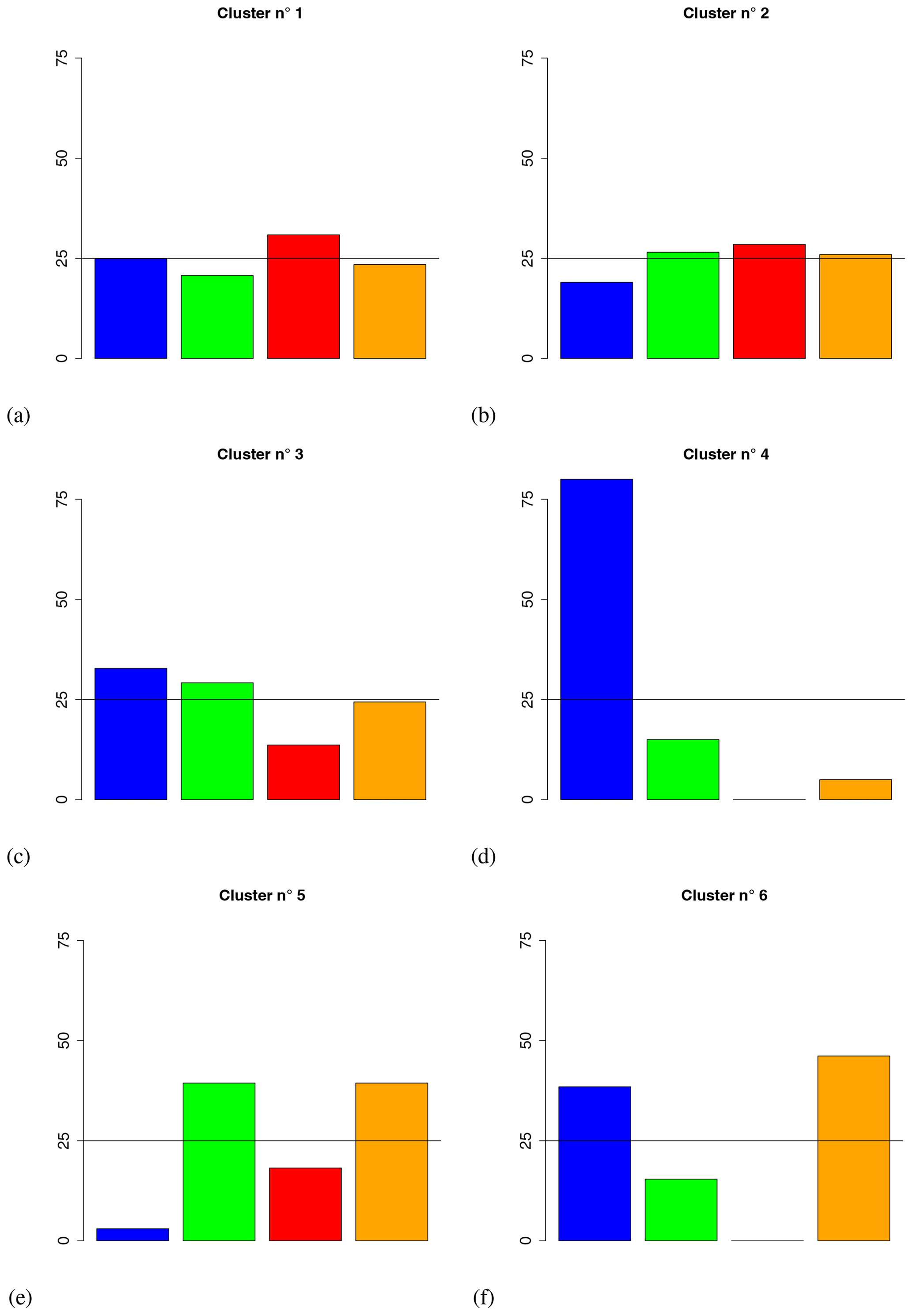
Figure 8 Seasonal occurrence of days in each cluster (each value is the % of all days in the cluster).

3.2.4 Global portrait of the major clusters

To summarize the last three paragraphs, we now attempt to depict the main characteristics of the weather regimes emerging from the three major clusters:

• Cluster 1 is characterized by high-pressure, clear-sky, warm, dry, and weak-wind days, during which thermal surface breezes develop over the Pyrenean foothills. Cluster 1 will subsequently be referred to as “the fair-weather cluster”.

• Cluster 3 will be called “the atmospheric disturbance cluster”, as it is characterized by a sustained north-westerly wind with cold, wet and cloudy conditions.

• Cluster 2 contains days that are characterized by intermediate values for most variables and show similarities with days in either Cluster 1 or 3. Thus, this cluster is much more difficult to portray. Cluster 2 also contains days with characteristics of foehn days that will be investigated later with specific diagnostic tools.

3.3 Analysis of the three minor clusters

3.3.1 Winter windstorms (Cluster 4)

Cluster 4 contains only 20 d but is characterized by extreme values for several variables. It reveals wind patterns similar to Cluster 3, with north-westerlies at altitude (Fig. 5d) but channelled along the Pyrenees (thus from the west) below the crest level (Fig. 6d). However, unlike Cluster 3, Cluster 4 contains only strong-wind days (the speed of the daily averaged wind at 2850 m a.s.l. is between 18 and 35 m s⁻¹, Fig. 5d).

In addition, Cluster 4 has the densest cloud cover of all the clusters (median above 70 %, Fig. 4f), just above Cluster 3. However, these two clusters differ strikingly in terms of temperature anomalies (Fig. 4a and b), with Cluster 4 revealing positive anomalies (i.e. temperatures above the seasonal mean) at both the PDM and the CRA. The seasonality of Cluster 4 is remarkable, with more than 75 % of its days being winter days none in summer. The positive temperature anomaly may be explained by the rapid advection of oceanic air to the CRA, which is warmer than continental air in winter.

We can therefore consider Cluster 4 to be a collection of winter windstorms.

3.3.2 Foehn (Clusters 5 and 6)

Clusters 5 and 6 share similar wind characteristics, with south-westerly winds at 2850 m a.s.l. (Fig. 5e–f) and southerly winds at 1600 m a.s.l. (Fig. 6e–f). The median temperature anomalies at the PDM (Fig. 4a) are similar for both clusters and slightly positive (i.e. the temperature is a bit above the seasonal mean). Comparing Fig. 4a and b shows that for Clusters 1–4, the temperature anomalies are very similar at the PDM and CRA, which is expected given the small distance between the stations (28 km). Strikingly, this is not the case for Cluster 6, where we can see a much higher positive temperature anomaly at the CRA (above +5 ^∘C, the highest median value of all the clusters) than at the PDM (Fig. 4b). This is also true for Cluster 5, but to a lesser extent. Lastly, the relative humidity anomaly is negative for both Clusters 5 and 6 (Fig. 4e).

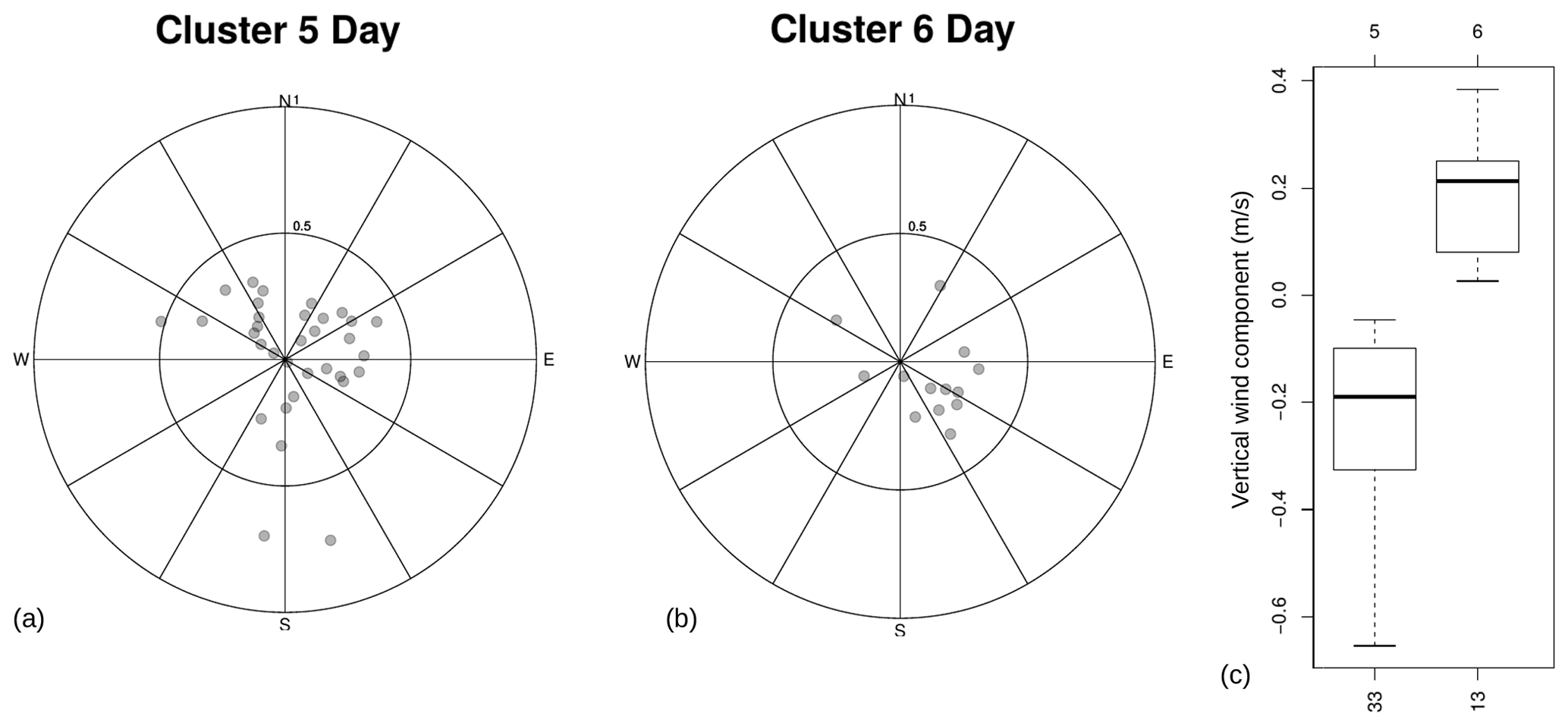
Figure 9 Hodographs of daytime (11:00–15:00 UTC) mean surface wind at the CRA (m s⁻¹) for Cluster 5 (a) and for Cluster 6 (b). Boxplots (c) of the vertical component of the wind (m s⁻¹) measured by the VHF profiler at 2850 m a.s.l. for Clusters 5 and 6.

The south-westerly wind at altitude and southerly wind below the crests, in combination with warmer and drier air at the CRA, strongly suggest that Clusters 5 and 6 correspond to foehn situations. A higher positive temperature anomaly at the CRA is observed in Cluster 6 than in Cluster 5. This further suggests that the foehn effect in Cluster 6 is more penetrative and affects the surface on the lee side more. Figure 9a and b help us to verify this. The observation period of surface wind at the CRA in this figure is restricted to the daytime (otherwise the hodographs show no obvious difference for surface wind when averaged at the full-day scale). North-easterly anabatic breezes can be observed in most cases in Cluster 5 (Fig. 9a), in addition to southerly foehn wind cases, while Cluster 6 (Fig. 9b) almost exclusively shows southerly foehn wind. At night, the southerly katabatic flow combines with the southerly foehn, so there is no clear difference in wind direction between Clusters 5 and 6 (not shown). This occurrence, in the daytime, of surface anabatic breezes under foehn conditions will be discussed later with diagnostic tools for thermally driven circulations.

Finally, we noticed a clear difference between the two clusters in the daily mean of the vertical component of the wind (Fig. 9c). This suggests that this variable played an important role in the clustering when separating those two clusters. A physical interpretation of this difference is discussed below in Sect. 4.4.

The attribution of the days in Clusters 5 and 6 to foehn situations is also in line with the negative pressure anomalies at the PDM (Fig. 4c) because the PDM is downwind of the main Pyrenean crest (Fig. 1). However, this pressure anomaly could also be due, at least partly, to the fact that foehn events often precede the arrival of pressure lows from the Atlantic. The attribution is also consistent with the seasonality of Clusters 5 and 6 (Fig. 8), as the foehn is a phenomenon that mainly occurs in spring and autumn (according to studies conducted in Alpine regions; for example, Bouët (1972) and Richner and Gutermann (2007). We found no literature reference on foehn climatology in the Pyrenees. In the next section, using diagnostic tools specifically built to detect or characterize foehn events, we will check whether other clusters also contain foehn events.

4 Consideration of specific diagnostic tools

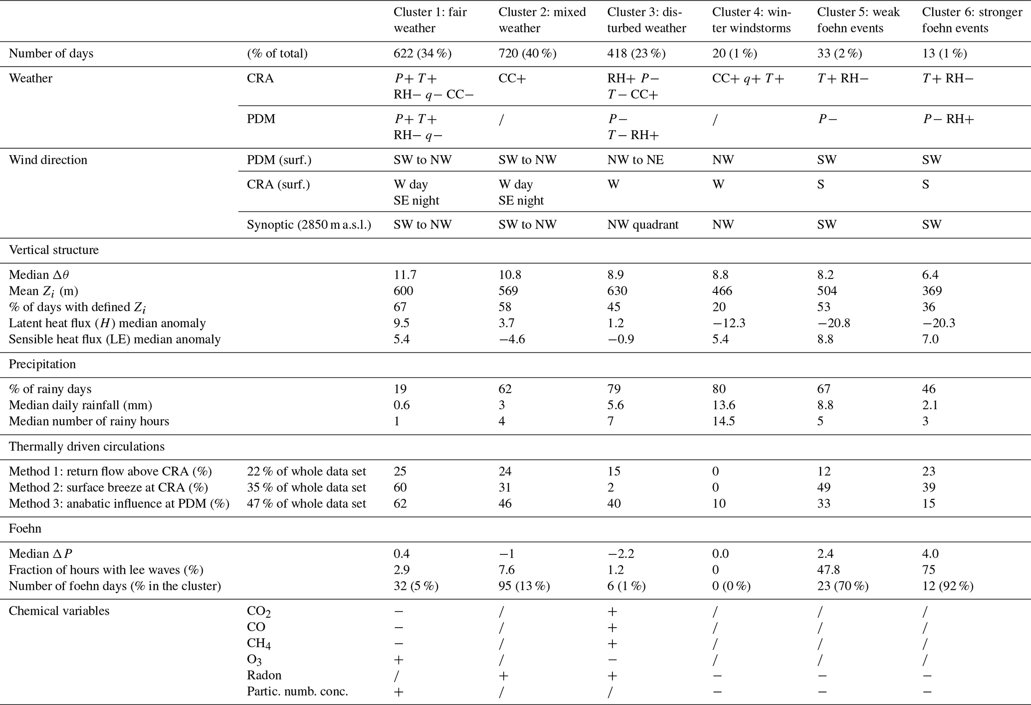
In this section, the diagnostic tools defined in Sect. 2.3 will be applied to the data from each cluster with the aim of refining the analyses conducted above or to validate the conclusions. All the results are summarized in the synthetic Table 4 but are detailed and commented on below.

Table 4 Synthetic table of the results of the study. For all variables in the “Weather” and “Chemical variable” sections, + stands for “above the median of the whole data set”, − stands for “below the median of the whole data set”, and $/$ stands for “close to the median”. For example, in Cluster 1, for CO₂, − means that most of the CO₂ anomaly distribution is lower than the full data-set median. For the “Weather” section, P stands for pressure, T stands for temperature, RH stands for relative humidity, q stands for specific humidity, and CC stands for cloud cover.

4.1 Vertical structure of the atmosphere dynamics

The first two diagnostic tools detailed in Sect. 2.3.1 provide information about the vertical structure of the atmosphere. First, we can see in Fig. 10a that, among the major clusters, the median difference Δθ (equal to θ_PDM−θ_CRA) is the highest for Cluster 1, which indicates the presence of a more stable atmosphere than in Clusters 2 and 3, consistent with fair weather and anticyclonic conditions. Cluster 3 and 4 both have a low Δθ, suggesting a less stable troposphere, which is to be expected in disturbed weather. Finally, we notice that Clusters 5 and 6 also have the lowest Δθ among the six clusters: this will be discussed further in Sect. 4.4.

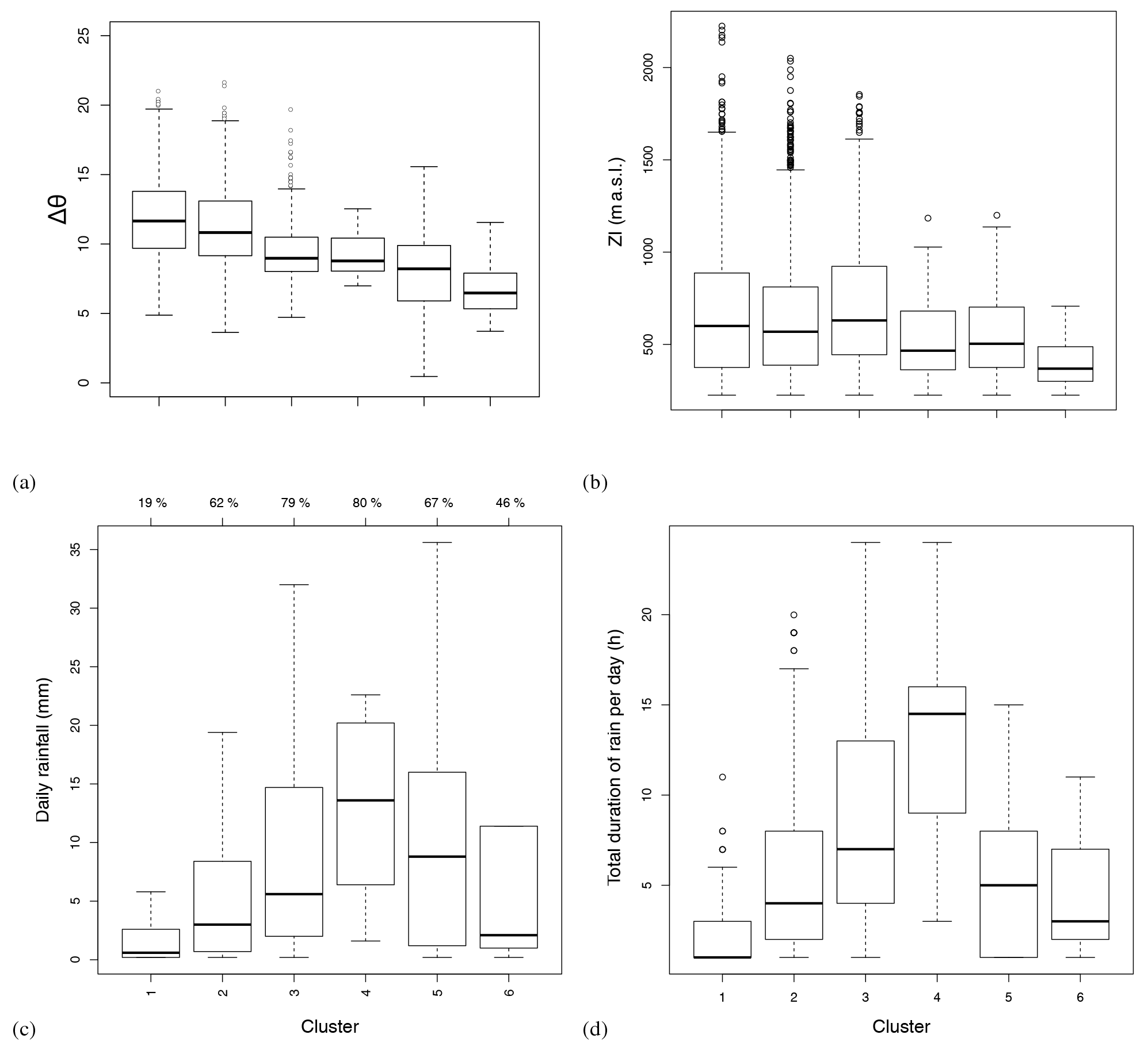
Figure 10 Boxplots of (a) the mean daily difference in potential temperature $\mathrm{\Delta }\mathit{\theta }={\mathit{\theta }}_{\mathrm{PDM}}-{\mathit{\theta }}_{\mathrm{CRA}}$, (b) the convective boundary layer Z_i (from UHF profiler data), (c) the daily rainfall (dry days excluded, in mm), and (d) the number of rainy hours per day (dry days excluded). The top of panel (c) shows the percentage of rainy days in each cluster.

The sensible heat flux H median anomaly is also the highest for Cluster 1 (Table 4), which is consistent with fair weather conditions, as the ground receives a great deal of sunlight which is then transferred into the atmosphere as heat flux. The presence of clouds and rain in Clusters 2 and 3 is less favourable to surface heating and surface convective instability, leading to a smaller positive anomaly in H and a negative anomaly in the latent heat flux LE. The anomaly in H becomes negative in Clusters 4, 5, and 6. In the situation of winter storms (Cluster 4), we saw earlier that the temperature anomaly is positive in this cluster due to the advection of warmer oceanic air. Here, the surface layer is usually stable or dynamically mixed, as clouds and rain prevent dry convection. Sensible heat flux is weak or even negative. In foehn situations, the anomaly in H is also negative because foehn brings warm air to the CRA, which also leads to weaker or even negative sensible heat flux (as the air gets even warmer than the ground). Conversely, the LE anomaly is positive in foehn clusters. In fact, the drier and warmer air of the foehn strongly favours the evaporation of soil moisture. Strong winds in cluster 4 also favour evaporation, although less than in the dry foehn clusters. This could explain the smaller positive anomaly in LE in Cluster 4. A positive anomaly in LE of the same magnitude is found in Cluster 1, but this is associated with the solar heating of the surface.

The distribution of the Z_i estimation (CBL height) within clusters may be affected by how the estimation is made. To get a Z_i estimation of good quality, a well-formed CBL capped by a more stable and laminar atmosphere is needed, which is generally not the case during disturbed weather events. This induces a difference in data availability for Z_i estimations between clusters. By comparing the availability of the UHF wind profiler data and of the estimation, we were able to compute the percentage of days for which the UHF wind profiler data are available but the Z_i is not defined for each cluster. This provides information about the proportion of disturbed days within each class. As expected, among the major clusters, Cluster 3 has the lowest rate of available Z_i estimations (44.7 %; Table 4). However, the boxplot in Fig. 10b shows that the median Z_i values (when available) for the three major clusters are similar, with the difference being inferior to the UHF resolution (75 m). Cluster 4 has the lowest number of available Z_i days (19.8 %), which is consistent with with the assumption of winter wind storms. Comparing the two foehn clusters, Cluster 6 has more unavailable days than Cluster 5 (63.8 % and 47.1 %, respectively). With the assumption made earlier that Cluster 6 contains stronger foehn events, we can assume that the downslope hot wind either prevents the CBL from forming or tends to squeeze it near the ground, typically with a top below (500 m) a.s.l., causing a lower median Z_i in Cluster 6. The smaller Z_i in foehn clusters is also supported by the negative anomaly in H fluxes. With a smaller buoyancy flux at the surface (due to the warm air aloft), CBL growth is significantly reduced.

4.2 Precipitation

In this section, we discuss the occurrence of precipitation in the different clusters based on the diagnostic variables defined in Sect. 2.3.1, starting with the fraction of dry days (days with no rain, Table 4). As expected, the clusters with the most frequent rain occurrence are Clusters 3 and 4 (79 % and 80 % of the days are rainy, respectively), and the least rainy cluster is Cluster 1 (19 % of the days are rainy).

In addition, the rainy days in Cluster 1 are characterized by short episodes (mostly less than 5 h) and small daily amounts (Fig. 10c and d). Outliers in the boxplots of daily amounts of precipitation correspond to the heaviest rain episodes. For clarity, such outliers are not displayed in Fig. 10c but are actually numerous in Clusters 1, 2, and 3. In contrast, there are much fewer long-lasting episodes in these clusters (represented as outliers in Fig. 10d). This suggests that the heaviest rainfalls correspond to convective storms. As expected, the median rainfall and rain duration are the highest in Clusters 3 and 4 – the latter (winter windstorm days) being the one with the highest values.

Comparing the two foehn clusters, Cluster 5 contains more rainy days than Cluster 6, in line with less solar radiation (Fig. 4d), more humidity (Fig. 4e), and a wider range of cloud cover fractions (Fig. 4f). This supports the idea that Cluster 6 is characterized by a more intense foehn, as subsidence causes adiabatic heating (high-temperature anomaly, Fig. 4b), air drying, cloud evaporation, and convection inhibition. Moreover, stormy situations over the Pyrenees are frequently associated with an unstable south-westerly synoptic wind. Thus, foehn situations are often followed by or occur at same time as storms. These situations generally occur generally in summer, which is consistent with Fig. 8, where Cluster 5 contains summer days while Cluster 6 does not. This may explain the higher proportion of rainy days in Cluster 5.

4.3 Thermally driven circulations

The three methods reported by Hulin et al. (2019) were designed to detect thermally induced flows at different scales and locations: (1) the altitude return flow of plain-to-mountain pumping, (2) the surface breeze at the CRA, and (3) the local anabatic influence detected in situ at the PDM (respectively referred to as Methods 1–3). These methods were applied to our data set and the results were analysed by cluster (Fig. 11). The numerical values of detection rates for all clusters and for the whole data set are available in Table 4. The detection rates we found for the complete data set (22 %, 35 %, and 47 % for Methods 1, 2, and 3, respectively) are close to the ones found in Hulin et al. (2019) (27.4 %, 27.5 %, and 47.3 %, respectively), which proves the consistency of the methods.

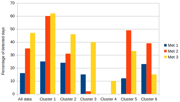
Figure 11 Percentage of days selected by the three methods for all the data set and for the six clusters. In the “All data” group, the percentage is relative to all 1856 observation days. In each cluster, the percentage is relative to the population of the cluster.

Hulin et al. (2019) evidenced that, for a given day in their database, the meteorological conditions did not always meet (or miss) the criteria for all three methods at the same time. They concluded that these different types of thermally induced flows are not systematically concurrent and may occur independently from each other. This may explain why, in our case (Fig. 11), the percentages obtained for a given cluster differ between methods. Nevertheless, all the methods lead to a common hierarchy when the clusters are compared to each other.

Concerning the three major clusters, all three methods agree that anabatic days are most frequent in Cluster 1 and least frequent in Cluster 3. This is consistent with the main characteristics of the clusters depicted in Sect. 3, as thermally driven circulations need a context with low synoptic wind and sufficient solar radiation to develop. These conditions are typical of Cluster 1, partly occur in Cluster 2, and are rare in Cluster 3. We noticed that Method 2 (a breeze at the CRA) is the method that gives that largest discrepancies between Clusters 1 and 3 (60 % and 2 %, respectively). This very low occurrence in Cluster 3 is not surprising considering that strong westerly winds are more frequent in this cluster than in the other two (Figs. 5 and 6), especially close to the surface at the CRA (Fig. 7). Cluster 4, composed of winter windstorms, is also characterized by strong winds (Figs. 5–7), and in line with this, the first two methods detect no anabatic days at all, while method 3 reveals that 90 % of the days have no anabatic influence at the PDM (the remaining 10 % correspond to only 2 d and are likely false detections).

Methods 1 and 3 give fewer occurrences of thermal flows for the foehn clusters (5–6) than Clusters 1–3 (Fig. 11) – except for Cluster 6, where altitude return flows above the CRA are found as frequently as in Clusters 1 and 2. In foehn conditions, sustained southerly or south-westerly wind at the altitude of the Pyrenean summits and subsidence on the lee side of the barrier do not favour the development of thermal flows, or at least flows that reach such a high altitude, which explains the low occurrence rates in Fig. 11. The case of altitude return flows in Cluster 6 is hard to interpret physically, but this result may also be caused by the poor statistical representativeness of Cluster 6 (only 13 d) and the risk of the false detection of a return flow by Method 1 if a short foehn event occurs in the middle of the day. Concerning Method 2, the relatively high occurrence of a surface breeze at the CRA for the foehn clusters (Fig. 11) could be seen as paradoxical in a synoptic context of sustained wind. However, unless the foehn runs deep into the plain, the foothills are often sheltered from the foehn wind. Moreover, clear sky can easily develop in foehn conditions (Fig. 4d). In these conditions, thermal breezes can develop at the surface (as discussed in Sect. 3.3.2) and can be detected by Methods 2 and 3. The proportion is higher in Cluster 5 due to the presence of a deeper foehn in Cluster 6. In these situations, thermally driven winds in valleys and from a plain to a mountain are not incompatible with a foehn event aloft.

Method 3 gives the same hierarchy among Clusters 1–3 as the other methods but shows a significant percentage of anabatic days even for Cluster 3 (40 %), which may be unexpected in disturbed weather conditions. To investigate the local anabatic influence at the PDM, we plotted the mean diurnal cycle of radon for each cluster (Fig. 12). A daytime increase in radon is a clear signature of an anabatic influence at a mountain-summit observatory (Griffiths et al., 2014). No evident diurnal cycle of radon is visible in Fig. 12 for the three minor clusters (4–6) as foehn events and winter windstorms are not favourable conditions for thermal flows to develop close to the PDM summit because there is strong synoptic wind at altitude. Clusters 1–3, in contrast, exhibit clear diurnal cycles with a maximum at 14:00–15:00 UTC and a minimum at night. However, the cycle amplitude is above 1000 mBq m⁻³ for Cluster 1, around 700 mBq m⁻³ for Cluster 2, but much lower (around 300 mBq m⁻³) for Cluster 3. These amplitudes are in line with the hierarchy of anabatic day occurrence among Clusters 1, 2, and 3. Even though the percentage of days with detectable anabatic influence is similar for Clusters 2 and 3, the cycle amplitude in Cluster 2 is twice as large as that in Cluster 3, suggesting that, in Cluster 3, the anabatic influence is notably less than in Cluster 2. This conclusion is consistent with Cluster 3 containing days that were less favourable to a local anabatic influence at the PDM.

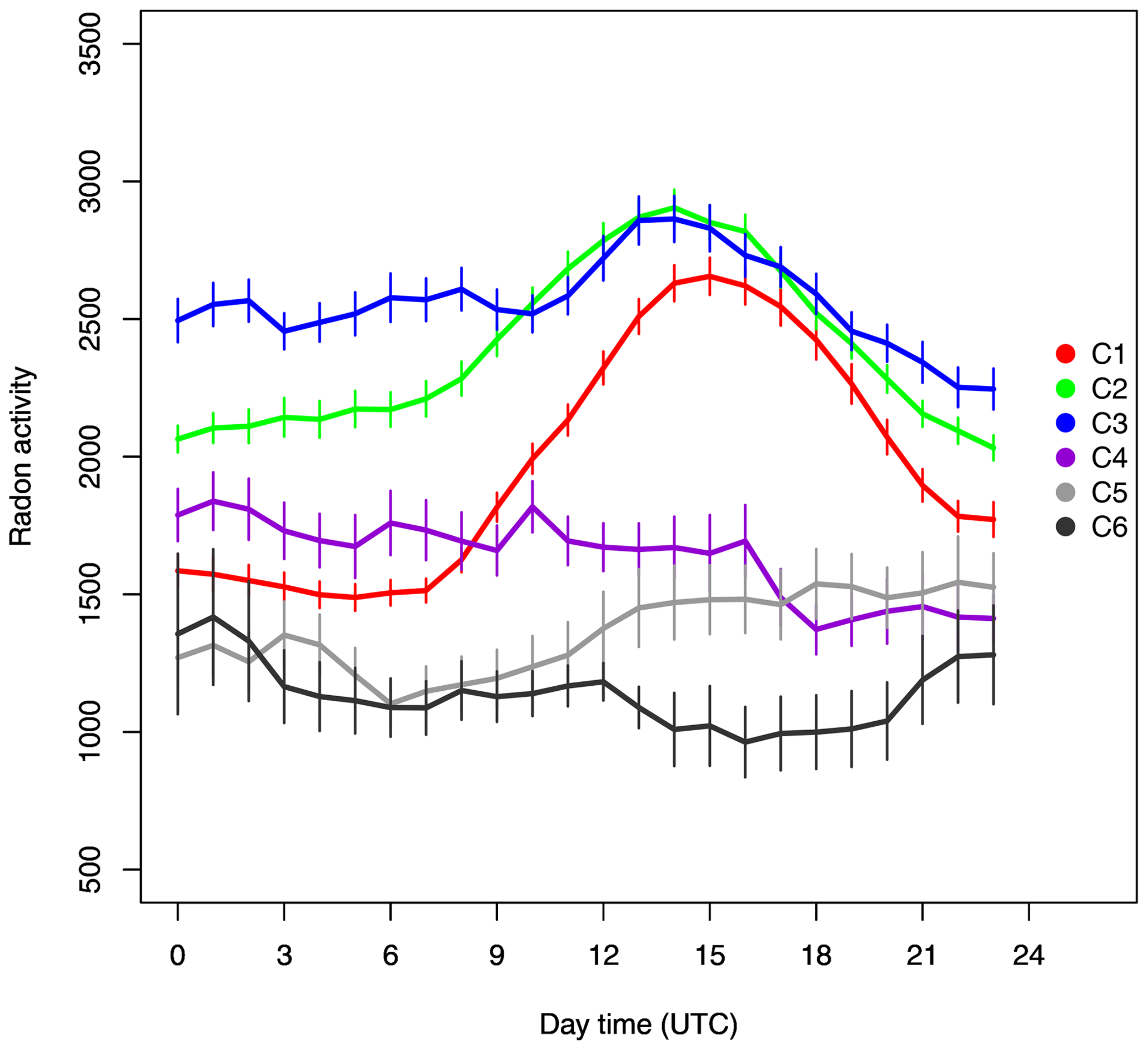
Figure 12 Mean diurnal variation in radon (mBq m⁻³) for each cluster (C1–C6). Vertical segments represent the standard error.

Lastly, Fig. 12 supports the use of specific humidity for implementing Method 3 (as suggested by Griffiths et al., 2014), as the largest radon cycles coincide with the most anabatically influenced days, as seen from a specific humidity point of view.

We can finally conclude that the thermally induced flow occurrences given by the three methods are globally consistent with expectations based on the main meteorological characteristics of the clusters (portrayed in Sect. 3), which are or are not favourable to thermal flow development.

4.4 Foehn

This part will focus on the diagnostic tools that are designed to characterize foehn events, starting with the pressure difference across the Pyrenees (ΔP), defined here as the upstream minus the downstream pressure. Foehn events should thus induce positive ΔP values across the Pyrenees. However, due to the orientation of the main Pyrenean chain, a north–south pressure gradient may also be associated with the westerly component of the geostrophic circulation. A crude estimation shows that 10 m s⁻¹ geostrophic westerlies would be driven by a 1 hPa difference over 100 km, which is the approximate distance between Monzon and the CRA. Consequently, we will consider pressure differences well above 1 hPa to be the signature of foehn events.

The median ΔP in Clusters 5 and 6 are, respectively, 2.4 and 4.0 hPa (Table 4), where Cluster 1 has a median ΔP of 0.4 hPa and all four remaining clusters have negative ΔP (the lowest being Cluster 3, with −2.2 hPa). The negative differences found for Clusters 2 and 3 can be explained by the prevalence of synoptic winds with a northerly component, which will induce a reversed pressure dipole across the chain. Clusters 5 and 6 largely overcome the 1 hPa difference associated with geostrophic westerlies, which is consistent with the hypothesis that foehn events form these clusters. The higher ΔP in Cluster 6 than in Cluster 5 is also consistent with our interpretation of a stronger foehn effect on the lee side (Sect. 3.3.2).

A second diagnostic of foehn events is the presence of lee waves above the CRA that can be detected with the tool described in Sect. 2.3.3. This tool firstly gives the fraction of hourly timestamps flagged as foehn when lee waves are detected (Table 4). As expected, Clusters 5 and 6 have by far the largest fractions among the six clusters (48 % and 75 %, respectively). Focusing on the three major clusters (1–3), foehn events are found most frequently in Cluster 2 (8 %).

Then, a daily index was computed, with a foehn day considered to be a day when a minimum of 6 h were flagged as having a foehn present. The total numbers and fractions of foehn days in the clusters are also presented in Table 4. The daily percentages are found to be systematically higher than the hourly ones due to the fact that short foehn events (6 h) have the same weight as episodes lasting a whole day in the daily flag. Interestingly, in absolute terms, the number of foehn days in Cluster 2 (95) is greater than the number of foehn days in Clusters 5 and 6 (35 d when adding both clusters). These events in Cluster 2 appear in Fig. 5b as the strongest winds in the SW quadrant. This means that the unsupervised clustering used here was not able to gather all foehn days into specific clusters. This could partly be explained by the fact that those days also correspond to a larger daily rainfall relative to the rest of the days in Cluster 2 (not shown). Thus, they correspond to the situation (mentioned in Sect. 1) of unstable south-westerly flows with the occurrence of storms. The very high proportion of foehn days in Clusters 5 and 6 reveals that the most intense foehn events have a characteristic signature in the 23 meteorological variables listed in Table 2. In Cluster 6, one day is not flagged as having a foehn simply because the VHF data point is missing this day. For Cluster 5, 10 d are not flagged as having a foehn, four of which are because of missing data. The remaining 6 d have either a wind that is too westerly to be in the scope of the index or a mean wind that is not strong enough to generate lee waves (Fig. 5e).

The information that Clusters 5 and 6 are composed of days with a significant occurrence of lee waves also provides us with a possible explanation for the difference seen in the boxplots of the vertical component of the wind (Fig. 9c). We can speculate that the difference is due to a horizontal phase shift of the lee waves above the CRA. The boxplots show that Cluster 5 is on average associated with a negative vertical velocity, while Cluster 6 is associated with a positive vertical velocity. This suggests that the positioning of the mountain wave may be different in both situations: during Cluster 6 cases, the CRA is more frequently located in the ascending region, suggesting that the descending region may be closer to the mountain, allowing foehn penetration down to the surface. This specific topic deserves more work (especially numerical modelling).

5 Impact on the atmospheric composition

This section will investigate whether there are statistical differences in the atmospheric composition variables (Table 2, lower list) between clusters, and will discuss what could explain those differences. A question of particular interest is the influence of local and regional transport on the atmospheric composition in the different weather types.

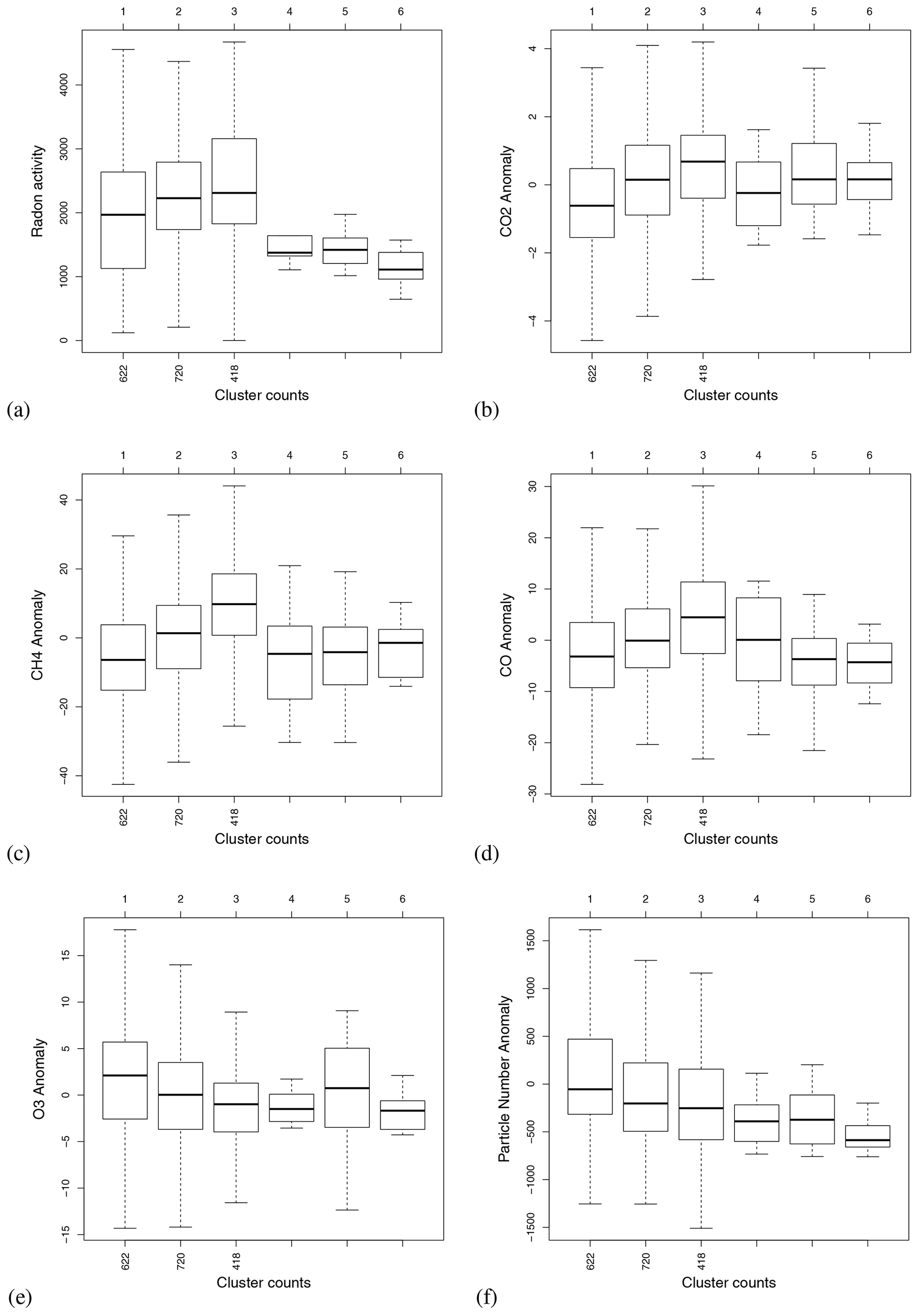
Figure 13 Boxplots of (a) radon volumic activity (mBq m⁻³) and of anomalies in (b) CO₂ (µmol mol⁻¹), (c) CH₄ (nmol mol⁻¹), (d) CO (nmol mol⁻¹), (e) O₃ (nmol mol⁻¹), and (f) particle number concentration (# cm⁻³). All variables were measured in situ at the PDM.

Boxplots of the mole fraction anomalies in CO₂, CO, CH₄, and O₃, the particle number concentration anomaly, and radon activity are displayed by cluster in Fig. 13 and discussed in detail in the next subsections. Before this, a general comment is that the dispersion of values within a given cluster is usually quite large in many cases, revealing the complexity of the physical and chemical processes linking source and receptor regions, even in well-identified weather regimes. Nonetheless, when the clusters are compared for a given variable, in most cases the distributions are sufficiently separated from each other to evidence the true statistical difference between the clusters' means. In the Supplement, we give the p value of the t test computed for each variable and for each couple of clusters.

5.1 Radon as a tracer of continental influence

As radon is constantly emitted from continental surfaces and is only subject to radioactive decay (its half-life is 3.8 d), high radon activity at a mountain observatory like the PDM reveals the transport of air influenced by the European surface (e.g. Griffiths et al., 2014, for the Jungfraujoch). However, it tells us little about the scale of the transport pattern. The transport of continental radon-rich air may occur at a local scale, e.g. driven by anabatic flows in the close mountain area, or at a larger scale if the entire regional low troposphere is subject to vertical mixing, e.g. in convective or frontal conditions. In the latter case, the synoptic horizontal transport may also bring radon-rich air masses to the PDM. On the contrary, in stable anticyclonic conditions, vertical mixing tends to be inhibited, and the regional troposphere is expected to be radon depleted at the altitude of the summits.

The median volume activity of radon (equivalent to the molar concentration¹) is found to be lower, medium, and higher in the major Clusters 1, 2, and 3, respectively.

From a radon point of view, the fair weather conditions that prevail in Cluster 1 are thus equivocal: on the one hand, atmospheric stability should generate a regional context of low radon activity in the free troposphere around the PDM; on the other hand, an anabatic influence should be favoured in fair weather conditions (Fig. 12). The boxplots for radon in Fig. 13a resolve this inconsistency to some extent: despite a wide distribution of radon values in Cluster 1, the median is the lowest among the major clusters, suggesting that in the majority of cases, the daily mean radon concentrations at PDM seem to be dominantly influenced by the regional context compared to daytime anabatic transport. Figure 12 further supports this statement. The nighttime free-tropospheric radon background in Cluster 1 is much lower than that in Clusters 2 and 3, and even the large amplitude cycle is not sufficient to raise the radon activity above that in Clusters 2 and 3 at the time of the afternoon maximum. The daily mean will thus clearly be lower in Cluster 1 (and the highest in Cluster 3).

Looking at Cluster 4, the mean/median radon values are low (around 1300 mBq m⁻³, Figs. 12 and 13a). We can speculate that during north-westerly windstorms, there is rapid advection of radon-poor oceanic air to the PDM with limited mixing with the continental boundary layer, but a backward particle dispersion analysis would be needed to support this.

Interestingly, the radon values are the lowest for the foehn Clusters 5 and 6. Again a backtrajectography study is needed to explain this observation, but, so far, two (not mutually exclusive) assumptions can be made: (i) during their transport to the PDM, the airmasses avoid flying over the western part of the Iberian Peninsula, a hot spot of radon emissions in Europe (see e.g. the exhalation maps in Quérel et al., 2022) (it should be noted that such an explanation could also be valid for the low values in Cluster 4); (ii) during foehn episodes, the PDM is located in the lee of the Pyrenean crest and thus in the subsident part of the foehn wave, which brings radon-poor air from aloft to the station. In any case, the low radon values in foehn conditions clearly deserve more investigation.

5.2 Other gases and particles in the major clusters

The hierarchy found for radon among the three major clusters (1–3) (Fig. 13a) is also valid for the anomalies in CO₂, CH₄, and CO – namely, the median value is negative in Cluster 1, near zero in Cluster 2, and positive in Cluster 3 (Fig. 13b–d). The ozone and particle number anomalies display a reversed pattern – i.e. high values for Cluster 1 and low values for Cluster 3 (Fig. 13e–f).

As CO₂, CH₄, and CO are primary pollutants that are mostly emitted from the surface (as is radon), the interpretations given for radon in Sect. 5.1 may be also valid for them. However, they have specific atmospheric sinks that should be considered.

Photosynthesis is the main sink of tropospheric CO₂ (Necki et al., 2003; Lin et al., 2017). The fair-weather days in Cluster 1 appeared to be warmer and to benefit from greater solar irradiance than those in the other major clusters (Fig. 4a, b, and d). We can presume that, under such conditions, the photosynthetic activity was higher at the regional scale and could contribute to the observed CO₂ depletion. Note that the anabatic influence (favoured in Cluster 1) can further contribute to the depletion in the CO₂ daily mean, as the CO₂ diurnal cycle at the PDM shows a daytime minimum caused by the local photosynthetic activity (Hulin et al., 2019).

For CO and CH₄, low anomalies in Cluster 1 could be due to a depletion in gas concentration at the regional scale due to enhanced oxidation by the hydroxyl radical (OH), which is produced in the troposphere by the photolysis of water vapour (Seinfeld and Pandis, 2016). OH is a common sink of CO and CH₄ in the troposphere (Necki et al., 2003), especially in warm conditions with high solar irradiance. In contrast, in Cluster 3, containing cloudy and cold days, the atmospheric oxidative capacity is lower.

Inversely to radon, the mean tropospheric ozone profile shows a rapid increase with height in the lowest kilometres (Chevalier et al., 2007; Petetin et al., 2018). The elements invoked to interpret the relative radon levels in Clusters 1–3 are again valid for ozone but in the opposite way: enhanced atmospheric stability and the free tropospheric influence may explain the higher ozone levels encountered in Cluster 1; enhanced mixing of the lower troposphere completed by regional horizontal transport to the PDM may explain the lower ozone levels in Cluster 3. Note also that anabatic transport brings ozone-depleted air to the PDM (Hulin et al., 2019), but, as for radon, this antagonistic effect does not obviously dominate over the free tropospheric influence in Cluster 1. High ozone levels in the regional free troposphere can also be reinforced by enhanced photoproduction in Cluster 1 (Fig. 4d).

Concerning the particle number concentration, the increased free-tropospheric influence in Cluster 1 would make us expect cleaner conditions, and thus lower concentration anomalies, than in boundary-layer-influenced cases (Cluster 3). But, interestingly, the opposite is observed, as concentration anomalies tend to be the highest in Cluster 1 (Fig. 4f). To explain this, we can hypothesize that fair-weather days enhance the production of small aerosols by nucleation. An alternative explanation is that anabatic transport, which is favoured in Cluster 1, may have a major influence on the daily averaged concentrations. Indeed, Hulin et al. (2019) showed (in their Fig. 13e) that particle number concentrations may be raised by a factor of 3–4 in the afternoon compared to the nocturnal background during anabatic days. This diurnal evolution of particle number concentration may be linked to the uplift of particles from sources in the valleys. But new particle formation is also favoured during such days, and both explanations (nucleation and anabatic uplift) are not mutually exclusive, since nucleation may occur in the free troposphere as well as in the valleys. Anyway, a deeper analysis of the aerosols at the PDM with appropriate instrumentation (especially a scanning mobility particle sizer) is needed to investigate this question.

5.3 Other gases and particles in the minor clusters

Focusing on Cluster 4, the median anomalies are also negative for all gases and particles (Fig. 13b–f) and are accompanied by low radon levels (Fig. 13a). The assumption of rapid advection of baseline oceanic air to the PDM, invoked for radon in Sect. 5.1, is also consistent for these other variables. Moreover, strong wind conditions favour atmospheric dispersion and dilution.

For the foehn clusters (5 and 6), we do not notice any influence on CO₂ (the anomaly is close to zero, Fig. 13b); however, for the five other variables (including radon), the medians are negative and below the medians of the three major clusters (except O₃ in Cluster 5). The second assumption made in Sect. 5.1 to explain low radon levels (i.e. that the PDM is located in the subsident part of the foehn) seems to be applicable to CO, CH₄, and particles as well, as the levels of these variables are expected to be lower in the free troposphere than in the boundary layer. As CO₂ has a much longer lifetime, it is well mixed in the troposphere. Positive CO₂ anomalies can only be observed very close to sources; they are rarely seen in the free troposphere. Therefore, it is not surprising to see that there is no influence of the foehn on CO₂. On the contrary, O₃ is expected to occur at higher concentrations in subsident air masses. This is, to some extent, the case for Cluster 5 (with large scatter, however), but not for Cluster 6. Further investigation of the origin and transport patterns of air masses in Cluster 6 would be needed to explain those unexpected low ozone levels.

As foehn episodes correspond to south and south-westerly synoptic flows, they can be associated with dust transport from the Sahara and, in turn, enhanced particle number concentrations at the PDM. Surprisingly, this is not found in the distributions of Clusters 5 and 6 (Fig. 13f), where even the 75th-percentile values are low. Again, a trajectory analysis would be needed to determine the source region of the air masses for these two clusters. Further checking is required to ascertain whether dust episodes can be found in the foehn days characterized in Cluster 2 (see Sect. 4.4).

6 Final discussions

6.1 Summary

The present study proposes a non-supervised classification of a basic set of meteorological observation data covering 5 years and collected at both sites of the P2OA, where the CRA is at a foothill site and the PDM is at a mountaintop site. Prior to this study, the diurnal and seasonal components of the time series, as well as the multi-year trends (when present), were filtered out in order to isolate the day-to-day weather changes. The aim of this preprocessing and the subsequent classification was thus to form clusters of observation days with contrasting characteristics of the local meteorology, which could be related to synoptic weather regimes. Then, the statistical distributions of not only those data but also secondary diagnostic data tools derived from the basic data set or complementary observations as well as atmospheric composition data at the PDM were analysed by cluster.

The classification method used was hierarchical clustering computed with the complete linkage method. It resulted in three major clusters (numbered 1–3) and three minor clusters (4–6). All the results are summarized in Table 4, which helps us to draw a global portrait of each cluster as follows:

• Cluster 1 (34 % of the data collection) contains warm, dry, clear-sky days with weak to moderate wind in the free troposphere. Diagnostic tools that are designed to detect anabatic effects confirm that the meteorological conditions in this cluster are the most favourable for the development of regional thermally driven circulations and an anabatic influence at the PDM (Table 4). This cluster is the one with the highest proportion of summer days. This cluster was thus referred to as the “fair-weather cluster”. Under these conditions, low concentrations (relative to the seasonal mean) are found for radon, CO₂, CH₄, and CO, but high concentrations are found for ozone and total suspended particles.

• Cluster 3 (23 %) contains cold, wet, and cloudy conditions with prevailing north-westerlies in the free troposphere. It contains fewer summer days and more winter and spring days than an even distribution. This cluster is the rainiest among the three major clusters (79 % of the days are rainy). Diagnostic tools that are designed to characterize the vertical structure of the lowest kilometres of the atmosphere indicate that Cluster 3 contains the least stable conditions among the three major clusters (the lowest median Δθ) and the lowest percentage of days with a detectable boundary-layer top (only 45 % with a well-defined Z_i) which suggest instability throughout the whole troposphere. This cluster was thus referred to as the “atmospheric-disturbance cluster”. In contrast to Cluster 1, high concentrations are found of radon, CO₂, CH₄ and CO, but low levels of ozone and total suspended particles.

• Cluster 2 (40 %) is to some extent intermediate between Clusters 1 and 3, as it contains various types of situations, some similar to Cluster 1 and others to Cluster 3. Day occurrences are evenly distributed among seasons (there are fewer winter days, nonetheless). But, notably, Cluster 2 contains 95 d detected as foehn days by the diagnostic tool specifically designed to detect lee waves above the CRA in the case of a sustained south-to-south-westerly synoptic wind (Sect. 4.4). The concentrations of all composition variables are found to lie at intermediate levels compared to Clusters 1 and 3.

• Cluster 4 (1 %) is composed of only 20 winter days but has very marked characteristics: strong north-westerly winds, the highest median daily rainfall (13.6 mm of rain, well above the 5.6 mm for Cluster 3), and the highest median number of rainy hours in the collection (14.5 h; it is 7 h for Cluster 3). Rapid advection of oceanic air may explain the high temperature relative to the seasonal mean as well as the low concentrations for all atmospheric species. This cluster was referred to as the “winter-windstorm cluster”.

• Clusters 5 and 6 (2 % and 1 %, respectively) have clear characteristics of south foehn days: a sustained south-to-southerly wind in the free troposphere, hot and dry air on the lee side, and a pressure dipole across the Pyrenees (it has the highest median ΔP of all the clusters). The lee-wave detection tool above the CRA confirms that 70 % and 92 % of the days have lee waves in Clusters 5 and 6, respectively. In addition, the two clusters show a significant difference from the other clusters in terms of heat flux anomalies, including a positive anomaly in the latent heat flux LE and a negative anomaly in the sensible heat flux H, consistent with the advection of warm, dry air to the CRA. The two clusters differ in the intensity of the foehn effect on the lee side. The results suggest that the foehn in Cluster 6 plunges deeper on the lee side than that in Cluster 5, which is supported by the higher temperature anomaly at the CRA (Fig. 4b), the higher median ΔP (Table 4), and more inhibition of the diurnal surface breeze at the CRA (39 % of the days had a surface breeze in Cluster 6, but this value was 49 % for Cluster 5; Table 4). The days mostly come from the spring and autumn in Cluster 5 and from the autumn and winter in Cluster 6. While the foehn has no obvious influence on the CO₂ at the PDM, median concentrations under foehn conditions are found to be low for radon, CH₄, CO, and particles and high for ozone (but only in Cluster 5).

Weather-regime-dependent concentrations have thus been found for the atmospheric species measured at the PDM, and tentative pieces of interpretation have been provided. A comparison of radon levels between Clusters 1 and 3 suggests that the regional free-tropospheric background has a dominant influence on daily averaged concentrations, prevailing over the daytime anabatic influence. This may explain why, when photosynthesis and photochemistry are especially active at the regional scale (Cluster 1), concentrations are concurrently found to be low for CO₂, CH₄, and CO and high for ozone and particles (assuming that new particle formation is enhanced in that case, which is speculative and still to be confirmed by observations). In Cluster 4, all six composition variables have negative anomalies, presumably due to the rapid advection of oceanic air to the PDM. Finally, for the foehn Clusters 5 and 6, we presume that foehn conditions mostly bring higher free tropospheric air to PDM, possibly as the result of transport in the subsident part of the foehn wave downstream of the main Pyrenean crest. However, some results remain unexpected (less ozone in Cluster 6 than 5; no evidence of transported Saharan dust), and tracking the air masses back to their source region remains necessary to get a consistent interpretation for all species.

6.2 Discussion

This non-supervised approach, which requires no external data and no a priori knowledge of the local meteorology, could thus be easily carried out at other observation sites. A question that may arise, however, is whether the approach would be as fruitful at sites with fewer meteorological observations, especially in the absence of observed wind profiles. Further study could involve conducting sensitivity tests with our data set in order to check the robustness of the obtained meteorological regimes when some of the observations are removed (e.g. keeping only near-surface wind data, which are much more widespread than wind profile data). Once it has proven robust for a few-year data set in the absence of wind profiles, one application of this approach could be to study the development of the regimes at the P2OA over a longer period in order to detect the impact of climate change on the occurrence and nature of weather regimes.

As it is a non-supervised approach, however, hierarchical clustering may have limited ability to isolate specific phenomena that are known about a priori. An illustration of this in our study is provided by foehn, because most lee-wave events were found in Cluster 2, which was not specific to foehn. In order to make these foehn events fall into the specific foehn Clusters 5 or 6, one could try to modify the metrics used to compute distances between the data points, giving more weight to variables known to be linked to foehn (the southerly wind component, for example). One could also add the output data from the dedicated diagnostic tools (e.g. the binary lee-wave index or the cross-mountain pressure difference) to the list of variables driving the clustering. This would, at least partly, violate the spirit of a non-supervised approach, but sensitivity tests would nevertheless be interesting to conduct. A purely diagnostic and conditional parametric approach would be complementary to the non-supervised approach.

Finally, adding another perspective, backtrajectography, would bring valuable information about the origin of air masses in the different clusters (4, 5, and 6 in particular). This is needed in order to validate the interpretations proposed above and elucidate those results which remained unexplained.

6.3 Conclusion

When applied to a basic set of preprocessed meteorological data, hierarchical clustering provided ensembles of days where the different variables are consistent with the expected weather types. No contradictory information emerged between variables within a given cluster or between clusters. The diagnostic data products did not contradict – on the contrary, they brought further support to – the links established between the clusters and synoptic weather regimes, especially regarding the foehn clusters, and they allowed us to paint more consistent and comprehensive portraits of the clusters. Hence, we can conclude that hierarchical clustering of the local meteorological data may be a valid and simple approach to characterizing the meteorology of an atmospheric observatory – even in complex terrain – and its influence on the in situ atmospheric composition.