Large-eddy-model closure and simulation of turbulent flux patterns over oasis surface

Large-eddy simulations (LESs) have been increasingly used for studying atmosphere and land surface interactions over heterogeneous areas. However, parameterizations based on Monin–Obukhov Similarity Theory (MOST) often violate the basic assumptions of the very theory, generate inconsistencies with the LES turbulence closures, and produce surface flux estimates depending on LES model resolutions. Here, we propose a novel scheme for turbulent flux estimates in LES models. It computes the fluxes locally using the LES subgrid closure, which is then constrained on the macroscopic scale using MOST. Compared with several other schemes, the new scheme performs better for the various types of land surfaces tested. We validate our scheme by comparing surface flux estimates with field measurements obtained over an oasis surface at various height levels. Additionally, we scrutinize other quantities related to the surface energy balance, including net radiation, ground heat flux, and surface skin temperature, all of which align well with observational data. Our sensitivity experiments, focusing on model horizontal resolution, underscore the robustness of our scheme, as it maintains its corrective efficacy despite changes in horizontal grid spacing. We find that the macroscopic constraint imposed by MOST on LES-estimated fluxes strengthens as the horizontal grid spacing decreases, with a more pronounced influence on sensible than latent heat fluxes. These findings collectively highlight the promise and adaptability of our scheme for improved surface flux estimates in LES models.

1 Introduction

Surface fluxes characterize the exchanges of energy, mass, and momentum between the surface and atmosphere and serve as the lower boundary conditions for atmospheric model simulations. How to estimate the fluxes is a central task of land surface models (LSMs) (Oleson et al., 2007). In almost all existing LSMs, they are parameterized via a network of aerodynamic resistances estimated using Monin–Obukhov Similarity Theory (MOST) (Monin and Obukhov, 1954) which assumes the atmospheric boundary layer to be stationary and horizontally homogeneous.

In recent years, large-eddy-simulation (LES) models have been developed and become a powerful tool for studying land surface and atmosphere interactions over homogeneous and heterogeneous areas. In current LES models (e.g., Deardorff, 1978; Moeng, 1984; Sullivan et al., 1994), turbulence is divided into grid-resolved large eddies and subgrid small eddies. The effects of subgrid eddies are represented by subgrid closures (e.g., Smagorinsky, 1963; Deardorff, 1980; Holt and Raman, 1988). Early LES models are not coupled with LSMs; instead, land surface forcing is prescribed (e.g., Maronga and Raasch, 2013). In recent years, LES models coupled with LSMs have been widely used to study atmospheric turbulence over idealized (e.g., Patton et al., 2005) and natural (e.g., Huang and Margulis, 2010; Shao et al., 2013) heterogeneous surfaces. Estimating surface fluxes for LES models is usually also based on MOST. However, the near-surface diffusivity and viscosity estimated by the MOST-based schemes often diverge from those derived from LES subgrid closures, causing inconsistencies between them (Redelsperger et al., 2001).

To deal with this inconsistency problem in LES models, a strategy is proposed by Shao et al. (2013) to estimate surface fluxes based on the subgrid closure. This strategy ensures that the surface flux estimates and subgrid closure are on a consistent physical basis. However, this requires an extrapolation of eddy diffusivity and viscosity to the surface and thus local surface parameters (e.g., local roughness length), and it is not clear whether the surface fluxes estimated this way satisfy MOST on the scale for which the theory works well.

The problem of inconsistency between subgrid closure and MOST in LES models has been studied by Sullivan et al. (1994). Instead of abandoning the use of MOST, the latter authors proposed a two-part (a turbulent (large-eddy) part and a mean-flow part) subgrid-scale (SGS) eddy viscosity model to achieve better agreement between LES and MOST similarity forms in the surface layer. In their model, the usual SGS turbulent kinetic energy (TKE) formulation for the SGS eddy viscosity is preserved, but a contribution from the mean flow is explicitly included, and that from the turbulent part is reduced near the surface. Sullivan et al. (1994) reported that their model yielded increased fluctuation amplitudes near the surface and better correspondence with similarity forms in the surface layer. While the two-part eddy viscosity model provides an interesting approach to aligning SGS in LESs with MOST, it did not explicitly provide a solution for surface flux estimates in LES models. A questionable assumption of their model is the reduced contribution of the turbulent (large-eddy) part and increased contribution of the mean part to the subgrid eddy viscosity near the surface because this assumption reduces the importance of large eddies which may arise due to surface heterogeneity and thus does not preserve the flux patterns, although the mean values of the flux (in their case, surface shear stress) may be preserved.

This study presents a novel approach to surface flux calculation for LES models. This approach comprises two components. First, it calculates LES subgrid fluxes using the eddy viscosity and diffusivity estimates derived from the LES closure without invoking MOST while considering local turbulence characteristics. Second, it employs a macroscopic constraint to ensure that fluxes averaged over the LES domain, corresponding to scales suitable for MOST applications, align with the MOST principles. This scheme requires only LES-simulated variables, effectively addresses the previously mentioned limitations, and ensures that LES flux estimates are independent of model resolution. It facilitates the knowledge transfer from LES to Reynolds-averaged Navier–Stokes (RANS) models. To evaluate the performance of the new scheme, we select the Heihe Watershed Allied Telemetry Experimental Research (HiWATER; Li et al., 2013) site in Zhangye (38.83–38.92^∘ N, 100.31–100.42^∘ E; 1556.00–1559.00 m above sea level (a.s.l.)) as the focal point. Additionally, we examine several other existing schemes for comparative analysis.

2 New surface flux scheme for LES models

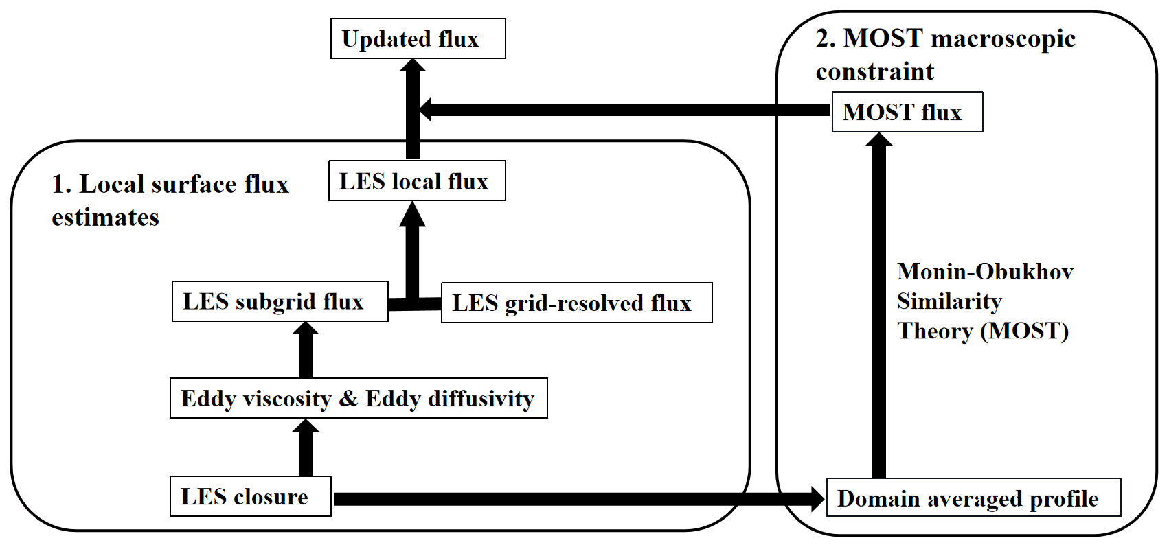
The new scheme, denoted as the MOST-r scheme, is composed of two components. First, surface fluxes are locally estimated, here using the 1.5-order TKE closure (Deardorff, 1980) without invoking the MOST similarity functions in LES. Second, we implement a macroscopic constraint by applying the MOST principles to the LES-simulated fluxes (Fig. 1). For the development and validation of this scheme, we have opted for the Weather Research and Forecast (WRF) LES model. Additionally, we have chosen the 1.5-order TKE closure as the LES subgrid closure.

Figure 1 Schematic diagram of the MOST-r scheme.

2.1 Local surface flux estimates

In LES models, a flux encompasses the contributions from grid-resolved and subgrid eddies, such as sensible and latent heat fluxes, H_les and LE_les,

$$\begin{array}{}\text{(1)}& {\displaystyle }{H}_{\mathrm{les}}=H_{\mathrm{les},\mathrm{g}}+H_{\mathrm{les},\mathrm{sg}},\text{(2)}& {\displaystyle }L{E}_{\mathrm{les}}=L{E}_{\mathrm{les},\mathrm{g}}+L{E}_{\mathrm{les},\mathrm{sg}},\end{array}$$

where H_les,g and LE_les,g are grid-resolved fluxes derived from the LES-simulated vertical velocity $\stackrel{\mathrm{̃}}{w}$, temperature $\stackrel{\mathrm{̃}}{T}$, and specific humidity $\stackrel{\mathrm{̃}}{q}$, i.e.,

$$\begin{array}{}\text{(3)}& {\displaystyle }{H}_{\mathrm{les},\mathrm{g}}=\mathit{\rho }{c}_{\mathrm{p}}\stackrel{\mathrm{̃}}{w}\stackrel{\mathrm{̃}}{T},\text{(4)}& {\displaystyle }L{E}_{\mathrm{les},\mathrm{g}}=\mathit{\rho }L\stackrel{\mathrm{̃}}{w}\stackrel{\mathrm{̃}}{q},\end{array}$$

where ρ is air density, L is latent heat coefficient, and c_p is specific heat capacity at constant pressure. At the surface, due to the boundary condition, $\stackrel{\mathrm{̃}}{w}=\mathrm{0}$; both H_les,g and E_les,g are equal to zero; and thus $H_{\mathrm{les}}=H_{\mathrm{les},\mathrm{sg}}$ and $L{E}_{\mathrm{les}}=L{E}_{\mathrm{les},\mathrm{sg}}$ are conventionally obtained using a LSM, subject to the surface energy and water balance equations, i.e.,

$$\begin{array}{}\text{(5)}& {\displaystyle }{R}_{\mathrm{n}}-H_{\mathrm{les}}-L{E}_{\mathrm{les}}-G=\mathrm{0},\text{(6)}& {\displaystyle }P-E_{\mathrm{les}}-I-R_{\mathrm{0}}=\mathrm{0},\end{array}$$

where R_n is net radiation, G ground heat flux, P precipitation, I infiltration, and R₀ surface runoff. The subgrid fluxes at the surface are parameterized, typically employing the aerodynamic resistance approach,

$$\begin{array}{}\text{(7)}& {\displaystyle }{H}_{\mathrm{les},\mathrm{sg}}=-\mathit{\rho }{C}_{\mathrm{p}}{\displaystyle \frac{\left({\stackrel{\mathrm{̃}}{T}}_{\mathrm{a}}-{\stackrel{\mathrm{̃}}{T}}_{\mathrm{0}}\right)}{r_{\mathrm{h},\mathrm{sg}}}},\text{(8)}& {\displaystyle }L{E}_{\mathrm{les},\mathrm{sg}}=-\mathit{\rho }L\mathit{\beta }{\displaystyle \frac{\left({\stackrel{\mathrm{̃}}{q}}_{\mathrm{a}}-q_{\mathrm{s}}\left({\stackrel{\mathrm{̃}}{T}}_{\mathrm{0}}\right)\right)}{r_{\mathrm{q},\mathrm{sg}}}},\end{array}$$

where ${\stackrel{\mathrm{̃}}{T}}_{\mathrm{a}}$ and ${\stackrel{\mathrm{̃}}{q}}_{\mathrm{a}}$ are air temperature and specific humidity at the lowest model layer, respectively; ${\stackrel{\mathrm{̃}}{T}}_{\mathrm{0}}$ is surface temperature and $q_{\mathrm{s}}\left({\stackrel{\mathrm{̃}}{T}}_{\mathrm{0}}\right)$ saturation specific humidity at ${\stackrel{\mathrm{̃}}{T}}_{\mathrm{0}}$; the parameter β can be expressed as a function of the topsoil moisture (e.g., Irannejad and Shao, 1998); and r_h,sg and r_q,sg are aerodynamic resistances for heat and water vapor, respectively, commonly estimated using the MOST similarity functions which, however, are not directly applicable to problems at the scale of LES.

On the other hand, subgrid eddy viscosity K_m,sg and diffusivity (e.g., for heat) K_h,sg can be estimated via the LES turbulence closure. For a 1.5-order TKE closure, for example, K_m,sg is expressed as

$$\begin{array}{}\text{(9)}& K_{\mathrm{m},\mathrm{sg}}=C_{k}l\sqrt{e},\end{array}$$

where e is the subgrid TKE, obtained by solving the TKE equation in the LES model, and C_k is an empirical parameter of about 0.15. The mixing length l is commonly set to the LES model grid resolution Δ. The subgrid eddy diffusivity can be expressed as

$$\begin{array}{}\text{(10)}& K_{\mathrm{h},\mathrm{sg}}=K_{\mathrm{m},\mathrm{sg}}{\mathit{Pr}}^{-\mathrm{1}},\end{array}$$

where Pr is the Prandtl number, about 0.3.

The eddy diffusivity can be, in turn, used to estimate the aerodynamic resistance, e.g.,

$$\begin{array}{}\text{(11)}& r_{\mathrm{h},\mathrm{sg}}={\int }_{z_{\mathrm{0}\mathrm{s}}}^{z_{\mathrm{1}}}{K}_{\mathrm{h},\mathrm{sg}}^{-\mathrm{1}}\left(z\right)\mathrm{d}z,\end{array}$$

where z_0 s is the aerodynamic roughness affected by the local characteristics of the land surface, and z₁ is the height of the lowest model layer. It is plausible to assume that

$$\begin{array}{}\text{(12)}& K_{\mathrm{h},\mathrm{sg}}\left(z\right)=K_{\mathrm{h},\mathrm{sg}}\left(z_{\mathrm{1}}\right){\left({\displaystyle \frac{z}{z_{\mathrm{1}}}}\right)}^{\mathrm{n}},\end{array}$$

where K_h,sg(z₁) is the subgrid eddy diffusivity at z₁. Then, for n=1, we have

$$\begin{array}{}\text{(13)}& r_{\mathrm{h},\mathrm{sg}}={\displaystyle \frac{z_{\mathrm{1}}}{K_{\mathrm{h},\mathrm{sg}}\left(z_{\mathrm{l}}\right)}}\ln \left({\displaystyle \frac{z_{\mathrm{1}}}{z_{\mathrm{0}\mathrm{s}}}}\right),\end{array}$$

and for other n values,

$$\begin{array}{}\text{(14)}& r_{\mathrm{h},\mathrm{sg}}={\displaystyle \frac{z_{\mathrm{1}}}{(\mathrm{1}-n)K_{\mathrm{h},\mathrm{sg}}\left(z_{\mathrm{1}}\right)}}\left[\mathrm{1}-{\left({\displaystyle \frac{z_{\mathrm{1}}}{z_{\mathrm{0}\mathrm{s}}}}\right)}^{n-\mathrm{1}}\right].\end{array}$$

For simplicity, we assume that $r_{\mathrm{h},\mathrm{sg}}=r_{\mathrm{q},\mathrm{sg}}$ in Eqs. (7) and (8), which are then used to compute subgrid surface fluxes.

2.2 MOST macroscopic constraint

Figure 2a shows the wavenumber ranges represented by RANS and LES models, while Fig. 2b visually demonstrates that the MOST parameterization, suitable for RANS models, may not hold true for LES models. In the constant flux layer, such as the sensible-heat flux and temperature profiles, the relationship can be well approximated with MOST for RANS models but deviates when applied to LES models (Sullivan et al., 1994). Using the MOST-based surface flux parameterizations contradicts the MOST assumptions and introduces internal inconsistencies within LES models, manifesting as disparities between MOST-based estimations of eddy viscosity and diffusivity and those derived from LES subgrid closure. However, if we compute surface fluxes locally as outlined in Sect. 2.1 and integrate the fluxes over a sufficiently large domain for which MOST works well, then it is required that

$$\begin{array}{}\text{(15)}& {\displaystyle \frac{\mathrm{1}}{N}}{\sum }_{i=\mathrm{1}}^{i=N}{H}_{\mathrm{les}}^i=H_{\mathrm{most}}=-\mathit{\rho }{c}_{\mathrm{p}}{K}_{\mathrm{h}}{\displaystyle \frac{\partial \stackrel{\mathrm{‾}}{T}}{\partial z}},\end{array}$$

where $H_{\mathrm{les}}^i$ is the surface sensible heat flux estimated by LES for grid cell i, N is the total number of grid cells in the domain, and $\stackrel{\mathrm{‾}}{T}$ is the average temperature over the domain. Equation (15) is not warranted if the fluxes are simply computed as stated in Sect. 2.1. Thus, a macroscopic constraint needs to be applied to the local surface flux estimates to ensure adherence to Eq. (15).

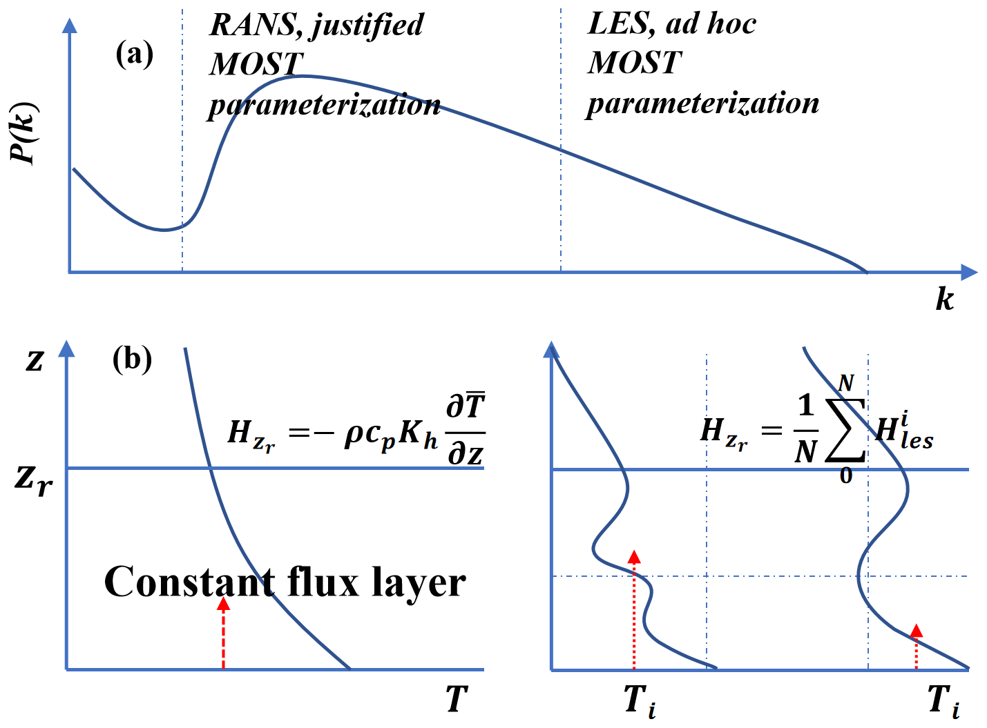
Figure 2 (a) Schematic energy spectrum of eddies, P(k), as a function of wave number k. (b) Schematic profile of T in Reynolds-averaged Navier–Stokes (RANS) models (left) and LES models (right). z_r is the height of the constant flux layer.

We use sensible heat flux for the discussion of the macroscopic constraint. A correction to $H_{\mathrm{les}}^i$ is made to ensure adherence to Eq. (15), namely,

$$\begin{array}{}\text{(16)}& H_{\mathrm{les},\mathrm{new}}^i=\mathit{\mu }{H}_{\mathrm{les}}^i,\end{array}$$

and

$$\begin{array}{}\text{(17)}& \mathit{\mu }={\displaystyle \frac{H_{\mathrm{most}}}{\frac{\mathrm{1}}{N}{\sum }_{i=\mathrm{1}}^{i=N}{H}_{\mathrm{les}}^i}},\end{array}$$

where $H_{\mathrm{les},\mathrm{new}}^i$ is the updated surface sensible heat flux. We apply the proposed MOST correction up to a height of 50 m. This correction indeed pertains to the constant flux layer. At the surface, vertical velocity $w_{\mathrm{g}}^i=\mathrm{0}$, and $H_{\mathrm{les}}^i$ is entirely subgrid, i.e.,

$$\begin{array}{}\text{(18)}& H_{\mathrm{les}}^i=-\mathit{\rho }{C}_{\mathrm{p}}{K}_{\mathrm{h},\mathrm{sg}}^i{\displaystyle \frac{\partial T_{\mathrm{g}}^i}{\partial z}},\end{array}$$

Hence, the macroscopic constraint becomes a constraint on the LES subgrid eddy diffusivity,

$$\begin{array}{}\text{(19)}& K_{\mathrm{h},\mathrm{sg},\mathrm{new}}^i=\mathit{\mu }{K}_{\mathrm{h},\mathrm{sg}}^i.\end{array}$$

The same formulation applies to latent heat flux and momentum flux.

In practice, H_most can be estimated as follows. Suppose the LES domain consists of J land use types, with σ_j being the fraction of land use type j. Then, H_most can be approximated using the mosaic approach (see Niu et al., 2011),

$$\begin{array}{}\text{(20)}& H_{\mathrm{most}}={\sum }_j{\mathit{\sigma }}_j{H}_j\end{array}$$

and

$$\begin{array}{}\text{(21)}& H_j=-{\mathit{\alpha }}_j\mathit{\rho }{C}_{\mathrm{p}}{\displaystyle \frac{\left({\stackrel{\mathrm{‾}}{T}}_{\mathrm{a},j}-{\stackrel{\mathrm{‾}}{T}}_{\mathrm{0},j}\right)}{{\stackrel{\mathrm{‾}}{r}}_{\mathrm{h},j}}},\end{array}$$

where ${\stackrel{\mathrm{‾}}{T}}_{\mathrm{a},j}$, ${\stackrel{\mathrm{‾}}{T}}_{\mathrm{0},j}$, and ${\stackrel{\mathrm{‾}}{r}}_{\mathrm{h},j}$ are mean air temperature, mean surface temperature, and aerodynamic resistance for land use type j from the LES domain, respectively. The parameter α_j represents the efficiency factor of H_most for land use type j. Further elucidation regarding the determination of the α values can be found in the Supplement.

3 Field observations and numerical experiments

3.1 Observation site and data

We employed the multi-scale evapotranspiration flux observation datasets over heterogeneous land surfaces in the Heihe River Basin from HiWATER (Liu et al., 2011; Li et al., 2013). These datasets encompass observations from various sites, including the Daman site (38.85^∘ N, 100.37^∘ E; 1556.00 m a.s.l.), Village site (38.85^∘ N, 100.35^∘ E; 1561.87 m a.s.l.), Orchard site (38.84^∘ N, 100.36^∘ E; 1559.63 m a.s.l.), and radiosonde sounding observations from the Zhangye National Climate Observatory (39.08^∘ N, 100.27^∘ E; 1556.06 m a.s.l.) (Fig. 3). The Daman, Village, and Orchard sites were situated in the agricultural fields of the Daman irrigation area in the city of Zhangye, China, featuring maize fields, villages, and orchards as representative land surfaces, respectively. Several sensors recorded meteorological data at varying heights above the ground. Specifically, wind speed and wind direction sensors were installed at heights of 3, 5, 10, 15, 20, 30, and 40 m. An air pressure sensor was placed at 2 m above the ground. Additionally, a four-component radiometer was mounted at 12 m. Soil temperature probes were deployed at the soil surface (0 cm) and depths of 2, 4, 10, 20, 40, 80, 120, and 160 cm, all located 2 m south of the meteorological tower. Soil moisture sensors were buried at depths of 2, 4, 10, 20, 40, 80, 120, and 160 cm, all positioned 2 m south of the meteorological tower.

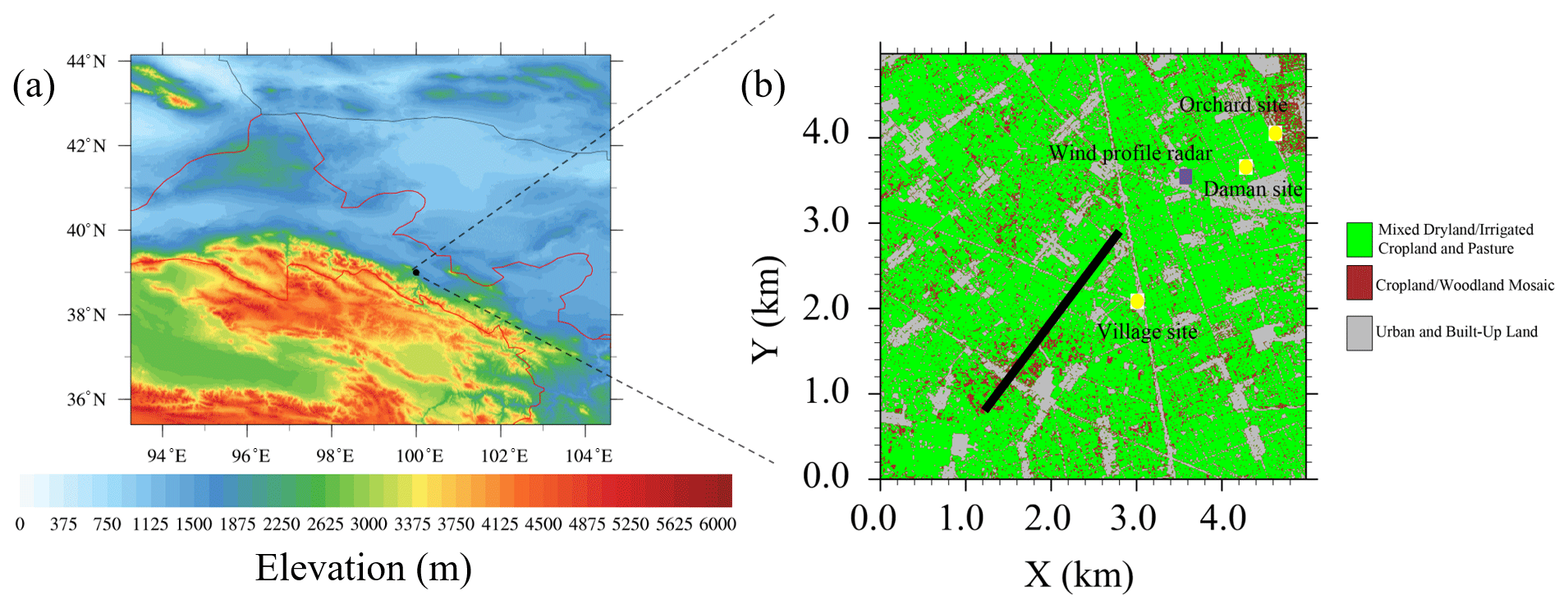
Figure 3 (a) The location of the observation site and (b) the land use map. In panel (b), the solid black line is the optical length of a large aperture scintillometer (LAS).

The eddy covariance (EC) systems at the Daman, Village, and Orchard sites were mounted at 4.5, 6.2, and 7.0 m, respectively, with all systems operating at a sampling frequency of 10 Hz. These systems were consistently oriented northward, and the distance between the sonic anemometer (CSAT3) and the ${\mathrm{CO}}_{\mathrm{2}}/{\mathrm{H}}_{\mathrm{2}}\mathrm{O}$ analyzer (Li7500A) was maintained at 17, 20, and 10 cm, respectively. The collected EC data underwent rigorous preprocessing to ensure data quality. The EC data were initially temporally aggregated into 30 min intervals to facilitate subsequent analysis. Furthermore, the quality of the observational data underwent a classification process that stratified data quality into distinct levels based on criteria such as Δst (stationarity) and integral turbulent characteristics (ITCs) using the methodology outlined by Foken and Wichura (1996). Only data within class 1, representing high-quality data (Δst <30 and ITC <30), were considered. A five-step data quality control process was also implemented for the half-hourly flux data. These steps involved eliminating data obtained during periods of sensor malfunction, characterized by anomalous diagnostic signals and automatic gain control values exceeding 65; rejecting data collected within 1 h of precipitation events; discarding incomplete 30 min data segments if missing data accounted for more than 3 % of the raw 30 min record; excluding data acquired during nighttime hours when the friction velocity (u_∗) fell below 0.1 m s⁻¹ (Blanken et al., 1998); and considering only wind directions ranging from 315 to 0 and 0 to 45^∘ to mitigate potential influences from adjacent EC sensors or environmental factors such as nearby brackets.

3.2 Real-case numerical experiment

The real-case experiments were conducted over a homogeneous surface which includes three distinct land use types: “mixed dryland–irrigated cropland and pasture” (hereafter MDICP) (representing the Daman site), “urban and built-up land” (hereafter UBL) (representing the Village site), and “cropland–woodland mosaic” (hereafter CWM) (representing the Orchard site) (Fig. 3b). The simulation domain was a 5 km × 5 km area, represented by 100 × 100 grid points, with a horizontal grid spacing of $\mathrm{\Delta }x=\mathrm{\Delta }y=\mathrm{50}$ m. Vertically, the domain extends to a height of 2.6 km, divided into 100 layers, with a resolution Δz stretching from 10 to 40 m. A Rayleigh damping layer was implemented at a height of 500 m from the top to damp the gravity waves. Initial profiles for horizontal wind speed, potential temperature, and humidity were extracted from the soundings conducted at the Zhangye station at 08:00 local time (LT) on 20 August 2012 (Fig. 4). Solar shortwave radiation and upward longwave radiation fluxes observed at the Daman site from 08:00 to 18:00 LT were used to force the model. Initial soil temperature and soil moisture conditions for MDICP, UBL, and CWM were derived from observations collected at 08:00 LT on 20 August 2012, at the Daman, Village, and Orchard sites, respectively. Each simulation spanned 10 h, during which the weather conditions were sunny and free from influences of weather systems. The choice of physics parameterization schemes was as follows: the 1.5-order TKE closure (Deardorff, 1980; Zhang et al., 2018) was selected for subgrid closure, while the revised MM5 Monin–Obukhov scheme (Jimenez and Dudhia, 2012) was employed for the surface layer. The roughness lengths z_0 s for different land use types were obtained from a lookup table (LANDUSE.TBL). For MDICP, CWM, and UBL, the α values of 0.94, 0.94, and 1.03 were assigned to the sensible heat flux, while for the latent heat flux, the values were 0.92, 0.92, and 1.09, respectively, based on the method in the Supplement.

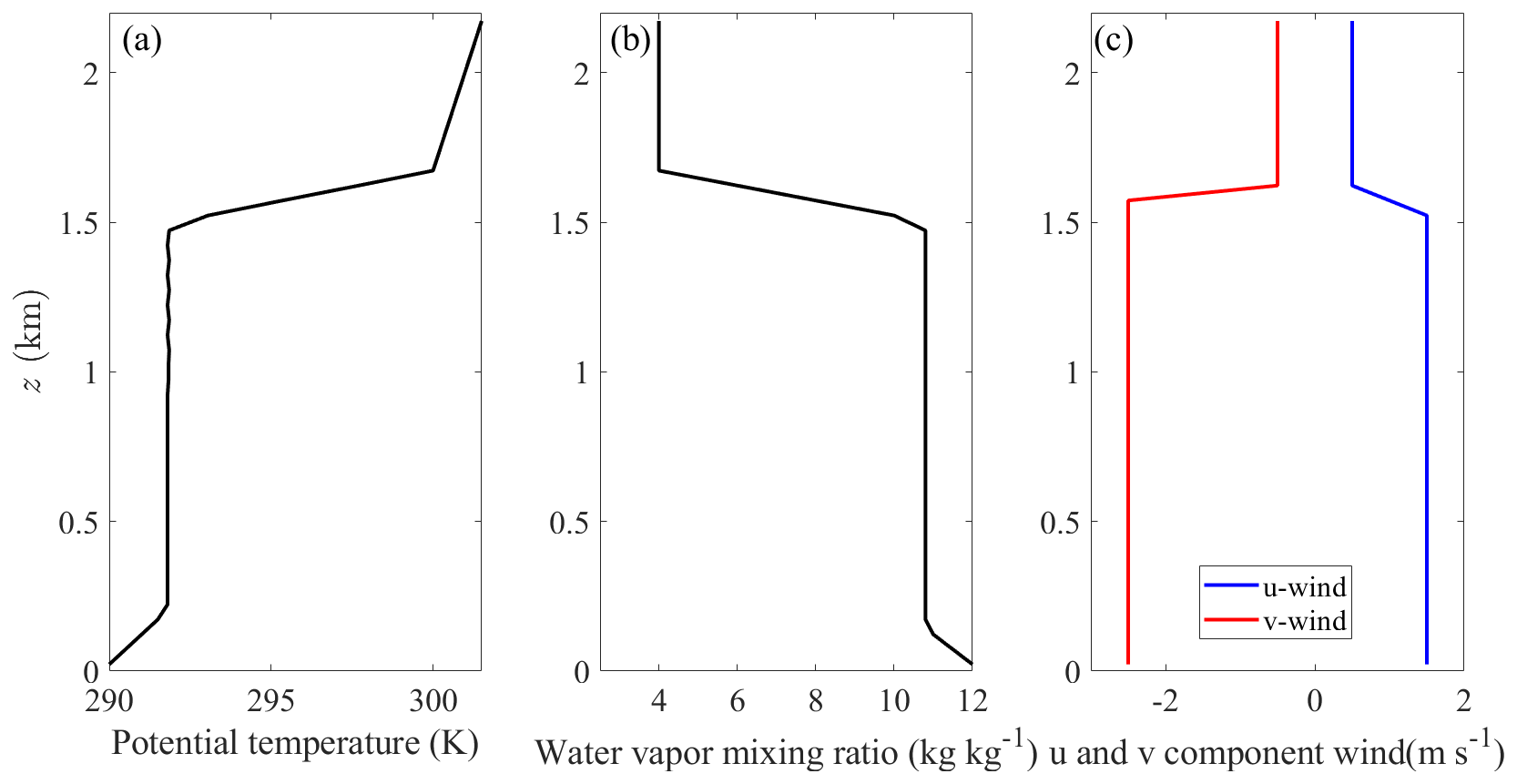
Figure 4 (a) Initial potential temperature, (b) water vapor mixing ratio, and (c) u and v components of wind speed, derived from the soundings at the Zhangye station (39.08^∘ N, 100.27^∘ E; 1556.06 m a.s.l.) at 08:00 LT on 20 August 2012.

We employed three distinct surface flux schemes for comparison. The new MOST-r scheme is evaluated alongside two other existing schemes: the Noah-MP land surface scheme, which incorporates MOST-based flux formulations coupled to LES (referred to as LES-Noah), and the local flux calculation scheme developed by Shao et al. (2013) (referred to as LES-S13). The observed sensible and latent heat fluxes, averaged from three EC sites, were used as the benchmark for evaluating the LES simulated sensible and latent heat fluxes using the three schemes. The simulated sensible and latent heat flux at a height of 10 m was juxtaposed with these observations for validation purposes.

Furthermore, the effects of varying horizontal grid resolutions on the MOST-r results were investigated by changing the model grid spacing Δx=Δy from 100 to 10 m. Concomitant adjustments were made to the time steps to maintain numerical stability. The details of the sensitivity experiments are listed in Table 1. The root mean square error (RMSE) was used to measure the difference between different methods and ground-measured data:

$$\begin{array}{}\text{(22)}& \text{RMSE}={\left[M^{-\mathrm{1}}{\sum }_{i=\mathrm{1}}^{i=M}{\left(f_{\mathrm{obs}}^i-f^i\right)}^{\mathrm{2}}\right]}^{\mathrm{1}/\mathrm{2}},\end{array}$$

where M is the number of observations, $f_{\mathrm{obs}}^i$ is the fluxes measured by EC system, and fⁱ is the fluxes calculated by different methods.

Table 1 Lists of sensitivity experiments.

4 Results

4.1 Correction of MOST-r

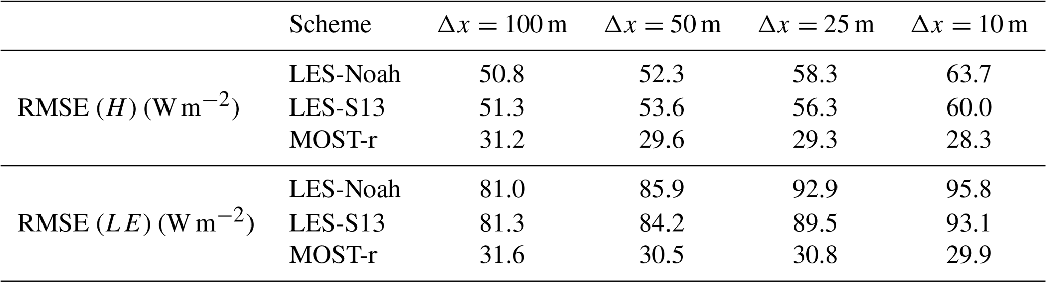
We have conducted a comparative analysis involving LES-Noah, LES-S13, and MOST-r. To evaluate the correction of MOST-r for H and LE quantitatively, RMSEs for time- and domain-averaged H and LE between different experiments and observations are calculated and shown in Table 2. The estimated H and LE computed by MOST-r are closer to the observations than those by LES-Noah and LES-S13 methods. For example, when Δx=5 m, MOST-r has corrections of 22.7 W m⁻² for H and 55.4 W m⁻² for LE compared with LES-Noah. Similarly, compared to LES-S13, MOST-r has corrections of 24.0 W m⁻² for H and 53.7 W m⁻² for LE, respectively. In general, MOST-r consistently outperforms the other two methods, with LES-S13 yielding the second-best results, while LES-Noah displays the least favorable outcomes.

Table 2 RMSE between different experiments and observations for time- and domain-averaged H and LE.

4.2 Profiles of the time- and domain-averaged fluxes estimated by MOST-r

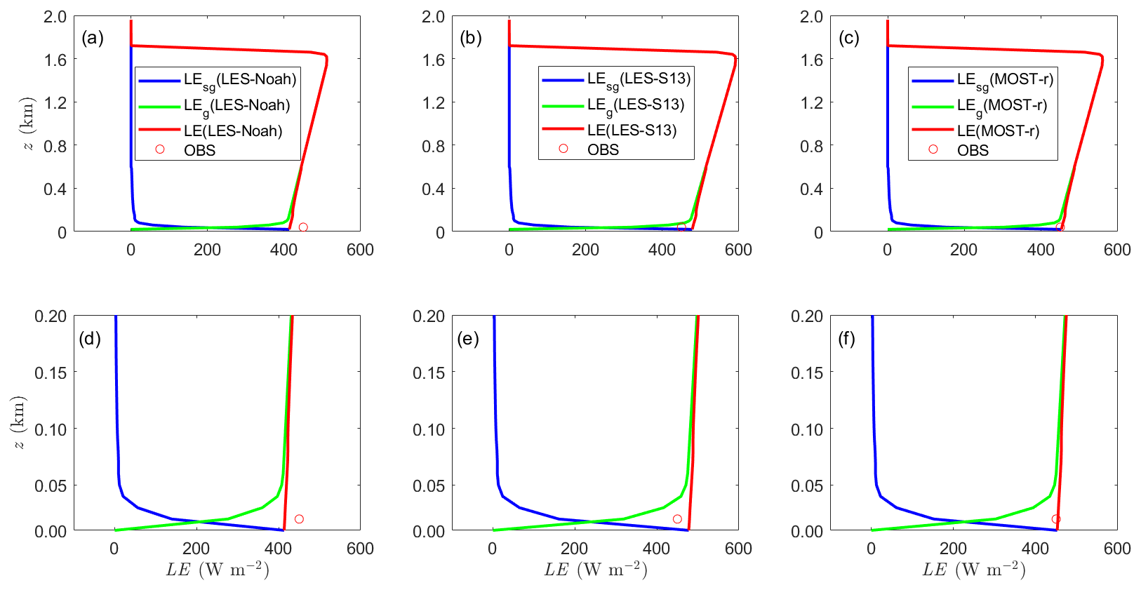
Profiles of the time- and domain-averaged sensible heat fluxes (H, H_g, and H_sg) and latent heat fluxes (LE, LE_g and LE_sg), as estimated by LES-Noah, LES-S13, and MOST-r, and observations, are shown in Figs. 5–6. H estimates derived from MOST-r are generally closer to the measurements than those by LES-Noah and LES-S13 (Fig. 5a–c). Profiles of H estimated by LES-Noah, LES-S13, and MOST-r decrease with height linearly near the surface, extending until the inversion layer (Fig. 5d–f). This behavior is similar to the findings in Shao et al. (2013). In the bulk of the boundary layer, H is primarily attributed to H_g, with H_sg playing a negligible role. Close to the surface, H_sg takes precedence when turbulence occurs at finer scales. Similarly, LE estimates yielded by MOST-r are generally closer to the measurements than those by LES-Noah and LES-S13 (Fig. 6d–f). The near-surface flux estimated by MOST-r varies little with height, effectively meeting the assumptions associated with a constant flux layer. Our earlier analysis in Sect. 2.2 and reference to Eq. (15) reveal that the flux within the constant flux layer differs between RANS and LES. Traditional LES-Noah failed to align with MOST, resulting in fluctuations in the constant flux layer as a function of height. LES-S13, devoid of MOST constraints, yields inferior results. In this regard, MOST-r represents a significant improvement, with H_sg estimates generated by MOST-r surpassing those derived from LES-S13.

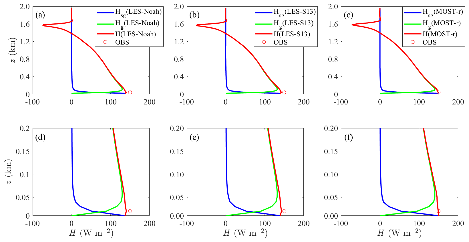
Figure 5 Profiles of H (red line), H_g(green line), and H_sg (blue line) estimated by (a) LES-Noah, (b) LES-S13, and (c) MOST-r averaged over the model domain and during 12:00–13:00 LT. Profiles of H (red line), H_g (green line), and H_sg (blue line) estimated by (d) LES-Noah, (e) LES-S13, and (f) MOST-r for the lower 200 m. The red circle is the averaged observation from three EC systems. The horizontal grid spacing is set to Δx=50 m for the large-eddy simulations.

Figure 6 Same as Fig. 5 but for latent heat flux.

4.3 Patterns of surface H and LE estimated by MOST-r

The study compares surface sensible heat (H) and latent heat (LE) flux patterns estimated by LES-Noah, LES-S13, and MOST-r. All patterns were temporally averaged between 12:00 and 13:00 LT (Fig. 7a–f). The patterns of H and LE estimated by MOST-r exhibit a striking similarity with those by LES-Noah and LES-S13. This parallelism indicates that MOST-r's constraining influence over heterogeneous surface conditions effectively maintains the overall pattern of heat flux. This phenomenon is intriguing and signifies the adaptability of MOST-r's constraints in accommodating varying surface characteristics without fundamentally altering the heat flux pattern. Furthermore, the patterns of H and LE by MOST-r demonstrate a concordance with the patterns of land use. For example, the UBL regions exhibit the highest H (>300 W m⁻²) estimated by MOST-r. Conversely, the H estimated by MOST-r over the MDICP and CWM is lower, hovering around 100 W m⁻². The maximum LE (>500 W m⁻²) is concentrated over the MDICP areas, whereas the LE over the UBL is much lower, at around 200 W m⁻². In short, the H and LE patterns closely mirror the distinctive characteristics of the underlying land use.

The bilinear interpolation of grid point results from within the LES domain to approximate values at specific observation points was used to allow for a direct comparison between estimations and observations. In particular, the focus is on areas classified as MDICP and UBL. Over the MDICP and UBL, the estimated H and LE computed by MOST-r are closer to the EC observations than those by LES-Noah and LES-S13 methods (Fig. 8). The investigation extends to several other critical parameters, namely net radiation flux (R_net), surface skin temperature (T_s), and ground heat flux (G), where the estimations in real-case scenarios are cross-referenced with measurements (Fig. 9). Over MDICP and UBL, the estimated R_net values by MOST-r are closer to the observations than those by LES-Noah and LES-S13. For example, the simulated R_net by MOST-r is up to 50 W m⁻² higher than the observed values. In contrast, R_net by LES-S13 is more than 100 W m⁻² higher than the observed values. Furthermore, the R_net over UBL by all methods is smaller than that over MDICP. The assessment extends to surface skin temperature (T_s), revealing that MOST-r achieves a notably superior agreement with observations over MDICP and UBL. In contrast, LES-Noah and LES-S13 tend to overestimate T_s by up to 3 ^∘C compared to observed values. Consistent with the R_net findings, T_s is generally higher over UBL than MDICP across all methods. The G estimated by MOST-r matches the observations and is better than that by LES-Noah and LES-S13 over MDICP and UBL. In contrast, LES-Noah tends to overestimate G by up to 30 W m⁻² over MDICP, further underscoring the proficiency of MOST-r. These findings affirm that MOST-r consistently outperforms LES-Noah and LES-S13 in providing estimations that closely align with observations across a spectrum of critical parameters.

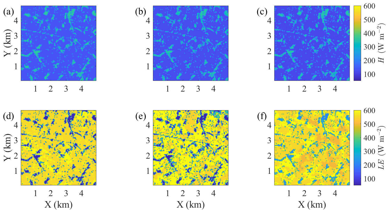
Figure 7 Patterns of surface sensible heat flux (H) estimated by (a) LES-Noah, (b) LES-S13, and (c) MOST-r averaged during 12:00–13:00 LT. Panels (d), (e), and (f), as panels (a), (b), and (c), respectively, but for latent heat flux (LE). The horizontal grid spacing is set to Δx=50 m for the large-eddy simulations.

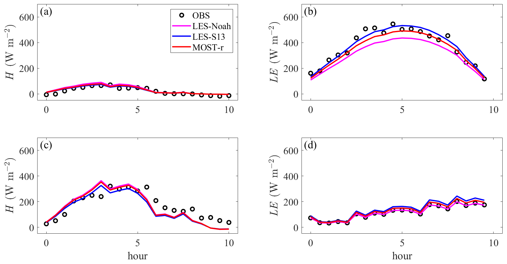
Figure 8 Time series of (a) sensible heat flux H and (b) latent heat flux LE, for the MDICP surface, from observations and LES simulations using the LES-Noah, LES-S13, and MOST-r method with Δx=50 m. Panels (c) and (d) are as panels (a) and (b), respectively, but for the UBL surface.

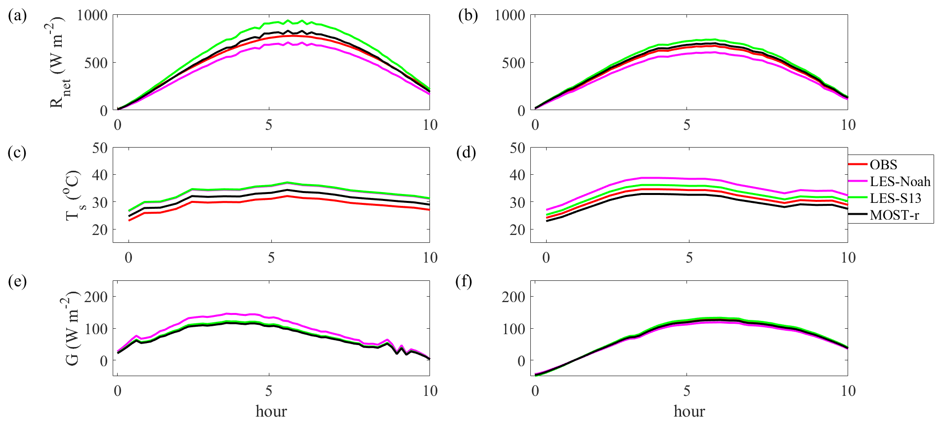
Figure 9 (a) Net radiation flux (R_net), (c) surface temperature (T_s), and (e) ground heat flux (G) from observations and estimated using the LES-Noah, LES-S13, and MOST-r methods over MDICP. Panels (b), (d), and (f) are as panels (a), (c), and (e), respectively, but for the UBL surface.

4.4 The effect of horizontal grid spacing on the correction by MOST-r

To better understand the impact of horizontal grid spacing (Δx) on the corrective capacity of MOST-r, a series of sensitivity experiments were conducted by varying the horizontal grid spacing. The findings of these experiments are shown in Fig. 10 and Table 2. The corrective influence exerted by MOST-r on H and LE remains remarkably consistent as the horizontal grid spacing is progressively reduced (Fig. 10a–b). In contrast, surface H_les and LE_les estimated by LES-S13 decrease as Δx decreases, indicating that Δx has a large effect on surface H_les and LE_les estimated using LES-S13. These results are similar to those in Shin and Hong (2013), where the domain-averaged subgrid fluxes decrease with the decrease in Δx, while the resolved fluxes increase. We see from these experiments that the MOST-r scheme maintains its corrective efficacy across varying horizontal grid spacings without exhibiting undue sensitivity to this parameter.

To reveal the impact of horizontal grid spacing (Δx) on the macroscopic constraint imposed by MOST, we present an analysis of the μ parameter. As shown in Fig. 10c, the value of μ increases as Δx decreases. Specifically, μ for H increases from 1.00 for Δx=100 m to 1.68 for Δx=25 m. In addition, μ for LE is smaller than that for H, indicating that the macroscopic constraint imposed by MOST on H is larger than that on LE (Fig. 10c).

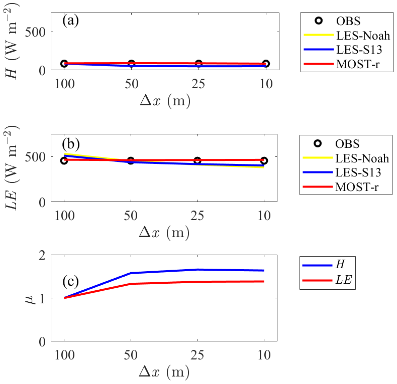
Figure 10 (a) H and (b) LE by observation, LES-Noah, LES-S13, and MOST-r averaged over the model domain and during 12:00–13:00 LT with different horizontal grid spacing (Δx= 100, 50, 25, 10 m). Variations of (c) μ for H and LE with different horizontal grid spacing (Δx= 100, 50, 25, 10 m) averaged over the model domain and during 12:00–13:00 LT.

5 Conclusion and discussion

In response to the inconsistencies in using MOST for parameterization of surface fluxes in LES models and the deficits of the scheme proposed by Shao et al. (2013), we presented here the MOST-r scheme suitable for flux estimates of LES models. MOST-r consists of two components: first, it computes LES subgrid fluxes using eddy viscosity and diffusivity estimates from the LES closure tailored to local turbulence characteristics, and second, it incorporates a macroscopic constraint, which aligns fluxes averaged over the LES domain with MOST principles.

We conducted a series of real-case experiments over an oasis surface in northwestern China, employing the MOST-r scheme. Comparative analyses were performed, putting the Noah-MP coupled with LES (LES-Noah) and the LSM in Shao et al. (2013) coupled with LES (LES-S13) against the new scheme. MOST-r consistently outperforms the other two schemes, with LES-S13 yielding the second-best results, while LES-Noah showed somewhat less favorable outcomes. Traditional LES-Noah failed to adhere to the MOST principles, causing flux discrepancies within the constant flux layer as a function of height. On the other hand, LES-S13, lacking the MOST constraints, provided less accurate outcomes than the MOST-r scheme. MOST-r thus stands as a substantial improvement, with its ability to adhere to MOST on large scales, particularly regarding the sensible heat flux estimates. It is noted that the MOST-r scheme's constraining effect preserves the spatial patterns of the fluxes. This feature of the MOST-r scheme enables the LES model to correctly reproduce the spatially averaged fluxes while maintaining the flux patterns arising from surface heterogeneity. Our tests consistently demonstrate MOST-r's superiority over LES-Noah and LES-S13, aligning more closely with the observations of various key surface variables. Sensitivity experiments regarding horizontal resolution reveal that the MOST-r scheme produces grid-resolution invariant fluxes and thereby remedies the major deficit of the schemes directly based on the MOST, such as the LES-Noah scheme. We observed that the macroscopic constraint imposed by MOST on LES strengthens as the horizontal grid spacing decreases, with a greater influence on H than on LE.

As previously mentioned, the two-part eddy viscosity model proposed by Sullivan et al. (1994) provided important insight into achieving alignment of subgrid closure with MOST across different spatial scales. But as far as flux estimates in LES models are concerned, the use of eddy viscosity and diffusivity derived from the LES turbulent closure accounts for the heterogeneities on scales larger than the LES model resolution. Hence, the MOST-r scheme already integrated the basic ideas of the two-part eddy viscosity model of Sullivan et al. (1994), without invoking the assumption of reduced turbulent contribution to subgrid eddy viscosity and diffusivity. This enables the MOST-r scheme to better model the surface flux patterns. Instead of attempting to derive a general scale-invariant scheme for flux estimates, we provided a scheme that is both simple and effective for LES models.