Water vapour exchange between the atmospheric boundary layer and free troposphere over eastern China: seasonal characteristics and the El Niño–Southern Oscillation anomaly

This study develops a quantitative climatology of water vapour exchange between the atmospheric boundary layer (ABL) and free troposphere (FT) over eastern China. The exchange flux is estimated for January, April, July and October over 7 years based on a water vapour budget equation using simulated meteorological data. The spatiotemporal characteristics and occurrence mechanism of ABL–FT water vapour exchange and its relationship with the El Niño–Southern Oscillation (ENSO) are revealed: (1) the vertical exchange flux varies regionally and seasonally, with downward transport to maintain ABL moisture during winter and autumn in the northern region and persistent output to humidify the FT in the southern region, particularly in summer. Additionally, the vertical exchange flux is also topographic dependent. (2) The vertical motion at the ABL top, which is produced by the dynamic forcing of the terrain on synoptic winds, is the dominant mechanism for the water vapour vertical exchange over the long-term average. The evolution of the vertical exchange flux within 1 d scale is driven by the ABL diurnal cycle. (3) The interannual variation of water vapour vertical exchange is correlated with ENSO. A triple antiphase distribution with negative–positive–negative anomalies from north to south exists in La Niña years (and vice versa in El Niño years), which corresponds to the spatial pattern of anomalous precipitation. This phenomenon is mainly due to the alteration of vertical velocity and water vapour content at the ABL top varying with ENSO phases. These results provide new insight into understanding the atmospheric water cycle.

1 Introduction

Water vapour is a significant constituent in the atmosphere. It directly participates in fundamental physical processes, including cloud formation, precipitation, severe weather development and atmospheric circulation (Sodemann and Stohl, 2013; Wong et al., 2018; Wypych et al., 2018). Water vapour also affects important chemical reactions, such as providing OH radicals for gaseous photochemical transformations and serving as a medium in secondary aerosol formations (Pilinis et al., 1989; Tabazadeh 2000; Wu et al., 2019). Moreover, the radiation forcing of water vapour accounts for about two-thirds of the total natural greenhouse effect, which plays a vital role in climate feedback (Kiehl and Trenberth, 1997; Harries et al., 2008; Adebiyi et al., 2015).

The distribution of water vapour in the atmospheric system depends on its source and transport processes. In general, water vapour evaporates from the Earth's surface into the atmosphere. From the meridional and zonal view, it presents a transport trend from low latitude to high latitude and from ocean to land. The horizontal transport of water vapour has been widely discussed from multiple scales. Hemispheric-scale atmospheric rivers induce large excursions of high vertically integrated water vapour from the subtropics to high latitudes (Newell et al., 1992; Zhu and Newell, 1998; Sodemann and Stohl, 2013). Synoptic-scale moisture flux convergence of extratropical cyclones explains the precipitations and cloud structures over the warm front and cold front (Boutle et al., 2010; Wong et al., 2018). Regional-scale transport processes are widely reported in many areas from water vapour advection and dynamical convergence (Zhou and Yu, 2005; Sun et al., 2010; Gvozdikova and Muller, 2021). However, these studies estimate vertically integrated water vapour through the atmospheric layer (usually from the surface to 300 hPa) or only focused on a certain altitude.

Water vapour vertical transport, especially within the troposphere, plays a key role in the atmospheric water cycle. All water vapour in the atmosphere originates from surface evaporation and is first confined in the atmospheric boundary layer (ABL; Boutle et al., 2010), which is defined as the lowest layer of the atmosphere influenced by the Earth's surface (Stull, 1988). The water vapour is turbulently mixed in the ABL, making it act as a reservoir. Actually, all water vapour entering and transporting meridionally and zonally in the free troposphere (FT) is initially exported through the ABL (Bailey et al., 2013). In other words, the water vapour exchange between the ABL and the FT is a prerequisite for its large-scale transport and redistribution, as well as interaction with other constituents, in the upper atmosphere. Several studies indicate the importance of this key process in precipitation (Liu et al., 2020), cloud systems (Miura et al., 2007), tropical cyclone formation (Fritz and Wang, 2013), the Madden–Julian oscillation (Hirota et al., 2018), the West African monsoon jump (Hagos and Cook, 2007) and O₃ vertical distributions (Andrey et al., 2014). Therefore, it is of great significance to quantify the vertical exchange of water vapour between the ABL and FT.

However, the exchange between the ABL and FT is not straightforward, both for water vapour and air mass. Although the diurnal variation of the ABL depth allows air constituents to be entrained into and left out of this layer within its variation range, the actual exchange between ABL and FT is small on the timescale of more than 1 d due to the cancelling effect (Hov and Flatoy, 1997; Jin et al., 2021). The current studies on water vapour vertical transport are mainly limited to complex terrain areas or special convective events. The local/mesoscale circulation induced by orographic thermal and dynamic effects is considered a key process for ABL ventilation (Kossmann et al., 1999; McKendry and Lundgren, 2000; Dacre et al., 2007). Henne et al. (2005) found that there were elevated moisture layers in the lower free troposphere in the lee of the Alps resulting from mountain venting. On average for the 12-year period, ∼ 30 % of the water vapour of the Alpine boundary layer was vented to the FT per hour during the daytime, which makes the total precipitable water within the elevated moisture layer increase by ∼ 1.3 mm. Another simulated study indicates that the moisture exchange between the ABL and FT of mountainous topography can be about 3–4 times larger than the amount of moisture evaporated from the surface in a specific ventilation event (Weigel et al., 2007). The convective system, mainly mesoscale deep and shallow convection, is another important factor leading to the vertical transport of water vapour. The isotope observations show that the moisture transport pathways to the subtropical North Atlantic FT are linked to dry convection processes over the African continent which effectively inject humidity from the ABL to higher altitudes (Gonzalez et al., 2016; Dahinden et al., 2021). The water vapour budget of the free troposphere of the maritime tropics shows that 20 % of this source comes from vertical convective transport (Sherwood, 1996). On the other hand, an idealized simulation suggests that the warm conveyor belt ascent and shallow convective processes contributed about equally to FT moisture (Boutle et al., 2010, 2011).

Despite these studies, general characteristics of long-term and wide-ranging ABL–FT water vapour exchange are still unknown. These characteristics are closely bound up with the atmospheric energy flow and the entire climate system, affecting clouds, precipitation and radiation (Sodemann and Stohl, 2013; Wong et al., 2018; Wypych et al., 2018). For example, small variations in upper atmospheric humidity over a large spatial–temporal scale can cause systemic changes in the hydrological cycle and atmospheric circulation (Minschwaner and Dessler, 2004; Sherwood et al., 2010; Allan, 2012). The climate state of water vapour vertical exchange flux is critical for quantifying these specific effects. To fill this knowledge gap, the present study calculates the water vapour exchange flux between the ABL and FT for 7 years (2011 and 2014–2019) over eastern China (20–42^∘ N, 108–122^∘ E) to establish the first quantitative climatology view on this issue. The water vapour budget method is used, with the mesoscale meteorological simulation providing input data. January, April, July and October, respectively representing winter, spring, summer and autumn, are considered to discuss the seasonal characteristics. Interannual differences are analysed by investigating the impact of El Niño and La Ninã events. On the basis of understanding the foundational features, we further attempt to discuss the role that ABL–FT water vapour exchange plays in anomalous precipitation. The arrangement of this paper is as follows. Data and methods are described in Sect. 2. The seasonal characteristics and mechanism analysis, interannual variability, and the relation with anomalous precipitation are presented and discussed in Sect. 3. Finally, the findings of this study are summarized in Sect. 4.

2 Data and methods

2.1 Observation data

Intensive ABL sounding data and routine surface meteorological data were used to evaluate the performance of the Weather Research Forecast (WRF) model that provided the input data for estimating exchange flux.

Intensive ABL sounding data. Two field experiments of intensive GPS (Global Positioning System) sounding were carried out in Dezhou (37^∘16^′ N, 116^∘43^′ E), located in the middle of the North China Plain (NCP) (Fig. 1b), from 25 December 2017 to 24 January 2018 and from 14 May to 14 June 2018. Eight soundings were taken for each day, at 02:00, 05:00, 08:00, 11:00, 14:00, 17:00, 20:00 and 23:00 LT (i.e., UTC + 8). A GPS radiosonde (Beijing Changzhi Sci and Tech Co. Ltd., China) was used to obtain profiles of wind, temperature and humidity, with the ascending velocity being about 3–5 m s⁻¹. We eliminated the outliers from the original data and averaged the profiles to an effective vertical resolution of 10 m. ABL heights were determined with these data via the potential temperature profile method (Liu and Liang, 2010). The reliability of the GPS sounding data has been systematically evaluated by Li et al. (2020) and Jin et al. (2020).

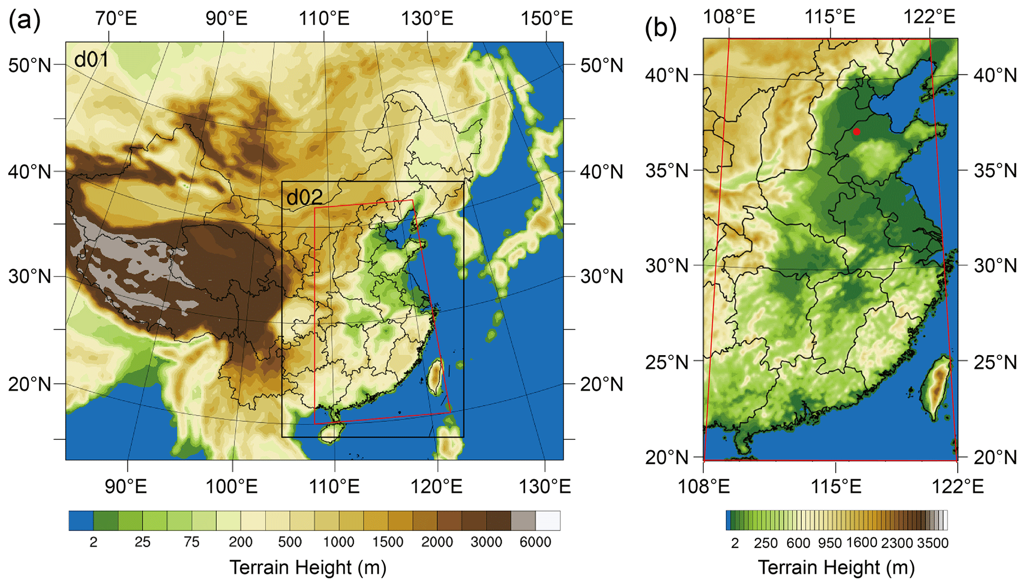
Figure 1 Geographical map of (a) the Weather Research and Forecast (WRF) model domains (d01 and d02) and (b) the amplified research domain (marked with red lines). The map uses the Lambert projection with the centre meridians of 108^∘ E in (a) and 115^∘ E in (b). The red dot in (b) indicates the intensive GPS sounding observatory. Publisher’s remark: please note that the above figure contains a disputed territory.

Routine surface meteorological data. The hourly surface data of 137 routine observatories distributed within the research domain were collected from the Chinese National Meteorological Center. The dataset included information on wind speed and direction, air temperature, relative humidity, air pressure, cloud coverage, and precipitation, which was used to evaluate the WRF simulation.

2.2 Three-dimensional meteorological simulation

The WRF model was conducted to provide three-dimensional meteorological data for the estimation of ABL–FT water vapour exchange flux. Two nested domains (Fig. 1a) were employed with horizontal grid lengths of 30 and 10 km, respectively. The inner domain covered eastern China (20–42^∘ N, 108–122^∘ E), the main research region for the ABL–FT water vapour exchange in the present work (Fig. 1b). Each domain had 37 vertical layers extending from the surface to 100 hPa, with the vertical resolution being about 20–30 m below 200 m, increasing to ∼ 100 m at 750 m, ∼ 250 m at 2000 m, ∼ 350 m at 3000 m, ∼ 600 m at 5000 m, ∼ 900 m at 8000 m and ∼ 1300 m at 11000 m and gradually enlarging to the top of the model. There were 24 layers within 3 km to resolve the ABL and its upper FT. The meteorological initial and boundary conditions were set using the US National Center for Environmental Prediction Final Analysis (NCEP-FNL) dataset.

In order to adequately reproduce water vapour distribution and to correctly estimate the ABL–FT exchange flux, sensitivity simulations were carried out to choose reasonable physical parameterization schemes. We focused on the microphysical and cumulus parameterizations that are the most relevant to the moisture simulation. Microphysics in the model includes explicitly resolved water vapour, cloud and precipitation processes. Cumulus schemes are responsible for the sub-grid-scale effects of convection and/or shallow clouds. Vertical fluxes due to unresolved updrafts and downdrafts are represented. The Lin et al. scheme (Lin et al., 1983) and WRF Single-Moment 6-class (WSM6) scheme (Hong and Lim, 2006) in microphysics parameterization, and the Grell–Devenyi (GD) ensemble scheme (Grell and Devenyi, 2002) and Kain–Fritsch (KF) scheme (Kain, 2004) in cumulus parameterization were compared, which were most commonly used in previous moisture simulation studies (Perez et al., 2010; Gonzalez et al., 2013; Jain and Kar, 2017; Qian et al., 2020). Other physics parameterization schemes used in this study included the Yonsei University PBL (planetary boundary layer) scheme (Hong et al., 2006), the Noah land surface model (Chen and Dudhia, 2001), the Dudhia short-wave radiation scheme (Dudhia, 1989) and the rapid radiative transfer model (Mlawer et al., 1997) for long-wave radiation. WRF simulations were initialized at 00:00 UTC on the day, and there was a 12 h spin-up time before the start of each 48 h simulation. Domain outputs were sampled every hour for the whole simulation period (January, April, July and October in 2011 and 2014–2019).

These schemes were evaluated by comparing simulated and observed specific humidity, temperature and wind speed, from their near-surface temporal evolution and vertical spatial structure. Another two key parameters, ABL height and precipitation, were also investigated: the former directly affects the exchange flux results, and the latter characterizes the moisture budget. The hourly averages of model outputs were extracted from the grid points nearest to the observed sites for comparison. In the vertical direction, the modelled and sounding data were simultaneously interpolated into the same height with 10 m intervals ranging from 50 m to 3 km. Note that the ABL height was diagnosed with the potential temperature profile method both for the simulations and for observation data, rather than using the default bulk Richardson number method in the Yonsei University (YSU) scheme.

The results of sensitivity experiments showed that there were no appreciable differences among various microphysical and cumulus parameterization schemes (Tables S1 and S2). In comparison, the combination of the WSM6 scheme and GD scheme performed better in humidity simulation and was more effective in reproducing temperature, wind speed and ABL height, especially in summer (Table S2). Therefore, these schemes were used in the present study. Its simulation performance determines the reliability of the calculated flux results and thus a comprehensive evaluation is provided here. The spatial–temporal evolutions of modelled and observed meteorological fields are presented by the height–time cross sections of specific humidity, potential temperature and wind speed, as well as the ABL height and precipitation (Fig. 2). During the winter and summer months of the intensive GPS sounding, the simulated atmospheric thermal and dynamic structures were comparable with observations. The alternating between dry and wet atmospheric states (Fig. 2a–b), formation and decay of upper temperature inversion (Fig. 2c–d), and vertical location and temporal transition of the strong and weak wind layers (Fig. 2e–f) were successfully reproduced. Accordingly, a good correlation between the simulated and observed ABL height was achieved, both in terms of diurnal variation and synoptic evolution, lasting several days (Fig. 2g–h). The correlation coefficients were 0.71 and 0.84 during wintertime and summertime, respectively. It should be mentioned that there was a slight discrepancy in the modelled ABL heights (mean biases are about −70 and 120 m in winter and summer), which may further affect the identification of other parameters (such as the wind component) at the ABL top and lead to uncertainty in the calculation results. This impact will be quantitatively analysed in the “Results and discussion” section. Another concerned meteorological factor, the daily cumulative precipitation was also evaluated, which showed a consistent evolution in observation and simulation (Fig. 2i–j), with correlation coefficients as high as 0.99 and 0.91 (p<0.05) in winter and summer, respectively, demonstrating that the moisture budget is accurately captured by the WRF simulations. Overall, the model showed the ability to capture the major variation of observed atmospheric thermal–dynamical structures reasonably, which ensures the validity of the meteorological inputs for the ABL–FT exchange flux calculation.

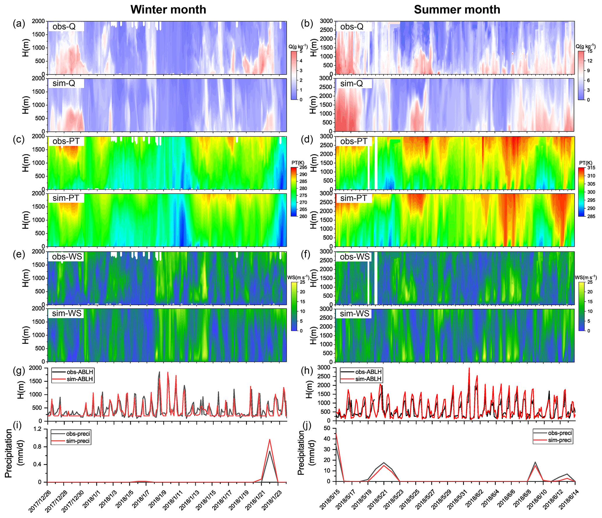
Figure 2 Observed and simulated time–height cross-sections of (a–b) specific humidity, (c–d) potential temperature, (e–f) wind speed, and temporal evolution of (g, h) ABL height and (i–j) daily cumulative precipitation at the Dezhou site (37.27^∘ N, 116.72^∘ E) during winter (from 26 December 2017 to 24 January 2018) and summer (from 15 May to 14 June 2018) months of the intensive GPS sounding field experiment. The time resolution of sounding data in (a, h) is 3 h. The y axis scales are different in the winter panels and the summer panels.

2.3 ABL–FT water vapour exchange flux

Similar to mass vertical exchange (Sinclair et al., 2010; Jin et al., 2021), the estimation of ABL–FT water vapour exchange flux in this study was based on an ABL water vapour budget equation established by Boutle et al. (2010):

$$\begin{array}{}\text{(1)}& \begin{array}{rl}{\displaystyle \frac{\partial }{\partial t}}\left({\int }_{\mathrm{0}}^h\mathit{\rho }q\mathrm{d}z\right)& =-\left({\displaystyle \frac{\partial }{\partial x}}{\int }_{\mathrm{0}}^h\mathit{\rho }qu\mathrm{d}z+{\displaystyle \frac{\partial }{\partial y}}{\int }_{\mathrm{0}}^h\mathit{\rho }qv\mathrm{d}z\right)\\ & +{\left(\mathit{\rho }q\right)}_h\left({\displaystyle \frac{\partial h}{\partial t}}\right)-{\left(\mathit{\rho }q\right)}_h{\left(\mathit{U}\cdot \mathit{n}\right)}_h-{\left(\mathit{\rho }\stackrel{\mathrm{‾}}{w^{\prime }{q}^{\prime }}\right)}_h\\ & +{\left(\mathit{\rho }\stackrel{\mathrm{‾}}{w^{\prime }{q}^{\prime }}\right)}_{\mathrm{0}}+P,\end{array}\end{array}$$

where ρ is air density; q is water vapour mixing ratio; h is ABL height; $\mathit{U}=(u,v,w)$ is wind vector; $\mathit{n}=(-\frac{\partial h}{\partial x},-\frac{\partial h}{\partial y},\mathrm{1})$ is the unit normal vector perpendicular to the ABL top surface; and w^′ and q^′ are the fluctuation values of vertical velocity and water vapour content, respectively. P is the precipitation. Subscripts h and 0 indicate quantities at the ABL top and the surface. The first term on the right side of Eq. (1) represents horizontal convergence/divergence within the ABL, the second term indicates the local change in ABL depth, the third term indicates vertical advection across the ABL top, the fourth and fifth terms are turbulent transport at the ABL top and the surface, respectively, and the last term indicates the net precipitation falling through the ABL.

Denoting the water vapour vertical exchange flux between the ABL and FT as F (positive values represent upward transport), it can be further written as

$$\begin{array}{}\text{(2)}& \begin{array}{rl}F& =-\left({\left(\mathit{\rho }q\right)}_h\left({\displaystyle \frac{\partial h}{\partial t}}\right)-{\left(\mathit{\rho }q\right)}_h{\left(\mathit{U}\cdot \mathit{n}\right)}_h-{\left(\mathit{\rho }\stackrel{\mathrm{‾}}{w^{\prime }{q}^{\prime }}\right)}_h\right)\\ & \approx -\left({\left(\mathit{\rho }q\right)}_h{\displaystyle \frac{\partial h}{\partial t}}+{\left(\mathit{\rho }q\right)}_h\left(u_h{\displaystyle \frac{\partial h}{\partial x}}+v_h{\displaystyle \frac{\partial h}{\partial y}}\right)-{\left(\mathit{\rho }q\right)}_h{w}_h\right).\end{array}\end{array}$$

Since turbulent transport between the ABL and FT is typically related with drier air that does not affect the total moisture content, ${\left(\stackrel{\mathrm{‾}}{w^{\prime }{q}^{\prime }}\right)}_h$ is usually considered to be a negligible contribution to the ABL–FT water vapour exchange flux (Boutle et al., 2010). Specifically, the finite difference method was adopted for calculation, with the time step being 1 h and the horizontal dimensions of the model grid being 10 km. The ABL heights were obtained from the hourly output of the WRF model. Other variables at the ABL top were extracted from the nearest model level above the ABL height (there is no significant difference between these extracted values and those interpolated to the ABL top). It is clear that the water vapour vertical exchange flux between the ABL and FT is determined by (i) the local temporal variation of ABL height, $\frac{\partial h}{\partial t}$, allowing the water vapour entrained into the ABL or left in the upper atmosphere; (ii) the spatial variation of the ABL, making water vapour horizontally advected across an inclined ABL top; and (iii) the vertical advection motion, carrying water vapour downward/upward through the interface between the ABL and FT. These three flux components are denoted as F_local, F_hadv and F_vadv, and their contributions and evolutions will be discussed in the following.

3 Results and discussion

The present study is based on a 7-year flux calculation. The years 2011 and 2014–2019 are selected for analysis, which includes typical La Niña, El Niño and neutral years (Marchukova et al., 2020; You et al., 2021; Felix Correia Filho et al., 2021), and are considered to be valid and concise datasets to reflect the characteristics of water vapour exchange between the ABL and FT. Their climatic representativeness is demonstrated using a long-term historical dataset provided by the fifth-generation ECMWF (European Centre for Medium Range Weather Forecasts) reanalysis (Hersbach et al., 2023, https://cds.climate.copernicus.eu/cdsapp#!/dataset/reanalysis-era5-pressure-levels?tab=form, last access: 20 October 2023). We compare the features of key meteorological elements during the study period (2011 and 2014–2019) and over the past 30 years (1990–2019) using the Kolmogorov–Smirnov test (K–S test) and histogram analysis. Temperature, the three-dimensional wind component, specific humidity both near the surface and at the upper level, and the ABL height and precipitation are studied. The K–S test indicates that there is no significant difference (with a confidence level of 95 %) between the 7-year sample period and the 30-year historical dataset for these variables (Table S3). The histogram analysis further illustrates that their normalized frequencies in the research samples are similar to those in the long-term historical data (Fig. S1). Also, the annual variation of the two sets of data presents a high consistency, with similar mean values and standard deviations (Fig. S2). The above analysis verifies that the 7-year samples adopted in this study can represent the long-term climatology and be promising to obtain climatic features of water vapour exchange between the ABL and FT. The basic temporal and spatial patterns, influencing mechanism, and relationship with the El Niño–Southern Oscillation (ENSO) and extreme precipitation are revealed as follows.

3.1 Seasonal generality and variability

3.1.1 Spatial distribution

Figure 3 shows the spatial distribution of water vapour exchange flux between the ABL and FT in the research domain (20–42^∘ N, 108–122^∘ E; marked by red lines in Fig. 1), averaged over all 7 years (2011, 2014–2019) for January, April, July and October. It is obvious that the ABL–FT water vapour exchange in the south and north of the research domain is different because these areas are affected by subtropical and temperate climates, respectively (Domroes and Peng, 1988; Zheng et al., 2013; Zhang et al., 2020). Therefore, the southern (20–32^∘ N, 108–122^∘ E) and northern (32–42^∘ N, 108–122^∘ E) regions are divided for analysis (the boundary is marked in Fig. 3). The water vapour exchange is more active in the southern region with more pronounced spatial variability and tends to output from the ABL. In the northern region, vertical exchange fluxes and spatial differences are relatively small. From another perspective, the vertical exchange of water vapour is closely related to the topographic distribution (Fig. 1b), which is manifested as strong exchange activities usually occurring around mountainous or coastal areas, both in the northern and southern regions. This feature is similar to the spatial pattern of the air mass exchange flux between the ABL and the FT indicated by Jin et al. (2021). It is the result of the dynamical interaction of topography on the synoptic system and thermal property difference over the heterogeneous underlying surface (Kossmann et al., 1999; Dacre et al., 2007; Jin et al., 2021). These phenomena will be detailedly explained in the mechanism analysis in Sect. 3.2.

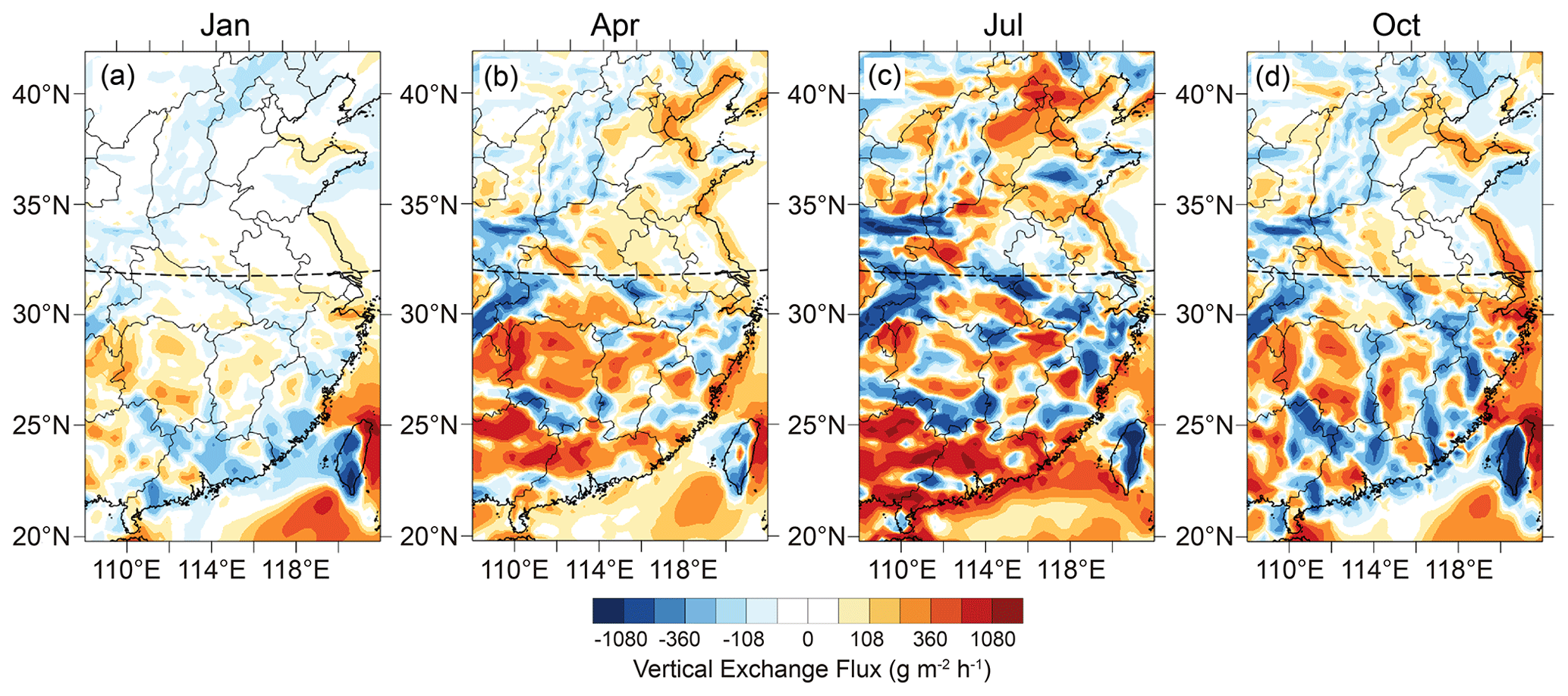
Figure 3 Spatial distribution of ABL–FT water vapour exchange fluxes in eastern China, averaged over 7 years for (a) January, (b) April, (c) July and (d) October. Dashed black lines mark the boundary between the northern (32–42^∘ N, 108–122^∘ E) and southern (20–32^∘ N, 108–122^∘ E) regions. Positive and negative fluxes (warm and cool colours) represent water vapour upward and downward transport at the ABL and FT interface.

3.1.2 Seasonal difference

Corresponding to Fig. 3, the spatial means of ABL–FT water vapour exchange flux and their seasonal evolutions for northern and southern regions are shown in Fig. 4. They are obtained by grid averaging in the ranges of 32–42^∘ N, 108–122^∘ E and 20–32^∘ N, 108–122^∘ E, respectively. Obviously, the exchange flux varies from season to season in both regions. For the northern region, winter and autumn (represented by January and October, respectively) are characterized by water vapour transport downward from the FT into the ABL, with the spatial mean fluxes of −15.6 and −18.8 g m⁻² h⁻¹ (1 g m⁻²  h${}^{-\mathrm{1}}=$ 10⁻³ mm h⁻¹) and the standard deviation of 3.6 and 8.6 g m⁻² h⁻¹ over 7 years. While in spring and summer (represented by April and July, respectively), the northern region as a whole presents an upward export of water vapour from the ABL to the FT, with the regional mean fluxes being 6.4 and 11.9 g m⁻² h⁻¹. They are characterized by more significant inter-annual variations than the exchange fluxes in the cold seasons. In the southern region, the water vapour vertical exchange is featured with ABL output in all seasons, with a winter minimum and a summer maximum. The mean upward fluxes vary greatly, showing levels 1 order of magnitude higher in April and July (99.1 and 115.51 g m⁻² h⁻¹) than in January and October (9.6 and 16.7 g m⁻² h⁻¹), accompanied by the larger standard deviation (50.4 and 68.4 g m⁻² h⁻¹). The notable interannual variability in the warm season may be related to the ENSO phenomenon, which will be discussed in the following section.

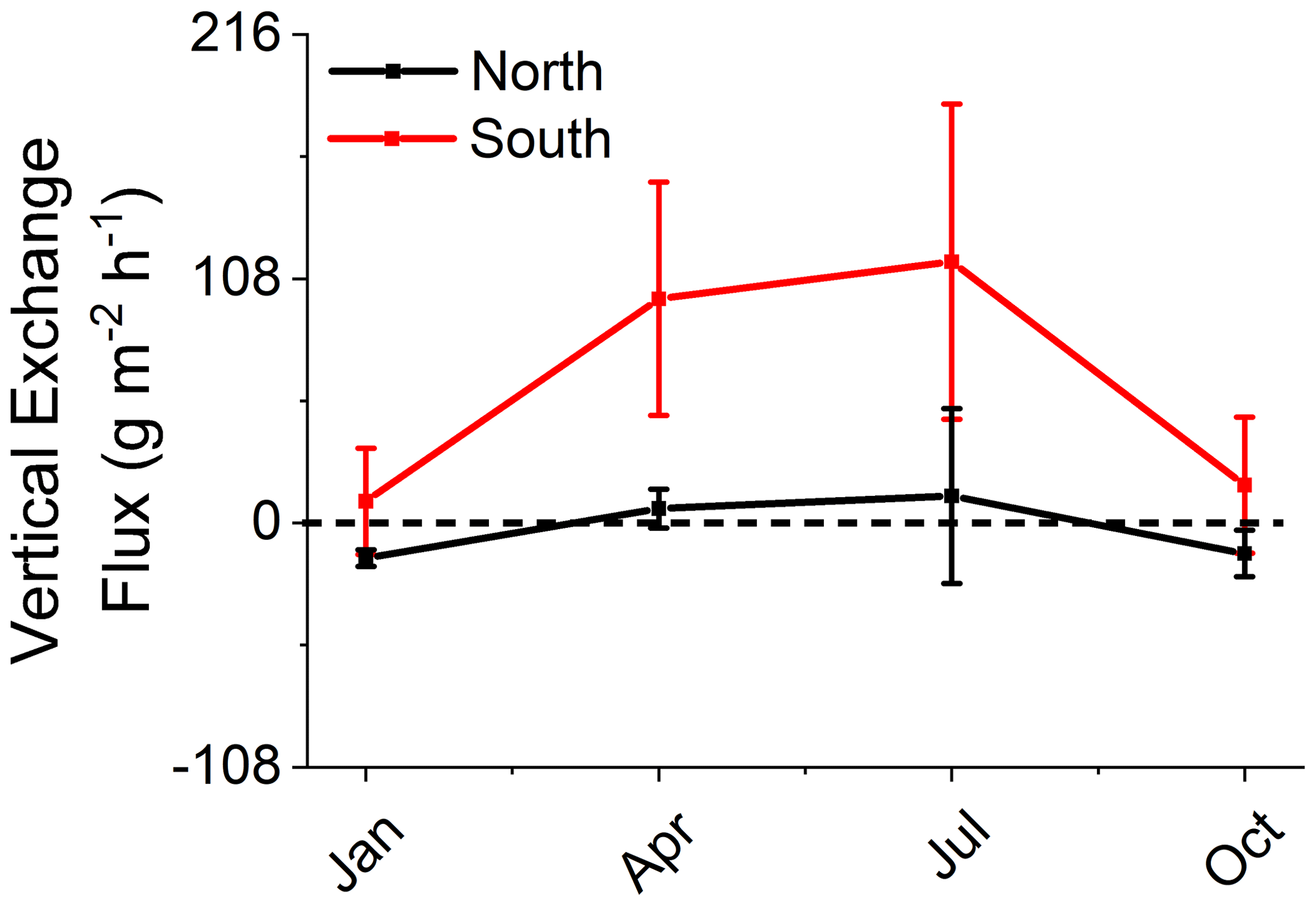
Figure 4 Seasonal variation of average ABL–FT water vapour exchange fluxes and their standard deviations over the northern region (32–42^∘ N, 108–122^∘ E) and southern region (20–32^∘ N, 108–122^∘ E) during 7 years. Positive and negative fluxes represent water vapour upward and downward transport between the ABL and FT.

In order to better understand the magnitude of water vapour exchange between the ABL and FT, we compare the transport flux with the surface evaporation rate (Table 1). It indicates the “emission intensity” of water vapour from the surface, which varies in different regions and seasons. The surface evaporation rates in the northern and southern regions have maximums in summer (122.4 and 194.4 g m⁻² h⁻¹) and minimums in winter (21.6 and 108.0 g m⁻² h⁻¹). Obviously, the evaporation in the north is weaker than that in the south; in particular, in winter, it is only one-fifth of that in summer. Consequently, for the northern region, during the cold seasons with the dry land surface, the ABL–FT water vapour exchange is downward, and the input flux is 37 %–72 % of the surface evaporation rate. Although the specific humidity decreases with height, counter-gradient transport still occurs reasonably because the ABL–FT exchange is a typically non-local mixing process (Stull, 1988; van Dop and Verver, 2001; Ghannam et al., 2017). This suggests the ABL is a net moisture sink of upper-layer FT air, which plays a role in maintaining water vapour within this layer. As surface evaporation intensifies in the warm months, water vapour is exported from the ABL in April and July, and the upward flux accounts for 10 % of the evaporation rate. In the southern region with relatively strong evaporation, the ABL water vapour is always transported upward to the FT. The output flux is about 10 % of the evaporation rate in January and October, and this ratio is as high as 60 %–80 % in April and July, indicating that the ABL acts as an effective water vapour source to the upper atmosphere.

Table 1 Comparison of ABL–FT water vapour exchange flux (g m⁻² h⁻¹, positive for upward, negative for downward) and surface evaporation rate (g m⁻² h⁻¹, positive for upward) in the northern and southern regions.

3.2 Main influential mechanism

As shown in Eq. (2), three physical terms contribute to the total ABL–FT exchange, i.e., the local temporal variation of ABL height (F_local), the horizontal advection across the spatial inclined ABL top (F_hadv) and the vertical motion through the ABL–FT interface (F_vadv). It is of interest to clarify the specific effects of these factors on water vapour vertical exchange and their seasonal characteristics. Results of the monthly mean and diurnal cycle over the 7 years are presented below, respectively.

The monthly mean results show that the term F_vadv is the most significant to total ABL–FT moisture exchange flux (Fig. 5, green bar). In the northern region, this term produces persistent downward flux (−19.5 to −44.7 g m⁻² h⁻¹, Fig. 5a), which substantially offsets the upward flux caused by the other two terms; therefore the ABL water vapour presents net input during cold months (i.e., January and October) and weak output in warm seasons (i.e., April and July). For the southern region, it induces small downward fluxes in January and October (−18.6 and −5.5 g m⁻² h⁻¹) while large upward flux in April and July (60.7 and 68.6 g m⁻² h⁻¹), which results in the total water vapour exchange as weak and strong output from the ABL during cold and warm months, respectively (Fig. 5b).

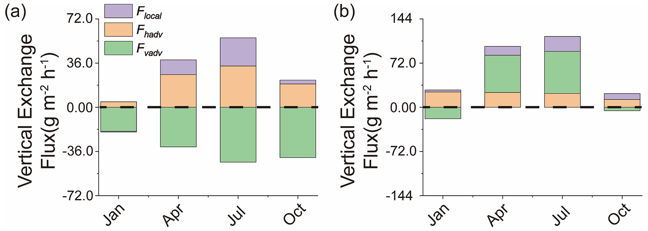
Figure 5 Contributions of three components (F_local, F_hadv and F_vadv) to the total ABL–FT water vapour exchange flux. Results are spatial mean over the (a) northern (32–42^∘ N, 108–122^∘ E) and (b) southern (20–32^∘ N, 108–122^∘ E) regions of eastern China, respectively. F_local: local temporal variation of ABL height (purple bar). F_hadv: advection across the spatial inclined ABL top (yellow bar). F_vadv: vertical motion through the ABL–FT interface (green bar). Positive and negative fluxes represent water vapour upward and downward transport between the ABL and FT. The y axis scales are different in (a) northern and (b) southern regions.

The upward/downward transport of water vapour caused by the term F_vadv depends on the direction of the vertical motion. The spatial distributions of the vertical velocity are presented in Fig. 6, accompanied by horizontal wind fields at the ABL top, as well as terrain heights. The upward motions usually occur on the windward of the mountains, while the descending velocities appear on the leeward side, in each season. This is attributed to the dynamic forcing of the terrain on seasonal mean winds. Due to the alternation of winter and summer monsoons throughout the year, the vertical motion pattern varies accordingly in four representative months (Fig. 6a–d). In the winter, the Siberian high invades from the northwest and forms strong northerly winds (Fig. 6e). In the northern region, the prevailing northwest airflows overcome the obstruction of Taihang Mountain and intensely descend on its leeward side (Fig. 6a). As the air migrates south, the dominant airflow deflects northeasterly (Fig. 6e), and the vertical motion manifests more upward velocities in front of the major mountainous region and more downward velocities behind these mountains (Fig. 6a). During the summer, southerly air flows dominate eastern China and gradually weaken from south to north (Fig. 6g). The southern region is characterized by obvious forced uplift on the windward side of the major mountains (Fig. 6c). The onshore airflow convergence of the prevailing southerly winds in coastal areas also produces upward motions (Fig. 6c). These factors are conducive to the vertical output of ABL water vapour in the southern region during warm months. The northern region is less invaded by the summer monsoon: only the eastern part of the NCP is affected by southerly winds to induce upward motion in the piedmont, while the western part is still dominated by westerly winds leading to systematic subsidence (Fig. 6c, g). The general patterns of vertical velocity fields provide an explanation for the water vapour exchange fluxes caused by the term F_vadv. It is noticed that, although the ABL–FT water vapour exchange fluxes in Fig. 3 are averages over 7 years, there is still obvious spatial heterogeneity. Smooth variations in both the mean wind field (Fig. 6e, h) and mean ABL height (Fig. S5) indicate these two factors are not related to the flux heterogeneity. But there are indeed discontinuous structures in the vertical velocity fields at the ABL top (Fig. 6a–d), which is significant to water vapour exchange flux. There can be smaller-scale secondary vertical motion that is stimulated when prevailing airflows encounter diverse terrains (Fig. S4). Multiscale dynamical interactions between complex terrain and synoptic processes should be of great significance to the water vapour exchange between the ABL and FT.

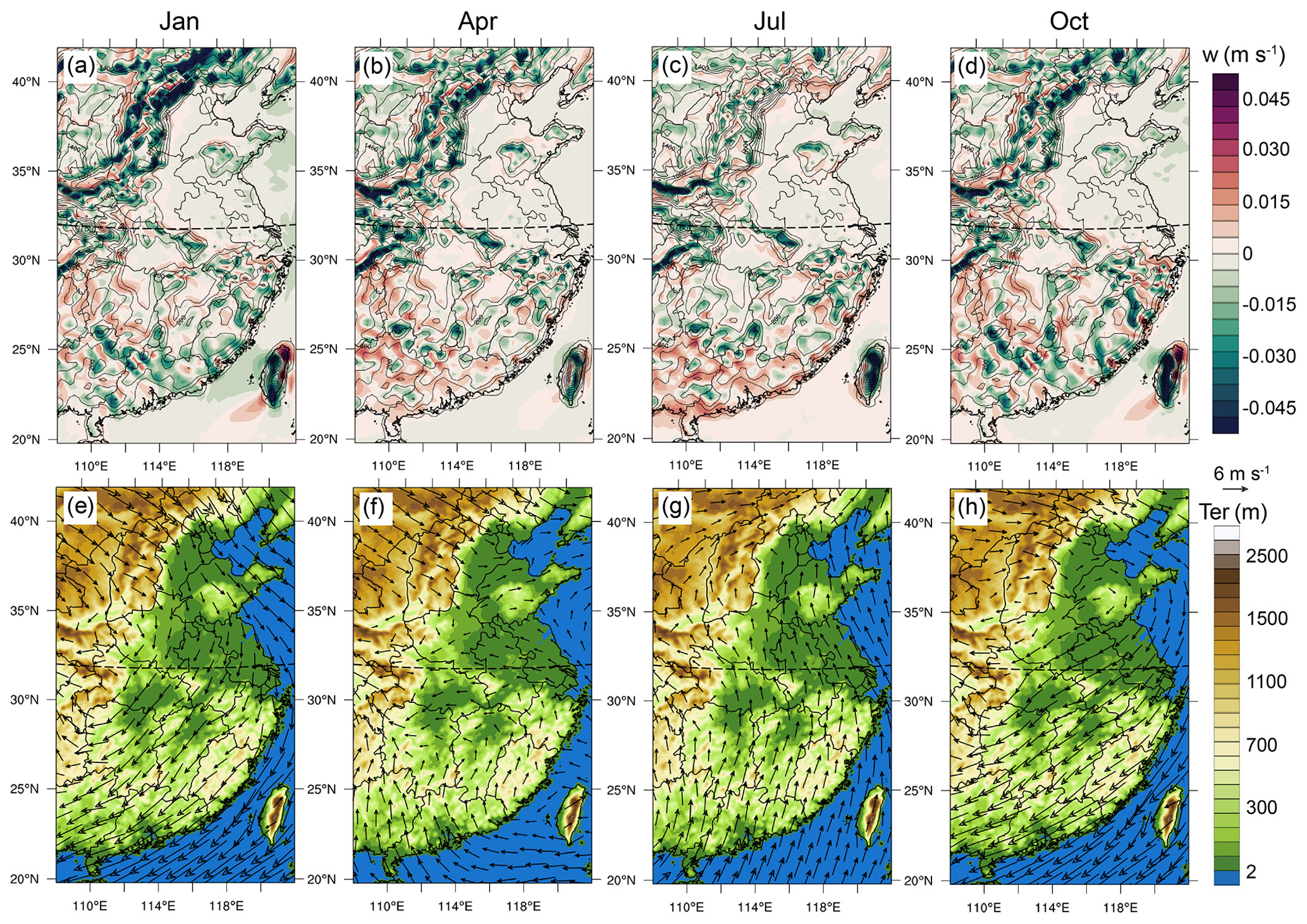
Figure 6 Spatial distribution of (a–d) vertical velocities at the ABL top and (e, h) terrain height superposed with horizontal wind vectors averaged over 7 years for January, April, July and October. Positive values represent upward motions, and the contours in (a–d) represent the terrain height. Dashed black lines mark the boundary between the northern (32–42^∘ N, 108–122^∘ E) and southern (20–32^∘ N, 108–122^∘ E) regions.

The horizontal advection term F_hadv tends to allow water vapour to be out of the ABL, and the magnitude increases in spring and summer (Fig. 5, yellow bar). This water vapour exchange component mainly occurs in the mountain–plain transition zone and the land–ocean boundary (Fig. S3e, h), where the ABL is unevenly distributed due to the heterogeneous surface properties (Fig. S5). During the warm season, the thermal difference is more obvious with the solar radiation strengthening and thereby with larger spatial variation of the ABL, especially in the northern region. This explains the seasonal variation of the water vapour exchange flux caused by the term F_hadv.

The temporal ABL height variation term F_local contributes relatively less to the total water vapour exchange (Fig. 5, purple bar). Noticeably, this average flux component is positive, being negligible in autumn and winter (0.7–3.3 g m⁻² h⁻¹) but becoming relatively pronounced in spring and summer (12.0–24.5 g m⁻² h⁻¹). This is inconsistent with the air mass exchange between the ABL and FT, in which the monthly average flux caused by this term is always insignificant because the ABL entrainment and detrainment of the air mass cancel each other out in a diurnal cycle (Jin et al., 2021). To understand more details of the term F_local in the ABL–FT water vapour exchange, the mean diurnal variation of the exchange flux is derived and shown in Fig. 7.

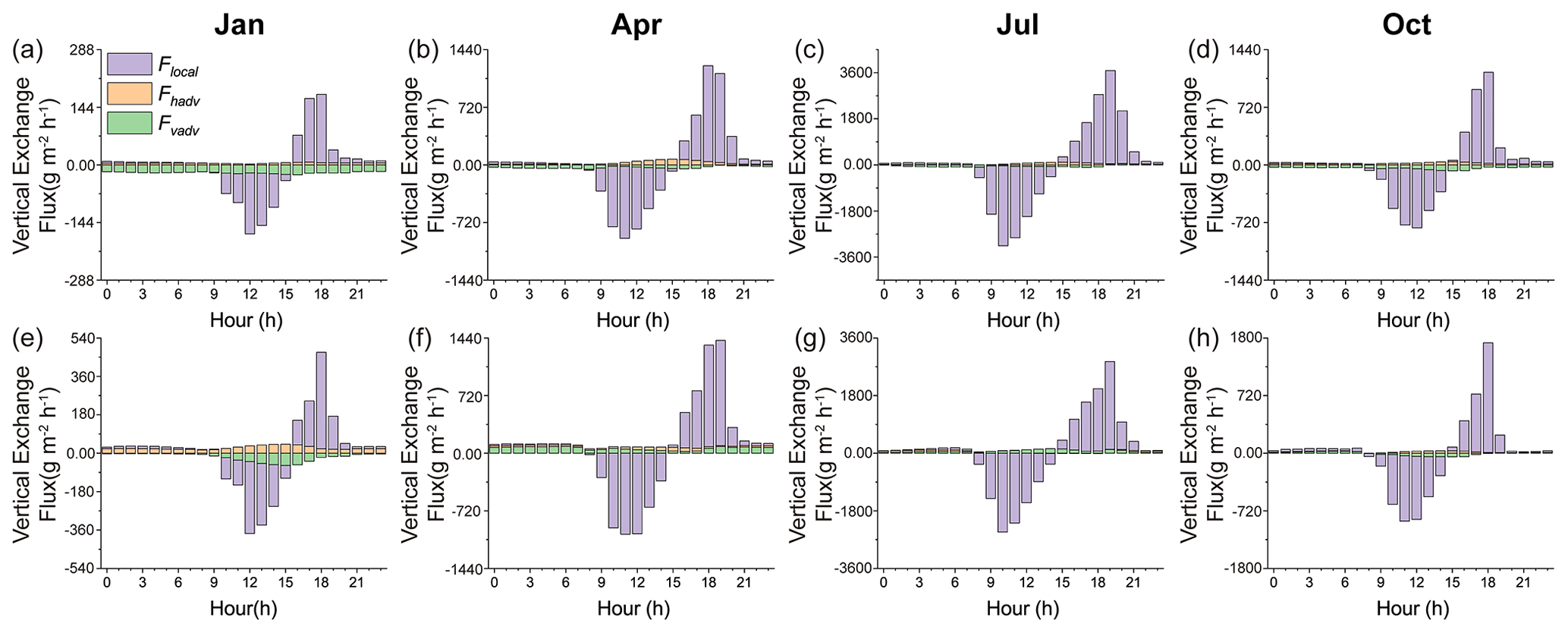
Figure 7 Diurnal variation of the three exchange flux components (F_local, F_hadv and F_vadv) over the (a–d) northern region (32–42^∘ N, 108–122^∘ E) and (e–f) southern region (20–32^∘ N, 108–122^∘ E) averaged for (a, e) January, (b, f) April, (c, g) July and (d, h) October. F_local: local temporal variation of ABL height (purple bar). F_hadv: advection across the spatial inclined ABL top (yellow bar). F_vadv: vertical motion through the ABL–FT interface (green bar). Positive and negative fluxes represent water vapour upward and downward transport between the ABL and FT. The y axis scales are different in different months and different regions.

At a first sight of the daily cycle, F_local is the absolutely dominant term in all seasons and both northern and southern regions (Fig. 7, purple bar), corresponding to the diurnal variation of the ABL height (shown in Fig. S6). When the unstable ABL develops in the morning, the water vapour in the residual layer is entrained into the ABL; while as the daytime ABL collapses in the later afternoon, a large part of water vapour is left aloft the newly formed stable ABL. Note that, unlike the air mass exchange at the ABL top, the water-vapour-entrained (input) flux is less than the output flux, especially in spring and summer. This difference can be attributed to the fact that the surface is, in general, a continuous evaporation source throughout a diurnal cycle. Turbulent mixing brings water vapour upward in the ABL depth and forms a net upward flux across the ABL top. This is also the reason why a larger magnitude of F_local exists in the warm seasons when there is stronger surface evaporation. Although the ABL temporal variation term F_local dominates the diurnal variation of the total ABL–FT moisture exchange flux, it contributes only a weak net output of water vapour in a monthly average flux, in comparison with the vertical motion term F_vadv, as mentioned above.

3.3 Interannual variability and its relation with ENSO

A climatic mean of the ABL–FT water vapour exchange over eastern China is presented above. Critically linked to the atmospheric water cycle, the exchange flux and its interannual variation are of great interest. It is well known that the atmospheric water cycle is significantly affected by the El Niño–Southern Oscillation (ENSO), which is a joint phenomenon of the ocean and the atmosphere appearing as a recurring anomaly of the sea surface temperatures in the tropical Pacific and a seesaw of sea level pressure anomalies between Tahiti and Darwin. The El Niño (warm phase) and La Niña (cold phase) are the two extremes of ENSO (Walker and Bliss, 1932, 1937; Kousky et al., 1984; Wolter and Timlin, 2011). Considerable work has been conducted on the relationship between ENSO and wet and dry variability, water vapour horizontal transport, and precipitation events (Diaz and Markgraf, 2000; Knippertz and Wernli, 2010; Felix Correia Filho et al., 2021). However, little is known about the ABL–FT water vapour exchange during ENSO events. Here we take July as the research object, the month with the largest variability (shown in Fig. 4), to investigate the interannual difference of ABL–FT water vapour exchange fluxes affected by the ENSO phenomenon.

The correlation between the water vapour exchange flux anomalies and the Niño-3.4 index during the study period (2011 and 2014–2019) is quantitatively calculated. The former (anomaly or variability) is derived from the difference of each year with the 7-year average, and the latter is obtained from https://psl.noaa.gov/gcos_wgsp/Timeseries/Nino34/ (last access: 20 October 2023), representing the average equatorial sea surface temperature across the Pacific from about the dateline to the South American coast (5^∘ N–5^∘ S, 170–120^∘ W), which is the most commonly used indices to define El Niño and La Niña event. The statistical result shows that there is a significant correlation between the two factors, with about 65 % of the grids meeting the 95 % confidence level. A positive–negative–positive triple distribution is presented in the correlation map (Fig. 8). On this basis, the sensitive areas are identified, in which the water vapour exchange fluxes are further analysed. The central region (28–35^∘ N, 108–122^∘ E) has the most obvious significance, where the proportion of significant grids is as high as 70 %. This area shows a negative correlation; i.e., the mean vertical output flux of water vapour is enhanced by about 57.6–151.2 g m⁻² h⁻¹ in cold-phase La Niña years (2011 and 2016, blue boxes in Fig. 9a) and vice versa in warm-phase El Niño years (2015 and 2019, red boxes in Fig. 9a), and the flux anomalies are close to 0 in neutral years (2014, 2017 and 2018, black boxes in Fig. 9a). In south (20–28^∘ N, 108–122^∘ E) and north (35–42^∘ N, 108–122^∘ E) areas with positive correlation coefficients, the trend is reversed. That is, the ABL moisture ventilation flux weakens 79.2–140.4 g m⁻² h⁻¹ in La Niña years and increases 108–194 g m⁻² h⁻¹ in El Niño years (figure not shown). This provides an explanation for the interannual variation of the water vapour exchange flux mentioned in Sect. 3.1.2.

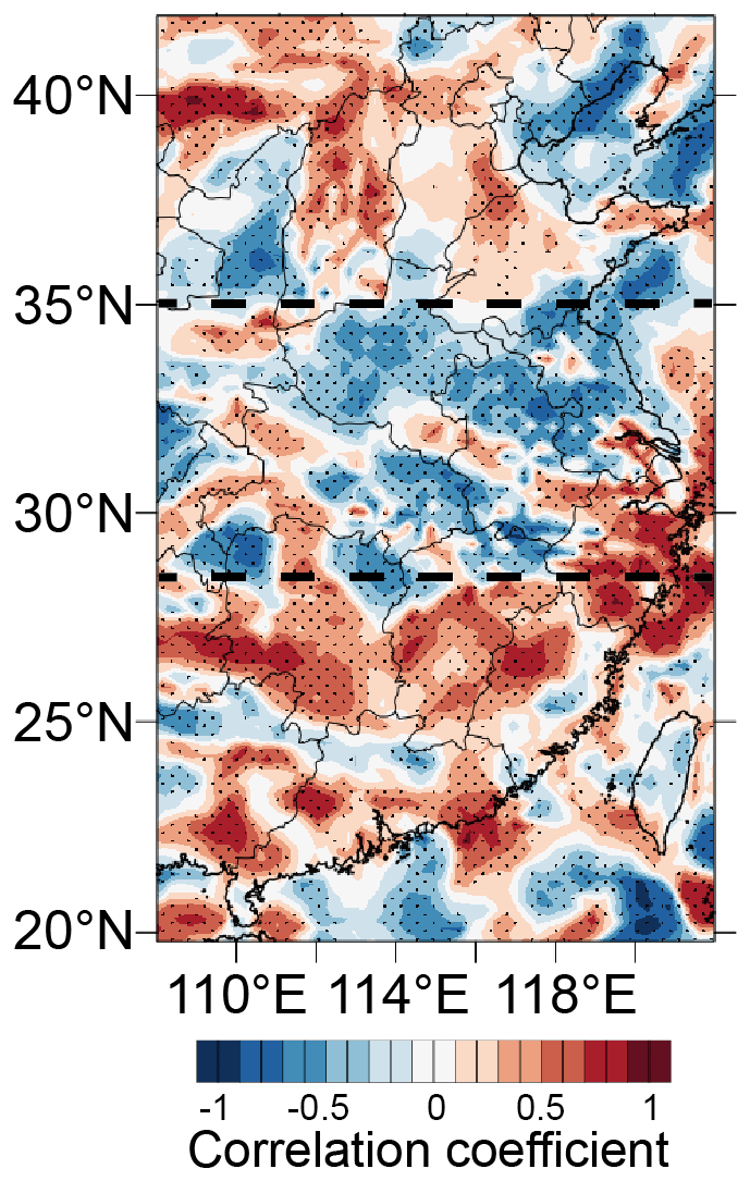
Figure 8 Spatial distribution of correlation coefficient between the water vapour exchange flux anomalies and Niño-3.4 index in July for 7 years. The dots indicate statistically significant grids, and the dashed black lines indicate the triple distribution.

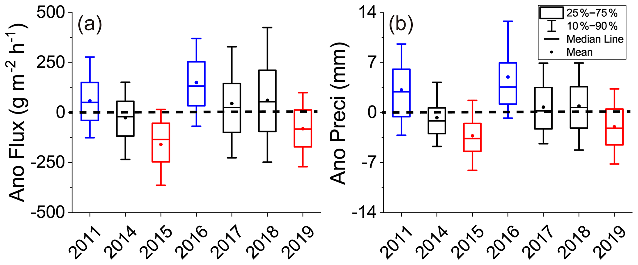
Figure 9 Anomalies of (a) water vapour exchange flux and (b) precipitation in July over the central region (28–35^∘ N, 108–122^∘ E; indicated in Fig. 8) during 2011 and 2014–2019. Blue, red and black indicate La Niña years, El Niño years and neutral years, respectively. Upper and lower sides of the box are the 75th and 25th percentile, and whiskers are the 90th and 10th percentile. Hollow squares and black lines in the box are mean and median.

In order to elucidate why the water vapour vertical exchange flux varies with ENSO, we further analyse three exchange components anomalies in El Niño and La Niña years (Fig. S7). Among them, the term F_vadv presents the most obvious correspondence with the correlation pattern (Fig. 8), demonstrating that vertical motion and water vapour content at the ABL top are crucial influencing factors. We select the central region (with the most significant correlation) for detailed analysis. As shown in Fig. 10, in La Niña years (represented by 2016), the upward vertical velocity strengthened, and the water vapour mixing ratio increased in the central area, while the opposite trend was observed in El Niño years (represented by 2015). This phenomenon is attributed to the stronger East Asian monsoon that brings more water vapour from the south and facilitates convergence to uplift during the cold-phase period of ENSO, while in the warm phase, the weaker southerly wind reduces water vapour transport and is not conducive to convergence within the ABL (Zhou et al., 2012; Xue et al., 2015; Gao et al., 2018), which explains the increase or decrease in ABL water vapour output affected by ENSO.

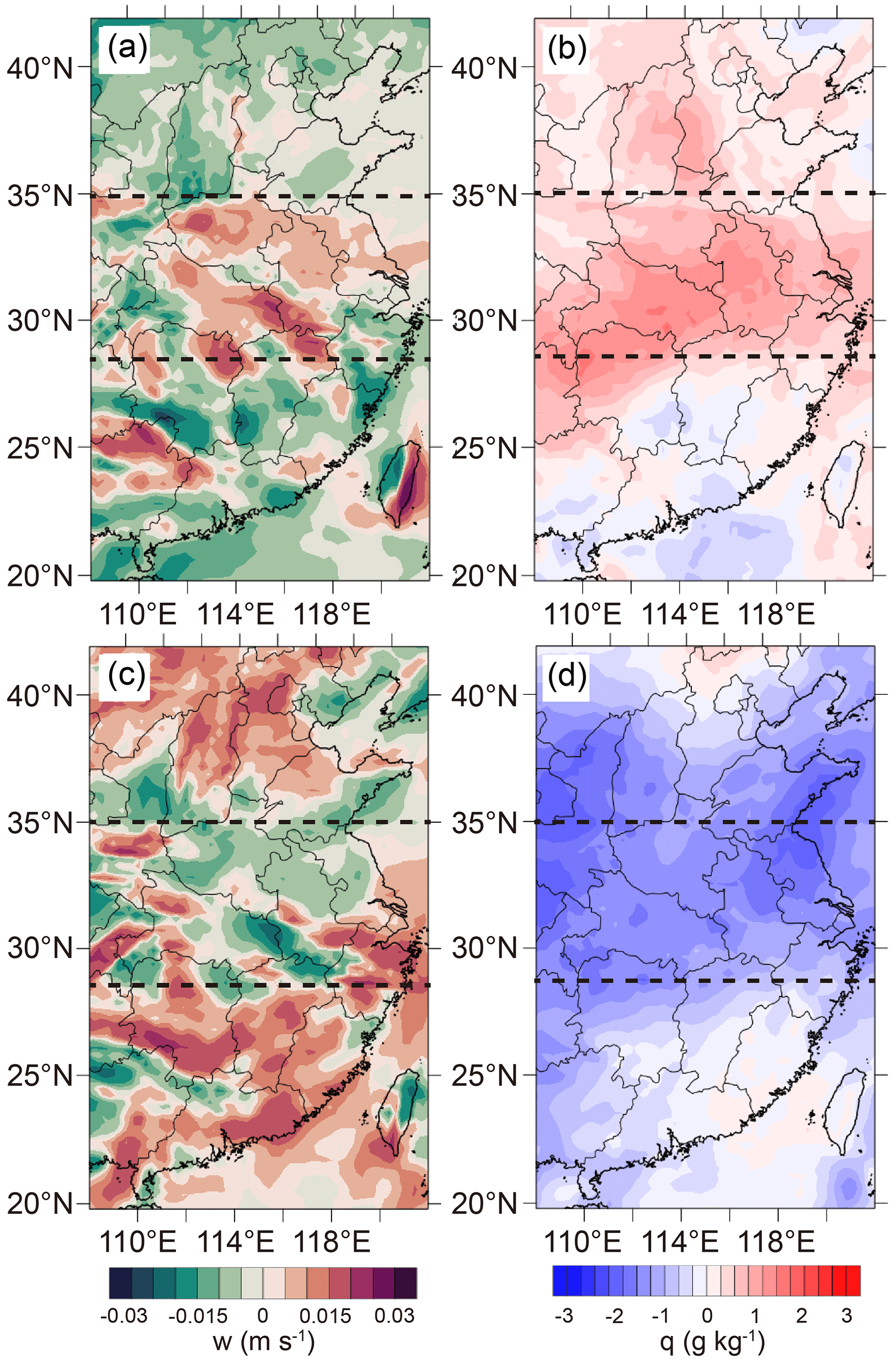
Figure 10 Spatial distribution of anomalies of vertical velocities (a, c) and water vapour mixing ratio (b, d) at the ABL top in July of (a–b) 2016 (La Niña year) and (c–d) 2015 (El Niño year).

Previous observation climatological studies have indicated that the summer precipitation anomalies in La Niña or El Niño years are characterized by a tripolar distribution over eastern China (Wang et al., 2020), similar to water vapour exchange flux anomalies revealed in this work. It is of interest to investigate the relationship between water vapour vertical exchange and precipitation under the influence of ENSO. Taking the central region (28–35^∘ N, 108–122^∘ E) as an example, the precipitation anomalies present a good correspondence with the variations of the ABL–FT water vapour exchange flux (Fig. 9). Specifically, precipitation increases (decreases) about 3.2–6.9 mm (2.8–3.5 mm) when the vertical output of water vapour intensifies (weakens) in La Niña (El Niño) years. That is, enhanced water vapour output flux from the ABL to the FT tends to produce increased precipitation and vice versa. These results imply that the upper-layer FT water vapour supplement from the ABL can also be a significant factor in changing regional precipitation, in addition to horizontal transport.

It should be stated that the above results are preliminary and rough, due to the limitations of the sample. The response of the ABL–FT water vapour exchange to ENSO and its impact on precipitation are complicated. The isolated patches in Figs. 8 and 10, as well as the box and whisker in Fig. 9 (being 75th–25th and 90th–10th percentile of the flux/precipitation anomalies), reflect the complex spatial variability over the research domain, which is not thoroughly analysed in the current work. Nevertheless, this general result points to an association among ABL–FT water vapour exchange, ENSO and extreme precipitation, which should be paid more attention in future research.

3.4 Discussion

The present results are based on numerical simulations. Although reasonable parameterization schemes are chosen according to sensitivity experiments, and the model performance is also evaluated by observational data, there are inevitable uncertainties in the modelled meteorological fields, which may directly affect the estimate of ABL–FT water vapour exchange flux. For example, the difference between the simulated ABL height and the observed value (∼ 70 and 120 m in winter and summer) brings ∼ 30 % uncertainty to the acquisition of vertical velocity at this level, which may affect the accuracy of the flux results in a similar magnitude. In addition, ignoring the turbulence term in this study may also reduce the accuracy of the results. Nevertheless, this work presents a general view of long-term and large-scale ABL–FT water vapour exchange over eastern China.

The water vapour exchange in the climatological sense presents a significant regional division of north and south China, due to their quite distinct climatic features. In addition to this general pattern, the spatial heterogeneity associated with the topographic distribution is also noteworthy. We try to sort out the vertical exchange fluxes of water vapour over the ocean, plain and mountain, roughly by altitudes below 0 m, between 0–200 m and greater than 200 m. The statistical results show that the ocean and plain are characterized by the upward output of water vapour from the ABL, while the mountainous regions are dominated by downward transport. This mode reflects the important role of the complex terrain in causing ABL–FT vertical exchange. As described in Sect. 3.2, the prevailing airflow is obstructed by the mountains to forcingly ascend on the windward and densely descend on the leeward slope, and then it decelerates and converges to induce upward motion when reaching the plain area. This vertical motion pattern makes the water vapour upward export from the ABL in the plain and downward transport in mountainous areas due to the intensity and effect of the leeward side subsidence being larger than that of the uplift in the windward side. For the ocean area, horizontal wind crossing the inclined boundary layer top is responsible for the ABL water vapour output, especially in the nearshore region. We admit the current analysis is preliminary, but it does indicate the characteristics of vertical exchange flux distribution with topography and the significance of the interaction between the mountains and sea and synoptic airflow. This finding suggests that topographic ventilation is not only caused by mesoscale circulations such as daytime upslope winds or sea breezes around mountains or coasts (Henne et al., 2004; Weigel et al., 2007) or convective activities on a relatively small scale or a specific time (Gonzalez et al., 2016; Dahinden et al., 2021). Dynamical forcing of terrain on seasonal airflow or synoptic winds is more essential, which induces vertical motion and leads to systematic water vapour exchange. The topographic-dependent feature of water vapour vertical exchange should also be of general meaning to other complex terrain regions around the world.

Moreover, the climatology of water vapour exchange flux between ABL and FT provides a quantitative background for investigating weather processes, radiation feedback and climate changes. Water vapour entering the FT may provide more latent heat to the energy flows and further affect synoptic systems. It is also involved in the radiative budget to influence climate. Previous model simulations and observations indicate that small yet systematic changes in the humidity of the upper atmosphere modulate the magnitude of the hydrological cycle and radiative feedback, including clouds and precipitation (Minschwaner and Dessler, 2004; Sherwood et al., 2010; Allan, 2012). Our results also demonstrate a notable relation between precipitation anomalies and ABL–FT water vapour exchange patterns. Based on the quantitative results in this study, the specific role of ABL–FT water vapour exchange in the Earth's energy flows and climate system might be studied further in the future.

4 Conclusions

In this study, we developed a climatology of water vapour exchange flux between the ABL and FT, based on 7-year meteorological modelling data. The ABL water vapour conservation method was used to estimate the vertical exchange flux across the ABL–FT interface. Spatial distribution and seasonal characteristics of the water vapour exchange were presented, and the influential mechanisms were analysed. The interannual difference was simply discussed through its variations with ENSO events. The major findings of this work are as follows:

1. The spatiotemporal distribution of the ABL–FT water vapour exchange was characterized by regional division and seasonal variation. During January and October in the northern part (32–42^∘ N), water vapour transport was downward to maintain ABL moisture, while in the southern region (20–32^∘ N) it was persistently exported to moisten the FT, with the output flux from 10 % to 80 % of the surface evaporation rate.

2. Vertical motion at the ABL–FT interface played a key role in the long-term (monthly or seasonal) average state of water vapour vertical exchange, which was caused by the dynamic forcing of the complex terrain on large-scale airflow. The temporal evolution of the vertical exchange flux over the course of 1 d was primarily driven by the diurnal cycle of the ABL height.

3. Interannual variability of ABL–FT water vapour exchange was related to ENSO. Their correlation was shown as a triple anti-phase distribution, with exchange strengthening in the central zone and weakening in the north and south in La Niña years (and vice versa in El Niño years). It was mainly attributed to the alteration of vertical velocity and water vapour content at the ABL top varying with ENSO phases. Moreover, this pattern presented a good correspondence to the distribution of precipitation anomalies.

This work is the first trial to quantitatively reveal the climatological state of ABL–FT water vapour exchange flux over eastern China. Though for this specific research domain, the method and results derived in the present study may provide reference to other regions of the world. Through this study, the moisture linkage between the Earth's surface and the upper-layer atmosphere is more clearly described. This may help us to obtain a better understanding of the atmospheric water cycle.