the Creative Commons Attribution 4.0 License.
the Creative Commons Attribution 4.0 License.
 | 27 Feb 2024
The Lagrangian Atmospheric Radionuclide Transport Model (ARTM) – sensitivity studies and evaluation using airborne measurements of power plant emissions
Dominik Brunner
Christiane Voigt
Alina Fiehn
Anke Roiger
Margit Pattantyús-Ábrahám
The Atmospheric Radionuclide Transport Model (ARTM) operates at the meso-γ scale and simulates the dispersion of radionuclides originating from nuclear facilities under routine operation within the planetary boundary layer. This study presents the extension and validation of this Lagrangian particle dispersion model and consists of three parts: (i) a sensitivity study that aims to assess the impact of key input parameters on the simulation results, (ii) the evaluation of the mixing properties of five different turbulence models using the well-mixed criterion, and (iii) a comparison of model results to airborne observations of carbon dioxide (CO2) emissions from a power plant and the evaluation of related uncertainties. In the sensitivity study, we analyse the effects of the stability class, roughness length, zero-plane displacement factor, and source height on the three-dimensional plume extent as well as the distance between the source and maximum concentration at the ground. The results show that the stability class is the most sensitive input parameter as expected. The five turbulence models are the default turbulence models of ARTM 2.8.0 and ARTM 3.0.0, one alternative built-in turbulence model of ARTM, and two further turbulence models implemented for this study. The well-mixed condition tests showed that all five turbulence models are able to preserve an initially well-mixed atmospheric boundary layer reasonably well. The models deviate only 6 % from the expected uniform concentration below 80 % of the mixing layer height, except for the default turbulence model of ARTM 3.0.0 with deviations of up to 18 %. CO2 observations along a flight path in the vicinity of the lignite power plant Bełchatów, Poland, measured by the Deutsches Zentrum für Luft- und Raumfahrt (DLR) Cessna aircraft during the Carbon Dioxide and Methane Mission (CoMet) campaign in 2018 allowed for evaluation of model performance for the different turbulence models under unstable boundary layer conditions. All simulated mixing ratios are of the same order of magnitude as the airborne in situ data. An extensive uncertainty analysis using probability distribution functions, statistical tests, and direct spatio-temporal comparisons of measurements and model results help to quantify the model uncertainties. With the default turbulence setups of ARTM versions 2.8.0 and 3.0.0, the plume widths are underestimated by up to 50 %, resulting in a strong overestimation of the maximum plume CO2 mixing ratios. The comparison of the three alternative turbulence models shows good agreement of the peak plume CO2 concentrations, the CO2 distribution within the plumes, and the plume width, with a 30 % deviation in the peak CO2 concentration and a less than 25 % deviation in the measured CO2 plume width. Uncertainties in the simulations may arise from the different spatial and temporal resolutions of simulations and measurements in addition to the turbulence parametrisation and boundary conditions. The results of this work may help to improve the accurate representation of real plumes in very unstable atmospheric conditions through the selection of distinct turbulence models. Further comparisons at different stability regimes are required for a final assessment of model uncertainties.
- Article
(8761 KB) - Full-text XML
-
Supplement
(4104 KB) - BibTeX
- EndNote


Atmospheric dispersion models (ADMs) are widely used by the scientific community and authorities. They are applied to a variety of problems, such as the study of the impact of pollutant emissions on air quality (Gariazzo et al., 2007; Stohl et al., 2007; Berchet et al., 2017; Lonati et al., 2022; Shupe et al., 2022) or the dispersion of radioactive discharges to the air (Chino et al., 2011; Connan et al., 2013; Draxler et al., 2015; Arnold et al., 2015), and they can operate at the full meteorological scale, ranging from the microscale (shorter than 1 km) to the mesoscale (1 km to 1000 km) up to the synoptic or global scale (larger than 1000 km).
The Atmospheric Radionuclide Transport Model (ARTM), analysed in this study, belongs to the class of models operating at the micro-β to meso-γ scales (approx. 0.5 to 20 km). It is a Lagrangian particle dispersion model (LPDM) designed for the dispersion of radionuclides from nuclear facilities under routine operation in the planetary boundary layer (PBL).
However, any ADM has to demonstrate its applicability to the system of study. The most important method to confirm this is validation (Kleijnen, 1995; Schlesinger et al., 1979). This includes (i) sensitivity analysis, which relates the model's response to variations in the model's input parameters, and (ii) a comparison with observations, revealing whether a model is an accurate representation of the system and whether simulation results are, to a certain degree, in agreement with observations (Kleijnen, 1995; Rao, 2005).
Concerning ARTM, Hettrich (2017) performed a sensitivity study to analyse the effect of input parameters (e.g. emission rate, source geometry, stability class, and particle number) on concentrations at selected locations near the ground. Hanfland et al. (2022) provided an overview of the physical basis and mathematical formulations of the model and presented a qualitative description of the influences of different input parameters on three-dimensional plume characteristics for a general simulation setup. However, both lack in quantifying sensitivities.
Here we expand these former studies with a more systematic and quantitative sensitivity analysis. Different sensitivity coefficients are calculated, which describe the dependence of the simulation output on the input parameter stability class (SC), roughness length (z0), zero-plane displacement factor (d), and source height (hs) within the whole simulated PBL and rank them according to their effects on the model output.
Publications presenting comparisons of ARTM's mixing ratio simulation results with measurements are rare. Hettrich (2017) compared ARTM simulation results with measurements at a few selected locations near the surface, showing discrepancies which are related to complex orography or local thermal-induced winds that are not covered by ARTM's wind field model TALdia. Martens et al. (2012) studied the influence of a single large building close to the source on the dispersion, showing that at distances larger than 4 km the influence decreases. These comparisons covered only a few atmospheric conditions and were limited to near-surface concentration measurements.
Brunner et al. (2023) presented an intercomparison of six different atmospheric transport models, including ARTM, with airborne in situ and remote sensing carbon dioxide (CO2) measurements, sampling the exhaust plume of the Bełchatów lignite power plant in Poland under very unstable atmospheric conditions (Fix et al., 2018). The data set comprises a considerable number of plume transects at different distances from the source and heights within the PBL, is characterised by a strong contrast between background and plume CO2 mixing ratios, and provides a three-dimensional description of the mixing ratio field. The spatial extent of the area covered by measurements is around the maximum domain size ARTM can tackle. In the Brunner et al. (2023) study, ARTM simulations are performed using the default turbulence model of ARTM version 2.8.0, including a workaround for meandering plumes because the simulated plume appeared to be too narrow under very unstable atmospheric conditions.
ARTM's dispersion depends on the turbulence model used (Hanfland et al., 2022), and since the three-dimensional data set facilitates further analysis of the model, we investigate whether the modelled plume could become more realistic by using different turbulence models. Two new turbulence models were implemented based on the ideas of Hanna (1982) and Degrazia et al. (2000) in addition to three built-in models of ARTM. The same workaround for meandering plumes based on the default turbulence model of ARTM 2.8.0, as primarily presented in Brunner et al. (2023), is also included in this study. Furthermore, all five turbulence models are evaluated concerning turbulence model characteristics and mixing efficiency and are compared with measurements.
The structure of this study is as follows: Sect. 2 gives a short description of the atmospheric dispersion model ARTM. Section 3 introduces several different sensitivity analysis methods and presents the sensitivity of typical model simulation outputs to key input parameters. Section 4 presents the five turbulence models and assesses their performance with respect to the well-mixed condition. Section 5 shows the comparison and evaluation of ARTM simulation results for the five turbulence models with the three-dimensional airborne data. Section 6 concludes the results of this paper.
The Atmospheric Radionuclide Transport Model is an LPDM developed specifically for the dispersion of radioactive emissions from nuclear facilities in an area of typically 10 km × 10 km. Its purpose is to provide annual activity concentration fields in the area around nuclear facilities under routine operation in slightly structured non-urban terrain, which are used in a follow-up step to calculate the additional exposure of the population (Hanfland et al., 2022).
The dispersion model propagates numerical particles representing radioactive tracers in space and time according to wind and turbulence fields obtained by a diagnostic approach. Meteorological data from measurements in the vicinity of the nuclear facilities are used to calculate a mass-conserving diagnostic wind field. The turbulence is obtained by a Markov process, which uses wind speed fluctuations and Lagrangian correlation times as input parameters, both depending on the Obukhov length as a turbulence parameter. This static diagnostic approach employed by ARTM is similar to that of, for example, SWIFT/micro-SWIFT or CALMET (Cox et al., 2005; Moussafir et al., 2004; Scire et al., 1998) but differs from other larger-scale LPDMs, such as FLEXPART, STILT, NAME, or HYSPLIT, which use prognostic meteorological fields from a numerical weather prediction model to drive the particle propagation (Hanfland et al., 2022; Lin et al., 2003; Stohl et al., 2005; Ryall and Maryon, 1998; Draxler and Hess, 1998). The advantage of this static diagnostic approach is its high computational efficiency with typical applications from 10 km to a few hundred kilometres for horizontal extent, depending on the number of meteorological measurement locations and the terrain (Ratto et al., 1994). Since ARTM works with one single meteorological measurement location, its simulation domain can horizontally extend to up to a few tens of kilometres depending on the terrain. The simulation domain is divided into grid cells for which the average activity concentration for the whole simulation period is calculated. A detailed model description is given in Hanfland et al. (2022).
Sensitivity analysis (SA) is a method to study the model's response to variations in input parameters in a systematic way, and it may answer the following questions. How does the uncertainty in input parameters influence the model output? Which parameters require additional research in order to reduce output uncertainty? Which parameters are the most significant or insignificant for the model's output? And does the model behave as expected when varying a certain input parameter (Hamby, 1994; Frey and Patil, 2002; Rao, 2005; Saltelli et al., 2008)? SA methods are either local or global depending on the sampled input parameter space (Saltelli et al., 2008; Morio, 2011; Zagayevskiy and Deutsch, 2015).
The results of the methods may differ depending on the shape of the input parameter space. Thus, the application of several methods is recommended (Iman and Helton, 1988; Hamby, 1995). In this work, several different local and global SA methods are therefore applied to ARTM 2.8.0 using its default turbulence model (Hanfland et al., 2022). A description of the turbulence model for unstable atmospheric conditions is given in Sect. 4.1. The application of several SA methods provides a comprehensive assessment of the response of ARTM to different input parameters.
3.1 Local sensitivity analysis methods
Local SA focuses on one single point in the input parameter space. The output of a model is represented by , where the random variables Xi with denote the different input parameters. The representations (or values) of Xi are denoted with xi. The input parameters Xi are varied one at a time, while all the other parameters are held constant at their reference values . This local SA approach is similar to estimating the partial derivative and characterises the effect of the input parameter Xi on Y at one reference point (Morio, 2011).
3.1.1 Sensitivity index
The sensitivity index described by Hoffman and Gardner (1983) uses the parameters at the reference point where each parameter is varied one at a time by their full range. The sensitivity index is calculated as
where Yi,max (min) indicates the maximum (minimum) output value. The sensitivity index is a value between and gives the fraction of output variation caused by the varied input parameter (Hamby, 1994).
3.1.2 One-at-a-time sensitivity measure
The one-at-a-time sensitivity measure calculates the variation in the model output normalised to the largest output variation ΔYmax that had been observed for the different input parameters. Starting from the default parameter set, the parameters are varied one at a time by a percentage α. The sensitivity coefficient for the input parameter Xi is calculated as
where (Link et al., 2018). In this work the percentages ± 25 % and ± 50 % are used for α. is a value between , where unity identifies the input parameter with the biggest effect on the model output Y.
3.2 Global sensitivity analyses
Global SAs sample the whole input parameter space, which leads to a broader representation of the sensitivity compared to local methods but also increases computation time. A general discussion about global SAs can be found in Saltelli et al. (2008).
3.2.1 Sobol′ indices
The variance-based Sobol′ indices use variance decomposition to calculate indices of different orders (Sobol', 1993). Usually, only two key Sobol′ indices are determined: the first-order index Si and the total-effect index STi.
For the first one, the conditional expected value of the model output with a constant value of Xi and varying values for every other input parameter X∼i is computed. For different realisations of Xi, reflects the variance of the model output Y originating from a variation in the input parameter Xi. The first Sobol′ index is then given by
where V(Y) is the unconditional variance of the output where all Xi values are varied. cannot be larger than V(Y), and thus for the sensitivity coefficient is valid. This index is called the first-order sensitivity index as it does not take higher-order effects (i.e. interactions between different input parameters) into account (Saltelli et al., 2008).
The second index considered here is the total-effect index. It takes higher-order terms into account, which might be important depending on the model. The total effect is calculated as
where , Xi+1, …, Xk)]≤V(Y) is the total variance of all input parameters except Xi. As the first-order index, this total-effect index is a value between 0 and unity, where a value of 0 indicates no influence of Xi on the output Y, while unity indicates a strong influence (Saltelli et al., 2008). A comprehensive description of the method is given by Saltelli et al. (2008).
For the analysis presented here, the Python library SALib (Herman and Usher, 2017) is used for the quasi-random sampling with low discrepancy in the input parameter space, after Joe and Kuo (2008), as well as for the calculation of the Sobol′ indices. It furthermore allows for the estimation of the 95 % confidence intervals (Herman and Usher, 2021).
3.2.2 δ method
In comparison with the Sobol′ indices, the δ method takes the complete density distribution of the model output into account, which ensures the conservation of all the information of the output density distribution (Borgonovo, 2007). The probability density function of Xi is denoted . The sensitivity coefficient δi for the input parameter Xi is calculated using the marginal density distribution of the input parameter and the difference between the unconditional and the conditional density functions fY(y) and of the model output with fixed representation Xi=xi as (Borgonovo, 2007)
δi represents the total effect of an input parameter Xi on Y. It can take a value between 0 and unity (), where 0 means that the output is independent of Xi (Plischke et al., 2013). The same library (SALib; Herman and Usher, 2017) was used to apply the δ method and estimate the 95 % confidence interval.
3.3 Model setup for sensitivity analyses
For the SA a simple model setup with a single source and constant wind was chosen. Figure 1 illustrates the simulation domain with the plume sampled at a height of 20.5 m above ground level (a.g.l.). The simulation domain has an extent of 10 km × 1.5 km × 1.5 km in the x, y, and z directions. The x direction is defined in a west–east orientation and the y direction in a north–south orientation. The domain is divided into grid cells with a horizontal resolution of 50 m. Vertically, the 1.5 km high simulation domain is divided into 19 levels of varying thickness gradually increasing from the lowest layer (3 m thick) to the top simulation layer (300 m thick). The level thicknesses are shown in Table S1 in the Supplement. The point source is located at the coordinates (x = 25 m; y = 25 m). The vertical position is varied during the SAs. A constant westerly wind (270°) was used for the entire simulation period of 24 h with a velocity of 1 m s−1 at 10 m height. In order to focus on the evolving dispersion pattern, the topography is assumed to be a flat surface. The gaseous krypton isotope 85Kr with a decay constant of λdecay = 2.05 × 10⁻⁹ s−1 was used as a tracer. This results in a decay of less than 0.02 % within the simulation period and can therefore be neglected. The emission source is represented as a source with a constant activity rate of 1 Bq s−1.
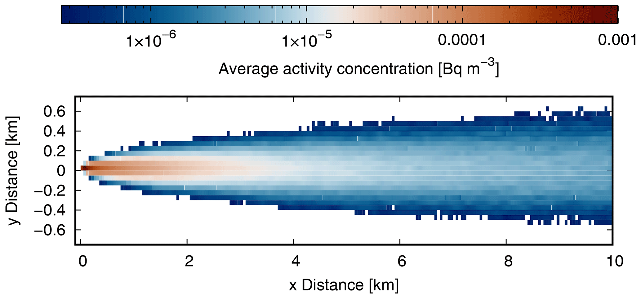
Figure 1The x–y plane of the simulation domain for the sensitivity analyses with the activity concentration at a height of 20.5 m. The generic plume is simulated for SC (neutral), z0 (0.5 m), d (6), and hs (20 m) with a wind speed of 1 m s−1 from the west at 10 m height and an emission rate of 1 Bq s−1. The activity concentration distribution in Bq m−3 is given in a logarithmic scale.
Table 1Input parameters and their values and ranges. The default parameters for local SAs are marked with ∗.
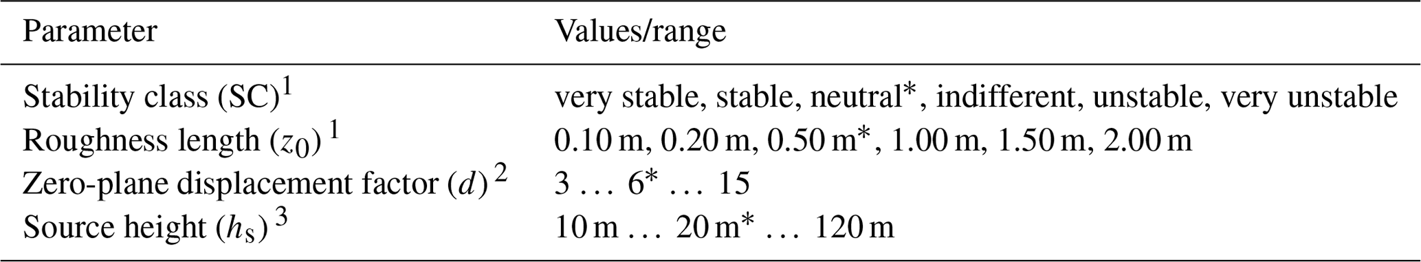
1 For the global SAs the given values are sampled. 2 For the global SAs the values are sampled continuously within the range. 3 For the global SAs the values are sampled with a resolution of 1 m within the range.
The input parameters stability class SC, roughness length z0, zero-plane displacement factor d, and source height hs are assumed to be the key parameters of ARTM. The zero-plane displacement d0 depends on d as . When using d instead of d0 the input parameters for the SA are independent. This allows for the analysis of the unbiased effects of input parameter variations. These parameters and their ranges are summarised in Table 1. Only a discrete set of six SCs is allowed in ARTM. The range of z0 values allowed by ARTM is limited to the roughness lengths that correspond to typical land covers in the vicinity of German nuclear facilities. German authorities recommend a value of d=6 for the zero-plane displacement factor (TA Luft, 2002; VDI 3783 part 8, 2017). The range for the variation in d is centred on this value and limited to forest canopy heights typical of mixed forest (Lang et al., 2022). In Table 1, the parameter values for the reference point for the local SAs are marked with a * symbol. For global sensitivity analyses, the whole parameter range is sampled.
The target quantities of the SAs are two important characteristics of the plume: (i) the plume volume, which is a measure of the tracer dispersion and is closely linked to the maximum mixing ratio, and (ii) the distance between the location of the maximum activity concentration and the source position at ground level, which is of special interest for radiation exposure assessment.
Table 2Sensitivity coefficients of local and global sensitivity analyses for the plume volume and for the distance between the source and the maximum concentration at the ground level. For the Sobol′ indices (Si and STi) and the δ method (δi) 95 % confidence intervals are given as well. Coefficients with very large relative confidence intervals are marked with ∗, and coefficients of one method, which cannot be distinguished within their confidence intervals, are marked with †.
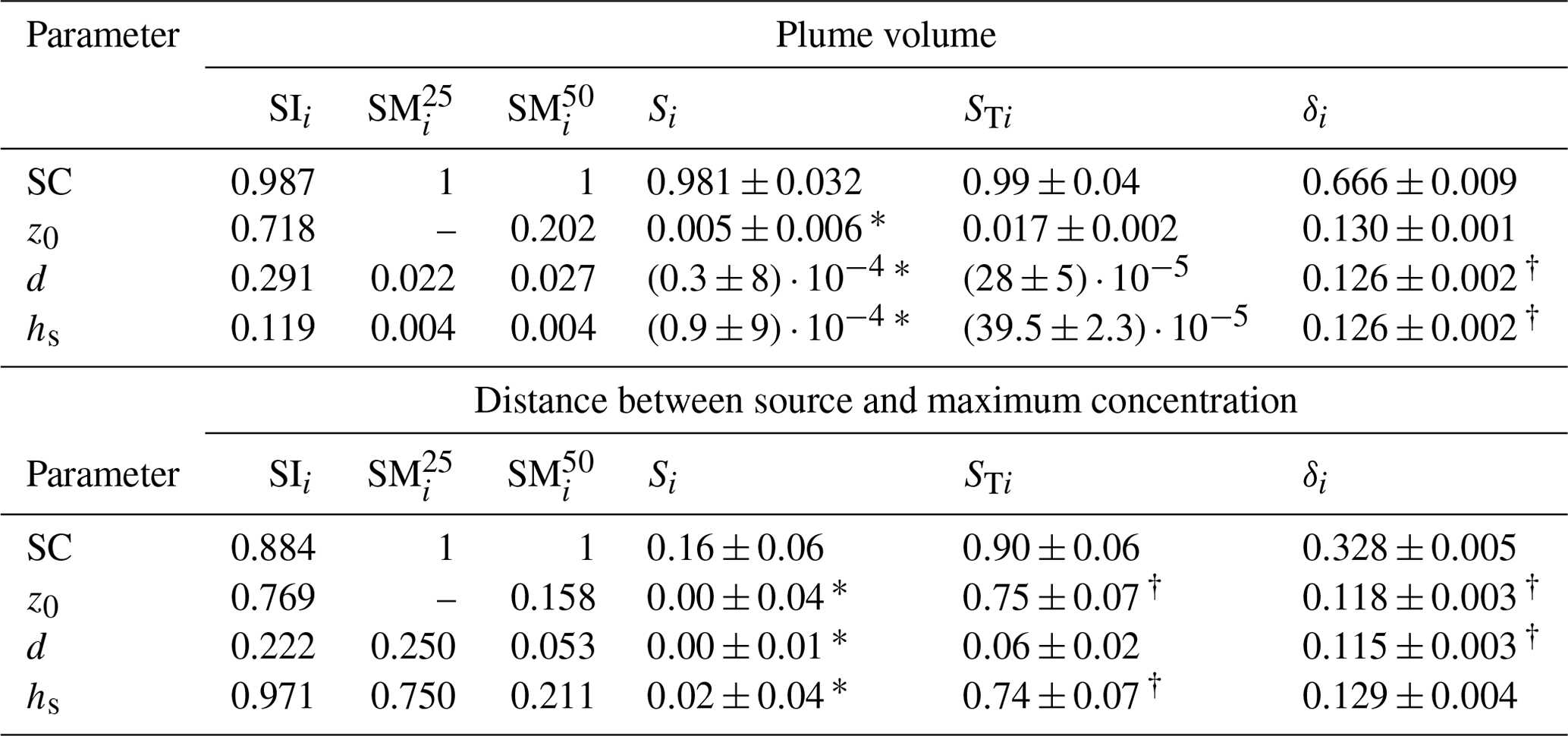
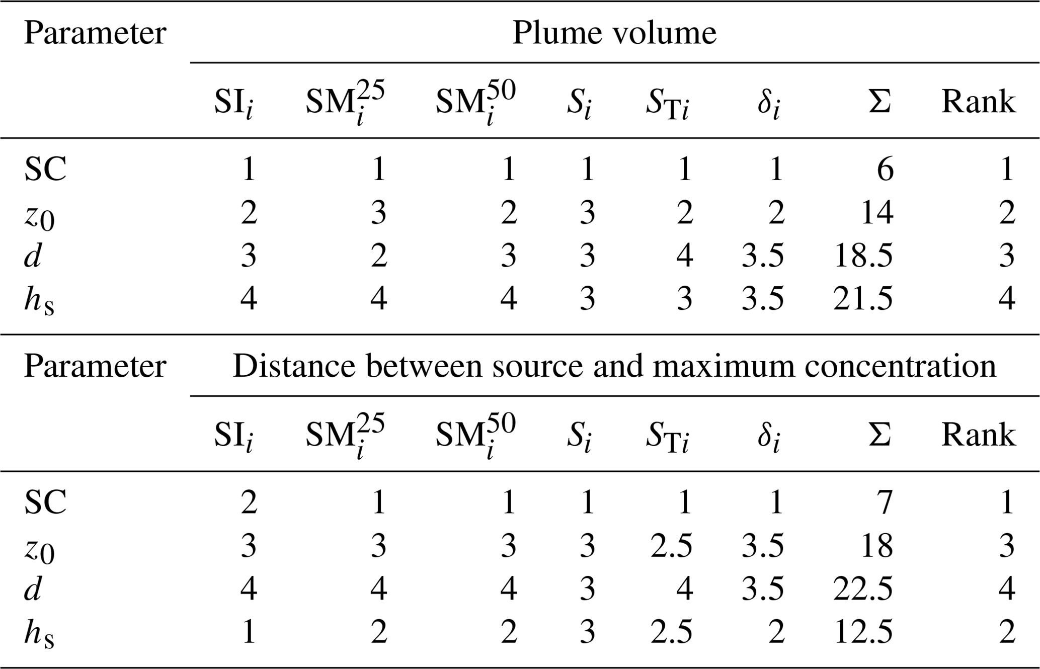
Table 3Ranking of the influence of the input parameters on the plume volume and on the distance between the source and the maximum concentration at ground level for local and global sensitivity analysis methods.
3.4 Results of the sensitivity analyses
The results of the calculations of the local and global sensitivity coefficients are summarised in Table 2. Concerning the plume volume, all SA methods compute the highest SA coefficients for the stability class. Although less prominent, this is also observable for the distance between the source and maximum concentration at the ground level, except for sensitivity index SIi.
For no value can be calculated because a variation of ± 25 % from the reference roughness length value does not lead to a change in the categorial z0 value. For the other parameters, the two different ranges of variation (α=25 and α=50) for provide valuable additional information. For example, it can be seen from Table 2 that the deviations between the coefficients of and are small for the plume volume, while they are large for the distance between the source and the maximum concentration. The influence of the input parameters seems to be rather linear for the plume volume but highly non-linear for the distance between the source and maximum concentration at the ground.
For the global SA methods, both target quantities show a distinct importance not only of first-order (direct influence of one single input parameter) but also of higher-order (including interactions of two or more input parameters) effects. A small difference between Si and STi shows a large first-order effect, as can be seen for the plume volume. On the contrary, a large difference reveals a small first-order effect rather than a higher-order effect, as can be seen for the distance between the source and maximum concentration at ground level. This agrees with the conclusions that can be drawn from the δi coefficients. The sum of the sensitivity coefficients for the plume volume indicates that the effects of variation in the input parameters on variation in the plume volume are separable; i.e. interactions between input parameters play a minor role. For the distance between the source and maximum concentration, the sum of the sensitivity coefficients indicates the important role of cross-interactions between the input parameters (Borgonovo, 2007). Contrary to the findings of the Sobol′ indices that some input parameters have negligible influences, the δ method suggests that the output characteristics are sensitive to all parameters. This difference could be due to the different amounts of information processed by the two methods. While the Sobol′ indices compare conditional and unconditional variances of the output distribution, the δ method takes the entire output distribution into account.
Some of the global SA coefficients have very large relative confidence intervals and cannot be distinguished from 0 (marked with ∗). Others cannot be distinguished from each other within their confidence intervals (marked with †). Increasing the sample size of 24 576 further would be necessary to get smaller confidence intervals, but this would also increase the computation time (Herman and Usher, 2021).
Based on the coefficients from Table 2, the input parameters were ranked according to their importance as summarised in Table 3. The rankings obtained for the individual SA methods differ not only for the two target quantities but also between different methods. The overall ranking, which is simply computed as the sum (Σ) of the different methods, is provided in the second-last column.
The most unambiguous result is that all SA methods show the plume volume to be the most sensitive to the SC. The ranks for the other input parameters, in contrast, are not the same. At this point we want to mention that the ranking of given in Table 3 is the average of all possible rankings for this method when taking into account that there is no coefficient for . The rankings of the remaining local SA methods, SIi and , are in agreement with each other for the plume volume, while the rankings of the global SA methods disagree. Compared to the rankings for the plume volume, those for the distance between the source and maximum concentration at the ground level are less uniform.
The overall rankings for both target quantities differ from each other, which emphasises that different target quantities are not necessarily sensitive to the same input parameters. Both target quantities are the most sensitive to the SC, which is thus a potential source of high uncertainty. The source height hs has little influence on the plume volume, but it is the second most important parameter for the distance between the source and maximum concentration at the ground level.
In LPDMs the turbulent motion is described via a Markov chain approach in the form of a Langevin equation (Lin and Gerbig, 2013). ARTM uses the wind speed fluctuation σ and Lagrangian correlation time TL as input parameters for this Markov chain approach (Hanfland et al., 2022). The turbulence model specifies these two parameters and thus influences the tracer dispersion and hence the simulated mixing ratio field (Katharopoulos et al., 2022).
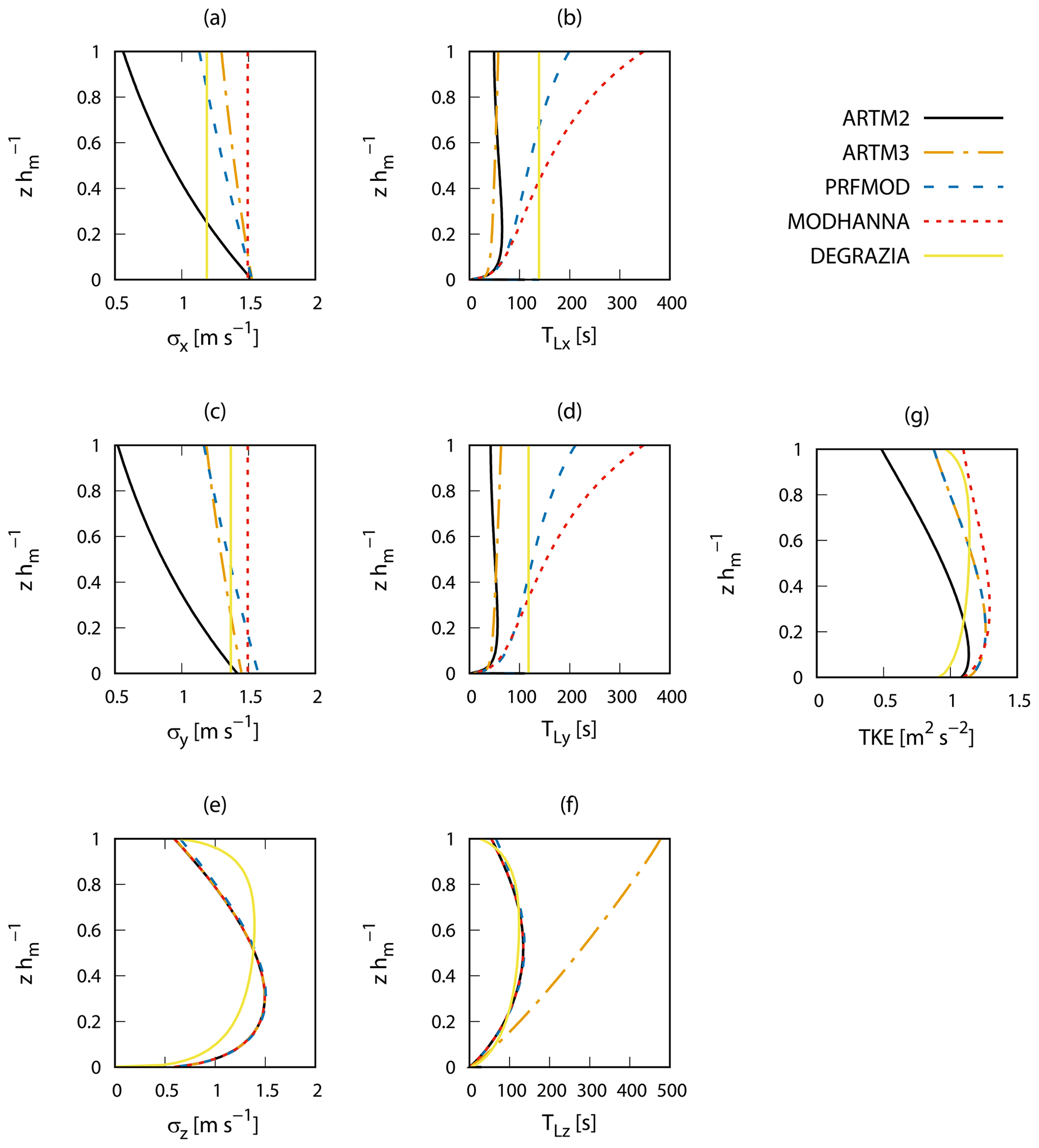
Figure 2Vertical profiles of the model characteristics of the five turbulence models, ARTM2, ARTM3, PRFMOD, MODHANNA, and DEGRAZIA, under very unstable atmospheric conditions. Wind speed fluctuation σ: (a) along-wind direction σx, (c) crosswind direction σy, and (e) vertical direction σz against the normalised height (normalised to the boundary layer height). The corresponding Lagrangian correlation time TL is shown in (b), (d), and (f). The turbulent kinetic energy per unit mass TKE is shown in (g).
4.1 Description of turbulence models
The turbulence model implemented in ARTM 2.8.0 as the default model is not widely used in the scientific community. Besides this, it has been reported by Janicke and Janicke (2011) that it sometimes underestimates plume dispersion. Therefore, they introduced a modified turbulence model, leading to stronger dispersion, which can optionally be activated in ARTM. In 2022, the new version (3.0.0) of ARTM was released. It implements a new turbulence model according to the Association of German Engineers (VDI) guideline VDI 3783 part 8 (2017). All three models deviate from the model suggested by Hanna (1982), which is quite widely used and thoroughly tested against tracer release experiments. However, in this model the turbulence may abruptly change between SCs. To overcome this issue of discontinuity, Degrazia et al. (2000) proposed a continuous description of the turbulence throughout all atmospheric conditions. Since the measurement data set used for the comparison of simulations and observations was collected under unstable atmospheric conditions, the following analyses focus on unstable stratification. The wind speed fluctuation σ and the Lagrangian correlation timescale TL of the five turbulence models are presented in Eqs. (6)–(26) for unstable stratification, and their profiles are displayed in Fig. 2. For the following quantities we define the x components along the average horizontal wind direction, the y components perpendicular to it in the horizontal plane, and the z components in the vertical direction. Although the zero-plane displacement is used in ARTM (GRS, 2015) to displace the wind profile vertically to account for the influence of obstacles, for the sake of simplicity it is not included in the following equations.
The first model, the default boundary layer model (BLM) of ARTM 2.8.0, was initially suggested by Kerschgens et al. (2000) and is based on the work of Lenschow et al. (1980), Panofsky et al. (1977), Hicks (1985), and Gryning et al. (1987). It describes profiles for the wind speed fluctuations as
and
where u∗ is the friction velocity, hm is the mixing layer height, κ=0.4 is the von Kármán constant, L is the Obukhov length, and z is the height above ground level (VDI 3783 part 8, 2002; Hanfland et al., 2022). This model is called ARTM2 in the following.
The second turbulence model available in ARTM is based on ARTM2 with a modification in the exponents and in the prefactor of the crosswind component as follows (Janicke and Janicke, 2011):
and
This model leads to wider plumes and is called PRFMOD in the following.
In addition to the two previous models, we added a turbulence model to ARTM based on ARTM2 modified with formulations used in other ADMs (Stohl et al., 2005). This model uses σz from ARTM2 given in Eq. (8), but the horizontal wind speed fluctuations
are equal to the equations suggested by Hanna (1982). The aim of this modification is to increase the turbulent kinetic energy and to analyse the effect of the horizontal wind speed fluctuations on the dispersion. In the following, this model is called MODHANNA.
The Lagrangian correlation times of the three models are given according to Kolmogorov's theory as (Luhar and Britter, 1989)
with the Kolmogorov constant C0=5.7 and the dissipation rate of the turbulent kinetic energy
The fourth model is the default model of the new version of ARTM (3.0.0) with the wind speed fluctuations given as (VDI 3783 part 8, 2017)
and
The Lagrangian correlation timescales are calculated via the turbulent diffusion coefficient Ki as
with
for the horizontal component j and
for the vertical component (VDI 3783 part 8, 2017). This model is called ARTM3 in the following.
We implemented a fifth model, which, in contrast to the previous four turbulence models that are based on similarity theory, is based on the spectral distribution of the turbulent kinetic energy of the boundary layer and was presented by Degrazia et al. (2000). For very unstable boundary conditions the wind speed fluctuations are given as
and
with the Lagrangian correlation time
where li is the Lagrangian correlation length given as
and
In this work this turbulence model is denoted as DEGRAZIA.
The turbulent kinetic energy per unit mass is determined as (Stull, 1988)
4.2 Evaluation of turbulent mixing
The degree of preservation of well-mixed conditions is a key quality indicator for any LPDM, similar to the preservation of mass in an Eulerian model. It tests whether an initially uniform distribution of a tracer in an incompressible flow remains uniform as postulated by the second law of thermodynamics (Sawford, 1986; Thomson, 1987; Lin and Gerbig, 2013; Bahlali et al., 2020). Exactly fulfilling this criterion is challenging, but it is important to quantify the degree of deviation from this ideal behaviour to judge the magnitude of systematic model biases and whether these biases are acceptable. In this work the tests of the turbulence models are limited to the case of very unstable atmospheric conditions because the observations that are used for the comparison were collected under very unstable atmospheric conditions, too.
The well-mixed condition test can characterise the vertical mixing homogeneity of a model. For these tests, simulation domains with periodic horizontal boundaries and reflecting vertical boundaries are used. This virtually expands the simulation domain to infinite extent and prevents the simulation from losing tracer mass. The whole simulation domain serves as a volume source where 115 200 numerical particles are inserted uniformly within the first simulation hour because ARTM does not take into account the changing density with height. The domain size is 2000 m × 2000 m × 1100 m in x, y, and z directions, with a horizontal (vertical) resolution of 200 m (25 m). The vertical extent of the domain is equal to the assumed mixing depth. A temporally constant wind profile for unstable atmospheric conditions, as described in Hanfland et al. (2022), with a wind speed of 2.3 m s−1 at 10 m height and a direction of 270 ∘ (westerly) is used. The selected wind speed originates from measurement sites under very unstable stratification conditions in Germany. For the evaluation, the hourly mean concentration and its standard deviation were derived for each vertical level.
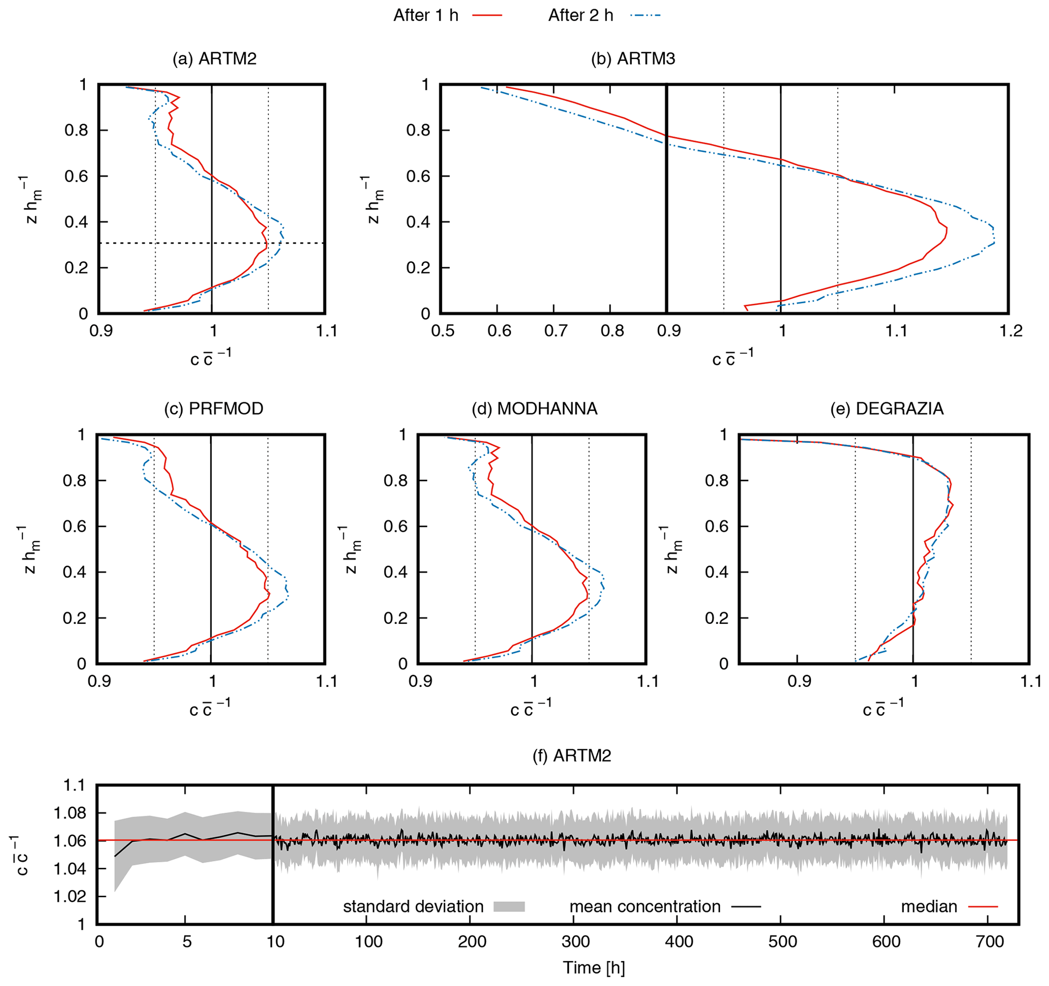
Figure 3Profiles of the concentration normalised to the mean concentration (a–e) of the different turbulence models, ARTM2, ARTM3, PRFMOD, MODHANNA, and DEGRAZIA, after 1 (red lines) and 2 h (dashed–dotted blue lines) for periodic lateral simulation domain boundaries and reflecting bottom and top boundaries. In (b) the x-axis scale changes at . (f) Time series of the normalised concentration at normalised height for the ARTM2 model, which is indicated by the dashed horizontal line in (a). The x-axis scale changes at 10 h.
The concentration profiles of the different turbulence models for very unstable PBL conditions are shown in Fig. 3. The concentrations of the state of mixing after 1 (red line) and 2 h (dashed blue line) are shown. Concentration values are normalised to the mean concentration (), and the height is normalised to the mixing depth (). We used the same initial numerical particle distribution for all turbulence models to eliminate possible differences arising from different initial distributions.
The concentration profiles after 1 h differ from the uniform distribution . This indicates a certain degree of segregation of the numerical particles, but most deviations are less than 5 % (vertical dashed lines). The largest deviations can be found at the top of the PBL for the ARTM3 model (> 35 %) and the DEGRAZIA model (> 15 %). The profiles of the ARTM2 and MODHANNA turbulence models are very similar since they both contain the same vertical turbulence parametrisation. The PRFMOD turbulence model differs slightly from the ARTM2 model due to modifications described in Eq. (11). The profile of ARTM3 shows trends of dilution and accumulation similar to ARTM2, PRFMOD, and MODHANNA but magnified in its extent. The profile of the DEGRAZIA turbulence model shows a different shape because of its different formulation of the turbulence parameters (see Eqs. 23, 24, and 26).
By t = 2 h, the dilution of the concentration has further increased at the bottom and top of the PBL, and the accumulation at (horizontal dashed black line) has further increased partly beyond 5 % but well below 10 % deviation for ARTM2, PRFMOD, MODHANNA, and DEGRAZIA. For ARTM3, the dilution at the ground almost vanishes, while the dilution above increases to 40 %, and the accumulation in the middle of the PBL increases to 18 %. After the second hour, no further changes are observed, as can be seen in Fig. 3f for the ARTM2 turbulence model at . Time series for other heights and other turbulence models show similar behaviour and are given in Sect. S2 in the Supplement.
This well-mixed condition test shows that the simulation result systematically overestimates the concentration values at for the ARTM2, PRFMOD, and MODHANNA models after the second hour. Near the surface, which is important for estimation of exposure to the population, the concentration values are underestimated. In both cases, the errors are only 5 %–6 %. At the top of the PBL, the models underestimate the expected concentration significantly. The ARTM3 turbulence model shows the smallest deviation from the mean domain concentration near the ground, but it overestimates the concentration in the middle of the PBL before substantially underestimating the mixing layer top. Below the DEGRAZIA turbulence model performs the best. At the top of the PBL the model decreases well below the expected concentration. All the tested turbulence models can be assumed to be acceptable for simulations in very unstable atmospheric conditions, but the partly large deviations of the concentration from the expected values at certain heights have to be taken into account when interpreting model results. Under low-wind conditions (1 m s−1 at 10 m height), the deviation from the uniform concentration is similar (see Sect. S2 in the Supplement).
The comparison of atmospheric dispersion simulation results with measurements near the ground is not sufficient to derive any conclusions about the three-dimensional structure of simulated emission plumes. To study the agreement of simulated and observed plume dispersion it is inevitable to use observations that resolve the structure of the real plume. Since ARTM simulates the emissions of nuclear facilities with source heights of mainly 100 to 200 m, it is useful to choose observational data originating from similar height levels. In this work, we present a comparison of ARTM simulations with airborne CO2 observations within the PBL. In such a case, the comparison is challenging because of the turbulent character of the PBL. As pointed out by Brunner et al. (2023), observations only provide snapshots of the real world, while simulations provide one realisation of a multitude of stochastic representations of the real world. Simulations with slightly perturbed initial conditions could result in different dispersion patterns of the plume. Furthermore, simulation results and observations may have different spatial and temporal resolutions and uncertainties, which complicates the comparison of simulations with observations (Farchi et al., 2016). Thus, in this work, the comparison of simulation results with observations for the five turbulence models is given using rather general plume characteristics, such as the plume width per transect and maximum mixing ratios.
5.1 Observational data
The aircraft observations used for this investigation originate from the Carbon Dioxide and Methane Mission (CoMet 1.0) (Fix et al., 2018; Luther et al., 2019; Fiehn et al., 2020; Gałkowski et al., 2021; Wolff et al., 2021; Krautwurst et al., 2021; Andersen et al., 2023; Brunner et al., 2023). The campaign took place in May and June 2018 and involved three aircraft performing in situ and remote sensing measurements. The objective was to study CO2 and methane (CH4) emissions from different sources in Europe, including power plants, and to compare the different observational methods.
For the evaluation of ARTM, airborne in situ CO2 measurements in the vicinity of the Bełchatów lignite power plant in Poland were used (Fiehn et al., 2020; Kostinek et al., 2021). An overview map with the CO2 mixing ratios along the flight path is shown in Fig. 4. The in situ measurements were performed on 7 June 2018 between 13:00 and 15:00 UTC aboard the DLR Cessna Grand Caravan 208B. One transect on the upwind side of the emitter was performed at the beginning in order to derive the mean background CO2 mixing ratio = 401.2 ppmv. The exhaust plume of the power plant was probed during several transects on the downwind side at heights between 500 and 1.7 They form two wall patterns at meridional distances of approx. 13 km (wall 1) and 23 km (wall 2) and a single transect at approx. 6 km from the source.
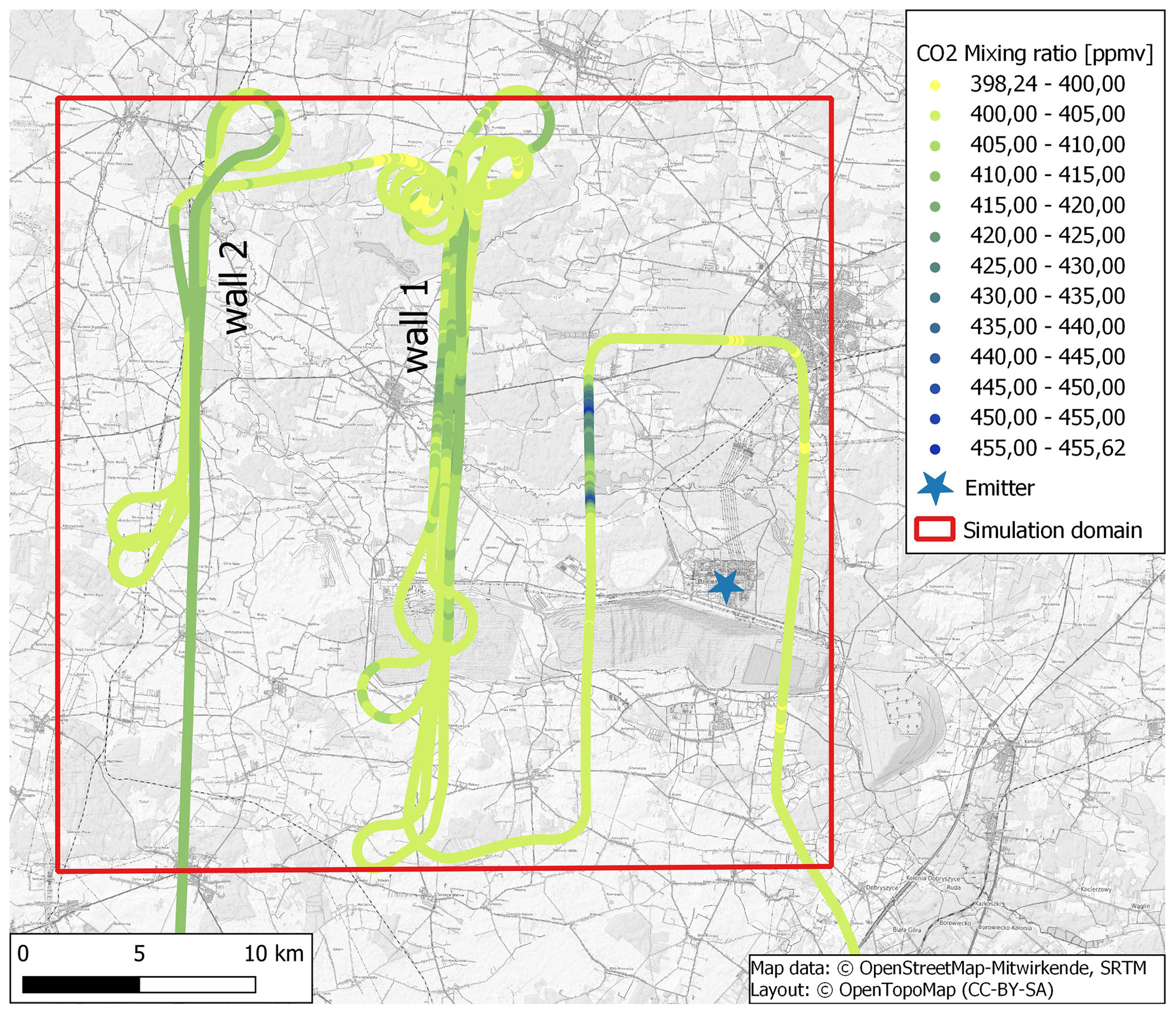
Figure 4Map showing the flight path of the DLR Cessna aircraft in the vicinity of the Bełchatów lignite power plant (blue star), colour-coded by the in-situ-measured CO2 values. Transects were performed both east (upwind side) and west (downwind side) of the emitting power plant. The red box indicates the simulation domain.
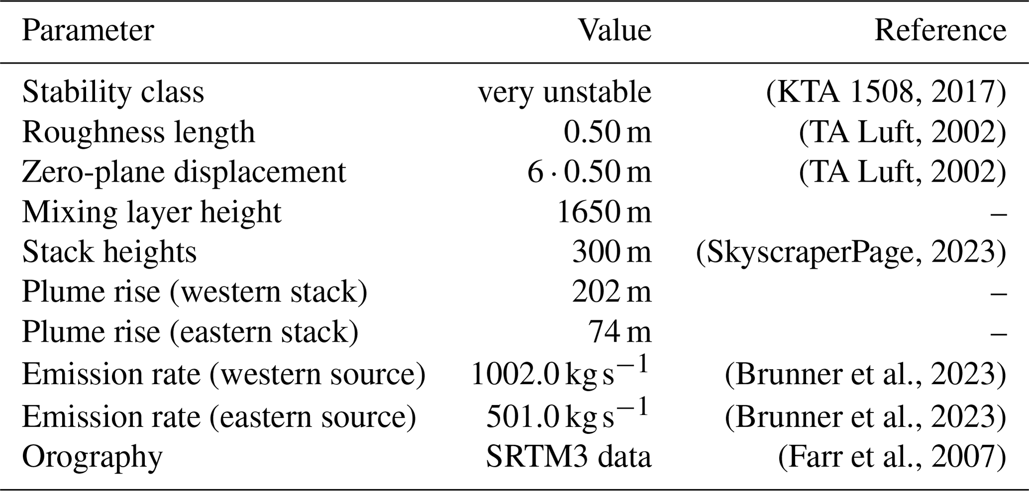
Table 4Input parameters needed by ARTM that are constant during the simulation run.
CO2 was measured with a cavity ring-down spectroscopy analyser (G1301-m, Picarro) specifically modified for the airborne deployment operating at 0.5 Hz. The CO2 measurement uncertainty is ± 0.15 ppmv, and the temporal resolution was increased to 1 s by interpolation to make the data comparable with other data collected during the campaign. Details of the measurement equipment and related uncertainties are described by Klausner et al. (2020). The sampling repetition and the velocity of the aircraft result in a spatial distance of about 140 m between the 0.5 Hz data points. The Picarro instrument measures CO2, methane, and water vapour sequentially, and thus the values are representative of the last third of the measurement interval. Observational data for wind direction, wind speed, and flight height are shown in Sect. S3 in the Supplement.
5.2 Model setup
We chose a simulation domain of 33.3 km × 33.3 km × 1.9 km that covers the horizontal extent of the flight trajectory and vertically extends beyond the mixing layer depth by four simulation levels. The horizontal resolution was 150 m. The extent of the simulation domain with the location of the emission source (two stacks over a distance of 300 m) is shown in Fig. 4. Vertically, the grid spacing gradually increases from 3 to 35 m until 100 m height is reached. Above, 50 m level thickness was used. All level thicknesses are given in Table S2 in the Supplement.
ARTM requires several input parameters: SC, z0, d0, orography, several source-specific parameters, and wind speed and direction at one location in the simulation domain. Since there were no stationary ground-based wind measurements available, wind direction, wind velocity, SC, and mixing layer height were derived from the airborne measurements. The actual emission rates are unknown. However, Brunner et al. (2023) estimated the overall CO2 emission rate according to the generated electrical power of the power plant, resulting in 1503.0 kg s−1 during the measurement flight. This corresponds to 123 % of the annual mean emission rate of 38.4 Mt CO2 reported by the power plant to the European Pollutant Release and Transfer Register (E-PRTR) for the year 2018. The description of the derivation of SC, z0, d0, and the plume rise as well as the orography data are given in Sect. S4 in the Supplement. The parameter values and the origin of the orography data are summarised in Table 4.
ARTM requires radionuclide emission rates in Bq s−1; thus we chose CO2 consisting of the radioactive isotope 14C for the simulations. Its decay constant λ=5730 ± 40 years leads to a decay of 5.5 × 10⁻⁶ %, which is negligible within the simulation period. Thus, ARTM's internal emission rates in Bq s−1 can be used as an equivalent for a mass rate in kg s−1 and to convert activity concentration into mixing ratio.
The wind speed (4.4 m s−1) and directions driving the simulation were derived from one flight transect (13:28:03 to 13:33:14 UTC) at a distance of ≈ 13 km to the west of the power plant at a height of ≈ 600 This transect is located close to the middle of the simulation domain and is therefore assumed to be representative. The histogram of the wind directions of the transect is shown in Fig. 5. Based on this histogram, two different setups of the model were selected:
- i.
A single wind direction of 120° (mean of the distribution) was selected, assuming that the wind fluctuations are part of the turbulence spectrum and should therefore be represented by the turbulence parametrisation of ARTM.
- ii.
Two different wind directions were used alternatingly to drive ARTM, a direction of 106° (mean of all directions < 120°) and a direction of 134° (mean of all directions > 120°). This assumes that part of the wind variation is due to mesoscale variability that cannot be resolved by ARTM's turbulence scheme.
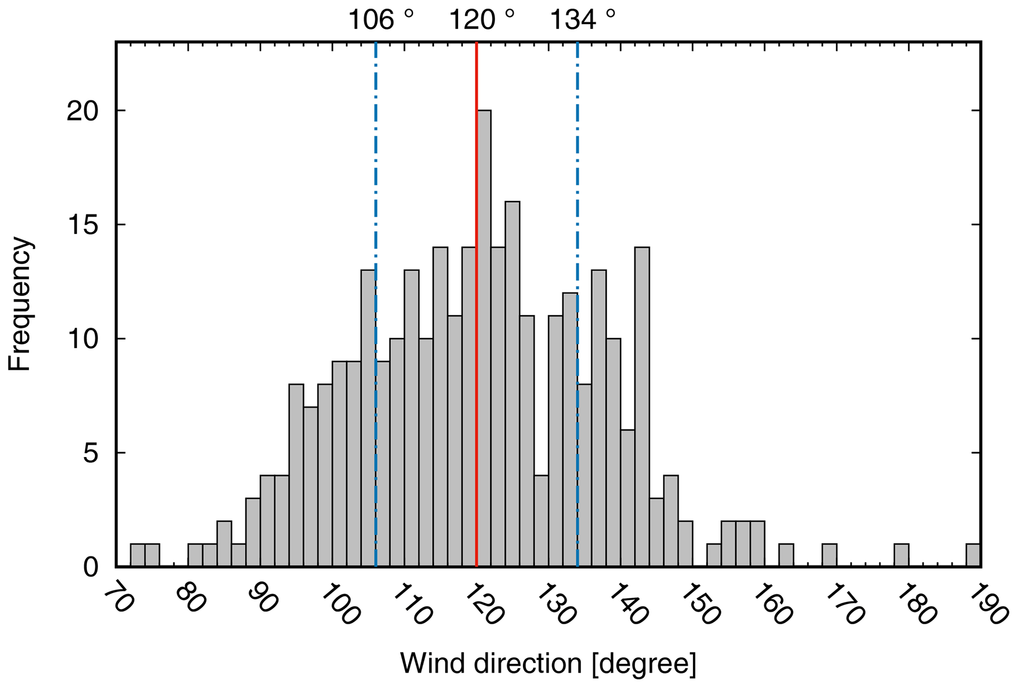
Figure 5Histogram of the wind directions of the transect chosen for the determination of the wind direction and wind velocity. The transect covers a duration from 13:28:03 to 13:33:14 UTC with the mean position 53.31° N, 19.15° E. The mean measurement height is 599 The mean value of the wind direction is 120° (red line). The mean value of the wind directions below 120° is 106° and above 120° is 134° (dashed blue lines).
The first setup was applied to all turbulence models, while the second setup was only tested for ARTM2. The hourly sequence of wind inputs for the model is summarised in Sect. S5 in the Supplement.
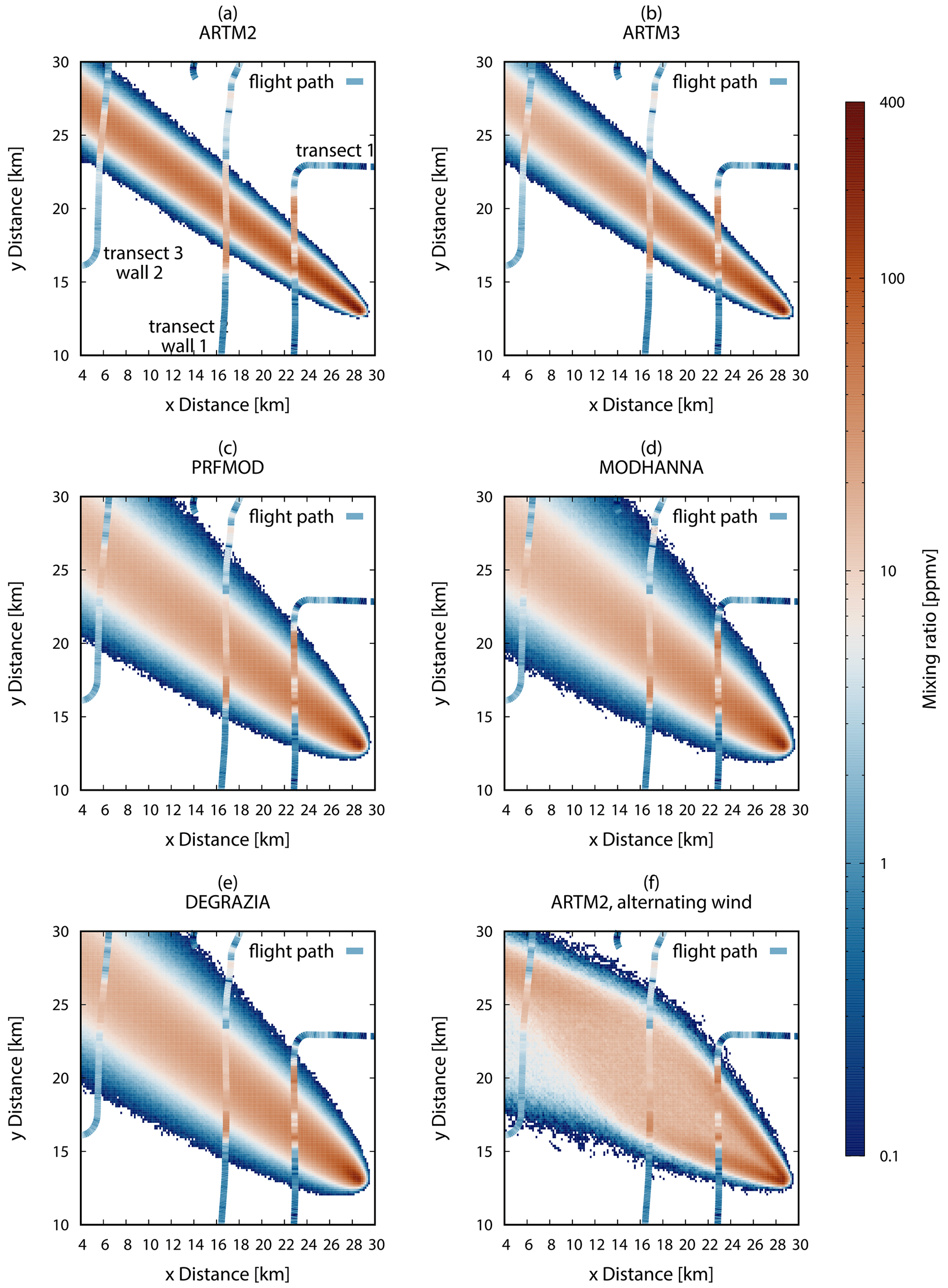
Figure 6Modelled CO2 mixing ratio for the case of one wind direction in (a) ARTM2, (b) ARTM3, (c) PRFMOD, (d) MODHANNA, and (e) DEGRAZIA and two wind directions in (f) ARTM2. The wind directions and speeds are given in Table S3 in the Supplement; the input parameters are given in Table 4. Mixing ratios of the simulated plume (averaged over the simulation time) at heights between 750 and 800 m and the in situ data along the flight path between 700 and 800 m are shown in logarithmic scale in ppmv. The case of two wind directions in (f) shows the mean CO2 mixing ratio of 2 subsequent hours for the duration of the measurement flight from 13:00 to 15:00 UTC. The background CO2 mixing ratio of 401 ppmv is subtracted from the observation.
5.3 Horizontal dispersion
The mixing ratio maps simulated with the five turbulence models at a height of 750 to 800 m are shown in Fig. 6 together with the observations between 700 and 800 m. We subtracted the background CO2 mixing ratio of 401 ppmv from the observations to make them comparable to the simulation results.
The simulated and observed mixing ratios of the plumes are of the same order of magnitude. The simulated plumes show the mean wind direction to be in agreement with the observed one; however, the meandering behaviour of the real plume can be observed at transects 1, 2, and 3 in Fig. 6, revealing that this behaviour is not covered by all turbulence models. The mixing ratio profile in the lateral (crosswind) direction simulated by ARTM resembles a Gaussian distribution. This is expected for a constant wind direction and wind speed (Thykier-Nielsen et al., 1999).
The different turbulence models clearly affect the simulated plume widths. The ARTM2 turbulence model simulates the narrowest plume. The ARTM3 model results in a slightly wider plume, but compared to the observations both are too narrow. The PRFMOD and DEGRAZIA turbulence models show much broader plumes that cover the observed one to a large extent. The widest plume is simulated by the MODHANNA turbulence model and is in good agreement with the observed plume width. The width of the plumes of the turbulence models is mainly attributed to the horizontal wind speed fluctuations and Lagrangian correlation times displayed in Fig. 2. The highest values for σy and TLy are simulated by MODHANNA, PRFMOD, and DEGRAZIA followed by ARTM3 and ARTM2 in the upper half of the PBL, in agreement with the simulated plume width.
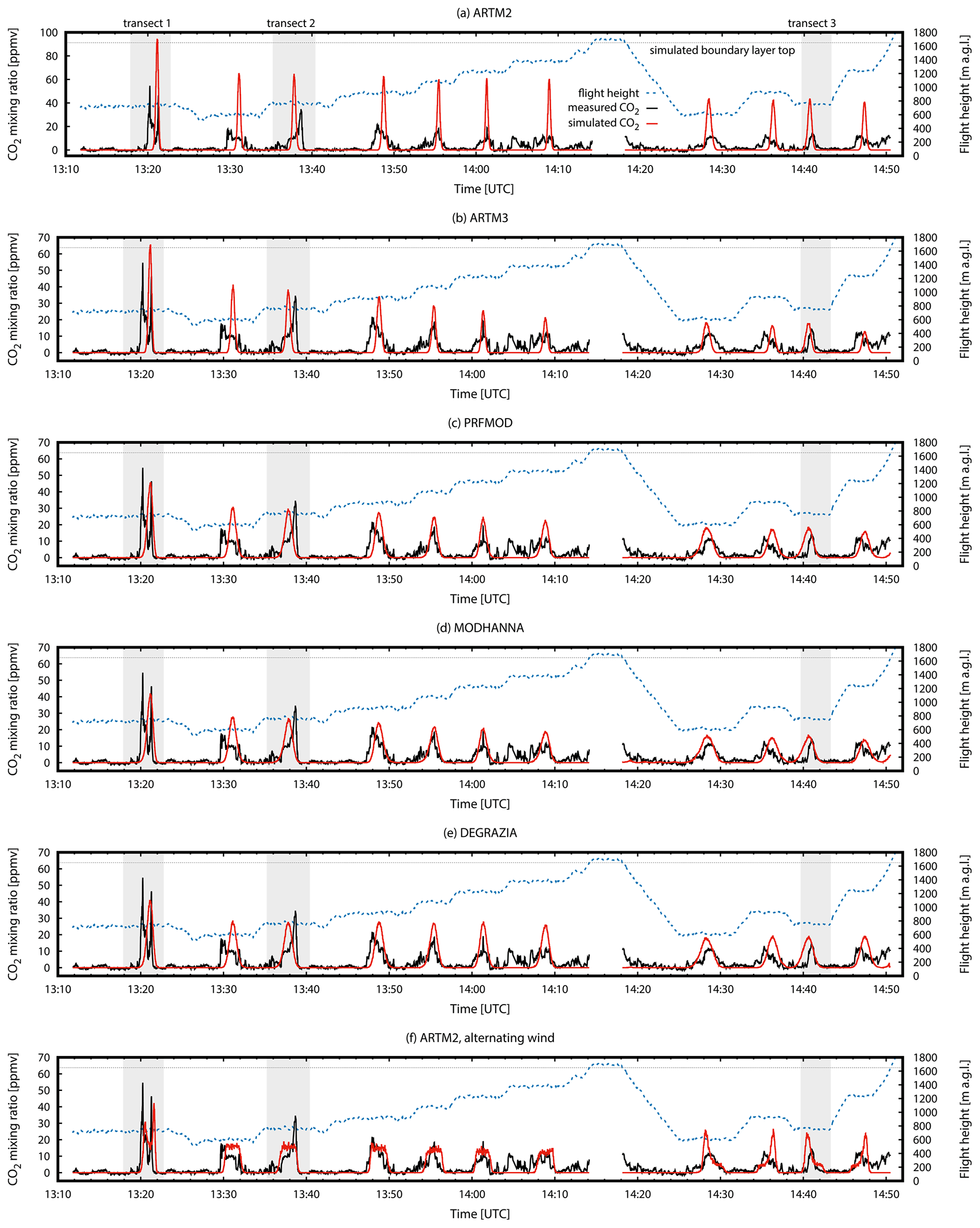
Figure 7Simulated (red line) and measured (black line) CO2 data along the flight path together with the flight height (dotted blue line) within the simulation domain. The (a) ARTM2, (b) ARTM3, (c) PRFMOD, (d) MODHANNA, and (e) DEGRAZIA turbulence models and the (f) ARTM2 turbulence model with two alternating wind directions. The transects shown in Fig. 6 are shaded in grey.
Figure 7 shows the simulated and observed plumes of the different turbulence models together with the flight height above ground level along the flight path. Transects 1, 2, and 3 are shaded in grey. Data above the simulated boundary layer top are excluded from the figures. In Fig. 7, the simulated maximum CO2 mixing ratios of ARTM2 are larger at all transects compared to the observations. Within the simulated boundary layer, this deviation reaches 300 % at 14:08 UTC and is attributed to the too-narrow simulated plume. With increasing plume width of the different turbulence models, the maximum mixing ratios decrease (see Fig. 7a–e). The ARTM3, PRFMOD, MODHANNA, and DEGRAZIA turbulence models simulate mixing ratio peaks similar to or below the observed values. Due to dispersion the mixing ratio maximums decrease with increasing distance from the source for all models, in agreement with the observation. It is important to point out that simulated mixing ratio values are highly dependent on the emission rates.
The simulation gives 1 h averages of the exhaust plume, which is expected as the mean of several realisations of meandering plumes. It is not expected that simulated values are much larger than the observed ones but can occur if the width of the simulated plume or the mixing layer depth are underestimated or the emission rate is overestimated.
An alternative to modelling the meandering behaviour via the turbulence is the usage of alternating wind directions for subsequent simulation hours for the ARTM2 turbulence model to explicitly simulate the meandering plume (Figs. 6f and 7f). Simulation results from subsequent hours are combined by calculating the average concentrations. The wind direction derivation is explained in Sect. 5.2. This method generates the widest plume covering the observations and mimics the structure of two maxima at transect 1. However, these two observed maxima originate from snapshots of the meandering plume and are not expected to be reproduced by the time-averaged simulation. Moreover, physically unrealistic plateaus of mixing ratios are simulated in wall 1 and a single narrow mixing ratio peak in wall 2, which is a result of the alternating wind directions. Mixing ratio maps of simulations and observations at other selected heights are given in Sect. S6 in the Supplement.
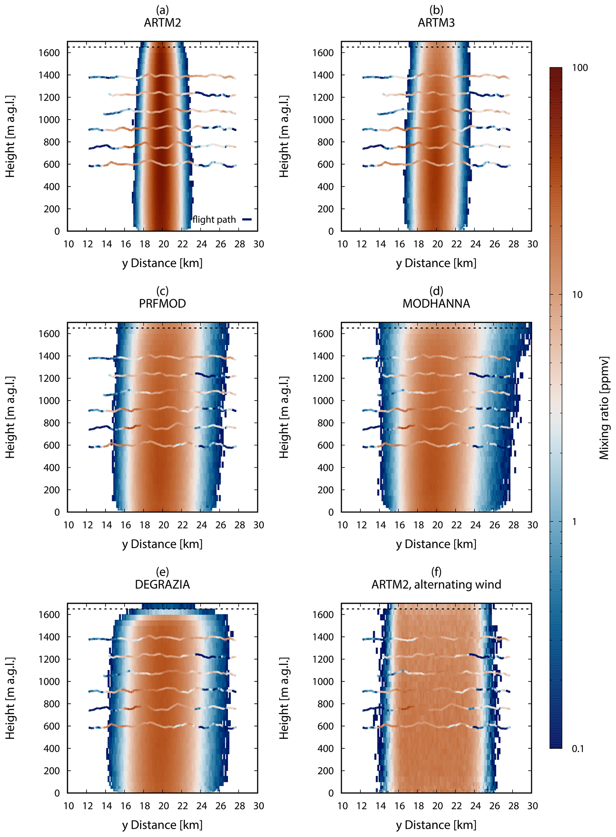
Figure 8Cross section of the simulated plumes at wall 1 of the observations for the different turbulence models: (a) ARTM2, (b) ARTM3, (c) PRFMOD, (d) MODHANNA, and (e) DEGRAZIA. (f) The case of two wind directions for ARTM2. The x-axis y distance is in a south–north orientation. The dashed line at 1650 marks the simulated mixing layer top.
5.4 Vertical dispersion
For the analysis of the vertical plume behaviour, the cross sections of the simulated plumes at wall 1 are presented in Fig. 8. The narrowest simulated plume is obtained by the ARTM2 model and underestimates the width of the observed plume at heights from 600 m to 1400 The plume of the ARTM3 model is slightly wider throughout the PBL. In both the ARTM3 and the PRFMOD model, the values of σy (TLy) decrease (increase) with height (see Fig. 2). While these opposing trends cancel each other out for the ARTM3 model, they lead to a slight increase in lateral dispersion with height for the PRFMOD model. The vertical profiles of σy and TLy of the MODHANNA model shown in Fig. 2c and d appear to lead to a slightly increasing dispersion, too. The DEGRAZIA model, in contrast, shows a constant behaviour for both σy and TLy. Below 200 m the widths of all five simulated plumes decrease towards the surface.
All turbulence models show a slight decrease in the mixing ratio with increasing height at a constant distance from the source (see Fig. 7), which agrees with observations. From the cross sections at wall 1 (Fig. 8), the average horizontal mixing ratio profiles are derived and shown in Fig 9. Except for the DEGRAZIA model, the decreasing mixing ratio with increasing height above 600 m can be recognised here as well. However, in Fig. 7 the highest maximum mixing ratios at wall 1 (13:25 to 14:10 UTC) occur at transect 2 for the measurements. The simulations, having the highest concentration values, instead show very similar peaks at the two lowest transects in wall 1.
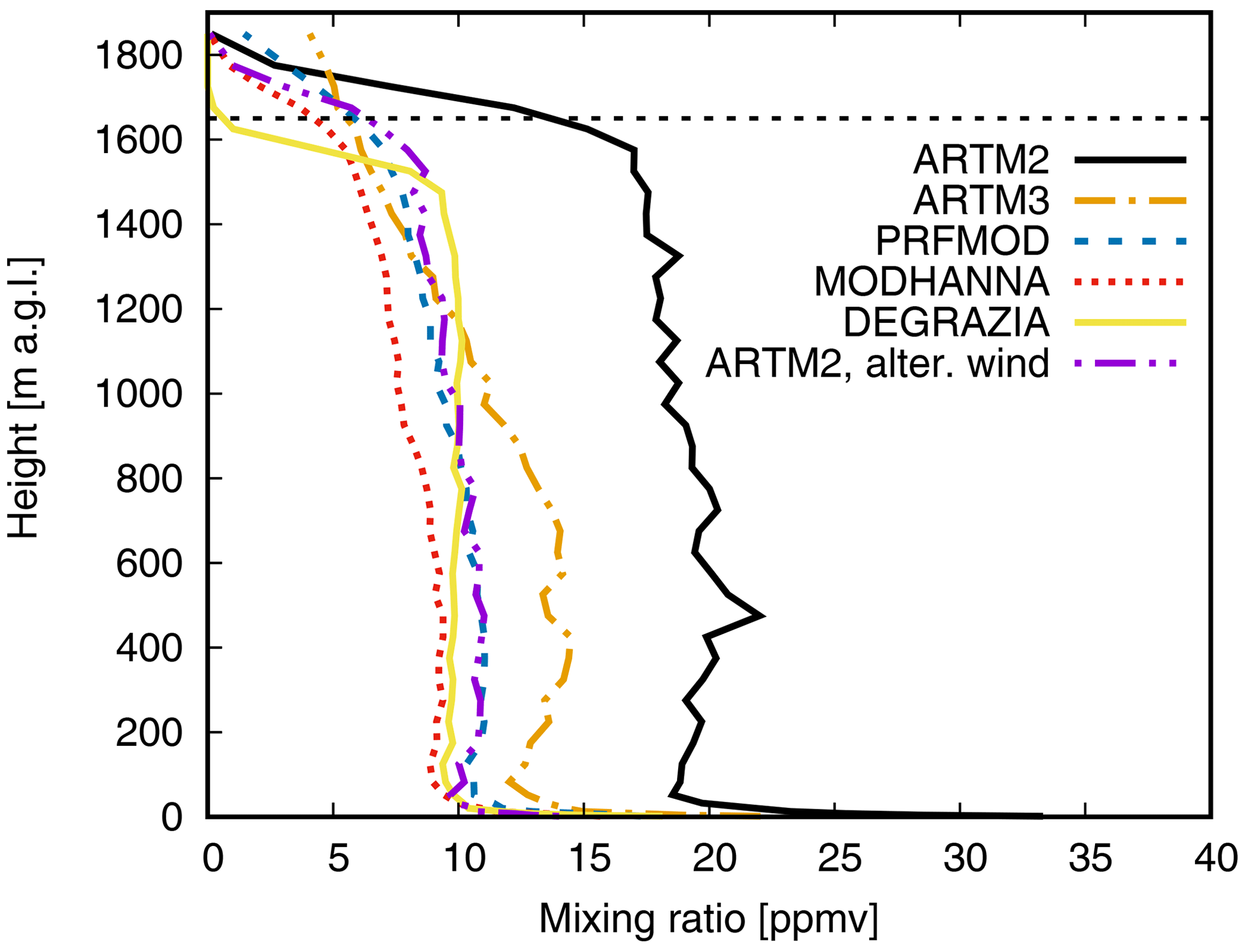
Figure 9Profile of the average horizontal mixing ratio of the six simulation cases at wall 1 (see Fig. 8). The dashed line at 1650 marks the simulated mixing layer top.
In contrast to the Gaussian lateral mixing ratio distribution of the plume in Fig. 8a, the ARTM2 turbulence model with two alternating wind directions (Fig. 8f) shows the uniform mixing ratio distribution in the plume's core region (mixing ratio > 1 ppmv), as shown in Fig. 7f.
The cross sections of wall 2 in Fig. S12 in the Supplement show a similar behaviour of the plumes. The measured data show a large variation in the plume width on the different transects, emphasising the meandering and turbulent character of the real plume. Furthermore, it can be recognised that the real plume is not entirely recorded; the transects are too short at this wall.
5.5 Validation and uncertainty evaluation
In order to quantify the simulations' uncertainty, we investigate the deviations of the simulated and the observed CO2 mixing ratios in the plume through probability distributions (PDs), comparisons of integrated plume mass, and point-to-point mixing ratio comparisons.
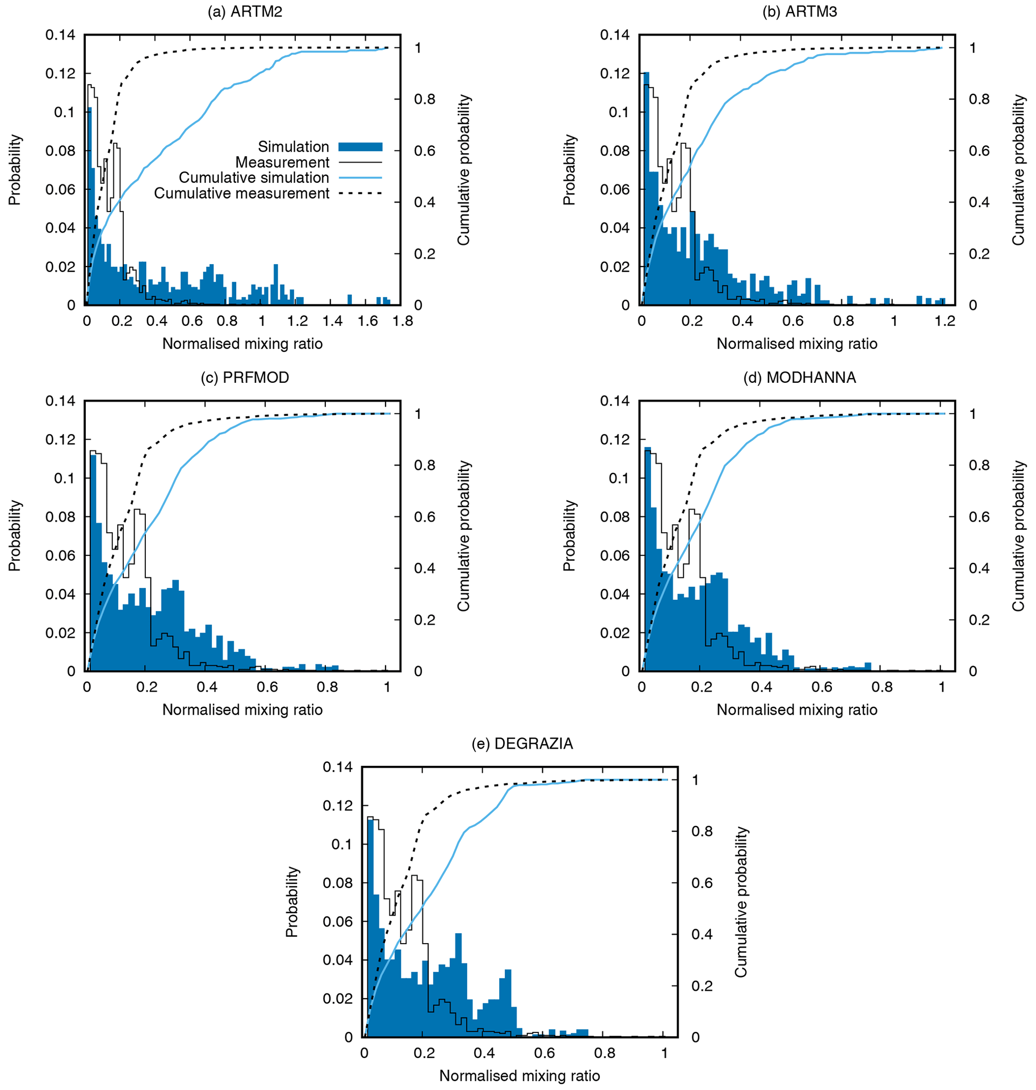
Figure 10Probability distribution (bars) and cumulative probability distribution (lines) of the simulated and measured mixing ratios of the five turbulence models. The PDs are normalised according to the maximum mixing ratio of the measurements, and the integral of the simulated and measured PDs is equal. Mixing ratio values below 1 ppmv are not considered in the PDs and CPDs.
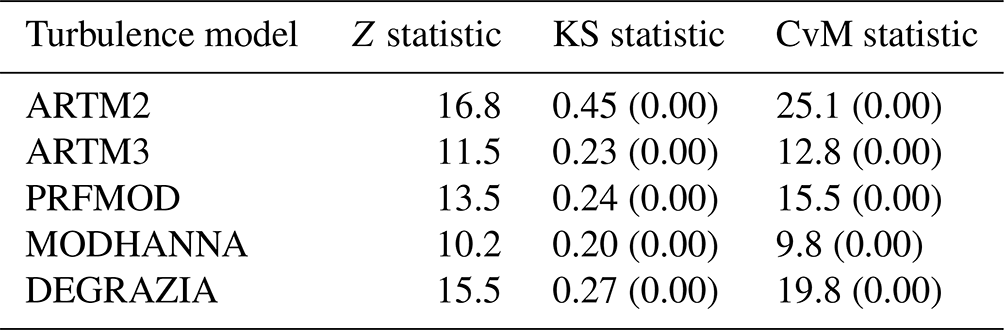
The deviation of model results and measurements in a plume can be accessed by the comparison of the PDs and the cumulative probability distributions (CPDs) of simulated and observed CO2 mixing ratios in the plume. The PDs of the simulation and measurement are normalised to the maximum mixing ratio of the measurements with the integrals of the simulated and measured distributions being equal. To get rid of the mixing ratio fluctuation in the excess mixing ratio of the measurement, mixing ratio values below 1 ppmv are not taken into account. The PDs and CPDs of the five different turbulence models and the observations for all transects below the simulated boundary layer top are given in Fig. 10. The PDs of the simulated and measured plume show the occurrence of mixing ratio values relative to the maximum mixing ratio of the measurements. There is an overestimation of the simulated maximum mixing ratios for the ARTM2 and ARTM3 turbulence models. The high number of data points at approx. 20 % of the maximum mixing ratio of the measurements is due to the fine structure, shoulders beside peaks, and broad indistinct peaks of the plume not represented in the simulations. MODHANNA can be identified as the turbulence model that shows the best agreement with the observations concerning the PDs and CPDs; i.e. the occurrence of the mixing ratio values is the most similar to that of the measurement. To quantify the similarity and to decide whether simulations and measurements are significantly different, three statistical test were applied: the Z test, the Kolmogorov–Smirnov (KS) test, and the Cramér–von Mises (CvM) test (Conover, 1980; Wilks, 2006; University of Oregon, 2020). The Z statistic represents the distance between the means of two PDs normalised to the standard error. Statistics below 2 indicate no significant difference between the distributions. Additional interpretation limits are given in Sect. S7 in the Supplement. The KS statistic represents the supremum of the distance between two CPDs, while the CvM statistic is proportional to the integral of the distances between two CPDs. For both we assumed a significance level of 0.05. The statistics and their p values (in brackets) are summarised in Table 5. The three statistical tests show that all simulated mixing ratio distributions differ significantly from the observed one. Nevertheless, the statistics can be used to rank the models. MODHANNA shows the best agreement with the observations; i.e. the distribution of mixing ratio values in the transects is the most similar to that of the observations compared to the other turbulence models. The statistical tests rank ARTM3 second, but this may be biased by the statistical tests being very sensitive to deviations in the regions of the PDs with high numbers of low mixing ratio values. We want to point out that the results do not mean that the MODHANNA model produces mixing ratio peaks that are structured like the observed ones, but the relative occurrence of mixing ratio values is the most similar.
Table 5Z statistics, Kolmogorov–Smirnov (KS) statistics, and Cramér–von Mises (CvM) statistics of the mixing ratio distributions of the five turbulence models. The p values are given in brackets. The significance level is 0.05.
To compare the simulation results, the integral of the mixing ratio values along the flight path below the simulated boundary layer top (see Fig. 7) within the plume is shown in Table 6. We used the method above to get rid of the baseline fluctuations in the excess mixing ratios to calculate the integrals. This procedure is also applied to the simulations. Except for ARTM3, there is good agreement between the modelled and measured data: the deviation is less than 13 %. Concerning ARTM3, there is a strong vertical gradient in the simulated mixing ratios of the plume above 700 m, as is illustrated in Figs. 8b and 9. Tracers are more strongly diluted (accumulated) in the upper (lower) half of the PBL than in the other turbulence models. This corresponds to the findings presented in Sect. 4. Since the flight path is mainly located in the upper half of the PBL, the integral along the flight path results in a lower value for ARTM3. The higher mixing ratios in the lower half of the PBL might become important when simulations are used for radiation exposure assessment. The results suggest that the original assumption of the emission rate may not deviate much from the actual value. However, observations below 600 m are necessary to get a more complete comparison of the simulated and actual plumes.
Table 6Integrals of mixing ratio values (values below 1 ppmv are not considered) along the flight path for simulation Asim and observation Aobs within the simulated PBL (see Fig. 7) given in ppmv km and their ratio.
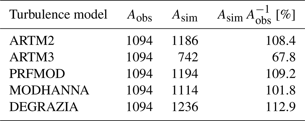
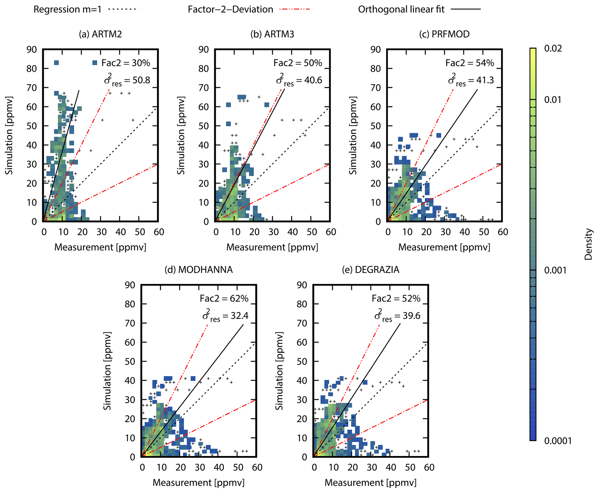
Figure 11Density scatterplots of the simulated mixing ratios of the five turbulence models, ARTM2 (a), ARTM3 (b), PRFMOD (c), MODHANNA (d), and DEGRAZIA (e), against the observations. Single data points in a bin are indicated with +; more data points in a bin are colour-coded. The regression with slope m=1 (dotted black line) represents the identification of the simulation with the measurement, the dotted–dashed red line represents a deviation from the regression with m=1 by a factor of 2, and the solid black line represents the orthogonal linear fit to the data points. Fac2 gives the percentage of data points with deviations of not more than a factor of 2 from the regression m=1. The residual variance of the orthogonal fit is given by .
The deviation between the simulations of the five turbulence models and the observation at a specific position can be assessed using density scatterplots as given in Fig. 11. All mixing ratio values larger than 1 ppm along the flight path below the simulated boundary layer top are considered. The regression with slope m=1 is shown with a dashed line and represents the equality of the simulated and observed mixing ratios. The deviation from this equality by a factor of 2 is confined by the dashed–dotted red lines. It is not expected to find a lot of data points at the regression m=1 due to the fundamental differences in the data set properties of the simulation and observation. However, a large number of data points within a deviation of a factor of 2 decreases the uncertainty. The percentage of data points within these borders is represented as Fac2 (Fig. 11). Low Fac2 values can also be explained by the large number of measurement data points outside the simulated plume because they are too narrow. The smallest Fac2 is derived for the ARTM2 model. This coincides with the unbalanced distribution of the data points around the regression m=1, with the simulation overestimating the observed mixing ratios and simultaneously simulating too-narrow plumes. This is represented by the orthogonal regression of data points (black line) given in the figure with a slope above 3. The residual variance quantifies the scattering of data points. The large value for ARTM2 indicates a less compact data point distribution. ARTM3 shows more balanced and compact data but still distinctly overestimates mixing ratios and underestimates plume widths. PRFMOD, MODHANNA, and DEGRAZIA show similar properties with Fac2 > 50 %; more compact, well-balanced data; and less overestimated mixing ratios and underestimated plume widths, with the MODHANNA model performing slightly better for the given measurement and turbulence conditions.
The uncertainty in the CO2 measurement device of ± 0.15 ppmv is at least 1 order of magnitude smaller than the measured enhanced CO2 concentrations. Thus, the measurement uncertainty has only a minor impact on the evaluation results.
In this work we present an extensive evaluation of ARTM with three different elements: a sensitivity analysis, an analysis of turbulence models, and a comparison with aircraft observations. Based on the sensitivity analysis, we identified the stability class to be the most important input parameter, followed by the roughness length, the source height, and the displacement height factor. Therefore, special care has to be taken to determine the stability class for a simulation because uncertainties in this parameter cause large uncertainties in model results. This emphasises the general disadvantage of the rather coarse stability class concept being used to describe atmospheric turbulence. A finer classification or a continuous parameter such as the Obukhov length could be a better option but would generally require detailed measurements of turbulence parameters such as friction velocity and sensible heat flux.
In addition to the three turbulence models already implemented in ARTM 3.0.0, two other turbulence models, the MODHANNA model and the DEGRAZIA model, were implemented and tested. Evaluation of the models by applying the well-mixed condition test showed that the ARTM2, PRFMOD, and MODHANNA models produced a moderate deviation of an initially uniform concentration profile under unstable atmospheric boundary layer conditions. Underestimations of the uniform concentration occur primarily at the ground and at the top of the boundary layer with up to 10 %, while overestimations occur in between with up to 7 % at one-third of the PBL. Under the same conditions the ARTM3 model produces the strongest deviations: up to 4 times higher than the other models. However, near the ground ARTM3 performs the best. The DEGRAZIA model showed a less inhomogeneous profile with deviations from the uniform concentration of 5 % or less below z=0.8hm. The discrepancies under 6 % below 80 % of the boundary layer height show good mixing properties of the unstable planetary boundary layer for the ARTM2, PRFMOD, MODHANNA, and DEGRAZIA models.
Three-dimensional airborne in situ observational data measuring a power plant emission plume were compared to ARTM simulation results. The time resolution of ARTM results is 1 h, which is larger than the expected timescale of the observed meandering plume, and, therefore, ARTM is expected to capture the time-integrated real plume and not the fine structures on small scales. ARTM simulated the mean wind in agreement with the observations throughout the simulation domain. The different turbulence models simulate plume mixing ratios of the same order of magnitude as the measurements, although the exact mixing ratio values depend on the emission rate. ARTM2 underestimates the plume spread under very unstable conditions and overestimates the maximum mixing ratio by a factor of 2 or more. The ARTM3 model produces only slightly wider plumes in the lateral direction but lower maximum mixing ratio values at the upper half of the PBL. This is attributed to the inhomogeneous vertical mixing and the horizontal turbulence parametrisation of the ARTM3 turbulence model under unstable conditions. The other turbulence models, PRFMOD, MODHANNA, and DEGRAZIA, simulate a wider plume spread in the range of the measurements. Maximum mixing ratios are close to the measurements, and the integrals of the mixing ratios of the simulations and observations along the flight path are comparable. The models were evaluated with measurements at heights larger than 600 m and hence do not cover the heights below 600 m. The differences in the temporal and local resolutions of the simulations and measurements lead to differences in the distributions of mixing ratio values. According to Fig. 10, under unstable conditions, all turbulence models underestimate the occurrence of mixing ratio values by around 20 % of the maximum mixing ratio of the measurements, which is a result of the fine structure of the plumes. The smallest deviations in PDs and CPDs are found for MODHANNA. Using point-to-point comparisons, the ARTM2 model showed the largest deviations from the measured plume; ARTM3 showed better agreement; and PRFMOD, MODHANNA, and DEGRAZIA showed comparable good performances, with MODHANNA matching the measurements slightly better than the others.
With the results of this study we showed that ARTM is able to simulate the extension and mixing ratios of a plume under unstable stratification conditions when the proper turbulence model is used. The ARTM3 model was shown to be a suitable turbulence model for radiation exposure assessment when conservative long-term simulations are requested. However, the PRFMOD, MODHANNA, and DEGRAZIA models simulate the exhaust plume closer to real exhaust plumes under the given conditions and under the limitations of temporal and spatial uncertainties. Within this validation using the in situ data from the Bełchatów power plant, the MODHANNA turbulence model performed slightly better. However, this ranking cannot be generalised to other stability conditions without further comparison studies. Further analyses with known emission terms with different atmospheric turbulence properties, stable and neutral conditions, are necessary and can lead to better validation of ARTM. We encourage the comparison of other turbulence formulations, such as the one suggested by Hanna (1982). This would also reveal differences between the model of Hanna (1982) and the DEGRAZIA model and extends the analyses given by Carvalho et al. (2002) to larger heights. The collection of measurement data in the upper and lower half of the PBL and transects sampling the entire extent of a plume are beneficial. Moreover, the use of the Obukhov length as a measure of atmospheric stability is encouraged.
The ARTM programme is available upon request to the Federal Office for Radiation Protection (BfS) of Germany via artm@bfs.de. The data from the CoMeT 1.0 campaign are available at https://halo-db.pa.op.dlr.de/mission/94 (last access: 21 January 2024).
The supplement related to this article is available online at: https://doi.org/10.5194/acp-24-2511-2024-supplement.
Conceptualisation: RH, MPÁ, DB, CV; data collection: AF, AR; methodology: RH, MPÁ, DB, CV; formal analysis: RH; writing (original draft preparation): RH; writing (review and editing): MPÁ, RH, DB, CV, AF, AR; supervision: MPÁ, DB, CV.
The contact author has declared that none of the authors has any competing interests.
Publisher's note: Copernicus Publications remains neutral with regard to jurisdictional claims made in the text, published maps, institutional affiliations, or any other geographical representation in this paper. While Copernicus Publications makes every effort to include appropriate place names, the final responsibility lies with the authors.
This article is part of the special issue “CoMet: a mission to improve our understanding and to better quantify the carbon dioxide and methane cycles”. It is not associated with a conference.
We thank Christopher Strobl (BfS) for his support. Furthermore, we would like to thank Stephan Henne (Empa) for helpful discussions.
BfS funded the PhD position that resulted in this work.
This paper was edited by Christoph Gerbig and reviewed by two anonymous referees.
Andersen, T., Zhao, Z., de Vries, M., Necki, J., Swolkien, J., Menoud, M., Röckmann, T., Roiger, A., Fix, A., Peters, W., and Chen, H.: Local-to-regional methane emissions from the Upper Silesian Coal Basin (USCB) quantified using UAV-based atmospheric measurements, Atmos. Chem. Phys., 23, 5191–5216, https://doi.org/10.5194/acp-23-5191-2023, 2023. a
Arnold, D., Maurer, C., Wotawa, G., Draxler, R., Saito, K., and Seibert, P.: Influence of the meteorological input on the atmospheric transport modelling with FLEXPART of radionuclides from the Fukushima Daiichi nuclear accident, J. Environ. Radioactiv., 139, 212–225, https://doi.org/10.1016/j.jenvrad.2014.02.013, 2015. a
Bahlali, M. L., Henry, C., and Carissimo, B.: On the Well-Mixed Condition and Consistency Issues in Hybrid Eulerian/Lagrangian Stochastic Models of Dispersion, Bound.-Lay. Meteorol., 174, 275–296, https://doi.org/10.1007/s10546-019-00486-9, 2020. a
Berchet, A., Zink, K., Oettl, D., Brunner, J., Emmenegger, L., and Brunner, D.: Evaluation of high-resolution GRAMM–GRAL (v15.12/v14.8) NOx simulations over the city of Zürich, Switzerland, Geosci. Model Dev., 10, 3441–3459, https://doi.org/10.5194/gmd-10-3441-2017, 2017. a
Borgonovo, E.: A new uncertainty importance measure, Reliab. Eng. Syst. Safe., 92, 771–784, https://doi.org/10.1016/j.ress.2006.04.015, 2007. a, b, c
Brunner, D., Kuhlmann, G., Henne, S., Koene, E., Kern, B., Wolff, S., Voigt, C., Jöckel, P., Kiemle, C., Roiger, A., Fiehn, A., Krautwurst, S., Gerilowski, K., Bovensmann, H., Borchardt, J., Galkowski, M., Gerbig, C., Marshall, J., Klonecki, A., Prunet, P., Hanfland, R., Pattantyús-Ábrahám, M., Wyszogrodzki, A., and Fix, A.: Evaluation of simulated CO2 power plant plumes from six high-resolution atmospheric transport models, Atmos. Chem. Phys., 23, 2699–2728, https://doi.org/10.5194/acp-23-2699-2023, 2023. a, b, c, d, e, f, g, h
Carvalho, J. C., Anfossi, D., Trini Castelli, S., and Degrazia, G. A.: Application of a model system for the study of transport and diffusion in complex terrain to the TRACT experiment, Atmos. Environ., 36, 1147–1161, https://doi.org/10.1016/S1352-2310(01)00559-3, 2002. a
Chino, M., Nakayama, H., Nagai, H., Terada, H., Katata, G., and Yamazawa, H.: Preliminary Estimation of Release Amounts of 131I and 137Cs Accidentally Discharged from the Fukushima Daiichi Nuclear Power Plant into the Atmosphere, J. Nucl. Sci. Technol., 48, 1129–1134, https://doi.org/10.1080/18811248.2011.9711799, 2011. a
Connan, O., Smith, K., Organo, C., Solier, L., Maro, D., and Hébert, D.: Comparison of RIMPUFF, HYSPLIT, ADMS atmospheric dispersion model outputs, using emergency response procedures, with 85Kr measurements made in the vicinity of nuclear reprocessing plant, J. Environ. Radioactiv., 124, 266–277, https://doi.org/10.1016/j.jenvrad.2013.06.004, 2013. a
Conover, W. J.: Practical Nonparametric Statistics, 2 edn., Wiley & Sons, New York, ISBN 0-471-02867-3, 1980. a
Cox, R. M., Sontowski, J., and Dougherty, C. M.: An evaluation of three diagnostic wind models (CALMET, MCSCIPUF, and SWIFT) with wind data from the Dipole Pride 26 field experiments, Meteorol. Appl., 12, 329–341, https://doi.org/10.1017/S1350482705001908, 2005. a
Degrazia, G. A., Anfossi, D., Carvalho, J. C., Mangia, C., Tirabassi, T., and Campos Velho, H. F.: Turbulence parameterisation for PBL dispersion models in all stability conditions, Atmos. Environ., 34, 3575–3583, https://doi.org/10.1016/S1352-2310(00)00116-3, 2000. a, b, c
Draxler, R., Arnold, D., Chino, M., Galmarini, S., Hort, M., Jones, A., Leadbetter, S., Malo, A., Maurer, C., Rolph, G., Saito, K., Servranckx, R., Shimbori, T., Solazzo, E., and Wotawa, G.: World Meteorological Organization's model simulations of the radionuclide dispersion and deposition from the Fukushima Daiichi nuclear power plant accident, J. Environ. Radioactiv., 139, 172–184, https://doi.org/10.1016/j.jenvrad.2013.09.014, 2015. a
Draxler, R. R. and Hess, G. D.: An overview of the HYSPLIT_4 modelling system for trajectories, dispersion and deposition, Aust. Meteorol. Mag., 47, 295–308, 1998. a
Farchi, A., Bocquet, M., Roustan, Y., Mathieu, A., and Quérel, A.: Using the Wasserstein distance to compare fields of pollutants: application to the radionuclide atmospheric dispersion of the Fukushima-Daiichi accident, Tellus B, 68, 31682, https://doi.org/10.3402/tellusb.v68.31682, 2016. a
Farr, T. G., Rosen, P. A., Caro, E., Crippen, R., Duren, R., Hensley, S., Kobrick, M., Paller, M., Rodriguez, E., Roth, L., Seal, D., Shaffer, S., Shimada, J., Umland, J., Werner, M., Oskin, M., Burbank, D., and Alsdorf, D.: The Shuttle Radar Topography Mission, Rev. Geophys., 45, RG2004, https://doi.org/10.1029/2005RG000183, 2007. a
Fiehn, A., Kostinek, J., Eckl, M., Klausner, T., Gałkowski, M., Chen, J., Gerbig, C., Röckmann, T., Maazallahi, H., Schmidt, M., Korbeń, P., Neçki, J., Jagoda, P., Wildmann, N., Mallaun, C., Bun, R., Nickl, A.-L., Jöckel, P., Fix, A., and Roiger, A.: Estimating CH4, CO2 and CO emissions from coal mining and industrial activities in the Upper Silesian Coal Basin using an aircraft-based mass balance approach, Atmos. Chem. Phys., 20, 12675–12695, https://doi.org/10.5194/acp-20-12675-2020, 2020. a, b
Fix, A., Amediek, A., Bovensmann, H., Ehret, G., Gerbig, C., Gerilowski, K., Pfeilsticker, K., Roiger, A., and Zöger, M.: CoMet: An Airborne Mission to Simultaneously Measure CO2 and CH4 Using Lidar, Passive Remote Sensing, and In-Situ Techniques, EPJ Web Conf., 176, 02003, https://doi.org/10.1051/epjconf/201817602003, 2018. a, b
Frey, H. C. and Patil, S. R.: Identification and Review of Sensitivity Analysis Methods, Risk Anal., 22, 553–578, https://doi.org/10.1111/0272-4332.00039, 2002. a
Gałkowski, M., Jordan, A., Rothe, M., Marshall, J., Koch, F.-T., Chen, J., Agusti-Panareda, A., Fix, A., and Gerbig, C.: In situ observations of greenhouse gases over Europe during the CoMet 1.0 campaign aboard the HALO aircraft, Atmos. Meas. Tech., 14, 1525–1544, https://doi.org/10.5194/amt-14-1525-2021, 2021. a
Gariazzo, C., Papaleo, V., Pelliccioni, A., Calori, G., Radice, P., and Tinarelli, G.: Application of a Lagrangian particle model to assess the impact of harbour, industrial and urban activities on air quality in the Taranto area, Italy, Atmos. Environ., 41, 6432–6444, https://doi.org/10.1016/j.atmosenv.2007.06.005, 2007. a
Gesellschaft für Anlagen- und Reaktorsicherheit: ARTM Atmospheric Radionuclide-Transport-Model (version 2.8.0), Source Code, distributed by Federal Office for Radiation Protection of Germany upon request via artm@bfs.de, 2015. a
Gryning, S. E., Holtslag, A. A. M., Irwin, J. S., and Sivertsen, B.: Applied Dispersion Modelling Based on Meteorological Scaling Parameters, Atmos. Environ. (1967), 21, 79–89, https://doi.org/10.1016/0004-6981(87)90273-3, 1987. a
Hamby, D. M.: A Review of Techniques for Parameter Sensitivity Analysis of Environmental Models, Environ. Monit. Assess., 32, 135–154, https://doi.org/10.1007/BF00547132, 1994. a, b
Hamby, D. M.: A Comparison of Sensitivity Analysis Techniques, Health Phys., 68, 195–204, https://journals.lww.com/health-physics/Fulltext/1995/02000/A_Comparison_of_Sensitivity_Analysis_Techniques.5.aspx (last access: 21 January 2024), 1995. a
Hanfland, R., Pattantyús-Ábrahám, M., Richter, C., Brunner, D., and Voigt, C.: The Lagrangian Atmospheric Radionuclide Transport Model (ARTM) – development, description and sensitivity analysis, Air Qual. Atmos. Hlth., https://doi.org/10.1007/s11869-022-01188-x, 2022. a, b, c, d, e, f, g, h, i
Hanna, S. R.: Applications in Air Pollution Modeling, Springer Netherlands, Dordrecht, https://doi.org/10.1007/978-94-010-9112-1_7, pp. 275–310, 1982. a, b, c, d, e
Herman, J. and Usher, W.: SALib: An open-source Python library for Sensitivity Analysis, Journal of Open Source Software, 2, 97, https://doi.org/10.21105/joss.00097, 2017. a, b
Herman, J. and Usher, W.: SALib: Basics, https://salib.readthedocs.io/en/latest/user_guide/basics.html (last access: 11 April 2022), 2021. a, b
Hettrich, S.: Validation and Verification of the Atmospheric Radionuclide Transport Model (ARTM), Thesis, https://doi.org/10.5282/edoc.20914, 2017. a, b
Hicks, B. B.: Behavior of Turbulence Statistics in the Convective Boundary Layer, J. Appl. Meteorol. Clim., 24, 607–614, https://doi.org/10.1175/1520-0450(1985)024<0607:BOTSIT>2.0.CO;2, 1985. a
Hoffman, F. O. and Gardner, R. H.: Evaluation of Uncertainties in Environmental Radiological Assessment Models, book section 11, U. S. Nuclear Regulatory Commission, Washington, https://www.nrc.gov/docs/ML0917/ML091770419.pdf (last access: 21 January 2024), 1983. a
Iman, R. L. and Helton, J. C.: An Investigation of Uncertainty and Sensitivity Analysis Techniques for Computer Models, Risk Anal., 8, 71–90, https://doi.org/10.1111/j.1539-6924.1988.tb01155.x, 1988. a
Janicke, U. and Janicke, L.: Some aspects of the definition of meteorological boundary layer profiles and comparisons with measurements, Report, Janicke Consulting, https://www.janicke.de/data/bzu/bzu-007-01.pdf (last access: 21 January 2024), 2011. a, b
Joe, S. and Kuo, F. Y.: Constructing Sobol' Sequences with Better Two-Dimensional Projections, SIAM J. Sci. Comput., 30, 2635–2654, https://doi.org/10.1137/070709359, 2008. a
Katharopoulos, I., Brunner, D., Emmenegger, L., Leuenberger, M., and Henne, S.: Lagrangian Particle Dispersion Models in the Grey-Zone of Turbulence: Adaptions to FLEXPART-COSMO for Simulations at 1 km Grid Resolution, Bound.-Lay. Meteorol., 185, 129–160, https://doi.org/10.1007/s10546-022-00728-3, 2022. a
Kerschgens, M. J., Nölle, C., and Martens, R.: Comments on turbulence parameters for the calculation of dispersion in the atmospheric boundary layer, Meteorol. Z., 9, 155–163, https://doi.org/10.1127/metz/9/2000/155, 2000. a
Klausner, T., Mertens, M., Huntrieser, H., Gałkowski, M., Kuhlmann, G., Baumann, R., Fiehn, A., Jöckel, P., Pühl, M., and Roiger, A.: Urban greenhouse gas emissions from the Berlin area: A case study using airborne CO2 and CH4 in situ observations in summer 2018, Elementa Science of the Anthropocene, 8, 15, https://doi.org/10.1525/elementa.411, 2020. a
Kleijnen, J. P. C.: Verification and validation of simulation models, Eur. J. Oper. Res., 82, 145–162, https://doi.org/10.1016/0377-2217(94)00016-6, 1995. a, b
Kostinek, J., Roiger, A., Eckl, M., Fiehn, A., Luther, A., Wildmann, N., Klausner, T., Fix, A., Knote, C., Stohl, A., and Butz, A.: Estimating Upper Silesian coal mine methane emissions from airborne in situ observations and dispersion modeling, Atmos. Chem. Phys., 21, 8791–8807, https://doi.org/10.5194/acp-21-8791-2021, 2021. a
Krautwurst, S., Gerilowski, K., Borchardt, J., Wildmann, N., Gałkowski, M., Swolkień, J., Marshall, J., Fiehn, A., Roiger, A., Ruhtz, T., Gerbig, C., Necki, J., Burrows, J. P., Fix, A., and Bovensmann, H.: Quantification of CH4 coal mining emissions in Upper Silesia by passive airborne remote sensing observations with the Methane Airborne MAPper (MAMAP) instrument during the CO2 and Methane (CoMet) campaign, Atmos. Chem. Phys., 21, 17345–17371, https://doi.org/10.5194/acp-21-17345-2021, 2021. a
KTA 1508: Instrumentation for Determining the Dispersion of Radioactive Substances in the Atmosphere, Report, Nuclear Safety Standards Commission (KTA), 2017. a
Lang, N., Jetz, W., Schindler, K., and Wegner, J. D.: A high-resolution canopy height model of the Earth, arXiv preprint, https://doi.org/10.48550/arXiv.2204.08322, 2022. a
Lenschow, D. H., Wyngaard, J. C., and Pennell, W. T.: Mean-Field and Second-Moment Budgets in a Baroclinic, Convective Boundary Layer, J. Atmos. Sci., 37, 1313–1326, https://doi.org/10.1175/1520-0469(1980)037<1313:Mfasmb>2.0.Co;2, 1980. a
Lin, J. and Gerbig, C.: How can we satisfy the well-mixed criterion in highly inhomogeneous flows? A practical approach, Geophysical Monograph Series, American Geophysical Union, Washington, DC, https://doi.org/10.1029/2012GM001232, pp. 59–70, 2013. a, b
Lin, J. C., Gerbig, C., Wofsy, S. C., Andrews, A. E., Daube, B. C., Davis, K. J., and Grainger, C. A.: A near-field tool for simulating the upstream influence of atmospheric observations: The Stochastic Time-Inverted Lagrangian Transport (STILT) model, J. Geophys. Res.-Atmos., 108, 4493, https://doi.org/10.1029/2002JD003161, 2003. a
Link, K. G., Stobb, M. T., Di Paola, J., Neeves, K. B., Fogelson, A. L., Sindi, S. S., and Leiderman, K.: A local and global sensitivity analysis of a mathematical model of coagulation and platelet deposition under flow, PLOS ONE, 13, 1–38, https://doi.org/10.1371/journal.pone.0200917, 2018. a
Lonati, G., Cernuschi, S., and Giani, P.: Air Quality Impact Assessment of a Waste-to-Energy Plant: Modelling Results vs. Monitored Data, Atmosphere-Basel, 13, 516, https://doi.org/10.3390/atmos13040516, 2022. a
Luhar, A. K. and Britter, R. E.: A Random Walk Model for Dispersion in Inhomogeneous Turbulence in a Convective Boundary Layer, Atmos. Environ. (1967), 23, 1911–1924, https://doi.org/10.1016/0004-6981(89)90516-7, 1989. a
Luther, A., Kleinschek, R., Scheidweiler, L., Defratyka, S., Stanisavljevic, M., Forstmaier, A., Dandocsi, A., Wolff, S., Dubravica, D., Wildmann, N., Kostinek, J., Jöckel, P., Nickl, A.-L., Klausner, T., Hase, F., Frey, M., Chen, J., Dietrich, F., Nȩcki, J., Swolkień, J., Fix, A., Roiger, A., and Butz, A.: Quantifying CH4 emissions from hard coal mines using mobile sun-viewing Fourier transform spectrometry, Atmos. Meas. Tech., 12, 5217–5230, https://doi.org/10.5194/amt-12-5217-2019, 2019. a
Martens, R., Bruecher, W., Richter, C., Sentuc, F., Sogalla, M., and Thielen, H.: Extension and validation of ARTM (atmospheric radionuclide transportation model) for the application as dispersion calculation model in AVV (general administrative provision) and SBG (incident calculation bases); Erweiterung und Validierung von ARTM für den Einsatz als Ausbreitungsmodell in AVV und SBG, Report, Gesellschaft für Anlagen- und Reaktorsicherheit mbH (GRS), Köln, Germany, 2012. a
Morio, J.: Global and local sensitivity analysis methods for a physical system, Eur. J. Phys., 32, 1577–1583, https://doi.org/10.1088/0143-0807/32/6/011, 2011. a, b
Moussafir, J., Oldrini, O., Tinarelli, G., Sontowski, J., and Dougherty, C. M.: A New Operational Approach to Deal with Dispersion Around Obstacles: the MSS (Micro Swift Spray) Software Suite, in: 9th Int. Conf. on Harmonisation within Atmospheric Dispersion Modelling for Regulatory Purposes,. https://harmo.org/Conferences/Proceedings/_Garmisch-Partenkirchen/publishedSections/5.26.pdf (last access: 21 January 2024), 2004. a
Panofsky, H. A., Tennekes, H., Lenschow, D. H., and Wyngaard, J. C.: The Characteristics of Turbulent Velocity Components in the Surface Layer Under Convective Conditions, Bound.-Lay. Meteorol., 11, 355–361, https://doi.org/10.1007/BF02186086, 1977. a
Plischke, E., Borgonovo, E., and Smith, C. L.: Global sensitivity measures from given data, Eur. J. Oper. Res., 226, 536–550, https://doi.org/10.1016/j.ejor.2012.11.047, 2013. a
Rao, K. S.: Uncertainty Analysis in Atmospheric Dispersion Modeling, Pure Appl. Geophys., 162, 1893–1917, https://doi.org/10.1007/s00024-005-2697-4, 2005. a, b
Ratto, C. F., Festa, R., Romeo, C., Frumento, O. A., and Galluzzi, M.: Mass-consistent models for wind fields over complex terrain: The state of the art, Environ. Softw, 9, 247–268, https://doi.org/10.1016/0266-9838(94)90023-X, 1994. a
Ryall, D. B. and Maryon, R. H.: Validation of the UK Met. Office's NAME Model Against the ETEX Dataset, Atmos. Environ., 32, 4265–4276, https://doi.org/10.1016/S1352-2310(98)00177-0, 1998. a
Saltelli, A., Ratto, M., Andres, T., Campolongo, F., Cariboni, J., Gatelli, D., Saisana, M., and Tarantola, S.: Global Sensitivity Analysis. The Primer, John Wiley & Sons, Ltd, Chichester, ISBN 0470725176, 2008. a, b, c, d, e, f
Sawford, B. L.: Generalized random forcing in random-walk turbulent dispersion models, Phys. Fluids, 29, 3582–3585, https://doi.org/10.1063/1.865784, 1986. a
Schlesinger, S., Crosbie, R. E., Gagné, R. E., Innis, G. S., Lalwani, C. S., Loch, J., Sylvester, R. J., Wright, R. D., Kheir, N., and Bartos, D.: Terminology for model credibility, SIMULATION, 32, 103–104, https://doi.org/10.1177/003754977903200304, 1979. a
Scire, J. S., Robe, F., Fernau, M., and Yamartino, R.: A user's guide for the CALMET meteorological model (Version 5), Report, Earth Tech, Inc., https://www.researchgate.net/publication/225089751_A_user%27s_guide_for_the_CALMET_meteorological_model_Version_5 (last access: 21 January 2024), 1998. a
Shupe, M. D., Rex, M., Blomquist, B., Persson, P. O. G., Schmale, J., Uttal, T., Althausen, D., Angot, H., Archer, S., Bariteau, L., Beck, I., Bilberry, J., Bucci, S., Buck, C., Boyer, M., Brasseur, Z., Brooks, I. M., Calmer, R., Cassano, J., Castro, V., Chu, D., Costa, D., Cox, C. J., Creamean, J., Crewell, S., Dahlke, S., Damm, E., de Boer, G., Deckelmann, H., Dethloff, K., Dütsch, M., Ebell, K., Ehrlich, A., Ellis, J., Engelmann, R., Fong, A. A., Frey, M. M., Gallagher, M. R., Ganzeveld, L., Gradinger, R., Graeser, J., Greenamyer, V., Griesche, H., Griffiths, S., Hamilton, J., Heinemann, G., Helmig, D., Herber, A., Heuzé, C., Hofer, J., Houchens, T., Howard, D., Inoue, J., Jacobi, H.-W., Jaiser, R., Jokinen, T., Jourdan, O., Jozef, G., King, W., Kirchgaessner, A., Klingebiel, M., Krassovski, M., Krumpen, T., Lampert, A., Landing, W., Laurila, T., Lawrence, D., Lonardi, M., Loose, B., Lüpkes, C., Maahn, M., Macke, A., Maslowski, W., Marsay, C., Maturilli, M., Mech, M., Morris, S., Moser, M., Nicolaus, M., Ortega, P., Osborn, J., Pätzold, F., Perovich, D. K., Petäjä, T., Pilz, C., Pirazzini, R., Posman, K., Powers, H., Pratt, K. A., Preußer, A., Quéléver, L., Radenz, M., Rabe, B., Rinke, A., Sachs, T., Schulz, A., Siebert, H., Silva, T., Solomon, A., Sommerfeld, A., et al.: Overview of the MOSAiC expedition: Atmosphere, Elementa: Science of the Anthropocene, 10, https://doi.org/10.1525/elementa.2021.00060, 2022. a
SkyscraperPage: Drawing of Belchatow Power Station Units 1–6, https://skyscraperpage.com/diagrams/?buildingID=6131 (last access: 4 October 2023), 2023. a
Sobol', I. M.: Sensitivity Estimates for Nonlinear Mathematical Models, Mathematical Modelling and Computational Experiments, 4, 407–414, 1993. a
Stohl, A., Forster, C., Frank, A., Seibert, P., and Wotawa, G.: Technical note: The Lagrangian particle dispersion model FLEXPART version 6.2, Atmos. Chem. Phys., 5, 2461–2474, https://doi.org/10.5194/acp-5-2461-2005, 2005. a, b
Stohl, A., Berg, T., Burkhart, J. F., Fjǽraa, A. M., Forster, C., Herber, A., Hov, Ø., Lunder, C., McMillan, W. W., Oltmans, S., Shiobara, M., Simpson, D., Solberg, S., Stebel, K., Ström, J., Tørseth, K., Treffeisen, R., Virkkunen, K., and Yttri, K. E.: Arctic smoke – record high air pollution levels in the European Arctic due to agricultural fires in Eastern Europe in spring 2006, Atmos. Chem. Phys., 7, 511–534, https://doi.org/10.5194/acp-7-511-2007, 2007. a
Stull, R. B.: An Introduction to Boundary Layer Meteorology, vol. 13 of Atmospheric Sciences Library, Kluwer, Dordrecht, https://doi.org/10.1007/978-94-009-3027-8, 1988. a
TA Luft: Erste Allgemeine Verwaltungsvorschrift zum Bundes-Immissionsschutzgesetz (Technische Anleitung zur Reinhaltung der Luft–TA Luft), 2002. a, b, c
Thomson, D. J.: Criteria for the selection of stochastic models of particle trajectories in turbulent flows, J. Fluid Mech., 180, 529–556, https://doi.org/10.1017/S0022112087001940, 1987. a
Thykier-Nielsen, S., Deme, S., and Mikkelsen, T.: Description of the Atmospheric Dispersion Module RIMPUFF, Report, Risø National Laboratory, https://www.researchgate.net/publication/228741276_Description_of_the_atmospheric_dispersion_module_RIMPUFF (last access: 25 February 2022), 1999. a
University of Oregon: Comparing Distributions: Z Test, http://homework.uoregon.edu/pub/class/es202/ztest.html (last access: 23 November 2022), 2020. a
VDI 3783 part 8: Turbulence parameters for dispersion models supported by measurement data, VDI-Handbuch Reinhaltung der Luft, Band 1b, https://www.beuth.de/de/technische-regel/vdi-3783-blatt-8/59262605 (last access: 21 January 2024), 2002. a
VDI 3783 part 8: Turbulence parameters for dispersion models supported by measurement data, VDI-Handbuch Reinhaltung der Luft, Band 1b, https://www.beuth.de/de/technische-regel/vdi-3783-blatt-8/261571914?websource=vdin (last access: 21 January 2024), 2017. a, b, c, d
Wilks, D. S.: Statistical Methods in the Atmospheric Sciences, 2 edn., vol. 91 of International Geophysics Series, Elsevier, Amsterdam, ISBN 978-0-12-751966-1, 2006. a
Wolff, S., Ehret, G., Kiemle, C., Amediek, A., Quatrevalet, M., Wirth, M., and Fix, A.: Determination of the emission rates of CO2 point sources with airborne lidar, Atmos. Meas. Tech., 14, 2717–2736, https://doi.org/10.5194/amt-14-2717-2021, 2021. a
Zagayevskiy, Y. and Deutsch, C. V.: A Methodology for Sensitivity Analysis Based on Regression: Applications to Handle Uncertainty in Natural Resources Characterization, Natural Resources Research, 24, 239–274, https://doi.org/10.1007/s11053-014-9241-0, 2015. a
- Abstract
- Introduction
- ARTM
- Sensitivity study
- Turbulence models for unstable conditions and their performance in the well-mixed test
- Comparison of ARTM simulation with airborne observations
- Conclusions
- Code and data availability
- Author contributions
- Competing interests
- Disclaimer
- Special issue statement
- Acknowledgements
- Financial support
- Review statement
- References
- Supplement