the Creative Commons Attribution 4.0 License.
the Creative Commons Attribution 4.0 License.
 | 27 Feb 2024
Influences of sources and weather dynamics on atmospheric deposition of Se species and other trace elements
Esther S. Breuninger
Julie Tolu
Iris Thurnherr
Franziska Aemisegger
Aryeh Feinberg
Sylvain Bouchet
Jeroen E. Sonke
Véronique Pont
Heini Wernli
Lenny H. E. Winkel
Atmospheric deposition is an important source of the micronutrient selenium for terrestrial ecosystems and food chains. However, the factors determining the total concentrations and chemical forms (speciation) of selenium in atmospheric deposition remain poorly understood. Here, aerosol samples were collected weekly over 5 years at Pic du Midi Observatory (French Pyrenees), alongside highly temporally resolved samples of aerosols, precipitation, and cloud water taken during a 2-month campaign. Firstly, measurements of selenium, other elements, and water isotopes were combined with sophisticated modelling approaches (aerosol–chemistry–climate SOCOL-AERv2 model and air parcel backward trajectories and Lagrangian moisture source analyses). Aerosol selenium measurements agreed well with SOCOL-AERv2-predicted values, and interestingly, higher fluxes of selenium and other elements were associated with deep convective activity during thunderstorms, highlighting the importance of local cloud dynamics in high deposition fluxes. Our results further indicate the coupling of element and water cycles from source to cloud formation, with decoupling during precipitation due to below-cloud scavenging. Secondly, selenium speciation was investigated in relation to sulfur speciation, organic composition, and moisture sources. While in the 5-year aerosol series, selenite (SeIV) was linked to anthropogenic source factors, in wet deposition it was related to pH and Atlantic moisture sources. We also report an organic selenium fraction, tracing it back to a marine biogenic source in both aerosols and wet deposition. With a comprehensive set of observations and model diagnostics, our study underscores the role of weather system dynamics alongside source contributions in explaining the atmospheric supply of trace elements to surface environments.
- Article
(2657 KB) - Full-text XML
-
Supplement
(2066 KB) - BibTeX
- EndNote


Selenium (Se) is a key micronutrient used in the production of selenoproteins that serve essential biochemical functions in humans and many other organisms (Lobanov et al., 2009; Lazard et al., 2017). Plant-based food products are an important dietary source of Se. In turn, atmospheric deposition is an important source of Se to terrestrial ecosystems, including agricultural soils, with an estimated Se amount of 11.9–14.6 Gg being annually deposited in terrestrial environments, mostly by wet deposition (∼ 80 %) (Wen and Carignan, 2007; Feinberg et al., 2020a). Although atmospheric Se deposition affects Se levels in plant-based food products, the atmospheric Se cycle is scarcely understood. It is known that gaseous methylated selenide species, including dimethyl selenide (DMSe), can be emitted from both marine and terrestrial environments, such as wetlands (Amouroux and Donard, 1996; Amouroux et al., 2001; Vriens et al., 2014a). In contrast, volcanic degassing and anthropogenic activities have been suggested to emit inorganic Se, in the form of elemental Se (Se0), selenium dioxide (SeO2), hydrogen selenide, and seleno-carbonyl compounds (Yan et al., 2004; Pavageau et al., 2004). Volatile Se species emitted from both natural and anthropogenic sources are expected to quickly oxidize under atmospheric conditions, eventually forming the species Se0, SeO2, selenite (SeIV), and/or selenate (SeVI) (Wen and Carignan, 2007; Feinberg et al., 2020b; Atkinson et al., 1990; Heine and Borduas-Dedekind, 2023), which are less volatile and likely undergo gas–particle conversion (Wen and Carignan, 2007). Recently, Feinberg et al. (2020a, b) created a global atmospheric Se model by implementing Se chemistry in an aerosol–chemistry–climate model, thus updating estimates of Se emission sources: in their simulations, 65 % of atmospheric Se is emitted by natural sources, including emissions from the marine and terrestrial biosphere and volcanoes and minor contributions from sea salt and dust. The remaining 35 % of total Se emissions originate from anthropogenic activities, mainly fossil fuel combustion, metal smelting, biomass burning, and manufacturing (Feinberg et al., 2020a, b). The Se model was calibrated with measurements of total Se concentration in aerosols, mostly from air quality monitoring networks but also from individual studies (Feinberg et al., 2020a, and references therein). Observations from Se in rainfall are available from limited point measurements (De Gregori et al., 2002; Wallschläger and London, 2004) and seasonally accumulated measurements (Suzuki et al., 1981; Weller et al., 2008; Suess et al., 2019; Roulier et al., 2021). However, despite these recent estimates of emission sources and available observations, the factors driving total and Se species in atmospheric deposition remain insufficiently constrained by observations, particularly due to a lack of field measurements that separate source contributions of Se. Furthermore, atmospheric dynamics, e.g. horizontal long-range transport and local vertical transport and precipitation due to convection, can play a role in the atmospheric distribution and deposition of trace elements; however, this factor has scarcely been investigated for trace elements.
Besides knowing total Se concentrations, it is of equal importance to understand Se speciation, as this dictates Se mobility in soil, its uptake by plants, and its ultimately health impact (Fernández-Martínez and Charlet, 2009; Winkel et al., 2015). For example, SeVI is highly mobile in soils and available for plant uptake, while SeIV is efficiently retained by sorption on oxide minerals and thus is less available to plants (Ali et al., 2017). Much of the knowledge on atmospheric Se speciation has been derived from what is known for sulfur (S), a well-studied element sharing chemical properties (e.g. redox sensitivity) and important cycling pathways (e.g. biogenic methylation and volatilization) with Se (Vriens et al., 2014b). Only a few studies have reported Se speciation in rainfall (Cutter and Church, 1986; De Gregori et al., 2002; Suess et al., 2019; Roulier et al., 2021), cloud water (Kagawa et al., 2022), and aerosols (Kagawa et al., 2003; De Santiago et al., 2014), which have solely detected inorganic Se (predominantly SeVI), with substantial amounts of Se remaining unidentified (59 %–80 % of species unidentified compared to total Se concentrations) (Wallschläger and London, 2004; Suess et al., 2019; Roulier et al., 2021). This limited knowledge can be attributed to the lack of analytical techniques enabling the determination of Se speciation at ultra-trace levels (low ng L−1 levels for precipitation and low pg m−3 levels for cloud water and aerosols). SeIV has been reported in atmospheric samples in urban environments (Suzuki et al., 1981; De Santiago et al., 2014) and/or samples associated with anthropogenic emissions (Cutter and Church, 1986; De Gregori et al., 2002; Kagawa et al., 2003, 2022; De Santiago et al., 2014). In this context, SeIV and/or the ratio of SeIV : SeVI in aerosols has been suggested as a tracer for coal emissions (Kagawa et al., 2003; De Santiago et al., 2014) as well as a potential redox tracer in rainwater and cloud water (Cutter and Church, 1986; Kagawa et al., 2022).
Although each previous study has advanced the knowledge of atmospheric Se cycling, every approach used in these studies has shortcomings. Measurements give very precise information but are limited in scope and lack an analysis of factors that give information on source contributions and atmospheric processing, whereas modelling offers information on a larger but coarser scale. For example, the global atmospheric Se model developed by Feinberg et al. (2020b) has a resolution of 2.8° × 2.8° and does not include specific Se species in atmospheric deposition, apart from fractions defined as “oxidized inorganic” and “oxidized organic” Se. Therefore, the understanding of atmospheric Se cycling is fragmented, and many open questions remain, as outlined below.
Understanding the factors controlling Se speciation in atmospheric deposition, and generally atmospheric Se cycling, needs a combination of various methods targeting aerosols and wet deposition. We thus designed a methodological framework that includes different chemical measurements and modelling approaches (Fig. 1), integrating chemistry and atmospheric dynamics to gain insights into the factors controlling atmospheric Se deposition. Parameters derived from chemical analyses included total concentrations of various (trace) elements, stable water isotopes, and Se and S speciation obtained via improved (ultra)sensitive methods based on liquid chromatography and inductively coupled plasma tandem mass spectrometry (LC-ICP-MS/MS), as well as organic molecular composition of aerosols based on pyrolysis-gas chromatography mass spectrometry (Py-GC-MS). These analyses are combined with modelling of Se source contributions using the atmospheric aerosol–chemistry–climate model SOCOL-AERv2 and air parcel trajectory calculations based on the Lagrangian analysis tool LAGRANTO (Sprenger and Wernli, 2015; Wernli and Davies, 1997) with three-dimensional wind fields from the atmospheric reanalysis dataset ERA5 to estimate dominant moisture sources and atmospheric transport patterns.
We applied this framework to field sampling campaigns that we carried out at the high-altitude Pic du Midi Observatory (French Pyrenees; 2877 m a.s.l.). This site is ideally located to study long- versus short-range contributions of moisture and (trace) elements from both continental (e.g. from western Europe and northern Africa) and marine sources (the Atlantic Ocean and Mediterranean Sea) (Fu et al., 2016). Furthermore, this high-altitude site enables the investigation of the effect of different weather systems (e.g. enhanced convection or frontal passages over mountainous terrain) on trace element and moisture source cycling. We created a unique dataset of aerosol samples (n=134) taken at a weekly resolution over 5 years, as well as samples of precipitation (n=26), cloud water (n=56), and aerosol (n=48) taken at high temporal resolution (sub-event-based sampling of wet deposition or separate day and night sampling of aerosols).
Our objective in this study is to comprehensively investigate the role of different source factors and weather dynamics in the observed variability in trace element concentrations and Se speciation in atmospheric deposition. Specifically, the combined investigation of aerosol, cloud water, and precipitation offers unique insights into the evolution of atmospheric deposition by looking at the effects on trace element cycling of changing air masses as well as in-cloud and below-cloud processes. Our specific research questions were as follows: (1) what is the contribution of different atmospheric sources to measured Se concentrations in aerosols? (2) How do different physical and chemical parameters modulate the signals of moisture and trace elements in wet deposition? (3) How do local weather events such as thunderstorms influence atmospheric deposition fluxes of Se and other trace elements? (4) What are the proportions of Se and S species in atmospheric deposition, and how do these vary as a function of different chemical proxies and contributing moisture sources? The research questions (1), (2), and (3) are discussed in Sect. 3.1, while Sect. 3.2 is focused on the last research question (4).
2.1 Sampling of atmospheric deposition
Two series of atmospheric samples were collected at the summit of the Pic du Midi Observatory monitoring station, which is located at 2877 m a.s.l. in the central Pyrenees. This high-altitude monitoring station is only occasionally influenced by the boundary layer through convection or by anabatic (i.e. upslope or valley) wind systems (Gheusi et al., 2011; Hulin et al., 2019), making it particularly suitable for investigating long-range transport as it is mostly exposed to free-tropospheric air (Marenco et al., 1994; Henne et al., 2010; Fu et al., 2016). The first series consists of aerosol samples collected weekly between 23 June 2015 and 24 April 2020 and is referred to as the “2015–2020 aerosol time series”. The second series consists of precipitation, cloud water, and aerosols collected at high temporal resolution between 28 August and 13 October 2019 and is referred to as the “2019 campaign”. An overview of the measurements and modelling approaches applied to both series is given in Fig. 1.
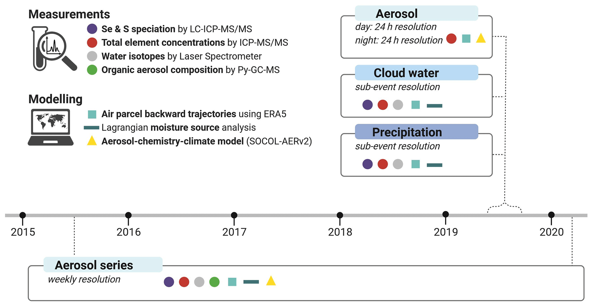
Figure 1Overview of the measurements and modelling approaches applied to the 2015–2020 aerosol time series and 2019 campaign, in which aerosol, cloud water, and precipitation samples were collected. Figure created with https://www.biorender.com/ (last access: 3 January 2024).
2.1.1 Weekly sampling of aerosols (2015–2020)
Two different systems were used to sample aerosols during warm (summer and autumn) and cold months (winter and spring). A total of 70 weekly aerosol samples were collected from June–October between 2015 and 2019 (referred to as warm-season samples) using a Tisch high-volume PM10 sampler located on the back side of the Bernard Lyot Telescope tower (south-west of the summit; distance of approximately 60 m from wet-deposition sampling). With this system, 8×10 in. quartz filters (QM-A, Whatman) were used after muffling them at 550 °C. The weekly sample collection of warm-season samples was conducted between specific times, i.e. from 22:00 to 15:00 UTC between the years 2015 and 2018 and from 20:00 to 08:00 UTC during 2019. Sampling throughout the entire day was not possible due to noise interferences of the high-volume sampler with the telescope observatory activities on the station. On average, warm-season samples were collected over 7±2 d with a collection volume of 7197±1816 m3. A total of 64 aerosol samples were collected from November through May between 2016 and 2020 (referred to as cold-season samples) using 90 mm single-stage Teflon filter packs (Savillex) with pre-muffled 90 mm diameter quartz filters (QM-A, Whatman). The filter packs, which were pre-cleaned before the campaign (with 10 % HNO3 and then ultrapure water), were connected to a Tekran 1104 Teflon-coated, heated manifold (necessary for sampling during cold temperatures). Ambient air was pulled through the manifold at a constant flow rate of ∼100 L min−1 using a blower unit. Total sampling volumes were recorded using gas meters that were installed at the outlets of the vacuum pumps (KNF™ aluminium–chromium diaphragm pump, ∼55 L min−1). On average cold-season samples were collected over 6.9±0.4 d (24 h d−1) with a collection volume of 518±32 m3.
2.1.2 High-temporal-resolution sampling of precipitation, cloud water, and aerosols (2019 campaign)
Precipitation and cloud water samples were collected on a (sub-)event basis at the aerology platform at Pic du Midi Observatory. Precipitation was sampled using two to three custom-made plastic (polypropylene) collectors that were pre-cleaned (with 10 % HNO3 and then ultrapure water) and only opened during precipitation events (surface area per collector: 0.159 m2). Cloud water samples were taken using a CASCC2 bulk fog–cloud sampler (air volume flow: 1470 m3 h−1) (Collett et al., 1990). Throughout the campaign, a total of 18 precipitation and 12 cloud water events were sampled, consisting of 26 and 58 sub-events, respectively. Aerosol filters were separately sampled during the day and night over 2 d (08:00/20:00 UTC, each 24 h in total) on 47 mm single-stage filter Teflon packs (Savillex, pre-burned filters: quartz QM-A Whatman) using the same system as described above for the collection of cold-season samples. The mean sampling volumes were 54±3 m3 over a collection period of 24 h.
2.2 Sample processing
2.2.1 Aerosol samples
All aerosol filters were collected and stored in aluminium foil in the dark at −20 °C. For the warm-season aerosol samples, two types of extractions were performed for (1) total element analysis (using microwave-assisted acid digestion) and (2) water-soluble Se and S speciation. This latter extraction was solely performed on the warm-season samples due to limited sample material and lower concentrations in the cold-season samples. For total element analysis (sub-samples 1), all aerosol samples were extracted with 4 mL HNO3 (69 %, ROTIPURAN® Supra, Roth) and 1 mL H2O2 (30 %, for ultra-trace analysis, Sigma-Aldrich) in a microwave oven (UltraCLAVE IV, MLS). The digestion programme of Kulkarni et al. (2007) was followed, which included a first temperature increase to 180 °C (15 min ramp, temperature held for 15 min) followed by a final increase to 210 °C (15 min ramp, temperature held for 45 min). Acid digestions of warm-season samples were performed using a 3.8 cm2 (filter area): 25 mL−1 (digestion volume) ratio. The digestion volume of cold-season samples was increased after 2017 from 5 to 15 mL to increase the available extraction volume for further analysis (final extraction ratio: 7.069 cm2 15 mL−1). For the water-soluble Se and S speciation analysis (sub-samples 2), all samples were extracted using a ratio of 11.404 cm2 (filter area): 15 mL−1 (ultrapure water volume). The filter : water suspensions were sonicated for 20 min at 20 °C (repeated twice), and the resulting extracts were filtered (0.22 µm, 25 mm syringe filters, nylon, BGB). A total of 9 mL of the extracts was used for pre-concentration and subsequent Se and S speciation, while the remaining sample volume was used for total element analysis to determine extraction efficiencies.
Furthermore, warm-season aerosol filters were analysed by Py-GC-MS to identify organic compounds previously used as proxies for aerosol sources (e.g. Zhao et al., 2009), for which 1.539 cm2 of aerosol filters was punched and folded into pyrolyzer cups (Eco-Cup SF, Frontier Laboratories, Japan).
2.2.2 Precipitation and cloud water samples
Precipitation and cloud water samples were processed within 2 h of collection. Snow and hail samples were thawed in closed sampling bottles before further processing. The total deposition amount of collected samples was determined by weight. At each sub-event, four sub-samples were taken for (1) quantification of total elements, (2) speciation of Se and S, (3) stable water isotopes, and (4) pH measurement. All plastic storage containers were pre-cleaned using 1 % HNO3, rinsed with ultrapure water, and air-dried. Sub-samples (1) used for total element quantification were filtered (0.22 µm, 25 mm syringe filters, cellulose acetate (CA), BGB), stabilized (1 % HNO3 of 69 %, ROTIPURAN® Supra, Roth) and stored at 4 °C until analysis. Sub-samples (2) used for speciation analyses were filtered (0.22 µm, CA), immediately frozen, and stored at −20 °C. Sub-samples (3) used for stable water isotope analysis were stored in closed airtight sampling bottles until resampling into PARAFILM-sealed glass vials within a few hours of collection. pH measurements were performed immediately after sampling with a field meter probe (Multi 3430 with pH electrode SenTix 940-3, WTW) that was calibrated daily. To enable pH measurement of wet-deposition samples, it was necessary to add a few drops of 3 mol L−1 KCl (Sigma-Aldrich) solution to sub-samples to increase ionic strength (Thermo Fisher, 2014).
2.3 Chemical analysis
2.3.1 Quantification of total element concentration
Total element concentrations (i.e. Li, Na, Mg, Al, Si, K, P, S, Ti, V, Cr, Mn, Fe, Co, Ni, Cu, Zn, As, Se, Br, Rb, Sr, Nb, Mo, Ag, Cd, I, Cs, Ba, Pb) were quantified using an Agilent 8900 ICP-MS/MS instrument equipped with an SPS 4 introduction system and using hydrogen (H2, 5 mL min−1, MS/MS mode), oxygen (O2, 30 mL min−1, MS/MS mode), and helium (He, 5.5 mL min−1, single quad) as reaction gases depending on the element (Supplement Sect. S1, Table S1). The instrument was tuned daily before analysis with a solution containing 10 µg L−1 of Mg, Li, Tl, Y, Co, and Ce. Instrument drift was monitored and corrected using internal standards (i.e. 1 mg L−1 Sc; 0.1 mg L−1 In, Lu; 50 µg L−1 Y; Supplement S1, Table S2). Instrument performance was checked with two certified reference materials for trace elements in surface waters with dilutions of 1:10 and 1:100 (SRM NIST 1643f; TMDA 51.2, National Water Research Institute, Environment Canada). Se yielded recoveries of 99±2 % for a concentration range of 0.12–1.20 µg L−1. Recoveries of other (trace) elements are listed in Supplement Sect. S1, Table S3.
2.3.2 Sample pre-concentration and determination of Se and S speciation
Sub-samples used for Se speciation analysis were pre-concentrated by lyophilization of frozen samples from an initial volume of 12 mL (for precipitation) or 9 mL (for water extract of aerosol filter) to a residual volume of 1.5 mL (pre-concentration factor of 8 or 6) to which ammonium citrate was added to increase ionic strength. The initial volume of cloud water samples was variable depending on sampled amounts. Further details on the optimized protocol and stability of Se species during pre-concentration are given in Supplement Sect. S2. S speciation was analysed directly in all atmospheric samples (i.e. without the pre-concentration step). Speciation of Se and S was analysed by high-pressure liquid chromatography (Agilent 1260 Infinity II Bio-Inert HPLC System) coupled to either an Agilent 8900 (Se speciation) or an Agilent 8800 (S speciation) ICP-MS/MS instrument. We optimized the chromatographic separations of Se species based on the method published by Tolu et al. (2011). The detailed optimizations of the chromatographic separation of Se are described in Supplement Sect. S3, including specific HPLC-ICP-MS/MS operating conditions for speciation analysis of Se and S (Supplement Sect. S3, Tables S5–S6). The optimized chromatographic method includes separation of Se species by anion exchange using a PRP-X100 column (Hamilton, 2.1×150 mm, 5 µm) equipped with an in-line filter (titanium frit 0.5 µm, 10-32 Waters type, BGB). Se separation was done by gradient elution with ammonium citrate (5.2–13 mM, 2 % MeOH, pH 5.2) delivered at 0.5 mL min−1 and an injection volume of 20 µL. For S, the chromatographic separation method developed by Müller et al. (2019) was applied, which includes gradient elution with formic acid (from 24 to 240 mM) delivered at 1 mL min−1 and an injection volume of 50 µL, using a Hypercarb column (100 × 4.6 mm, 5 µm, Thermo Fisher) equipped with guard column. For Se species detection, the ICP-MS/MS instrument operated in MS/MS mode with H2 as a reaction gas (5 mL min−1) and an acquisition time of 100 ms for all Se isotopes ( 74→74, 76→76, 77→77, 78→78, 80→80, and 82→82). To check for potential interferences, Br was monitored during all Se analyses (acquisition time: 50 ms; 79→79, 81→81). For S species detection, the ICP-MS/MS instrument operated in MS/MS mode with a mixture of O2 (30 %) and H2 (1 mL min−1) and an acquisition time of 50 ms for S ( 32→48). To monitor changes in sensitivity, a solution containing 30 µg L−1 of Y (acquisition time: 10 ms; 89→89) and 14 % tetramethylammonium hydroxide was continuously supplied post-column using the peristaltic pump of the ICP-MS/MS instrument. Both Se and S speciation analyses were measured in duplicate (i.e. two injections per sample).
All stock solutions of Se and S were prepared by weighing analytical-grade reagents and ultrapure water (18.2 mΩ cm, Thermo Fisher, Barnstead Nanopure Diamond) in acid-cleaned vials and were stored in the dark at 4 °C. The following standards were used: Se – selenite (SeIV, 99 %) and selenate (SeVI, 99.99 %), D,L-selenomethionine (SeMet, ≥ 99 %), and seleno-L-cystine (SeCys2, 95 %); S – dimethyl sulfoxide (DMSO, ≥ 99.9 %), dimethyl sulfone (DMSO2, ≥ 99 %), methanesulfonic acid (MSA, ≥ 99.5 %), methanesulfinic acid (MSIA, 85 %), sodium formaldehyde bisulfite (i.e. hydroxymethanesulfonate: HMS, 95 %), and sulfate (SO, 99 %). All standards were purchased from Sigma-Aldrich, except for SO and DMSO2, which were purchased from Merck. Stock solutions of SeCys2 were dissolved in 0.2 % HCl for stabilization purposes. Working standard solutions were prepared on the day of analysis by dilution in ultrapure water. Quantification of Se and S species was done by external species-specific calibration (i.e. mixed Se or S species standards prepared in the corresponding LC eluent). Data treatment was performed using the MassHunter 4.6 (Agilent) software. SeCys2 was used for the quantification of the “OrgSe” peak by anion exchange as further described in Sect. 3.2.1. Limits of detection (LODs) were calculated according to IUPAC recommendations; i.e. the LOD equals 3 times the standard deviation of the blank baseline signal divided by the calibration slope based on peak height.
2.3.3 Determination of organic compounds in aerosol samples
The analysis of organic compounds in aerosols was performed with a Frontier Lab pyrolyzer equipped with a Frontier Lab AS-1020E autosampler and connected to a Thermo Scientific TRACE 1310 GC instrument coupled to a Thermo Scientific ISQ 7000 MS instrument. The operating conditions and subsequent data processing method were according to Tolu et al. (2015) (see detailed description in Supplement S4).
2.3.4 Analysis of stable water isotopes
Stable water isotopes in precipitation and cloud water samples were measured using a wavelength-scanned cavity ring-down spectrometer (L2130-i, Picarro, Inc., Santa Clara, California, USA). Measurements and calibration were performed following the protocol by von Freyberg et al. (2022). Briefly, samples were injected six times, from which the first three were discarded to take into account potential memory effects. Measurements were calibrated to the Vienna Standard Mean Ocean Water 2 (VSMOW2)–SLAP scale as described by the International Atomic Energy Agency (IAEA, 2017). The isotopic abundances of 18O and 2H are reported using the δ notation relative to the IAEA standard VSMOW2 as described in Gat and Gonfiantini (1981).
2.4 Data and modelling
2.4.1 Particle number, black carbon, and observational meteorological data
A wide range of meteorological and other parameters characterizing the physical properties and chemical composition of the atmosphere at Pic du Midi Observatory are routinely monitored and are available through an internet database (https://p2oa.aeris-data.fr, last access: 21 April 2023). For this study, we used equivalent black carbon (BC) mass concentrations that were analysed by an Aethalometer (Magee Scientific AE33) with a time resolution of 15 min as described in Hulin et al. (2019). The particle number (PN) was analysed by a condensation particle counter (TSI, Inc., models 3010 and 3750) with a time resolution of 5 min. Meteorological data considered included air temperature (Vaisala QMH101), relative humidity, and atmospheric pressure (the latter two both measured with Vaisala MAWS301), which were all extracted with a time resolution of 60 min.
2.4.2 Air parcel back trajectories and moisture source analysis
To estimate dominant moisture sources of precipitation and atmospheric transport patterns, trajectories were calculated with the Lagrangian analysis tool LAGRANTO (Sprenger and Wernli, 2015; Wernli and Davies, 1997) with three-dimensional wind fields from the atmospheric reanalysis dataset ERA5 (Hersbach et al., 2020) interpolated to a 0.5° × 0.5° horizontal grid on 137 vertical levels. The air parcels' hourly positions (longitude, latitude, pressure) are calculated for 7 d backward in time from a set of five starting points including the location of Pic du Midi Observatory (42°56′11.4′′ N, 0°08′31.1′′ E) as well as four other points shifted by 0.5° in the horizontal to take into account uncertainties in the origin of air at the synoptic scale due to turbulent mixing in the boundary layer and the impact of orography. A set of variables is interpolated along the trajectories, namely, specific humidity and relative humidity, as well as the boundary layer height. Trajectories were started at the surface to assist in the interpretation of the aerosol data, as well as from a vertical stack of nine points every ∼ 80 hPa between 900 and 300 hPa for assessing the origin of precipitating air. The trajectories were started every hour for the 2019 campaign period and every 6 h for the climatological period between 2015 and 2020 for the aerosol time series.
The moisture sources of precipitation and cloud water were calculated using the algorithm developed by Sodemann et al. (2008). In short, the mass budget of water vapour in an air parcel is considered and moisture uptakes are registered whenever the specific humidity along an air parcel trajectory increases. The weight of each uptake depends on its contribution to the specific humidity of the trajectory upon arrival. If precipitation occurs underway (manifesting itself by a decrease in specific humidity along the trajectory) after one or several uptakes, the weight of all previous uptakes is reduced proportionally to their respective contribution to the loss.
The position and intensity of the precipitation systems in ERA5 are not always placed at the correct geographical location, in particular if they are of a convective nature. For example, no precipitating cloud may be present in ERA5 at Pic du Midi when precipitation was actually sampled. Therefore, we used a slightly different approach than Sodemann et al. (2008) to select precipitation and cloud water events. We based our event selection criteria on the actual precipitation and cloud water sampling and diagnosed the origin of water vapour during the respective sampling periods (similar to the approach in Aemisegger et al., 2014, and Pfahl and Wernli, 2008). For precipitation we use all available trajectories in the vertical column for which the relative humidity at arrival is close to saturation (> 80 %) during the sampling time interval, and for the cloud water samples we use near-surface water vapour. In both cases, we weight the contribution of individual moisture uptakes along each trajectory according to its specific humidity at arrival.
2.4.3 Chlorophyll a exposure in marine moisture source regions
To investigate a potential link between marine productivity and Se (speciation) in rainfall, chlorophyll a (Chl a) air exposure in marine moisture source regions was diagnosed with the same approach as in Suess et al. (2019). Sea surface water Chl a concentrations from the Ocean Colour Climate Change Initiative dataset, version 3.1 from the European Space Agency (available online at http://www.esa-oceancolour-cci.org/, last access: 21 June 2022), were used to estimate the air parcels' exposure to Chl a in marine moisture source regions. The chosen CHL-OC5 Chl a product (0.01° × 0.015° gridded data) is based on daily remote-sensing reflectance data of MODIS Aqua and MERIS Envisat. To minimize the impact of regions with missing data due to cloud cover in all seasons, 2-weekly composites were computed to estimate the time mean moisture source Chl a exposure. A similar approach to determining air exposure to marine Chl a was used in Blazina et al. (2017), with the difference that the exposure of the air was computed based on trajectory points located in the boundary layer. Here, we focus on Chl a exposure of air at instances when air parcels have taken up humidity along their paths. We thus use humidity uptake along the trajectories as an analogue for enhanced uptakes of biogenically derived compounds from the ocean to the atmosphere.
2.4.4 Data sources for thunderstorms
Lightning data were used to detect thunderstorm activity in the vicinity of Pic du Midi Observatory. Lightning maps (2-hourly) and data from the nearest radio antenna stations were extracted from the Meteo60 website (https://www.meteo60.fr/orages-archives/, last access: 24 November 2022), which takes its data from the Blitzortung network (list of stations: https://www.blitzortung.org/en/station_list, last access: 24 November 2022). Atmospheric deposition samples were classified as thunderstorm events if lightning activity was reported in the vicinity of Pic du Midi Observatory (within 3 km) during the time that a sample was collected. The vicinity was defined by comparing detected lightning with on-site observations during the 2019 campaign.
2.4.5 Atmospheric Se modelling with SOCOL-AERv2
We conducted 2015–2020 simulations in the aerosol–chemistry–climate model SOCOL-AERv2, which includes Se chemistry (Feinberg et al., 2019, 2020b). Selenium cycling is modelled with 7 gas-phase species, 40 particulate tracers in size bins between 0.39 nm and 3.2 µm, and 17 chemical reactions (Feinberg et al., 2020b). Global simulations are conducted at T42 horizontal resolution (2.8° × 2.8°) with 39 vertical levels up to 80 km. Model dynamical variables (vorticity and divergence of the wind fields, temperature, and surface pressure) are nudged towards ERA5 reanalysis data (Hersbach et al., 2019) in order to minimize the differences between observed and modelled meteorology in these simulations. Emissions of Se from anthropogenic, marine biogenic, terrestrial biogenic, and volcanic sources are considered, with emission totals constrained by a previous study applying Bayesian inference methods with available Se observations (Feinberg et al., 2020a). The SOCOL-AERv2 Se simulation has been thoroughly validated against available particulate and wet-deposition Se measurements (Feinberg et al., 2020a, b, 2021). The spatial distribution and trend in anthropogenic Se emissions are based on the CAMS-GLOB-ANT-v4.2 SO2 emissions inventory for 2015–2020 (Granier et al., 2019). The spatial distribution of marine biogenic emissions is calculated online by applying a wind-driven parametrization (Nightingale et al., 2000) to a marine dimethyl sulfide (DMS) climatology (Lana et al., 2011). Terrestrial biogenic emissions of Se are distributed following the mean monthly emissions of volatile organic carbon (VOC) emissions from the MEGAN–MACC inventory (Feinberg et al., 2020a; Sindelarova et al., 2014). Volcanic degassing emissions of Se are temporally constant and distributed according to the magnitude of volcanic SO2 emissions (Andres and Kasgnoc, 1998; Dentener et al., 2006). Selenium is removed from the atmosphere through wet- and dry-deposition parametrizations which depend on the calculated grid cell meteorology. Source tracking simulations were conducted by turning on only one of the four Se emission sources (anthropogenic, marine, terrestrial, or volcanic). Modelled particulate Se concentrations at the grid cell and altitude of Pic du Midi were extracted and compared to measured quantities.
2.5 Statistical analysis
All statistical analyses were performed using IBM SPSS Statistics 26. Principal component analysis (PCA) was performed on the precipitation data set given in mass per volume (g L−1) or per area (g m−2). Prior to the PCA, the data were converted to Z scores (average = 0, variance = 1). Principal components (PCs) with eigenvalues > 1 were selected and extracted using a varimax-rotated solution. A significance threshold value of > 0.39 was chosen. Other variables, e.g. precipitation volume, black carbon, and total column ice cloud water contents and moisture sources, were included passively in the PC-loading plots using bivariate correlation coefficients between these variables and the PC scores of each PC. Correlations were performed as Spearman rank correlations (correlation coefficient indicated by rS). Significance levels (two-tailed) of performed correlations are indicated by p<0.05 or p<0.01.
3.1 Factors driving total Se deposition fluxes
3.1.1 Variability in total Se concentrations and source contribution of Se in aerosols
In a first step, we investigated Se concentrations in aerosols taken at a weekly resolution over 5 years (2015–2020) to gain insights into the synoptic-timescale variability in total Se deposition at Pic du Midi Observatory and how this is affected by different sources. Total Se concentrations (after digestion using HNO3 and H2O2) ranged from 2 to 221 pg m−3 in the 2015–2020 aerosol time series (n=134; average: 58±57 pg m−3; median: 33 pg m−3; Fig. 2 and in Supplement Sect. S5, Fig. S4). We clearly see higher Se concentrations in summer (June–August; average: 114±50 pg m−3; median: 111 pg m−3) than during spring (March–May; average: 32±24 pg m−3; median: 30 pg m−3), autumn (September–November; average: 49±44 pg m−3; median: 27 pg m−3), and winter (December–February; average: 9 ± 5 pg m−3; median: 9 pg m−3). Similar seasonal differences, with the highest Se levels in summer, were also observed in an aerosol time series collected at the Neumayer station in Antarctica (Weller et al., 2008), for which the authors suggested that this seasonal trend is driven by biogenic Se emissions. In our study, we compared Se concentrations to many other (trace) elements, and most of them show a similar pattern with higher concentrations in summer (see data for S, Fe, and Pb in Supplement Sect. S5, Fig. S5). This is interesting as it is likely that these elements are derived from different sources, e.g. mineral dust (e.g. Fe and Mn) or anthropogenic activities (e.g. Pb), which would indicate that elemental concentration patterns are driven by not only sources but also other (physical) processes. Higher aerosol loadings are likely related to direct exports from the boundary layer through convection or by anabatic (i.e. upslope or valley) wind systems (Hulin et al., 2019).
To determine the main Se source contributions of the 2015–2020 aerosol time series, we used the aerosol–chemistry–climate model SOCOL-AERv2. It should be noted that model grid cells represent an area of km2, which is much larger than our sampling site, and thus give regionally averaged rather than site-specific information. The SOCOL-AERv2 model identifies four major Se sources: anthropogenic, volcanic, marine, and terrestrial sources (Fig. 2). We found that proportions of terrestrial contributions are highest in summer with 41±7 % (of total estimated sources) followed by autumn (21±10 %) and spring and winter (both 9±4 %), as can be expected from a previous study conducted at Pic du Midi (Suess et al., 2019). In contrast, marine sources are more important in spring (53±20 %) and winter (48±14 %) compared to autumn (34±15 %) and summer (24±7 %). Anthropogenic and volcanic sources (for our study site this is mainly the Etna volcano in Sicily) do not show clear seasonal variations, with average contributions of 32±8 % and 8±10 %, respectively.
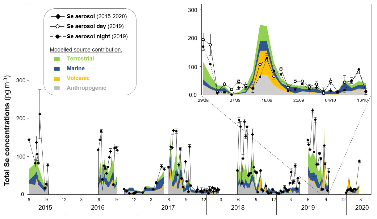
Figure 2Comparison of Se aerosol measurement with modelled Se data. Data shown for 2015–2020 aerosol time series (filled diamonds) as well as day (outlined circles with continuous line) and night (filled circles with dashed line) aerosol measurements in the 2019 campaign (campaign period shown in top-right corner). Modelled source contributions by SOCOL-AERv2 are shown as stacked areas, including biogenic terrestrial (green), marine (blue), volcanic (yellow), and anthropogenic (grey) activities.
Overall, the agreement between the weekly Se measurements in the 2015–2020 aerosol time series and the model is high (rS=0.822; Supplement Sect. S6, Fig. S6). A previous SOCOL-AERv2 evaluation found similar correlation values (r∼0.8) in a spatial comparison with annual means from measurement stations worldwide (Feinberg et al., 2020a). Our comparison here with higher-time-resolution measurements acts as an additional test of the model's ability to capture the temporal variability in Se sources and transport. The overall good correlation provides confidence in the model's predictions of Se source contributions at Pic du Midi Observatory. For example, lower Se concentrations (< 0.05 ng m−3) are well captured by the model and are predominantly characterized by marine source contributions (Fig. 2 and in Supplement Sect. S6, Fig. S7b). However, the model displays a negative bias (−0.016 ng m−3), underestimating the higher Se concentrations (> 0.05 ng m−3) observed in summer (Fig. 2). Such a bias is to be expected when comparing a relatively coarse global model simulation with observations from a mountain station. At the horizontal grid spacing of 300 km, the model does not capture the complex terrain and associated boundary layer dynamics around Pic du Midi that lead to enhanced boundary layer contributions and higher aerosol loadings. In addition, a model grid point value always represents an area average, in contrast to point measurements. Particularly terrestrial source contributions seem to be underestimated (Supplement Sect. S6, Fig. S7a), whereas volcanic source contributions tend to be overestimated by the model (particularly during the 2019 campaign period in Fig. 2 and Supplement Sect. S6, Fig. S7c). This discrepancy is likely related to the (spatially and temporally) dynamic nature of volcanic emissions. So far, the model only considers constant Se degassing emissions from volcanoes with a globally uniform Se:SO2 emission ratio due to very limited availability of emission data (Feinberg et al., 2020a).
The aerosol data are thus useful to understand seasonal variability in Se concentrations; however, Se deposition to the surface occurs predominantly via wet deposition (∼ 80 %) (Wen and Carignan, 2007; Feinberg et al., 2020a), and therefore it is also important to further understand what drives concentrations in wet deposition.
3.1.2 Variability in elemental concentrations and moisture sources in wet deposition
During the campaign in 2019, total Se concentrations in precipitation ranged from 12 to 84 ng L−1, resulting in total Se deposition of 11 to 428 ng m−2 (n=26, average 42±21 ng L−1 and 85± 92 ng m−2, respectively; Supplement Sect. S5, Fig. S4). It should be noted that concentrations in aerosols and wet deposition cannot be directly compared because they are given in different units. These Se concentrations are similar to ranges reported for precipitation at remote and/or continental sites (6–85 ng L−1; Suess et al., 2019; Roulier et al., 2021) and the open ocean (20–40 ng L−1; Pacific – Arimoto et al., 1985; Atlantic Ocean – Cutter, 1993, and Cutter and Church, 1986). They are, however, much lower than the Se concentrations found at coastal sites (310–2830 ng L−1; Blazina et al., 2017) and urban sites (50–1010 ng L−1; Tokyo, Japan – Suzuki et al., 1981; Sri Lanka – Savage et al., 2017). Selenium concentrations in cloud water ranged between 0.018 and 0.967 µg L−1, corresponding to 1–16 pg m−3 (n=56 samples, 5±4 pg m−3; Supplement Sect. S5, Fig. S4). To the best of our knowledge, there have been no previous studies on Se concentrations in cloud water in Europe. Only a small number of samples have been collected at mountain sites in Japan (Kagawa et al., 2022), Pakistan (Ghauri et al., 2001), and the USA (Richter et al., 1998; Yang and Husain, 2006), with higher Se concentrations (0.2–9.2 µg L−1) that the authors related to anthropogenic sources.
To investigate potential parallels between trace element cycling and the atmospheric water cycle, we studied the variability in elemental concentration in wet deposition under different contributing moisture sources and used water isotope signals as indicators of precipitation formation conditions. Precipitation and cloud water samples collected at Pic du Midi were influenced by both land and oceanic moisture sources with approximately equal contributions for both sample types (Supplement Sect. S7, Fig. S8). Most precipitation samples were characterized by high contributions of more remote moisture sources coming from the North Atlantic (precipitation events: P2–P5, P13–P18; average moisture contribution: 58 ± 17 % versus 8 ± 7 % in other events) or northern Africa (P6–P10; average moisture contribution: 26 ± 9 % versus 1 ± 1 % in other events). In contrast, most cloud water samples were predominantly influenced by regional sources (Spain north of 41.8° N and France south of 43.6° N; C1–C3, C8–C10; average moisture contribution: 51 ± 12 % versus 34 ± 15 % in other events), with remaining events showing high contributions from the North Atlantic (C4, C9, C11; average moisture contribution: 69 ± 8 % versus 35 ± 19 % in other events). The isotope signatures in precipitation (δ2H = −45.4 ± 15.6 ‰ and δ18O = −7.6 ± 1.9 ‰) showed a larger and more depleted range than cloud water (δ2H = −26.7 ± 13.4 ‰ and δ18O = −5.3 ± 1.6 ‰), which is likely due to higher precipitation formation altitudes with the contributing air being more depleted due to the rainout effect with increasing height (Dansgaard, 1964). In cloud water, we observed a positive correlation between water isotopes and concentrations of Se (p<0.01) as well as with almost all analysed (trace) elements, except for Si (δ2H: p=0.054) and Fe (δ2H: p=0.046), which are mineral dust indicators. This correlation, which seems to mainly arise from cloud water events with regional moisture sources (Supplement Sect. S7, Fig. S9), was not observed for precipitation (Supplement Sect. S7, Fig. S10). The link between (trace) elements and water isotopes in cloud water is likely explained by the predominantly regional/local sources (in a 0.5° radius around Pic du Midi Observatory) of both trace elements and atmospheric water, except for mineral dust (Si, Fe), which is derived from longer-distance sources. In the case of precipitation, low δ2H and δ18O indicate a loss in heavy water isotopes during long-range transport (e.g. due to rainout or mixing of air underway). Below-cloud processes may further alter trace element and water isotope signals in precipitation, including (i) below-cloud scavenging of aerosols containing trace elements and (ii) rain droplet evaporation and equilibration, which may lead to a pre-concentration of elements and complex alteration of the isotopic signatures. These processes lead to a decoupling of transport pathways for stable water isotopes and (trace) elements in precipitation in contrast to cloud water.
3.1.3 High Se and other element deposition associated with deep convective activity during thunderstorms
To gain a better insight into processes affecting Se concentrations in wet deposition, we analysed chemical and physical characteristics of precipitation events sampled during the campaign in 2019. Even though our study focuses on Se, we also investigated other (trace) elements in wet deposition which have been used as source indicators in previous studies, e.g. mineral dust (e.g. Fe and Mn) or anthropogenic activities (e.g. Pb).
During this campaign, different (mixed) precipitation types including rain, hail, snow, sleet, light rain, and/or cloud water (fog) were collected with precipitation rates ranging between 0.1 and 10.2 mm h−1; the highest rates occurred during events that included hail (Supplement Sect. S7, Table S8). Variability in both elemental concentrations in precipitation (given in µg L−1) and deposition fluxes (given in µg m−2) was explored using principal component analysis (PCA). Elemental concentrations in precipitation are expected to be influenced by the dilution effect (Gatz and Nelson Dingle, 1971), which predicts lower concentrations for increasing rain volumes. While many major and trace elements (e.g. Na, K, P, Fe, Cu, Zn, As, Pb) showed a significant negative correlation with precipitation (p<0.05), Se concentrations did not significantly decrease with increasing precipitation amount. To the best of our knowledge, the role of different precipitation types in this effect has not been investigated before. Our data suggest that for events with light rain and/or cloud water, concentrations of the majority of analysed (trace) elements are significantly affected by precipitation volume, while no effect was observed for other precipitation types (PCA description in Supplement Sect. S8.1).
Element deposition fluxes (in µg m−2, not influenced by the dilution effect) were generally high between 14 and 19 September 2019 with two characteristic maxima for most (trace) elements (events P8 and P11.1, highlighted by a vertical line in Fig. 3a). The precipitation events with high elemental deposition (P6–P11) plot on the positive side of the first principal component (PC1: 42 % of total variance; Fig. 3b), indicating similar source or process factors. A positive correlation to PC1 groupings was observed for moisture sources coming from northern Africa (p<0.01, Fig. 3b) as well as the western Mediterranean, which is expected as it follows the same trajectory from Africa to Pic du Midi. During this period we visually observed a brownish-red colour of collected samples (i.e. precipitation P7–10, cloud water C5, and aerosols A9–A11) as well as higher pH values in precipitation (pH 6.2–7.2 in P8–P10 versus pH 5.4–5.8 in all other events), which is a known effect of dust deposition during so-called “red rains” (Chester et al., 1996), indicating increased dust loadings. Furthermore, these events were characterized by significantly higher contents of black carbon (BC; Mann–Whitney U test, p<0.01) and total column ice water contents (TCIW given in mm, integrated over the troposphere from the ERA5 reanalysis dataset; Supplement Sect. S8.2, Fig. S12), which both positively correlate with PC1 groupings (p<0.01; Fig. 3b). Both mineral dust and BC aerosols are known to play an important role in heterogeneous nucleation by acting as effective ice-nucleating particles (Kanji et al., 2017). Apart from the presence of dust, BC, and TCIW, precipitation events with high elemental deposition in this period were associated with thunderstorms (thunderstorms identified both from visual observations during sampling and from lightning data of the Blitzortung's network; Mann–Whitney U test, p<0.01; Supplement Sect. S8.2, Fig. S13). PC scores of sub-events classified by their precipitation type, including events with rainwater/hail, light rain/cloud water, snow/sleet, or thunderstorms, show groupings on PC1 and PC2. Particularly sub-events with thunderstorms show positive PC scores on PC1, which indicates a significant influence of this factor on the element grouping of PC1 (Fig. 3c). Thunderstorms were predominantly related to continental moisture sources (70 % versus 46 % in non-thunderstorms) and much less to Atlantic moisture sources (7 % versus 47 % in non-thunderstorms). With respect to the higher elemental contents in wet deposition, thunderstorm clouds extend to the upper troposphere and are generally characterized by higher rainfall rates and larger rain droplets (Tost et al., 2006), leading to efficient below-cloud scavenging of aerosols. A previous study observed high mercury (Hg) concentrations in wet deposition during thunderstorms in the eastern United States, which the authors explained by scavenging of gaseous HgII and HgII aerosols in updraughts and downward mixing of tropospheric Hg (as HgII) to lower altitudes (Holmes et al., 2016).
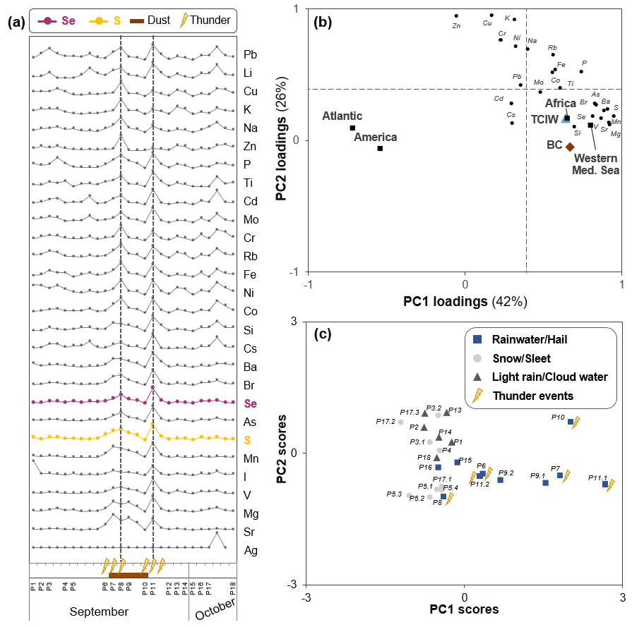
Figure 3Precipitation chemistry and (sub-)event characteristics. (a) Variability in concentrations of all measured elements in precipitation collected during the 2019 campaign. (b) Loading and (c) score plots for PC1–PC2 of the elemental deposition dataset. Four PCs were retained, i.e. PC1, 42 %; PC2, 26 %; PC3, 25 %; and PC4, 2 % of total variance. For the PC loadings, black circles correspond to active variables, and the variables black carbon (BC, brown diamond) and total column ice water contents (TCIW, blue triangle) as well as moisture sources (including the Atlantic, America, Africa and the western Mediterranean Sea, shown as filled squares) were added passively (p<0.01). The significance level of > 0.39 is indicated by dashed horizontal and vertical lines in the loading plot. Additional information on precipitation events in (a) and (c) includes the following: observed dust colour in samples (brown bar), thunderstorms (lightning bolts), and precipitation type (rain/hail: blue squares; snow/sleet: light-grey circles; light rain/cloud water: dark-grey triangles). Two significant elemental deposition increases discussed in the text are highlighted by dashed lines in (a).
In a next step, we investigated the importance of thunderstorms for elemental concentration trends in aerosols in the 2015–2020 time series. Also for this dataset, elemental concentrations in aerosols were significantly higher during weeks in which thunderstorms occurred than for samples that were not related to thunderstorms (selection of major and trace elements in Fig. 4; Mann–Whitney U test, p<0.01; data for all analysed elements in Supplement Sect. S8.3). For Se, these highest concentrations were generally underestimated in the SOCOL-AERv2 model (Supplement Sect. S8.3, Fig. S16). Significantly higher elemental concentrations associated with thunderstorms were observed not only when considering the full aerosol time series, but also when only considering measurements in summer (Mann–Whitney U test, p<0.05 except p=0.06 for Ni and p>0.2 for Ti, Zn, and Mo; Supplement S8.3, Table S9), during which average concentrations are generally higher. Higher elemental concentrations are a clear indicator of higher aerosol loadings. Previous studies have suggested that high aerosol loading may trigger a chain of processes that ultimately increase the strength of convective updraughts. Related to this, higher frequencies of lightning have been linked to high aerosol loadings (Williams and Stanfill, 2002; Zhao et al., 2015; Thornton et al., 2017; Pan et al., 2022). Within the cloud and updraughts, condensed water and ice can efficiently scavenge soluble gases and aerosols containing elements (as previously observed for Hg; Holmes et al., 2016). Notably, we found a positive correlation between the occurrence of thunderstorms and the absolute humidity at Pic du Midi (Supplement Sect. S8.3, Fig. S17). Higher humidity likely favours stronger convection and finally wash-out of aerosols via precipitation.
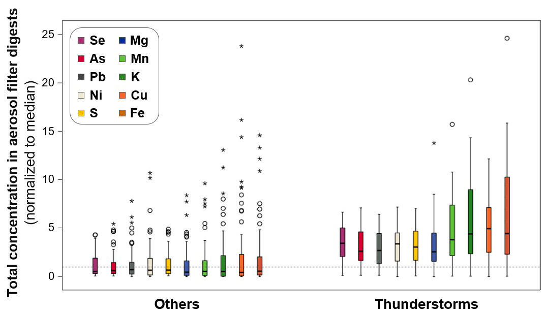
Figure 4Comparison between normalized total concentrations of different major and trace elements in aerosol filter digests sampled during weeks with thunderstorms (right side). All other aerosol measurements without detected thunderstorms during sampling are shown on the left (“Others”). The total concentrations shown were normalized by the median of the respective element (values equal to the median indicated as a horizontal dashed line; y=1). All shown aerosols measurements during weeks with thunderstorms are significantly different (Mann–Whitney U test; p< 0.01).
Apart from the finding that deep convective activity during thunderstorms leads to significantly higher elemental deposition, thereby impacting the supply of micronutrients and potentially toxic elements to the surface, our results imply that high elemental concentrations do not necessarily indicate a source signal in deposition data. More specifically, our data suggest that while element concentrations in the atmosphere may be primarily determined by the element fluxes at the source, local cloud dynamics of different weather events control the amounts of Se and other (trace) elements in atmospheric deposition fluxes. This implies that variability in elemental concentrations in wet deposition reflects not only changes in strengths of emission sources alone but also weather conditions during atmospheric removal.
3.2 Factors driving the deposited chemical form of Se
We further investigated the chemical forms (speciation) of Se in atmospheric samples and compared these to speciation data for S to further investigate potential source signatures. Furthermore, speciation in atmospheric deposition is relevant for the bioavailability of Se delivered via rainfall to soils and crops, as elemental speciation is an important factor for plant uptake and mobility in soils.
3.2.1 Detection of inorganic and organic Se species
To determine Se speciation in atmospheric samples at ultra-trace levels, we developed (1) an extraction method for the water-soluble fraction of aerosols; (2) a pre-concentration method based on volume reduction by lyophilization, which was applied to aerosol water extracts, precipitation, and cloud water; and (3) an optimized LC-ICP-MS/MS method (detailed procedure in the Methods section and in Supplement Sect. S2–3). Our optimized procedure reaches a detection limit of 1–2 ng L−1 depending on the Se species, which is 5 to 10 times lower than existing methods (Suess et al., 2019; Roulier et al., 2021). Thus, we could detect not only the oxyanions SeIV and SeVI in all sample types, but also a third Se peak that is likely of organic nature, here further defined as OrgSe (see chromatograms in Supplement Sect. S9, Fig. S18a). Further analysis using a cation exchange column showed several unknown peaks, with one found to co-elute with an in-house synthesized standard of the metabolite dimethylselenonium propionate (DMSeP), which could indicate that this peak consists of small methylated Se compound(s) (Supplement Sect. S9, Fig. S19). With our method, Se species recoveries accounted for 65 ± 13 % of total Se concentrations in aerosol water extracts, 77 ± 14 % in cloud water, and 66 ± 10 % in precipitation (Supplement Sect. S9, Fig. S20). Previous studies solely detected inorganic Se, mostly SeVI (SeIV being below detection limits in 89 %–96 % of samples) and had much lower Se species recoveries (20 %–42 %) (Suess et al., 2019; Roulier et al., 2021). To achieve full identification of the organic Se species, high-resolution mass spectrometry may further be used given that sufficient pre-concentration can be reached.
Average concentrations of SeVI, SeIV, and OrgSe accounted for 44 ± 28 pg m−3, 5 ± 4 pg m−3, and 3 ± 2 pg m−3 in aerosol water extracts; 3 ± 2 pg m−3, 0.7 ± 0.8 pg m−3, and 0.3 ± 0.2 pg m−3 in cloud water; and 44 ± 55 pg m−2, 10 ± 10 ng m−2, and 2 ± 2 ng m−2 in precipitation, respectively. We investigated proportions of Se species rather than absolute concentrations for further data analysis to allow comparison between different atmospheric samples, since the use of species proportions removes influences by, for example, variability in aerosol loading or precipitation volume (dilution effect) among specific seasons and events. The main Se species in all analysed atmospheric samples is SeVI, followed by SeIV and OrgSe (Fig. 5). SeVI accounts for 53 ± 13 % (aerosol), 49 ± 13 % (precipitation), and 63 ± 14 % (cloud water) of total Se concentrations, while SeIV represents 8 ± 8 % (aerosol), 13 ± 12 % (precipitation), and 15 ± 9 % (cloud water) of total Se concentrations. OrgSe accounts for the smallest fraction with 3 ± 2 % (aerosol), 4 ± 2 % (cloud water), and 2 ± 1 % (precipitation) of total Se concentrations (Fig. 5). Besides Se species, we detected the S species sulfate (SO and methanesulfonic acid (MSA), as can be expected in atmospheric samples. We could also detect dimethyl sulfone (DMSO2) and hydroxymethanesulfonate (HMS) (see chromatograms in Supplement Sect. S9, Fig. S18b). To ensure correct quantification of MSA and HMS, which elute very close to each other, species-specific calibration standards (i.e. mixed S species standards) were used.
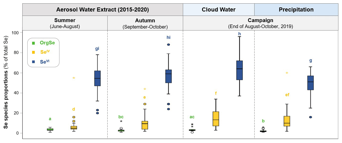
Figure 5Variability in proportions of Se species in different collected atmospheric samples. Se species shown include the following: OrgSe (green), SeIV (yellow), and SeVI (blue) in the water extracts of 2015–2020 aerosol time series as well as precipitation and cloud water collected during the campaign in 2019. Se speciation in aerosols is separately displayed for summer (June–August) and autumn (September–October). The letters (a)–(i) denote significant differences in species proportions (Mann–Whitney U test; p<0.01).
3.2.2 Inorganic Se speciation is influenced not only by the emission source but also by pH
To get insights into processes and/or sources affecting inorganic Se in atmospheric deposition, we investigated the species variability in different atmospheric samples and their potential links to different source indicators. Figure 5 shows the proportions of Se species (percent of total Se concentrations) in the water extracts of the 2015–2020 aerosol time series as well as in precipitation and cloud water from the campaign in 2019. No clear seasonal differences were observed for proportions of SeVI, but SeIV had significantly lower proportions in aerosol samples collected in summer (7 ± 7 %) than in autumn (11 ± 9 %).
To test for potential sources of inorganic Se, we studied correlations between inorganic speciation, moisture sources, and Py-GC-MS data in aerosols. For the 2015–2020 aerosol time series, proportions of SeVI positively correlate with continental moisture sources from Spain (rS=0.263, p<0.05), Portugal (rS=0.327, p<0.01), and northern Africa (crossing over the Mediterranean Sea, rS=0.336, p<0.01). Furthermore, SeVI proportions positively correlate with both aliphatic and aromatic compounds (p<0.05), which have been linked to various continental sources, including both urban/anthropogenic and biogenic land emissions (e.g. Zhao et al., 2009). Proportions of SeIV showed no link to moisture sources but positively correlate with proportions of HMS (rS=0.509, p<0.01) and SO (rS=0.440, p<0.01). HMS is formed in an aqueous-phase reaction between formaldehyde and dissolved sulfur dioxide (e.g. Dovrou et al., 2019). Proportions of HMS positively correlate with continental moisture sources from western Europe (p<0.01), particularly France (local source, in France south of 43.6° N). The link between SeIV and HMS may indicate an anthropogenic source contributing to the SeIV signal in aerosols. This is also suggested from the positive correlation of SeIV proportions with the abundance of (poly)aromatics (rS=0.434, p<0.01), toluene (rS=0.312, p< 0.05), and S compounds (rS=0.353, p< 0.01; Supplement Sect. S10, Table S10). Indeed, toluene and alkyl-substituted benzenes identified by Py-GC-MS have been previously linked to kerogen and black carbon (Zhao et al., 2009). Besides this, SeIV proportions negatively correlate with Py products of proteins (, p<0.05) and levoglucosan (, p<0.01), indicating no link to fresh biomass and/or biomass burning (Fraser and Lakshmanan, 2000; Giannoni et al., 2012; Fabbri et al., 2008; Schkolnik and Rudich, 2006). To summarize, higher proportions of SeVI in aerosols were related to continental moisture sources and Py compounds from land emissions, whereas for SeIV, a likely anthropogenic contribution was observed.
Contrary to what we found for aerosols and to previous observations for precipitation samples by Suess et al. (2019), the proportions of SeVI in precipitation showed no link to continental sources, which is likely related to the limited number of precipitation events during our campaign with predominant moisture sources from western Europe. Sub-events that showed relatively high proportions of SeIV (28 %–60 %) in precipitation were characterized by higher moisture uptakes over coastal northern Spain (P16–P17.1, Fig. 6a, b). Particularly coastal marine emissions seem to influence the SeIV signal according to the observed correlation with coastal oceanic moisture uptakes (within 30 km of the coast, only considering uptakes over the ocean; rS=0.411, p<0.05). Notably, these relatively high SeIV proportions changed significantly during sub-events (see evolution of SeIV proportions during P17 in Fig. 6b and relative changes in moisture sources during sub-events in Fig. 6c). No HMS was detected in sub-events that showed relatively high proportions of SeIV, indicating a different origin of SeIV in wet deposition than for the 2015–2020 aerosol dataset.
The long-term weekly resolved aerosol and high-resolution precipitation data thus indicate different sources for SeIV. The 2015–2020 aerosol time series mainly has an anthropogenic signature of SeIV, whereas the (sub-)event-based sampling in 2019 enabled the elucidation of other sources and processes. In particular, marine coastal emissions (potentially in relation to sea spray emission) seem to contribute to higher SeIV proportions in wet deposition.
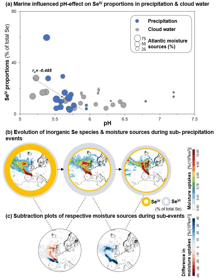
Figure 6Inorganic Se speciation in precipitation and cloud water as a function of dominating moisture sources. (a) Proportions of SeIV (% total Se) as a function of pH in precipitation (blue circles) and cloud water (grey circles) during the high-resolution campaign in 2019. The size of data points corresponds to proportions of Atlantic moisture sources (% total moisture sources). (b) Evolution of proportions of inorganic Se species, SeIV (yellow) and SeVI (grey), during sub-precipitation events (P17.1: 270 min; P17.2: 380 min; P17.3: 110 min duration) with corresponding moisture source plots (shown in colour scale 0 %–10 % per 105 km2). (c) Subtraction plots of relative moisture source changes (shown in red–blue colour scale from −40 % to 40 % per 105 km2) during sub-precipitation events shown in (b).
Although we can link inorganic Se speciation to specific marine/coastal sources, we further found an effect of pH in wet deposition (pH in aerosols was not determined). Oxidation-reduction reactions are strongly influenced by the redox potential (pe) and pH in natural waters. From the pe–pH stability field diagram (Séby et al., 2001), it is clear that the speciation of Se is likely quite sensitive to pH under atmospheric conditions. For a redox potential of pe ∼ 10 (range of rainwater pe: 8–11; Willey et al., 2012), SeIV is the thermodynamically favoured species at acidic pH values (∼ 2.5–5.5), whereas SeVI is favoured for pH values > 6 (Séby et al., 2001). Figure 6 shows the proportions of SeIV in relation to the pH of precipitation (blue circles) and cloud water (grey circles). Precipitation and cloud water with predominantly Atlantic moisture sources (the size of data points corresponds to percentages of Atlantic moisture sources) show a negative correlation between pH and SeIV proportions (, p<0.05), indicating a marine-influenced pH effect on Se speciation in precipitation and cloud water. Although sea salt aerosols are generally thought to be in the alkaline pH range (Pye et al., 2020), a recent study showed that pH values of freshly emitted sea spray aerosols are significantly lower than that of seawater (approximately pH 4 versus pH 8), with even lower pH values for aerosol particles below 1 µm in diameter (Angle et al., 2021). Thus, the observed link between pH and SeIV proportions in precipitation events with predominantly Atlantic moisture (Fig. 6a) might be related to the influence of sea spray. To further investigate the potential influences of atmospheric sources on inorganic Se speciation, we did a literature review of previously reported ratios of SeIV to SeVI and classified the sampling sites into urban, industrial, marine, forested area, and remote (Fig. 7). Higher proportions of SeIV have been reported in urban, industrial, and marine environments (SeIV: SeVI=2.2 ± 2.4) compared to the precipitation samples collected at Pic du Midi (this study; SeIV: SeVI=0.4 ± 0.7) as well as ratios reported in remote and forested areas (SeIV: SeVI=0.4 ± 0.3). Despite the small number of samples in the study referred to, the relatively high ratios previously reported in a marine environment (western North Atlantic) (Cutter and Church, 1986) agree with our observations above, i.e. higher proportions of SeIV for precipitation events with predominantly Atlantic moisture.
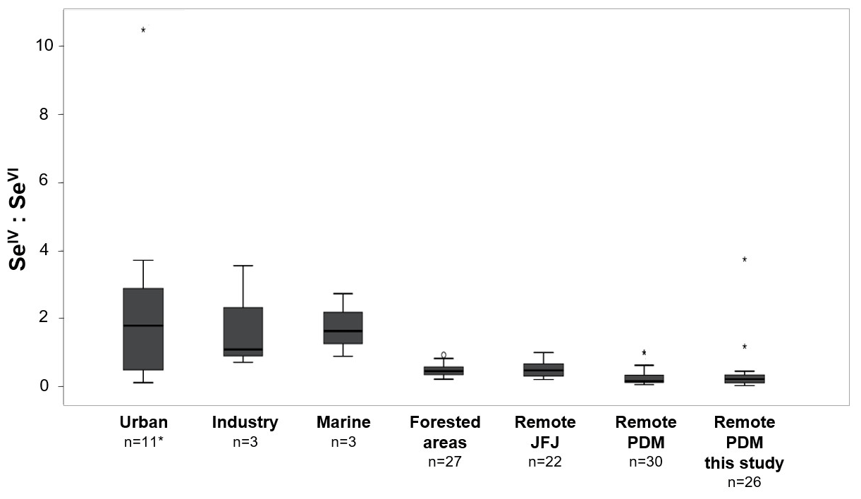
Figure 7Previously reported ratios of SeIV to SeVI concentrations classified by sampling sites: urban, industry, marine, forested area, remote. The number of data points indicated for each source class is indicated by n. *Urban data derived from five different studies (Cutter, 1978; Cutter and Church, 1986; Wang et al., 1994; Wallschläger and London, 2004; Donner and Siddique, 2018). Other classifications comprise data from industrial (De Gregori et al., 2002), marine (Cutter and Church, 1986), and forested areas (Roulier et al., 2021). Remote data refer to this study and the previous study of Suess et al. (2019) conducted at two high-altitude stations: Jungfraujoch (JFJ, Switzerland) and Pic du Midi (PDM, France).
3.2.3 Sources of organic Se
We further investigated potential source signatures of the OrgSe fraction in the 2015–2020 aerosol time series. Proportions of OrgSe in aerosols collected in summer (3.5 ± 1.3 %) had higher proportions than aerosols collected in autumn (2.8 ± 2.0; Fig. 5). Similarly to OrgSe, higher MSA concentrations were observed in summer compared to autumn (i.e. 5.3 ± 2.5 versus 2.3 ± 1.3 ng m−3), and the proportions of MSA and OrgSe (rS=0.369, p<0.01) correlate significantly, suggesting that OrgSe may originate from a similar biogenic source to MSA, which is an oxidation product of DMS (Chen et al., 2018).
To further investigate a potential biogenic source of OrgSe in aerosols, we studied links to dominant moisture sources and other organic compounds identified by Py-GC-MS. Proportions of OrgSe in the water-soluble aerosol extracts correlate with Atlantic moisture sources (rS=0.242, p<0.05), similarly to MSA (rS=0.328, p<0.01). Furthermore, the proportions of OrgSe positively correlate (rS=0.532, p<0.01; Supplement Sect. S10, Table S10) with the relative abundance of Py products that are specifically derived from proteins and amino acids (i.e. 2,5-diketopiperazine, denoted DKP; Voorhees et al., 1997, 1992; Fabbri et al., 2012).
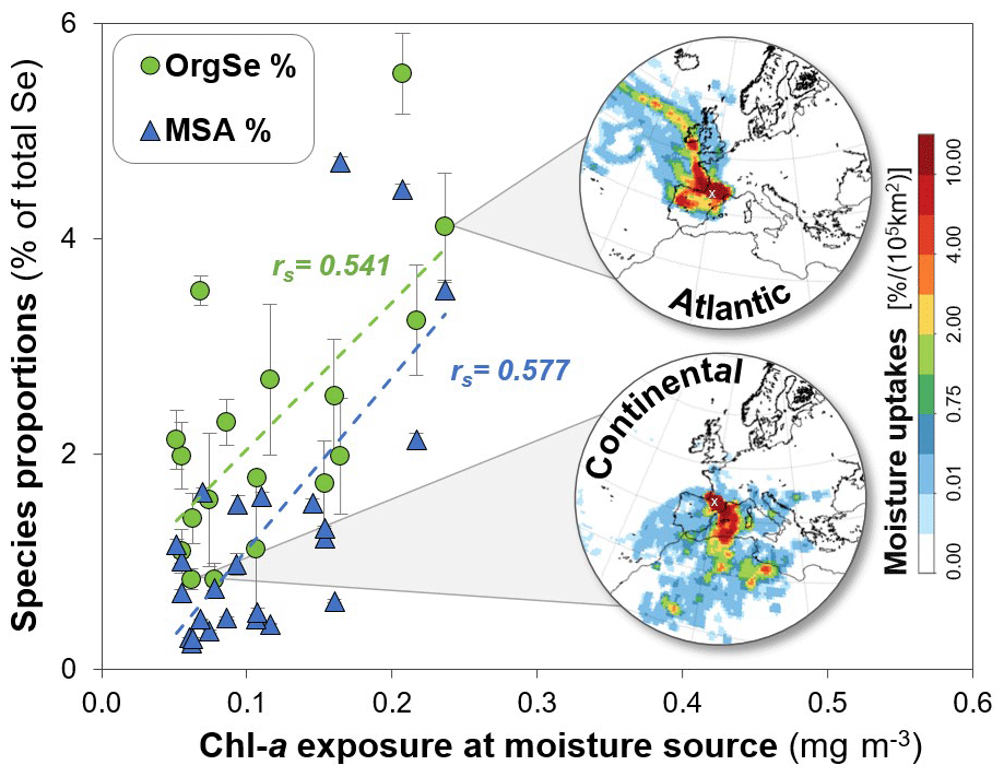
Figure 8Proportions of OrgSe (green circles) and MSA (blue triangles) as a function of Chl a exposure at the moisture source of precipitation. Two examples of low and high values of OrgSe proportions are shown with corresponding moisture plots. The example of high OrgSe proportions shows high-Atlantic-moisture sources (37 % of total moisture sources, P5.2), whereas the low-OrgSe example is dominated by continental moisture (22 % northern Africa and 44 % western Europe, P9.2). It should be noted that moisture uptakes are displayed as percentage uptakes per area (105 km2); thus depending on the defined size of areas, high moisture uptakes (red) do not necessarily correspond to predominant sources. The error bars represent the standard deviation values resulting from quantification by LC-ICP-MS/MS in duplicate.
For the precipitation and cloud water samples collected during the campaign in 2019, there is no significant correlation between the proportions of OrgSe and Atlantic moisture sources, in contrast to MSA (rS=0.705, p<0.01) and DMSO2 (rS=0.730, p<0.01). Instead, the proportions of OrgSe and chlorophyll a (Chl a) exposure at the moisture source (rS=0.541, p< 0.05; Fig. 8) are significantly correlated. Both MSA (rS= 0.577, p< 0.01; Fig. 8) and DMSO2 (rS= 0.494, p< 0.05) also show significant correlations to Chl a, which was expected, since they originate from a known (marine) biogenic S source (Harvey and Lang, 1986; Pszenny et al., 1990; Watts et al., 1987). Further analysis of the Chl a content showed that exposure originated almost completely from the Atlantic (particularly the Bay of Biscay), with few contributions from the subtropical North Atlantic and the Mediterranean Sea (approximately 6 % of total exposure) and no detectable exposure over land from lakes and wetlands.
Results from both the 2015–2020 aerosol time series and the 2019 campaign generally imply that OrgSe originates from a marine biogenic source. The identified OrgSe may represent oxidation products of DMSe and/or other methylated selenides (Heine and Borduas-Dedekind, 2023). OrgSe in aerosols may also originate from a marine particulate source such as bacteria and algae cells or from associated biomolecules emitted to the atmosphere together with sea spray (similarly to the Py products of proteins) (Aller et al., 2017).
Our approach of combining multiple measurement and modelling techniques to study the atmospheric trace element cycling offers new insights into the complex processes influencing the atmospheric deposition of trace elements in general and Se in particular. Past research in this field has often been based on the assumption that significant positive correlations between elemental concentrations in atmospheric deposition solely reflect specific source contributions. Our data show that total Se concentrations (and other elements) in atmospheric deposition rather mirror a combination of contributing source emissions, atmospheric processing during local versus long-range transport, and local cloud dynamics associated with specific weather events (i.e. deep convective activity during thunderstorms or large-scale uplift during frontal passages). We demonstrate that aerosol loading and elemental concentrations in wet deposition were highest during thunderstorms at our sampling site, thereby impacting the supply of micronutrients and potentially toxic elements to surface environments.
We show that speciation techniques in combination with other chemical proxies and trajectory modelling offer a unique tool for separating source contributions and atmospheric processes affecting Se concentrations. The main Se species, SeVI, is primarily linked to continental sources, and for the first time we could detect a new Se fraction likely of organic nature, which appears to be a biomarker for marine biogenic sources. Further work is required to investigate the molecular composition of this Se fraction and its role in atmospheric cycling. SeIV identified in aerosols had a primarily anthropogenic source signature, whereas coastal emissions seem to particularly contribute to SeIV proportions in precipitation. Nevertheless, it should be noted that inorganic Se species (SeIV or SeVI) are also affected by atmospheric processing, such as atmospheric oxidative transformations and pH changes, thereby losing their source information with increasing distance from emission sources. Therefore, it is likely that SeIV indicates more local sources, whereas SeVI could also be transported over longer distances.
Since SeIV and SeVI are the dominant species in atmospheric deposition, they are of particular interest for assessing the fate of deposited Se in soil–plant systems. Selenium uptake by plants is largely controlled by its concentration, its speciation, and the concentration of other chemical species competing for plant uptake (Winkel et al., 2015). On a global level, atmospheric inputs largely exceed Se inputs from bedrock according to a previous estimate (870 vs. 35 mg ha−1 yr−1; Feinberg et al., 2020a), although regionally, Se can be predominantly of geogenic origin or derived from fertilizers. Due to chemical similarity, the more mobile species, i.e. SeVI, is taken up via the SO transporter by plants and thus competes with SO for plant uptake (Winkel et al., 2015). We investigated the ratio of SeVI to SO in precipitation from different moisture sources and found that predominantly Atlantic moisture sources led to the highest ratios of plant-available Se (Supplement Sect. S10, Fig. S21). Therefore, even though Atlantic moisture sources generally supplied lower Se levels than continental moisture sources for our study site, they supplied the highest fraction of bioavailable Se in precipitation. This understanding is important in the context of predicted changes in emission sources (e.g. shifts in anthropogenic versus natural emissions; Feinberg et al., 2021) and deposition of Se as a micronutrient to surface environments. Furthermore, the finding of coupling versus uncoupling of hydrological and trace element cycling based on stable water isotope analysis represents an interesting research avenue considering expected future changes in precipitation patterns and how these will affect atmospheric deposition of (trace) elements.
All chemical data of this study are available in the ETH Research Collection via https://doi.org/10.3929/ethz-b-000647996 (Breuninger et al., 2023).
The supplement related to this article is available online at: https://doi.org/10.5194/acp-24-2491-2024-supplement.
ESB, JT, and LHEW conceptualized the study, with inputs from HW, FA, IT, and AF. ESB created visualizations and wrote the manuscript with contributions from all the co-authors. JES conceptualized the observational setup and provided all aerosol samples. VP managed all observational measurements of the particle number, black carbon, and meteorological data on-site. ESB and IT performed the fieldwork during the 2019 campaign. ESB carried out sample preparation, chemical analysis, and data treatment with inputs from JT and SB. JT conducted the Py-GC-MS analysis and data treatment. FA provided air parcel back trajectories, moisture sources, and Chl a data, and AF performed all SOCOL-AER simulations. ESB conducted all statistical analysis with inputs from JT. ESB interpreted all findings with help from JT and LHEW and with contributions from IT, FA, AF, SB, JES, VP, and HW.
At least one of the (co-)authors is a member of the editorial board of Atmospheric Chemistry and Physics. The peer-review process was guided by an independent editor, and the authors also have no other competing interests to declare.
Publisher’s note: Copernicus Publications remains neutral with regard to jurisdictional claims made in the text, published maps, institutional affiliations, or any other geographical representation in this paper. While Copernicus Publications makes every effort to include appropriate place names, the final responsibility lies with the authors.
Samples and observation data were collected at the Pyrenean Platform for Observation of the Atmosphere (P2OA; https://p2oa.aeris-data.fr, last access: 21 April 2023). We especially acknowledge Francois Gheusi and Serge Soula for managing observational measurements on-site and maintaining the P2OA database, as well as the technical support from the UMS 831 Pic du Midi Observatory team. The authors are grateful to their colleagues at Eawag and ETH, especially Björn Studer for carrying out the stable water isotope analysis, Elyssa Beyrouti for her contributions to the Py-GC-MS measurements, Pauline Béziat for providing the DMSeP standard, and Caroline Stengel for general lab support.
This study was funded by the Swiss National Science Foundation (project no. 179104) and internal funds from Eawag and ETH Zurich. Iris Thurnherr was partially funded by the Swiss Polar Foundation (DAWATEC project). P2OA facilities and staff are funded and supported by the Paul Sabatier University, Toulouse, France, and CNRS (Centre National de la Recherche Scientifique). P2OA is part of the national research infrastructure ACTRIS France.
This paper was edited by Radovan Krejci and reviewed by two anonymous referees.
Aemisegger, F., Pfahl, S., Sodemann, H., Lehner, I., Seneviratne, S. I., and Wernli, H.: Deuterium excess as a proxy for continental moisture recycling and plant transpiration, Atmos. Chem. Phys., 14, 4029–4054, https://doi.org/10.5194/acp-14-4029-2014, 2014.
Ali, F., Peng, Q., Wang, D., Cui, Z., Huang, J., Fu, D., and Liang, D.: Effects of selenite and selenate application on distribution and transformation of selenium fractions in soil and its bioavailability for wheat (Triticum aestivum L.), Environ. Sci. Pollut. Res., 24, 8315–8325, https://doi.org/10.1007/s11356-017-8512-9, 2017.
Aller, J. Y., Radway, J. C., Kilthau, W. P., Bothe, D. W., Wilson, T. W., Vaillancourt, R. D., Quinn, P. K., Coffman, D. J., Murray, B. J., and Knopf, D. A.: Size-resolved characterization of the polysaccharidic and proteinaceous components of sea spray aerosol, Atmos. Environ., 154, 331–347, https://doi.org/10.1016/j.atmosenv.2017.01.053, 2017.
Amouroux, D. and Donard, O. F. X.: Maritime emission of selenium to the atmosphere in Eastern Mediterranean seas, Geophys. Res. Lett., 23, 1777–1780, https://doi.org/10.1029/96GL01271, 1996.
Amouroux, D., Liss, P. S., Tessier, E., Hamren-Larsson, M., and Donard, O. F. X.: Role of oceans as biogenic sources of selenium, Earth Planet. Sci. Lett., 189, 277–283, https://doi.org/10.1016/S0012-821X(01)00370-3, 2001.
Andres, R. J. and Kasgnoc, A. D.: A time-averaged inventory of subaerial volcanic sulfur emissions, J. Geophys. Res.-Atmos., 103, 25251–25261, https://doi.org/10.1029/98JD02091, 1998.
Angle, K. J., Crocker, D. R., Simpson, R. M. C., Mayer, K. J., Garofalo, L. A., Moore, A. N., Garcia, S. L. M., Or, V. W., Srinivasan, S., Farhan, M., Sauer, J. S., Lee, C., Pothier, M. A., Farmer, D. K., Martz, T. R., Bertram, T. H., Cappa, C. D., Prather, K. A., and Grassian, V. H.: Acidity across the interface from the ocean surface to sea spray aerosol, P. Natl. Acad. Sci. USA, 118, e2018397118, https://doi.org/10.1073/pnas.2018397118, 2021.
Arimoto, R., Duce, R. A., Ray, B. J., and Unni, C. K.: Atmospheric trace elements at Enewetak Atoll: 2. Transport to the ocean by wet and dry deposition, J. Geophys. Res.-Atmos., 90, 2391–2408, https://doi.org/10.1029/JD090iD01p02391, 1985.
Atkinson, R., Aschmann, S. M., Hasegawa, D., Thompson-Eagle, E. T., and Frankenberger, W. T.: Kinetics of the atmospherically important reactions of dimethyl selenide, Environ. Sci. Technol., 24, 1326–1332, https://doi.org/10.1021/es00079a005, 1990.
Blazina, T., Läderach, A., Jones, G. D., Sodemann, H., Wernli, H., Kirchner, J. W., and Winkel, L. H. E.: Marine Primary Productivity as a Potential Indirect Source of Selenium and Other Trace Elements in Atmospheric Deposition, Environ. Sci. Technol., 51, 108–118, https://doi.org/10.1021/acs.est.6b03063, 2017.
Breuninger, E. S., Tolu, J., Thurnherr, I., and Winkel, L. H. E. : Chemical data of atmospheric deposition samples collected at Pic du Midi Observatory (French Pyrenees), ETZ Zürich [data set], https://doi.org/10.3929/ethz-b-000647996, 2023.
Chen, Q., Sherwen, T., Evans, M., and Alexander, B.: DMS oxidation and sulfur aerosol formation in the marine troposphere: a focus on reactive halogen and multiphase chemistry, Atmos. Chem. Phys., 18, 13617–13637, https://doi.org/10.5194/acp-18-13617-2018, 2018.
Chester, R., Keyse, S., and Nimmo, M.: The Influence of Saharan and Middle Eastern Desert-Derived Dust on the Trace Metal Composition of Mediterranean Aerosols and Rainwaters: An Overview, in: The Impact of Desert Dust Across the Mediterranean, edited by: Guerzoni, S. and Chester, R., Springer Netherlands, Dordrecht, 253–273, https://doi.org/10.1007/978-94-017-3354-0_26, 1996.
Collett, J. L., Daube, B. C., and Hoffmann, M. R.: The chemical composition of intercepted cloudwater in the Sierra Nevada, Atmos. Environ., Part A, 24, 959–972, https://doi.org/10.1016/0960-1686(90)90298-2, 1990.
Cutter, G. A.: Species determination of selenium in natural waters, Anal. Chim. Acta, 98, 59–66, https://doi.org/10.1016/S0003-2670(01)83238-4, 1978.
Cutter, G. A.: Metalloids in wet deposition on Bermuda: Concentrations, sources, and fluxes, J. Geophys. Res.-Atmos., 98, 16777–16786, https://doi.org/10.1029/93JD01689, 1993.
Cutter, G. A. and Church, T. M.: Selenium in western Atlantic precipitation, Nature, 322, 720–722, 10.1038/322720a0, 1986.
Dansgaard, W.: Stable isotopes in precipitation, Tellus, 16, 436–468, https://doi.org/10.1111/j.2153-3490.1964.tb00181.x, 1964.
De Gregori, I., Lobos, M. A. G., and Pinochet, H.: Selenium and its redox speciation in rainwater from sites of Valparaýìso region in Chile, impacted by mining activities of copper ores, Water Res., 36, 115–122, https://doi.org/10.1016/S0043-1354(01)00240-8, 2002.
Dentener, F., Kinne, S., Bond, T., Boucher, O., Cofala, J., Generoso, S., Ginoux, P., Gong, S., Hoelzemann, J. J., Ito, A., Marelli, L., Penner, J. E., Putaud, J.-P., Textor, C., Schulz, M., van der Werf, G. R., and Wilson, J.: Emissions of primary aerosol and precursor gases in the years 2000 and 1750 prescribed data-sets for AeroCom, Atmos. Chem. Phys., 6, 4321–4344, https://doi.org/10.5194/acp-6-4321-2006, 2006.
De Santiago, A., Longo, A. F., Ingall, E. D., Diaz, J. M., King, L. E., Lai, B., Weber, R. J., Russell, A. G., and Oakes, M.: Characterization of Selenium in Ambient Aerosols and Primary Emission Sources, Environ. Sci. Technol., 48, 8988–8994, https://doi.org/10.1021/es500379y, 2014.
Donner, M. W. and Siddique, T.: A rapid and sensitive IC-ICP-MS method for determining selenium speciation in natural waters, Can. J. Chem., 96, 795–802, https://doi.org/10.1139/cjc-2017-0637, 2018.
Dovrou, E., Lim, C. Y., Canagaratna, M. R., Kroll, J. H., Worsnop, D. R., and Keutsch, F. N.: Measurement techniques for identifying and quantifying hydroxymethanesulfonate (HMS) in an aqueous matrix and particulate matter using aerosol mass spectrometry and ion chromatography, Atmos. Meas. Tech., 12, 5303–5315, https://doi.org/10.5194/amt-12-5303-2019, 2019.
Fabbri, D., Modelli, S., Torri, C., Cemin, A., Ragazzi, M., and Scaramuzza, P.: GC-MS determination of levoglucosan in atmospheric particulate matter collected over different filter materials, J. Environ. Monit., 10, 1519–1523, https://doi.org/10.1039/B808976K, 2008.
Fabbri, D., Adamiano, A., Falini, G., De Marco, R., and Mancini, I.: Analytical pyrolysis of dipeptides containing proline and amino acids with polar side chains. Novel 2,5-diketopiperazine markers in the pyrolysates of proteins, J. Anal. Appl. Pyrol., 95, 145–155, https://doi.org/10.1016/j.jaap.2012.02.001, 2012.
Feinberg, A., Sukhodolov, T., Luo, B.-P., Rozanov, E., Winkel, L. H. E., Peter, T., and Stenke, A.: Improved tropospheric and stratospheric sulfur cycle in the aerosol–chemistry–climate model SOCOL-AERv2, Geosci. Model Dev., 12, 3863–3887, https://doi.org/10.5194/gmd-12-3863-2019, 2019.
Feinberg, A., Stenke, A., Peter, T., and Winkel, L. H. E.: Constraining Atmospheric Selenium Emissions Using Observations, Global Modeling, and Bayesian Inference, Environ. Sci. Technol., 54, 7146–7155, https://doi.org/10.1021/acs.est.0c01408, 2020a.
Feinberg, A., Maliki, M., Stenke, A., Sudret, B., Peter, T., and Winkel, L. H. E.: Mapping the drivers of uncertainty in atmospheric selenium deposition with global sensitivity analysis, Atmos. Chem. Phys., 20, 1363–1390, https://doi.org/10.5194/acp-20-1363-2020, 2020b.
Feinberg, A., Stenke, A., Peter, T., Hinckley, E.-L. S., Driscoll, C. T., and Winkel, L. H. E.: Reductions in the deposition of sulfur and selenium to agricultural soils pose risk of future nutrient deficiencies, Commun. Earth Environ., 2, 101, https://doi.org/10.1038/s43247-021-00172-0, 2021.
Fernández-Martínez, A. and Charlet, L.: Selenium environmental cycling and bioavailability: a structural chemist point of view, Rev. Environ. Sci. Bio/Technol., 8, 81–110, https://doi.org/10.1007/s11157-009-9145-3, 2009.
Fraser, M. P. and Lakshmanan, K.: Using Levoglucosan as a Molecular Marker for the Long-Range Transport of Biomass Combustion Aerosols, Environ. Sci. Technol., 34, 4560–4564, https://doi.org/10.1021/es991229l, 2000.
Fu, X., Marusczak, N., Wang, X., Gheusi, F., and Sonke, J. E.: Isotopic Composition of Gaseous Elemental Mercury in the Free Troposphere of the Pic du Midi Observatory, France, Environ. Sci. Technol., 50, 5641–5650, https://doi.org/10.1021/acs.est.6b00033, 2016.
Gat, J. R. and Gonfiantini, R.: Stable isotope hydrology Deuterium and oxygen-18 in the water cycle, IAEA, International Atomic Energy Agency (IAEA), ISBN 92-0-145281-0, 339 p., 1981.
Gatz, D. F. and Nelson Dingle, A.: Trace substances in rain water: concentration variations during convective rains, and their interpretation, Tellus, 23, 14–27, https://doi.org/10.3402/tellusa.v23i1.10286, 1971.
Ghauri, B. M., Ishaq Mirza, M., Richter, R., Dutkiewicz, V. A., Rusheed, A., Khan, A. R., and Husain, L.: Composition of aerosols and cloud water at a remote mountain site (2.8 kms) in Pakistan, Chemosphere – Global Change Science, 3, 51–63, https://doi.org/10.1016/S1465-9972(00)00038-6, 2001.
Gheusi, F., Ravetta, F., Delbarre, H., Tsamalis, C., Chevalier-Rosso, A., Leroy, C., Augustin, P., Delmas, R., Ancellet, G., Athier, G., Bouchou, P., Campistron, B., Cousin, J. M., Fourmentin, M., and Meyerfeld, Y.: Pic 2005, a field campaign to investigate low-tropospheric ozone variability in the Pyrenees, Atmos. Res., 101, 640–665, https://doi.org/10.1016/j.atmosres.2011.04.014, 2011.
Giannoni, M., Martellini, T., Del Bubba, M., Gambaro, A., Zangrando, R., Chiari, M., Lepri, L., and Cincinelli, A.: The use of levoglucosan for tracing biomass burning in PM2.5 samples in Tuscany (Italy), Environ. Pollut., 167, 7–15, https://doi.org/10.1016/j.envpol.2012.03.016, 2012.
Granier, C., Darras, S., Denier van der Gon, H., Doubalova, J., Elguindi, N., Galle, B., Gauss, M., Guevara, M., Jalkanen, J.-P., Kuenen, J., Liousse, C., Quack, B., Simpson, D., and Sindelarova, K.: The Copernicus Atmosphere Monitoring Service global and regional emissions (April 2019 version) Copernicus Atmosphere Monitoring Service, https://doi.org/10.24380/d0bn-kx16, 2019.
Harvey, G. R. and Lang, R. F.: Dimethylsulfoxide and dimethylsulfone in the marine atmosphere, Geophys. Res. Lett., 13, 49–51, https://doi.org/10.1029/GL013i001p00049, 1986.
Heine, P. A. and Borduas-Dedekind, N.: The Ozonolysis of Methylated Selenide Compounds in the Atmosphere: Isotopes, Kinetics, Products, and Mechanisms, Environ. Sci. Technol., 57, 13079–13087, https://doi.org/10.1021/acs.est.3c01586, 2023.
Henne, S., Brunner, D., Folini, D., Solberg, S., Klausen, J., and Buchmann, B.: Assessment of parameters describing representativeness of air quality in-situ measurement sites, Atmos. Chem. Phys., 10, 3561–3581, https://doi.org/10.5194/acp-10-3561-2010, 2010.
Hersbach, H., Bell, B., Berrisford, P., Horányi, A. J. M. S., Sabater, J. M., Nicolas, J., Radu, R., Schepers, D., Simmons, A., Soci, C., and Dee, D.: Global reanalysis: goodbye ERA-Interim, hello ERA5, ECMWF newsletter, 17–24, https://doi.org/10.21957/vf291hehd7, 2019.
Hersbach, H., Bell, B., Berrisford, P., Hirahara, S., Horányi, A., Muñoz-Sabater, J., Nicolas, J., Peubey, C., Radu, R., Schepers, D., Simmons, A., Soci, C., Abdalla, S., Abellan, X., Balsamo, G., Bechtold, P., Biavati, G., Bidlot, J., Bonavita, M., De Chiara, G., Dahlgren, P., Dee, D., Diamantakis, M., Dragani, R., Flemming, J., Forbes, R., Fuentes, M., Geer, A., Haimberger, L., Healy, S., Hogan, R. J., Hólm, E., Janisková, M., Keeley, S., Laloyaux, P., Lopez, P., Lupu, C., Radnoti, G., de Rosnay, P., Rozum, I., Vamborg, F., Villaume, S., and Thépaut, J.-N.: The ERA5 global reanalysis, Q. J. Roy. Meteorol. Soc., 146, 1999–2049, https://doi.org/10.1002/qj.3803, 2020.
Holmes, C. D., Krishnamurthy, N. P., Caffrey, J. M., Landing, W. M., Edgerton, E. S., Knapp, K. R., and Nair, U. S.: Thunderstorms Increase Mercury Wet Deposition, Environ. Sci. Technol., 50, 9343–9350, https://doi.org/10.1021/acs.est.6b02586, 2016.
Hulin, M., Gheusi, F., Lothon, M., Pont, V., Lohou, F., Ramonet, M., Delmotte, M., Derrien, S., Athier, G., Meyerfeld, Y., Bezombes, Y., Augustin, P., and Ravetta, F.: Observations of Thermally Driven Circulations in the Pyrenees: Comparison of Detection Methods and Impact on Atmospheric Composition Measured at a Mountaintop, J. Appl. Meteorol. Climatol., 58, 717–740, https://doi.org/10.1175/jamc-d-17-0268.1, 2019.
IAEA: International Atomic Energy Agency: Reference sheet for VSMOW2 and SLAP2 international measurement standards, Vienna, 8 pp., RS_VSMOW2_SLAP2_rev1/2017-07-11, 2017.
Kagawa, M., Ishizaka, Y., and Ohta, K.: Sources of sulfate in winter aerosols over the Sea of Japan, as inferred from selenium composition, Atmos. Environ., 37, 1593–1600, https://doi.org/10.1016/S1352-2310(03)00006-2, 2003.
Kagawa, M., Katsuta, N., and Ishizaka, Y.: Selenite and selenate in clouds at a high-altitude mountain location in central Japan, Atmos. Res., 276, 106253, https://doi.org/10.1016/j.atmosres.2022.106253, 2022.
Kanji, Z. A., Ladino, L. A., Wex, H., Boose, Y., Burkert-Kohn, M., Cziczo, D. J., and Krämer, M.: Overview of Ice Nucleating Particles, Meteor. Mon., 58, 1.1–1.33, https://doi.org/10.1175/amsmonographs-d-16-0006.1, 2017.
Kulkarni, P., Chellam, S., Flanagan, J. B., and Jayanty, R. K. M.: Microwave digestion—ICP-MS for elemental analysis in ambient airborne fine particulate matter: Rare earth elements and validation using a filter borne fine particle certified reference material, Anal. Chim. Acta, 599, 170–176, https://doi.org/10.1016/j.aca.2007.08.014, 2007.
Lana, A., Bell, T. G., Simó, R., Vallina, S. M., Ballabrera-Poy, J., Kettle, A. J., Dachs, J., Bopp, L., Saltzman, E. S., Stefels, J., Johnson, J. E., and Liss, P. S.: An updated climatology of surface dimethlysulfide concentrations and emission fluxes in the global ocean, Global Biogeochem. Cy., 25, GB1004, https://doi.org/10.1029/2010GB003850, 2011.
Lazard, M., Dauplais, M., Blanquet, S., and Plateau, P.: Recent advances in the mechanism of selenoamino acids toxicity in eukaryotic cells, Biomolecular Concepts, 8, 93–104, https://doi.org/10.1515/bmc-2017-0007, 2017.
Lobanov, A. V., Hatfield, D. L., and Gladyshev, V. N.: Eukaryotic selenoproteins and selenoproteomes, Biochimica et Biophysica Acta (BBA) – General Subjects, 1790, 1424–1428, https://doi.org/10.1016/j.bbagen.2009.05.014, 2009.
Marenco, A., Gouget, H., Nédélec, P., Pagés, J.-P., and Karcher, F.: Evidence of a long-term increase in tropospheric ozone from Pic du Midi data series: Consequences: Positive radiative forcing, J. Geophys. Res.-Atmos., 99, 16617–16632, https://doi.org/10.1029/94JD00021, 1994.
Müller, E., von Gunten, U., Bouchet, S., Droz, B., and Winkel, L. H. E.: Hypobromous Acid as an Unaccounted Sink for Marine Dimethyl Sulfide?, Environ. Sci. Technol., 53, 13146–13157, https://doi.org/10.1021/acs.est.9b04310, 2019.
Nightingale, P. D., Malin, G., Law, C. S., Watson, A. J., Liss, P. S., Liddicoat, M. I., Boutin, J., and Upstill-Goddard, R. C.: In situ evaluation of air-sea gas exchange parameterizations using novel conservative and volatile tracers, Global Biogeochem. Cy., 14, 373–387, https://doi.org/10.1029/1999GB900091, 2000.
Pan, Z., Mao, F., Rosenfeld, D., Zhu, Y., Zang, L., Lu, X., Thornton, J. A., Holzworth, R. H., Yin, J., Efraim, A., and Gong, W.: Coarse sea spray inhibits lightning, Nat. Commun., 13, 4289, https://doi.org/10.1038/s41467-022-31714-5, 2022.
Pavageau, M.-P., Morin, A., Séby, F., Guimon, C., Krupp, E., Pécheyran, C., Poulleau, J., and Donard, O. F. X.: Partitioning of Metal Species during an Enriched Fuel Combustion Experiment. Speciation in the Gaseous and Particulate Phases, Environ. Sci. Technol., 38, 2252–2263, https://doi.org/10.1021/es034408i, 2004.
Pfahl, S. and Wernli, H.: Air parcel trajectory analysis of stable isotopes in water vapor in the eastern Mediterranean, J. Geophys. Res.-Atmos., 113, D20104, https://doi.org/10.1029/2008JD009839, 2008.
Pszenny, A. A. P., Harvey, G. R., Brown, C. J., Lang, R. F., Keene, W. C., Galloway, J. N., and Merrill, J. T.: Measurements of dimethyl sulfide oxidation products in the summertime North Atlantic marine boundary layer, Global Biogeochem. Cy., 4, 367–379, https://doi.org/10.1029/GB004i004p00367, 1990.
Pye, H. O. T., Nenes, A., Alexander, B., Ault, A. P., Barth, M. C., Clegg, S. L., Collett Jr., J. L., Fahey, K. M., Hennigan, C. J., Herrmann, H., Kanakidou, M., Kelly, J. T., Ku, I.-T., McNeill, V. F., Riemer, N., Schaefer, T., Shi, G., Tilgner, A., Walker, J. T., Wang, T., Weber, R., Xing, J., Zaveri, R. A., and Zuend, A.: The acidity of atmospheric particles and clouds, Atmos. Chem. Phys., 20, 4809–4888, https://doi.org/10.5194/acp-20-4809-2020, 2020.
Richter, R. C., Swami, K., Chace, S., and Husain, L.: Determination of arsenic, selenium, and antimony in cloud water by inductively coupled plasma mass spectrometry, Fresenius J. Anal. Chem., 361, 168–173, https://doi.org/10.1007/s002160050856, 1998.
Roulier, M., Bueno, M., Coppin, F., Nicolas, M., Thiry, Y., Rigal, F., Le Hécho, I., and Pannier, F.: Atmospheric iodine, selenium and caesium depositions in France: I. Spatial and seasonal variations, Chemosphere, 273, 128971, https://doi.org/10.1016/j.chemosphere.2020.128971, 2021.
Savage, L., Carey, M., Hossain, M., Islam, M. R., de Silva, P. M. C. S., Williams, P. N., and Meharg, A. A.: Elevated Trimethylarsine Oxide and Inorganic Arsenic in Northern Hemisphere Summer Monsoonal Wet Deposition, Environ. Sci. Technol., 51, 12210–12218, https://doi.org/10.1021/acs.est.7b04356, 2017.
Schkolnik, G. and Rudich, Y.: Detection and quantification of levoglucosan in atmospheric aerosols: a review, Anal. Bioanal. Chem., 385, 26–33, https://doi.org/10.1007/s00216-005-0168-5, 2006.
Séby, F., Potin-Gautier, M., Giffaut, E., Borge, G., and Donard, O. F. X.: A critical review of thermodynamic data for selenium species at 25 °C, Chem. Geol., 171, 173–194, https://doi.org/10.1016/S0009-2541(00)00246-1, 2001.
Sindelarova, K., Granier, C., Bouarar, I., Guenther, A., Tilmes, S., Stavrakou, T., Müller, J.-F., Kuhn, U., Stefani, P., and Knorr, W.: Global data set of biogenic VOC emissions calculated by the MEGAN model over the last 30 years, Atmos. Chem. Phys., 14, 9317–9341, https://doi.org/10.5194/acp-14-9317-2014, 2014.
Sodemann, H., Schwierz, C., and Wernli, H.: Interannual variability of Greenland winter precipitation sources: Lagrangian moisture diagnostic and North Atlantic Oscillation influence, J. Geophys. Res.-Atmos., 113, D03107, https://doi.org/10.1029/2007JD008503, 2008.
Sprenger, M. and Wernli, H.: The LAGRANTO Lagrangian analysis tool – version 2.0, Geosci. Model Dev., 8, 2569–2586, https://doi.org/10.5194/gmd-8-2569-2015, 2015.
Suess, E., Aemisegger, F., Sonke, J. E., Sprenger, M., Wernli, H., and Winkel, L. H. E.: Marine versus Continental Sources of Iodine and Selenium in Rainfall at Two European High-Altitude Locations, Environ. Sci. Technol., 53, 1905–1917, https://doi.org/10.1021/acs.est.8b05533, 2019.
Suzuki, Y., Sugimura, Y., and Miyake, Y.: The Content of Selenium and Its Chemical Form in Rain Water and Aerosol in Tokyo, J. Meteorol. Soc. JPN II, 59, 405–409, https://doi.org/10.2151/jmsj1965.59.3_405, 1981.
Thermo Fisher: Measuring pH of Pure Water and Other Low Conductivity Waters, Water Analysis Instruments, Application Note 005, AN-PHPURE-E 0914 RevA 1–4 pp., 2014.
Thornton, J. A., Virts, K. S., Holzworth, R. H., and Mitchell, T. P.: Lightning enhancement over major oceanic shipping lanes, Geophys. Res. Lett., 44, 9102–9111, https://doi.org/10.1002/2017GL074982, 2017.
Tolu, J., Gerber, L., Boily, J.-F., and Bindler, R.: High-throughput characterization of sediment organic matter by pyrolysis–gas chromatography/mass spectrometry and multivariate curve resolution: A promising analytical tool in (paleo)limnology, Anal. Chim. Acta, 880, 93–102, https://doi.org/10.1016/j.aca.2015.03.043, 2015.
Tolu, J., Le Hécho, I., Bueno, M., Thiry, Y., and Potin-Gautier, M.: Selenium speciation analysis at trace level in soils, Anal. Chim. Acta, 684, 126–133, https://doi.org/10.1016/j.aca.2010.10.044, 2011.
Tost, H., Jöckel, P., Kerkweg, A., Sander, R., and Lelieveld, J.: Technical note: A new comprehensive SCAVenging submodel for global atmospheric chemistry modelling, Atmos. Chem. Phys., 6, 565–574, https://doi.org/10.5194/acp-6-565-2006, 2006.
von Freyberg, J., Rücker, A., Zappa, M., Schlumpf, A., Studer, B., and Kirchner, J. W.: Four years of daily stable water isotope data in stream water and precipitation from three Swiss catchments, Sci. Data, 9, 46, https://doi.org/10.1038/s41597-022-01148-1, 2022.
Voorhees, K. J., DeLuca, S. J., and Noguerola, A.: Identification of chemical biomarker compounds in bacteria and other biomaterials by pyrolysis – tandem mass spectrometry, J. Anal. Appl. Pyrol., 24, 1–21, https://doi.org/10.1016/0165-2370(92)80001-3, 1992.
Voorhees, K. J., Basile, F., Beverly, M. B., Abbas-Hawks, C., Hendricker, A., Cody, R. B., and Hadfield, T. L.: The use of biomarker compounds for the identification of bacteria by pyrolysis-mass spectrometry, J. Anal. Appl. Pyrol., 40–41, 111–134, https://doi.org/10.1016/S0165-2370(97)00035-1, 1997.
Vriens, B., Lenz, M., Charlet, L., Berg, M., and Winkel, L. H. E.: Natural wetland emissions of methylated trace elements, Nat. Commun., 5, 3035, https://doi.org/10.1038/ncomms4035, 2014a.
Vriens, B., Ammann, A. A., Hagendorfer, H., Lenz, M., Berg, M., and Winkel, L. H. E.: Quantification of Methylated Selenium, Sulfur, and Arsenic in the Environment, PLOS ONE, 9, e102906, https://doi.org/10.1371/journal.pone.0102906, 2014b.
Wallschläger, D. and London, J.: Determination of inorganic selenium species in rain and sea waters by anion exchange chromatography-hydride generation-inductively-coupled plasma-dynamic reaction cell-mass spectrometry (AEC-HG-ICP-DRC-MS), J. Anal. Atom. Spectro., 19, 1119–1127, https://doi.org/10.1039/B401616E, 2004.
Wang, D., Alfthan, G., and Aro, A.: Determination of total selenium and dissolved selenium species in natural waters by fluorometry, Environ. Sci. Technol., 28, 383–387, https://doi.org/10.1021/es00052a007, 1994.
Watts, S. F., Watson, A., and Brimblecombe, P.: Measurements of the aerosol concentrations of methanesulphonic acid, dimethyl sulphoxide and dimethyl sulphone in the marine atmosphere of the British Isles, Atmos. Environ. (1967), 21, 2667–2672, https://doi.org/10.1016/0004-6981(87)90198-3, 1987.
Weller, R., Wöltjen, J., Piel, C., Resenberg, R., Wagenbach, D., König-Langlo, G., and Kriews, M.: Seasonal variability of crustal and marine trace elements in the aerosol at Neumayer station, Antarctica, Tellus B, 60, 742–752, https://doi.org/10.1111/j.1600-0889.2008.00372.x, 2008.
Wen, H. and Carignan, J.: Reviews on atmospheric selenium: Emissions, speciation and fate, Atmos. Environ., 41, 7151–7165, https://doi.org/10.1016/j.atmosenv.2007.07.035, 2007.
Wernli, H. and Davies, H. C.: A Lagrangian-based analysis of extratropical cyclones. I: The method and some applications, Q. J. Roy. Meteorol. Soc., 123, 467–489, https://doi.org/10.1002/qj.49712353811, 1997.
Willey, J. D., Mullaugh, K. M., Kieber, R. J., Avery Jr., G. B., and Mead, R. N.: Controls on the redox potential of rainwater, Environ. Sci. Technol., 46, 13103–13111, https://doi.org/10.1021/es302569j, 2012.
Williams, E. and Stanfill, S.: The physical origin of the land–ocean contrast in lightning activity, C. R. Phys., 3, 1277–1292, https://doi.org/10.1016/S1631-0705(02)01407-X, 2002.
Winkel, L. H. E., Vriens, B., Jones, G. D., Schneider, L. S., Pilon-Smits, E., and Bañuelos, G. S.: Selenium Cycling Across Soil-Plant-Atmosphere Interfaces: A Critical Review, Nutrients, 7, 4199–4239, https://doi.org/10.3390/nu7064199, 2015.
Yan, R., Gauthier, D., Flamant, G., and Wang, Y.: Behavior of selenium in the combustion of coal or coke spiked with Se, Combust. Flame, 138, 20–29, https://doi.org/10.1016/j.combustflame.2004.03.010, 2004.
Yang, K. X. and Husain, L.: Ultratrace Determination of Selenium by Hydride Generation–Inductively Coupled Plasma Mass Spectrometry Operated Under Nonrobust Plasma Conditions, Spectrosc. Lett., 39, 187–201, https://doi.org/10.1080/00387010500531233, 2006.
Zhao, J., Peng, P. A., Song, J., Ma, S., Sheng, G., and Fu, J.: Characterization of organic matter in total suspended particles by thermodesorption and pyrolysis-gas chromatography-mass spectrometry, J. Environ. Sci., 21, 1658–1666, https://doi.org/10.1016/S1001-0742(08)62470-5, 2009.
Zhao, P., Yin, Y., and Xiao, H.: The effects of aerosol on development of thunderstorm electrification: A numerical study, Atmos. Res., 153, 376–391, https://doi.org/10.1016/j.atmosres.2014.09.011, 2015.