Chemical ozone loss and chlorine activation in the Antarctic winters of 2013–2020

The annual formation of an ozone hole in the austral spring has regional and global climate implications. The Antarctic ozone hole has already changed the precipitation, temperature and atmospheric circulation patterns, and thus the surface climate of many regions in the Southern Hemisphere (SH). Therefore, the study of ozone loss variability is important to assess its consequential effects on the climate and public health. Our study uses satellite observations from the Microwave Limb Sounder on Aura and the passive-tracer method to quantify the ozone loss for the past 8 years (2013–2020) in the Antarctic. We observe the highest ozone loss (about 3.5 ppmv) in 2020, owing to the high chlorine activation (about 2.2 ppbv), steady polar vortex, and huge expanses of polar stratospheric clouds (PSCs) (12.6×10⁶ km²) in the winter. The spring of 2019 also showed a high ozone loss, although the year had a rare minor warming in mid-September. The chlorine activation in 2015 (1.9 ppbv) was the weakest, and the wave forcing from the lower latitudes was very high in 2017 (up to −60 km s⁻¹). The analysis shows significant interannual variability in the Antarctic ozone as compared to the immediate previous decade (2000–2010). The study helps to understand the role of dynamics and chemistry in the interannual variability of ozone depletion over the years.

1 Introduction

An important event in the Antarctic stratosphere during the austral spring that has caught global attention ever since its discovery in the 1980s is the Antarctic ozone hole (Farman et al., 1985). The chlorine free radicals released from the chlorofluorocarbons (CFCs) and other ozone-depleting substances (ODSs) activate the catalytic cycles that lead to severe ozone loss (e.g., Stolarski and Cicerone, 1974; Rowland et al., 1976). The extreme cold conditions that prevail in the poles facilitate the formation of polar stratospheric clouds (PSCs), which serve as the activation surface for the ODSs. Apart from these, the relatively stable Antarctic polar vortex also contributes significantly to the annual formation of ozone holes (Solomon et al., 2014). Since the discovery of ODSs in the 1970s from anthropogenic activities, ozone loss has continued to rise and reached its worst phase in the late 1980s and early 1990s (e.g., WMO, 2014). The increase in ODSs was curtailed after the enactment of the Montreal Protocol in 1987. Ratifying the environmental treaty led to a stabilisation of ozone loss from the late 1990s to the early 2000s in the Antarctic. Despite this, there was no significant increase in total column ozone (TCO) during those times (e.g., Weatherhead et al., 2000; WMO, 2007; Angell and Free, 2009). Since 2000, significant recovery trends in the lower-stratospheric ozone have been presented with evidence from both ground and satellite observations (e.g., Yang et al., 2008; Salby et al., 2011; Solomon et al., 2016; Chipperfield et al., 2017; Kuttippurath and Nair, 2017; de Laat et al., 2017; Pazmiño et al., 2018; Wespes et al., 2019; Johnson et al., 2023). A reduction in the saturation of ozone loss over the period 2001–2017 is also observed in the Antarctic, confirming the positive ozone trends in the region (Kuttippurath et al., 2018). There are also studies showing the changes in surface climate of the Southern Hemisphere (SH) due to the ozone hole, by altering its temperature, winds, general circulation, and precipitation. Therefore, understanding the Antarctic ozone variability is important for assessing the future changes in the climate of the SH (e.g., Gillett and Thompson, 2003; Polvani et al., 2011). For instance, the modelling studies of Kang et al. (2013) and Brönnimann et al. (2017) show increased extreme precipitation in the austral summer in the southern high and subtropical latitudes and enhanced precipitation in the southern flank of the South Pacific Convergence Zone, respectively, due to the Antarctic ozone hole.

Here, we present the long-term analysis of ozone loss for the period 2013–2020 considering the chemical and dynamical characteristics of the winters. Although a few of the years have been studied individually, the long-term analysis helps in better understanding the evolution of the winters (e.g., Braathen, 2015; Krummel et al., 2016; Wargan et al., 2020; Manney et al., 2020; Klekociuk et al., 2021). The dynamics of these winters are studied using different meteorological parameters. The study offers a high-resolution analysis of the interannual variability of ozone at various altitudes using the data obtained from the Aura Microwave Limb Sounder (MLS) (Froidevaux et al., 2008; Santee et al., 2008). The ozone loss is calculated using the passive tracer simulated by the REPROBUS (Reactive Processes Ruling the Ozone Budget in the Stratosphere) chemical transport model (CTM) (Lefèvre et al., 1994). Therefore, we use a single dataset and the same method to estimate ozone loss for all 8 years to assess the interannual variability, which would make the comparisons among the winters meaningful, coherent and robust.

2 Data and methods

We have analysed the meteorology of the winters of 2013–2020 using the Modern-Era Retrospective Analysis for Research and Applications (MERRA-2) data (Gelaro et al., 2017) as these data include the information regarding all weather parameters such as temperature and winds, planetary waves, heat flux, and PSCs. MERRA-2 data are available for 42 pressure levels at a spatial resolution of 0.5° × 0.625°. The nature of austral springs is studied by the polar cap temperature zonally averaged between 60 and 90° S at 100 hPa, the minimum polar cap temperature at 10 hPa, the area of PSCs at 460 K, and the mean heat flux averaged over the latitude band 45–75° S. The PSC area is estimated using the amount of water vapour of 5 ppm and nitric acid of 4.97 ppt at 460 K. Further details are available at https://ozonewatch.gsfc.nasa.gov/meteorology/temp_2022_MERRA2_SH.html (last access: 18 November 2023). Besides this, the MERRA-2 dataset is also employed to analyse the vertical evolution of temperature averaged over 60–90° S.

The ozone loss is estimated using the passive-tracer method (e.g. Kuttippurath et al., 2015). The tracer is simulated by the REPROBUS CTM, which is identical to ozone but without interactive chemistry. It is a three-dimensional model driven by the European Centre for Medium-Range Weather Forecasts (ECMWF) operational analyses. The analysis is performed for the altitude range of 1000–0.01 hPa (137 levels). In the model, the advection is performed by the winds on the hybrid sigma-pressure coordinates, and the trace gases are advected by a semi-Lagrangian technique (Williamson and Rasch, 1989). In our study, the passive tracer is initialised on 1 June each year and used until the end of November. The loss is then computed by subtracting the measured ozone from the modelled passive ozone, which is also called inferred ozone loss. Note that the model simulations are used only for the passive ozone in this study. Since the tracer initialisation was made on 1 April 2020, there was a consequential offset in its values with respect to other years on 1 June. This offset is corrected for the ozone loss computation for that year. The loss in each day is estimated inside the polar vortex as it is more prevalent there, and the vortex edge is calculated using the equivalent latitude (Nash et al., 1996; Müller et al., 2005). The measurements of ozone and chlorine monoxide (ClO) are taken from the MLS version 4.2. These ozone data have a vertical resolution of 2–3 km, a vertical range of 261–0.02 hPa, and an accuracy of 0.1–0.4 ppmv. The ClO measurements are performed at 640 GHz, and these data have a vertical resolution of 3–3.5 km at 147–1 hPa with an accuracy of about 0.2–0.4 ppbv. These ClO measurements have a latitude-dependent bias of around 0.2–0.4 ppbv, depending on the altitude (Livesey et al., 2020).

3 Results and discussion

3.1 Meteorology of the winters

Figure 1 shows the meteorology of the winters as illustrated with the polar cap temperature (60–90° S) at 100 hPa, the minimum temperature averaged over 50–90° S at 100 hPa, the PSC area at 460 K, and the heat flux averaged between 45 and 75° S at 100 hPa. The top panel shows the mean temperature (60–90° S) at 100 hPa, and the coloured lines represent individual years. Temperature decreases from the beginning of winter (June) onwards and reaches its lowest in August. The lowest temperature for most years is observed in August, but it continued to September in 2015 and 2020. Temperature is in the order of 195–208 K during this period in most years (Fig. 1). In the years 2013, 2014, 2015, and 2020, the temperature is below 195 K (the PSC formation threshold). However, the temperature shows a sudden rise from late August (202 K) to mid-September (218 K) in 2019, indicative of the occurrence of a sudden stratospheric warming (SSW). This event has been reported in some of the previous studies and has been described as a minor warming (mW) (e.g., Shen et al., 2020a, b; Yamazaki et al., 2020; Roy et al., 2022). Temperature in August 2017 is also higher than that in previous years but lower than in 2019. There is a rise in temperature at the beginning of the austral spring. However, temperatures persist below 195 K during early September 2015. The lowest temperatures during the winter–spring period are found in 2015 and 2020, as depicted in Fig. 1.

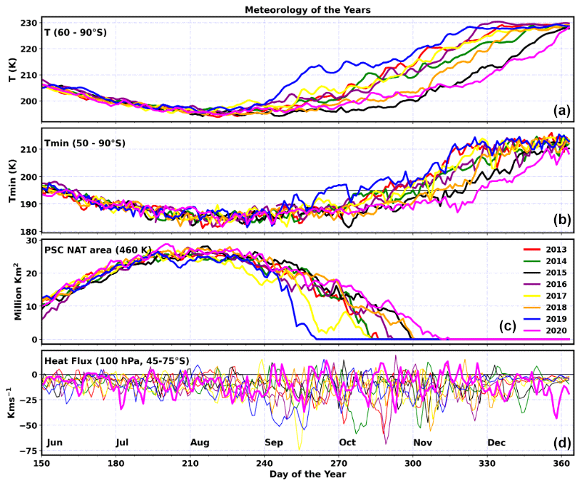
Figure 1 Meteorology of the years (2013–2020). Panel (a) shows the zonal average temperature (60–90° S) at 100 hPa. Panel (b) shows the minimum temperature at 100 hPa. The black horizontal line in the panels shows 195 K (PSC formation threshold). Panel (c) shows the PSC area at 460 K, and panel (d) shows the mean heat flux (45–75° S) at 100 hPa. The black horizontal line in panel (d) shows zero heat flux. NAT: nitric acid trihydrate.

Figure 1b shows the minimum polar cap temperature for each winter and is lower than the PSC formation threshold (195 K). This continues in the early spring for all years except 2019, and the minimum value rises soon after and is higher than 195 K in the late spring. The minimum temperature reaches this threshold for most days, and thus the ideal conditions for the formation of PSCs are found in all winters. Therefore, the PSC area has grown since the beginning of winter and is highest in August (up to 28×10⁶ km²). Corresponding to the periods of the longest duration of minimum temperature, PSCs persist until early November in 2015, 2018, and 2020 but are relatively short-lived in 2017 and 2019. As the mean temperature peaks in early to mid-September 2019, the PSC area drops and diminishes by late September. However, the PSCs dissipated by mid-October in 2017.

A major factor affecting the strength of polar vortex is tropospheric forcing. Strength of this forcing is very weak in the Antarctic, except for a few winters. According to Zuev and Savelieva (2019), the strengthening of the Antarctic polar vortex in winter and spring is due to the seasonal temperature variations in the subtropical lower stratosphere. Figure 1d shows the tropospheric forcing estimated for all years. The heat flux averaged between the adjacent mid-latitudes and higher latitudes is directed southward, particularly in the late winter and early spring. The years 2019 and 2017 are characterised by very strong wave forcing, as shown by the high flux values (from −40 to −50 km s⁻¹). Klekociuk et al. (2019) reported that the easterly phase of the quasi-biennial oscillation (QBO) favoured the enhanced wave activity in 2017, a reason for the relatively higher temperature in that winter. Milinevsky et al. (2020) and Evtushevsky et al. (2019) also found similar results for both winters. The zonal average of heat flux stays between −30 and 10 km s⁻¹ for most winters, and the flux increases as the spring approaches. However, these forcings are weak in the years 2015 and 2020.

3.2 Temporal evolution of temperature with altitude

Figure 2 shows the temporal evolution of zonal mean (60–90° S) temperature profiles in the Antarctic for the years 2013–2020. The coloured contours show the temperature across the seasons, and white contour lines represent 188, 195, and 210 K. Here, the zonal winds (westerlies) are overlaid with black contours, and the easterlies are in red. In general, temperature increases towards the end of spring in the stratosphere, but it started to rise in the lower stratosphere much earlier during the spring of 2019 and 2017. Temperature contours of 250–265 K extend to slightly below 10 hPa, and there is a small reduction in the speed of westerlies during the period. Temperatures below 195 K are found in the lower stratosphere (100–70 hPa) until mid-October in 2015 and 2020. Similarly, the area covered by < 195 K was also moderately large in 2013, 2014, 2016, and 2018. However, this is lowest in 2019 and relatively small in 2017. The appearance of easterlies below 10 hPa is late (end of November), and thus the vortex lasted longer in 2015 and 2020, whereas it is as early as late October in 2017 and 2019. We also made an assessment inside the vortex to examine the consistency of our analysis with and without the vortex criterion (see Fig. S1 in the Supplement). The key features are the same in both analyses, such as the very low temperatures in the lower stratosphere, strong westerlies and the late appearance of easterlies in the middle stratosphere in 2015 and 2020, the early appearance of easterlies and the minor warming in 2019, and the large and extended period of the PSC threshold temperature (195 K) in 2018. Since the meteorology is different inside the vortex, small differences in the temperature (e.g., PSC threshold area) and wind (middle-stratospheric westerlies in 2015 and 2020) values are also found between the two.

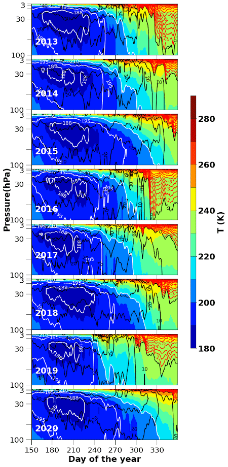
Figure 2 Seasonal march of the zonal mean temperature for the period 2003–2020 averaged over the latitudes 60–90° S. The contours show the temperature, and white contours represent specific temperatures such as 188, 195, and 210 K. The zonal wind velocities are overlaid. The black contour lines show the westerlies, and the red contour lines show the easterlies.

3.3 Ozone, chlorine activation, and ozone loss

Figure 3 shows the temporal evolution of ozone (in ppmv) inside the vortex deduced from the MLS data for the period 2013–2020. The ozone is lost in the lower altitudes as time progresses in spring, as illustrated in Fig. 3. It is observed from previous studies that the ozone loss is the maximum in the lower stratosphere in all years (Solomon, 1999). Contrary to this, ozone increases in the upper stratosphere as the winter progresses towards spring. Ozone in the lower stratosphere (400–600 K) is around 0.1–3 ppmv in 2013, 2014, 2015, 2016, 2018, and 2020. Unlike in the cold winters, ozone is slightly higher (by 0.5–1.5 ppmv) in the lowermost stratosphere in 2019. Similarly, in 2017, ozone in the lower stratosphere (400–450 K) is higher than that in the previous cold years, owing to the higher temperature there. The lowest ozone for the altitude range of 400–475 K is observed in 2015, 2018, and 2020, in which the 0.5 ppmv contour extends to 475–500 K.

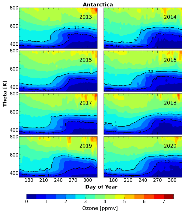
Figure 3 Temporal evolution of the vertical profiles of ozone averaged inside the vortex for the winters of 2013–2020 in the Antarctic. The temporal evolution is analysed using the MLS ozone data at 350–800 K for the period June–November. The black contours represent 1.0 and 2.5 ppm of ozone.

Figure 4 presents the temporal evolution of ClO (right) and ozone loss (left) at different altitudes during the period of study. Since there are unreasonably high tracer values in June due to the initialisation problem, the ozone loss is not calculated up to 10 June 2018 and 20 July 2019. In general, ozone loss is highest at 400–550 K (lower stratosphere) during September and October in all years. The loss is smaller than 1.4 ppmv in the upper stratosphere, mostly driven by the NO_x-based chemistry (e.g., Kuttippurath et al., 2015). The loss in 2014 and 2015 is almost similar, about 2.6–3.0 ppmv at the peak ozone loss altitude (450–550 K) during September and October. The loss in 2013 reaches up to 3.0 ppmv by mid-October and is higher than in 2014, 2015, 2017, and 2018 (e.g., Vargin et al., 2020). The ozone loss reported by Strahan and Douglass (2018) for 2015 is similar to the very cold winters in Antarctica and is slightly higher than our estimate for that winter. The ozone loss with altitude is larger in 2015 than the other winters (see Fig. 4). The preconditioning for ozone loss in 2013 and 2014 was ensured by high chlorine activation at the same altitude range (Kuttippurath et al., 2015). Among these 3 years (2013–2015), before the period of highest ozone loss, chlorine activation reaches its peak in August and September. ClO amounts to 2.2 ppbv in 2013 and 2014 and 2.0 ppbv in 2015 during this period. This high chlorine activation lasted for almost a month at the peak ozone loss altitudes (450–550 K) in 2013 but for a relatively shorter period in 2014 and 2015. Similar values for ozone loss and ClO (1.8–2.2 ppbv) are also estimated for 2017 and 2018, and the highest ClO value stayed intact for 15–20 d before attaining the maximum ozone loss.

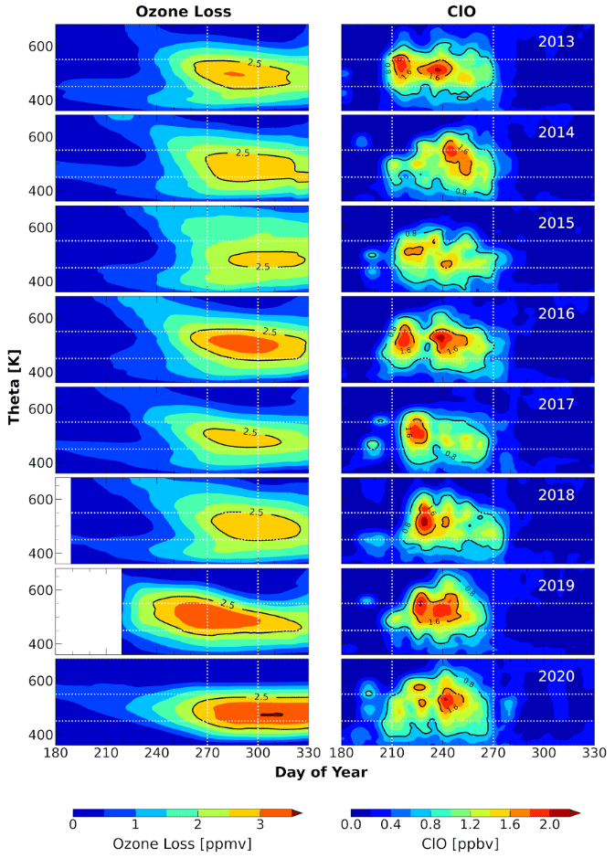
Figure 4 Temporal evolution of ozone loss estimated from MLS measurements using the REPROBUS passive tracer (left column). The MLS ClO measurements for the altitude range 350–700 K for the period 2013–2020 (right column). The ozone loss estimates and ClO measurements are selected inside the polar vortex as per the Nash et al. (1996) criterion. Ozone loss is not computed up to 10 June in 2018 and 20 July in 2019 because of the unavailability of tracer values. The black contours represent 2.5 and 3.5 ppm of ozone loss (left column) and 0.8 and 1.6 ppb of ClO (right column).

The ozone loss in 2016 is about 3–3.2 ppmv in September and 3.4 ppmv in October. Note that the ozone hole, PSC occurrence, and chlorine activation (more than a month, up to 2.2 ppbv) lasted longer in this year. An extensive ozone hole from late August to mid-November is found in 2019. However, ozone increased after the minor warming, and thus the ozone hole size (Fig. 3) and ozone loss reduced significantly thereafter (Fig. 4). The chlorine activation was very strong and continuous from August to September (above 2.2 ppbv) in this year. Despite the minor warming, the ozone loss in 2019 (3.0–3.4 ppmv) is similar to that in 2016. The nature of spring 2019 was similar to the previous warm Antarctic years of 1988 and 2002, as the vortex was short-lived and highly variable due to strong tropospheric forcing and SSW (Manney et al., 2020; Klekociuk et al., 2021). The peak ozone loss in 2019 is about 3.4 ppmv, which is higher than that in other winters, except 2020 (Wargan et al., 2020; Roy et al., 2022). The chlorine activation remained at its peak value (2.0–2.2 ppbv) for several days in August before reaching the peak ozone loss in 2019, and the spatial distribution (450–550 K) of these high ClO values is the largest compared to all other years. The 2020 ozone loss is very high (up to 3.6 ppmv) and exceeds the maximum ozone loss of other winters. The chlorine activation rose in the early spring (September) (2.0–2.2 ppbv) and is similar to that in 2016. The high values of ozone loss may have resulted from the increased aerosol loading from the Australian bushfires in 2020 (e.g., Stone et al., 2021). A recent study by Ansmann et al. (2022) shows that about ​​​​​​​10 %–20 % of the ozone loss in 2020 was driven by the wildfire smoke that caused the growth of PSC particles.

3.4 Interannual variability of ozone loss

The interannual variability of ozone loss, PSCs, and chlorine activation is shown in Fig. 5. Here, the ozone loss is computed by taking the average of ozone loss from day 270 to 300 (the peak loss period) in the altitude range 450–550 K (the peak loss altitudes; see Fig. 4). Similarly, the chlorine activation is indicated as the average of ClO over the same altitude range but for the days between 210 and 270 (peak chlorine activation period). The weighted mean of the PSC area is shown with a solid black line for the years 2013–2020. Note that the peak ozone loss duration and altitude range are different in different winters (e.g. 2018 and 2020). The smallest ozone loss is estimated for the years 2015 and 2017 because of relatively weak chlorine activation in those winters. The mean ozone loss is about 2.4 ppmv, and ClO is about 1.75–1.95 ppbv in both years. However, the PSC area in 2015 (11.9×10⁶ km²) was higher than most of the other cold winters. The larger PSC area is mostly because of the lower temperature conditions that lasted longer in the winter. Tully et al. (2019) identified 2015 as one of the most severe and extreme winters, as also observed in our study. The PSC area in 2017 (10.2×10⁶ km²) is smaller, and, therefore, ozone loss is lower as compared to that in 2015, which is consistent with the results of Braathen (2018).

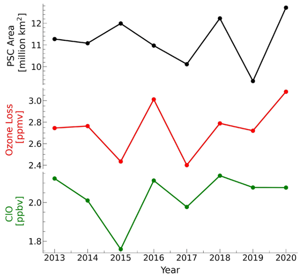
Figure 5 The vortex-averaged ozone loss estimated from the MLS measurements using the passive method, peak ClO measurements, and the weighted average of the PSC area for the period 2013–2020. The mean ozone loss is estimated over the altitude range 450–550 K and between day 270 and 300 (maximum ozone loss days). The ClO measurements are averaged over the altitude range 450–550 K and between day 210 and 270, representing the strong chlorine activation period and altitudes.

The highest ozone loss is estimated in 2020 (3.1 ppmv) in the spring, which is followed by 2016 (3.0 ppmv). The chlorine activation for both years is also higher than that of a few other cold winters, as shown by the ClO values of about 2.1–2.2 ppbv. The highest ozone loss in 2020 is favoured by the very large PSC area (12.6×10⁶ km²). The 2018 spring was also unique in comparison to the other years as a consequence of the high chlorine activation (2.2 ppbv) and very large PSC area (12.0×10⁶ km²). The chlorine activation was very high in 2019 (2.1 ppbv), but the relatively lower ozone loss during this particular period is a direct consequence of its unfavourable dynamic condition (SSW). The PSC area is also lowest in 2019 (9.4×10⁶ km²) among the winters due to SSW. The ozone loss (2.7–2.8 ppmv) and chlorine activation (2.1–2.2 ppbv) are similar in other winters.

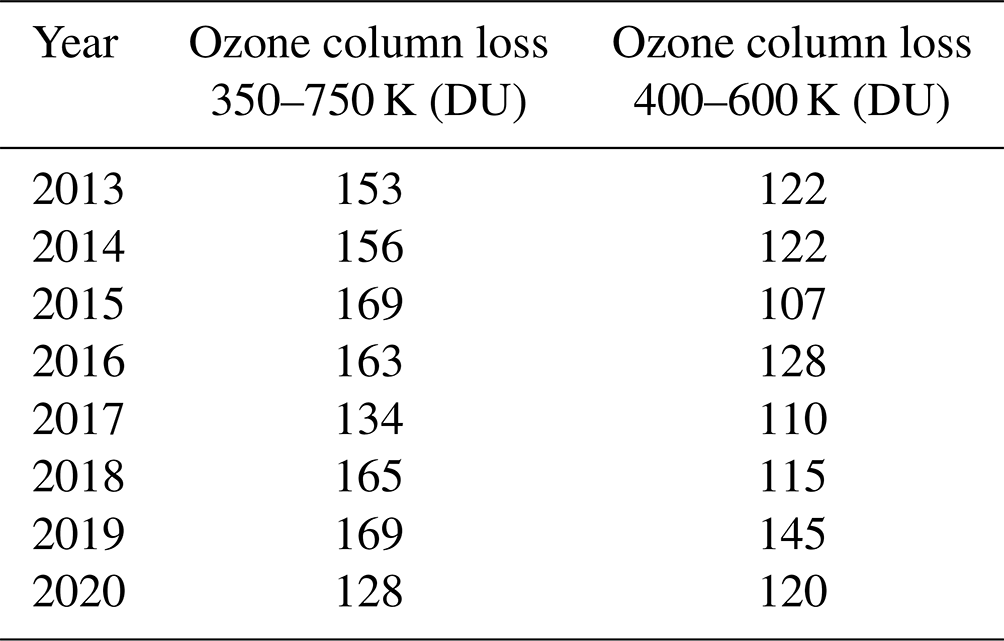
Table 1 shows the partial column ozone loss estimated with the MLS data and REPROBUS passive ozone simulations for two different altitude ranges. The partial column loss at 350–750 K yields similar values for most winters, as the highest loss is estimated for 2015, 2016, 2018, and 2019 (around 163 ± 16 DU), consistent with the meteorology of the winters. However, the lowest column loss (128 ± 12 DU, Dobson unit) is estimated for the winter of 2020, as the vertical spread of ozone loss is limited beyond the peak ozone loss altitude range of 450–550 K in this winter (see Fig. 4). Similarly, ozone loss in the moderately cold winters shows a loss of about 154 ± 15 DU (2013 and 2014) but very small loss in 2017 (134 ± 13 DU). The column loss computed at 400–600 K, the highest ozone loss altitudes in the Antarctic, has slightly lower values, as expected. In general, there is an average difference of about 40 DU of ozone loss (higher than the 400–600 K) between these altitude ranges (e.g., Kuttippurath et al., 2015). The loss is highest in 2019 (145 ± 14 DU) at 400–600 K as in the case of 350–750 K but smallest in 2015 (107 ± 10 DU). This suggests that there is higher ozone loss at altitudes above 600 K in the very cold winter of 2015 (see Fig. 4). On the other hand, ozone loss and its difference between these two altitude ranges are very small for 2020 and 2017, as discussed before.

Table 1 The partial column ozone loss computed using the MLS ozone measurements and modelled tracer by applying the passive method. The column loss is estimated for the peak ozone altitude ranges of 350–750 and 400–600 K. The ozone column loss estimates have an uncertainty of about 10 %.

4 Conclusions

We analyse the ozone loss for the past 8 years (2013–2020) in the Antarctic. The year 2019 had a warm winter with a mW in mid-September. The winter of 2017 also shows similar characteristics, such as the sudden increase in temperature during late August, the higher minimum temperature (about 205 K) in August than in other years, and the sharp decrease in the PSC area towards the end of September. The heat flux magnitude for the year (2017) is also higher than that in other winters (up to −60 km s⁻¹), suggesting that it was a disturbed warm winter. We find a minimal ozone loss in 2017, and it stayed less than 2.8 ppmv (110 ± 11 DU at 400–600 K) for most of October and September. Chlorine activation was also below 1.8 ppbv during August and September in the year. Conversely, the wave fluxes are lowest in 2015. The temperature and PSC area follow similar temporal evolution in 2013, 2014, 2015, 2016, and 2018. Winter 2020 exhibits unique meteorology with a long-lasting occurrence of vortex-wide PSCs (12.6×10⁶ km²) and thus shows the highest ozone loss (3.5 ppmv). On the other hand, the lowest ozone loss (2.5 ppmv or 107 ± 10 DU at 400–600 K) is estimated in 2015. Our study thus helps in understanding how the chlorine activation and meteorology of the winters influence the variability of ozone. Dynamics and chemistry of the winters play their respective roles in the ozone loss process. The winter of 2019 is an example of favourable chemistry helping in the large loss in ozone, though the dynamical conditions were unfavourable.