Bias correction of OMI HCHO columns based on FTIR and aircraft measurements and impact on top-down emission estimates

Spaceborne formaldehyde (HCHO) measurements constitute an excellent proxy for the sources of non-methane volatile organic compounds (NMVOCs). Past studies suggested substantial overestimations of NMVOC emissions in state-of-the-art inventories over major source regions. Here, the QA4ECV (Quality Assurance for Essential Climate Variables) retrieval of HCHO columns from OMI (Ozone Monitoring Instrument) is evaluated against (1) FTIR (Fourier-transform infrared) column observations at 26 stations worldwide and (2) aircraft in situ HCHO concentration measurements from campaigns conducted over the USA during 2012–2013. Both validation exercises show that OMI underestimates high columns and overestimates low columns. The linear regression of OMI and aircraft-based columns gives ${\mathrm{\Omega }}_{\mathrm{OMI}}=\mathrm{0.651}{\mathrm{\Omega }}_{\mathrm{airc}}+\mathrm{2.95}\times {\mathrm{10}}^{\mathrm{15}}$ ${\mathrm{molec}.\mathrm{cm}}^{-\mathrm{2}}$, with Ω_OMI and Ω_airc the OMI and aircraft-derived vertical columns, whereas the regression of OMI and FTIR data gives ${\mathrm{\Omega }}_{\mathrm{OMI}}=\mathrm{0.659}{\mathrm{\Omega }}_{\mathrm{FTIR}}+\mathrm{2.02}\times {\mathrm{10}}^{\mathrm{15}}$ ${\mathrm{molec}.\mathrm{cm}}^{-\mathrm{2}}$. Inverse modelling of NMVOC emissions with a global model based on OMI columns corrected for biases based on those relationships leads to much-improved agreement against FTIR data and HCHO concentrations from 11 aircraft campaigns. The optimized global isoprene emissions ($\sim \mathrm{445}{\mathrm{Tg}\mathrm{yr}}^{-\mathrm{1}}$) are 25 % higher than those obtained without bias correction. The optimized isoprene emissions bear both striking similarities and differences with recently published emissions based on spaceborne isoprene columns from the CrIS (Cross-track Infrared Sounder) sensor. Although the interannual variability of OMI HCHO columns is well understood over regions where biogenic emissions are dominant, and the HCHO trends over China and India clearly reflect anthropogenic emission changes, the observed HCHO decline over the southeastern USA remains imperfectly elucidated.

1 Introduction

The atmospheric oxidation of non-methane volatile organic compounds exerts multiple influences on tropospheric ozone (e.g., Chameides et al., 1988; Archibald et al., 2020), fine particulate matter (e.g.,  Spracklen et al., 2011; Miao et al., 2021) and the oxidizing capacity of the atmosphere (e.g., Seinfeld and Pandis, 1988; Martinez et al., 2003; Bates and Jacob, 2019). Quantifying those impacts is made difficult by the large number and diversity of non-methane volatile organic compounds (NMVOCs), with chemical lifetimes ranging from a few minutes to several months (Shu and Atkinson, 1994; Atkinson, 2000), and by important gaps in our understanding of their emissions and chemical degradation mechanisms. Even biogenic isoprene, the most abundantly emitted NMVOC at the global scale, has very uncertain emissions due (among others) to the strong variability of emission rates among different plant species (Guenther et al., 2006) and to the large uncertainties in the climate and vegetation maps used to calculate the fluxes in state-of-the-art emission models (Arneth et al., 2011; Sindelarova et al., 2014). In addition, field campaigns in various environments such as cities (e.g., Karl et al., 2018) and remote areas (e.g., Read et al., 2012; Wang et al., 2012; Lawson et al., 2015; Travis et al., 2020) suggest that current inventories of anthropogenic and natural emissions of many NMVOCs and particularly oxygenated volatile organic compounds (OVOCs) are incomplete. The comparison of measured total OH reactivity with the sum of contributions from measured individual compounds over forests has revealed the presence of a “missing OH reactivity” that is partly, but not always completely, explained by unobserved oxidation products of known VOC precursors (Di Carlo et al., 2004; Sinha et al., 2010; Yang et al., 2016; Nölscher et al., 2016; Sanchez et al., 2021), thereby providing additional indication that primary emissions are missed in emission inventories. For biomass burning as well, the contribution of unidentified organic compounds to the total NMVOC fluxes might be of the same order or even larger than the explicitly identified compounds (Akagi et al., 2011; Andreae, 2019).

Since chemical transport models (CTMs) do not include unidentified NMVOCs, they are expected to underestimate the total NMVOC flux. Nevertheless, CTMs using state-of-the-art emission inventories (Guenther et al., 1995, 2006) were found to overestimate the column abundances of formaldehyde, a major NMVOC oxidation product, against retrieved columns from spaceborne UV–visible sounders such as the Scanning Imaging Absorption Spectrometer for Atmospheric Chartography/Chemistry (SCIAMACHY;  Stavrakou et al., 2009; Barkley et al., 2011) and the Ozone Monitoring Instrument (OMI;  Millet et al., 2008; Barkley et al., 2011; Fortems-Cheiney et al., 2012; Stavrakou et al., 2015; Bauwens et al., 2016). Furthermore, the largest model biases (exceeding −40 %) were found over high-emission areas such as Amazonia, the central African rainforest and the southeastern USA (Barkley et al., 2011; Marais et al., 2014; Bauwens et al., 2016), where isoprene oxidation is believed to be by far the largest source of formaldehyde (Palmer et al., 2003; Stavrakou et al., 2009). Note that earlier studies using HCHO retrievals from the pioneering Global Ozone Monitoring Experiment (GOME;  Palmer et al., 2003, 2006; Abbot et al., 2003; Shim et al., 2005; Fu et al., 2007; Stavrakou et al., 2009) led to mixed conclusions with both model underestimations and overestimations, primarily due to large differences between different retrievals (De Smedt et al., 2008; Stavrakou et al., 2009). We restrict the following discussion to studies based on subsequent, higher-resolution sounders, in particular OMI.

The general model overestimation of spaceborne HCHO abundances over source regions was mainly attributed to an overestimation of isoprene emissions estimated using the Model of Emissions of Gases and Aerosols from Nature (MEGAN;  Guenther et al., 2006, 2012), and inverse modelling of emissions – i.e., the derivation of improved emissions constrained by observational data while accounting for the error covariances of the data and the a priori emissions – has led to a reduction of biogenic emissions globally (e.g.,  Bauwens et al., 2016). The overestimation of isoprene emissions was also concluded in several studies based on model comparisons with isoprene concentration measurements, in particular over tropical ecosystems (e.g.,  Houweling et al., 1998; Bey et al., 2001). However, those comparisons are uncertain, due (among others) to the strong variability of isoprene concentrations and to their dependence on OH radical levels, likely too low in those models due to the neglect of OH-recycling mechanisms which were not yet identified (Lelieveld et al., 2008; Paulot et al., 2009; Peeters et al., 2014; Wennberg et al., 2018; Novelli et al., 2020). A more recent evaluation indicates a model underestimation against aircraft measurements of many reactive VOCs, including formaldehyde and isoprene, over North America (Chen et al., 2019). In addition, recent isoprene flux measurements by eddy covariance from airborne platforms did not suggest overestimations of MEGAN-calculated emissions over the Amazon forest (Gu et al., 2017), the southeastern USA (Yu et al., 2017) or California (Misztal et al., 2014).

Whereas validation studies of the Harvard GOME retrieval showed a good consistency of spaceborne columns against aircraft in situ observations (Martin et al., 2004; Millet et al., 2006), evaluation of OMI HCHO columns against three aircraft campaigns (Boeke et al., 2011) also indicated a good agreement (−3 % bias) with respect to the mean aircraft-based columns but displayed a larger relative bias (−17 %) for higher columns ($>\mathrm{5}\times {\mathrm{10}}^{\mathrm{15}}{\mathrm{molec}.\mathrm{cm}}^{-\mathrm{2}}$). The latter was tentatively attributed to the preferential sampling of polluted plumes by the aircraft, since the highest HCHO columns were measured in the vicinity of Mexico City and an airshed near Houston, Texas. However, similar or even larger biases were found in the comparison of HCHO columns from several spaceborne sensors, including OMI, against in situ measurements of the SEAC⁴RS campaign conducted over a wide area covering much of the southeastern USA during summer, a region with high HCHO abundances of primarily biogenic origin (Zhu et al., 2016). The lowest bias (−20 %) was realized by the OMI BIRA-V14 retrieval (De Smedt et al., 2015) and could be further reduced (to −12 %) when adopting the aircraft vertical shape profiles in the calculation of air mass factors of the OMI retrieval.

The first evaluations of HCHO satellite columns using Fourier-transform infrared (FTIR) measurements were conducted in remote environments (Jones et al., 2009; Vigouroux et al., 2009) and suggested a fairly good agreement. In contrast with this and in qualitative agreement with the results of Boeke et al. (2011), the recent evaluation of TROPOMI (TROPOspheric Monitoring Instrument) HCHO columns against FTIR measurements from a network of 25 stations worldwide showed a pronounced dependence of the bias of TROPOMI columns with the column magnitude, with overestimations (averaging +25 %) found for very low columns ($<\mathrm{2.5}\times {\mathrm{10}}^{\mathrm{15}}{\mathrm{molec}.\mathrm{cm}}^{-\mathrm{2}}$) and underestimations (−30.8 %) for high columns ($>\mathrm{8}\times {\mathrm{10}}^{\mathrm{15}}{\mathrm{molec}.\mathrm{cm}}^{-\mathrm{2}}$). The largest underestimation (−36 %) was found for the station with the highest average HCHO column, i.e., Porto Velho in Amazonia ($\mathrm{29}\times {\mathrm{10}}^{\mathrm{15}}{\mathrm{molec}.\mathrm{cm}}^{-\mathrm{2}}$). Comparable biases can be expected for OMI as for TROPOMI, given the similarity between the two instruments (De Smedt et al., 2021).

Acknowledging the potentially important consequences of such biases on top-down VOC emission estimates based on spaceborne HCHO columns, we aim (1) to assess the biases of HCHO columns from a recent OMI retrieval (De Smedt et al., 2018) using both FTIR data (using a methodology similar to Vigouroux et al., 2020) and in situ aircraft measurements from several campaigns in the USA and (2) to investigate the consequences of those biases for inverse modelling of NMVOC emissions based on OMI data.

The paper is structured as follows. Section 2 describes the OMI retrieval, the network of FTIR data and the airborne datasets used in this work; Sect. 3 presents the validation methodology, the model setup and the emission inversions; Sect. 4 presents the correction of OMI biases using FTIR and aircraft data and proposes a bias-correction formula for use in inverse modelling; Sect. 5 presents an assessment of top-down VOC emissions based on OMI, with and without bias correction; it also provides an evaluation of the optimized results against independent data,and examines the long-term variability and trends of VOC emissions based on the OMI dataset between 2005 and 2016; finally, Sect. 6 presents the conclusions of this study.

2 Description of observational datasets

2.1 The OMI HCHO columns

The Ozone Monitoring Instrument (OMI) was launched in 2004 aboard the Aura satellite in a low Earth polar orbit crossing the Equator around 13:30 LT (local time). OMI is a nadir spectrometer that measures the solar radiation backscattered by the Earth's atmosphere and surface between 270 and 500 nm (Levelt et al., 2006). OMI has a 2600 km wide swath (divided into 60 across-track rows), providing near-global coverage every day. Due to an anomaly affecting the CCD detector, an increasing number of rows had to be filtered out, resulting in gradual degradation of the coverage to about 50 % (Torres et al., 2018). The OMI ground pixel size varies from 13×24  km² at nadir to 28×150  km² at the edges of the swath.

The OMI HCHO dataset (v1.2, https://doi.org/10.18758/71021031) was developed within the QA4ECV project of the Seventh Framework Programme of the European Union (EU-FP7). The retrieval algorithm for HCHO is described in De Smedt et al. (2018). It is based on a three-step DOAS (differential optical absorption spectroscopy) method. First, the fit of the slant columns is performed in a spectral window between 328.5 and 359 nm, with HCHO cross sections from Meller and Moortgat (2000). The slit function of each OMI row is adjusted on a daily basis as part of the wavelength calibration procedure, and the absorption cross sections are convolved accordingly. The DOAS reference spectrum is updated every day with averaged Earth radiances measured in the equatorial Pacific. The fit therefore provides a differential slant column, which corresponds to the HCHO excess over source regions in comparison to the remote background. In a second step, the slant columns are converted to tropospheric vertical columns using a lookup table of vertically resolved air mass factors calculated at 340 nm using the VLIDORT v2.6 radiative transfer model (Spurr, 2008). Surface albedo is obtained from the monthly OMI climatology at 0.5^∘ resolution (Kleipool et al., 2008). Daily a priori vertical profiles are obtained from the TM5 analysis, at 1^∘ spatial resolution (Williams et al., 2017). The standard air mass factor (AMF) calculations use the effective cloud fraction and cloud-top pressure from the Fresco v7 cloud product (Veefkind et al., 2016), treating clouds as Lambertian reflectors and applying the independent pixel approximation (Martin et al., 2002; Boersma et al., 2004). However, in this work, the cloud correction to the AMF calculation is switched off, except for a strict filtering (effective cloud fraction > 0.2). Clear-sky AMFs are used in lieu of the cloud-corrected AMFs. This choice ensures an optimal consistency with the TROPOMI HCHO dataset (De Smedt et al., 2021). Indeed, the TROPOMI HCHO retrieval is inherited from the QA4ECV algorithm with the aim to generate a consistent time series of early afternoon observations. Finally, to correct for any global offset and for stripes arising between the rows, a background correction is applied on a daily basis using the HCHO slant columns over the Pacific Ocean. The TM5 HCHO model columns derived in the same region are finally added to the vertical columns to compensate for the background HCHO concentrations. Several diagnostic variables are provided together with the measurements. Besides the cloud filter, the recommended processing is applied, in particular with respect to the row anomaly (De Smedt et al., 2018). For every pixel, column averaging kernels and a priori profiles are provided, as well as the random and systematic components of the tropospheric column uncertainty.

2.2 Ground-based FTIR HCHO data

The FTIR stations participating in the present study are listed in Table S1 in the Supplement (see also Fig. 1b). Most stations are affiliated to the Network for the Detection of Atmospheric Composition Change (NDACC) (De Mazière, 2018). The InfraRed Working Group (IRWG) of NDACC (https://www2.acom.ucar.edu/irwg, last access: 19 February 2024) requires standardized high-quality instruments, namely, high-resolution spectrometers mostly from the same manufacturer (Bruker 120HR or 125HR), and homogenized retrieval algorithms: PROFITT9 (Hase et al., 2006) and SFIT4 (Pougatchev et al., 1995). These codes retrieve information on atmospheric composition from solar absorption measurements performed under clear-sky conditions in the infrared spectral region and provide total columns as well as low-vertical-resolution profiles of many atmospheric species.

Harmonized retrieval settings have been set up and used within the whole IRWG in order to build a consistent ground-based FTIR HCHO dataset for robust interpretation of satellite and model validation (Vigouroux et al., 2018). This dataset has proven its value for the validation of TROPOMI HCHO (Vigouroux et al., 2020, see also the quarterly reports https://mpc-vdaf.tropomi.eu, last access: 19 February 2024), of GOME-2 (https://acsaf.org/valreps.php, last access: 19 February 2024) or more recently of OMPS (Kwon et al., 2023). We refer to Vigouroux et al. (2018) for details about the HCHO retrieval settings. The most critical aspects with regard to harmonization within the network are the spectral signatures and the spectroscopic parameters. The HCHO fitted spectral signatures belong to the ν₁ and ν₅ vibrational bands, around 3.6 µm. The spectroscopic database is the atm16 line list from G. Toon (http://mark4sun.jpl.nasa.gov/toon/linelist/linelist.html, last access: 19 February 2024), which corresponds to HITRAN 2012 (Rothman et al., 2013) for formaldehyde. Low-vertical-resolution formaldehyde profiles are obtained using Tikhonov regularization (Tikhonov, 1963). However, the degrees of freedom for signal (DOFS) are low for HCHO (from 1 to 1.6) due to its weak spectral signature, implying that mainly a total column can be retrieved. The sensitivity of the measurement is highest in the free troposphere, but a good sensitivity is achieved near the surface (see Fig. 4 of Vigouroux et al., 2018). The FTIR HCHO uncertainty is calculated according to Rodgers (2000). The systematic uncertainty, mostly due to uncertainty on the spectroscopic parameters, is ∼13 % (Vigouroux et al., 2018). The random uncertainties can be as low as $\mathrm{1.0}\times {\mathrm{10}}^{\mathrm{14}}{\mathrm{molec}.\mathrm{cm}}^{-\mathrm{2}}$ (8 %) for clean sites such as Eureka and up to $\mathrm{5.3}\times {\mathrm{10}}^{\mathrm{14}}{\mathrm{molec}.\mathrm{cm}}^{-\mathrm{2}}$ (7 %) for polluted stations such as Paris. Only the Mexico City site has a larger random uncertainty ($\mathrm{11.1}\times {\mathrm{10}}^{\mathrm{14}}{\mathrm{molec}.\mathrm{cm}}^{-\mathrm{2}}$) because it operates a low-resolution spectrometer (Vertex 80). Additionally, note that significant random and systematic smoothing uncertainties also exist (Vigouroux et al., 2018); however, those uncertainties vanish when the FTIR averaging kernels are used to smooth the model profiles, as done in this study (Rodgers and Connor, 2003).

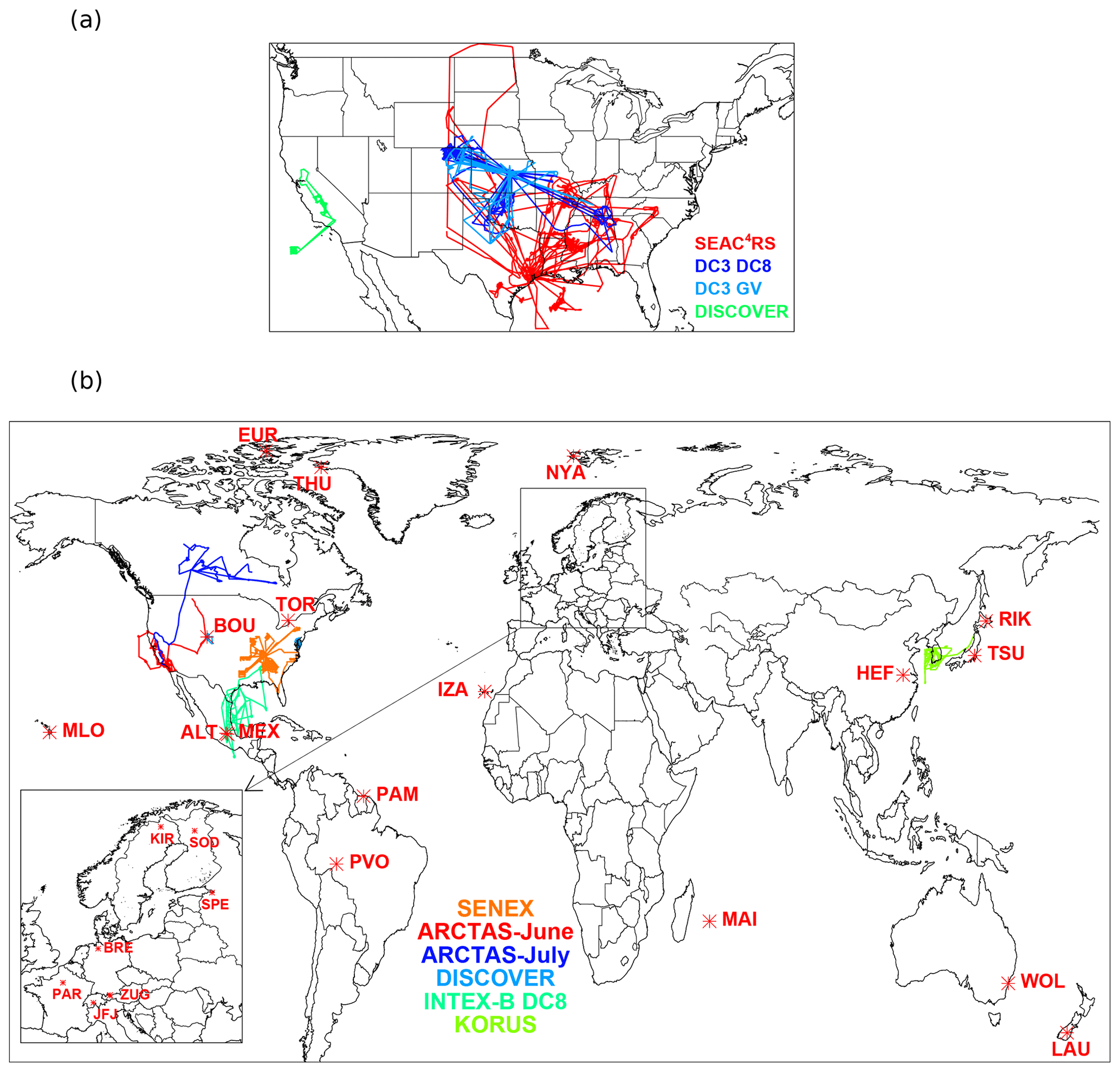
Figure 1 (a) Flight tracks of the aircraft missions (DC3, SEAC⁴RS, DISCOVER-AQ California) used as constraints in the aircraft-based inversion; (b) flight tracks of the additional aircraft campaigns used for global model evaluation and location of FTIR stations used in this work to evaluate OMI HCHO columns. The station coordinates and codes are provided in Table S1. Note that the stations Garmisch and Saint-Denis are not shown, given their close proximity to the stations Zugspitze (ZUG) and Maïdo (MAI), respectively.

2.3 Airborne HCHO data

Table 1 lists the aircraft campaign data used in this study. Among those, four HCHO datasets from three campaigns conducted during 2012–2013 over the United States are used to evaluate OMI HCHO columns, as described in Sect. 3.3. Those campaigns, as well as seven additional campaigns (datasets 5–11 in Table 1), are used to evaluate the inverse modelling results. More specifically, the following campaigns are explained.

• The DC3 (Deep Convective Clouds and Chemistry) NASA mission sampled the atmospheric composition over the central USA during May–June 2012 (Barth et al., 2015). Formaldehyde mixing ratios were acquired from two aircraft platforms, the NASA DC-8 and the NSF/NCAR Gulfstream V (GV), equipped with similar infrared absorption spectrometers employing difference frequency generation (DFG) laser sources: the DFGAS (difference frequency generation absorption spectrometer) instrument on the DC-8 (Weibring et al., 2007) and the more sensitive CAMS (compact atmospheric multispecies spectrometer) instrument on the GV (Richter et al., 2015). More details regarding the instruments can be found in Fried et al. (2016). A comparison between the DFGAS and CAMS measurements indicates a very good agreement between the two instruments, with the DFGAS measurements being slightly higher (by 11 %, Fried et al., 2016).

• The SEAC⁴RS (Studies of Emissions, Atmospheric Composition, Clouds and Climate Coupling by Regional Surveys) campaign was conducted over the southeastern USA in August–September 2013 on board the NASA DC-8 aircraft (Toon et al., 2016). The mission took place over regions rich in biogenic VOC emissions. Two different instruments were used: CAMS and the ISAF (in situ airborne formaldehyde) instrument (Cazorla et al., 2015). The ISAF data were found to be about 10 % higher than the CAMS values (Zhu et al., 2016). Only the CAMS data are used here.

• DISCOVER-AQ (Deriving Information on Surface conditions from Column and Vertically Resolved Observations Relevant to Air Quality) was a multi-year aircraft mission led by NASA (Crawford and Pickering, 2014). The HCHO measurements were acquired using the DFGAS technique (Weibring et al., 2007). The campaign over California (January–February 2013) is used in the OMI HCHO validation. The campaigns over Maryland (2011) and Colorado (2014) are used for model evaluation.

• The INTEX (Intercontinental Chemical Transport Experiment) campaigns took place in 2004 and 2006. We use here the measurements of the March 2006 INTEX-B campaign, also named MILAGRO (Megacity Initiative: Local and Global Research Observations) (Molina et al., 2010). The NASA DC-8 measured the chemical composition over Mexico, Texas and the Gulf of Mexico below ca. 10 km altitude. HCHO was measured using tunable diode laser spectroscopy (TDLAS) (Fried et al., 2008). The INTEX-B campaign of April–May 2006 is not used here, as it was conducted primarily over the Pacific Ocean, where HCHO levels are insensitive to emissions over land.

• The ARCTAS (Arctic Research of the Composition of the Troposphere from Aircraft and Satellites) campaigns took place in 2008 (Jacob et al., 2010). Whereas the ARCTAS-A campaign (not used here) targeted the springtime atmospheric composition over the Arctic, the ARCTAS-CARB (June) and ARCTAS-B (July) campaigns sampled the tropospheric composition during the summer between 34 and > 80^∘ N. Only data below 60^∘ N are used here. The TDLAS technique (see above) was employed to measure HCHO during both missions.

• The Southeast Nexus (SENEX) campaign (Warneke et al., 2016) used the NOAA WP-3D aircraft to sample the lower troposphere (below ca. 6 km altitude) over the southeast USA in June 2013. HCHO was measured using the ISAF instrument (see above).

• The KORUS-AQ (Korea-United States Air quality) campaign investigated air composition over Korea and surrounding areas in May–June 2016. Formaldehyde was measured throughout the troposphere by the NASA DC-8 using CAMS (see above).

Weibring et al. (2007)Richter et al. (2015)Richter et al. (2015)Weibring et al. (2007)Fried et al. (2008, 2011)Fried et al. (2008)Fried et al. (2008)Weibring et al. (2007)Weibring et al. (2007)Cazorla et al. (2015)Richter et al. (2015)Fried et al. (2020)

Table 1 Aircraft campaign datasets used in this work for OMI and model evaluation. Datasets 1–4 are used to determine the OMI biases. All datasets are used to evaluate the top-down emission inversions.

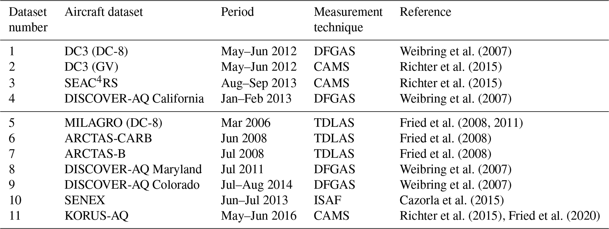
For all campaigns, we exclude HCHO measurements from urban plumes (identified as [NO₂]>4 ppbv or [NO_x]/[NO_y]>0.4) and biomass burning plumes ([CH₃CN]>225 pptv), as well as nighttime data (before 09:00 or after 18:00 LT, local time) and measurements over oceans. Data above 4 km altitude are also excluded. Furthermore, as the average HCHO mixing ratio from the CAMS instrument was about 13 % lower than those of the ISAF instrument during SEAC⁴RS, we increase the CAMS values by 6.5 % in order to bring the SEAC⁴RS data midway between CAMS and ISAF, while also reducing the bias between the GV data (CAMS) and DC-8 data (DFGAS) from the DC3 mission.

The measurements are publicly available via data archive centers (see “Data availability” section). The flight tracks are shown in Fig. 1.

2.4 Spaceborne isoprene columns from CrIS

The global modelling results of Sect. 5 will be evaluated against emissions derived from spaceborne isoprene column measurements (Sect. 5.3). The first global isoprene observations from space were derived through the application of an efficient machine-learning algorithm to thermal infrared radiances measured by the Cross-track Infrared Sounder (CrIS) (Wells et al., 2020). Isoprene column abundances were derived from on-peak/off-peak brightness temperature differences at the ν₂₈ absorption feature. Isoprene emissions for 3 months (January, April and July 2013) were derived from the CrIS measurements and the GEOS-Chem chemical transport model through the application of an iterative mass balance algorithm. Prior to the inversion of isoprene fluxes, NO_x fluxes were inverted using spaceborne NO₂ column data from the OMI sounder. This NO_x adjustment was found to be critical due to the high sensitivity of isoprene columns to OH (and hence NO_x) fields in the model. The isoprene inversion pinpointed several regions where emission errors for both isoprene and NO_x cause major prediction biases in models.

3 Methodology

3.1 Validation using FTIR measurements

The validation of OMI HCHO data using the FTIR ground-based network follows the methodology applied for TROPOMI by Vigouroux et al. (2020). Only the co-location criteria are chosen differently, due to the lower precision of OMI compared to TROPOMI columns: we average the OMI pixels within 50 km around each station, which leads to a mean value of 13 pixels per co-location. Only pixels satisfying the recommended quality criteria (Sect. 2.1) are averaged. In addition, the co-located pair is kept only if at least 10 valid OMI pixels are available for averaging.

We apply the formalism of Rodgers and Connor (2003) in order to account for the different a priori vertical profiles in the FTIR and OMI retrievals (single climatological profile from the WACCM model and daily profiles from TM5, respectively) and for the different vertical sensitivities of both instruments. For each FTIR profile in time coincidence (within 3 h of the OMI overpass time) and for each individual OMI pixel (within 50 km of the station), the OMI a priori profile is substituted for the FTIR profile (see Eq. 2 in  Vigouroux et al., 2020), and the corrected FTIR profile is smoothed after regridding (and extrapolation if needed) to the satellite grid using the OMI averaging kernel (Eq. 3 of  Vigouroux et al., 2020). The vertical regridding ensures that the same upper boundary for the tropospheric column definition is used in both products (the one from OMI). In addition, a scaling factor is applied to the OMI and smoothed FTIR columns to correct for the altitude difference between the OMI pixel and the station (Eq. 4 of  Vigouroux et al., 2020). That factor is taken as the fraction of the a priori OMI column that lies above the station altitude.

In summary, each coincident pair consists of the average of the smoothed and scaled FTIR columns within 3 h of the OMI overpass and the average of the individually scaled OMI pixels within 50 km of the station.

3.2 HCHO simulation using the MAGRITTEv1.1 CTM

The Model of Atmospheric composition at Global and Regional scales using Inversion Techniques for Trace gas Emissions (MAGRITTE v1.1) is a chemical transport model based on the previous IMAGES (Intermediate Model for the Annual and Global Evolution of Species) model (Muller and Brasseur, 1995; Stavrakou et al., 2018). MAGRITTE v1.1 calculates the distribution of 182 chemical species, among which 141 compounds undergo transport (advection, deep convection and turbulent mixing in the boundary layer) in the model. The chemical mechanism includes a detailed description of isoprene and other biogenic volatile organic compound (BVOC) oxidation mechanisms (Müller et al., 2019). In particular, it incorporates an up-to-date representation of isoprene peroxy radical unimolecular reactions and other recent mechanistic advances relevant to BVOC oxidation (Müller et al., 2019). The photolysis rates are interpolated from tabulated values calculated using the TUV photolysis estimation package (Madronich and Flocke, 1998). Most model parameterizations, including the chemical mechanism for anthropogenic and pyrogenic organic compounds, are obtained from the IMAGES model (Stavrakou et al., 2009; Bauwens et al., 2016). MAGRITTE can be run either as a global model, at 2^∘ × 2.5^∘ resolution, or as regional model, at 0.5^∘ × 0.5^∘ resolution. In regional mode, the boundary conditions of the lateral borders are provided offline by the global model. The chemical concentrations are calculated on a sigma–pressure coordinate grid, with 40 vertical levels distributed within the troposphere and the lower stratosphere (below the 44 hPa level).

Meteorological fields are obtained from the ERA5 ECMWF reanalysis (Hesbach et al., 2020). The effect of diurnal variation on the photolysis rates and kinetic rate constants are taken into account through correction factors calculated from model simulations with a 20 min time step. These correction factors are used to calculate the diurnal cycle of HCHO columns required for the comparisons with ground-based and aircraft measurements.

Anthropogenic emissions of CO, NO_x, SO₂ and carbonaceous aerosols are taken from the HTAPv2 (Hemispheric Transport of Air Pollution version 2) inventory (Janssens-Maenhout et al., 2015) for 2010. The anthropogenic NO_x emissions over the USA are adjusted (Travis et al., 2016; Müller et al., 2019) to match observed NO_x concentration and HNO₃ deposition data. The speciated emissions of NMVOCs are obtained from the EDGARv4.3.2 inventory (Huang et al., 2017) between 2005 and 2012 and are taken to be equal to their 2012 values afterwards. The global annual anthropogenic NMVOC source is estimated at 162.3 Tg in 2005 and increases annually by >1 % to reach 179.8 Tg in 2012. Vegetation fire emissions are provided from the GFED4s database (van der Werf et al., 2017), with vertical injection profiles from Sofiev et al. (2013). The global biomass burning flux is estimated to range between 78 and 107 Tg yr⁻¹, and the average global flux over 2005–2017 was 90.5 Tg yr⁻¹. Isoprene and monoterpene fluxes are calculated by the MEGAN model embedded in the MOHYCAN canopy environment model (Müller et al., 2008; Guenther et al., 2012; Bauwens et al., 2018) at 0.5^∘ × 0.5^∘ based on the ERA5 reanalysis meteorological fields and leaf area index (LAI) data from MODIS Collection 6 reprocessed by Yuan et al. (2011). The CO₂ inhibition effect is accounted for using the parameterization of Possell and Hewitt (2011). The effects of soil moisture stress are neglected, since previous model evaluations against OMI data have shown a deterioration of temporal correlation when accounting for the soil moisture activity factor calculated using MEGANv2.1 (Guenther et al., 2006) and ECMWF soil moisture fields (Bauwens et al., 2018; Stavrakou et al., 2018). The global annual isoprene flux ranges between 414 Tg (in 2008) and 452 Tg (in 2016). The average annual flux amounts to 433 Tg yr⁻¹ over 2005–2017. Biogenic methanol is also calculated according to MEGAN as described in Stavrakou et al. (2011). The monthly fluxes of isoprene and methanol emissions are available online at http://emissions.aeronomie.be (last access: 19 February 2024). The annual monoterpene fluxes range between 109 Tg (in 2008) and 120 Tg (in 2016). Biogenic acetaldehyde and ethanol emissions (amounting to 22 Tg yr⁻¹ for each compound) are calculated as described in Millet et al. (2010). Biogenic emissions of C₂H₄ (scaled to 4 Tg yr⁻¹ globally), HCHO (4 Tg yr⁻¹) and CH₃COCH₃ (28 Tg yr⁻¹) are also obtained from MEGAN (Guenther et al., 2012) (http://eccad.aeris-data.fr, last access: 19 February 2024). Finally, oceanic emissions are included for acetaldehyde (56 Tg yr⁻¹), methanol (49 Tg yr⁻¹) and acetone (63 Tg yr⁻¹) (Müller et al., 2019).

3.3 Aircraft-based inversion

The regional MAGRITTE model with its inverse modelling capability is used to generate HCHO model distributions that closely approximate the aircraft observations from the campaigns DC3, SEAC⁴RS and DISCOVER-AQ California (Table 1). This is realized by adjusting the monthly NMVOC emissions used in the model and minimizing a cost function which quantifies the overall discrepancy between the model-calculated mixing ratios and the observations. The cost function (J) is expressed as

$$\begin{array}{}\text{(1)}& J\left(\mathit{f}\right)={\displaystyle \frac{\mathrm{1}}{\mathrm{2}}}\left[{\left(H\left(\mathit{f}\right)-\mathit{y}\right)}^T{\mathbf{E}}^{-\mathrm{1}}\left(H\left(\mathit{f}\right)-\mathit{y}\right)+{\mathit{f}}^T{\mathbf{B}}^{-\mathrm{1}}\mathit{f}\right],\end{array}$$

where f denotes the vector of dimensionless emission parameters, H(f) is the chemical transport model operating on the control variables, y is the observation vector, and E and B are the covariance matrices of the errors on the observations and the emission parameters f, respectively. For each observation, the model is sampled at the same day, hour, pixel and altitude as the measurement. However, the observation vector y and its model counterpart H(f) consist of campaign-averaged (observed or modelled) mixing ratios in each model pixel (0.5^∘ × 0.5^∘) for which observations are available. In this way, different model pixels contribute similarly to the cost function, despite the spatially heterogeneous sampling of air composition by the aircraft. In this way, we avoid giving excessive weight to intensively surveyed areas (e.g., the Houston Ship Channel during the SEAC⁴RS campaign;  Toon et al., 2016), since those areas were often chosen due to special features (e.g., high pollution levels) and might not be representative at a larger scale.

The monthly-averaged emission flux for a given category (anthropogenic, pyrogenic or biogenic) is expressed as

$$\begin{array}{}\text{(2)}& G(\mathbf{x},t,\mathit{f})=\sum _{j=\mathrm{1}}^m\exp \left(f_j\right){\mathit{\varphi }}_j(\mathbf{x},t),\end{array}$$

with ϕ_j the a priori emission distributions detailed in Sect. 3.2. The emission for a given category and pixel is not optimized when its maximum monthly value over the course of the year is lower than ${\mathrm{10}}^{\mathrm{9}}{\mathrm{molec}.\mathrm{cm}}^{-\mathrm{2}}{\mathrm{s}}^{-\mathrm{1}}$. This threshold is sufficiently low that the emission of most pixels are optimized over the contiguous USA for the biogenic and anthropogenic categories. The total number of optimized parameters is $\sim \mathrm{2.2}\times {\mathrm{10}}^{\mathrm{5}}$.

The matrix E is assumed diagonal, and it includes instrumental errors as well as representativity and model errors. The total uncertainty is derived by quadrature addition of a 15 % relative uncertainty and a 200 pptv absolute error. The 15 % error is slightly higher than both the estimated instrumental systematic uncertainty (e.g., 12.4 % for the TDLAS instrument) (Fried et al., 2008) and the typical bias between different measurement techniques (see above). The 200 pptv contribution is higher than the limit of detection, typically lower than 100 pptv (Fried et al., 2008) but is intended to give more weight to higher HCHO mixing ratios in the cost function.

The diagonal elements of B are taken equal to 1.1²; that is, the errors on all emission parameters are assumed to be a factor of 3 (e^1.1). Anthropogenic emission parameters from pixels in the same country are weakly correlated (coefficient of 0.1), whereas parameters for different countries are assumed uncorrelated. For biogenic and pyrogenic emissions, a decorrelation length of 100 km is used. The cost function is minimized using a quasi-Newton optimization algorithm involving the calculation of the gradient of the cost function by the adjoint of the model (Müller and Stavrakou, 2005). The convergence criterion is a reduction of the norm of the gradient of the cost J by an order of magnitude. Typically, this criterion is reached after 20 iterations.

The model domain includes the contiguous USA (10–54^∘ N and 65–130^∘ W). Simulations start on 1 July 2011 and last 2.5 years.

The optimized HCHO distributions are used to calculate, for each campaign, a campaign-average gridded HCHO column field accounting for the sampling times and averaging kernels of the OMI retrievals. Those columns are then compared to the corresponding OMI columns at the locations of the aircraft measurements aggregated onto the model grid. Model pixels with less than 10 OMI measurements or less than 5 aircraft measurements below 4 km are excluded from analysis.

3.4 Inversion constrained by satellite HCHO columns

The methodology for optimizing global NMVOC emissions based on OMI data is similar to that presented in the previous section, except (1) the global model is used, (2) monthly-averaged bias-corrected OMI HCHO columns binned onto the model resolution (2^∘ × 2.5^∘) are used as constraints, (3) a decorrelation length of 300 km is assumed for a priori error correlations in the biogenic and pyrogenic sectors to account for the coarser model resolution, and (4) separate inversions are performed for each year between 2005 and 2017, and each simulation starts on 1 July of the year preceding the target simulation year. For each optimization, the number of optimized parameters is ∼10⁵. The convergence criterion (reduction by a factor of 30 of the norm of the gradient of J) is attained after typically 15–20 iterations.

The OMI column uncertainty is obtained by quadrature addition of the OMI retrieval uncertainty and an absolute error taken to be $\mathrm{2}\times {\mathrm{10}}^{\mathrm{15}}{\mathrm{molec}.\mathrm{cm}}^{-\mathrm{2}}$. The retrieval error consists of a systematic and a random component, but the latter is greatly reduced upon averaging. In order to limit the noise, monthly averages based on less than 20 valid measurements are excluded from analysis. The systematic uncertainty is typically 35 %–55 % over source areas in tropical regions and during summertime at midlatitudes. In winter at midlatitudes, the retrieval error usually exceeds 80 %. The OMI monthly averages are compared to the corresponding MAGRITTE monthly averages. Those are calculated from daily values accounting for the number of measurements and averaging kernel for each day (also binned onto the model resolution) and for the sampling time (∼ 13:30 LT) of observation at each location.

The determination of VOC emissions from satellite HCHO data has several limitations. Although the fluxes from three emission categories are inverted simultaneously through the minimization of the cost function (Eq. 1), the distinction between these categories is uncertain, in particular at places and times where and when more than one category is dominant. The optimization realizes the separation largely based on the a priori magnitude and spatiotemporal patterns of the emissions, through the correlation between a priori errors on the emission parameters. Therefore, errors in the a priori emission distributions might cause errors in the attribution of emissions between different categories. Fortunately, a single emission category is very often dominant over continental areas; for example, anthropogenic emissions are strongly dominant over northeastern China and biogenic emissions are dominant over the eastern USA and most tropical forests. However, biomass burning is a highly episodic source which generally coincides with biogenic source areas, resulting in uncertain top-down emissions for both biogenic and pyrogenic sources. The same is also true in areas (e.g., India) where both anthropogenic and biogenic emissions are significant. In those regions, the total top-down VOC emissions are much better resolved than individual categories.

In addition, the top-down VOC emissions have uncertainties related to the multiple factors that might affect the abundance of HCHO, besides the magnitude of the emissions. This includes, for example, the background HCHO abundance (largely determined by OH radical levels), the oversimplified speciation of VOCs in large-scale models, the VOC chemical oxidation mechanisms, the deposition of VOC oxidation intermediates, the diurnal cycle of emissions (especially for biomass burning), the vertical transport processes that control the vertical profile of HCHO, and the NO_x levels that influence the yields of HCHO from many important VOCs. Although a few of those uncertainties were partially addressed in previous studies (e.g., Oomen et al., 2023), an exhaustive quantitative study of those uncertainties would be a daunting task and is beyond the scope of the present study.

4 Results

4.1 OMI HCHO bias determined using FTIR data

Due to the higher noise of OMI data (compared to TROPOMI), a relatively poor correlation is obtained between individual coincident pairs, with a Pearson's coefficient of 0.55, whereas a correlation coefficient of 0.81 was found in the evaluation of TROPOMI data against FTIR data (Vigouroux et al., 2020). We use, therefore, the monthly means of coincident pairs to derive a more robust linear relationship between OMI and FTIR columns. The scatter plot of the coincident monthly-averaged FTIR and OMI columns is shown in Fig. 2. The comparison of monthly means shows a Pearson's correlation coefficient of 0.67. The regression using the Theil-Sen estimator (Sen, 1968) yields a positive OMI constant bias (intercept of $\mathrm{2.02}\times {\mathrm{10}}^{\mathrm{15}}{\mathrm{molec}.\mathrm{cm}}^{-\mathrm{2}}$) and a negative OMI proportional bias (slope of 0.659). The positive OMI bias for clean sites and negative bias for polluted sites is similar as for TROPOMI validation (Vigouroux et al., 2020). We tested alternative choices for the co-location distance: a higher value (100 km instead of 50 km) degrades the correlation and yields a slightly lower slope (0.63) than our reference regression. Shorter distances (e.g., 20 km) lead to an excessively low number of OMI pixels to be averaged (≪10) and therefore to poor correlation with FTIR.

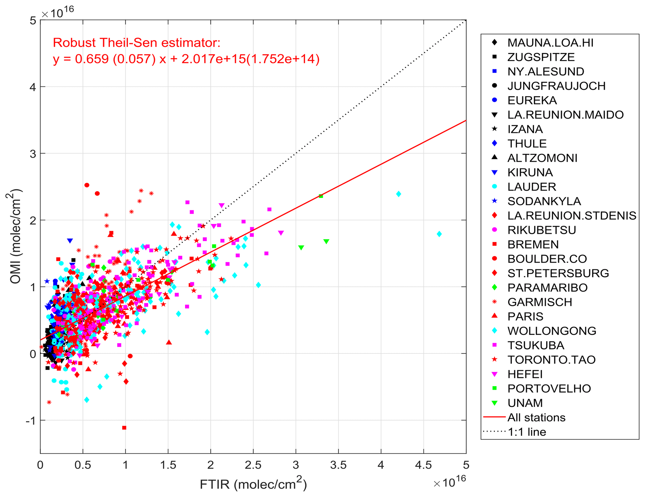
Figure 2 Scatter plot of co-located OMI and FTIR HCHO monthly columns over 2005–2017. The red line represents the Theil-Sen regression. Its slope and intercept (with their 1σ errors between brackets) are given in red.

4.2 OMI HCHO bias determined using aircraft data

Here the OMI data are being evaluated against aircraft in situ measurements, using the regional MAGRITTE model as transfer standard. Figure 3a–c display the distribution of observed HCHO mixing ratios from the three aircraft campaigns. The highest concentrations (>3 ppbv) are seen in the southeast during summertime, whereas lower but still significant levels (1–3 ppbv) are observed over the central USA (Colorado, Nebraska) during summer and over California in winter. The model with a priori emissions reproduces very well the high summer values over the southeast, with very little bias found against SEAC⁴RS data (Fig. 3d–f). Over California and central USA, substantial model underestimations are found, reaching typically a factor of 2. Similar results were obtained by Chen et al. (2019) with the GEOS-Chem model, indicating a good model agreement in regions dominated by biogenic VOC emissions according to MEGAN (i.e., the southeastern USA) and large underestimations over California and the central USA, as shown by extensive comparisons with aircraft campaigns. Not only HCHO but many VOCs are similarly underestimated in those areas (Chen et al., 2019), suggesting the presence of missing VOC sources in emission inventories. Urban VOC emissions are likely strongly underestimated (Karl et al., 2018), likely partly due to the use of volatile chemical products (VCPs) (McDonald et al., 2018) and the underestimation of urban biogenic VOC emissions (Gu et al., 2021). Over Colorado, Nebraska and Texas (among others), fossil fuel exploitation is a large source of alkanes and other VOCs (Pétron et al., 2014; Franco et al., 2016; Tzompa-Sosa et al., 2019), likely responsible for a large part of the model discrepancy.

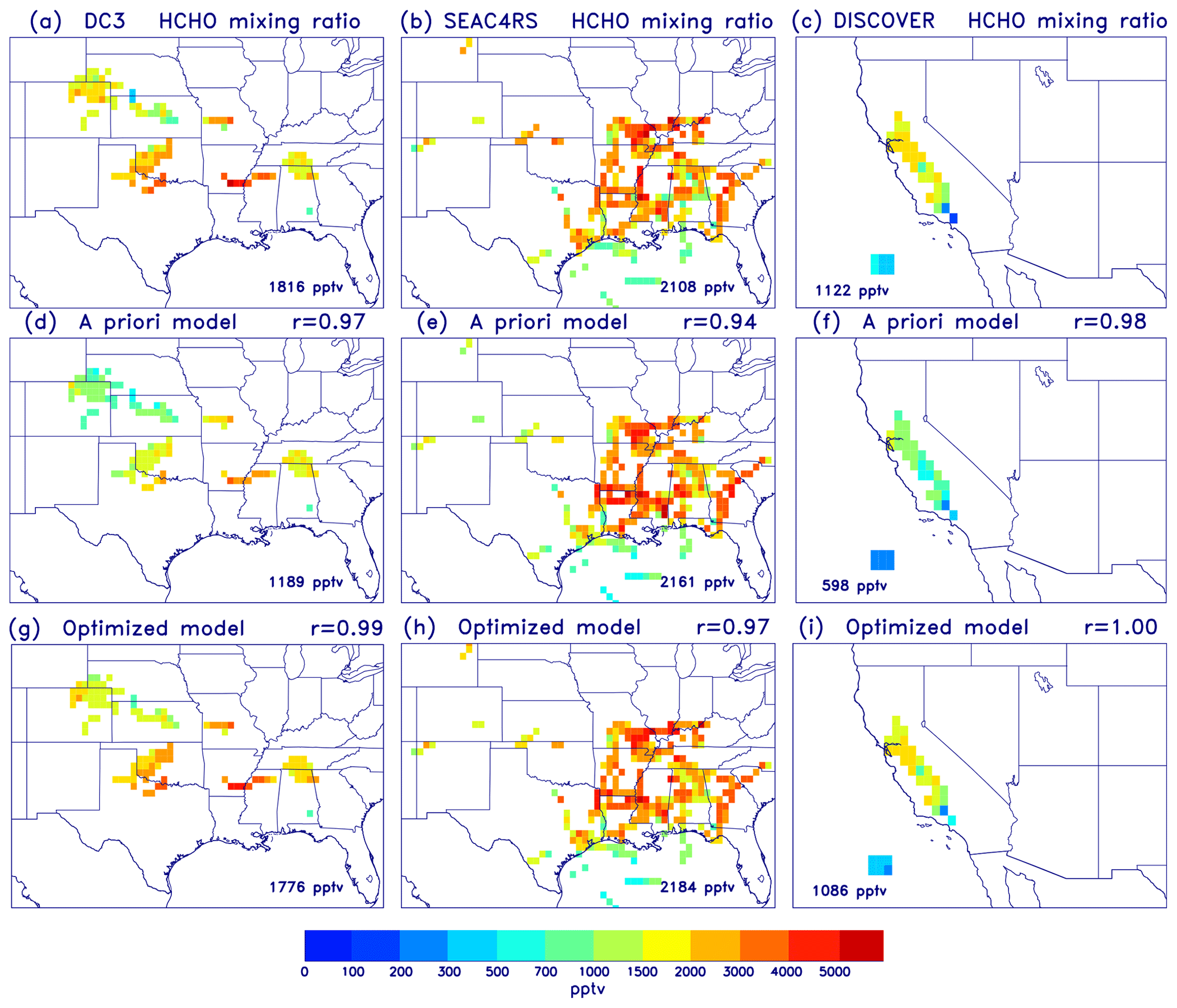
Figure 3 Measured HCHO mixing ratio (pptv) below 4 km altitude from the campaigns (a) DC3, (b) SEAC⁴RS and (c) DISCOVER-AQ California, as well as corresponding model distributions using a priori emissions (d, e, f) and with optimized emissions (g, h, i). Urban and biomass burning plumes were filtered out as described in the text. The data are gridded to the model resolution. The averaged measured or modelled mixing ratio is given for each campaign.

In contrast with the prior simulation, the optimized model using adjusted VOC emissions reproduces very well the observed distributions (Fig. 3g–i), with spatial correlation coefficients of 0.97 or more for each campaign and average biases of at most 3 %. This agreement is achieved through a substantial increase of anthropogenic emissions throughout the USA, whereas biogenic emissions are decreased over much of southeastern USA, and biomass burning emissions undergo a moderate increase (see Table S2 and Fig. S1 in the Supplement). Since the emission parameters are severely underconstrained by the inversion due to the poor coverage of the observations over the model domain, the solution found by the inversion has limited reliability and is strongly dependent on the a priori emission distribution and inversion setup, in particular the covariance matrix of the emission parameters. Despite this caveat, the optimization reproduces very well both the HCHO horizontal distribution (Fig. 3g–i) and the vertical profile shape of HCHO mixing ratios for all campaign datasets, as seen in Fig. 4. While panels (a)–(d) in Fig. 4 display the campaign-averaged profiles for the datasets used in the emission inversion, Fig. 4e shows the profiles for the SENEX campaign which took place in 2013 but was not used as constraint in the inversion. Although the observed profile shape is correctly simulated by the model, the overall agreement is significantly lower for this campaign (−22 % bias) than for the campaign datasets used in the inversion. Given the significant overlap of the SENEX and SEAC⁴RS spatial coverages (see Fig. 1), the underestimation of SENEX HCHO by the model suggests a shift of the summertime biogenic VOC emission peak towards spring, since SENEX and SEAC⁴RS were conducted (primarily) in June and August, respectively. This finding, which is in agreement with the previous determination of isoprene emissions based on satellite (GOME) data by Palmer et al. (2006), will be further examined using OMI and the global model in Sect. 5.

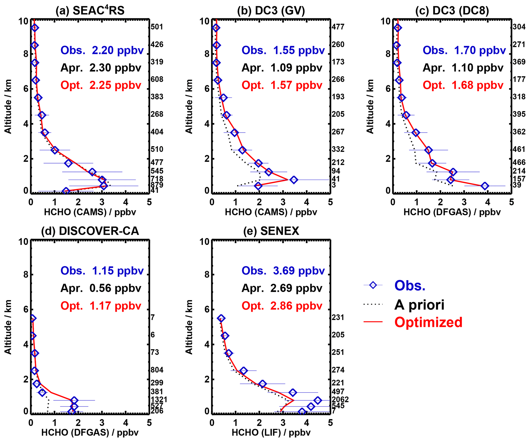
Figure 4 Measured and modelled profiles of HCHO mixing ratios over land (in ppbv) for (a) SEAC⁴RS, (b) DC3 (GV), (c) DC3 (DC-8), (d) DISCOVER-AQ California and (e) SENEX. Urban and biomass burning plumes were filtered out as described in the text. The averaged measured and modelled (a priori and optimized) mixing ratios below 4 km altitude are given for each dataset. The number of observations are given to the right of each plot. The boundaries of the altitude bins are 0, 0.3, 0.6, 1, 1.5, 2, 3, 4, 5, 6, 7, 8, 9 and 10 km. The error bars represent the standard deviation of the measurements.

For the campaigns used in the inversion, a regression of the observed and simulated concentrations yields a slope of almost 1 and a correlation coefficient of 0.93 (Fig. 5a). In contrast with this, Fig. 5b shows that the OMI HCHO columns are significantly biased with respect to co-located columns calculated using the optimized model distributions (Sect. 3.3). High OMI HCHO columns ($>\sim \mathrm{12}\times {\mathrm{10}}^{\mathrm{15}}{\mathrm{molec}.\mathrm{cm}}^{-\mathrm{2}}$) are underestimated by up to ca. 20 % for columns $\sim \mathrm{20}\times {\mathrm{10}}^{\mathrm{15}}{\mathrm{molec}.\mathrm{cm}}^{-\mathrm{2}}$, whereas low columns ($<\sim \mathrm{8}\times {\mathrm{10}}^{\mathrm{15}}{\mathrm{molec}.\mathrm{cm}}^{-\mathrm{2}}$) are generally overestimated. This underestimation of high columns is relatively similar with the slight underestimation (12 %) of OMI HCHO columns from the BIRA V14 product (De Smedt et al., 2015) against SEAC⁴RS HCHO data determined by Zhu et al. (2016). It should be stressed, however, that Zhu et al. (2016) filtered out very negative HCHO columns ($<-\mathrm{5}\times {\mathrm{10}}^{\mathrm{15}}{\mathrm{molec}.\mathrm{cm}}^{-\mathrm{2}}$) from the V14 product, which contributed to increase the campaign-averaged values and reduce the OMI underestimation. Without this filter, the BIRA V14 data are significantly lower than the QA4ECV columns (see Fig. S2). The underestimation of high columns is also qualitatively consistent with the mean OMI bias of −17 % derived by Boeke et al. (2011) for OMI columns $>\mathrm{5}\times {\mathrm{10}}^{\mathrm{15}}{\mathrm{molec}.\mathrm{cm}}^{-\mathrm{2}}$, based on comparisons with several aircraft campaigns conducted in 2008.

A linear regression (Theil-Sen) of OMI and aircraft constrained model columns (Fig. 5b) yields

$$\begin{array}{}\text{(3)}& {\mathrm{\Omega }}_{\mathrm{OMI}}=\mathrm{0.651}{\mathrm{\Omega }}_{\mathrm{airc}}+\mathrm{2.95}\times {\mathrm{10}}^{\mathrm{15}},\end{array}$$

where Ω_OMI and Ω_airc are the HCHO columns (molec. cm⁻²) from OMI and from the aircraft-constrained model simulation, respectively. The regression parameters bear some uncertainty due to aircraft measurement uncertainties. As discussed in Sect. 2.3, the intercomparison of DFGAS and CAMS observations suggests a potential DFGAS overestimation by up to 11 % and a potential bias of our adjusted CAMS concentrations of up to ±6.5 %. Assuming that the optimized model columns are proportional to the observed concentrations, the impact of those potential biases can be estimated through sensitivity regressions. The resulting slope is found to range between 0.6 and 0.7, while the intercept lies in the range (2.6–3.3) $\times {\mathrm{10}}^{\mathrm{15}}{\mathrm{molec}.\mathrm{cm}}^{-\mathrm{2}}$.

The regression given by Eq. (3) is shown as a black line in Fig. 5b and compared with the result of the regression based on FTIR data (see Sect. 4.1), shown as a dashed red line. The slopes of the two regressions are almost identical, but the FTIR-based fit has a smaller intercept and suggests a larger negative bias of high OMI columns than the aircraft-based evaluation. For example, for an OMI column of $\mathrm{18}\times {\mathrm{10}}^{\mathrm{15}}{\mathrm{molec}.\mathrm{cm}}^{-\mathrm{2}}$, the FTIR and aircraft datasets suggest underestimations by factors of 1.35 and 1.29, respectively. There might be several reasons for this, e.g., systematic uncertainties in the measurements and representativeness issues. More importantly, identical results are not expected given the different locations sampled by the two techniques. The OMI bias depends on the magnitude of the column but likely also on other parameters. In absence of additional information, we adopt a bias-correction of OMI data based on both aircraft and FTIR data, shown as the orange line in Fig. 5b. It is obtained by averaging the slopes and intercepts of the regressions of Fig. 2 and Eq. (3). The bias-corrected columns (Ω_OMI,BC) are calculated with

$$\begin{array}{}\text{(4)}& {\mathrm{\Omega }}_{\mathrm{OMI},\mathrm{BC}}=\left({\mathrm{\Omega }}_{\mathrm{OMI}}-\mathrm{2.5}\times {\mathrm{10}}^{\mathrm{15}}\right)/\mathrm{0.655}.\end{array}$$

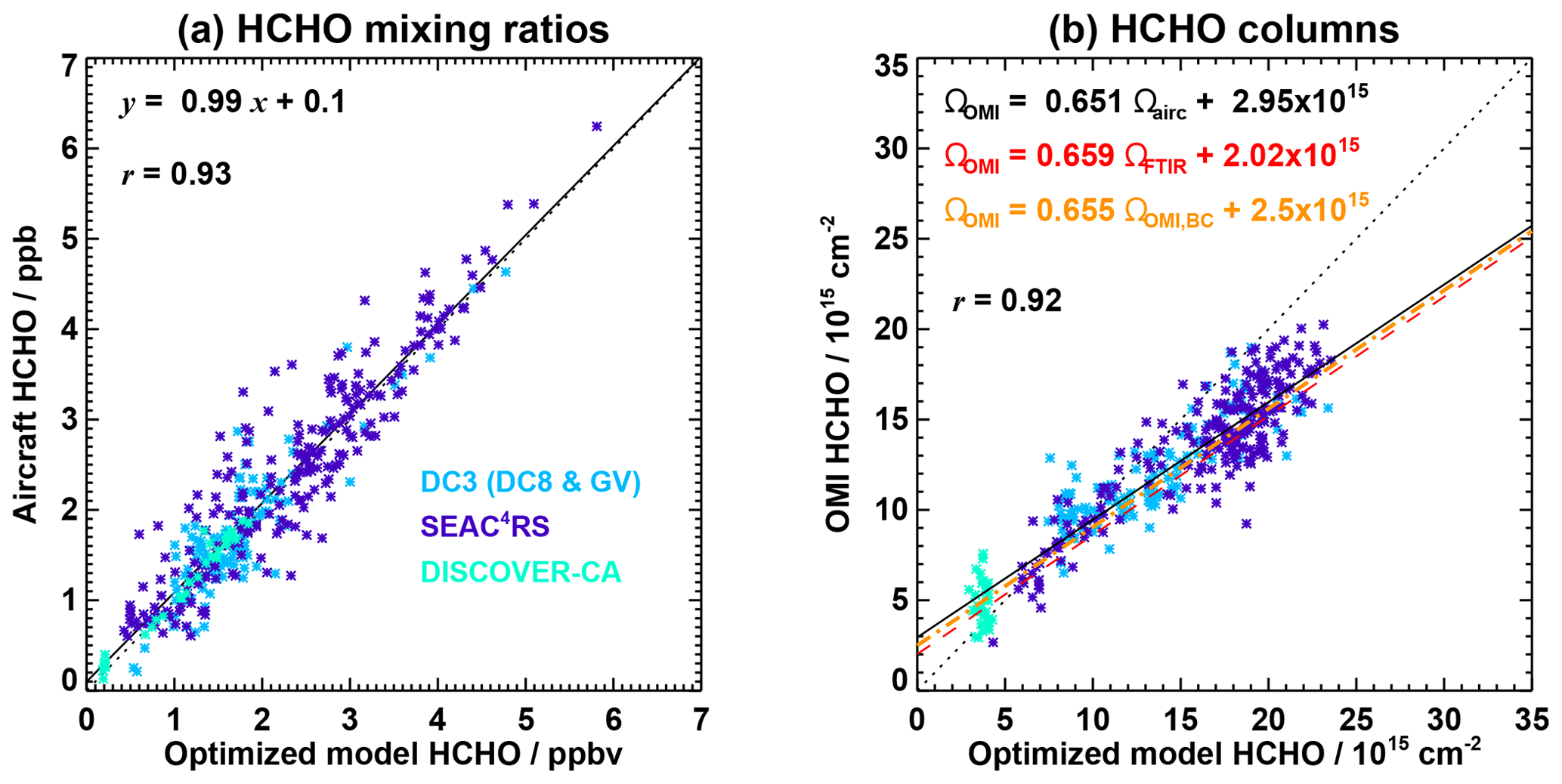
Figure 5 Scatter plots of (a) modelled and observed HCHO mixing ratios (daytime, below 4 km altitude) from three aircraft campaigns (DC3, SEAC⁴RS and DISCOVER-AQ California) and (b) modelled and OMI total HCHO columns at the same model pixels as in panel (a). The modelled values are constrained by the aircraft measurements through an emission optimization as described in the main text. The correlation coefficient and regression parameters using the Theil-Sen estimator are given in each panel (black font) and shown as a solid black line. The slope and intercept of the regression of OMI columns vs. FTIR data (see Sect. 4.1) are given in panel (b) (red font) and shown as a dashed red line. The adopted bias correction (relationship between OMI columns Ω_OMI and bias-corrected columns Ω_OMI,BC) are also given (orange) and shown as the dash-dotted orange line.

The resulting correction enhances columns above $\sim \mathrm{7}\times {\mathrm{10}}^{\mathrm{15}}{\mathrm{molec}.\mathrm{cm}}^{-\mathrm{2}}$ and decreases columns below that value. The contrasts between high- and low-emission regions will therefore be strengthened by the bias correction.

Note that the standard QA4ECV cloud-corrected v1.2 product shows very similar biases with respect to aircraft data as the cloud-uncorrected product evaluated above. The evaluation of the standard product (CF <0.4, with cloud correction) yields a slope of 0.68 and an intercept of $\mathrm{2.6}\times {\mathrm{10}}^{\mathrm{15}}{\mathrm{molec}.\mathrm{cm}}^{-\mathrm{2}}$ (see Fig. S2).

5 Inferring emissions from bias-corrected OMI HCHO columns

5.1 Impact of bias correction on top-down VOC emissions

The global emission inversions are labeled as indicated in Table 2. OPT1 is conducted without any bias correction to the OMI HCHO columns, whereas OPT2 uses bias-corrected columns obtained from Eq. (4). OPT3 is a sensitivity test aimed at determining the influence of prior errors on the emission parameters. The errors on all emission parameters are taken to be a factor of ∼4 (e^1.4) in this case (instead of a factor of $e^{\mathrm{1.1}}=\sim \mathrm{3}$ in OPT1 and OPT2; see Sect. 3.3).

Table 2 Global emission optimizations conducted in this work.

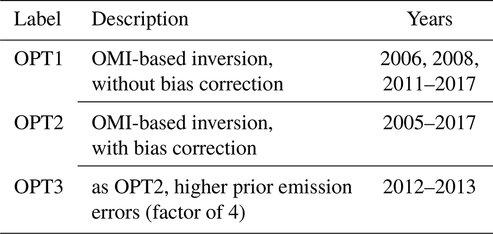
Figure 6 shows seasonally averaged HCHO columns from OMI (bias-corrected), the a priori simulation and the OPT2 simulation. Although the a priori simulation reproduces many features of the observations, there are noticeable differences, such as overestimated columns over Australia and Paraguay in December–January–February (DJF) and underestimated columns over southern Africa, Europe, east and south Asia in both DJF and June–July–August (JJA). The overestimation over Australia might be partly due to the high emission rates used in MEGANv2.1, based on measurements for young eucalypt trees which may emit more isoprene than adult trees (Emmerson et al., 2016).

As expected, the optimization realizes a much better agreement with the data, especially in areas with strong signal, such as tropical regions during DJF and JJA and the eastern USA, China and India during summer. Model underestimations remain significant over regions with relatively low columns, such as the western USA and Europe, where the relative errors in the data are larger, particularly in winter; the retrieval error is typically 40 %–50 % over high-emission areas (e.g., tropical forests) and 50 %–100 % over low-emission regions (e.g., western Europe).

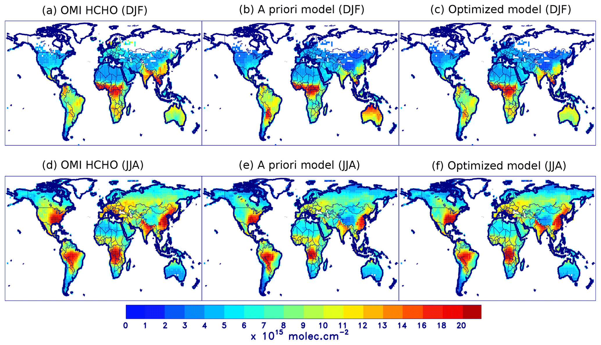
Figure 6 2005–2017 average of HCHO columns (${\mathrm{10}}^{\mathrm{15}}{\mathrm{molec}.\mathrm{cm}}^{-\mathrm{2}}$) in December–January–February (DJF) from (a) OMI (bias-corrected as described in the text), (b) the a priori model and (c) the model with optimized emissions. Panels (d)–(e) are the same as panels (a)–(c) but for June–July–August (JJA).

The improved simulation of HCHO columns from Fig. 6 is realized through significant changes in the amount and distribution of VOC emissions. Figure 7 displays the distribution of the emission ratios (optimized flux/a priori flux) per emission category for both optimizations, OPT1 and OPT2 (2011–2017 average). The mean annual emission totals in large regions are given in Table 3 for OPT2 (for 2005–2017) and in Table S3 for both OPT1 and OPT2 over 2011–2017.

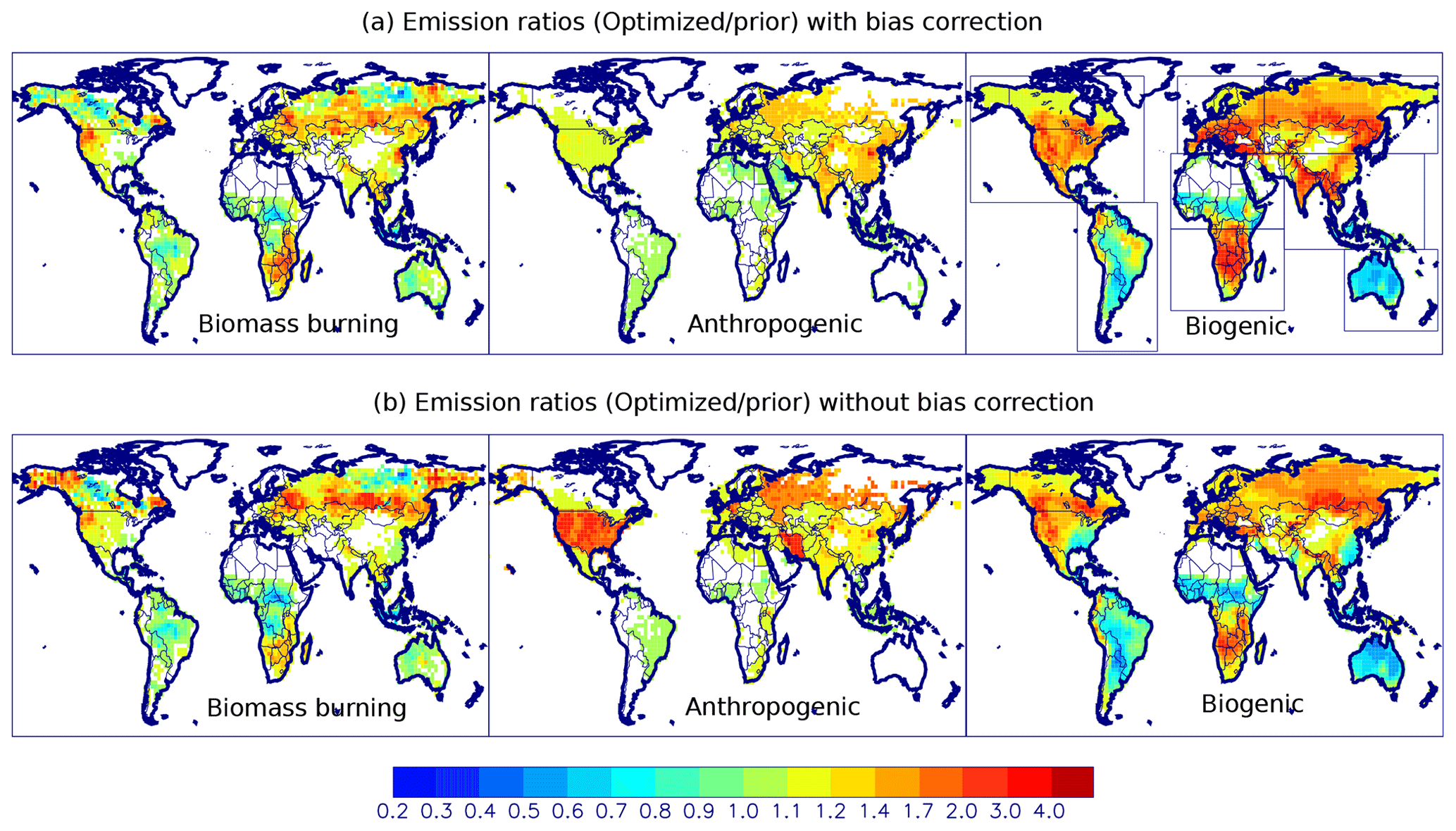
Figure 7 Ratios of top-down emissions to a priori emissions (2011–2017 average) for biomass burning VOCs (left panel), anthropogenic VOCs (middle) and biogenic VOCs (right) for optimizations (a) OPT2, constrained by bias-corrected columns, and (b) OPT1, constrained by uncorrected columns. Pixels with very small emission changes (<1 %) are left blank. The regions used for calculation of total emissions given in Table 3 are shown as boxes on the top right panel.

Table 3 Mean a priori and OMI-based (OPT2) emission estimates (Tg yr⁻¹) per source category for different world regions and globally. Regions are defined in Fig. 7. The means are taken either over 2005–2017 (OPT2 simulation period) or 2005–2013 (for comparison with Bauwens et al., 2016). B16: Bauwens et al. (2016). NH: Northern Hemisphere; SH: Southern Hemisphere.

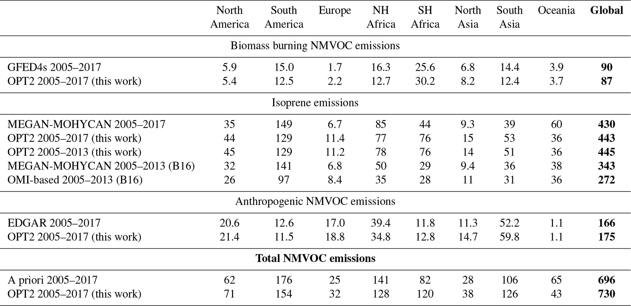
The bias correction of OMI columns has a large impact on the inferred top-down emissions (Fig. S4), especially for the biogenic emission category, which is the dominant contribution to HCHO columns over continental regions (Stavrakou et al., 2009). Without bias correction, global isoprene emissions are decreased from 430 Tg yr⁻¹ in the a priori from MEGAN (2011–2017 period, Table S3) to 362 Tg yr⁻¹ in optimization OPT1 (i.e., a 16 % decrease), whereas OPT2 increases those emissions by about 5 % to 451 Tg yr⁻¹. The impact is strongest over south Asia (+43 % difference between OPT1 and OPT2). It is also striking over many other regions, such as the eastern USA and southern China (Fig. 7), where biogenic emissions are decreased by up to over 30 % in OPT1 but are increased in OPT2. In other regions such as the high latitudes and Australia, the difference is lower or even negative. This result is expected, given the lower columns in these regions (typically below ${\mathrm{10}}^{\mathrm{16}}{\mathrm{molec}.\mathrm{cm}}^{-\mathrm{2}}$), implying that the bias correction leads to only slight HCHO increases or even to HCHO decreases.

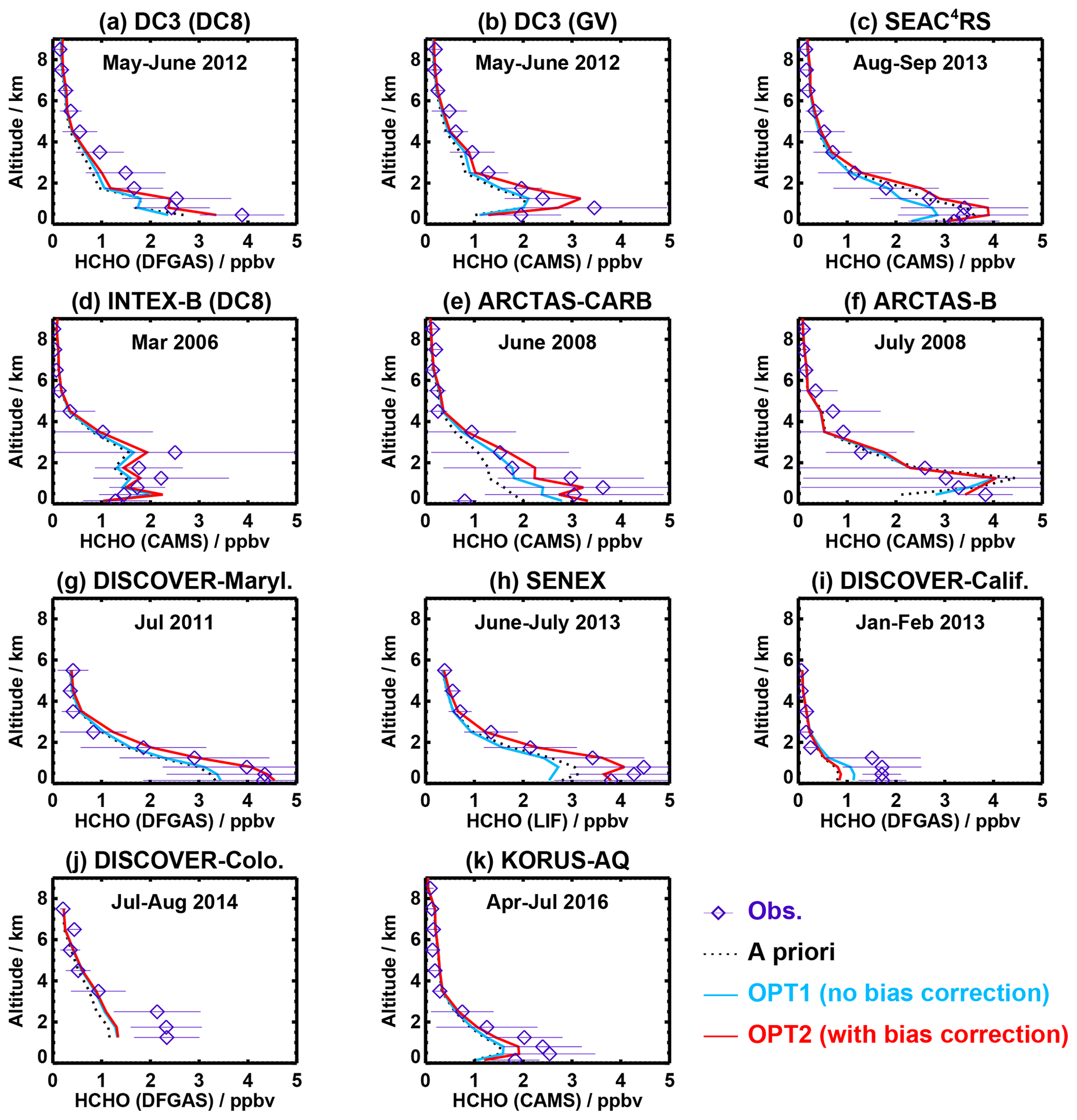
Figure 8 Measured and modelled profiles of HCHO mixing ratios over land (in ppbv) for (a) DC3 (DC-8), (b) DC3 (GV), (c) SEAC⁴RS, (d) MILAGRO, (e) ARCTAS-CARB, (f) ARCTAS-B, (g) DISCOVER-AQ Maryland, (h) SENEX, (i) DISCOVER-AQ California, (j) DISCOVER-AQ Colorado and (k) KORUS-AQ. Optimization constrained by either uncorrected OMI columns (OPT1, in blue) or bias-corrected columns (OPT2, in red). The error bars represent the standard deviation of the measurements. Comparison statistics are provided in Table S4.

The top-down global isoprene emissions from OPT2 (445 Tg yr⁻¹ for 2005–2013) are a factor of 1.64 higher than the top-down emissions derived by inverse modelling of OMI data by Bauwens et al. (2016) (272 Tg yr⁻¹). The optimized emissions of the OPT3 run (with higher a priori emission errors) are even slightly higher (by 3 %) than in OPT2. Note that our a priori (MEGAN) emissions are also higher than in Bauwens et al. (2016), especially over Australia and Africa, due to the soil moisture stress impact that was accounted for by Bauwens et al. (2016) but not in our study (Sect. 3.2). The bias correction of OMI data applied in this work explains only a part (factor 1.25) of the large discrepancy between the top-down estimates. The main reason for the remainder is the different OMI retrieval (BIRA-V14) (De Smedt et al., 2015) used as constraint in Bauwens et al. (2016). The BIRA-V14 HCHO columns are indeed significantly lower than the QA4ECV data used here, as already noted by Wells et al. (2020). As shown in Fig. S3, QA4ECV columns are typically higher than the V14 product by 10 %–50 % over continents, and by up to 80 % in parts of southern Africa. This explains why the OPT1 isoprene emissions over Southern Hemisphere Africa, 60 Tg yr⁻¹, are about a factor of 2 higher than the top-down estimate from Bauwens et al. (2016), whereas the two top-down estimates are in much better agreement over South America and Australia, where the QA4ECV and V14 HCHO columns are more similar (Fig. S3).

The effect of the bias correction on the optimized emissions is obtained by comparing the OPT1 and OPT2 top-down emissions. The bias correction increases the top-down biogenic emissions (by a factor of 1.25 at global scale) and biomass burning emissions (factor of 1.13) and decreases the anthropogenic emissions at middle and high latitudes, except over China (Table S3 and Fig. 7). This is primarily due to the generally low HCHO columns during winter in those regions, typically below $\mathrm{6.5}\times {\mathrm{10}}^{\mathrm{15}}{\mathrm{molec}.\mathrm{cm}}^{-\mathrm{2}}$, for which the bias correction decreases the columns (Eq. 4). The exacerbated seasonal variation of the HCHO columns due to the bias correction favors the biogenic emissions to the detriment of anthropogenic sources at these latitudes. This result is highly dependent on the HCHO column uncertainties, however. The scatter plots of Figs. 2 and 5 show a large dispersion for low columns, indicating high uncertainty in the bias correction. For this reason, the optimization results should be considered with caution in low-column areas.

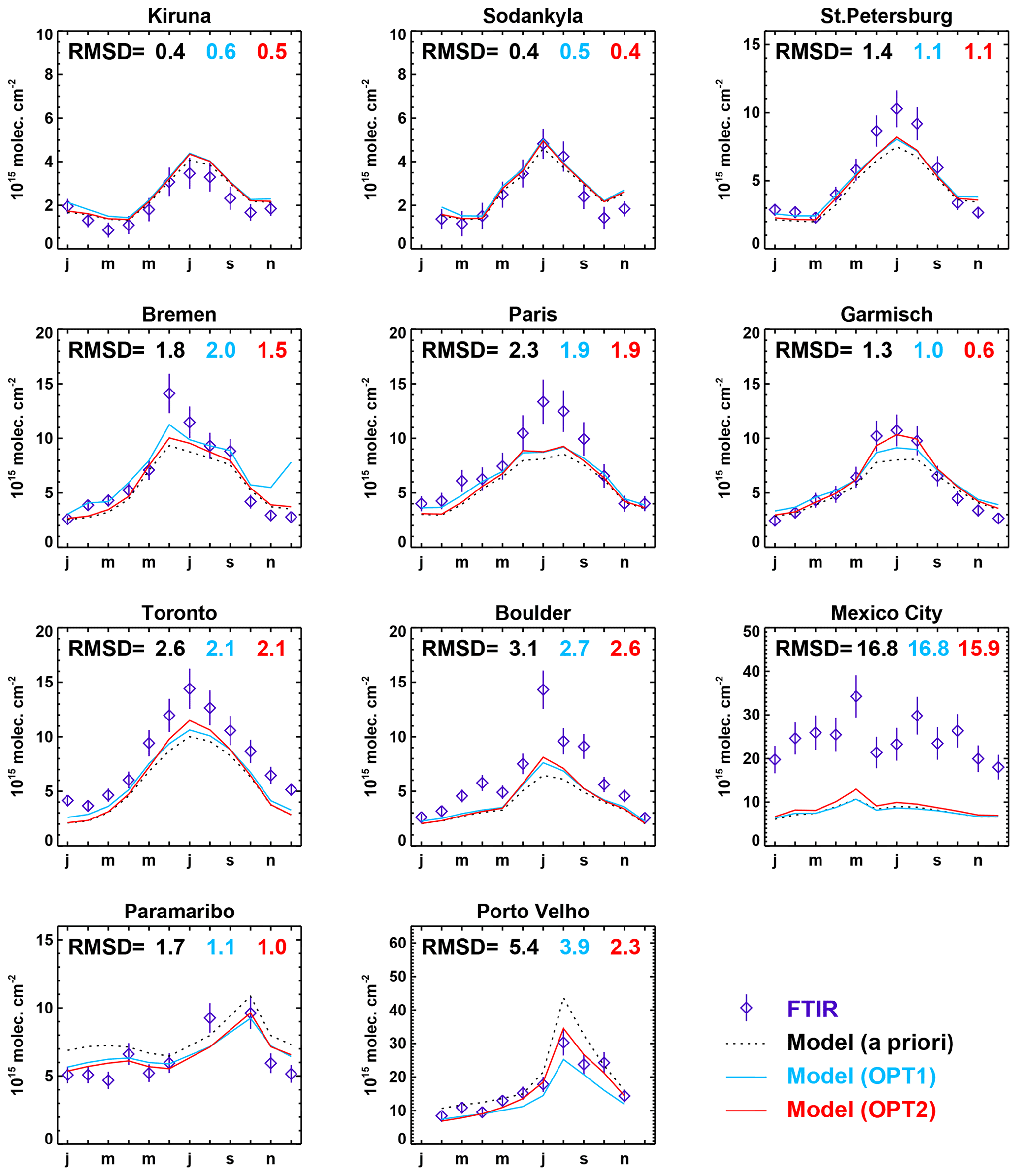
Figure 9 Average seasonal cycle of HCHO columns at FTIR stations (2011–2017). Symbols with error bars represent the mean FTIR columns and related systematic uncertainties. Black dotted curve: model with a priori emissions; blue curve: OPT1 simulation constrained by uncorrected OMI columns; red curve: OPT2 simulation constrained by bias-corrected OMI columns. The root mean square deviation (RMSD) of the three model runs is given for each station.

5.2 Evaluation of optimized HCHO against aircraft and FTIR data

The optimizations OPT1 and OPT2 were conducted over years (Table 2) for which aircraft campaign data are available, over the USA, Canada, Mexico and South Korea (Fig. 1 and Table 1). Figure 8 displays the mean observed and modelled vertical HCHO profiles for all campaigns. For most campaigns, the model agreement is improved when the bias correction is applied to the satellite columns. On average for all campaigns, the large negative bias found for both the a priori simulation (−27 %) and the OPT1 run (−28 %) is strongly reduced in the OPT2 run (−9 %) (Table S4). The root mean square deviation (RMSD) is also decreased, from 0.85 and 0.86 ppbv in the a priori and OPT1 run to 0.55 ppbv in the OPT2 run. In particular, OPT2 presents very little biases over high-column areas (e.g., DC3, SEAC⁴RS, SENEX). The observed horizontal distribution of the vertically averaged HCHO mixing ratios is also very well matched by the model over high-emission regions in the eastern USA, with Pearson's correlation coefficients ranging between 0.96 and 0.98 after optimization for those campaigns (Fig. S5). The results of the OPT3 optimization are similar to or even slightly better (for SEAC⁴RS and for DC3 DC-8) than those of OPT2 (Table S4).

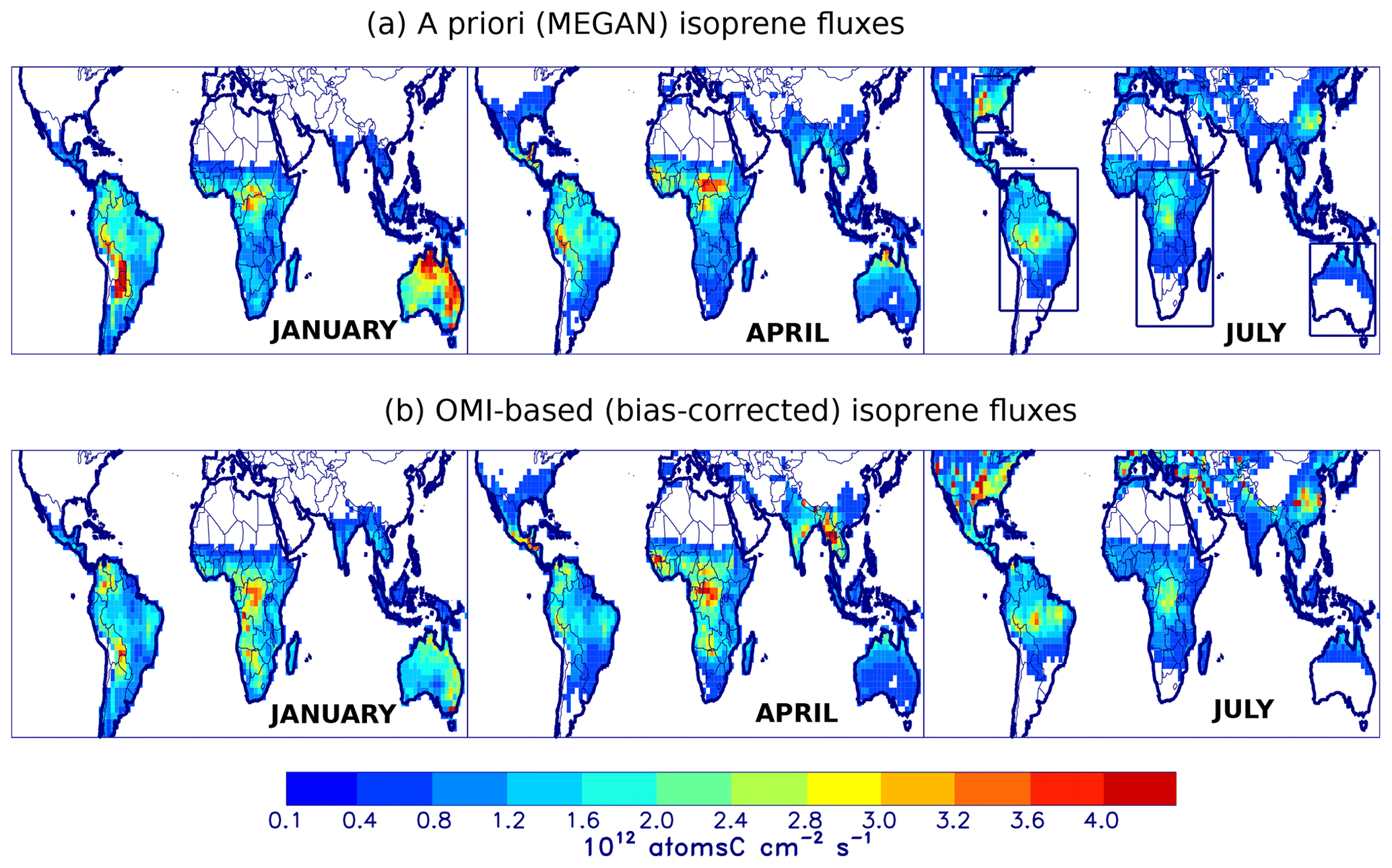
Figure 10 (a) A priori (MEGAN) isoprene monthly fluxes (10¹² atoms C cm⁻² s⁻¹) in year 2013. (b) Optimized isoprene fluxes based on (bias-corrected) OMI HCHO columns, also for 2013. The boxes shown in the July a priori flux subplot show the regions for which emission totals are displayed in Fig. 11.

In contrast with this good performance, OPT2 presents large underestimations over low-emission areas over the western USA, namely, the DISCOVER campaigns in Colorado (−43 % bias) and California (−53 %). Low OMI columns were measured during the latter campaign (Jan.–Feb. 2013), in the range (3–6) $\times {\mathrm{10}}^{\mathrm{15}}{\mathrm{molec}.\mathrm{cm}}^{-\mathrm{2}}$, such that the bias correction further decreased the columns. The OMI columns were higher during DISCOVER-Colorado ($\sim \mathrm{7}\times {\mathrm{10}}^{\mathrm{15}}{\mathrm{molec}.\mathrm{cm}}^{-\mathrm{2}}$ near Boulder, Colorado, in July–August 2014), but the modelled columns remained much underestimated (by 0 %–40 %) after emission optimization, due to the large OMI column uncertainties.

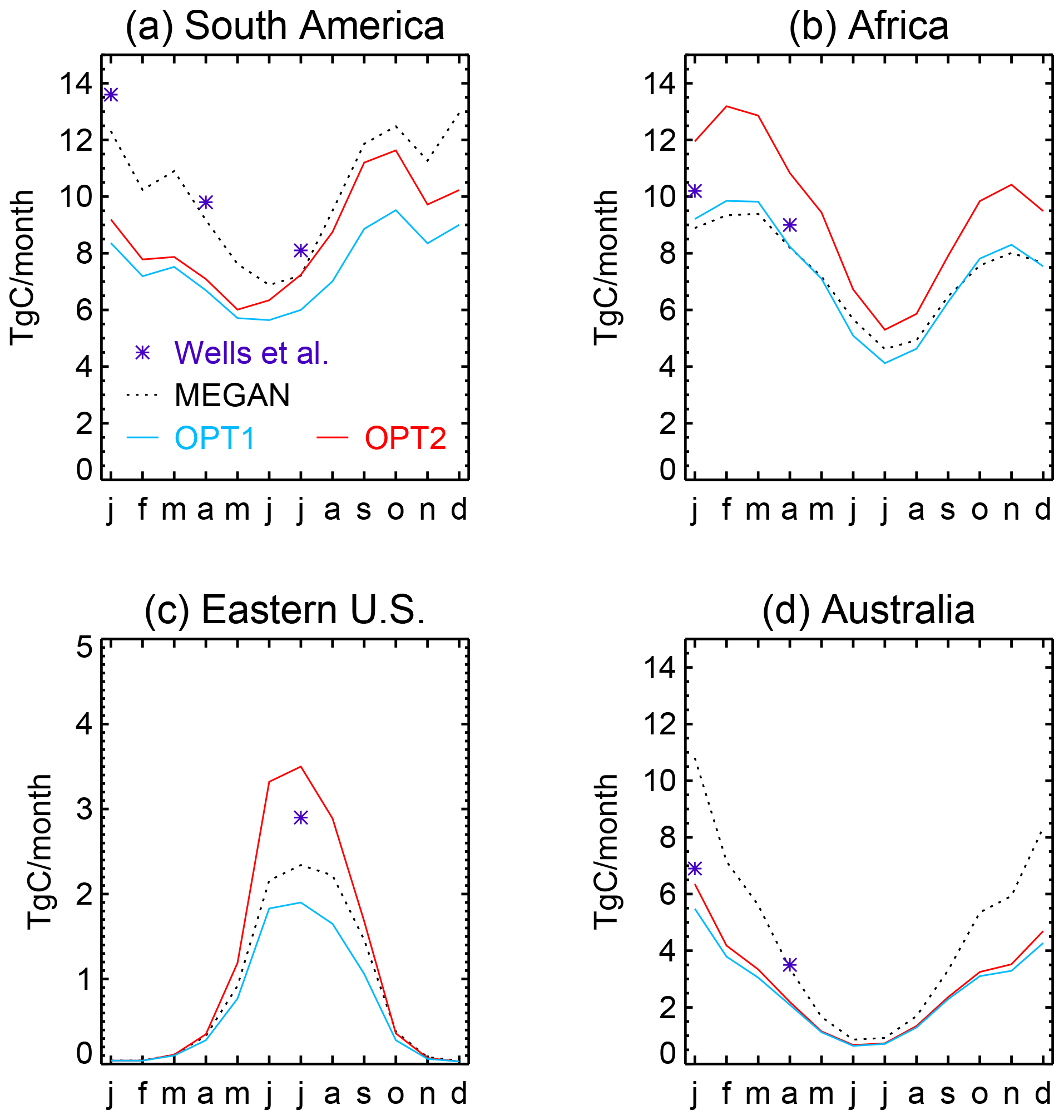
Figure 11 Seasonal variation of isoprene monthly fluxes (2013) in (a) South America (82.5–32.5^∘ W, 32^∘ S–14^∘ N), (b) Africa (5–52.5^∘ E, 36^∘ S–14^∘ N), (c) southeastern USA (75–100^∘ W, 26–42^∘ N) and (d) Australia (115–155^∘ E, 10–40^∘ S). Results shown for the a priori inventory (MEGAN, dotted line), the OMI-based optimizations (OPT1 in blue, OPT2 in red) and the CrIS-based optimization results from Wells et al. (2020) (asterisks).

Figure 9 displays the mean observed and modelled seasonal evolution of HCHO columns at 11 FTIR stations located in source regions. The other stations (primarily high-altitude, high-latitude or maritime stations) show little sensitivity to VOC emission changes. The complete time series (2005–2017) of monthly observed and modelled (OPT2) HCHO columns are shown in the Supplement (Figs. S6 and S7). The impact of the emission optimizations is relatively small at middle and high latitudes and largest at the two South American stations (Paramaribo and Porto Velho). The OPT2 run performs better than OPT1, with lower RMSD values at all sites and lower biases at 8 out of 11 sites (Table S5). The OPT2 run also performs better than the prior simulation at all sites except Kiruna and Sodankylä in northern Scandinavia, where the moderate biogenic emission increase inferred by the optimization (Fig. 7) enhances the small positive model bias which was already present in the a priori simulation.

At the other European stations and at North American sites, the emission increase of the OPT2 run improves the agreement with the measurements but fails to close the gap completely (except at Garmisch), in particular during summer. This discrepancy is mostly explained by the model underestimation of OMI columns after optimization, as seen in Figs. 6 and S8. The exception is Mexico City, where the model successfully matches the OMI columns (Fig. S8) but underestimates the FTIR columns by about a factor of 3. This poor model performance can be attributed to the coarse model resolution (2^∘ × 2.5^∘) being unable to resolve the megacity emissions. At Boulder, the model underestimation of both OMI and FTIR columns (by up to a factor of 2 in summer) is consistent with the model underestimation against airborne HCHO data from DISCOVER-Colorado, by almost a factor of 2 (Fig. 8).

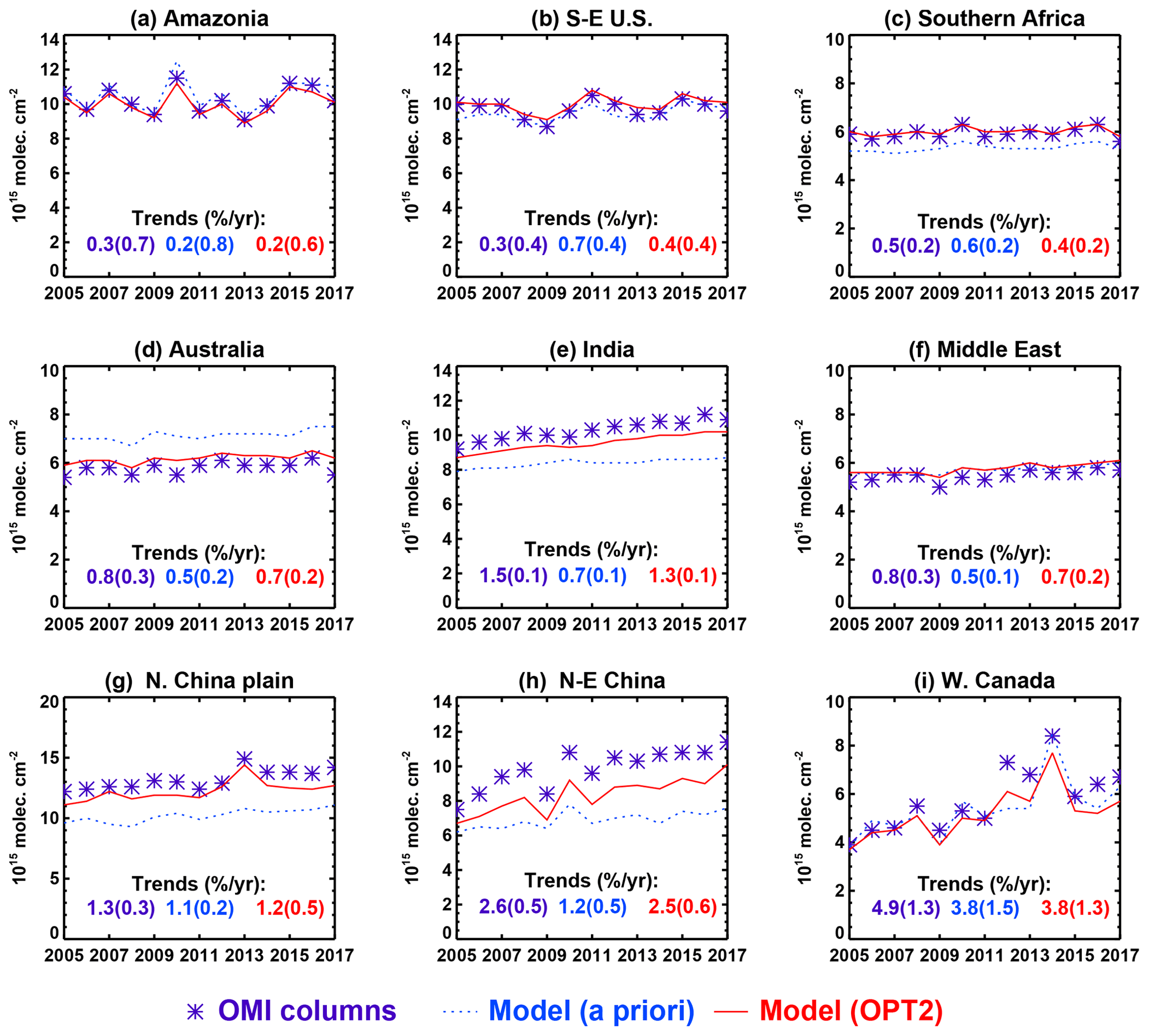
Figure 12 Annually averaged (bias-corrected) HCHO columns (2005–2017) averaged over (a) Amazonia (40–75^∘ W, 20^∘ S–5^∘ N), (b) S-E USA (75–100^∘ W, 26–36^∘ N), (c) southern Africa (20^∘ W–65^∘ E, 0–40^∘ S), (d) Australia (110–155^∘ E, 10–38^∘ S), (e) India (67–92^∘ E, 10–30^∘ N), (f) the Middle East (40–55^∘ E, 26–42^∘ N), (g) North China Plain (112–122^∘ E, 32–40^∘ N), (h) N-E China (122–132^∘ E, 42–50^∘ N) and (i) W Canada (100–120^∘ W, 54–64^∘ N). Linear regression trends (2005–2016) are given, with their 1σ uncertainty between brackets. OMI: violet symbols; a priori model in blue, optimized model (OPT2) in red.

The comparison at the Amazonian sites of Paramaribo (Suriname) and Porto Velho (Rondônia, southwestern Brazil) validates the VOC emission decrease (by ∼20 %) inferred by OPT2 during the dry season (July–November). The stronger emission decrease of the OPT1 run in Rondônia (factor of 2) leads to a significant model underestimation of FTIR HCHO columns at Porto Velho. At both sites, biogenic emissions are also strongly decreased in the first half of the year (up to a factor of 3 at Porto Velho in February 2017). This decrease at Porto Velho is due to very low HCHO columns observed by OMI in the first months of 2017, especially February (Fig. S8).

5.3 Evaluation of top-down isoprene emissions

The major source regions of biogenic isoprene according to the MEGAN model are South America, sub-Saharan Africa, Australia, the eastern USA and south Asia, including southern China (Fig. 10a). The fluxes display a pronounced seasonality reflecting, primarily, their dependence on temperature and radiation (Guenther et al., 2006), with clear maxima during summertime, except near the Equator. In January 2013, the highest fluxes are predicted in a region centered over Paraguay in South America as well as over northern and eastern Australia; in April, near the Peru–Brazil border region and especially over the Central African Republic (CAR) and South Sudan; and in July, in the US states bordering the Mississippi River below 38^∘ N latitude.

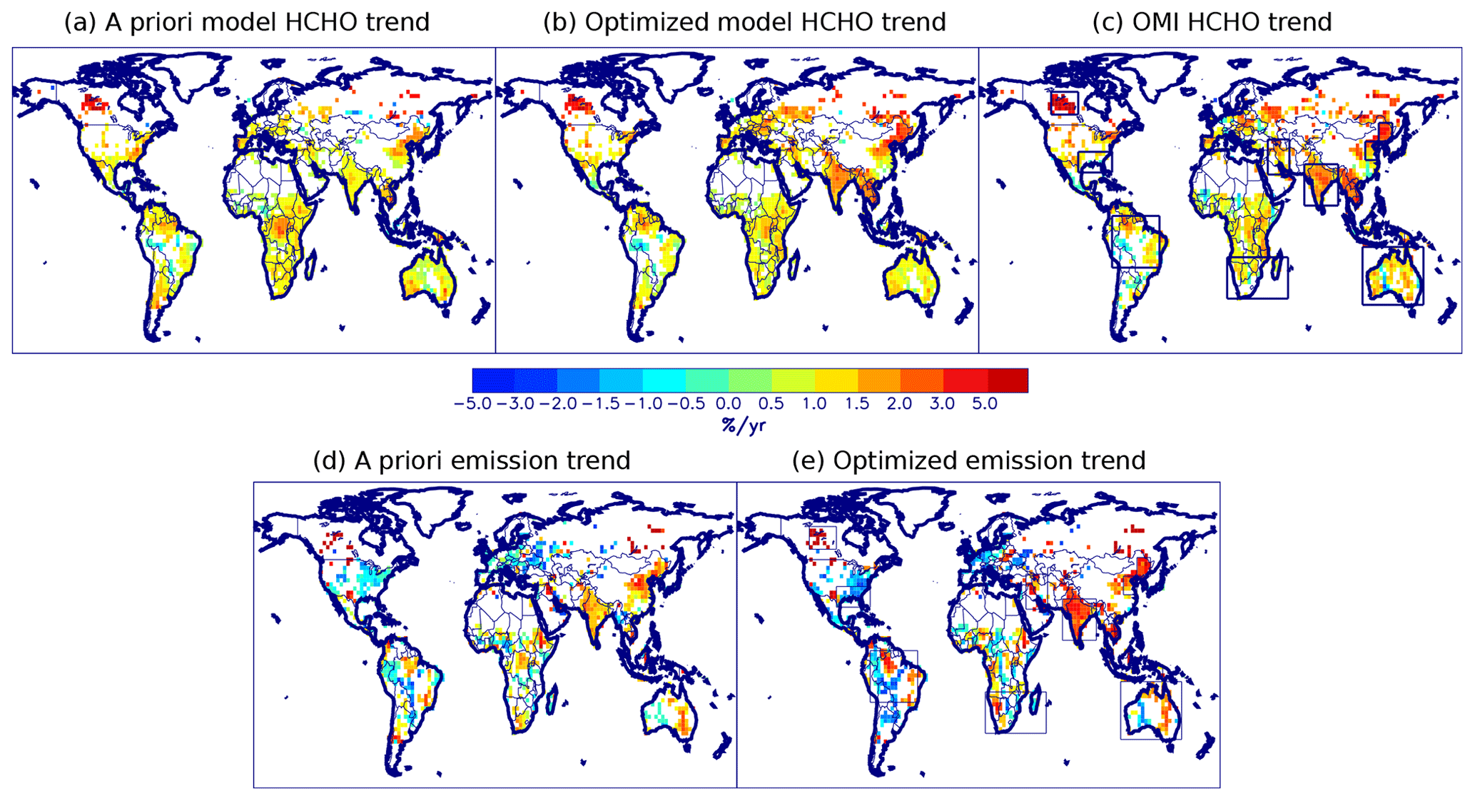
Figure 13 Trends (% yr⁻¹) over 2005–2016 of yearly averaged HCHO columns from (a) the a priori model simulation, (b) the optimized (OPT2) simulation, (c) the bias-corrected OMI retrieval, and trends of total NMVOC emissions from (d) the a priori simulation and (e) the OPT2 simulation. Pixels with low a priori emission (below $\mathrm{5}\times {\mathrm{10}}^{\mathrm{10}}{\mathrm{molec}.\mathrm{cm}}^{-\mathrm{2}}{\mathrm{s}}^{-\mathrm{1}}$) or for which the trend uncertainty exceeds 150 % of the trend are left as blank. The boxes in panels (c) and (e) show the regions used for calculating the temporal evolution of averaged columns (Fig. 12) and total emissions (Fig. 14).

The OMI-based optimization (OPT2) leads to substantial changes in the distribution of isoprene emissions. As seen in Fig. 10, sharp declines are predicted over most hotspots mentioned above, most noticeably those over Paraguay, the CAR, Australia and the Peru–Brazil border. Emission decreases are also found over the Guianas and Indonesia, especially in January. Other regions emerge as important source regions, most prominently the Congo Basin and a vast area in southwestern Africa spanning Angola, Namibia and Botswana. Although the distributions shown in Fig. 10 are for the year 2013, similar features and emission updates are derived for all years (see Sect. 5.4 for a discussion of interannual variability).

Those emission updates are in good qualitative agreement with optimized isoprene emissions based on isoprene column densities from the spaceborne Cross-track Infrared Sounder (CrIS) for the same year (2013) (Wells et al., 2020). Those authors applied an iterative mass balance technique to optimize the emissions of isoprene in the GEOS-Chem model, using as constraints the first global retrieval of isoprene columns from space. Due to the critical role played by hydroxyl radical (OH) levels in this emission inversion and given the strong influence of nitrogen oxides (NO_x) on OH, the NO_x emissions in GEOS-Chem were optimized based on spaceborne NO₂ data before conducting the isoprene inversion. The CrIS-derived monthly-averaged emissions (Figs. 12–15 in the Supplement in Wells et al., 2020) display striking similarities and differences with the OMI-constrained distributions of Fig. 10b. Common features include the decreases over Paraguay, the Guianas, the Peru–Brazil border, and the CAR and South Sudan region, as well as the increases over the Congo and southwestern Africa as well as Colombia and central US states spanning from Texas to Illinois. Despite very different a priori isoprene emissions over Australia (e.g., respectively 10.8 and 4.2 Tg in January in our inventory and in  Wells et al., 2020), the CrIS-based total emissions over the continent are slightly higher than our OMI-based values (Fig. 11). Closer examination shows a good agreement in the eastern part, whereas the CrIS-based emissions appear to be higher in the north and lower in the central part of the country, compared to our estimates (Fig. 10). The OMI-based emissions are significantly lower than both the a priori estimate and the CrIS-based fluxes over South America in January and April, whereas the opposite holds over Africa (Fig. 11). The discrepancy is largest over Brazil, where OMI columns as low as $\mathrm{6}\times {\mathrm{10}}^{\mathrm{15}}{\mathrm{molec}.\mathrm{cm}}^{-\mathrm{2}}$ are frequently observed during the wet season (December–May). Those low values drive a decrease in biogenic emissions, reaching ca. 20 %–30 % over western and northern Brazil. As discussed in Sect. 5.2, the optimized model underestimates FTIR data in February–May at Porto Velho, due to excessively low OMI columns (in February). Although the Porto Velho comparison was for a different year (2017), it suggests that the wet season OMI data might be less reliable, possibly due to high cloudiness in the area. In July, a very good agreement is found between the CrIS-based and OMI-based emissions over South America, in terms of distribution and total. Over Africa, the discrepancy is largest in January over the CAR, in a region with strong fire emissions in several biomass burning inventories including GFED4s (Pan et al., 2020). Both pyrogenic and biogenic VOC emissions are strongly reduced in this region by the OMI-based inversion, as in several previous inverse modelling studies (e.g., Bauwens et al., 2016; Müller et al., 2018), but the interference of strong pyrogenic emissions makes the top-down isoprene estimate particularly uncertain and likely contributes to the differences with CrIS-based results. Interference from biomass burning probably plays a role in other regions as well, especially southern Africa in June–September, the southern part of Amazonia in August–September, southeast Asia in February–April and boreal forests during June–August. In most other regions and periods, the discrimination between pyrogenic and biogenic emissions is less critical, given the general dominance of biogenic VOCs over biomass burning as source of HCHO (Stavrakou et al., 2009, 2018). In addition, the derivation of isoprene emissions from CrIS data also has its limitation, most importantly the role played by the assumed isoprene vertical profile in the retrieval of the total column (Wells et al., 2022) and the strong impact of OH radical concentrations on CrIS-derived emissions (Wells et al., 2020).

Figure 14 (a)–(d) Total isoprene emissions and (e)–(h) total VOC annual emissions (Tg yr⁻¹) from the same large regions as in Fig. 12. A priori emissions are in blue; optimized emissions (OPT2) are in red. Linear regression trends (2005–2016) are given, with their 1σ uncertainty in brackets.

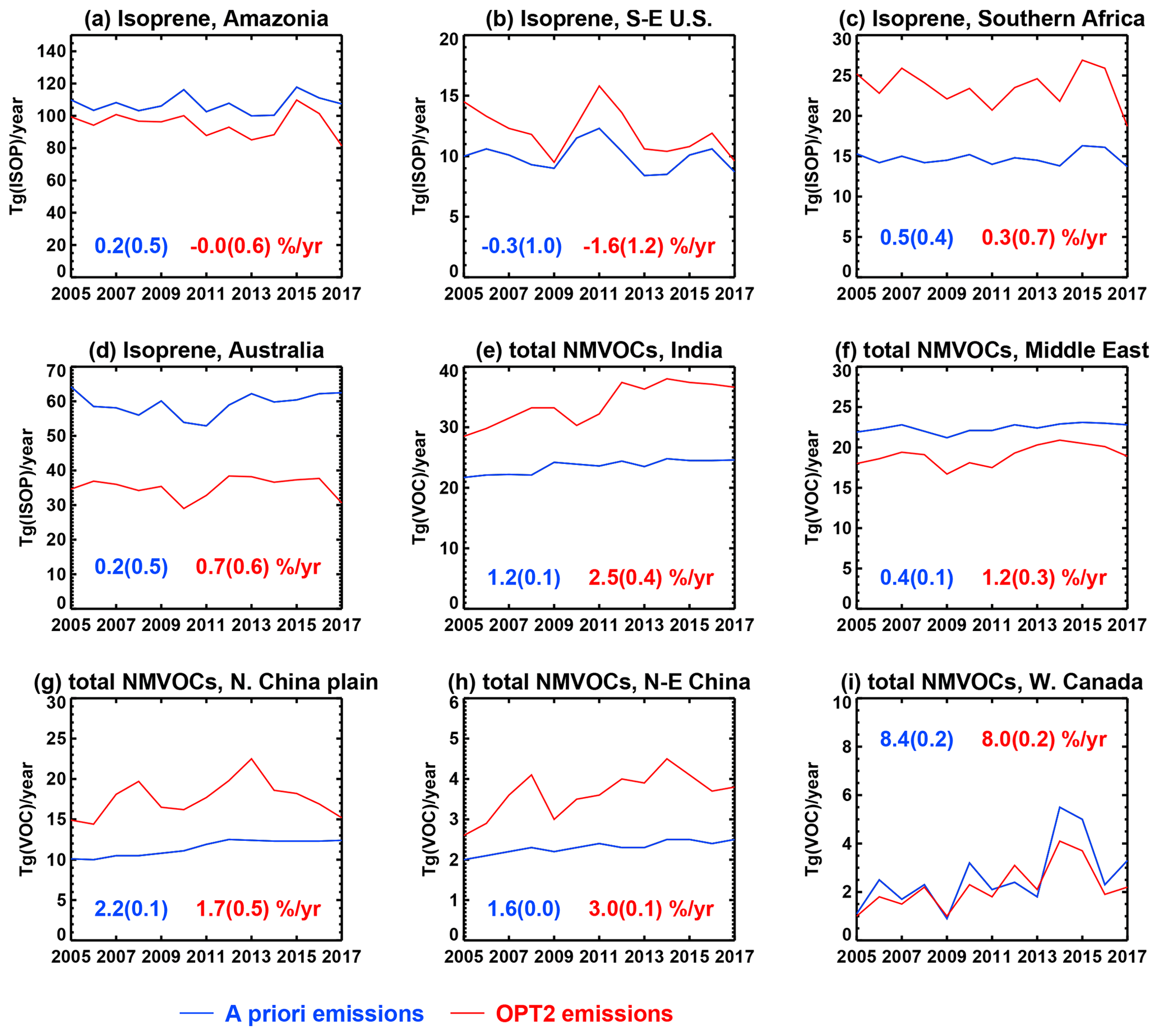
5.4 Trends of HCHO columns and VOC emissions

Figure 12 displays the temporal evolution of annually averaged (bias-corrected) OMI and modelled columns over large regions. The contours of those regions are shown in Fig. 13, which displays the distribution of percentage trends of HCHO columns (panels a–c) and total VOC emissions (d–e) between 2005 and 2016. All trends are obtained using a simple least-squares regression method.

Already without emission optimization, the modelled columns are strongly correlated temporally with the observations over regions where biogenic VOC emissions and biomass burning are the dominant sources of HCHO. Interannual variability over those regions is primarily related to climate variables (temperature and radiation) through their influence on biogenic emissions, biomass burning and background HCHO (Stavrakou et al., 2018), and the good model performance suggests that the inventories used in the model (MEGAN-MOHYCAN and GFED4s) are generally adequate. The year 2017 stands out in the time series over several regions in the Southern Hemisphere, namely, Amazonia, southern Africa and Australia (Fig. 12). The temporal correlation between OMI and the a priori model deteriorates when including the year 2017, and a further degradation is seen when also including 2018 (not shown). This degradation is found not only for those large regions but also on maps of the correlation coefficient for the different time periods (not shown). The average correlation coefficient over the Southern Hemisphere (over ${\mathrm{2}}^{\circ }\times {\mathrm{2.5}}^{\circ }$ pixels with mean columns higher than $\mathrm{5}\times {\mathrm{10}}^{\mathrm{15}}{\mathrm{molec}.\mathrm{cm}}^{-\mathrm{2}}$) is decreased from 0.62 for 2005–2016 to 0.57 for 2005–2017 and 0.56 for 2005–2018. This deterioration is likely related to instrumental degradation and/or to changes in the version of the model (TM5) used for estimating the air mass factors. We therefore restrict the remaining discussion to the period 2005–2016.

The observed and modelled trends of yearly HCHO columns are positive over most areas (Figs. 12 and 13a–c). Those trends in HCHO are partly explained by emission trends (Figs. 13d–e and 14), e.g., the rapid increase of anthropogenic VOC emissions over many Asian countries ($>\mathrm{1}\mathit{\%}{\mathrm{yr}}^{-\mathrm{1}}$ over, for example, India and China), the rapid intensification of boreal forest fires over western Canada and eastern Siberia (up to $\sim \mathrm{4}\mathit{\%}{\mathrm{yr}}^{-\mathrm{1}}$), and comparatively slower changes ($<\mathrm{1}\mathit{\%}{\mathrm{yr}}^{-\mathrm{1}}$) in biogenic VOC emissions over many areas (e.g., over Amazonia, southern Africa and Australia) (Fig. 14). Complex patterns of changes are seen over Africa, where a few regions (e.g., Nigeria and Ethiopia) experience strong increasing trends presumably associated with anthropogenic emissions, whereas other regions see significant decreases which might be partly due to declining biomass burning activity in response to socioeconomic development (e.g., over Chad, Cameroon and parts of the Sahel), as reported in previous studies (Andela and van der Werf, 2014; Hickman et al., 2021).

The trends derived by the a priori model in regions with strong anthropogenic influence (India, the Middle East, northern China) are underestimated, partly because the a priori anthropogenic emissions are kept constant in the model after 2012 and taken equal to their 2012 values (from EDGAR). The largest discrepancy between the model and OMI is seen over India and northeastern China (north of 42^∘ N; see Fig. 13c), where the observed trends are about twice larger as in the model. As a result, the top-down emission trends in those regions are among the highest globally, reaching 2.5 %–3 % per year over 2005–2016 (Fig. 14). Over the last years, however, the emissions have decreased over the North China Plain (since 2013), likely due to emission regulations (Bauwens et al., 2022). Over India, the apparent stabilization of top-down emissions after 2012 seems contradicted by reports that regulatory measures were not effective in India until the last years (after 2018) (Vohra et al., 2021). More work will be needed to examine the patterns of HCHO changes and the possible causes of the discrepancy.

Over the eastern USA, both the a priori and optimized emission trends are generally negative, in spite of an increasing trend in yearly HCHO columns (Fig. 13). This apparent paradox is due to a strong seasonality in trends, as the summertime (May–September) HCHO trends are much lower (more negative) than the annual trends (Fig. S9–S10). For example, the summertime HCHO OMI trend over the southeastern USA is $-\mathrm{0.4}\mathit{\%}{\mathrm{yr}}^{-\mathrm{1}}$, i.e., 0.7 % yr⁻¹ below the annual trend; a similar difference is found in the model results. The significant decreasing trend of summertime OMI column over this region, already noted in previous studies (De Smedt et al., 2015; Zhu et al., 2017; Opacka et al., 2021), is difficult to explain. Zhu et al. (2017) proposed that this trend is partly due to the decline in anthropogenic NO_x emissions caused by air quality regulations. Indeed, the yield of HCHO from VOC oxidation is believed to decrease when NO_x levels decrease. However, this effect was found to account for only ∼20 % of the HCHO column change seen by OMI, based on GEOS-Chem model calculations. The OMI HCHO decline is therefore more likely due to changes in emissions. Zhu et al. (2017) noted that the strong HCHO decline over the Houston–Galveston–Brazoria area likely reflects a fast decrease in anthropogenic point source VOC emissions, but the spatial extent of this effect should be limited, whereas negative trends in OMI columns (and in top-down VOC emissions) are derived over a much vaster area. This suggests a trend in the emissions of isoprene, as its oxidation is the dominant source of HCHO over the southeastern USA (Palmer et al., 2006). Possible drivers of such a trend (besides temperature and visible radiation fluxes, already considered in the MEGAN model) include soil moisture stress, CO₂ inhibition and land use change. The effect of soil moisture stress is ignored in this study, given the difficulties associated with its parameterization (Bauwens et al., 2016; Opacka et al., 2021), but it could be significant in this area. The effect of CO₂ is considered in our a priori emissions using the parameterization of Possell and Hewitt (2011), which induces a emission decline of about $\sim \mathrm{0.45}\mathit{\%}{\mathrm{yr}}^{-\mathrm{1}}$ over 2005–2016, but this effect is highly uncertain.

Using high-resolution tree cover information from the Global Forest Watch database (Hansen et al., 2013), Opacka et al. (2021) showed that a widespread decline in tree cover occurred in the eastern USA over 2001–2016. The estimated trends in isoprene emissions due to land use change between 2005 and 2016 at the model resolution (2^∘ × 2.5^∘), calculated according to Opacka et al. (2021), are shown in Fig. S11. The tree cover decline induces negative trends in isoprene fluxes that are generally small ($<\mathrm{0.5}\mathit{\%}{\mathrm{yr}}^{-\mathrm{1}}$) but which might contribute to the large negative emission trend inferred from OMI data. Note that those changes due to land use may be underestimated as they do not consider changes in species composition, e.g., the replacement of high isoprene emitters by comparatively lower isoprene emitters.

Land use change might impact other regions, especially South America. Extensive tree cover loss over a large region extending from Paraguay, northern Argentina and eastern Bolivia to the Brazilian states of Rondônia, Mato Grosso and Pará (Opacka et al., 2021) has caused negative trends in isoprene emissions of up to $-\mathrm{2}\mathit{\%}{\mathrm{yr}}^{-\mathrm{1}}$ (Fig. S11), which likely contribute to the patterns of negative trends inferred from OMI over this continent (Fig. 13e). A more thorough analysis at higher spatial resolution would be needed to separate those effects from other possible drivers of changes in OMI columns (e.g., biomass burning) in South America as well as on other continents.

6 Conclusions

The HCHO vertical columns of the QA4ECV OMI dataset are evaluated using two qualitatively very different measurement types: ground-based vertical columns of formaldehyde, measured at 26 FTIR stations worldwide, and in situ HCHO measurements from aircraft campaigns conducted over the USA during 2012–2013. A regional atmospheric chemical transport model is used to assimilate the airborne measurements and to derive HCHO distributions that can be compared to the satellite data while closely approximating the vertical and horizontal distribution of the measurements. The two datasets are complementary: whereas the FTIR dataset covers a wide range of conditions and is geographically more diverse, the aircraft campaigns used in this work cover a known major VOC source region and are particularly relevant to the evaluation of BVOC emissions using satellite data.

The evaluation of OMI columns against FTIR column data and airborne in situ measurements leads to similar conclusions, in spite of the large qualitative difference between the datasets. The regression parameters are remarkably similar, with nearly identical slopes (0.66) and similar intercepts. On the one hand, the large OMI columns (especially above $\sim \mathrm{12}\times {\mathrm{10}}^{\mathrm{15}}{\mathrm{molec}.\mathrm{cm}}^{-\mathrm{2}}$) are generally underestimated by a factor of 1.29 (against aircraft data) to 1.36 (against FTIR) for an OMI column of $\mathrm{20}\times {\mathrm{10}}^{\mathrm{15}}{\mathrm{molec}.\mathrm{cm}}^{-\mathrm{2}}$. On the other hand, low OMI columns (especially below $\sim \mathrm{6}\times {\mathrm{10}}^{\mathrm{15}}{\mathrm{molec}.\mathrm{cm}}^{-\mathrm{2}}$) are often underestimated by −10 % and −37 % against FTIR- and aircraft-based regressions, respectively, for an OMI column of $\mathrm{5}\times {\mathrm{10}}^{\mathrm{15}}{\mathrm{molec}.\mathrm{cm}}^{-\mathrm{2}}$.

The correlation of FTIR vs. co-located OMI data is relatively low (Pearson's coefficient of 0.67), but the regression is qualitatively consistent with the (much better-correlated) evaluation of TROPOMI HCHO column measurements against FTIR data (Vigouroux et al., 2020). To summarize, both aircraft and FTIR data suggest a significant underestimation (overestimation) of satellite data for high (low) columns, but the discrepancy is slightly lower according to aircraft data. Clearly, more work will be needed to refine those estimates and especially to elucidate and potentially eliminate the possible causes for disagreement. Ideally, a co-located cross-evaluation of FTIR columns and aircraft profiles (e.g., spiral flights) would be needed to assess their mutual consistency.

The OMI bias against FTIR and aircraft data is tentatively corrected through a linear relationship, and the bias-corrected HCHO columns are used as constraints to optimize the emissions of VOCs in the MAGRITTE global model over 2005–2017. Evaluation of the modelled distributions of HCHO against 11 aircraft datasets spanning 2006–2016 shows that the bias correction leads to a considerable reduction of the average bias against aircraft observations, from −27 % in the prior simulation and −28 % in an optimization without bias correction to −9 % when using bias-corrected data. The root mean square deviation (RMSD) is also decreased. Agreement with FTIR data is also improved, especially at South American sites, but the improvement is marginal at midlatitudes, where the relative uncertainties of the OMI columns are high and where the bias correction has a very small effect on the OMI columns.

The optimized VOC emissions of the optimization using bias-corrected data (OPT2) are only slightly higher (+5 % globally) than the a priori emissions but are much higher than previous top-down estimates based on OMI data. In particular, the global top-down isoprene emissions of the OPT2 run (445 Tg yr⁻¹) are much higher than those derived by a previous inverse modelling study based on OMI HCHO columns. Regionally (e.g., over Africa), the difference exceeds a factor of 2. The major reason for the increased top-down emissions is the much higher HCHO columns used in this work, in large part due to the bias correction. This result demonstrates the importance of validation for any reliable quantitative use of satellite HCHO data.

The biogenic emission updates of the OPT2 inversion bring the model closer to top-down isoprene emissions derived from the spaceborne (CrIS) isoprene columns (Wells et al., 2020) in many regions, including central and southern Africa, the eastern USA, and parts of South America. The comparison also highlights important differences, which are partly attributed to known weaknesses of the HCHO-based inversion, such as the high uncertainties of low HCHO columns (e.g., over Europe and over Amazonia during the wet season) and the co-occurrence of very extensive vegetation fires (e.g., over the Central African Republic in the dry season). Furthermore, spaceborne isoprene data have their own uncertainties, and the top-down emissions from CrIS are very dependent on OH radical levels, which remain uncertain in remote areas, e.g., due to their strong sensitivity to NO_x levels and to other factors affecting the lifetime of isoprene. The interannual variability of HCHO columns is generally well explained over regions where biogenic emissions and biomass burning are the dominant sources of VOCs. Large positive emission trends of up to 2 % yr⁻¹ to 3 % yr⁻¹ are suggested by OMI data over India and northern China over 2005–2016, most likely due to rising anthropogenic emissions. Over the last years, however, emissions have appeared to stabilize over India and even declined over the North China Plain, as a result of emission regulations. Over the southeastern USA, the observed decline of summertime OMI columns might have multiple causes, including the decline of NO_x levels (and therefore of the HCHO yield from VOC oxidation) and a decline of isoprene emissions due to CO₂ increase and land use change, both of which are potentially accounting for $\sim -\mathrm{0.4}\mathit{\%}{\mathrm{yr}}^{-\mathrm{1}}$ to the isoprene emission trend according to current estimates. Finally, despite the degradation of OMI spatial coverage resulting from the row anomaly filtering, the OMI data display consistent trends until 2016; from 2017 onwards, a deterioration is noted, which might be due to instrumental degradation and/or to changes in the model used for estimating the air mass factors.