the Creative Commons Attribution 4.0 License.
the Creative Commons Attribution 4.0 License.
 | 14 Feb 2024
Influences of downward transport and photochemistry on surface ozone over East Antarctica during austral summer: in situ observations and model simulations
Narendra Ojha
Prabha R. Nair
Kandula V. Subrahmanyam
Neelakantan Koushik
Mohammed M. Nazeer
Nadimpally Kiran Kumar
Surendran Nair Suresh Babu
Jos Lelieveld
Studies of atmospheric trace gases in remote, pristine environments are critical for assessing the accuracy of climate models and advancing our understanding of natural processes and global changes. We investigated the surface ozone (O3) variability over East Antarctica during the austral summer of 2015–2017 by combining surface and balloon-borne measurements at the Indian station Bharati (69.4∘ S, 76.2∘ E, ∼ 35 m above mean sea level) with EMAC (ECHAM5/MESSy Atmospheric Chemistry) atmospheric chemistry–climate model simulations. The model reproduced the observed surface O3 level (18.8 ± 2.3 nmol mol−1) with negligible bias and captured much of the variability (R = 0.5). Model-simulated tropospheric O3 profiles were in reasonable agreement with balloon-borne measurements (mean bias: 2–12 nmol mol−1). Our analysis of a stratospheric tracer in the model showed that about 41 %–51 % of surface O3 over the entire Antarctic region was of stratospheric origin. Events of enhanced O3 (∼ 4–10 nmol mol−1) were investigated by combining O3 vertical profiles and air mass back trajectories, which revealed the rapid descent of O3-rich air towards the surface. The photochemical loss of O3 through its photolysis (followed by H2O + O(1D)) and reaction with hydroperoxyl radicals (O3 + HO2) dominated over production from precursor gases (NO + HO2 and NO + CH3O2) resulting in overall net O3 loss during the austral summer. Interestingly, the east coastal region, including the Bharati station, tends to act as a stronger chemical sink of O3 (∼ 190 pmol mol−1 d−1) than adjacent land and ocean regions (by ∼ 100 pmol mol−1 d−1). This is attributed to reverse latitudinal gradients between H2O and O(1D), whereby O3 loss through photolysis (H2O + O(1D)) reaches a maximum over the east coast. Further, the net photochemical loss at the surface is counterbalanced by downward O3 fluxes, maintaining the observed O3 levels. The O3 diurnal variability of ∼ 1.5 nmol mol−1 was a manifestation of combined effects of mesoscale wind changes and up- and downdrafts, in addition to the net photochemical loss. The study provides valuable insights into the intertwined dynamical and chemical processes governing the O3 levels and variability over East Antarctica.
- Article
(10091 KB) - Full-text XML
-
Supplement
(2074 KB) - BibTeX
- EndNote


Tropospheric ozone (O3) plays a pivotal role in governing the atmospheric oxidation capacity and influences air quality and climate warming (Seinfeld and Pandis, 2006). The major source of O3 in the troposphere is its photochemical formation involving precursors such as nitrogen oxides (NOx), carbon monoxide (CO), and non-methane hydrocarbons (NMHCs; Lelieveld and Dentener, 2000). The contribution of downward transport from the stratosphere is generally minor near the surface, although it can be significant at middle to high latitudes (Stohl et al., 2003). Numerous studies have investigated the chemistry and dynamics of tropospheric O3 and the roles of local to synoptic-scale processes (e.g. boundary layer height variation, and horizontal and vertical transport; Nguyen et al., 2022; Young et al., 2018). Investigations of O3 variations in remote pristine environments, isolated from major anthropogenic influences, are essential to understand the global changes in atmospheric composition, the role of natural processes including downward transport from the stratosphere, and photo-denitrification of the snowpack (Jones et al., 2001). In this regard, the observations over environments such as Antarctica are extremely valuable and can provide insights into the global background atmosphere, besides providing data to test the results of chemistry–climate models. The mean surface O3 over the Antarctic region was observed to be lower by nearly 5 nmol mol−1 than that over the Arctic polar region (Helmig et al., 2007). Surface O3 shows a pronounced seasonality (∼ 15–20 nmol mol−1 amplitude) with a summer minimum and a winter maximum over Antarctica, accompanied by periodic fluctuations associated with long-range transport (Kumar et al., 2021; Legrand et al., 2016; Oltmans and Komhyr, 1976; Winkler et al., 1992). In line with global increases in tropospheric O3 due to the enhanced anthropogenic emissions since the pre-industrial era and impacts of climate warming (Wang et al., 2022; Murazaki and Hess, 2006; Lelieveld et al., 2004), a positive trend (0.08–0.13 nmol mol−1 yr−1 over Syowa, Arrival Heights, Neumayer, and South Pole) in surface O3 has also been reported from Antarctica (Kumar et al., 2021).
Previous studies have investigated the long-term, inter-annual, seasonal, and diurnal variations in surface O3 over Antarctica (Legrand et al., 2009, 2016), as well as the role of horizontal transport (Tian et al., 2022) and chemistry, including that of radicals (Preunkert et al., 2012), halogen-driven O3 depletion (Tarasick and Bottenheim, 2002; Jones et al., 2013), and stratospheric intrusions (Das et al., 2020). Antarctic observations have provided evidence of widespread O3 production during austral spring and summertime, affecting all stations through horizontal mixing. This O3 production contributes to a significant enhancement in annual mean O3 over the Antarctic Plateau (Helmig et al., 2007). While a weak coupling between stratospheric and tropospheric O3 was inferred earlier (Oltmans and Komhyr, 1976), frequent stratospheric intrusions in this region were also reported (Cristofanelli et al., 2018; Das et al., 2020; Greenslade et al., 2017). There have been extensive studies on a range of species utilising datasets from dedicated campaigns and projects over West Antarctica and South Pole (CHABLIS – Chemistry of the Antarctic Boundary Layer and the Interface with Snow; Jones et al., 2008; ISCAT – Investigation of Sulfur Chemistry in Antarctica; Davis et al., 2004; ANTCI – Antarctic Tropospheric Chemistry Investigation; Eisele et al., 2008; WAIS – West Antarctic Ice Sheet; Frey et al., 2005; Masclin et al., 2013). The variability of volatile organic compounds (VOCs), radicals, and O3 and its precursors has been investigated over the eastern Antarctic Plateau and eastern coastal Antarctica (OPALE – Oxidant Production over Antarctic Land and its Export; Preunkert et al., 2012, and references therein). But the east coast of Antarctica remains a relatively less explored region as compared to West Antarctica and the South Pole.
The east coast of Antarctica is distinct from the west coast as well as the inland region of Antarctica. Relatively high levels of hydroxyl and peroxy radicals over eastern Antarctica (Dumont d'Urville; 66.67∘ S, 140.02∘ E; 40 m above mean sea level – a.m.s.l.) during austral summer (Kukui et al., 2012) indicate chemical differences from western Antarctica (Palmer; 64.77∘ S; 64.05∘ W), where radical concentrations are lower. Short-term events of O3 enhancements are observed over the coastal as well as inland regions with higher frequency during the summer season, and they are associated with ultraviolet radiation reaching the surface, photochemical production, and transport (Crawford et al., 2001; Frey et al., 2015; Cristofanelli et al., 2018; Legrand et al., 2016). Net summertime O3 production (4–5 nmol mol−1 d−1) has been observed in eastern coastal Antarctica through NOx emission from snow (Legrand et al., 2009, 2016). In contrast, surface or boundary layer O3 depletion is also observed, mainly due to halogen chemistry involving iodine, bromine, and chlorine oxides, and is more frequent in West Antarctica (Saiz-Lopez et al., 2007; Simpson et al., 2007). Weaker or less frequent surface O3 depletion is observed over the east coast compared to the west coast of Antarctica (Jones et al., 2013; Legrand et al., 2016).
Most studies of East Antarctica have been based on in situ measurements of various trace gases including radical species (O3, NO, HONO, OH, DMS, BrO, etc.) at Dumont d'Urville, Syowa (69.00∘ S; 39.58∘ E; ∼ 29 m a.m.s.l.), and Zhongshan (69.37∘ S, 76.36∘ E; 18.5 m a.m.s.l.; Kukui et al., 2012; Legrand et al., 2016, 2009; Murayama et al., 1992; Tian et al., 2022) stations. These studies have shown the surface O3 variability on different scales (i.e. diurnal – ∼ 2 nmol mol−1, seasonal – ∼ 18 nmol mol−1, and long-term trend – 0.07 ± 0.07 nmol mol−1 yr−1). Only few studies have analysed the relevant larger-scale trace gas distributions and discussed the model performance of seasonal changes in surface or tropospheric O3 (Wang et al., 2022; Griffiths et al., 2021), including halogen chemistry (Yang et al., 2005; Fernandez et al., 2019). Studies investigating the chemistry and dynamics of surface O3 are scarce for Antarctica (Morgenstern et al., 2013). To the best of our knowledge, there are no comprehensive studies discussing the surface O3 variability and associated processes based on the synergy of in situ measurements and chemistry–climate modelling over East Antarctica. It is timely to investigate the underlying processes since an increasing O3 trend has been reported over this part of the world recently (Kumar et al., 2021).
Our study aims to contribute to the understanding of chemical and dynamical processes governing the surface O3 variability over the east coast of Antarctica. We have conducted in situ measurements during 3 different years and performed simulations using a global chemistry–climate model to unravel the atmospheric processes that control the summertime O3 levels and variability. Details of the measurements and model simulations are given in the next section. Results of the O3 variability and a comparison of model results with measurements and an analysis of photochemical and dynamical contributions are presented in Sect. 3. A summary, the main conclusions, and a future outlook are presented in Sect. 4.
2.1 In situ measurements
Surface O3 was measured at the Indian station Bharati (69.4∘ S, 76.2∘ E, ∼ 35 m above mean sea level) at the Larsemann Hills in the east coast of Antarctica during the summer seasons of 3 years, 2015–2017: 29 January–13 February 2015, 17 January–24 February 2016, and 11 December 2016–16 February 2017. The Bharati site experiences a surface pressure of ∼ 980 ± 10 hPa; cold temperatures (−0.1 ± 3 ∘C; −11 to 8 ∘C); moderate humidity (60 ± 13.5 %; 34 %–98 %); and mainly easterly winds, with a number of blizzards during the summer season. A detailed overview of the meteorological conditions at Bharati station can be found in Soni et al. (2017).
Surface O3 mixing ratios were measured using an online ultraviolet photometric ozone analyser manufactured by Environnement S.A, France (model O342). The instrument derives O3 mixing ratios using the Beer–Lambert law, considering the absorption of ultraviolet radiation around 253.7 nm by O3 molecules. The measurement noise, lower detection limits, linearity, and minimum response time are 0.5 nmol mol−1, 1 nmol mol−1, ±1 %, and 10 s, respectively. The instrument was operated on the auto-response mode (response time of 10–90 s) under a permissible range of temperature. O3 mixing ratios were recorded continuously at 5 min averaging intervals. Air samples were drawn from a height of approximately 2 m above the ground level through a Teflon tube and filtered through a 5 µm non-reactive polytetrafluoroethylene dust filter prior to injection into the analyser. Prior to each expedition, the analyser was calibrated for mixing ratios of 20 and 30 nmol mol−1 using a multichannel calibrator. The measurement uncertainty is estimated to be ∼ 5 % (Tanimoto et al., 2007). In addition to measurements at Bharati, surface O3 data at Syowa and Arrival Heights (77.80∘ S; 166.67∘ E) available from https://ebas-data.nilu.no/Default.aspx (last access: 1 January 2024) for the study period are also used for the comparison of model results.
The vertical profiles of O3 partial pressure were measured using balloon-borne electrochemical ozonesondes manufactured by the En-Sci Corporation, USA (Model: 2Z-V7). A total of 12 profiles were measured during the study period. The O3 partial pressure was converted to O3 mixing ratios using the simultaneously measured atmospheric pressure by radiosonde (model: iMet-1-RSB). Air is passed through an electrochemical concentration cell (ECC) using a built-in non-reactive pump, and the current generated by the electrochemical reaction of O3 (with potassium iodide) is measured by an electronic interface board and converted into an O3 partial pressure. The detailed operation principle and performance evaluation of ozonesonde instrument are described in Komhyr et al. (1995) and references therein. The accuracy of O3 measurements is reported to be 5 %–10 % up to an altitude of 30 km (Smit et al., 2007). Additional details of the O3 measurements and meteorological parameters using this technique can be found elsewhere (Ajayakumar et al., 2019; Ojha et al., 2014). Besides our measurements at Bharati, we utilised available O3 vertical profiles measured using ECC ozonesondes at Davis station (68.58∘ S 77.97∘ E; https://data.aad.gov.au/metadata/records/AAS_4293_Ozonesonde, last access: 5 December 2023) in this study.
The surface level wind speed and direction were measured using an automatic weather station, which meets the standards of the World Meteorological Organization and was operated by the India Meteorological Department. Wind direction measurements are used here to analyse the changes in surface O3 on a diurnal timescale. To understand the impacts of updraft and downdrafts, the vertical wind at the surface was measured using a fast response ultrasonic anemometer (make: METEK, GmbH, Germany; model: USA-1 Scientific). The factory-calibrated sensor was mounted at a 3 m level above the ground and was operated at 25 Hz during January 2016. The measuring resolution and accuracy of the vertical velocity are ±0.01 and 0.2 m s−1, respectively. Further details on the instrument can be found in Reddy et al. (2021).
2.2 Model simulations
In this work the EMAC (ECHAM5/MESSy Atmospheric Chemistry) model (Jöckel et al., 2010, 2006) has been used. This model is a numerical chemistry and climate simulation system that includes sub-models describing tropospheric and middle atmospheric processes and their interaction with oceans, land, and human influences. It uses the second version of the Modular Earth Submodel System (MESSy2) to link multi-institutional computer codes. The core atmospheric model is the fifth-generation European Centre Hamburg general circulation model (ECHAM5; Roeckner et al., 2006). The physics subroutines of the original ECHAM code have been modularised and reimplemented as MESSy submodels and have continuously been developed further. Only the spectral transform core, the flux-form semi-Lagrangian large-scale advection scheme, and the nudging routines for Newtonian relaxation are remaining from ECHAM5. For the present study we applied EMAC (MESSy version 2.55.0) in the T106L47MA-resolution, i.e. with a spherical truncation of T106 (corresponding to a quadratic Gaussian grid of approximately 1.1∘ × 1.1∘ in latitude and longitude), with 47 vertical hybrid pressure levels up to 0.01 hPa. In this work we used the same setup as in Reifenberg et al. (2022), and the model results encompass the years 2014–2018, with a 3 h output frequency. Global atmospheric chemistry models are known to overestimate tropospheric O3 (Young et al., 2018), and EMAC is no exception to this. Nevertheless, extensive O3 evaluation (Jöckel et al., 2016) shows that the EMAC model has a very low (less than 10 %) or no bias in the troposphere against observations for latitudes below 60∘ S. Furthermore, the EMAC model has been extensively evaluated in the last years both for the gas phase (Jöckel et al., 2016; Taraborrelli et al., 2021) and for the aerosol phase (Pozzer et al., 2012; Brühl et al., 2018; Pozzer et al., 2022).
The model includes emissions of bromine from sea spray following the approach of Kerkweg et al. (2008), and important heterogeneous reactions involving bromine (e.g. liquid phase reactions of HOBr + HBr → Br2 + H2O) are included via the AERCHEM subroutines (Rosanka et al., 2023) in the GmXe submodel (Pringle et al., 2010). With the ONLEM submodel, the air–snow subroutines are activated (Falk and Sinnhuber, 2018), which include the bromine release on a sea-ice- and snow-covered surface, based on the scheme of Toyota et al. (2011). Beside the bromine release, no NOx release is included by the deposition of O3. Note that NOx and HONO emissions from snowpack (Honrath et al., 2002; Bond et al., 2023) are not incorporated in the model.
To investigate the effects of transport, air mass back trajectories have been computed using the HYSPLIT (HYbrid Single Particle Lagrangian Integrated Trajectory) model version-4 (Rolph et al., 2017; Stein et al., 2015) with the input of 1∘ × 1∘ gridded GDAS (Global Data Assimilation System) meteorological data.
3.1 O3 variability: comparison of observations with model simulations
Figure 1a shows the elevation map of Antarctica marked with the location of the Indian station Bharati (69.4∘ S, 76.2∘ E; ∼ 35 m a.m.s.l.), where surface-based and balloon-borne measurements of O3 have been conducted during this study. The surface elevation is higher (up to 4 km) over the eastern part of Antarctica. Figure 1b shows the spatial distribution of surface O3 during the summer of 2015–2017 (29 January–13 February 2015, 17 January–24 February 2016, and 11 December 2016–16 February 2017) as simulated by the EMAC model, along with the mean observed value at Bharati station (18.8 ± 2.3 nmol mol−1). The mean O3 distribution shows increase from the oceanic region (10–16 nmol mol−1) to the land mass (15–24 nmol mol−1), nearly following the topographical features of Antarctica. Overall, the model-simulated spatial distribution of O3 (Fig. 1b) is seen to be in agreement with the distribution based on measurements from different stations (Fig. S1 in the Supplement). This is further consistent with previous studies showing higher O3 mixing ratios over elevated sites (South Pole; 2830 m a.m.s.l.) as compared to the coastal/oceanic region (Helmig et al., 2007). The balloon-borne observations (Fig. 3) also show an increase in mean O3 mixing ratios with altitude.
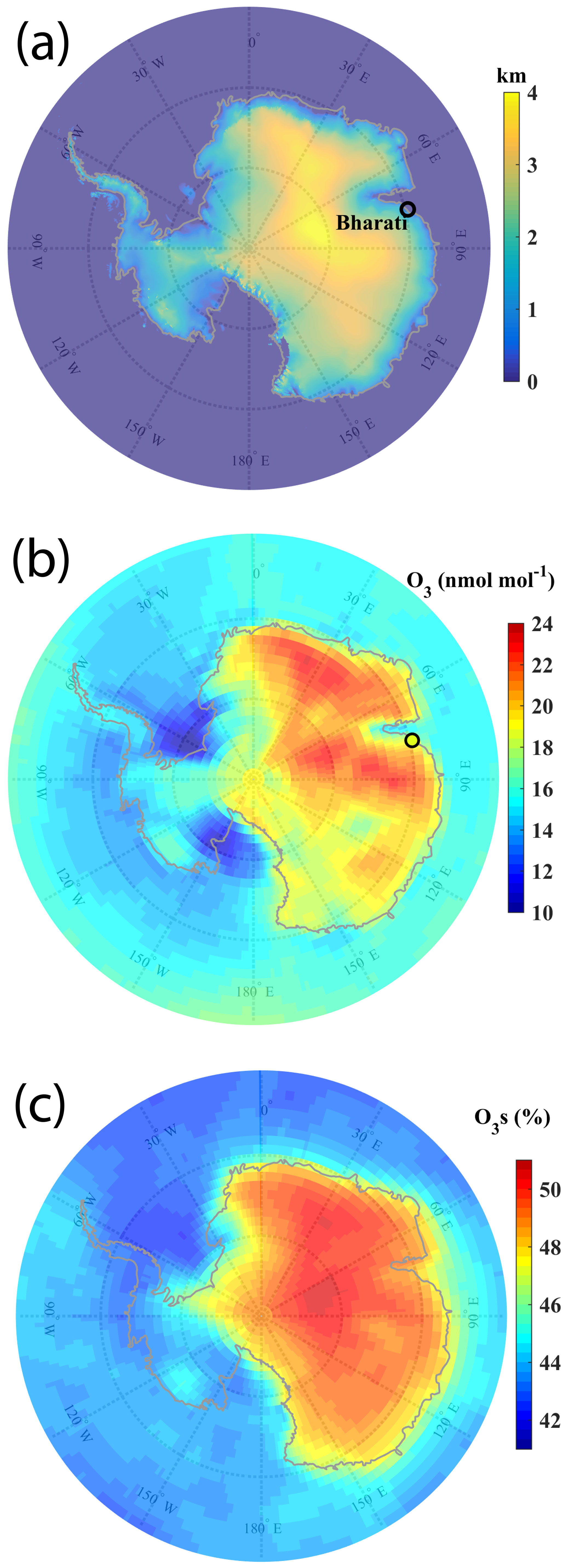
Figure 1(a) Elevation map of Antarctica, along with the location of the Indian station Bharati marked by a black circle. (b) Spatial distribution of surface O3 simulated by the EMAC model, averaged over the study period (29 January–13 February 2015, 17 January–24 February 2016, and 11 December 2016–16 February 2017). Colour in the black circle in (b) represents the mean value from the in situ measurements at Bharati. (c) Percent contribution of stratospheric O3 to the surface O3 derived from the EMAC model during the study period.
Figure 1c shows the stratospheric contribution (in percent) to the surface O3 based on the stratospheric O3 tracer in the model (O3s). O3s is seen to contribute 41 %–51 % over the Antarctic region, with greater contribution (45 %–51 %) over the continent with a higher elevation than that over the surrounding ocean (41 %–45 %). The mean stratospheric contribution at the observation site Bharati is estimated to be ∼ 48 % (∼ 10 nmol mol−1), showing that nearly half of O3 at the surface is of stratospheric origin. Mihalikova and Kirkwood (2013) have estimated a 6 %–7 % occurrence rate of tropospheric folds (one to two folds per month) during the summer using radar observations at Troll station (72.0∘ S, 2.5∘ E; 1275 m a.m.s.l.). In another recent study also, the enhancement by 20–30 nmol mol−1 (67 %–100 % as compared to the climatological mean) is seen in upper-tropospheric O3 above Bharati station due to stratospheric intrusions (Das et al., 2020). In addition, gradual subsidence through the tropopause also contribute to stratospheric O3 transport into the troposphere. Therefore, stratospheric intrusions are suggested to transport the O3-rich air masses to the troposphere, which subsequently descend to the surface and get redistributed across the region through horizontal transport. Descent of O3-rich air masses is further discussed in Sect. 3.2.
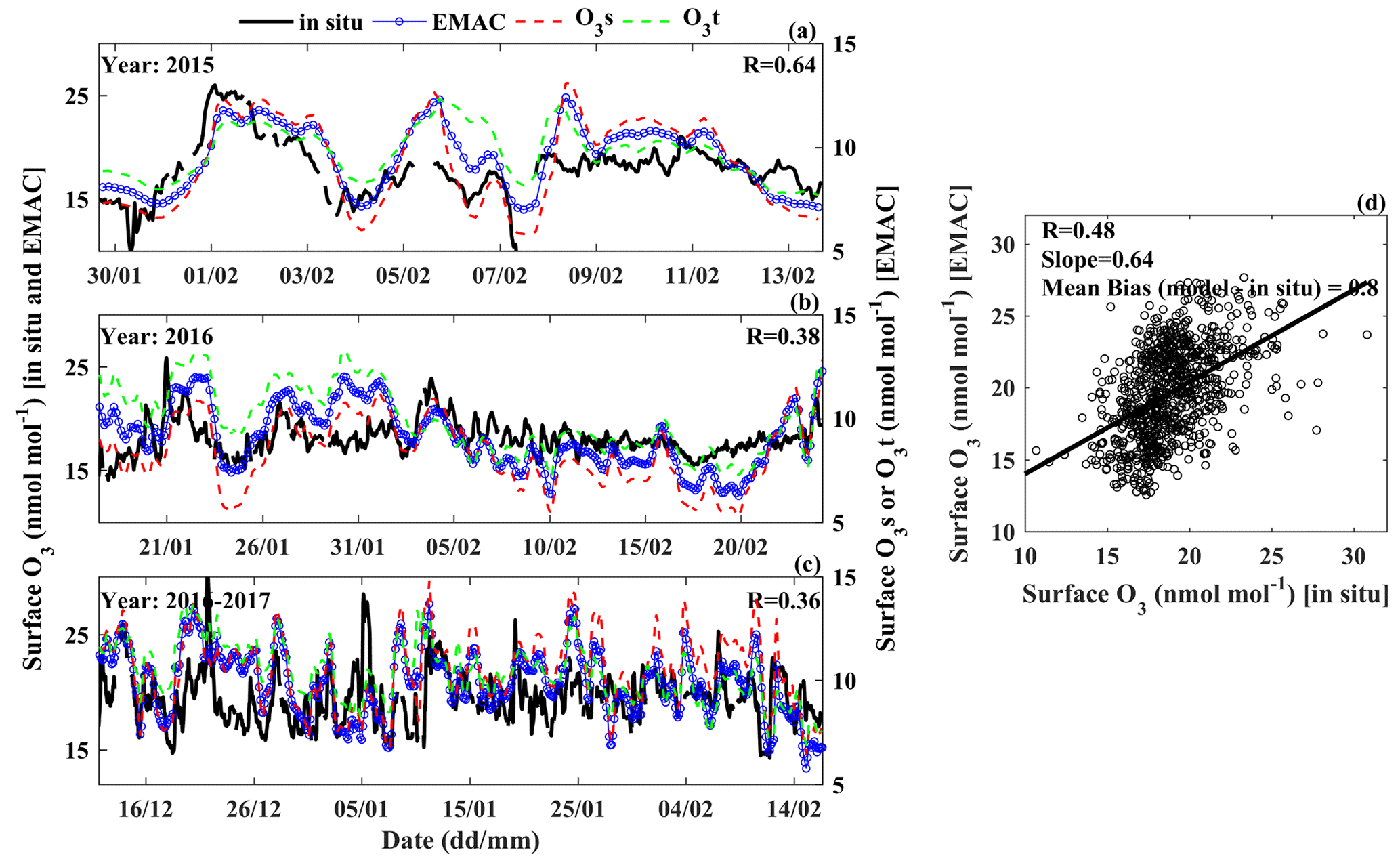
Figure 2Variability in surface O3 (a–c) at Bharati during austral summer of 2015–2017 based on in situ measurements (black) and EMAC simulations (blue). Green and red curves show the absolute stratospheric (O3s) and tropospheric (O3t) contributions to the surface O3. A scatter plot between in situ measurements and model-simulated O3 is shown in (d). Note that O3s and O3t are on a different scale on the right y axis in (a)–(c).
Figure 2a–c show the variations in surface O3 at Bharati station from in situ measurements and model simulations during the summer seasons of 2015–2017. The mean O3 levels estimated from the model simulations (19.7 ± 3.2 nmol mol−1) are in very good agreement with the measurements (18.8 ± 2.3), with negligible bias (∼ 1 nmol mol−1) at this station. Further, the surface O3 level at Bharati is observed to be similar to an earlier observation (∼ 13–20 nmol mol−1) at this station (Ali et al., 2017) and also to other stations in the coastal region of East Antarctica (Fig. S1). The model tends to successfully capture several features of the observed variability (Fig. 2a–c); nevertheless the overall correlation coefficient is 0.48 (Fig. 2d). The comparison for two other coastal stations, Syowa and Arrival Heights, during the same study period, also shows that the model can reproduce summertime O3 levels with small bias and the temporal variability moderately well (Figs. S2–S3). The blue and green curves in Fig. 2 show the individual contributions from stratospheric (O3s) and tropospheric sources (O3t = O3 − O3s), respectively. Both stratospheric and tropospheric sources are estimated to be contributing nearly equally, 48 % and 52 %, respectively. Further, the stratospheric O3 and tropospheric O3 at the surface are seen to be strongly correlated (R = 0.9; figure not shown) over most of the region, mainly due to the mixing of stratospheric and tropospheric air masses during the transport from the tropopause to the surface. Direct transport of stratospheric air or local O3 production would decrease the correlation or perturb the variations in O3s and O3t. Overall, similar variability of comparable magnitude in O3s and O3t indicates the absence of strong “local” production or “direct” stratospheric transport to the surface. However, about 50 % of the stratospheric contribution to surface O3 points to significant stratospheric intrusions over the Antarctic region.
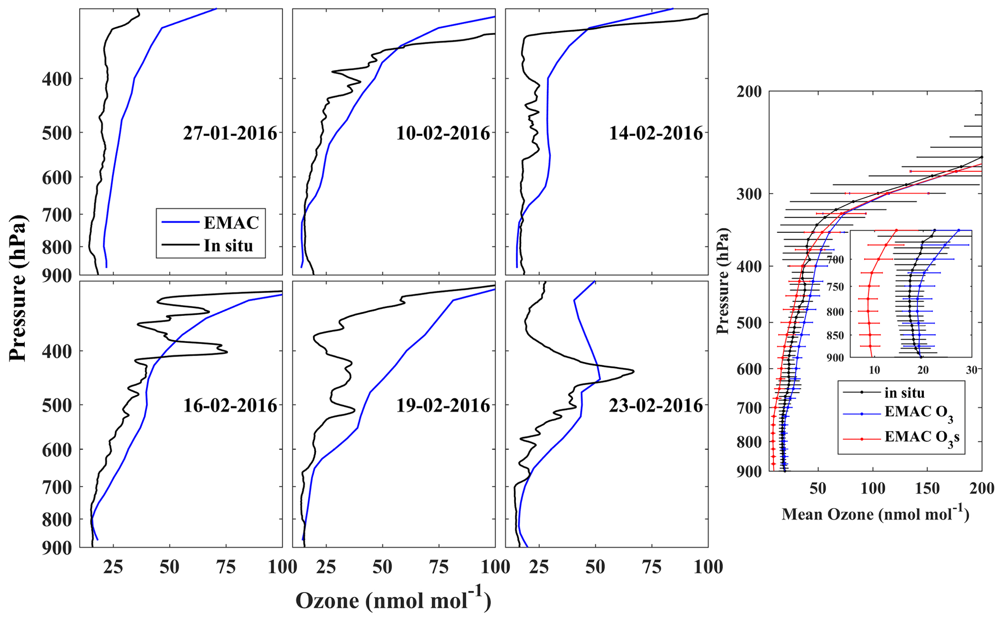
Figure 3Vertical profiles of O3 over Bharati station during a few representative days, based on the in situ measurements (black) and EMAC simulation (blue). The insert on the right shows the mean vertical distribution of O3 and O3s (red) corresponding to 12 profiles during the study period.
Figure 3 shows the comparison of balloon-borne observations of O3 vertical profiles with model simulation over Bharati station in 2016. Out of 12, 6 individual representative profiles are shown in the figure. O3 mixing ratios gradually increase with altitude up to the tropopause (∼ 8.5 km; ∼ 300 hPa), also showing O3 peaks in the middle/upper troposphere during some days. The model successfully captures the mean vertical distribution, especially in the lower troposphere (pressure > ∼ 700 hPa), with a mean bias of less than 2 nmol mol−1. There is an agreement between the model and observations in the upper troposphere; however, the model overestimates O3 levels (by ∼ 12 nmol mol−1) at the tropopause. Ozonesonde measurements from another station in the region, Davis (68.6∘ S, 78.0∘ E), were also compared with the model results for the study period (Figs. S4 and S5). The O3 variability from model results (standard deviation: 3–13 nmol mol−1) is comparable or slightly lower than the observed variability in the vertical distribution (950–350 hPa). The O3s contribution is ∼ 45 %–50 % in the lower troposphere (pressure > ∼ 700 hPa) but increases with altitude to 65 % at 500 hPa up to 100 % at and above the tropopause (∼ 300 hPa). The EMAC model captures both the mean vertical structure and some secondary O3 peaks (e.g. 23 February 2016; Fig. 3) in the upper troposphere (∼ 6 km; 450 hPa). However, there are some noticeable differences between the model and observations on individual days (e.g. 19 February 2016; Fig. 3). The model limitations in reproducing some features of secondary peaks have been suggested to be due to coarser vertical resolution and the temporal differences (Ojha et al., 2017) and were confirmed recently in a study focusing on tropopause folding frequency (Bartusek et al., 2023).
Overall, the model reproduces the observed tropospheric O3 distribution and most of the day-to-day variability in the surface and tropospheric O3. It is to be noted that the performance of global chemistry–climate models is also limited by the parameterisation schemes developed for such pristine environments with extreme climatic conditions (e.g. frequent blizzards). Note that depletion of surface O3 was observed over Antarctica during blizzards as blowing snow, which is a source of sea salt aerosols and subsequently bromine, which could deplete O3 (Jones et al., 2009; Ali et al., 2017). Nevertheless, our study fills a gap with respect to the evaluation of the widely applied EMAC model for the Antarctic region, and the results may have implications for further improving the model in future studies.
3.2 Influences of downward transport on surface O3
Several events of surface O3 enhancements were observed during the study period, as illustrated in Fig. 2. Two such events on 23 February 2016 and 1 February 2015 are investigated in detail to understand the mechanism driving such variability.
Figure 4a shows that surface O3 over Bharati was enhanced sharply by ∼ 4 nmol mol−1 around 23:00 local time (LT; which is UTC+5) on 23 February 2016. Backward air mass trajectories show that this air mass originated from ∼ 3 km altitude about 12 h before the event. The balloon-borne O3 vertical profile obtained at that time (11:00 LT on 23 February 2016; Fig. 4b) shows the presence of a layer with enhanced O3 (∼ 22 nmol mol−1) relative to lower altitudes (∼ 15 nmol mol−1). Based on these collocated observations and trajectory simulations, it is suggested that the O3-rich air from this layer descended to the surface over Bharati in ∼ 12 h with a descent rate of > 250 m h−1 (0.07 m s−1). The estimated descent velocity seems to be consistent with the in situ-measured mean vertical wind speed (0.09 ± 0.29 m s−1) measured at this station during 18–29 January 2016. The O3 enhancement observed in the upper troposphere (∼ 6 km; see Fig. 3) on 23 February 2016 is associated with a stratospheric intrusion (Das et al., 2020). The presence of the jet-stream in the vicinity of the tropopause (∼ 9 km altitude; ∼ 300 hPa) can enhance the turbulence due to strong wind shear (squared wind shear = 5 × 10⁻⁴ s−2). Along with this turbulence, tropopause oscillations led to the stratospheric intrusion during 22–23 February 2016 (Das et al., 2020). The presence of similar surface O3 enhancement events on several other days also (Fig. 2) suggests that this is a periodic phenomenon that significantly contributes to tropospheric O3 in the region.
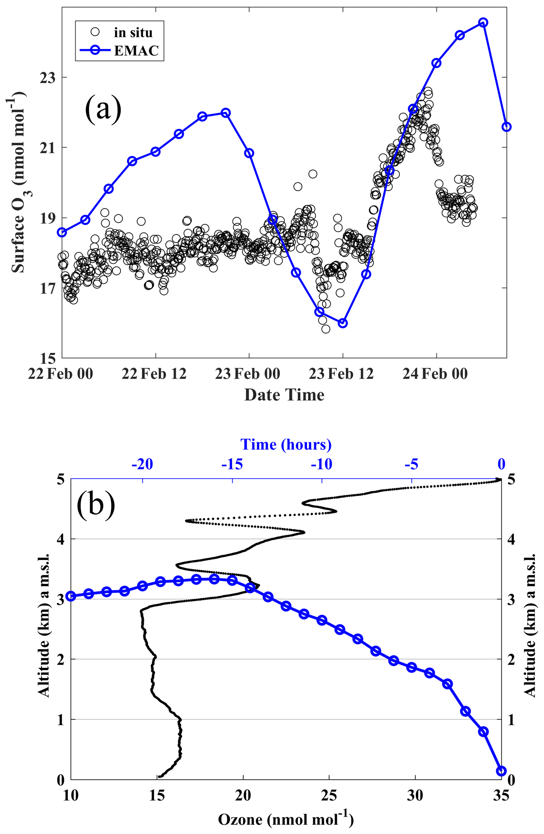
Figure 4(a) Surface O3 variations at Bharati station depicting an event of significant O3 enhancement around 23:00 LT on 23 February 2016. (b) Variations in the altitude of air mass (blue) along the backward trajectory with respect to time from the O3 enhancement event. Vertical profile of O3 measured around 11:00 LT on 23 February 2016 (black).
Surface O3 shows a continuous enhancement from about 12–14 nmol mol−1 on 31 January 2015 to about 25 nmol mol−1 on 1 February 2015 (Fig. 2a). To analyse the influence of transport from the stratosphere, the spatial distribution of the stratospheric O3 tracer at different pressure levels is combined with air mass trajectories (Fig. 5). The insert in Fig. 5a shows a zoomed-in view of O3s around Bharati station on 1 February 2015. The air mass backward trajectory ending at Bharati station at the time of the observed enhancement is shown by the black curve. The air mass is traced back to ∼ 600 hPa (∼ 4 km) 1 d prior to the observed enhancement (i.e. 31 January 2015) at a lower latitude, where a patch of stratospheric O3 (20 nmol mol−1) is simulated by the model. A clear descent of air mass with a descent rate of ∼ 0.05 m s−1 is seen, leading to the enhancement in surface O3 on 1 February 2015.
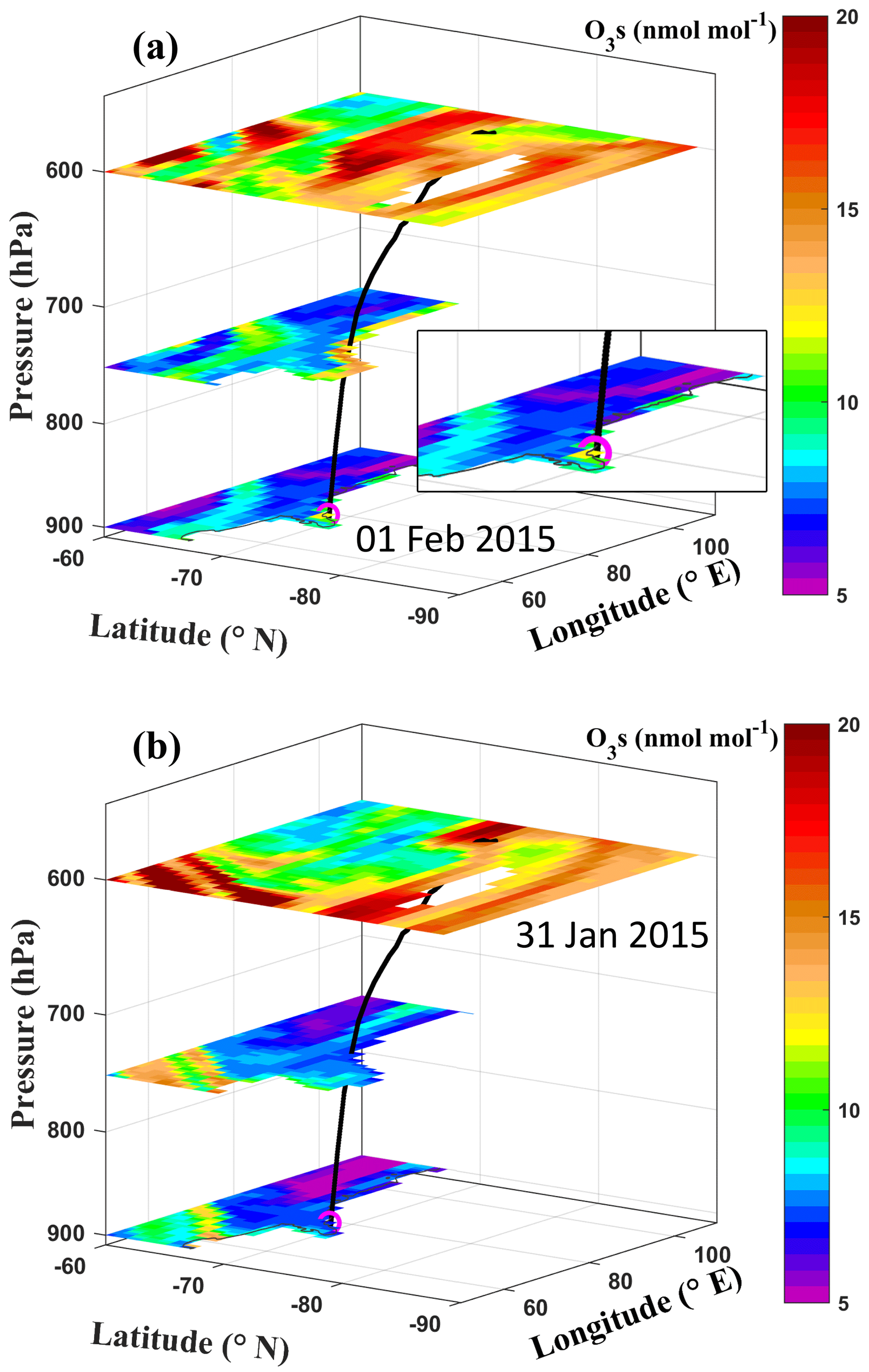
Figure 5Spatial distribution of the stratospheric O3 tracer in the model at different pressure levels for (a) 1 February 2015, depicting an enhancement at the surface, and (b) 31 January 2015, depicting an enhancement in the upper troposphere. The black curve represents a 24 h backward air mass trajectory ending at Bharati station (magenta circle) on 1 February 2015 and originating around 600 hPa on 31 January 2015.
The above analysis of two representative events shows that the intrusion of stratospheric O3 followed by descent of O3-rich air can cause a 4–10 nmol mol−1 enhancement in surface O3 during the study period. The result is in line with a continuous increase in O3 and O3s with altitude, as shown in Figs. 1c and 3. Similar variations of O3t compared to O3s (Fig. 2) indicate significant air mass mixing during the transport process. O3 enhancement events with similar magnitude were also observed at the nearby station Zhongshan (69.37∘ S 76.36∘ E; Ding et al., 2020; Tian et al., 2022) and with larger magnitude at the South Pole (8–20 nmol mol−1; Oltmans et al., 2008), attributed to transport- or NOx-driven cumulative photochemical production, assuming a marginal role of transport from the stratosphere or free troposphere (Cristofanelli et al., 2018; Ding et al., 2020). The occurrence of such O3 enhancement is less evident over the coastal regions compared to the Antarctic Plateau (Jones, 2003). However, substantial contributions of stratosphere-troposphere exchange were associated with air mass fluxes up to 60 kg m−2 d−1 (Sanak et al., 1985) using in situ measurement of beryllium isotope at Dumont d'Urville station. Based on long-term balloon-borne measurements and GOES-Chem (Goddard Earth Observing System coupled with Chemistry) model simulations, Greenslade et al. (2017) also reported large stratosphere–troposphere O3 fluxes (0.50–0.75 × 10¹⁷ molecules cm−2 per month) during the summer, which exceed those during the winter (0.25–0.50 × 10¹⁷ molecules cm−2 per month).
3.3 Influences of photochemistry on surface O3
The production and loss rates of O3 through different chemical pathways have been estimated from the EMAC model simulation, and the mean values during the study period are shown in Fig. 6a. Among various production and loss reactions, O3 + HO2 and H2O + O(1D) are found to be the dominant O3 loss pathways, whereas NO + HO2 and NO + CH3O2 are the major O3 production reactions. Overall, the aforementioned chemical losses tend to dominate the production leading to a net photochemical loss in surface O3 at Bharati. Effectively the study region acts as a net chemical sink of O3. Note that loss through O3 + OH and other reactions and production through NO + RO2 and other reactions are relatively small in magnitude (Fig. 6). Dry deposition over ice and the surrounding ocean is a minor O3 removal mechanism as well. The substantial variability (large error bars in Fig. 6a) in production and loss terms arises from the diurnal and day-to-day variations. Figure 6b–c show the mean diurnal variation of net photochemical production or loss rates from the EMAC model and the rate of change of O3 (i.e. ) from in situ measurements. The net loss is relatively high during noontime (11:00–14:00 LT) and negligibly small after 23:00 LT and prior to 05:00 LT. In situ-measured rate of change, , is negative around 11:00 LT, indicating overall loss, which includes the influences of both photochemistry and dynamics and deposition losses. Since the mean amplitude of in Fig. 6c is 0.3 nmol mol−1 h−1, which is comparable to or smaller than the variability at any given hour of the day, diurnal patterns on different days might vary from the mean picture. The positive rate of change after 17:00 LT and prior to 05:00 LT represents an increase in O3 mainly through horizontal or vertical transport as photochemistry is weak under conditions of low solar irradiance.
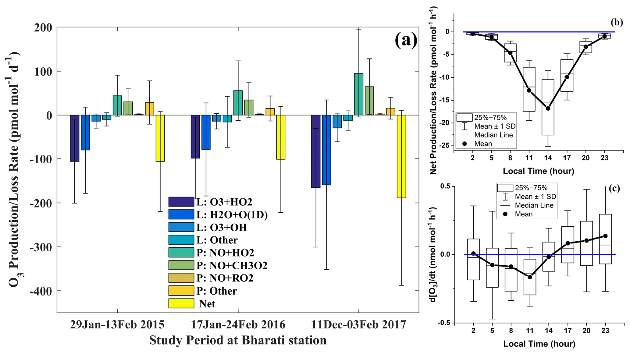
Figure 6(a) Mean production and loss rates of surface O3 through different chemical pathways at Bharati during the study period; (b) diurnal variation of net O3 change due to photochemistry, derived from the EMAC model simulations; and (c) rate of change of surface O3 () based on the in situ measurements at Bharati station.
Despite being a net photochemical sink of surface O3, it is observed that the levels of O3 are relatively steady or continuous over time (Fig. 2c). We estimated surface O3 fluxes by multiplying the model-simulated vertical wind by the O3 concentration at the model level just above the surface. Figure 7b shows the mean O3 flux averaged over the study period. The negative flux represents the number of O3 molecules moving downward (contributing to surface O3) per unit area and per unit of time. A stronger downward flux along the east coast (Fig. 7b) counterbalances the net photochemical O3 loss (Fig. 7a). Assuming a boundary layer height of 500 m, the loss rates integrated over boundary layer are estimated at 2.7 × 10¹³ molecules m−2 s−1, which is of comparable magnitude to the modelled downward flux (Fig. 7b). O3 and O3 fluxes (i.e. fluxes at level just above the surface) correlate negatively (R = −0.3) at Bharati in the EMAC simulation, as shown in Fig. S6a. This is substantiated with a negative correlation of surface O3 with the vertical wind (Fig. S6b), suggesting enhanced O3 during conditions of descent. The results suggest that despite the net chemical sink of O3, the surface O3 is maintained by a flux from above during the summer over the coastal region. The O3 loss through chemistry is counterbalanced by the contribution from dynamics (or vice versa) over East Antarctica during austral summer.
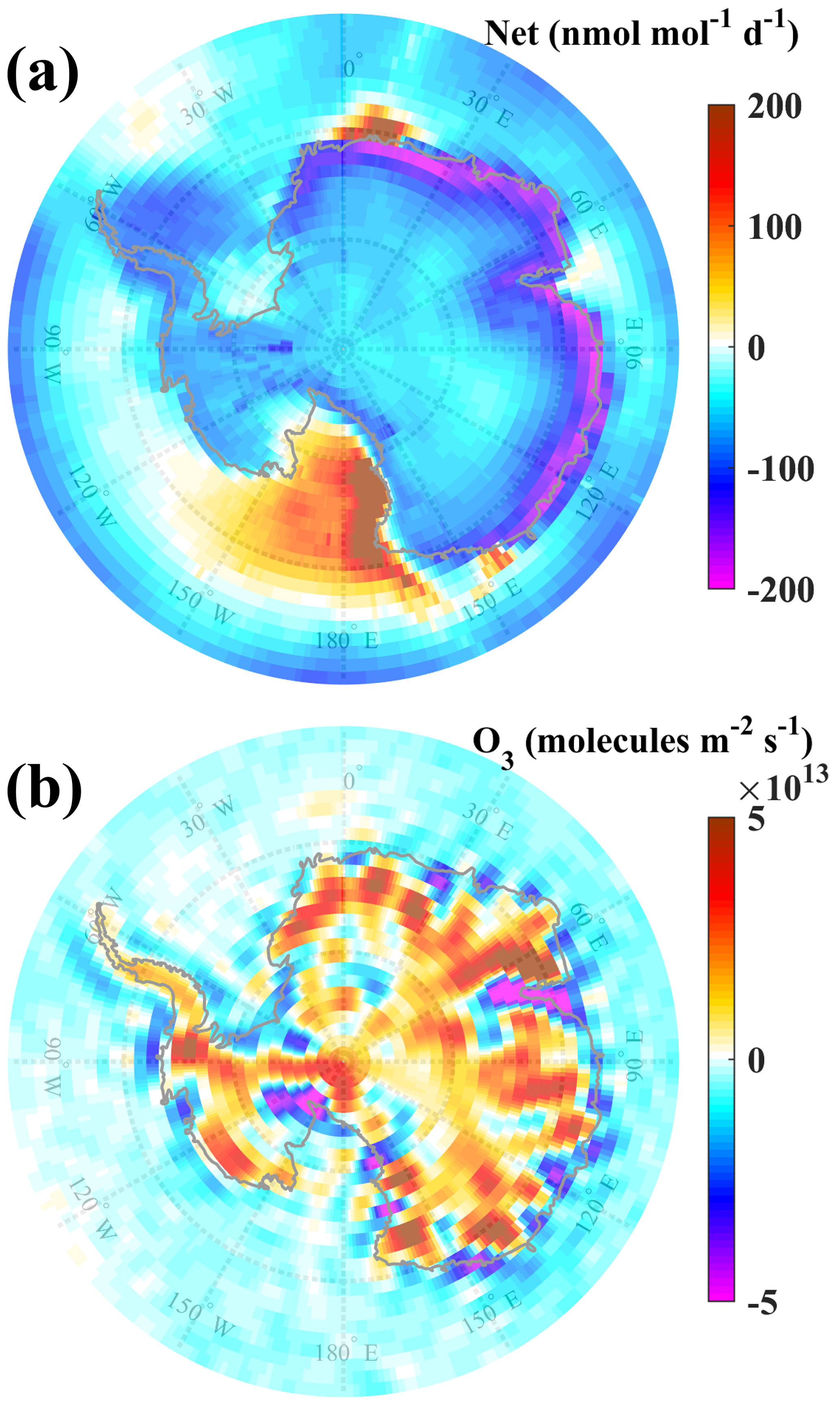
Figure 7Spatial distribution of (a) net rate of change (production minus loss) of surface O3 due to photochemistry and (b) O3 flux at surface averaged over the study period.
In order to understand whether the O3 photochemical loss over the Bharati station also prevails over larger regions in Antarctica, we analyse the spatial distribution of net production or loss rates averaged during the austral summer (Fig. 7a). It is important to note that our simulations show that the entire Antarctic continent acts as a sink of O3, in contrast to the previously reported net O3 production through NO emission from snow (Legrand et al., 2016 and references therein). In the east coastal Antarctic region O3 loss rates are significantly higher (∼ 190 pmol mol−1 d−1), suggesting that it acts as a relatively strong chemical sink of surface O3. The loss rate is at a peak (∼ 190 pmol mol−1 d−1) over the east coast, higher by ∼ 100 pmol mol−1 d−1 compared to adjacent land and ocean, and it gets further lower (∼ 50 pmol mol−1 d−1) much away from the coast. Note that model-simulated mean OH and NO are in the range of 0.05–0.5 × 10⁶ molecules cm−3 and 0.5–10 pmol mol−1, respectively, over the entire Antarctic region, which is in line with earlier measurements at the west coast (OH mean – 0.11 × 10⁶ molecules cm−3, ranging < 0.1–0.9 × 10⁶ molecules cm−3; NO – estimated value of 5 pmol mol−1) by Jefferson et al. (1998) and Bloss et al. (2010) but lower (almost 5 times) than those measured during the OPALE campaign (OH mean – 2.1 × 10⁶ molecules cm−3, ranging < 0.8–6.2 × 10⁶ molecules cm−3; NO – 5–70 pmol mol−1; Kukui et al., 2012).
The net O3 loss rate (Fig. 7a) is found to be lower over land than over ocean and is highest along the east coast. We further considered six grids on both sides of the coastline and averaged over the longitude range 15–130∘ E (i.e. East Antarctica). The variations in average production and the loss and net rates with latitude are shown in Fig. 8. Since the latitudes corresponding to different grids at 15–130∘ E are different, latitudes shown on the x axis represent average latitudes. Thus, as we proceed from left to right (lower latitude to higher latitude) in Fig. 8, we move from land to ocean.
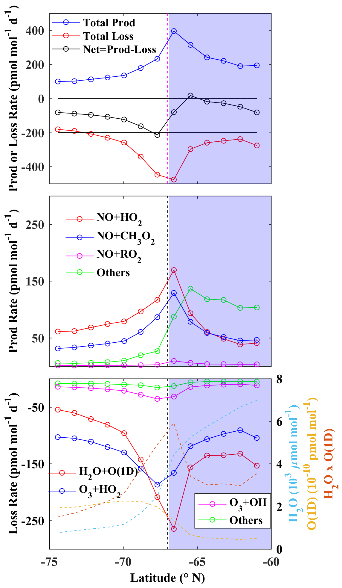
Figure 8Latitudinal variation of production and loss and net rates of changes of surface O3 averaged along the east coastal longitudinal band of 15–130∘ E during January 2017. The blue areas represent the ocean environment, and the vertical dashed line shows the approximate coastline.
From Fig. 8a, it is clearly seen that the O3 production, as well as loss, is maximum near the coast. Since loss dominates over the production, the net rate is negative, with ∼ 190 pmol mol−1 d−1. Figure 8b and c represent changes in different production and loss pathways across the coast. The photolytic O3 loss, followed by H2O + O(1D), is found to be the dominating loss process, peaking at ∼ 300 pmol mol−1 d−1 along the coast. The reason for the peak loss rate at the coast is related to the opposite latitudinal gradients in H2O and O(1D) (see Fig. 8c; right axis). H2O is substantially higher (∼ 6000 µmol mol−1) over ocean but much lower (1000 µmol mol−1) in the drier atmosphere above the continent. In contrast, O(1D) is higher (2 × 10⁻¹⁰ pmol mol−1) over the continent, primarily due to intense solar insolation at higher elevation and over the bright ice surface. Therefore, latitudinally opposite variations of H2O and O(1D) lead to a relative maximum in H2O + O(1D) near the coast. We also note that there is significant O3 production over the ocean due to reactions other than the three primary reactions of peroxy radicals (HO2, RO2, CH3O2) with NO.
Thus, under the prevailing relatively strong O3 sink along the east coast, the mean O3 level during the summer is maintained by the downward flux of O3 from the stratosphere.
3.4 Diurnal variation of surface O3 at Bharati
Considering day-to-day variability, including enhancement events governed by stratospheric influence, ΔO3 is computed by subtracting the running mean O3 (288 points; 5 min interval – daily running mean) from the observed O3. Figure 9a shows the mean diurnal variation of ΔO3 during the 18 January–23 February 2016 period for which measurements of horizontal wind at surface were also available. Surface O3 exhibits a diurnal variation, being relatively low during the afternoon (15:00 LT) and relatively high during nighttime (Fig. 9), with a diurnal amplitude of ∼ 1.2 nmol mol−1. Figure 9b shows the wind rose colour coded with ΔO3 mixing ratios. Sunlight at Bharati is abundant during the summer, and the land–sea thermal contrast explains the typical diurnal change in the wind direction under normal meteorological conditions, i.e. excluding blizzards and snowstorms. Figure S7 shows time series of the wind direction and surface ΔO3, depicting the link between O3 and the wind direction. Due to higher O3 over the eastern Antarctic land regions, winds from that sector transport the O3-rich air to the Bharati station, causing enhanced O3 mixing ratios. O3 is higher when wind is parallel to the coast (easterly; wind direction ∼ 90∘) or from the land (wind direction: 90–240∘). Under calm wind conditions, the influence of transport is minimal, and photochemical loss is more pronounced. When the wind is weak and from the ocean (wind direction: 30–90∘ N), O3 levels are lower due to dilution by mixing with air from the oceanic sector. The O3 diurnal variation is also closely linked with the vertical wind. Based on limited in situ measurements of the vertical wind at the surface during 18–29 January 2016, the mean diurnal variation of vertical wind (w) along with ΔO3 is shown in Fig. 9c. Downdrafts and stronger updrafts (up to ∼ 0.4 m s−1) are seen during nighttime (or lower solar zenith angle; 20:00–07:00 LT) and daytime (08:00–19:00 LT), respectively. Higher O3 during nighttime is associated with downdrafts, and O3 mixing ratios are reduced with increasing updraft intensity. The EMAC model shows limitations in reproducing the observed diurnal variation, likely because of coarse resolution averaging out the topography and mesoscale dynamics.
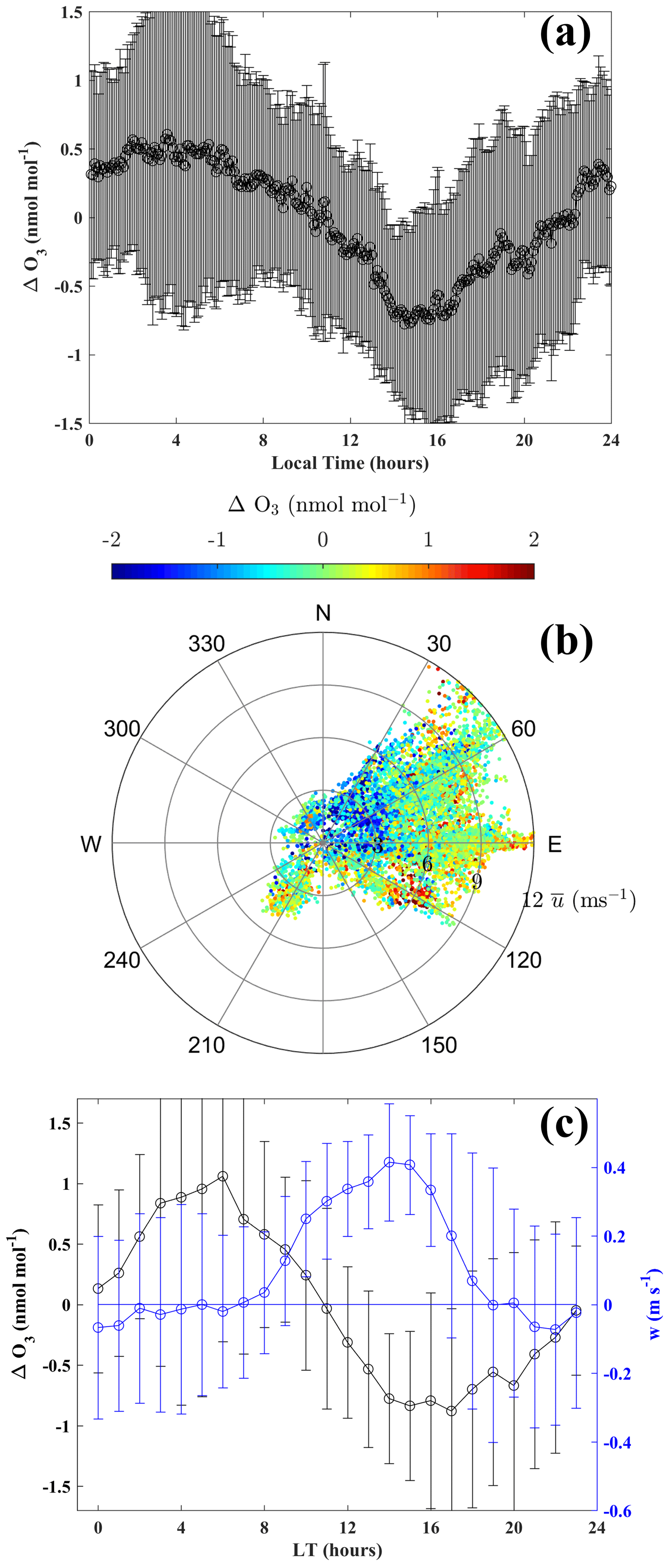
Figure 9(a) Diurnal variation of ΔO3, (b) wind rose colour coded with ΔO3, and (c) variation in collocated vertical wind and ΔO3 at Bharati during the austral summer of 2016.
Diurnal patterns with an amplitude ranging from ∼ 0.2–2 nmol mol−1 were reported at coastal (Syowa and McMurdo) and inland (Concordia; 75∘ S; 123∘ E; 3220 m above sea level) stations (Ghude et al., 2006; Legrand et al., 2009). However, such a pattern is absent over the South Pole (Oltmans, 1981). Interestingly, photochemical production during the morning hours (05:00–11:00 LT) due to the NOx released from snow was followed by a reduction due to an increase in boundary layer height (200 ± 100 m) at the inland station Concordia (Legrand et al., 2009, 2016). Shallow convective boundary layers (less than 300 m) were reported over the Antarctic Plateau region by Mastrantonio et al. (1999). Unlike these studies, we did not observe photochemical O3 production, nor a clear signature of changes in O3 transport across the top of boundary layer from our ozonesonde measured O3 profiles over Bharati station. Therefore, the diurnal patterns of O3 over coastal Antarctica are found to be different than those over the inland region, mainly due to differences in meteorological conditions and the concentrations of precursor gases.
3.5 Absence of signature of halogen chemistry
Reactive halogens (e.g. iodine, bromine) have been shown to deplete O3 in the boundary layer over the Antarctic region (Barrie et al., 1988; Oltmans and Komhyr, 1976). However, ground-based remote sensing observations found very low concentrations of iodine oxide (∼ 0.3 ± 0.1 pmol mol−1) in the boundary layer over Bharati station during the study period (Mahajan et al., 2021), and no clear sign of O3 depletion was observed.
Satellite (SCIAMACHY – SCanning Imaging Absorption spectroMeter for Atmospheric CartograpHY and OMI – Ozone Monitoring Instrument) observations also show lower monthly mean iodine monoxide (IO) columnar density (0–1 × 10¹² molecules cm−2) over Bharati compared to West Antarctica (figure not shown). This is consistent with previous studies (e.g. Schönhardt et al., 2012) showing relatively low IO over East Antarctica and the adjacent ocean (≤ 0.7 × 10¹² molecules cm−2) compared to West Antarctica (∼ 1.5 × 10¹² molecules cm−2) during the summer season (December–January–February 2004–2009).
Bromine (Br)-driven O3 depletion events, resulting in BrO, are less frequent over the Antarctic region compared to the Arctic region due to differences in springtime surface temperatures (Tarasick and Bottenheim, 2002). However, large O3 depletion events were observed at Neumayer (70.62∘ S, 8.37∘ W; 42 m a.m.s.l.) during the late winter (July to September), likely due to stronger BrO episodes from the larger sea ice coverage around the site (Legrand et al., 2009). Analysis of BrO from OMI possibly indicates an O3 depletion event on 7 February 2015 at Bharati where BrO was enhanced, ∼ 9.2 × 10¹³ molecules cm−2 with lower O3 (∼ 7 nmol mol−1), marked by the red rectangle in Fig. S8. Except for this event, BrO remained below 8 × 10¹³ molecules cm−2 around Bharati station (±0.5∘ latitude/longitude) during the study. O3 depletion was also not seen at Syowa (Fig. S9) during the study period. The coastal region of East Antarctica exhibits slightly higher values of BrO (∼ 7 × 10¹³ molecules cm−2) compared to the ocean and land regions (4–6 × 10¹³ molecules cm−2). However, it is low (4–8 × 10¹³ molecules cm−2) during December–February (2004–2009) compared to the levels during September–November (5–10 × 1013 molecules cm−2) over the Antarctic region (Schönhardt et al., 2012). The impact of Br chemistry on surface O3 is suggested to be weaker along the east coast of Antarctica (Dumont d'Urville and Syowa) in contrast to western coastal Antarctica, as observed over the Neumayer and Halley (75.55∘ S, 26.53∘ W; 30 m a.m.s.l.) stations (Legrand et al., 2016). Nevertheless, simultaneous measurements of O3 and halogen species including BrO are desirable to quantify the role of halogen chemistry over eastern Antarctica.
3.6 Surface O3 during the winter
To take into account the seasonality of O3 at the surface, the wintertime distribution is shown in Fig. S10. The mean surface O3 level is higher during the winter (20–32 nmol mol−1) compared to the summer (11–23 nmol mol−1), in line with the reported seasonality in the literature (Legrand et al., 2009). Figure S10 reveals three low-O3 patches over the coastal oceanic region. One is close to Bharati station; however, we do not have observations during the wintertime for comparison. Model simulations suggest that surface O3 is composed of 63 %–67 % O3s of stratospheric origin during the winter (Fig. S10b), which is significantly higher than during austral summer. The probability of downward transport from the stratosphere during the winter, also associated with a lower altitude of the tropopause, is larger (Kumar et al., 2021). Comparison of surface O3 at Syowa (69.00 ∘ S; 39.58 ∘ E; not shown here) shows that the model captures the variability with R = 0.3 and a negative bias of ∼ 5 nmol mol−1. The model performance seems to be better during the summer, indicative of limitations to reproduce the mean O3 concentrations and the variability during the winter. Further studies are needed to understand and rectify the factors causing greater bias in the model during the winter. Analysis of the O3 budget suggests a small net loss of O3 by 10–25 pmol mol−1 d−1 over the oceanic region and close to zero (< 5 pmol mol−1 d−1) over the Antarctic continent (Fig. S11). To study this in greater detail, we highly recommend conducting continuous wintertime measurements of O3 and its precursors including halogens over Bharati during the winter season.
Ground-based and balloon-borne O3 measurements have been conducted over the Indian station Bharati on the east coast of Antarctica during the austral summers of 2015–2017. The observations have been used to evaluate the performance of the global chemistry–climate model EMAC over this part of the world. A comprehensive analysis of observations and model simulations provided significant insights into the dynamical and photochemical processes affecting surface O3 and its variability. The main results are as follows:
-
Surface O3 levels over the Indian station Bharati in eastern coastal Antarctica have been observed to be ∼ 19 nmol mol−1 with a small variability of ∼ 2 nmol mol−1 during austral summer. While similar levels prevail over the east coast, O3 is typically higher over land at higher elevation. The EMAC model successfully reproduced the observed mean levels with negligible bias over this unique environment and also captured the temporal variability (R = 0.5). In particular, the model successfully reproduced some events during which O3 was enhanced. Analysis of the stratospheric O3 tracer in the model suggests that 41 %–51 % of surface O3 is of stratospheric origin, with larger fractions over the higher-elevation regions in Antarctica.
-
The model successfully reproduced the mean vertical distribution of O3 over Bharati observed by balloon-borne soundings. Detailed analysis combining the balloon profiles, model tracers, and air mass trajectories shows that downward transport caused the observed events during which O3 was enhanced.
-
Along the east coast of Antarctica, including Bharati station, photochemistry acts as a relatively strong sink of surface O3 (∼ 190 pmol mol−1 d−1) when compared to adjacent land and ocean regions. Chemical loss through O3 photolysis (followed by H2O + O(1D)) and O3 + HO2 dominates over the major production (through NO+HO2 and NO+CH3O2). Reverse latitudinal gradients between H2O and O(1D) lead to maximum O3 loss at the coastal region. The continuous chemical loss is found to be counterbalanced by downward O3 transport from above. The findings show the intertwined roles of dynamics and photochemistry that govern the O3 variability over East Antarctica and how significant O3 levels are maintained despite the absence of local precursor sources.
-
In addition to the role of photochemistry, the diurnal variation of O3 at Bharati was found to correlate with the diurnal wind changes. Surface O3 varied with a diurnal amplitude of 1.2 nmol mol−1, with the higher levels occurring when the wind blew parallel to the coast or from land regions. In addition, up- and downdrafts also play a role in the diurnal variation.
Our observations during austral summer over 3 years complement available data, for example, from eastern coastal Antarctica. The observations, besides revealing diurnal and day-to-day variability, helped in evaluating the performance of a global chemistry–climate model over this unique, pristine environment. The study provides valuable insights into the complementary roles of photochemistry and dynamics in governing O3 and its variability over Antarctica. In view of increasing anthropogenic activities and the changing climate, monitoring of O3 and related species (NO, NO2, CO, VOCs, and halogens) is needed.
The Modular Earth Submodel System (MESSy) is continuously further developed and applied by a consortium of institutions. The usage of MESSy and access to the source code is licensed to all affiliates of institutions that are members of the MESSy Consortium. Institutions can become a member of the MESSy Consortium by signing the MESSy Memorandum of Understanding. More information can be found on the MESSy Consortium website (http://www.messy-interface.org, last access: 4 July 2023). The code presented here has been based on MESSy version 2.55 and is available as git commit #a5bd54d5b in the MESSy repository.
Measured ozone and EMAC-simulated fields shown in the figures can be obtained from the website of the Space Physics Laboratory (https://spl.gov.in/SPLv2/index.php/spl-metadata/104-spl/550-trace-gases-metadata.html, last access: 1 January 2024) or via a direct link, https://spl.gov.in/SPLv2/images/SPL-METADATA/Girach_et_al_2024_ACP_Ozone_Bharati_Antarctica.xlsx (last access: 1 January 2024; Girach and Pozzer, 2023). Surface ozone observations at Antarctic stations (South Pole, United States; Arrival Heights, New Zealand; Marambio, Argentina; Syowa, Japan) were obtained from the newly established World Data Centre for Reactive Gases (WDCRG), under WMO's GAW (Global Atmosphere Watch; World Meteorological Organization) programme (https://ebas-data.nilu.no/Default.aspx, last access: 1 January 2024; World Data Centre for Reactive Gases, 2023). Vertical O3 profiles measured at Davis station were obtained from https://woudc.org/data/explore.php (last access: 1 January 2024; Australian Bureau of Meteorology, 2023).
The supplement related to this article is available online at: https://doi.org/10.5194/acp-24-1979-2024-supplement.
IAG conceptualised and designed the study, performed measurements and analysed the datasets. KVS, NK, MMN, and NKK contributed in the measurements. AP performed the model simulations. NO, AP, PRN, SNSB, and JL helped IAG with the analysis and interpretation of the results. IAG wrote the manuscript, and all the co-authors contributed to the review and editing.
At least one of the (co-)authors is a member of the editorial board of Atmospheric Chemistry and Physics. The peer-review process was guided by an independent editor, and the authors also have no other competing interests to declare.
Publisher’s note: Copernicus Publications remains neutral with regard to jurisdictional claims made in the text, published maps, institutional affiliations, or any other geographical representation in this paper. While Copernicus Publications makes every effort to include appropriate place names, the final responsibility lies with the authors.
We gratefully acknowledge the organiser, Centre for Polar and Ocean Research (NCPOR), Goa, Ministry of Earth Sciences, India for providing the opportunity to participate in the 34th, 35th, and 36th Indian Scientific Expedition to Antarctica (ISEA). We also acknowledge the leaders of the Bharati station and voyage for providing necessary support for the smooth conduct of experiments at Bharati station. We are really thankful to Santosh Muralidharan, from the Space Physics Laboratory, and Brijesh Desai, in charge of the laboratory at Bharati station during the 35th expedition, and other expedition members of 34th, 35th, and 36th ISEA for their help during the field measurements. We also thank Mriganka Sekhar Biswas, Indian Institute of Tropical Meteorology, India, for fruitful discussion on halogen chemistry. We are also thankful to the India Meteorological Department (IMD) for providing meteorological observations and hydrogen gas cylinders for balloon ascents and for the help during balloon launches. The EMAC model simulations were performed at the German Climate Computing Centre (DKRZ). We highly acknowledge teams of researchers who made ozone measurements at various Antarctic stations and made them available publicly. We also acknowledge the NOAA Air Resources Laboratory (ARL) for the HYSPLIT transport and dispersion model used from their READY website (https://www.ready.noaa.gov/HYSPLIT.php, last access: 1 January 2024).
The article processing charges for this open-access publication were covered by the Max Planck Society.
This paper was edited by Jens-Uwe Grooß and reviewed by two anonymous referees.
Ajayakumar, R. S., Nair, P. R., Girach, I. A., Sunilkumar, S. V., Muhsin, M., and Chandran, P. S.: Dynamical nature of tropospheric ozone over a tropical location in Peninsular India: Role of transport and water vapour. Atmos. Environ.. 218, 117018, https://doi.org/10.1016/j.atmosenv.2019.117018, 2019.
Ali, K., Trivedi, D. K., and Sahu, S. K.: Surface ozone characterization at Larsemann Hills and Maitri, Antarctica, Sci. Total Environ., 584–585, 1130–1137, https://doi.org/10.1016/j.scitotenv.2017.01.173, 2017.
Australian Bureau of Meteorology: Ozonesonde, World Ozone and Ultraviolet Radiation Data Centre [data set], https://woudc.org/data/explore.php (last access: 1 January 2024), 2023.
Barrie, L. A., Bottenheim, J. W., Schnell, R. C., Crutzen, P. J., and Rasmussen, R. A.: Ozone destruction and photochemical reactions at polar sunrise in the lower Arctic atmosphere, Nature, 334, 138–141, https://doi.org/10.1038/334138a0, 1988.
Bartusek, S., Wu, Y., Ting, M., Zheng, C., Fiore, A., Sprenger, M., and Flemming, J.: Higher-Resolution Tropopause Folding Accounts for More Stratospheric Ozone Intrusions, Geophys. Res. Lett., 50, e2022GL101690, https://doi.org/10.1029/2022GL101690, 2023.
Bloss, W. J., Camredon, M., Lee, J. D., Heard, D. E., Plane, J. M. C., Saiz-Lopez, A., Bauguitte, S. J.-B., Salmon, R. A., and Jones, A. E.: Coupling of HOx, NOx and halogen chemistry in the antarctic boundary layer, Atmos. Chem. Phys., 10, 10187–10209, https://doi.org/10.5194/acp-10-10187-2010, 2010.
Bond, A. M. H., Frey, M. M., Kaiser, J., Kleffmann, J., Jones, A. E., and Squires, F. A.: Snowpack nitrate photolysis drives the summertime atmospheric nitrous acid (HONO) budget in coastal Antarctica, Atmos. Chem. Phys., 23, 5533–5550, https://doi.org/10.5194/acp-23-5533-2023, 2023.
Brühl, C., Schallock, J., Klingmüller, K., Robert, C., Bingen, C., Clarisse, L., Heckel, A., North, P., and Rieger, L.: Stratospheric aerosol radiative forcing simulated by the chemistry climate model EMAC using Aerosol CCI satellite data, Atmos. Chem. Phys., 18, 12845–12857, https://doi.org/10.5194/acp-18-12845-2018, 2018.
Crawford, J. H., Davis, D. D., Chen, G., Buhr, M., Oltmans, S., Weller, R., Mauldin, L., Eisele, F., Shetter, R., Lefer, B., Arimoto, R., and Hogan, A.: Evidence for photochemical production of ozone at the South Pole surface, Geophys. Res. Lett., 28, 3641–3644, https://doi.org/10.1029/2001GL013055, 2001.
Cristofanelli, P., Putero, D., Bonasoni, P., Busetto, M., Calzolari, F., Camporeale, G., Grigioni, P., Lupi, A., Petkov, B., Traversi, R., Udisti, R., and Vitale, V.: Analysis of multi-year near-surface ozone observations at the WMO/GAW “Concordia” station (75∘06′S, 123∘20′E, 3280 m a.s.l. – Antarctica), Atmos. Environ., 177, 54–63, https://doi.org/10.1016/j.atmosenv.2018.01.007, 2018.
Das, S. S., Ramkumar, G., Koushik, N., Murphy, D. J., Girach, I. A., Suneeth, K. V., Subrahmanyam, K. V., Soni, V. K., Kumar, V., and Nazeer, M.: Multiplatform observations of stratosphere-troposphere exchange over the Bharati (69.41∘ S, 76∘ E), Antarctica during ISEA-35, J. Atmos. Sol.-Terr. Phy., 211, 105455, https://doi.org/10.1016/j.jastp.2020.105455, 2020.
Davis, D. D., Eisele, F., Chen, G., Crawford, J., Huey, G., Tanner, D., Slusher, D., Mauldin, L., Oncley, S., Lenschow, D., Semmer, S., Shetter, R., Lefer, B., Arimoto, R., Hogan, A., Grube, P., Lazzara, M., Bandy, A., Thornton, D., Berresheim, H., Bingemer, H., Hutterli, M., McConnell, J., Bales, R., Dibb, J., Buhr, M., Park, J., McMurry, P., Swanson, A., Meinardi, S., and Blake, D.: An overview of ISCAT 2000, Atmos. Environ., 38, 5363–5373, https://doi.org/10.1016/j.atmosenv.2004.05.037, 2004.
Ding, M., Tian, B., Ashley, M. C. B., Putero, D., Zhu, Z., Wang, L., Yang, S., Li, C., and Xiao, C.: Year-round record of near-surface ozone and O3 enhancement events (OEEs) at Dome A, East Antarctica, Earth Syst. Sci. Data, 12, 3529–3544, https://doi.org/10.5194/essd-12-3529-2020, 2020.
Eisele, F., Davis, D., Helmig, D., Oltmans, S., Neff, W., Huey, G., Tanner, D., Chen, G., Crawford, J., and Arimoto, R.: Antarctic Tropospheric Chemistry Investigation (ANTCI) 2003 overview, Atmos. Environ., 42, 2749–2761, https://doi.org/10.1016/j.atmosenv.2007.04.013, 2008.
Falk, S. and Sinnhuber, B.-M.: Polar boundary layer bromine explosion and ozone depletion events in the chemistry–climate model EMAC v2.52: implementation and evaluation of AirSnow algorithm, Geosci. Model Dev., 11, 1115–1131, https://doi.org/10.5194/gmd-11-1115-2018, 2018.
Fernandez, R. P., Carmona-Balea, A., Cuevas, C. A., Barrera, J. A., Kinnison, D. E., Lamarque, J.-F., Blaszczak-Boxe, C., Kim, K., Choi, W., Hay, T., Blechschmidt, A.-M., Schönhardt, A., Burrows, J. P., and Saiz-Lopez, A.: Modeling the Sources and Chemistry of Polar Tropospheric Halogens (Cl, Br, and I) Using the CAM-Chem Global Chemistry-Climate Model, J. Adv. Model. Earth Syst., 11, 2259–2289, https://doi.org/10.1029/2019MS001655, 2019.
Frey, M. M., Stewart, R. W., McConnell, J. R., and Bales, R. C.: Atmospheric hydroperoxides in West Antarctica: Links to stratospheric ozone and atmospheric oxidation capacity, J. Geophys. Res., 110, D23301, https://doi.org/10.1029/2005JD006110, 2005.
Frey, M. M., Roscoe, H. K., Kukui, A., Savarino, J., France, J. L., King, M. D., Legrand, M., and Preunkert, S.: Atmospheric nitrogen oxides (NO and NO2) at Dome C, East Antarctica, during the OPALE campaign, Atmos. Chem. Phys., 15, 7859–7875, https://doi.org/10.5194/acp-15-7859-2015, 2015.
Ghude, S. D., Jain, S. L., Arya, B. C., Kulkarni, P. S., Kumar, A., and Ahmed, N.: Temporal and spatial variability of surface ozone at Delhi and Antarctica, Int. J. Climatol., 26, 2227–2242, https://doi.org/10.1002/joc.1367, 2006.
Girach, I. A. and Pozzer, A.: Surface Ozone at Indian station Bharati, Indian Space Research Organisation [data set], https://spl.gov.in/SPLv2/images/SPL-METADATA/Girach_et_al_2024_ACP_Ozone_Bharati_Antarctica.xlsx (last access: 1 January 2024), 2023.
Greenslade, J. W., Alexander, S. P., Schofield, R., Fisher, J. A., and Klekociuk, A. K.: Stratospheric ozone intrusion events and their impacts on tropospheric ozone in the Southern Hemisphere, Atmos. Chem. Phys., 17, 10269–10290, https://doi.org/10.5194/acp-17-10269-2017, 2017.
Griffiths, P. T., Murray, L. T., Zeng, G., Shin, Y. M., Abraham, N. L., Archibald, A. T., Deushi, M., Emmons, L. K., Galbally, I. E., Hassler, B., Horowitz, L. W., Keeble, J., Liu, J., Moeini, O., Naik, V., O'Connor, F. M., Oshima, N., Tarasick, D., Tilmes, S., Turnock, S. T., Wild, O., Young, P. J., and Zanis, P.: Tropospheric ozone in CMIP6 simulations, Atmos. Chem. Phys., 21, 4187–4218, https://doi.org/10.5194/acp-21-4187-2021, 2021.
Helmig, D., Ganzeveld, L., Butler, T., and Oltmans, S. J.: The role of ozone atmosphere-snow gas exchange on polar, boundary-layer tropospheric ozone – a review and sensitivity analysis, Atmos. Chem. Phys., 7, 15–30, https://doi.org/10.5194/acp-7-15-2007, 2007.
Honrath, R. E., Lu, Y., Peterson, M. C., Dibb, J. E., Arsenault, M. A., Cullen, N. J., and Steffen, K.: Vertical fluxes of NOx, HONO, and HNO3 above the snowpack at Summit, Greenland, Atmos. Environ., 36, 2629–2640, https://doi.org/10.1016/S1352-2310(02)00132-2, 2002.
Jefferson, A., Tanner, D. J., Eisele, F. L., Davis, D. D., Chen, G., Crawford, J., Huey, J. W., Torres, A. L., and Berresheim, H.: OH photochemistry and methane sulfonic acid formation in the coastal Antarctic boundary layer, J. Geophys. Res.-Atmos., 103, 1647–1656, https://doi.org/10.1029/97JD02376, 1998.
Jöckel, P., Tost, H., Pozzer, A., Brühl, C., Buchholz, J., Ganzeveld, L., Hoor, P., Kerkweg, A., Lawrence, M. G., Sander, R., Steil, B., Stiller, G., Tanarhte, M., Taraborrelli, D., van Aardenne, J., and Lelieveld, J.: The atmospheric chemistry general circulation model ECHAM5/MESSy1: consistent simulation of ozone from the surface to the mesosphere, Atmos. Chem. Phys., 6, 5067–5104, https://doi.org/10.5194/acp-6-5067-2006, 2006.
Jöckel, P., Kerkweg, A., Pozzer, A., Sander, R., Tost, H., Riede, H., Baumgaertner, A., Gromov, S., and Kern, B.: Development cycle 2 of the Modular Earth Submodel System (MESSy2), Geosci. Model Dev., 3, 717–752, https://doi.org/10.5194/gmd-3-717-2010, 2010.
Jöckel, P., Tost, H., Pozzer, A., Kunze, M., Kirner, O., Brenninkmeijer, C. A. M., Brinkop, S., Cai, D. S., Dyroff, C., Eckstein, J., Frank, F., Garny, H., Gottschaldt, K.-D., Graf, P., Grewe, V., Kerkweg, A., Kern, B., Matthes, S., Mertens, M., Meul, S., Neumaier, M., Nützel, M., Oberländer-Hayn, S., Ruhnke, R., Runde, T., Sander, R., Scharffe, D., and Zahn, A.: Earth System Chemistry integrated Modelling (ESCiMo) with the Modular Earth Submodel System (MESSy) version 2.51, Geosci. Model Dev., 9, 1153–1200, https://doi.org/10.5194/gmd-9-1153-2016, 2016.
Jones, A. E.: An analysis of the oxidation potential of the South Pole boundary layer and the influence of stratospheric ozone depletion, J. Geophys. Res., 108, 4565, https://doi.org/10.1029/2003JD003379, 2003.
Jones, A. E., Weller, R., Anderson, P. S., Jacobi, H.-W., Wolff, E. W., Schrems, O., and Miller, H.: Measurements of NOx emissions from the Antarctic snowpack, Geophys. Res. Lett., 28, 1499–1502, https://doi.org/10.1029/2000GL011956, 2001.
Jones, A. E., Wolff, E. W., Salmon, R. A., Bauguitte, S. J.-B., Roscoe, H. K., Anderson, P. S., Ames, D., Clemitshaw, K. C., Fleming, Z. L., Bloss, W. J., Heard, D. E., Lee, J. D., Read, K. A., Hamer, P., Shallcross, D. E., Jackson, A. V., Walker, S. L., Lewis, A. C., Mills, G. P., Plane, J. M. C., Saiz-Lopez, A., Sturges, W. T., and Worton, D. R.: Chemistry of the Antarctic Boundary Layer and the Interface with Snow: an overview of the CHABLIS campaign, Atmos. Chem. Phys., 8, 3789–3803, https://doi.org/10.5194/acp-8-3789-2008, 2008.
Jones, A. E., Anderson, P. S., Begoin, M., Brough, N., Hutterli, M. A., Marshall, G. J., Richter, A., Roscoe, H. K., and Wolff, E. W.: BrO, blizzards, and drivers of polar tropospheric ozone depletion events, Atmos. Chem. Phys., 9, 4639–4652, https://doi.org/10.5194/acp-9-4639-2009, 2009.
Jones, A. E., Wolff, E. W., Brough, N., Bauguitte, S. J.-B., Weller, R., Yela, M., Navarro-Comas, M., Ochoa, H. A., and Theys, N.: The spatial scale of ozone depletion events derived from an autonomous surface ozone network in coastal Antarctica, Atmos. Chem. Phys., 13, 1457–1467, https://doi.org/10.5194/acp-13-1457-2013, 2013.
Kerkweg, A., Jöckel, P., Pozzer, A., Tost, H., Sander, R., Schulz, M., Stier, P., Vignati, E., Wilson, J., and Lelieveld, J.: Consistent simulation of bromine chemistry from the marine boundary layer to the stratosphere – Part 1: Model description, sea salt aerosols and pH, Atmos. Chem. Phys., 8, 5899–5917, https://doi.org/10.5194/acp-8-5899-2008, 2008.
Komhyr, W. D., Barnes, R. A., Brothers, G. B., Lathrop, J. A., and Opperman, D. P.: Electrochemical concentration cell ozonesonde performance evaluation during STOIC 1989, J. Geophys. Res., 100, 9231–9244, https://doi.org/10.1029/94JD02175, 1995.
Kukui, A., Legrand, M., Ancellet, G., Gros, V., Bekki, S., Sarda-Estève, R., Loisil, R., and Preunkert, S.: Measurements of OH and RO2 radicals at the coastal Antarctic site of Dumont d'Urville (East Antarctica) in summer 2010–2011, J. Geophys. Res.-Atmos., 117, D12310, https://doi.org/10.1029/2012JD017614, 2012.
Kumar, P., Kuttippurath, J., von der Gathen, P., Petropavlovskikh, I., Johnson, B., McClure-Begley, A., Cristofanelli, P., Bonasoni, P., Barlasina, M. E., and Sánchez, R.: The Increasing Surface Ozone and Tropospheric Ozone in Antarctica and Their Possible Drivers, Environ. Sci. Technol., 55, 8542–8553, https://doi.org/10.1021/acs.est.0c08491, 2021.
Legrand, M., Preunkert, S., Jourdain, B., Gallée, H., Goutail, F., Weller, R., and Savarino, J.: Year-round record of surface ozone at coastal (Dumont d'Urville) and inland (Concordia) sites in East Antarctica, J. Geophys. Res.-Atmos., 114, D20306, https://doi.org/10.1029/2008JD011667, 2009.
Legrand, M., Preunkert, S., Savarino, J., Frey, M. M., Kukui, A., Helmig, D., Jourdain, B., Jones, A. E., Weller, R., Brough, N., and Gallée, H.: Inter-annual variability of surface ozone at coastal (Dumont d'Urville, 2004–2014) and inland (Concordia, 2007–2014) sites in East Antarctica, Atmos. Chem. Phys., 16, 8053–8069, https://doi.org/10.5194/acp-16-8053-2016, 2016.
Lelieveld, J. and Dentener, F. J.: What controls tropospheric ozone?, J. Geophys. Res.-Atmos., 105, 3531–3551, https://doi.org/10.1029/1999JD901011, 2000.
Lelieveld, J., van Aardenne, J., Fischer, H., de Reus, M., Williams, J., and Winkler, P.: Increasing Ozone over the Atlantic Ocean, Science, 304, 1483–1487, https://doi.org/10.1126/science.1096777, 2004.
Mahajan, A. S., Li, Q., Inamdar, S., Ram, K., Badia, A., and Saiz-Lopez, A.: Modelling the impacts of iodine chemistry on the northern Indian Ocean marine boundary layer, Atmos. Chem. Phys., 21, 8437–8454, https://doi.org/10.5194/acp-21-8437-2021, 2021.
Masclin, S., Frey, M. M., Rogge, W. F., and Bales, R. C.: Atmospheric nitric oxide and ozone at the WAIS Divide deep coring site: a discussion of local sources and transport in West Antarctica, Atmos. Chem. Phys., 13, 8857–8877, https://doi.org/10.5194/acp-13-8857-2013, 2013.
Mastrantonio, G., Malvestuto, V., Argentini, S., Georgiadis, T., and Viola, A.: Evidence of a Convective Boundary Layer Developingon the Antarctic Plateau during the Summer, Meteorol. Atmos. Phys., 71, 127–132, https://doi.org/10.1007/s007030050050, 1999.
Mihalikova, M. and Kirkwood, S.: Tropopause fold occurrence rates over the Antarctic station Troll (72∘ S, 2.5∘ E), Ann. Geophys., 31, 591–598, https://doi.org/10.5194/angeo-31-591-2013, 2013.
Morgenstern, O., Zeng, G., Luke Abraham, N., Telford, P. J., Braesicke, P., Pyle, J. A., Hardiman, S. C., O'Connor, F. M., and Johnson, C. E.: Impacts of climate change, ozone recovery, and increasing methane on surface ozone and the tropospheric oxidizing capacity, J. Geophys. Res.-Atmos., 118, 1028–1041, https://doi.org/10.1029/2012JD018382, 2013.
Murayama, S., Nakazawa, T., Tanaka, M., Aoki, S., and Kawaguchi, S.: Variations of tropospheric ozone concentration over Syowa Station, Antarctica, Tellus B, 44, 262–272, https://doi.org/10.3402/tellusb.v44i4.15454, 1992.
Murazaki, K. and Hess, P.: How does climate change contribute to surface ozone change over the United States?, J. Geophys. Res.-Atmos., 111, D05301, https://doi.org/10.1029/2005JD005873, 2006.
Nguyen, D.-H., Lin, C., Vu, C.-T., Cheruiyot, N. K., Nguyen, M. K., Le, T. H., Lukkhasorn, W., Vo, T.-D.-H., and Bui, X.-T.: Tropospheric ozone and NOx: A review of worldwide variation and meteorological influences, Environ. Technol. Innov., 28, 102809, https://doi.org/10.1016/j.eti.2022.102809, 2022.
Ojha, N., Naja, M., Sarangi, T., Kumar, R., Bhardwaj, P., Lal, S., Venkataramani, S., Sagar, R., Kumar, A., and Chandol, H. C.: On the processes influencing the vertical distribution of ozone over the central Himalayas: Analysis of yearlong ozonesonde observations, Atmos. Environ., 88, 201–211, https://doi.org/10.1016/j.atmosenv.2014.01.031, 2014.
Ojha, N., Pozzer, A., Akritidis, D., and Lelieveld, J.: Secondary ozone peaks in the troposphere over the Himalayas, Atmos. Chem. Phys., 17, 6743–6757, https://doi.org/10.5194/acp-17-6743-2017, 2017.
Oltmans, S. J.: Surface ozone measurements in clean air, J. Geophys. Res.-Oceans, 86, 1174–1180, https://doi.org/10.1029/JC086iC02p01174, 1981.
Oltmans, S. J. and Komhyr, W. D.: Surface ozone in Antarctica, J. Geophys. Res., 81, 5359–5364, https://doi.org/10.1029/JC081i030p05359, 1976.
Oltmans, S. J., Johnson, B. J., and Helmig, D.: Episodes of high surface-ozone amounts at South Pole during summer and their impact on the long-term surface-ozone variation, Atmos. Environ., 42, 2804–2816, https://doi.org/10.1016/j.atmosenv.2007.01.020, 2008.
Pozzer, A., de Meij, A., Pringle, K. J., Tost, H., Doering, U. M., van Aardenne, J., and Lelieveld, J.: Distributions and regional budgets of aerosols and their precursors simulated with the EMAC chemistry-climate model, Atmos. Chem. Phys., 12, 961–987, https://doi.org/10.5194/acp-12-961-2012, 2012.
Pozzer, A., Reifenberg, S. F., Kumar, V., Franco, B., Kohl, M., Taraborrelli, D., Gromov, S., Ehrhart, S., Jöckel, P., Sander, R., Fall, V., Rosanka, S., Karydis, V., Akritidis, D., Emmerichs, T., Crippa, M., Guizzardi, D., Kaiser, J. W., Clarisse, L., Kiendler-Scharr, A., Tost, H., and Tsimpidi, A.: Simulation of organics in the atmosphere: evaluation of EMACv2.54 with the Mainz Organic Mechanism (MOM) coupled to the ORACLE (v1.0) submodel, Geosci. Model Dev., 15, 2673–2710, https://doi.org/10.5194/gmd-15-2673-2022, 2022.
Preunkert, S., Ancellet, G., Legrand, M., Kukui, A., Kerbrat, M., Sarda-Estève, R., Gros, V., and Jourdain, B.: Oxidant Production over Antarctic Land and its Export (OPALE) project: An overview of the 2010–2011 summer campaign, J. Geophys. Res.-Atmos., 117, D15307, https://doi.org/10.1029/2011JD017145, 2012.
Pringle, K. J., Tost, H., Message, S., Steil, B., Giannadaki, D., Nenes, A., Fountoukis, C., Stier, P., Vignati, E., and Lelieveld, J.: Description and evaluation of GMXe: a new aerosol submodel for global simulations (v1), Geosci. Model Dev., 3, 391–412, https://doi.org/10.5194/gmd-3-391-2010, 2010.
Reddy, N. S. K., Kirankumar, N. V. P., Rama, G. K., Balakrishnaiah G., and Rajaobul, R. K.: Characteristics of atmospheric surface layer during winter season over Anantapur (14.62∘ N, 77.65∘ E), a semi-arid location in peninsular India, J. Atmos. Sol.-Terr. Phys., 216, 105554, https://doi.org/10.1016/j.jastp.2021.105554, 2021.
Reifenberg, S. F., Martin, A., Kohl, M., Bacer, S., Hamryszczak, Z., Tadic, I., Röder, L., Crowley, D. J., Fischer, H., Kaiser, K., Schneider, J., Dörich, R., Crowley, J. N., Tomsche, L., Marsing, A., Voigt, C., Zahn, A., Pöhlker, C., Holanda, B. A., Krüger, O., Pöschl, U., Pöhlker, M., Jöckel, P., Dorf, M., Schumann, U., Williams, J., Bohn, B., Curtius, J., Harder, H., Schlager, H., Lelieveld, J., and Pozzer, A.: Numerical simulation of the impact of COVID-19 lockdown on tropospheric composition and aerosol radiative forcing in Europe, Atmos. Chem. Phys., 22, 10901–10917, https://doi.org/10.5194/acp-22-10901-2022, 2022.
Roeckner, E., Brokopf, R., Esch, M., Giorgetta, M., Hagemann, S., Kornblueh, L., Manzini, E., Schlese, U., and Schulzweida, U.: Sensitivity of Simulated Climate to Horizontal and Vertical Resolution in the ECHAM5 Atmosphere Model, J. Climate, 19, 3771–3791, https://doi.org/10.1175/JCLI3824.1, 2006.
Rolph, G., Stein, A., and Stunder, B.: Real-time Environmental Applications and Display sYstem: READY, Environ. Model. Softw., 95, 210–228, https://doi.org/10.1016/j.envsoft.2017.06.025, 2017.
Rosanka, S., Tost, H., Sander, R., Jöckel, P., Kerkweg, A., and Taraborrelli, D.: How non-equilibrium aerosol chemistry impacts particle acidity: the GMXe AERosol CHEMistry (GMXe–AERCHEM, v1.0) sub-submodel of MESSy, EGUsphere [preprint], https://doi.org/10.5194/egusphere-2023-2587, 2023.
Saiz-Lopez, A., Mahajan, A. S., Salmon, R. A., Bauguitte, S. J.-B., Jones, A. E., Roscoe, H. K., and Plane, J. M. C.: Boundary Layer Halogens in Coastal Antarctica, Science, 317, 348–351, https://doi.org/10.1126/science.1141408, 2007.
Sanak, J., Lambert, G., and Ardouin, B.: Measurement of stratosphere-to-troposphere exchange in Antarctica by using short-lived cosmonuclides, Tellus B, 37, 109–115, https://doi.org/10.3402/tellusb.v37i2.15005, 1985.
Schönhardt, A., Begoin, M., Richter, A., Wittrock, F., Kaleschke, L., Gómez Martín, J. C., and Burrows, J. P.: Simultaneous satellite observations of IO and BrO over Antarctica, Atmos. Chem. Phys., 12, 6565–6580, https://doi.org/10.5194/acp-12-6565-2012, 2012.
Seinfeld, J. H. and Pandis, S. N.: Atmospheric Chemistry and Physics: From Air Pollution to Climate Change, Wiley-Blackwell, ISBN 978-0471720188, 2006.
Simpson, W. R., von Glasow, R., Riedel, K., Anderson, P., Ariya, P., Bottenheim, J., Burrows, J., Carpenter, L. J., Frieß, U., Goodsite, M. E., Heard, D., Hutterli, M., Jacobi, H.-W., Kaleschke, L., Neff, B., Plane, J., Platt, U., Richter, A., Roscoe, H., Sander, R., Shepson, P., Sodeau, J., Steffen, A., Wagner, T., and Wolff, E.: Halogens and their role in polar boundary-layer ozone depletion, Atmos. Chem. Phys., 7, 4375–4418, https://doi.org/10.5194/acp-7-4375-2007, 2007.
Smit, H. G. J., Straeter, W., Johnson, B. J., Oltmans, S., Davies, J., Tarasick, D. W., Hoegger, B., Stubi, R., Schmidlin, F., Northam, T., Thompson, A. M., Witte, J. C., Boyd, I., and Posny, F.: Assessment of the performance of ECC-ozonesondes under quasi-flight conditions in the environmental simulation chamber: insights from the Juelich Ozone Sonde Intercomparison Experiment (JOSIE), J. Geophys. Res. 112, D19306, https://doi.org/10.1029/2006JD007308, 2007.
Soni, V. K., Sateesh, M., Das, A. K., and Peshin, S. K.: Progress in meteorological studies around Indian stations in Antarctica, Proc. Indian Natl. Sci. Acad., 83, 461–467, https://doi.org/10.16943/ptinsa/2017/48954, 2017.
Stein, A. F., Draxler, R. R., Rolph, G. D., Stunder, B. J. B., Cohen, M. D., and Ngan, F.: NOAA's HYSPLIT Atmospheric Transport and Dispersion Modeling System, B. Am. Meteorol. Soc., 96, 2059–2077, https://doi.org/10.1175/BAMS-D-14-00110.1, 2015.
Stohl, A., Bonasoni, P., Cristofanelli, P., Collins, W., Feichter, J., Frank, A., Forster, C., Gerasopoulos, E., Gäggeler, H., James, P., Kentarchos, T., Kromp-Kolb, H., Krüger, B., Land, C., Meloen, J., Papayannis, A., Priller, A., Seibert, P., Sprenger, M., Roelofs, G. J., Scheel, H. E., Schnabel, C., Siegmund, P., Tobler, L., Trickl, T., Wernli, H., Wirth, V., Zanis, P., and Zerefos, C.: Stratosphere-troposphere exchange: A review, and what we have learned from STACCATO, J. Geophys. Res.-Atmos., 108, 8516, https://doi.org/10.1029/2002JD002490, 2003.
Tanimoto, H., Mukai, H., Sawa, Y., Matsueda, H., Yonemura, S.,Wang, T., Poon, S.,Wong, A., Lee, G., Jung, J. Y., Kim, K. R., Lee, M. H., Lin, N. H., Wang, J. L., Ou-Yang, C. F., Wu, C. F., Akimoto, H., Pochanart, P., Tsuboi, K., Doi, H., Zellweger, C., and Klausen, J.: Direct assessment of international consistency of standards for ground-level ozone: Strategy and implementation toward metrological traceability network in Asia, J. Environ. Monit., 9, 1183–1193, https://doi.org/10.1039/b701230f, 2007.
Taraborrelli, D., Cabrera-Perez, D., Bacer, S., Gromov, S., Lelieveld, J., Sander, R., and Pozzer, A.: Influence of aromatics on tropospheric gas-phase composition, Atmos. Chem. Phys., 21, 2615–2636, https://doi.org/10.5194/acp-21-2615-2021, 2021.
Tarasick, D. W. and Bottenheim, J. W.: Surface ozone depletion episodes in the Arctic and Antarctic from historical ozonesonde records, Atmos. Chem. Phys., 2, 197–205, https://doi.org/10.5194/acp-2-197-2002, 2002.
Tian, B., Ding, M., Putero, D., Li, C., Zhang, D., Tang, J., Zheng, X., Bian, L., and Xiao, C.: Multi-year variation of near-surface ozone at Zhongshan Station, Antarctica, Environ. Res. Lett., 17, 044003, https://doi.org/10.1088/1748-9326/ac583c, 2022.
Toyota, K., McConnell, J. C., Lupu, A., Neary, L., McLinden, C. A., Richter, A., Kwok, R., Semeniuk, K., Kaminski, J. W., Gong, S.-L., Jarosz, J., Chipperfield, M. P., and Sioris, C. E.: Analysis of reactive bromine production and ozone depletion in the Arctic boundary layer using 3-D simulations with GEM-AQ: inference from synoptic-scale patterns, Atmos. Chem. Phys., 11, 3949–3979, https://doi.org/10.5194/acp-11-3949-2011, 2011.
Wang, H., Lu, X., Jacob, D. J., Cooper, O. R., Chang, K.-L., Li, K., Gao, M., Liu, Y., Sheng, B., Wu, K., Wu, T., Zhang, J., Sauvage, B., Nédélec, P., Blot, R., and Fan, S.: Global tropospheric ozone trends, attributions, and radiative impacts in 1995–2017: an integrated analysis using aircraft (IAGOS) observations, ozonesonde, and multi-decadal chemical model simulations, Atmos. Chem. Phys., 22, 13753–13782, https://doi.org/10.5194/acp-22-13753-2022, 2022.
Winkler, P., Brylka, S., and Wagenbach, D.: Regular fluctuations of surface ozone at Georg-von-Neumayer station, Antarctica, Tellus B, 44, 33–40, https://doi.org/10.1034/j.1600-0889.1992.00003.x, 1992.
World Data Centre for Reactive Gases: Surface ozone at South Pole, United States; Arrival Heights, New Zealand; Marambio, Argentina; Syowa, Japan, World Meteorological Organisation's (WMO) Global Atmosphere Watch (GAW) programme [data set], https://ebas-data.nilu.no/Default.aspx (last access: 1 January 2024), 2023.
Yang, X., Cox, R. A., Warwick, N. J., Pyle, J. A., Carver, G. D., O'Connor, F. M., and Savage, N. H.: Tropospheric bromine chemistry and its impacts on ozone: A model study, J. Geophys. Res.-Atmos., 110, D23311, https://doi.org/10.1029/2005JD006244, 2005.
Young, P. J., Naik, V., Fiore, A. M., Gaudel, A., Guo, J., Lin, M. Y., Neu, J. L., Parrish, D. D., Rieder, H. E., Schnell, J. L., Tilmes, S., Wild, O., Zhang, L., Ziemke, J., Brandt, J., Delcloo, A., Doherty, R. M., Geels, C., Hegglin, M. I., Hu, L., Im, U., Kumar, R., Luhar, A., Murray, L., Plummer, D., Rodriguez, J., Saiz-Lopez, A., Schultz, M. G., Woodhouse, M. T., and Zeng, G.: Tropospheric Ozone Assessment Report: Assessment of global-scale model performance for global and regional ozone distributions, variability, and trends, Elem. Sci. Anthr., 6, 10, https://doi.org/10.1525/elementa.265, 2018.