the Creative Commons Attribution 4.0 License.
the Creative Commons Attribution 4.0 License.
 | 13 Feb 2024
Effects of intermittent aerosol forcing on the stratocumulus-to-cumulus transition
Prasanth Prabhakaran
Fabian Hoffmann
Graham Feingold
We explore the role of intermittent aerosol forcing (e.g., injections associated with marine cloud brightening) in the stratocumulus-to-cumulus transition (SCT). We simulate a 3 d Lagrangian trajectory in the northeast Pacific using a large-eddy simulation model coupled to a bin-emulating, two-moment, bulk microphysics scheme that captures the evolution of aerosol and cloud droplet concentrations. By varying the background aerosol concentration, we consider two baseline systems – pristine and polluted. We perturb the baseline cases with a range of aerosol injection strategies by varying the injection rate, number of injectors, and the timing of the aerosol injection. Our results show that aerosol dispersal is more efficient under pristine conditions due to a transverse circulation created by the gradients in precipitation rates across the plume track. Furthermore, we see that a substantial enhancement in the cloud radiative effect (CRE) is evident in both systems. In the polluted system, the albedo effect (smaller but more numerous droplets causing brighter clouds at constant liquid water) is the dominant contributor in the initial 2 d. The contributions from liquid water path (LWP) and cloud fraction adjustments are important on the third and fourth day, respectively. In the pristine system, cloud fraction adjustments are the dominant contributor to the CRE on all 3 d, followed by the albedo effect. In both these systems, we see that the SCT is delayed due to the injection of aerosol, and the extent of the delay is proportional to the number of particles injected into the marine boundary layer.
- Article
(9196 KB) - Full-text XML
- BibTeX
- EndNote


Clouds play an important role in the Earth's energy balance. In particular, marine stratocumulus clouds have a net cooling effect on the planet as they reflect a substantial fraction of the incoming solar radiation (Hartmann and Short, 1980). These overcast cloud decks are typically found in the sub-tropics over the eastern flanks of the ocean where sea surface temperatures are colder (Wood, 2012). As these clouds advect towards the Equator, they undergo a transition from overcast stratocumulus to a shallow-cumulus-topped boundary layer with a much lower cloud fraction (Bretherton, 1992; Wyant et al., 1997). Recent studies have shown that aerosol–precipitation interactions play an important role in regulating the stratocumulus-to-cumulus (SCT) transition (Yamaguchi et al., 2017; Zhou et al., 2017). In this study, we explore the impact of aerosol perturbations (ship emissions, deliberate aerosol injection, etc.) on the SCT in the northeast Pacific region.
To elucidate the mechanisms behind the SCT, several studies including field observations (Bretherton and Pincus, 1995; Bretherton et al., 2019) and modeling (Bretherton, 1992; Krueger et al., 1995; Wyant et al., 1997; Sandu et al., 2008; Sandu and Stevens, 2011; Yamaguchi et al., 2017; Erfani et al., 2022) have been undertaken. Until recently, the accepted theory of SCT was attributed to the advection of the cloud layer over a continuously warming sea surface. The increasing sea surface temperature (SST) enhances the surface latent heat flux (LHF). This increases the liquid water path (LWP), which results in enhanced cloud-top entrainment and shortwave (SW) absorption. This promotes the decoupling of the cloud layer from the surface (Krueger et al., 1995; Bretherton and Wyant, 1997; Wyant et al., 1997). Over time the decoupling gets stronger, which enables the formation of overshooting cumulus clouds that locally couple the cloud layer with the surface layer. The enhanced entrainment from cumulus clouds and a lack of steady supply of water vapor from the surface gradually thins and dissipates the stratocumulus layer. Sandu et al. (2010) explored the SCT in four different ocean basins using multiple reanalysis trajectories and concluded that the transition is similar in all cases. These transitions were typically considered to be a multi-day process, based on numerical simulations using microphysical schemes with a fixed cloud droplet concentration (Nd). This lack of interaction between aerosol and cloud droplets significantly reduced the degree to which precipitation can influence the SCT. Using the same modeling framework, Sandu and Stevens (2011) explored the factors influencing SCT. Their analysis showed that the SCT is primarily affected by the increasing SST, and the timescale of the transition is governed by the lower tropospheric stability.
The interaction of precipitation and stratiform clouds was investigated in Turton and Nicholls (1987) and Paluch and Lenschow (1991). They argued that the evaporation of sub-cloud precipitation decouples the cloud layer from the surface. This enhances cumulus activity in deeper boundary layers and accelerates the transition from stratocumulus- to cumulus-topped boundary layers (Sandu and Stevens, 2011). Recent simulations with a prognostic aerosol scheme have shown that the interactions among aerosol concentration (Na), Nd, and drizzle play an important role in determining the SCT timescale (Yamaguchi et al., 2015, 2017). The onset of collision–coalescence triggers weak precipitation, which results in lower Nd and Na. This promotes the growth of cloud droplets to larger sizes, which makes the cloud colloidally unstable. This increases precipitation, resulting in further reduction in Na, which further strengthens precipitation. This positive feedback (referred to as runaway precipitation) significantly reduces Na in the boundary layer. Similar conclusions were drawn from recent simulations of Lagrangian trajectories drawn from the CSET campaign (Erfani et al., 2022). However, conclusions from observational studies are ambiguous in assessing the role of precipitation. Using satellite data, Eastman and Wood (2016) concluded that rain has little role in determining the timescale of SCT once the marine boundary layer (MBL) height and inversion strength are factored in. A more refined study suggests that precipitation plays an important role in the transition from closed-to-open cellular transition but not so much in the closed-to-disorganized cumulus transition (Eastman et al., 2021). Furthermore, the analysis of three trajectories from the CSET campaign shows that under pristine conditions precipitation may play an important role in the transition (Sarkar et al., 2020). All of these studies suggest that the importance of precipitation in SCT is conditional on the meteorology. In the present study, we investigate the well-studied SCT system from Sandu and Stevens (2011), where precipitation plays an important role in the transition to cumulus clouds (Yamaguchi et al., 2017).
The aerosol perturbations applied in this study should be considered a proxy for the emissions from ships and deliberate aerosol injection for marine cloud brightening (MCB). MCB is a proposed climate intervention approach where sub-tropical marine stratocumulus clouds are seeded with sea-spray aerosol particles to enhance their reflectivity (Latham and Smith, 1990). Recent studies based on general circulation models have suggested that MCB has the potential to mitigate the warming effects of anthropogenic greenhouse gas emissions (Rasch et al., 2009; Ahlm et al., 2017; Stjern et al., 2018). However, these models do not represent marine stratocumulus with sufficient fidelity, nor do they account for aerosol-induced cloud adjustments correctly, leaving questions about their ability to assess the net enhancement in cloud reflectivity.
The susceptibility of the cloud radiative effect (CRE) to an aerosol perturbation has three major contributions: Nd, liquid water path (LWP), and cloud fraction (fc). The enhancement in cloud reflectivity in response to an increase in Nd, stratified by LWP and fc, is known as the Twomey or albedo effect (Twomey, 1974, 1977). In reality, LWP and fc are affected by aerosol perturbations. The addition of aerosol enhances the colloidal stability of the cloud layer and suppresses precipitation, which increases LWP and fc (Albrecht, 1989; Goren and Rosenfeld, 2014). However, it also increases the cloud-top entrainment rate through the evaporation–entrainment feedback (Wang et al., 2003) and sedimentation–entrainment feedback (Ackerman et al., 2009; Bretherton et al., 2007) potentially causing a decrease in LWP and fc. Additionally, LWP and fc adjustments are affected by aerosol-enhanced SW absorption (Prabhakaran et al., 2023) and surface flux changes (Chun et al., 2023).
In this study, we use large-eddy simulations (LESs) to assess the impact of aerosol perturbations on SCT by varying the injection rates and the frequency of perturbations. We consider two SCT baseline systems: polluted (150 particles mg−1) and pristine (50 particles mg−1). The simulations can be considered of interest to both possible future MCB activities as well as to the broader problem of aerosol–cloud–climate forcing. In the next section, we will present the details of the simulation setup, including the aerosol forcing function. This is followed by a presentation of simulation results. We end the article with a discussion of the results in the context of MCB, followed by a summary and outlook.
Traditional LES is capable of representing aerosol–cloud interactions faithfully over a wide range of meteorological conditions. However, these studies are limited to rather small domains (≤ 100 km). Consequently, large-scale meteorological feedbacks are not captured in such studies. To date, in the context of MCB, most LES studies have been based on fixed meteorological conditions and short durations (12–36 h) (Wang et al., 2011; Jenkins et al., 2013; Possner et al., 2018; Chun et al., 2023; Prabhakaran et al., 2023). To understand the impact of MCB-like aerosol perturbations on the SCT, we require domains with horizontal extent spanning several hundred kilometers and time integration up to 3 or more days, which are computationally prohibitive at LES resolutions. A good compromise in this regard is Lagrangian LES, where a smaller domain with horizontally uniform properties is advected along the mean wind (Krueger et al., 1995; Sandu et al., 2010). Thus, the spatial variation in the large-scale forcings is represented as temporally varying boundary conditions. Further temporal changes are imposed on the model domain through nudging to a predefined value obtained from coarser models or reanalysis data sets. This methodology has been used to investigate SCT in several studies (Sandu et al., 2010; Yamaguchi et al., 2015; Zhou et al., 2017; Goren et al., 2019), and is used in the current study as well. We note that this methodology, despite its advantages compared to traditional LES, has its limitations in representing the large-scale effects and feedbacks. Additionally, the accuracy of the temporally evolving boundary conditions is dependent on the reanalysis data.
The simulations reported here follow the setup in Yamaguchi et al. (2017), and therefore only a brief overview is provided here. The Lagrangian LES model is coupled to a two-moment, bin-emulating bulk microphysical model (Feingold et al., 1998). The conditions and trajectories are based on the reference Lagrangian SCT case study developed by Sandu and Stevens (2011). The model domain is advected along the mean boundary layer wind in the northeast Pacific (NEP) region. (See Fig. 1 for a schematic of the trajectory.) The subsidence rates along the trajectory are obtained from Bretherton and Blossey (2014), and the time evolution of the SST is obtained from Sandu and Stevens (2011).
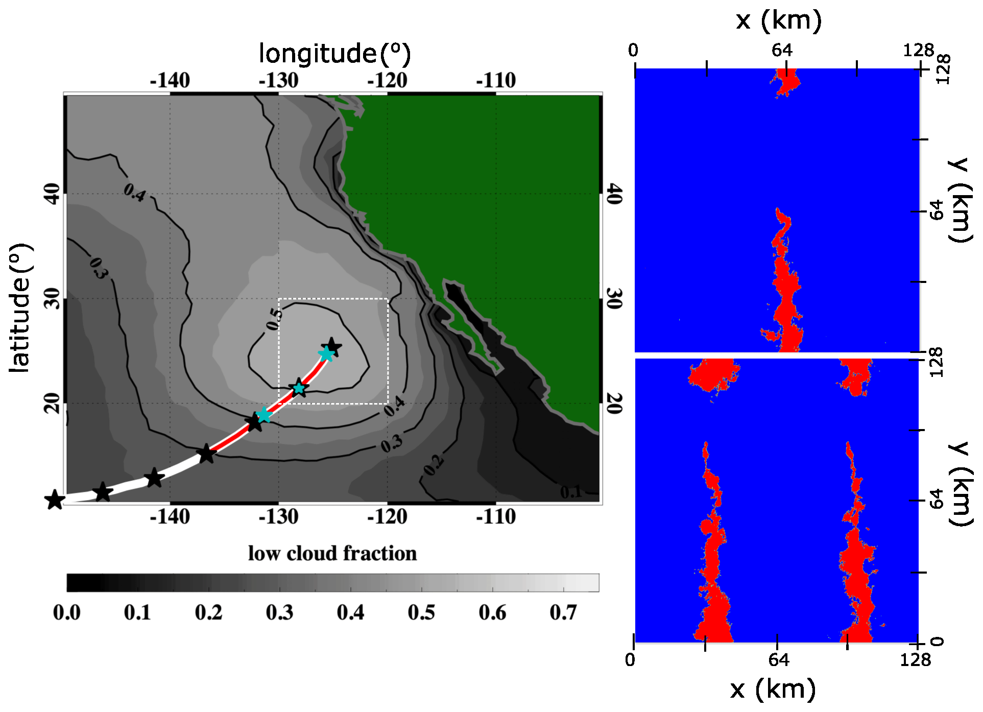
Figure 1The white curve is the 6 d Lagrangian trajectory identified by Sandu et al. (2010) in the NEP. The red curve is the 3 d Lagrangian trajectory simulated here (see Sandu and Stevens, 2011; Yamaguchi et al., 2017). The contours represent the marine low-cloud fraction obtained from Aqua-MODIS between 2005 and 2014. The dashed white square box indicates the region studied by Klein and Hartmann (1993). The black stars indicate the air parcel position at 24 h intervals, and the cyan stars are the positions of each aerosol pulse. Each aerosol pulse may have one or two active sprayers. The panels to the right represent the one- and two-sprayer configurations. The red (blue) areas in these two panels represent the plume track (background) in the NA150 case identified using the methodology described in the Appendix.
We use the System for Atmospheric (SAM) model as the LES dynamical core (Khairoutdinov and Randall, 2003). The radiative effects are represented using the Rapid Radiative Transfer Model for Global Climate Models (RRTMG) with extended vertical profiles above the domain top (Mlawer et al., 1997). The microphysical scheme consists of two modes representing cloud droplets and raindrops separately, allowing for more precise bin-by-bin mass transfer rates for modeling the collision–coalescence processes (bin-emulating). The size distributions are represented as log-normal distributions, each with a fixed geometric standard deviation of 1.2 (Feingold et al., 1998; Wang and Feingold, 2009a). The two modes are separated by a threshold value of 25 µm in radius (Kessler, 1969; Khairoutdinov and Kogan, 2000). Additionally, a separate prognostic equation is solved for Na, which includes a fixed surface flux of 70 cm−2 s−1 (Kazil et al., 2011), and losses or gains through cloud processing (activation, deactivation, collision–coalescence, and wet removal). The activation of aerosol particles is determined by the local supersaturation, which is calculated prognostically following the semi-analytical method of Clark (1973). The aerosol follows a log-normal size distribution with a geometric standard deviation of 1.5 and a geometric mean radius of 100 nm (Yamaguchi et al., 2017). In the applied modeling framework, cloud processing of aerosol affects the number concentration of aerosol but not the shape of the distribution (Feingold et al., 1998; Yamaguchi et al., 2017). Note that the recommended radius of aerosol particles for MCB is thought to be between 15 and 85 nm (Wood, 2021; Haywood et al., 2023), which is slightly smaller than the size range considered. We assume the injected particle size distribution to be the same as the background size distribution to avoid treating two separate populations, which would in any case become indistinguishable once processed by the cloud. This differs from the more rigorous aerosol treatment using the superdroplet approach (Hoffmann and Feingold, 2021; Prabhakaran et al., 2023; Hoffmann and Feingold, 2023), which is computationally unfeasible for the long simulations and large domains used here. In spite of this simpler aerosol and cloud microphysical treatment, the results are highly relevant in terms of the injection-related modification to Nd and the subsequent adjustments of LWP and fc, which together determine the degree of cloud brightening.
All the simulations have a domain size of 128 km in the horizontal directions and 4.25 km in the vertical direction. A uniform grid spacing of 100 m is used in the horizontal directions. In the vertical direction, a uniform grid spacing of 10 m is used below 2.775 km, and above this height, the grid is smoothly stretched to the domain top with the grid spacing increasing linearly with height. The total number of grid points in the vertical direction is 300. Such a large horizontal domain is chosen to capture the spread rates of the injected aerosol plume, as well as precipitation and associated cloud-field organization (Wang and Feingold, 2009b; Yamaguchi et al., 2017). The time step is set to 3 s with adaptive sub-stepping to satisfy the Courant–Friedrichs–Lewy stability condition. The radiative heating profiles are updated every minute. The simulation is integrated in time for 3 d, starting on the 196.75th day of the year (15 July 10:00 local time).
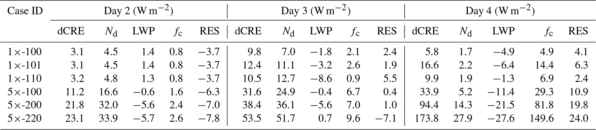
Table 1Cloud radiative effect enhancement (dCRE = CRE0×-000 − CREcase ID) and its decomposition at the TOA for all the seeded cases in NA150. The budgeting is done using cloud properties for a threshold of τ > 2. The quantity for each day is averaged between sunrise and sunset. On day 4, the averaging is done between sunrise and simulation end time. Column RES is the residual of the dCRE budget. RES = dCRE − sum of dCRE components.
Two sets of simulations are conducted for different baseline Na: 150 mg−1 (NA150) and 50 mg−1 (NA50). In the baseline case in NA150, the transition from overcast stratocumulus to low-cloud-fraction (fc) clouds occurs due to the increasing SST. The timescale of the transition is determined by precipitation. On the other hand, in the NA50 baseline case, the transition is solely driven by precipitation resulting in an open-cellular cloud structure. Note that the precipitation-driven transitions are reversible (i.e., overcast stratocumulus layer can be re-established) if a sufficient amount of aerosol particles is injected into the boundary layer (Feingold et al., 2015). In our study, the transition is said to be complete when fc decreases to a value below 40 % and stays below this value for at least 6 h. Both NA150 and NA50 systems are subjected to various aerosol seeding strategies summarized in Tables 1 and 2. We vary aerosol injection rates: low (1×10¹⁶ particles s−1 referred to as 1×) and high (5×10¹⁶ or 8.6×10¹⁶ s−1 referred to as 5× and 8.6×, respectively), which are the recommended ranges per sprayer for MCB (Wood, 2021). Note that the 8.6× injection is explored only for the NA50 system. We also vary the number of aerosol sprayers and the number of aerosol pulses along the trajectory. A schematic of the trajectory, the position of the aerosol pulses, and the configuration of the sprayers is provided in Fig. 1. Each seeding strategy has a five-character code (e.g., 1×-120). The two characters before the hyphen represent the strength of the aerosol injection rate (0×/1×/5×/8.6×), and the last three digits represent the number of sprayers (0/1/2) active during each of the three aerosol pulses. A value of 0 indicates that no aerosol is injected during the time period of that pulse. The first aerosol pulse is introduced 4 h after the start of the simulation. The next pulse is introduced approximately 20 h after the first pulse, and the final pulse is introduced 19 h later. An approximately 20 h separation between pulses is maintained to ensure sufficient time for the aerosol plume to spread across the domain. During this time the cloud layer advects approximately 350 to 400 km. The total aerosol injected into the marine boundary layer can be calculated as the aerosol injection strength times the sum of the last three digits in the code. Each aerosol pulse represents the passage of sprayer(s) upstream from one end of the domain to the other at a speed of 5 m s−1; i.e., the relative speed between the sprayer and the domain is 5 m s−1. Each sprayer has the dimension of one grid cell (100 × 100 m2), and all the particles are injected from the surface.
3.1 NA150: polluted system
Figure 2a shows the time evolution of the injected aerosol plume areal coverage. The injected plume is distinguished from the background by setting a threshold on the vertically integrated boundary layer aerosol concentration (). A plume is identified when exceeds the background variability in Na (see Appendix A for more details). Ideally, for MCB applications one should consider cloud optical thickness (τ) or cloud albedo (Acld) for identifying the plume. However, the signal from these quantities is not very strong for the polluted system, especially in the 1× cases. To leading order, the plume coverage increases linearly with time in all cases (Fig. 2a). The spread rate is approximately 2 times faster for the two-sprayer configuration compared to the single-sprayer configuration, which is expected. The spread rates are qualitatively similar for the 1× and 5× cases, although the 5× cases appear to be spreading at a faster rate. Note that the turbulent kinetic energy (Fig. 3), which is a measure of mixing within the MBL, is similar in all the cases, until the onset of precipitation, which occurs in the morning of day 3 (≈ 35 h after the start of injection). Thus, for a given number of sprayers, the plume spread rates are for the most part not affected by the number of aerosol particles injected. Therefore, the slower spread rate in the 1× cases is an artifact of the plume detection methodology. In the 1× cases, along the plume edges, the absolute value of Na becomes comparable to the background value (low signal-to-noise ratio) after some time due to dilution. This reduces the detected plume area, as is evident from the decrease in plume area coverage in the 1× cases after sunset on day 2.
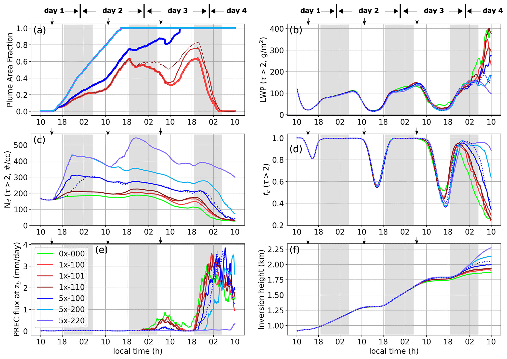
Figure 2Time series of (a) plume area coverage, (b) liquid water path (LWP), (c) cloud droplet concentration (Nd), (d) cloud fraction (fc), (e) domain-averaged precipitation flux (rain rate) at cloud base zb, and (f) domain-averaged height of the inversion layer (zi) in NA150. τ is the cloud optical thickness. The legend is shown in panel (e). The dotted lines in panels (b)–(f) are the cloud properties in case 5×-100 with a delayed aerosol perturbation. The perturbation is delayed by 5 h (relative to 5×-100). The downward-pointing arrows at the top of each panel represent the time at which the three aerosol pulses start spraying, if active. Note that all the time series plots in this article start at 10:00 LT on day 1 and end at 10:00 LT on day 4.
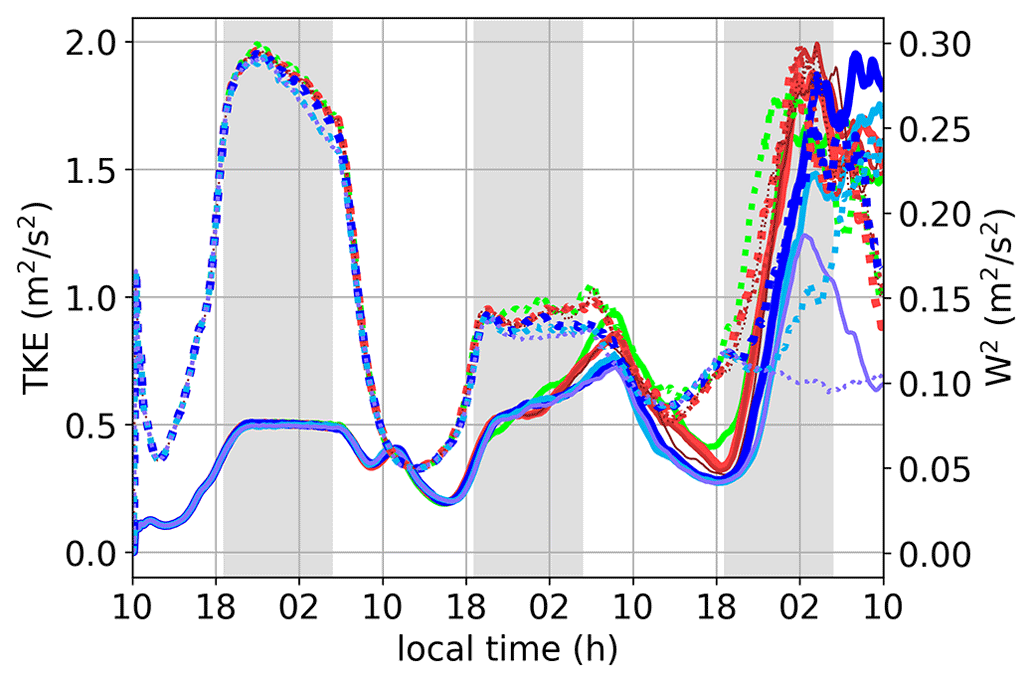
Figure 3Time series of the resolved turbulent kinetic energy (TKE) (solid lines) and resolved vertical velocity variance (w2) (dashed lines) at 700 m in NA150. See Fig. 2e for the color code.
Regarding the plume area fraction, a value of unity is an outcome of the limited horizontal domain. This restricts the scope of this study in the context of ship tracks because “real” tracks evolve in an “infinite” domain and never reach an area fraction of 1. Consequently, the cloud properties would be continuously affected by spreading and dilution of the track. However, in the context of MCB, the primary focus here, several sprayers are operating in tandem. An area fraction of unity indicates that multiple plume tracks have merged, and no more dilution due to spreading is occurring.
Figure 2b, c, and d depict the evolution of the cloud-averaged properties conditional on τ>2: liquid water path (LWP ∣ τ>2), cloud droplet concentration (Nd ∣ τ>2), and cloud fraction (fc ∣ τ>2), respectively. Note that we have not separated the plume and background regions when calculating these properties. In the baseline case (0×-000), barring the variability associated with the diurnal cycle, the LWP increases with time in response to the increasing SST and associated MBL deepening (Fig. 2f). This trend continues until day 3 in the afternoon. Nd is nearly constant for the first 2 d. The reduction in Nd due to weak collision–coalescence is offset by the steady flux of aerosol from the ocean surface. In the morning hours of day 3, the LWP is high enough to cause precipitation at cloud base (zb) on the order of 0.5 mm d−1 (Fig. 2e). On day 3, Nd decreases by about 40 % by midday due to (i) collision–coalescence and precipitation losses and (ii) a likely reduced aerosol activation rate due to the weakening of the updrafts (Fig. 3) from precipitation evaporation and SW absorption. The subsequent recovery in LWP late in the afternoon triggers runaway precipitation that removes aerosol from the MBL and breaks up the stratocumulus layer. This is evident from the time series of fc, which follows the familiar diurnal cycle up to day 3 in the morning. The weak (< 1 mm d−1 at zb) precipitation in the morning and the afternoon enhances the daytime reduction in fc slightly. However, post-sunset, the cloud system recovers and generates sustained stronger precipitation (on the order of 3 mm d−1 at zb), eventually reducing fc to below 30 % by the end of the simulation.
Nd increases in all the perturbed cases. After the initial linear increase, while the sprayer is active, in the weakly perturbed cases (1×), Nd is nearly constant in time until the morning of day 3. This is similar to the baseline case. In the strongly perturbed cases (5×), there is a steady decrease in Nd with time consistent with the deepening of the MBL (Fig. 2f). The 1× and baseline cases are not affected by this deepening because the difference in Na between the free troposphere (150 mg−1) and the MBL (150–200 mg−1) is not significant, unlike in the 5× cases. Note that in realistic conditions, a strong gradient in Na can exist between the free troposphere and the MBL. Under those conditions, MBL deepening should be considered an added factor influencing the evolution of Nd (Yamaguchi et al., 2015). In the LWP time series (Fig. 2b), no significant changes are evident on day 1 in the perturbed cases as the plume coverage is quite small (Fig. 2a). A weak negative LWP adjustment is visible around midnight on day 2, where the baseline case has the highest LWP, and the value in the perturbed cases is lower depending on the total aerosol particles injected into the MBL. The negative LWP adjustment here is an outcome of the entrainment feedback associated with the reduction in the sedimentation flux of droplets (Bretherton et al., 2007) and enhanced evaporation rate near the cloud top (Wang et al., 2003). During this time, fc in all the cases is identical. Note that the entrainment velocity (we) is inferred from changes in the inversion height (, where D is the large-scale divergence of the horizontal velocity field).
At sunrise on day 3, in the seeded cases, injection of aerosol suppresses precipitation and increases LWP relative to the baseline case (Fig. 2b, e). The degree of precipitation suppression is proportional to the amount of injected aerosol to that point in time. However, the gain in LWP is not directly proportional to the degree of precipitation suppression but is partly offset by entrainment effects (Fig. 2f). Furthermore, the increased Nd sustains slightly higher LWP relative to the baseline case until midday, after which the LWP in the seeded cases decreases below that of the baseline case. Similarly, higher Nd also sustains higher fc in the morning and lower fc in the afternoon. This reduction in LWP and fc is due to enhanced SW absorption associated with the higher LWP and Nd in the morning (Fig. 4). The subsequent recovery in LWP and fc late in the afternoon and early evening triggers strong precipitation in all the cases and significantly depletes Na and Nd within the MBL. The precipitation (≈ a few mm d−1) breaks up the stratocumulus layer, as is evident from the decreasing values of fc. The onset of the break-up (or transition) is controlled by the amount of aerosol injected into the MBL. The delay in the onset of the break-up is proportional to the number of injected particles into the MBL and is delayed the most in case 5×-220 (Fig. 2e). By the end of the simulation (morning of day 4), weak precipitation has started in case 5×-220. A longer simulation would be required to determine whether this would lead to the break-up of the stratocumulus layer. Additionally, suppression of precipitation deepens the boundary layer, as is evident from the inversion height (zi) on days 3 and 4 (Fig. 2f).
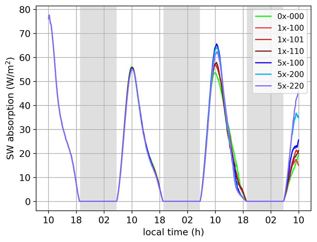
Figure 4Time series of the SW absorption by the cloud layer in NA150. See Fig. 2e for the color code.
Figure 5a shows the Lagrangian evolution of the vertical profiles of Na+Nd in case 5×-100, with the cloud-top and cloud-base heights marked by black lines. Figure 5b shows snapshots of Na+Nd at intervals of 8 h. Figure 5c shows the vertical integral of sub-cloud negative buoyancy flux integral, BFI = (∀ z<zb; ), a measure of the decoupling between the cloud layer and surface (Bretherton and Wyant, 1997; Prabhakaran et al., 2023). The minimum criterion for decoupling is BFI < 0 because vertical turbulent kinetic energy (TKE) is destructed, thus limiting vertical mixing. Here, and w′ are fluctuating components of virtual potential temperature and vertical velocity, respectively, and the overline represents the horizontal average. The vertical profiles indicate that the boundary layer is well-mixed until sunrise on day 2, which is supported by the near-zero BFI. Thus, the injected aerosol from the first aerosol pulse mixes throughout the layer. On day 2, the boundary layer is deeper, but the vertical mixing is weaker due to the enhanced SW absorption from the increase in LWP. This is reflected in the increase in the (negative) magnitude of BFI. The same is evident from the accumulation of aerosol emitted from the ocean surface in the lower levels of the MBL. Post-sunset on day 2, the cloud layer continues to deepen, which further strengthens the decoupling from the surface. This continued deepening triggers weak collision–coalescence and precipitation on the morning of day 3, accompanied by diverging values of BFI (around 02:00 LT). Note that runaway precipitation only occurs after the recovery of LWP and fc during the night on day 3.
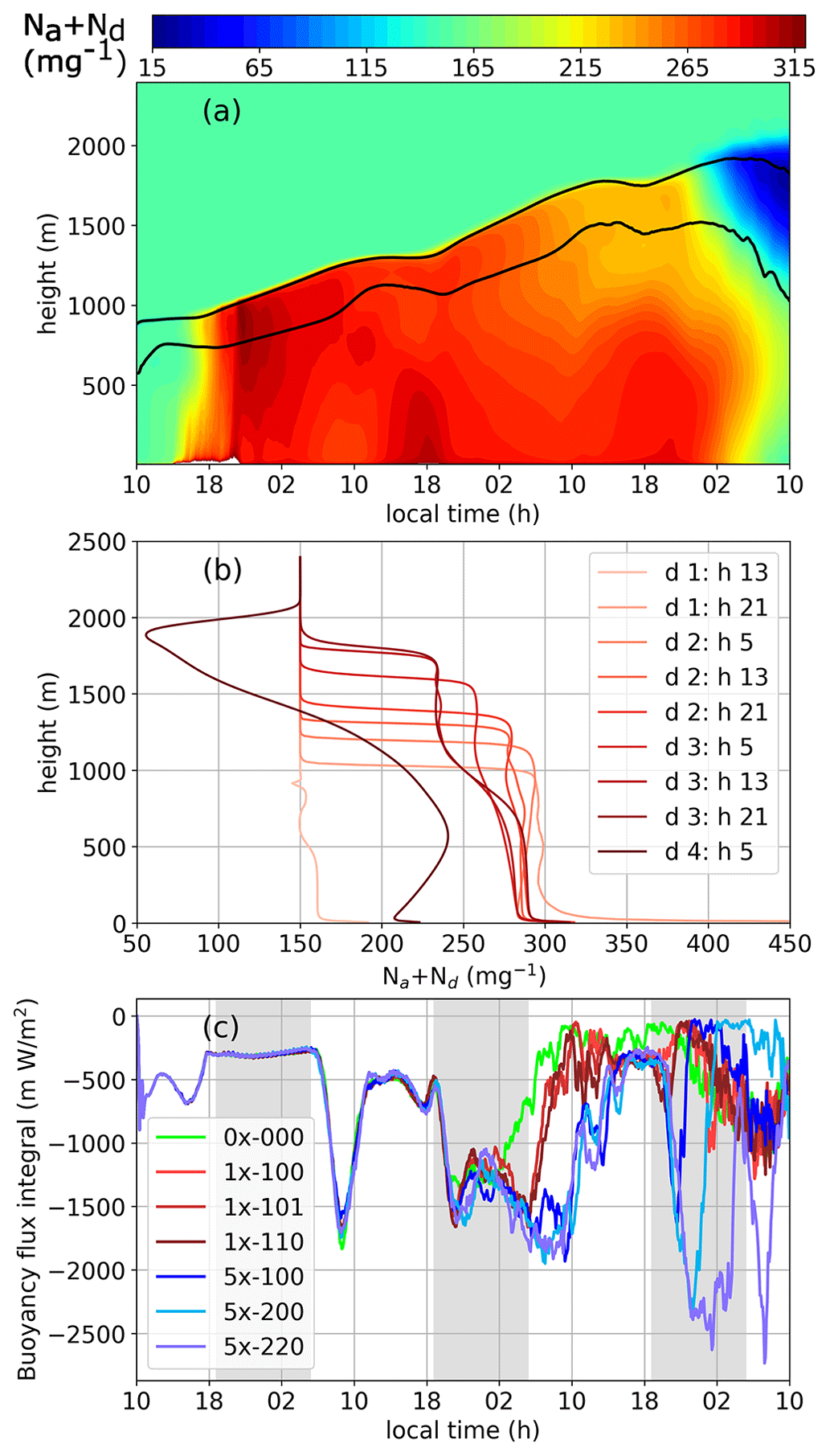
Figure 5(a) Lagrangian curtains of Na+Nd in case 5×-100, with the black lines representing cloud base and cloud top. (b) Vertical profiles of Na+Nd at select times (“d” is the day and “h” is the hour of the day). (c) Sub-cloud negative buoyancy flux integral, a measure of the degree of MBL mixing for all the cases. At any instant, more negative values of BFI indicate poorer vertical mixing.
The onset of weak precipitation increases mixing within the sub-cloud layer, as indicated by the BFI approaching zero in the 1× cases between 02:00 and 12:00 LT on day 3. The strong suppression of precipitation in the 5× cases enhances the decoupling due to increased cloud-top entrainment and MBL deepening (see the values of BFI between 02:00 and 10:00 LT on day 3). For 5×-100, this enhanced decoupling associated with precipitation suppression is also evident from the vertical profiles of Na+Nd in Fig. 5b (e.g., d 2, h 5). This decoupling is sustained until the onset of runaway precipitation (e.g., d 2, h 13 and d 2, h 21 in Fig. 5b).
Cloud radiative effect
To assess the impact of the various seeding scenarios under polluted conditions, we explore the changes to the cloud radiative effect CRE = , where Fin is the incoming solar radiation. Figure 6a shows the changes to the CRE (dCRE = CRE0×-000 − CREcase ID) at the top of the atmosphere (TOA) relative to the baseline in all the seeded cases. No significant changes to CRE are detected on day 1 as the injected aerosol plume track is quite narrow. By day 2, we see a substantial enhancement in the CRE in all the seeded cases. On day 3, the dCRE continues to grow. In some cases, this is due to an increase in aerosol concentration, but even in cases like 1×-100 and 5×-200 where no additional aerosol is added compared to day 2, we see a greater enhancement in dCRE on day 3. Note that the bulk of the dCRE enhancement occurs in the morning with a dominant peak around 08:00 to 10:00 LT. A similar result is evident in the simulations of Prabhakaran et al. (2023). In the absence of precipitation, the clouds are thicker in the morning with near 100 % cloud coverage. The absorption of incoming SW radiation reduces the LWP and fc in the afternoon. Consequently, the enhancement in CRE is greatest in the morning. In the afternoon of day 3, there is a hint of cloud darkening. The reason for this is discussed below, along with the dCRE decomposition. On day 4, there is a strong spread in dCRE due to variation in the timing of the transition. In the 1× cases, the dCRE is negligible, whereas the 5× cases with two sprayers show a substantial increase in dCRE. In particular, 5×-220 shows the highest enhancement, with a morning peak value of about 250 W m−2, which is well above the peaks on days 2 and 3.
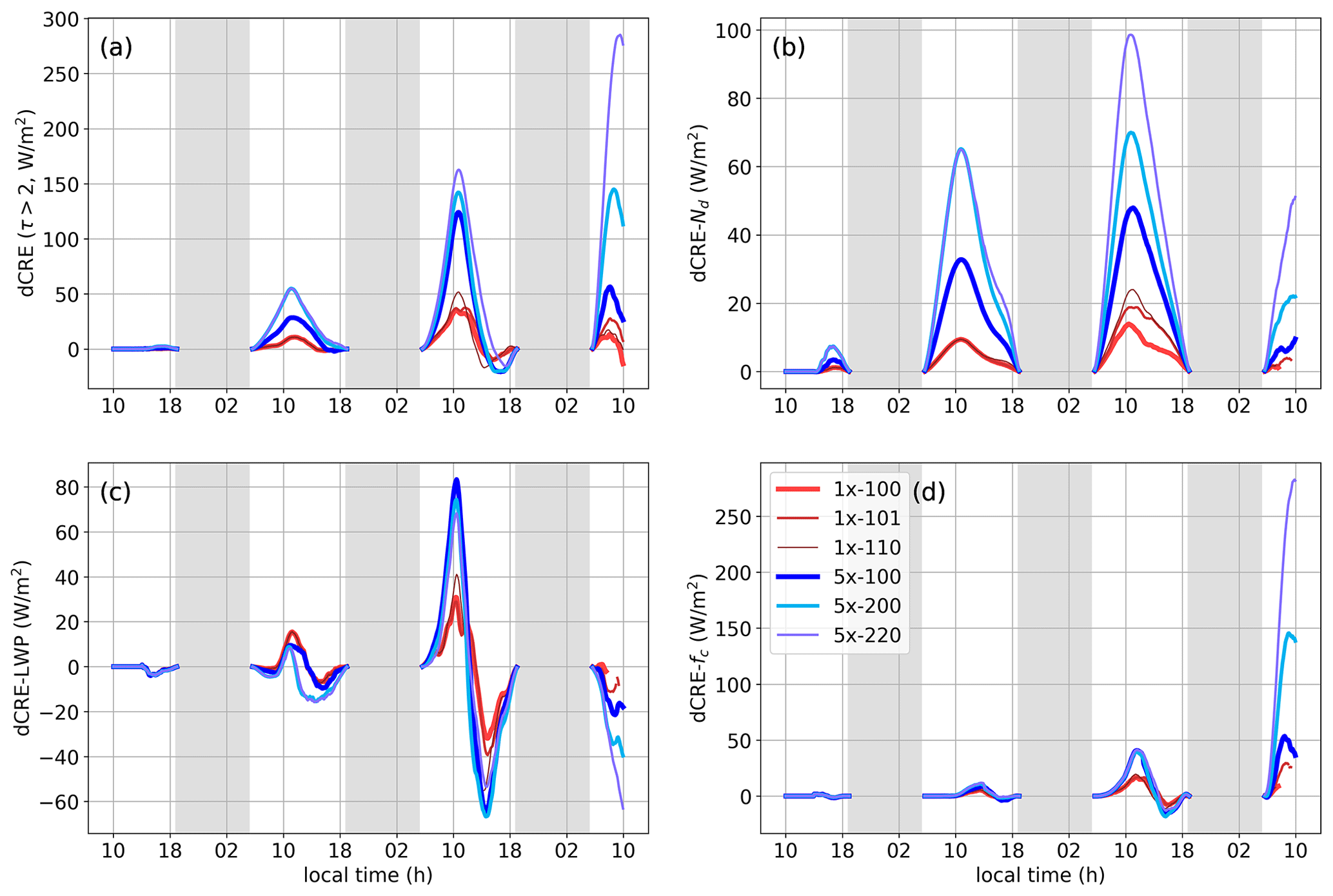
Figure 6Time series of changes in CRE relative to the unseeded case and its contributions. (a) dCRE, (b) Nd contribution to dCRE, (c) LWP contribution to dCRE, and (d) fc contribution to dCRE. τ is the cloud optical thickness. The legend is shown in panel (d).
In order to obtain further process level insights, we decompose dCRE to three contributions: Nd (dCRE), LWP (dCRELWP), and fc (dCRE). We follow the procedure laid out in Diamond et al. (2020) and Chun et al. (2023). The dCRE decomposition is written as
where Aclr is the clear-sky albedo; is the cloud albedo contribution from Nd or alternatively LWP; f is cloud fraction; AFpl is plume fraction; and the 0×, pl, and bg subscripts indicate the baseline case, in-plume track, and off track (background), respectively. Note that dCRE has contributions from both fc and Acld adjustments, which is an outcome of the multiplicative nature of the contributions from Acld and fc to CRE (∝ fc Acld). For instance, strong changes in fc are typically associated with precipitation. Under these conditions, LWP and Nd, and consequently Acld, are not constant. Therefore, dCRE has contributions from Acld that are not captured in the other two components (dCRE and dCRELWP). The residual from this budget is calculated as RES = dCRE − dCRE − dCRELWP − dCRE. Note that the budget model (Eq. 1) is based on mean-field properties, and does not account for the presence of inhomogeneities within the domain. Thus, the residual is a measure of the accuracy of the dCRE budget and of the inhomogeneities within the domain (Feingold et al., 2022).
Figure 6b–d show the time series of individual contributions to dCRE from Nd, LWP, and fc, respectively. Table 1 provides averaged values between sunrise and sunset for each day. Below, percentage contributions of the three components to dCRE are calculated as 100 × dCRE dCRE using the data from Table 1. The dCRE component is positive and substantial on days 2 (over 100 %) and 3 (70 %–100 %). In the cases where no additional aerosol is injected after the first pulse, the dCRE component increases from day 2 to day 3 in the single-sprayer configuration (e.g., 5×-100 or 1×-100), whereas in the twin-sprayer configuration (e.g., 5×-200), the contributions are similar in magnitude, with a slightly higher contribution on day 3 because of the suppression of precipitation in the morning. In the single-sprayer configuration, apart from the effect of precipitation suppression, the greater areal coverage of the plume on day 3 results in a higher dCRE component. On day 4, the dCRE is less than 20 % of dCRE. The dCRELWP component is much lower than that of dCRE on day 2, but the two are comparable in magnitude on day 3. Additionally, the LWP contribution is positive in the morning and negative in the afternoon. On day 3, the positive contribution is an outcome of precipitation suppression in the morning. Some of these positive contributions are offset by the effects of entrainment, which explains the lack of a consistent trend in the 5× cases. For instance, case 5×-220 has the strongest precipitation suppression (Fig. 2e), but cases 5×-100 and 5×-200 exhibit higher LWP and dCRELWP in the morning. However, in the afternoon, the dCRELWP is negative, with the highest magnitude for cases 5×-100 and 5×-200, due to the negative LWP adjustment from enhanced SW absorption. The higher LWP in these cases in the morning makes them susceptible to SW absorption, as is evident from the weakly negative dCRE in the afternoon. A similar conclusion was obtained in an earlier study (Prabhakaran et al., 2023). On the morning of day 4, the LWP component is negative and comparable in magnitude to the Nd component. Both of their contributions to dCRE are low (< 20 %). On this day most of the contribution to dCRE is from the changes in fc due to precipitation suppression.
From day 2 to day 4, the decoupling of the cloud layer from the surface increases, which favors the development of cumulus clouds. Moreover, the onset of precipitation further reduces the homogeneity within the domain. All of these contribute towards an increase in the magnitude of residual from day 2 to day 4 (column RES in Table 1).
3.2 NA50: pristine system
Figure 7, analogous to Fig. 2, shows the evolution of cloud and aerosol properties in the system with Na = 50 mg−1. The lower initial Na leads to an early onset of precipitation, even before the introduction of the first aerosol pulse (Fig. 7e), which leads to a very different aerosol plume and MBL evolution. In the baseline case, the precipitation-induced transition results in an open-cellular cloud structure. This structure is maintained until the end of the simulation. Note that the boundary layer is quite shallow, which supports the open cellular structure (Fig. 7f). This makes the transition reversible through aerosol addition (Feingold et al., 2015).
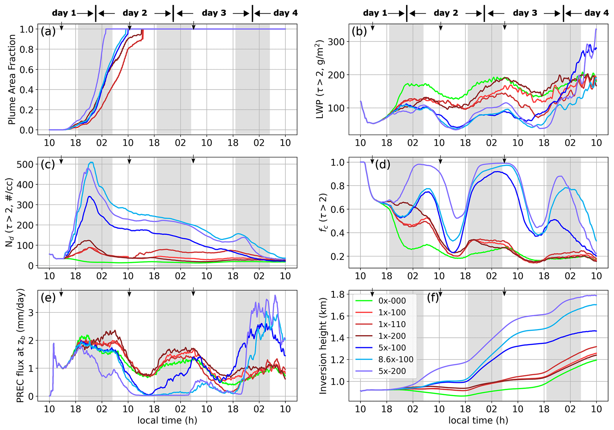
Figure 7a shows the evolution of plume area coverage. Qualitatively, its evolution is similar to the NA150 system with a monotonic increase in time. However, the spread rate in the current system is higher. For instance, case 5×-200 in NA150 attained a plume area fraction of 0.9 on day 2 around 12:00 LT. The same case in NA50 attains a similar plume area fraction on day 2 by 03:00 LT. A higher spread rate in NA50 is related to the flow patterns in the precipitating and precipitation-suppressed regions, which is discussed further in Sect. 3.2.1 below.
Figure 7b, c, and d show the cloud properties LWP, Nd, and fc, respectively. In the baseline case, Nd and fc decrease after the onset of precipitation. The (cloudy-average) LWP shows an increasing trend, as expected in broken cumulus. The stronger updrafts associated with the convergence of surface flows form deeper clouds with higher LWP, although at the cost of low fc (Wang and Feingold, 2009a).
In all the perturbed cases, the impact of the seeding is visible in the Nd time series immediately and in the LWP and fc time series after about 20:00 LT on day 1. Injection of aerosol increases Nd and fc and lowers the LWP relative to the baseline case for much of the duration of the simulation. These reductions in LWP are attributed to the deepening of the MBL (Fig. 7f) and manifest more strongly because of the reduction in fc. After the initial increases in Nd while the sprayers are active, there is a strong decline (especially in the strong perturbation cases). This decline continues until the aerosol plume spreads across the domain (approximately the middle of day 2). This reduction is due to the ongoing collision–coalescence along the plume track boundaries.
In the 1× cases, the rain rate is slightly lower than the baseline for a few hours post-injection (day 1, approximately 20:00 LT). This decrease in precipitation is proportional to the number of injected aerosol particles. During this time the local (plume track) cloud coverage approaches 100 %. By the end of day 1, precipitation in the 1× cases recovers and exceeds the baseline value, while fc decreases subsequently, albeit at a slower rate than the baseline case. The higher domain-mean precipitation rate relative to the baseline case is sustained by the generation of non-precipitating or weakly precipitating clouds with lower LWPs and higher Nd occurring over a larger fraction of the domain (higher fc). Over time, as the aerosol plume spreads, Nd decreases locally within the plume track (not shown in Fig. 7c). This lowers the colloidal stability of the clouds, resulting in precipitation and subsequent cloud break-up. By the afternoon of day 2, fc in the 1× cases is below 0.3 (comparable to the baseline case) with no signs of recovery.
For the higher seeded amounts, the injection of aerosol reduces precipitation significantly for the first 2–3 d (depending on the strength of the injection), allowing the boundary layer to establish a stratocumulus layer with fc close to 1. Unlike in the 1× cases, the number concentration in the aerosol pulse is high enough to suppress precipitation in adjacent cells due to lateral spreading. The suppression of precipitation allows the MBL to deepen, which decreases Nd as a result of dilution (Fig. 7f). Subsequent precipitation events towards the end of day 3/day 4 result in a runaway effect and cloud break-up, marking the transition to cumulus clouds.
The counteracting effects on Nd of aerosol injections and MBL deepening play out in an interesting manner in cases 5× and 8.6×. Wang et al. (2011) argued that a concentrated injection is more effective than a distributed injection in enhancing the CRE in the presence of strong precipitation. The 8.6×-100 case can be considered a more concentrated version of 5×-200. Compared to case 8.6×-100, 5×-200 has more aerosol injected into the MBL; however Nd in these two cases is comparable – in fact, Nd is slightly higher for case 8.6×-100. The difference comes from the depth of the MBL (Fig. 7f). The MBL height in 5×-200 is about 100–200 m greater than in 8.6×-100. To leading order, the increase in fc and zi is proportional to the total injected aerosol number. Furthermore, the changes in LHF and sensible heat flux (SHF) in response to aerosol perturbations are broadly consistent with the deepening of the MBL (Fig. 8). The increased entrainment of drier and warmer free-tropospheric (FT) air enhances LHF and reduces SHF.
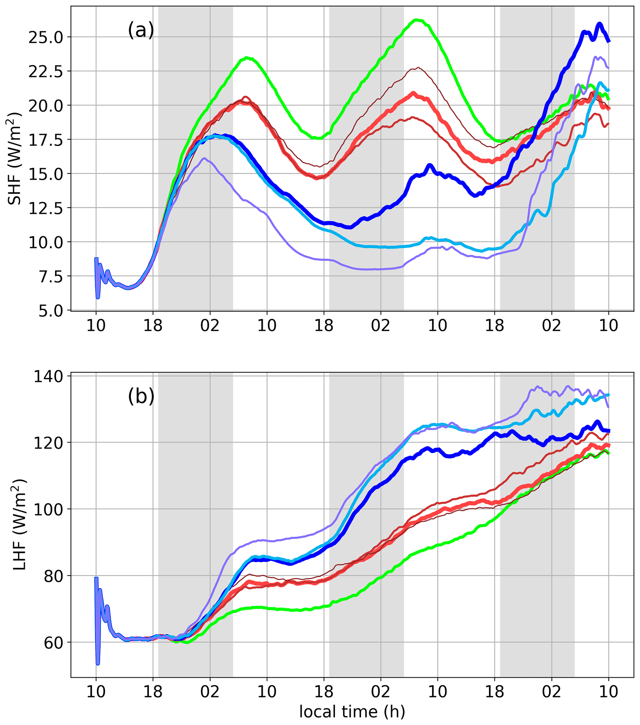
Figure 8Time series of surface scalar fluxes in all the cases in NA50. See Fig. 7 for legend. (a) Sensible heat flux (SHF) and (b) latent heat flux (LHF).
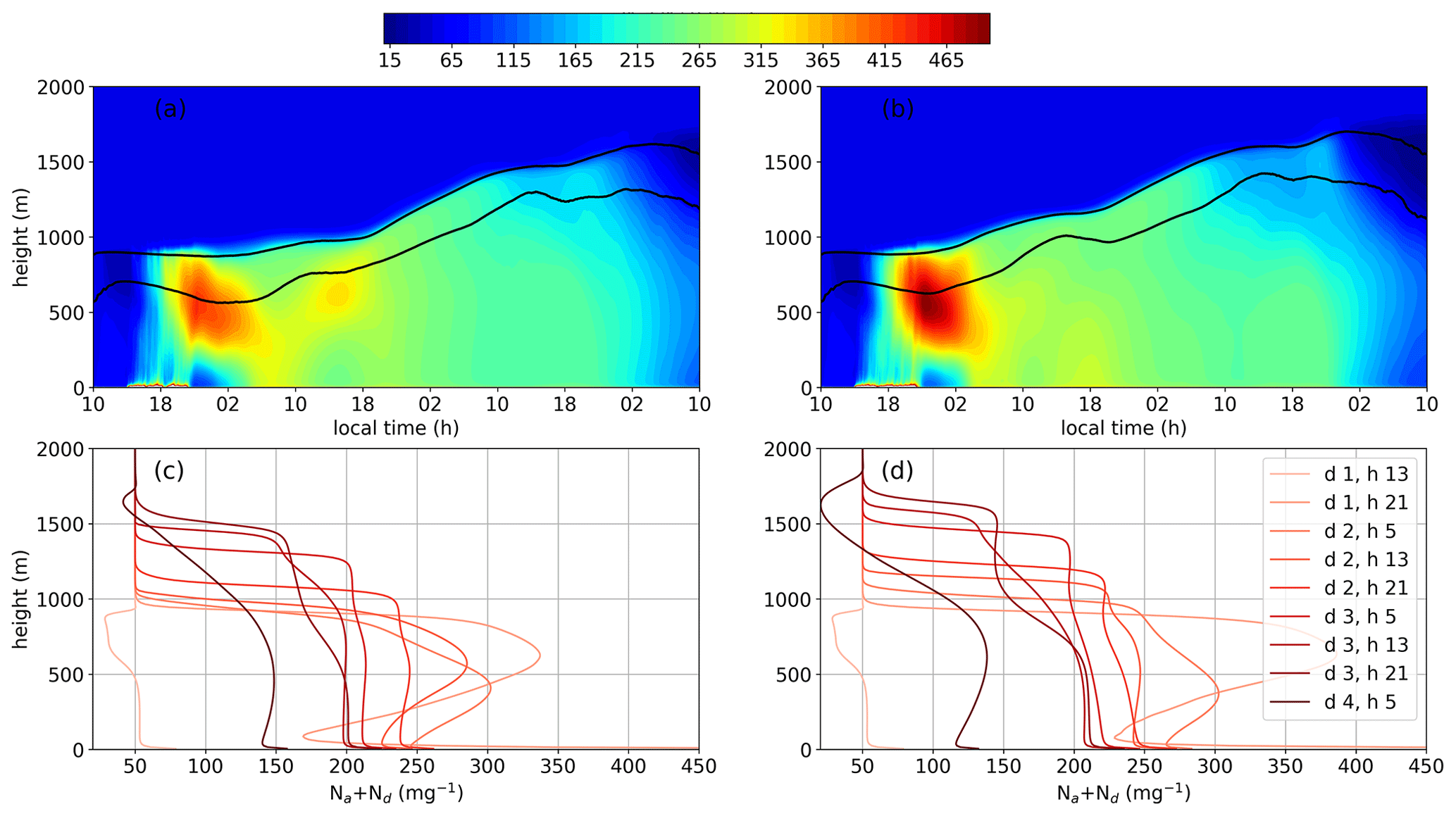
Figure 9NA50. (a, b) Lagrangian curtains of Na+Nd in cases 8.6×-100 and 5×-200, respectively. The black curves represent the cloud-base and cloud-top heights. (c, d) Vertical profiles of Na+Nd at intervals of 8 h in the cases shown in (a) and (b).
Figure 9a and b show the Lagrangian evolution of the vertical profiles of Na+Nd in cases 8.6×-100 and 5×-200. A few snapshots at intervals of 8 h are shown in Fig. 9c and d for further clarity. The earlier and stronger precipitation suppression in 5×-200 starts deepening the MBL by the morning of day 2, which strengthens the decoupling of the cloud layer from the surface. This is evident from the time series of the BFI (Fig. 10). Furthermore, the deepening of the MBL enhances the LHF and reduces the SHF (Fig. 8). The corresponding increase in LWP is higher in 5×-200 compared to 8.6×-100, which is evident in the afternoon of day 2 (Fig. 7b). Furthermore, the dilution associated with the deepening of the cloud layer and weaker net aerosol vertical transport from the surface layer maintains a lower Nd in 5×-200. Note that Na is higher in case 5×-200 close to the surface. Thus, the differences in the final cloud break-up time in these cases is a manifestation of the differences in the boundary layer structure post-aerosol injection.
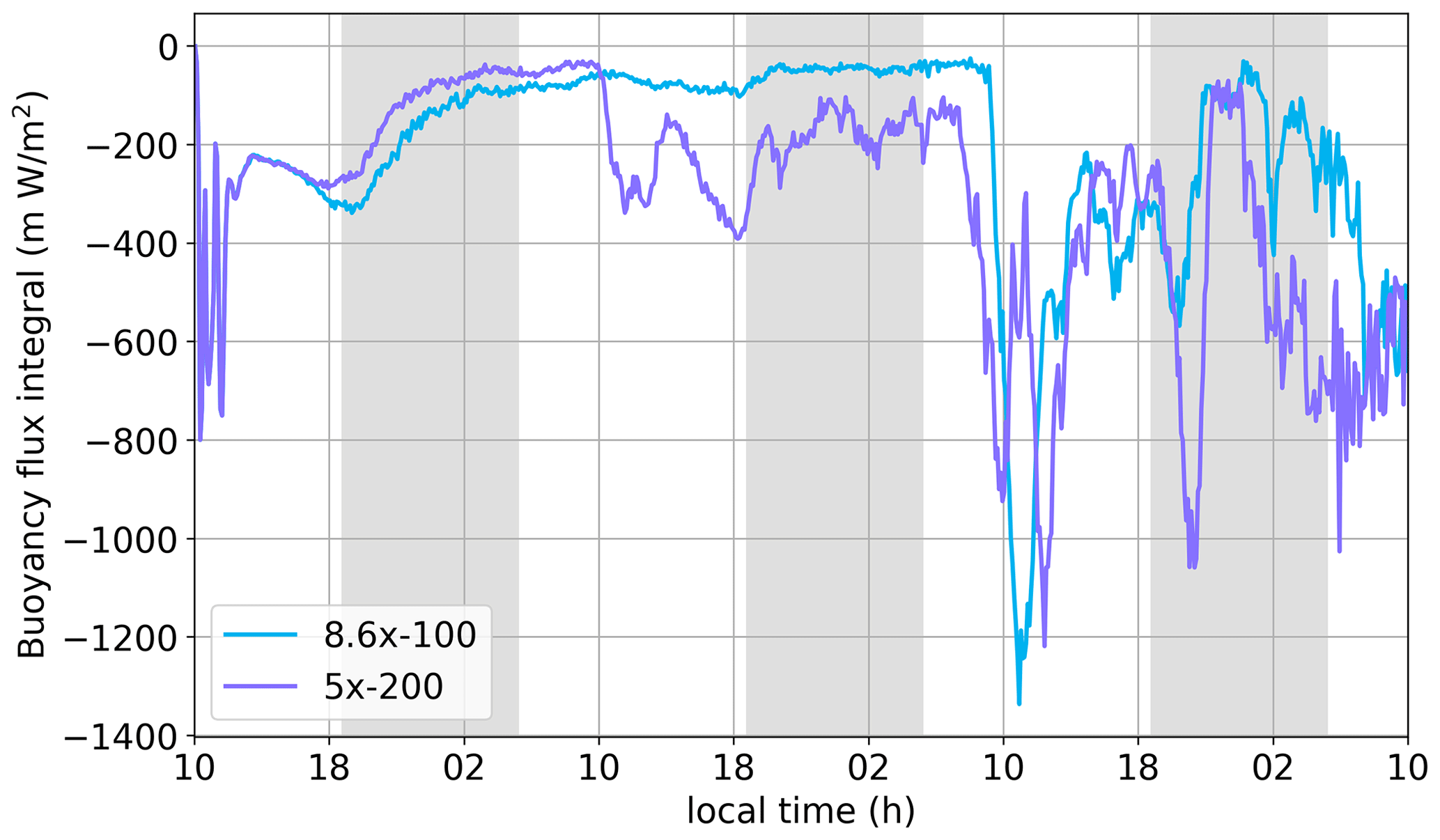
Figure 10Negative buoyancy flux integral in the sub-cloud layer in cases 8.6×-100 and 5×-200.
3.2.1 Transverse circulation
The faster dispersal of the injected aerosol plume in NA50 is associated with the formation of a transverse circulation across the aerosol plume track (Wang and Feingold, 2009b). The cross-sectional snapshots at different times in Fig. 11 show the flow patterns in the plume-affected region and its neighborhood for case 8.6×-100. Note that the vectors represent the velocity component after the mean horizontal wind has been removed. The x–y cross sections in Fig. 11a, c, and e show the organization of the flow-field from the circulation near the cloud top along the plume track and its brief evolution in time (about 9 h). This circulation is created by the presence of a gradient in the rain rate across the plume track, which causes a corresponding buoyancy gradient that directs the circulation (filled contours in Fig. 11b, d, and f). Initially, the plume track exhibits slightly positive buoyancy, which is contrasted by strongly negative buoyant regions outside the plume track associated with evaporating precipitation. The strong convergence near the surface along the track is associated with the outflows from the adjacent precipitating cells that supply moisture to the plume track, making it more positively buoyant (Fig. 11b, d). Hence, the injected aerosol particles are lofted to the cloud layer within strong updrafts with velocities around 1–3 m s−1 (Fig. 11b, d). This suppresses precipitation, which causes strong outflows near the cloud top at the top of the plume track. These outflows spread horizontally until they encounter a counter flow from a neighboring cloud cell (x ≈ 60 km in Fig. 11d). This deflects the polluted outflow towards the cloud base in the neighboring cell (Fig. 11d, f), aiding in the faster dispersal of aerosol. Note that the spread rate of the plume is affected by the strength of the perturbation, with the 5× cases having a faster spread rate compared to the 1× cases. This is an outcome of the difference in the strength of the transverse circulations. The positive feedback associated with stronger in-track precipitation suppression and subsequent moisture convergence results in a stronger circulation. A detailed discussion about this precipitation gradient-induced mesoscale circulation is provided in Wang and Feingold (2009b, Fig. 9b therein). Note that the meteorology and large-scale forcing in the current simulation are very different from those in Wang and Feingold (2009b), which supports the generality of this mechanism in the presence of aerosol gradients in a precipitating shallow boundary layer.
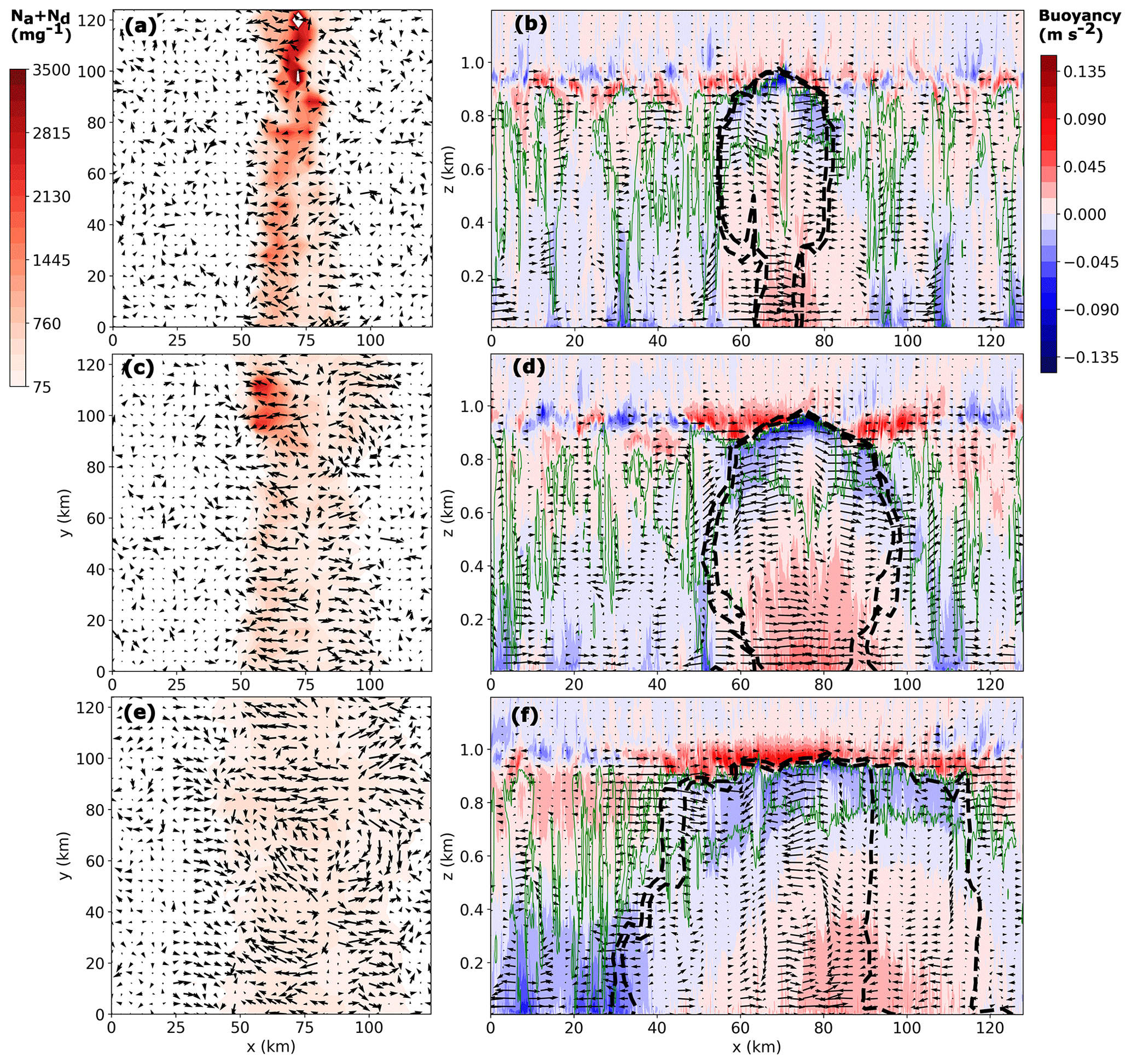
Figure 11(a, c, e) x–y cross sections of Na+Nd and (b, d, f) x–z cross sections of buoyancy, for the case 8.6×-100. The vectors represent the planar velocity field after subtracting the horizontal mean wind. x–y cross sections are at z = 700 m, and x–z cross sections are at y = 64 km. The green contour lines in the panels to the right indicate liquid water content of value 0.01 g kg−1, and black contour lines (dashed) represent values of Na+Nd = 100 and 200 mg−1. (a, b) t = day 0, 22:00 LT; (c, d) t = day 1, 01:00 LT; (e, f) t = day 1, 07:00 LT.
3.2.2 Cloud radiative effect
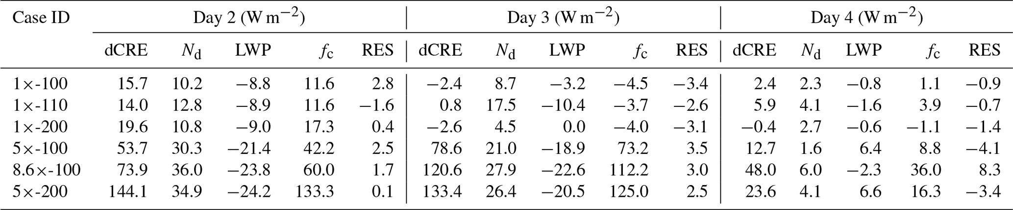
Figure 12a shows the time series of dCRE for the NA50 cases. In all the cases, we see a dominant peak in the morning around 10:00 LT, similar to the dCRE profiles in NA150. In the 1× cases, an enhancement in CRE is evident only on the morning of day 2. In the 5× and 8.6× cases, a substantial enhancement in CRE is evident on days 2 and 3. On day 4, the enhancement in CRE is significant but substantially weaker in comparison to the earlier days. This is due to the precipitation-related decrease in fc. Table 2 and Fig. 7b, c, and d show the contributions to dCRE from Nd, LWP, and fc, respectively. Note that the y-axis range is different for each panel. As in case N150, the percentage contributions of the three components to dCRE can be calculated from Table 2 as 100 × dCRE dCRE. The dominant contribution to CRE derives from the changes to fc in the strong perturbation cases. The contribution from Nd is positive, and its magnitude is less than 20 %–30 % of dCRE. In contrast, the contribution from LWP is negative and is comparable in magnitude to that of dCRE on days 2 and 3. Similarly, in the 1× cases, the Nd and LWP components are comparable in magnitude but of opposite sign.
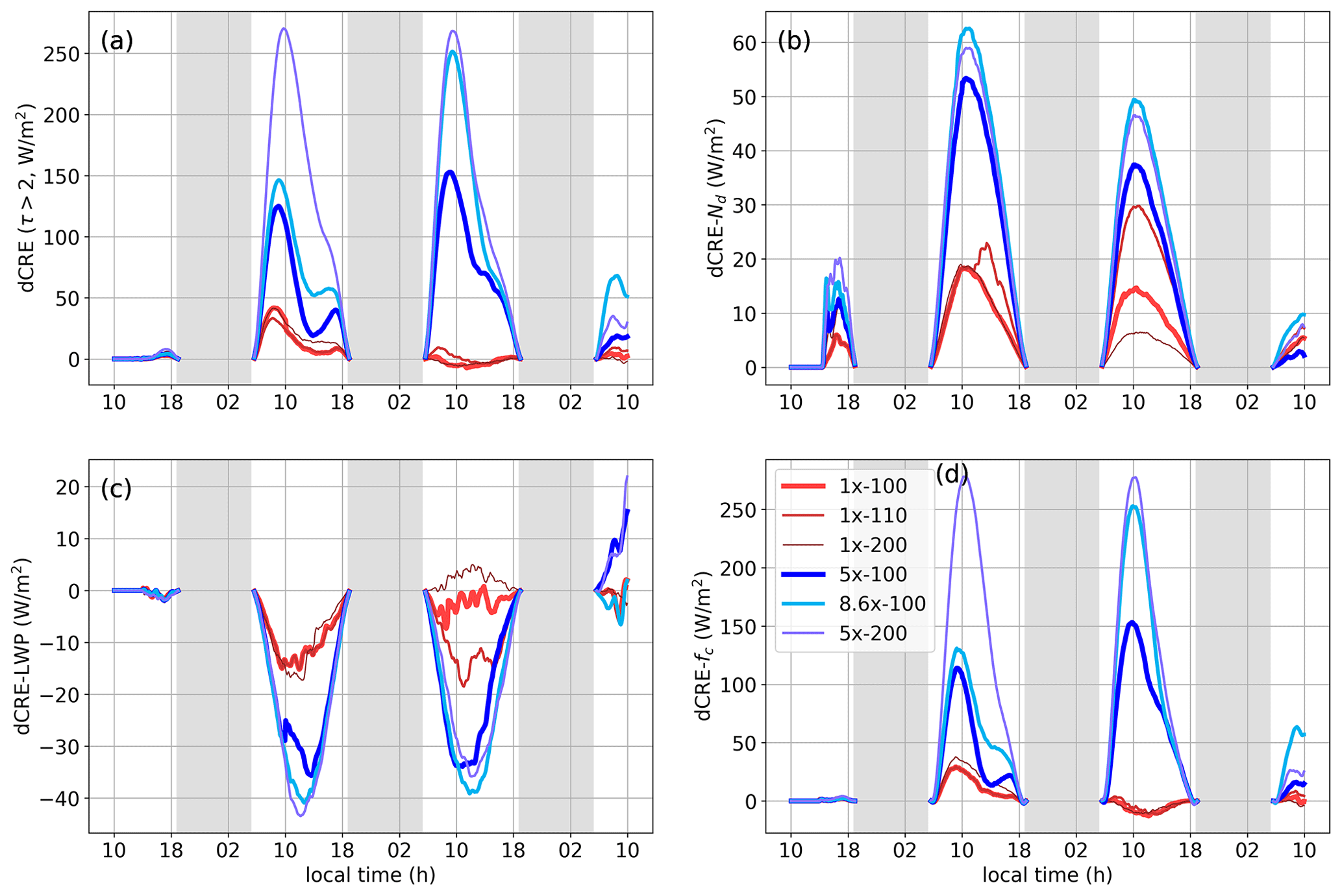
Figure 12Time series of changes to CRE (dCRE) and its contributions for case NA50. (a) dCRE, (b) Nd contribution to dCRE, (c) LWP contribution to dCRE, and (d) fc contribution to dCRE. τ is the cloud optical thickness. The legend is shown in panel (d). Note that the y-axis range is different for each panel.
In the previous section, we explored the impact of aerosol perturbation on the SCT. We considered two SCT scenarios, one in which strong precipitation only occurs in the afternoon of day 3 (NA150 – polluted) and the other in which strong precipitation occurs in the afternoon of day 1 (NA50 – pristine). The simulation results suggest that an aerosol perturbation delays the onset of the SCT in both scenarios. To leading order, the delay in the transition is proportional to the number of injected aerosol particles prior to the onset of the transition in both scenarios, which is broadly consistent with the results of Yamaguchi et al. (2017).
In the polluted system, the transition is affected mainly by the total number of injected particles prior to the transition and not by the time sequence of the injections. This is evident from the fact that cases 1×-110 and 1×-101 follow a similar trajectory (except for the time when the plume is still spreading) for all the cloud properties (Fig. 2) and break up around the same time. Additionally, the 5×-100 case and the delayed version of 5×-100 (5 h delay in seeding) to leading order have similar evolution in cloud properties. A similar conclusion was drawn from the simulations in Prabhakaran et al. (2023) wherein a non-precipitating cloud system was subjected to a range of aerosol perturbations by varying the injection rate and duration of the perturbation. It was concluded that after the initial transient, the cloud system properties were determined only by the total number of aerosol particles injected into the cloud layer. Note that the cloud layer in the polluted simulations qualifies as a non-precipitating system until the morning of day 3, and all the aerosol pulses are active before this time. Furthermore, the addition of aerosol delays this onset of precipitation.
In the pristine system, all the aerosol pulses are active after the onset of precipitation. We see that the distribution in space and time of aerosol pulses plays an important role in the evolution of the cloud system. For instance, 1×-110 and 1×-200 have the same number of aerosol particles injected into the MBL; however their cloud properties have very different trajectories. Until the afternoon of day 2, Nd and fc are higher for 1×-200, after which the reverse is true. Note that the timing of this switch-over is consistent with the injection of the second pulse in 1×-110. The enhancement of precipitation post-aerosol perturbation in 1×-200 reduces the injected aerosol concentration within the MBL; however the enhancement in CRE is not significant in either of these cases after day 2. This illustrates the complexity in the evolution of the MBL properties in this system and is reinforced by the fact that the onset of SCT is not delayed the most for the strongest perturbation (5×-200) but by a slightly weaker perturbation (8.6×-100). The key difference is the depth of the inversion layer, which is proportional to the magnitude of the precipitation suppression. This enhanced depth dilutes Na and also strengthens the decoupling of the cloud layer from the surface. The increased LHF due to entrainment deepening and stronger cumulus clouds trigger precipitation that results in the earlier transition in 5×-200 compared to 8.6×-100.
The CRE in both the polluted and pristine systems is enhanced post-aerosol perturbation. No substantial darkening tendency is evident in any of the simulations. The decomposition of CRE offers insights into the contributions from Nd, LWP, and fc. In the polluted system, the dCRE increases from day 2 to day 4. The contributions from the negative LWP adjustment are around 10 %–30 % of Nd. On day 3, the positive adjustment in LWP in the morning is due to precipitation suppression, some of which is offset by the entrainment adjustment. The negative LWP adjustment in the afternoon is due to enhanced SW absorption. These counteracting effects reduce the net contribution from the LWP component (see Table 1). Note that the negative adjustment in LWP due to entrainment (dominant during the night) is not significant in this system due to fairly high free-tropospheric humidity (≈ 3.5 g kg−1). On day 4, the enhancement in CRE is largely a result of the changes to fc associated with precipitation suppression, and its peak magnitude is approximately 75 % more than the dCRE peak on day 3. In the pristine system, the SCT is delayed the most in case 8.6×-100, resulting in the highest dCRE on day 4. However, the net brightness is not the highest for this case as the dCRE in case 5×-200 is substantially higher on days 2 and 3. Additionally, the dominant contribution to dCRE is from the changes to fc associated with precipitation suppression, which is consistent with earlier LES studies on MCB (Wang et al., 2011; Jenkins et al., 2013; Chun et al., 2023; Prabhakaran et al., 2023). On day 2, the contribution from Nd is also substantial and comparable to fc.
4.1 CRE vs. Nd
Using satellite data, Goren et al. (2022) showed recently that in spite of the saturation in cloud brightening that occurs at higher Nd (the albedo effect), CRE increases linearly with increasing Nd. This linear relationship is an outcome of the effect of Nd on fc via delayed precipitation. This is consistent with our simulations where we see a proportionate delay in SCT with increasing aerosol injection. Figure 13 shows that the CRE increases with Nd but is a strong function of the solar zenith angle (SZA). Goren et al. (2022) do not account for the variability in SZA and use the average insolation. The peak values in CRE on each day occur between 08:00 and 10:00 LT in all cases. In the NA150 and NA50 cases (top and bottom panels in Fig. 13) we see a linear increase in CRE peaks with Nd on day 2. This is an outcome of the spreading of the plume areal coverage (AFpl), and CRE is directly proportional to AFpl (see Eq. 1). On day 3 in the NA150 cases, we see a deviation from the linear increase in CRE with Nd, which is related to the albedo effect (proportional to ). During this time, the contribution from fc is negligible (see Table 1). On day 4 in NA150, as well as day 3 in NA50, we see a near-linear increase in CRE with Nd. This is an outcome of precipitation suppression and corresponding changes to fc. However, we see a weak hint of saturation in the NA150 cases on day 4, which could be related to higher Nd in the NA150 cases. Note that the Nd range considered in Goren et al. (2022) is rather small (< 100 cm−3) compared to the range considered here (between 25 and 500 cm−3). Furthermore, the saturation in CRE could be related to the reduction in LWP from enhanced SW absorption and cloud-top entrainment, effects which were not taken into account in the satellite data analysis of Goren et al. (2022). Currently, we do not have enough data to confirm this hypothesis. Thus, more studies under different meteorological conditions are required to ascertain the nature of the relationship between CRE and Nd in the SCT.
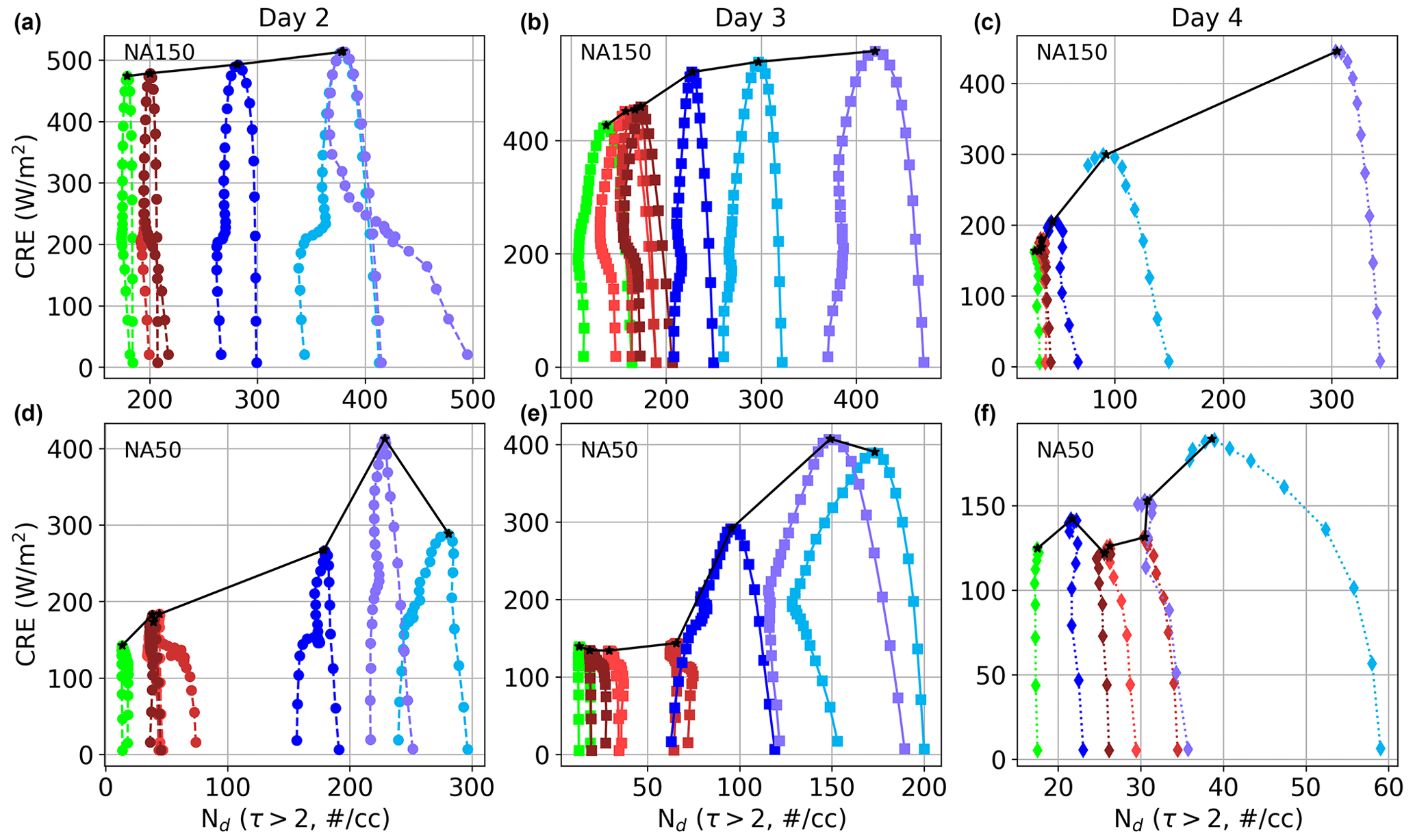
Figure 13CRE vs. Nd for each day in NA150 (a–c) and NA50 (d–f). The color code for the top and bottom panel figures is the same as Figs. 6 and 12, respectively. The separation between consecutive symbols indicates a time difference of 24 min. The black line connects the maximum values in CRE for each case.
4.2 MCB and SCT
These insights indicate that if one considers deliberate injections of aerosol into NEP clouds where precipitation is not imminent (moderately to very polluted clouds), the focus should be to inject as many aerosol particles as possible into the MBL (until coagulation losses start to dominate; see Baker and Charlson, 1990) to enhance the brightness of the cloud deck. The aerosol perturbation should be performed while the ocean surface temperature is relatively cold as advection towards warmer waters strengthens the decoupling of the cloud layer from the surface, which reduces the efficiency of the vertical transport of the injected aerosol. Furthermore, since the spread rate of the aerosol plume is low under these conditions, a more widely distributed injection would aid in a faster dispersal of the injected aerosol. In the context of the pristine system, a high aerosol injection rate is required for a successful implementation of MCB. Since the aerosol plume spread rate in this system is high, the number of sprayers required could be lower. Additionally, if targeted brightening is considered, the pristine system would be more effective due to the substantial enhancement in the CRE due to rapid and strong fc increases soon after aerosol injection ends. However, the frequency of occurrence of such clean boundary layers closer to the coast is very low (Watson-Parris et al., 2021). With the new shipping regulations and a projected reduction in emissions (Westervelt et al., 2015; Diamond, 2023), the frequency of occurrence of such cleaner boundary layers near the coast may increase. In the polluted system, strong changes in CRE are evident only after several hours post-aerosol perturbation. However, combined with their significantly greater frequency of occurrence, the net brightness enhancement from these cloud systems could be substantial. A more systematic analysis is required to confirm this and will be addressed in future studies.
A key question that arises from the results and the discussion here is as follows: to what extent can the SCT be delayed through aerosol perturbations? Additionally, if a substantially higher aerosol concentration is injected into the MBL, would that result in the classic SCT scenario where the transition is due to the warming of the ocean surface and not due to precipitation? The injection of aerosol enhances the colloidal stability of the cloud layer and suppresses precipitation, but it also enhances the entrainment rate of free-tropospheric air, which reduces LWP. However, higher aerosol concentrations deepen the cloud layer and thus have a tendency to enhance LWP (Stevens and Feingold, 2009). The significance of these competing effects may vary on a case-by-case basis. Therefore, a wider variety of simulations under different conditions are required to address these questions.
In this study, we explored how the stratocumulus-to-cumulus transition (SCT) is affected by deliberate aerosol perturbations using a Lagrangian large-eddy simulation (LES) model coupled to a two-moment bulk microphysics scheme. We used the average trajectory from Sandu and Stevens (2011). The setup of these simulations is directed towards marine cloud brightening (MCB) – the deliberate injection of aerosol particles into the marine boundary layer to enhance the brightness of the marine stratocumulus clouds, thereby exerting a cooling effect on the planet. We considered two different baseline aerosol conditions: a polluted (150 particles mg−1) background and a pristine background (50 particles mg−1). We varied the aerosol injection rates per sprayer, number of sprayers, and number of aerosol pulses to assess the impact of various MCB strategies. Our results showed that the spread rate of the aerosol plume is faster in the pristine system due to the transverse circulation induced by the gradient in rain rate across the plume track. In response to the aerosol perturbation, the SCT is delayed in both polluted and pristine systems. To leading order, in the polluted scenario, the time delay in the transition is proportional to the amount of aerosol injected into the MBL and is only weakly affected by the distribution (in space and time) of the aerosol sprayers. The enhancement in cloud radiative effect (CRE) increases from day 2 to day 4. The changes in CRE are dominated by the albedo effect on days 2 and 3 and cloud fraction (fc) adjustments on day 4. In the pristine system, only the strong perturbations make a substantial contribution to MCB. The weak perturbations are dissipated within a day through enhanced precipitation in the aerosol plume track. The time delay in SCT is affected by the total number of aerosol particles injected into the marine boundary layer and their distribution in space and time. A more concentrated but slightly weaker aerosol injection tends to delay the SCT more effectively than splitting it across two sprayers. The enhancement in CRE is dominated by fc and is sustained for 2 d in the strongly perturbed cases.
The results presented here are based on the composite trajectory from a 2-year (2006–2007, June–August) climatology. This average trajectory may mask the variability in profiles, which may impact the SCT. For instance, faster advection or a faster SST increase may result in an early transition. In such a scenario, the time required for the aerosol plume to spread and the corresponding cloud adjustment timescales may affect the effectiveness of MCB. In other words, a different aerosol injection rate and sprayer configuration may be required under these conditions for the effective implementation of MCB. Thus, future studies should use more realistic conditions based on instantaneous soundings and forcings. Additionally, the current Lagrangian model does not account for the large-scale feedback associated with aerosol perturbation. Thus, further model improvements are warranted to better constrain the impact of aerosol perturbation (Chun et al., 2022).
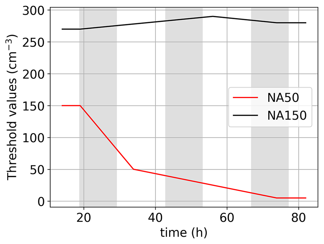
The aerosol plume is detected by setting a threshold manually on the vertically integrated (0 ≤ z ≤ zi) aerosol concentration. For each of the baseline systems (NA150 and NA50), the same threshold values are used in all the perturbed cases. In the NA150 case, the background aerosol concentration has a variability of ±10 % about the mean value. We use a spatial Gaussian filter of five pixels width to smooth these fluctuations. This causes artificial broadening of the plume during its initial evolution period. However, with time, the effect of the filter is weakened due to the increase in plume area coverage. In the NA50 system, the signal-to-noise ratio is very high, even for the weak perturbations (1×). Thus, no filtering is used in determining the plume area coverage in NA50. The time series of the threshold values used in this study is shown in Fig. A1. The threshold values change with time due to the changes in the background conditions. In the NA150 system, the threshold value is nearly constant, with minor (within 15 % of the start value) changes during the evolution of the system. On the other hand, in the NA50 system, the threshold value decreases quickly with time to account for the losses from precipitation in the region away from the plume track. Since the threshold values are the same for all the aerosol plume tracks in each system, a sensitivity test on these threshold is not required as the relative trend in the spread rates would be similar.
The simulations were carried out using SAM (Khairoutdinov and Randall, 2003), which is publicly available at the Harvard repository (https://wiki.harvard.edu/confluence/display/climatemodeling/SAM, Khairoutdinov, 2024). The data from the simulations are available from the NOAA Chemical Sciences Laboratory's Clouds, Aerosol, & Climate program at https://csl.noaa.gov/groups/csl9/datasets/data/cloud_phys/2023-Prabhakaran-etal/ (Prabhakaran, 2023).
PP, FH, and GF designed the research. PP carried out the simulations and analysis. PP, FH, and GF discussed the results. PP wrote the manuscript with input from FH and GF.
At least one of the (co-)authors is a member of the editorial board of Atmospheric Chemistry and Physics. The peer-review process was guided by an independent editor, and the authors also have no other competing interests to declare.
Publisher’s note: Copernicus Publications remains neutral with regard to jurisdictional claims made in the text, published maps, institutional affiliations, or any other geographical representation in this paper. While Copernicus Publications makes every effort to include appropriate place names, the final responsibility lies with the authors.
Marat Khairoutdinov graciously provided the SAM model. Jianhao Zhang, CIRES/NOAA-CSL, provided the data for Fig. 1.
This research has been supported by the U.S. Department of Commerce (Earth's Radiation Budget grant, NOAA CPO Climate & CI (grant no. 03-01-07-001) and NOAA Cooperative Agreement with CIRES (grant no. NA17OAR4320101)) and the Emmy Noether program of the German Research Foundation (Deutsche Forschungsgemeinschaft, DFG (grant no. HO 6588/1-1)).
This paper was edited by Hailong Wang and reviewed by two anonymous referees.
Ackerman, A. S., Stevens, B., Savic-Jovcic, V., Bretherton, C. S., Chlond, A., Golaz, J. C., Jiang, H., Khairoutdinov, M., Krueger, S. K., Lewellen, D. C., and Lock, A.: Large-eddy simulations of a drizzling, stratocumulus-topped marine boundary layer, Mon. Weather Rev., 137, 1083–1110, 2009. a
Ahlm, L., Jones, A., Stjern, C. W., Muri, H., Kravitz, B., and Kristjánsson, J. E.: Marine cloud brightening – as effective without clouds, Atmos. Chem. Phys., 17, 13071–13087, https://doi.org/10.5194/acp-17-13071-2017, 2017. a
Albrecht, B. A.: Aerosols, cloud microphysics, and fractional cloudiness, Science, 245, 1227–1230, 1989. a
Baker, M. B. and Charlson, R. J.: Bistability of CCN concentrations and thermodynamics in the cloud-topped boundary layer, Nature, 345, 142–145, 1990. a
Bretherton, C.: A conceptual model of the stratocumulus-trade-cumulus transition in the subtropical oceans, in: Proceedings of the 11th International Conference on Clouds and Precipitation, 17–21 August 1992, Montreal, PQ, Canada, International Commission on Clouds and Precipitation, vol. 1, 374–377, https://www.google.com/url?sa=t&rct=j&q=&esrc=s &source=web&cd=&cad=rja&uact=8&ved=2ahUKEwjY9but3 aeEAxULxTgGHRhDBzEQFnoECA8QAQ&url=https%3A %2F%2Fwww.iamas.org%2Ficcp%2Fwp-content%2F uploads%2Fsites%2F3%2F2021%2F01%2F11th-Internation-Conference-on-Clouds-and-Precipitation-Proceedings-Vol-I.pdf&usg=AOvVaw0dh-5QnZxuc1yfjDzwZoXl&opi=89978449 (last access: 12 February 2024), 1992. a, b
Bretherton, C., Blossey, P. N., and Uchida, J.: Cloud droplet sedimentation, entrainment efficiency, and subtropical stratocumulus albedo, Geophys. Res. Lett., 34, L03813, https://doi.org/10.1029/2006GL027648, 2007. a, b
Bretherton, C. S. and Blossey, P. N.: Low cloud reduction in a greenhouse-warmed climate: Results from Lagrangian LES of a subtropical marine cloudiness transition, J. Adv. Model. Earth Syst., 6, 91–114, 2014. a
Bretherton, C. S. and Pincus, R.: Cloudiness and marine boundary layer dynamics in the ASTEX Lagrangian experiments. Part I: Synoptic setting and vertical structure, J. Atmos. Sci., 52, 2707–2723, 1995. a
Bretherton, C. S. and Wyant, M. C.: Moisture transport, lower-tropospheric stability, and decoupling of cloud-topped boundary layers, J. Atmos. Sci., 54, 148–167, 1997. a, b
Bretherton, C. S., McCoy, I. L., Mohrmann, J., Wood, R., Ghate, V., Gettelman, A., Bardeen, C. G., Albrecht, B. A., and Zuidema, P.: Cloud, aerosol, and boundary layer structure across the Northeast Pacific stratocumulus–cumulus transition as observed during CSET, Mon. Weather Rev., 147, 2083–2103, 2019. a
Chun, J.-Y., Wood, R., Blossey, P. N., and Doherty, S. J.: The impact of aerosol injections and adjustments in large-scale subsidence on stratocumulus-to-cumulus transition, in: AGU Fall Meeting Abstracts, 12–16 December 2022, Chicago, USA, vol. 2022, A12G-07, 2022. a
Chun, J.-Y., Wood, R., Blossey, P., and Doherty, S. J.: Microphysical, macrophysical, and radiative responses of subtropical marine clouds to aerosol injections, Atmos. Chem. Phys., 23, 1345–1368, https://doi.org/10.5194/acp-23-1345-2023, 2023. a, b, c, d
Clark, T. L.: Numerical modeling of the dynamics and microphysics of warm cumulus convection, J. Atmos. Sci., 30, 857–878, 1973. a
Diamond, M. S.: Detection of large-scale cloud microphysical changes within a major shipping corridor after implementation of the International Maritime Organization 2020 fuel sulfur regulations, Atmos. Chem. Phys., 23, 8259–8269, https://doi.org/10.5194/acp-23-8259-2023, 2023. a
Diamond, M. S., Director, H. M., Eastman, R., Possner, A., and Wood, R.: Substantial cloud brightening from shipping in subtropical low clouds, AGU Advances, 1, e2019AV000111, https://doi.org/10.1029/2019AV000111, 2020. a
Eastman, R. and Wood, R.: Factors controlling low-cloud evolution over the eastern subtropical oceans: A Lagrangian perspective using the A-Train satellites, J. Atmos. Sci., 73, 331–351, 2016. a
Eastman, R., McCoy, I. L., and Wood, R.: Environmental and internal controls on Lagrangian transitions from closed cell mesoscale cellular convection over subtropical oceans, J. Atmos. Sci., 78, 2367–2383, 2021. a
Erfani, E., Blossey, P., Wood, R., Mohrmann, J., Doherty, S. J., Wyant, M., and O, K.-T.: Simulating Aerosol Lifecycle Impacts on the Subtropical Stratocumulus-to-Cumulus Transition Using Large-Eddy Simulations, J. Geophys. Res.-Atmos., 127, e2022JD037258, https://doi.org/10.1029/2022JD037258, 2022. a, b
Feingold, G., Walko, R., Stevens, B., and Cotton, W.: Simulations of marine stratocumulus using a new microphysical parameterization scheme, Atmos. Res., 47, 505–528, 1998. a, b, c
Feingold, G., Koren, I., Yamaguchi, T., and Kazil, J.: On the reversibility of transitions between closed and open cellular convection, Atmos. Chem. Phys., 15, 7351–7367, https://doi.org/10.5194/acp-15-7351-2015, 2015. a, b
Feingold, G., Goren, T., and Yamaguchi, T.: Quantifying albedo susceptibility biases in shallow clouds, Atmos. Chem. Phys., 22, 3303–3319, https://doi.org/10.5194/acp-22-3303-2022, 2022. a
Goren, T. and Rosenfeld, D.: Decomposing aerosol cloud radiative effects into cloud cover, liquid water path and Twomey components in marine stratocumulus, Atmos. Res., 138, 378–393, 2014. a
Goren, T., Kazil, J., Hoffmann, F., Yamaguchi, T., and Feingold, G.: Anthropogenic air pollution delays marine stratocumulus breakup to open cells, Geophys. Res. Lett., 46, 14135–14144, 2019. a
Goren, T., Feingold, G., Gryspeerdt, E., Kazil, J., Kretzschmar, J., Jia, H., and Quaas, J.: Projecting stratocumulus transitions on the albedo–cloud fraction relationship reveals linearity of albedo to droplet concentrations, Geophys. Res. Lett., 49, e2022GL101169, https://doi.org/10.1029/2022GL101169, 2022. a, b, c, d
Hartmann, D. L. and Short, D. A.: On the use of earth radiation budget statistics for studies of clouds and climate, J. Atmos. Sci., 37, 1233–1250, 1980. a
Haywood, J. M., Jones, A., Jones, A. C., and Rasch, P. J.: Climate Intervention using marine cloud brightening (MCB) compared with stratospheric aerosol injection (SAI) in the UKESM1 climate model, EGUsphere [preprint], https://doi.org/10.5194/egusphere-2023-1611, 2023. a
Hoffmann, F. and Feingold, G.: Cloud microphysical implications for marine cloud brightening: The importance of the seeded particle size distribution, J. Atmos. Sci., 78, 3247–3262, 2021. a
Hoffmann, F. and Feingold, G.: A Note on Aerosol Processing by Droplet Collision-Coalescence, Geophys. Res. Lett., 50, e2023GL103716, https://doi.org/10.1029/2023GL103716, 2023. a
Jenkins, A. K. L., Forster, P. M., and Jackson, L. S.: The effects of timing and rate of marine cloud brightening aerosol injection on albedo changes during the diurnal cycle of marine stratocumulus clouds, Atmos. Chem. Phys., 13, 1659–1673, https://doi.org/10.5194/acp-13-1659-2013, 2013. a, b
Kazil, J., Wang, H., Feingold, G., Clarke, A. D., Snider, J. R., and Bandy, A. R.: Modeling chemical and aerosol processes in the transition from closed to open cells during VOCALS-REx, Atmos. Chem. Phys., 11, 7491–7514, https://doi.org/10.5194/acp-11-7491-2011, 2011. a
Kessler, E.: On the distribution and continuity of water substance in atmospheric circulations, in: On the distribution and continuity of water substance in atmospheric circulations, Springer, 1–84, https://doi.org/10.1007/978-1-935704-36-2_1, 1969. a
Khairoutdinov, M.: SAM, Harvard repository [code], https://wiki.harvard.edu/confluence/display/climatemodeling/SAM, last access: 11 February 2024. a
Khairoutdinov, M. and Kogan, Y.: A new cloud physics parameterization in a large-eddy simulation model of marine stratocumulus, Mon. Weather Rev., 128, 229–243, 2000. a
Khairoutdinov, M. F. and Randall, D. A.: Cloud resolving modeling of the ARM summer 1997 IOP: Model formulation, results, uncertainties, and sensitivities, J. Atmos. Sci., 60, 607–625, 2003. a, b
Klein, S. A. and Hartmann, D. L.: The seasonal cycle of low stratiform clouds, J. Climate, 6, 1587–1606, 1993. a
Krueger, S. K., McLean, G. T., and Fu, Q.: Numerical simulation of the stratus-to-cumulus transition in the subtropical marine boundary layer. Part II: Boundary-layer circulation, J. Atmos. Sci., 52, 2851–2868, 1995. a, b, c
Latham, J. and Smith, M.: Effect on global warming of wind-dependent aerosol generation at the ocean surface, Nature, 347, 372–373, 1990. a
Mlawer, E. J., Taubman, S. J., Brown, P. D., Iacono, M. J., and Clough, S. A.: Radiative transfer for inhomogeneous atmospheres: RRTM, a validated correlated-k model for the longwave, J. Geophys. Res.-Atmos., 102, 16663–16682, 1997. a
Paluch, I. and Lenschow, D.: Stratiform cloud formation in the marine boundary layer, J. Atmos. Sci., 48, 2141–2158, 1991. a
Possner, A., Wang, H., Wood, R., Caldeira, K., and Ackerman, T. P.: The efficacy of aerosol–cloud radiative perturbations from near-surface emissions in deep open-cell stratocumuli, Atmos. Chem. Phys., 18, 17475–17488, https://doi.org/10.5194/acp-18-17475-2018, 2018. a
Prabhakaran, P.: Index of/groups/csl9/datasets/data/cloud_phys/2023-Prabhakaran-etal, NOAA Chemical Sciences Laboratory (CSL) [data set], https://csl.noaa.gov/groups/csl9/datasets/data/cloud_phys/2023-Prabhakaran-etal/, last access: 21 July 2023. a
Prabhakaran, P., Hoffmann, F., and Feingold, G.: Evaluation of Pulse Aerosol Forcing on Marine Stratocumulus Clouds in the Context of Marine Cloud Brightening, J. Atmos. Sci., 80, 1585–160, https://doi.org/10.1175/JAS-D-22-0207.1, 2023. a, b, c, d, e, f, g, h
Rasch, P. J., Latham, J., and Chen, C.-C. J.: Geoengineering by cloud seeding: influence on sea ice and climate system, Environ. Res. Lett., 4, 045112, https://doi.org/10.1088/1748-9326/4/4/045112, 2009. a
Sandu, I. and Stevens, B.: On the factors modulating the stratocumulus to cumulus transitions, J. Atmos. Sci., 68, 1865–1881, 2011. a, b, c, d, e, f, g, h
Sandu, I., Brenguier, J.-L., Geoffroy, O., Thouron, O., and Masson, V.: Aerosol impacts on the diurnal cycle of marine stratocumulus, J. Atmos. Sci., 65, 2705–2718, 2008. a
Sandu, I., Stevens, B., and Pincus, R.: On the transitions in marine boundary layer cloudiness, Atmos. Chem. Phys., 10, 2377–2391, https://doi.org/10.5194/acp-10-2377-2010, 2010. a, b, c, d
Sarkar, M., Zuidema, P., Albrecht, B., Ghate, V., Jensen, J., Mohrmann, J., and Wood, R.: Observations pertaining to precipitation within the northeast Pacific stratocumulus-to-cumulus transition, Mon. Weather Rev., 148, 1251–1273, 2020. a
Stevens, B. and Feingold, G.: Untangling aerosol effects on clouds and precipitation in a buffered system, Nature, 461, 607–613, 2009. a
Stjern, C. W., Muri, H., Ahlm, L., Boucher, O., Cole, J. N. S., Ji, D., Jones, A., Haywood, J., Kravitz, B., Lenton, A., Moore, J. C., Niemeier, U., Phipps, S. J., Schmidt, H., Watanabe, S., and Kristjánsson, J. E.: Response to marine cloud brightening in a multi-model ensemble, Atmos. Chem. Phys., 18, 621–634, https://doi.org/10.5194/acp-18-621-2018, 2018. a
Turton, J. and Nicholls, S.: A study of the diurnal variation of stratocumulus using a multiple mixed layer model, Q. J. Roy. Meteor. Soc., 113, 969–1009, 1987. a
Twomey, S.: Pollution and the planetary albedo, Atmos. Environ., 8, 1251–1256, 1974. a
Twomey, S.: The influence of pollution on the shortwave albedo of clouds, J. Atmos. Sci., 34, 1149–1152, 1977. a
Wang, H. and Feingold, G.: Modeling mesoscale cellular structures and drizzle in marine stratocumulus. Part II: The microphysics and dynamics of the boundary region between open and closed cells, J. Atmos. Sci., 66, 3257–3275, 2009a. a, b
Wang, H. and Feingold, G.: Modeling mesoscale cellular structures and drizzle in marine stratocumulus. Part I: Impact of drizzle on the formation and evolution of open cells, J. Atmos. Sci., 66, 3237–3256, 2009b. a, b, c, d
Wang, H., Rasch, P. J., and Feingold, G.: Manipulating marine stratocumulus cloud amount and albedo: a process-modelling study of aerosol-cloud-precipitation interactions in response to injection of cloud condensation nuclei, Atmos. Chem. Phys., 11, 4237–4249, https://doi.org/10.5194/acp-11-4237-2011, 2011. a, b, c
Wang, S., Wang, Q., and Feingold, G.: Turbulence, condensation, and liquid water transport in numerically simulated nonprecipitating stratocumulus clouds, J. Atmos. Sci., 60, 262–278, 2003. a, b
Watson-Parris, D., Sutherland, S., Christensen, M., Eastman, R., and Stier, P.: A large-scale analysis of pockets of open cells and their radiative impact, Geophys. Res. Lett., 48, e2020GL092213, https://doi.org/10.1029/2020GL092213, 2021. a
Westervelt, D. M., Horowitz, L. W., Naik, V., Golaz, J.-C., and Mauzerall, D. L.: Radiative forcing and climate response to projected 21st century aerosol decreases, Atmos. Chem. Phys., 15, 12681–12703, https://doi.org/10.5194/acp-15-12681-2015, 2015. a
Wood, R.: Stratocumulus clouds, Mon. Weather Rev., 140, 2373–2423, 2012. a
Wood, R.: Assessing the potential efficacy of marine cloud brightening for cooling Earth using a simple heuristic model, Atmos. Chem. Phys., 21, 14507–14533, https://doi.org/10.5194/acp-21-14507-2021, 2021. a, b
Wyant, M. C., Bretherton, C. S., Rand, H. A., and Stevens, D. E.: Numerical simulations and a conceptual model of the stratocumulus to trade cumulus transition, J. Atmos. Sci., 54, 168–192, 1997. a, b, c
Yamaguchi, T., Feingold, G., Kazil, J., and McComiskey, A.: Stratocumulus to cumulus transition in the presence of elevated smoke layers, Geophys. Res. Lett., 42, 10–478, 2015. a, b, c
Yamaguchi, T., Feingold, G., and Kazil, J.: Stratocumulus to cumulus transition by drizzle, J. Adv. Model. Earth Syst., 9, 2333–2349, 2017. a, b, c, d, e, f, g, h, i, j
Zhou, X., Ackerman, A. S., Fridlind, A. M., Wood, R., and Kollias, P.: Impacts of solar-absorbing aerosol layers on the transition of stratocumulus to trade cumulus clouds, Atmos. Chem. Phys., 17, 12725–12742, https://doi.org/10.5194/acp-17-12725-2017, 2017. a, b