On the influence of vertical mixing, boundary layer schemes, and temporal emission profiles on tropospheric NO₂ in WRF-Chem – comparisons to in situ, satellite, and MAX-DOAS observations

We present WRF-Chem simulations over central Europe with a spatial resolution of 3 km × 3 km and focus on nitrogen dioxide (NO₂). A regional emission inventory issued by the German Environmental Agency, with a spatial resolution of 1 km × 1 km, is used as input. We demonstrate by comparison of five different model setups that significant improvements in model accuracy can be achieved by choosing the appropriate boundary layer scheme, increasing vertical mixing strength, and/or tuning the temporal modulation of the emission data (“temporal profiles”) driving the model. The model setup with improved vertical mixing is shown to produce the best results. Simulated NO₂ surface concentrations are compared to measurements from a total of 275 in situ measurement stations in Germany, where the model was able to reproduce average noontime NO₂ concentrations with a bias of ca. −3 % and R=0.74. The best agreement is achieved when correcting for the presumed NO_y cross sensitivity of the molybdenum-based in situ measurements by computing an NO_y correction factor from modelled peroxyacetyl nitrate (PAN) and nitric acid (HNO₃) mixing ratios. A comparison between modelled NO₂ vertical column densities (VCDs) and satellite observations from TROPOMI (TROPOspheric Monitoring Instrument) is conducted with averaging kernels taken into account. Simulations and satellite observations are shown to agree with a bias of +5.5 % and R=0.87 for monthly means. Lastly, simulated NO₂ concentration profiles are compared to noontime NO₂ profiles obtained from multi-axis differential optical absorption spectroscopy (MAX-DOAS) measurements at five locations in Europe. For stations within Germany, average biases of −25.3 % to +12.0 % were obtained. Outside of Germany, where lower-resolution emission data were used, biases of up to +50.7 % were observed. Overall, the study demonstrates the high sensitivity of modelled NO₂ to the mixing processes in the boundary layer and the diurnal distribution of emissions.

1 Introduction

Modelling of regional atmospheric chemistry and transport (RCT) is an important discipline in the field of air quality research. While observational data are often only available at coarse spatial or temporal resolutions, model data can be generated on regular grids of much higher spatiotemporal resolution. Modern RCT models can therefore be used to systematically investigate the processes of transport and (photo)-chemical conversion that trace gases are subject to upon emission into the atmosphere. Most importantly, however, they allow for predictions of trace gas concentrations when observational data are not available for operational air quality forecasting. Thus, they give valuable insight into the dynamics of air quality in polluted regions of the Earth. Examples for state-of-the-art RCT models are WRF-Chem (Grell et al., 2005), COSMO/MESSy (Kerkweg and Jöckel, 2012), Lotos-Euros (Manders et al., 2017), CAM-chem (Emmons et al., 2020), and CHIMERE (Menut et al., 2021).

Nitrogen dioxide (NO₂) is one of the most relevant chemical species for air quality in polluted regions. It is toxic to humans and acts as a precursor for ozone (O₃), a key pollutant of urban smog. The hazardous impact of NO₂ on human health has been widely recognized among the scientific community (see, e.g. Faustini et al., 2014; Mills et al., 2015; Chowdhury et al., 2021). Monitoring and predicting realistic distributions of NO₂ in the troposphere is therefore of ongoing political and scientific interest.

Past modelling efforts with focus on tropospheric NO₂ have typically resulted in very similar general outcomes: while researchers found good agreement between modelled and observed meteorological data (such as wind speeds and air temperature), systematic disagreements between modelled surface NO₂ concentrations and in situ observations were found. Visser et al. (2019) report on the results of a WRF-Chem simulation using the Carbon Bond Mechanism Z (CBM-Z) over central Europe in which noontime NO₂ surface concentrations and vertical column densities (VCDs) were underestimated by 38.5 % and approximately 15 %, respectively. In a comparison of monthly mean NO₂ VCDs, R values between 0.82 and 0.92 were obtained. The authors identify an underestimation of soil emissions in their emission inventory (TNO-MACC-III, short for “Monitoring Atmospheric Composition and Climate” by the Netherlands Organisation for Applied Scientific Research) as a possible explanation. Kuik et al. (2016) present a WRF-Chem simulation with the Regional Acid Deposition Model 2 (RADM2) and the same emission inventory as Visser et al. (2019) over the region of Berlin, Germany, and observe even stronger underestimations of surface NO₂ by more than 50 % during daytime and a strong overestimation at night-time in a similar comparison. The study reveals that increasing the spatial resolution (including downscaling of emission data) of the model from 15 km × 15 km to 1 km × 1 km slightly improves agreement but not to a satisfying degree. In a subsequent publication (Kuik et al., 2018), the authors attribute the disagreements to underestimations in the emission data. Poraicu et al. (2023) show a WRF-Chem simulation with the CBM-Z mechanism over a domain in Belgium, where simulated NO₂ showed daytime underestimations of up to 25.1 % and night-time overestimations of up to 77.3 %. The authors experiment with the choice of the boundary layer scheme, as well as a correction factor for cross sensitivities of the reference in situ measurements to other nitrogen compounds. Although slight improvements were achieved, the described model bias persists. Du et al. (2020) demonstrate that tuning the vertical mixing parameterization of different boundary layer schemes in WRF-Chem drastically reduces model biases (shown for PM_2.5 over China), particularly at night-time during summer months. Mar et al. (2016) study the influence of the chemical mechanism on modelled O₃ and NO₂ by direct comparison of the mechanisms MOZART (Model for Ozone and Related chemical Tracers) and RADM2. While the two mechanisms were found to produce significantly different results for O₃, the differences in modelled NO₂ were much smaller. On average, the NO₂ concentrations obtained from MOZART were 2 µg m⁻³ larger than those obtained from RADM2. However, a study based on box model simulations by Knote et al. (2015) reveals much larger discrepancies between chemical mechanisms of up to 25 % for NO_x and 100 % for NO₃, which plays a significant role in night-time NO_x chemistry. Furthermore, some chemical mechanisms were found to be outdated, e.g. with respect to organic nitrate chemistry.

Kumar et al. (2021) demonstrate in a simulation with the MECO(n) model system over Germany using a mixture of TNO-MACC-III and regional emission data that agreement between modelled NO₂ concentrations and in situ observations improves greatly when diurnal and seasonal variability is added to the yearly resolved emission data using hourly and monthly weighting factors (“temporal profiles”). This temporal upsampling has become common practice among the air quality modelling community, and standard values for such temporal profiles have been established (see Crippa et al., 2020b; Kumar et al., 2021, and the references within). Based on their efforts to reduce model bias by other means, Poraicu et al. (2023) conclude that the mismatch between modelled and observed diurnal cycle of surface NO₂ could relate to faulty diurnal emission profiles and/or to insufficient vertical mixing during the night.

A number of publications show that the observed daytime low bias of modelled surface NO₂ could relate to systematic flaws in the ground based in situ measurements used as reference. Conventional in situ methods often utilize molybdenum converters, which were found to be cross sensitive to other reactive nitrogen species, such as peroxyacetyl nitrate (PAN), nitric acid (HNO₃), and alkyl nitrates, summarized as NO_y. This issue was discussed, e.g. by Dunlea et al. (2007), Steinbacher et al. (2007), Lamsal et al. (2008), Boersma et al. (2009), and Villena et al. (2012), who found biases reaching up to a factor of 4 with a strong correlation to O₃ (which again correlates with photochemical activity). Poraicu et al. (2023) attempt to account for such cross sensitivities by computing a correction factor based on simulated surface mixing ratios of PAN and HNO₃. The method contributes to resolving the daytime low bias of the model but is not helpful with respect to the even larger high bias at night-time. In Europe, in situ measurements of NO₂ must conform to regulations defined by the European Norms 14221, 14181, and 15267, which require empirical evidence that the instrument in question is unbiased against direct (e.g. spectroscopic) measurements of NO₂. Such conformity assessments are conducted and thoroughly protocolled by technical inspection associations (such as the TÜV for the in situ measurements in Germany, which are used in this article, see German Environmental Agency, 2023). There is a clear conflict between the overestimations reported in the scientific literature and the proclaimed conformance to the European regulations, and the true magnitude of the problem remains up for debate.

The contemporary literature comes to a clear consensus: surface NO₂ concentrations in RCT simulations are typically underestimated at daytime and overestimated at night-time. The phenomenon was observed consistently across different combinations of geographical domains, model resolutions, emission inventories, boundary layer schemes, chemical mechanisms, and reference data sources used in the past (see Visser et al., 2019; Kuik et al., 2016, 2018; Poraicu et al., 2023). Comparisons to other observational datasets (mainly satellite observations) do occur in the literature and generally show better agreement. However, satellite measurements often yield only a single measurement of the vertically integrated concentration per day; i.e. they do not cover the diurnal cycle.

In this paper, we show the results of a WRF-Chem simulation over central Europe for the month of May 2019 with a spatial resolution of 3 km × 3 km. The goal is to quantify the level of agreement between simulated NO₂ concentrations and VCDs and the corresponding results from different observational datasets. For this purpose our simulation results are compared to the following three reference datasets.

• 1.

  Surface NO₂ concentrations measured by a network of in situ instruments over Germany, operated by the German Environmental Agency (UBA; see German Environmental Agency, 2022).

• 2.

  Tropospheric NO₂ VCDs measured by TROPOMI (TROPOspheric Monitoring Instrument) on the Sentinel 5 precursor satellite, specifically the processor version 20400. This includes recomputing the air mass factors (AMFs) of the retrieval based on our simulation results.

• 3.

  NO₂ concentration profiles obtained from five multi-axis differential optical absorption spectroscopy (MAX-DOAS) instruments that partake in the FRM4DOAS project (see Fayt et al., 2021)

In the scope of a sensitivity analysis, we test whether the model bias observed in the diurnal cycle of surface NO₂ can be resolved by any of the following processes (or a combination thereof):

• 1.

  correcting for the NO_y cross sensitivity of the UBA in situ measurements, based on modelled PAN and HNO₃;

• 2.

  comparing different boundary and surface layer schemes;

• 3.

  implementing tuned mixing, as proposed by Du et al. (2020);

• 4.

  tuning the temporal emission profiles of the most dominant emission sectors.

The article is structured as follows: Sect. 2 describes the different setups of our WRF-Chem simulation and the preprocessing of emission data in detail. Section 3 compares the individual model runs to each other and the above-mentioned observational datasets. Possible explanations for the observed differences are given from a technical perspective. Section 4 presents a conclusion and discussion of the results.

2 WRF-Chem simulation setup

WRF-Chem (Weather Research and Forecasting model with Chemistry; see Grell et al., 2005) is a mesoscale RCT model. We ran WRF-Chem version 4.2.2 on a 2-fold nested domain over central Europe for the month of May 2019; see Fig. 1. The spatial resolutions of the outer and inner domain (called D1, and D2 from hereon) are 15 km × 15 km and 3 km × 3 km (with 320×245 and 500×430 pixels, respectively). The temporal resolution of the simulation is 60 s on D1 and 12 s on D2. Output files are written daily for D1 and hourly for D2.

The simulation uses the Thompson microphysics scheme (see Thompson et al., 2008), the RRTMG (Rapid Radiative Transfer Model for General Circulation Models longwave and shortwave radiation scheme; see Iacono et al., 2008), the Monin–Obukhov similarity scheme for surface layer modelling (see Monin and Obukhov, 1954), the NOAH Land-Surface Model (see Niu et al., 2011), the YSU boundary layer scheme (see Hong, 2010), and the Grell–Dévényi ensemble scheme for cumulus modelling (see Grell and Dévényi, 2002). For modelling of chemistry, the MOZART-4 chemical mechanism (see Emmons et al., 2010) is coupled to the GOCART aerosol mechanism (see Chin et al., 2000) along with the TUV full photolysis scheme (Madronich, 1987; Tie et al., 2003), which deploys climatological O₃ and O₂ columns. Dry deposition is calculated according to Wesely (1989). Spectral nudging (see, e.g. Omrani et al., 2012) to ERA5 reanalysis data (see Hersbach and Dee, 2017) is used on D1. The simulation uses a total of 43 vertical levels in terrain-following coordinates (see Table A1 for the layer heights up to 6 km). Both domains D1 and D2 receive initial conditions from the CAM-chem model (Emmons et al., 2020). Additionally, CAM-chem yields the boundary conditions for D1. D2 receives boundary conditions online from the WRF-Chem simulation running on D1. We refer to this base model setup as “S-YSU”.

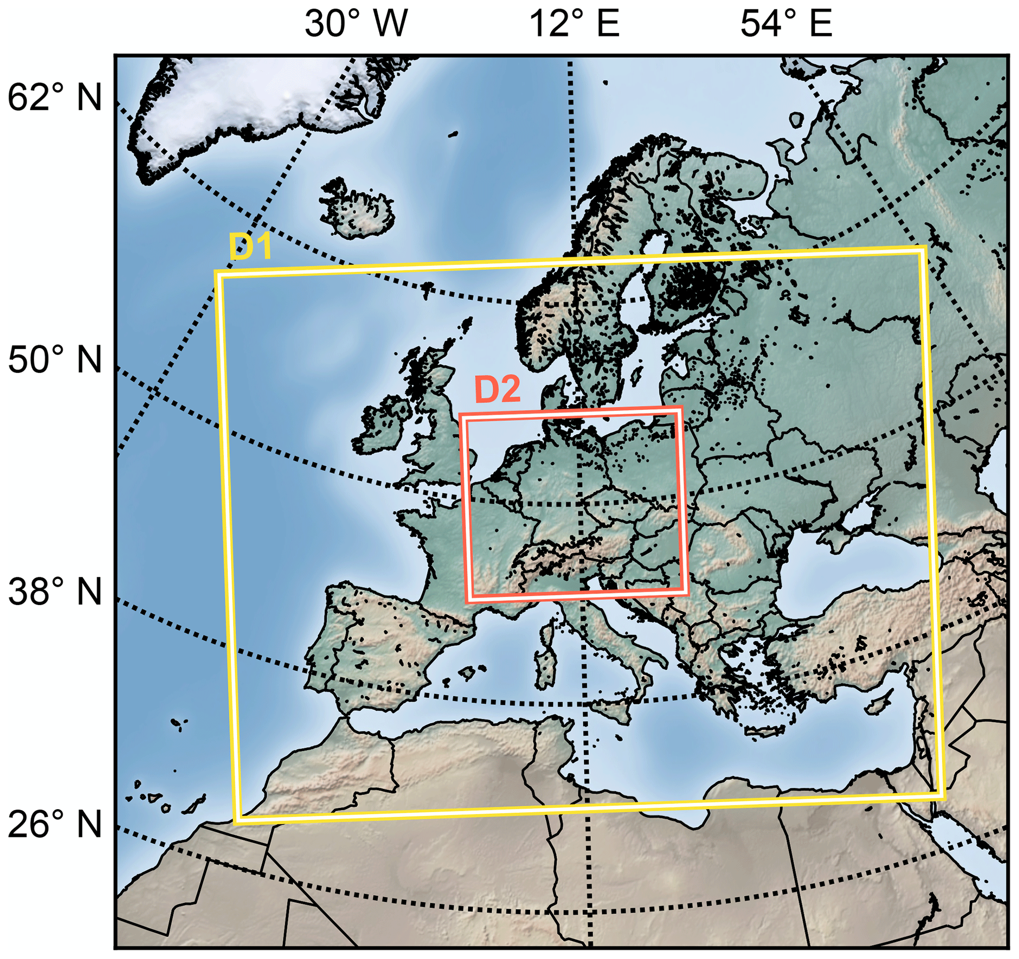
Figure 1 Geographical coverage of the WRF-Chem simulation. The spatial resolutions of the outer domain D1 and the inner domain D2 are 15 km × 15 km, and 3 km × 3 km, respectively.

2.1 Emission preprocessing

The WRF-Chem simulation is driven by different emission inventories for different emission sectors. Emissions from biomass burning are taken from the Fire Inventory from NCAR (FINN; see Wiedinmyer et al., 2011) with a spatiotemporal resolution of 1 km × 1 km and 24 h. Biomass burning emissions are assumed to have a diurnal variation with a peak in the early afternoon (13:00 UTC, coordinated universal time; the time zone for all instances in the text is UTC) and are distributed vertically in the model following the plume rise parameterization of Freitas et al. (2007). Biogenic emissions are computed online using an implementation of the MEGAN model (see Guenther et al., 2006). For anthropogenic emissions a combination of two emission inventories is used. Over Germany, an inventory of high spatial resolution (1 km × 1 km, resampled to 0.01^∘ × 0.01^∘ or ∼ 1.1 km × 0.7 km) is provided by the UBA (see Strogies et al., 2020). From hereon, this emission inventory will be referenced as UBA-E. Using the UBA-E emission data over Germany enables modelling of NO₂ distributions at a high spatial resolution. Outside of Germany, the EDGARv5 emission inventory with a moderate spatial resolution (0.1^∘ × 0.1^∘ or ∼ 11 km × 7 km) is used (see Crippa et al., 2020a). Since UBA-E does not include organic anthropogenic emissions, EDGARv5 is used on the entirety of D1 and D2 for organic species. Non-methane volatile organic compounds (NMVOCs) are provided as lumped species and are speciated according to Huang et al. (2017). An alternative to EDGARv5 would have been the TNO-MAC-III emission inventory (Kuenen et al., 2014), which comes at a higher spatial resolution of 0.0625^∘ × 0.125^∘ but was only available for the year 2011 at the time the simulation was run. Since EDGARv5 was available for 2015 and NO_x emissions have steadily decreased over the past years (see, e.g. Anenberg et al., 2022), EDGARv5 was considered a more reasonable choice.

EDGARv5 (for 2015) and UBA-E have time resolutions of 1 month and 1 year, respectively. However, many emissions follow strong diurnal and seasonal patterns. For example, emissions from car traffic are expected to be lower at night-time and higher at daytime, and agricultural emissions typically occur in specific months of the year. EDGARv5 can still resolve emission variations on a monthly time resolution but is incapable of resolving diurnal patterns. UBA-E provides only annual emissions and therefore is without any temporal pattern. The solution to this problem is to scale the coarsely resolved emission data to an hourly resolution using presumed hourly, daily, and monthly emission scaling factors (temporal profiles). The emission rate $E_{X,k}(m,d,h,\text{lat},\text{long})$ of a species X from sector k at month m, day d, and hour h at fixed latitude (lat) and longitude (long) is given as follows:

$$\begin{array}{}\text{(1)}& \begin{array}{rl}{E}_{X,k}(m,d,h,\text{lat},\text{long})& ={\widehat{E}}_{X,k}(\text{lat},\text{long})\cdot p_{\mathrm{monthly},k}\left(m\right)\\ & \cdot p_{\mathrm{daily},k}\left(d\right)\cdot p_{\mathrm{hourly},k}\left(h\right),\end{array}\end{array}$$

where ${\widehat{E}}_{X,k}$ denotes the total emissions of species X from sector k in the emission inventory and p_monthly, p_daily, and p_hourly the monthly, daily, and hourly temporal profiles. The individual profiles are normalized to 12 (annual cycle), 7 (weekly cycle), and 24 (diurnal cycle), respectively. Because different emission sectors follow vastly different temporal patterns, the temporal profiles are defined for each sector individually. An overview of the emission sectors is given in Table 1. The total emission rate of species X is obtained by summation over all emission sectors k as follows:

$$\begin{array}{}\text{(2)}& \begin{array}{rl}{E}_X(m,d,h,\text{lat},\text{long})& =\sum _k{\widehat{E}}_{X,k}(\text{lat},\text{long})\cdot p_{\mathrm{monthly},k}\left(m\right)\\ & \cdot p_{\mathrm{daily},k}\left(d\right)\cdot p_{\mathrm{hourly},k}\left(h\right).\end{array}\end{array}$$

Some species are only implicitly contained in the emission inventories. For example, EDGARv5 and UBA-E specify NO_x emissions, but the partitioning into NO and NO₂ must be chosen by the user via a speciation profile p_spec. Equation (2) then generalizes to

$$\begin{array}{}\text{(3)}& \begin{array}{rl}{E}_X(m,d,h,\text{lat},\text{long})& =\sum _k{\widehat{E}}_{X_{\mathrm{lump}},k}(\text{lat},\text{long})\\ & \cdot p_{\mathrm{monthly},k}\left(m\right)\cdot p_{\mathrm{daily},k}\left(d\right)\\ & \cdot p_{\mathrm{hourly},k}\left(h\right)\cdot p_{\mathrm{spec},k}\left(X\right)\end{array},\end{array}$$

where X_lump is the lump of species that contains species X (i.e. X_lump=NO_x when X=NO₂).

Table 1 Emission sectors in the UBA-E and EDGARv5 emission inventories.

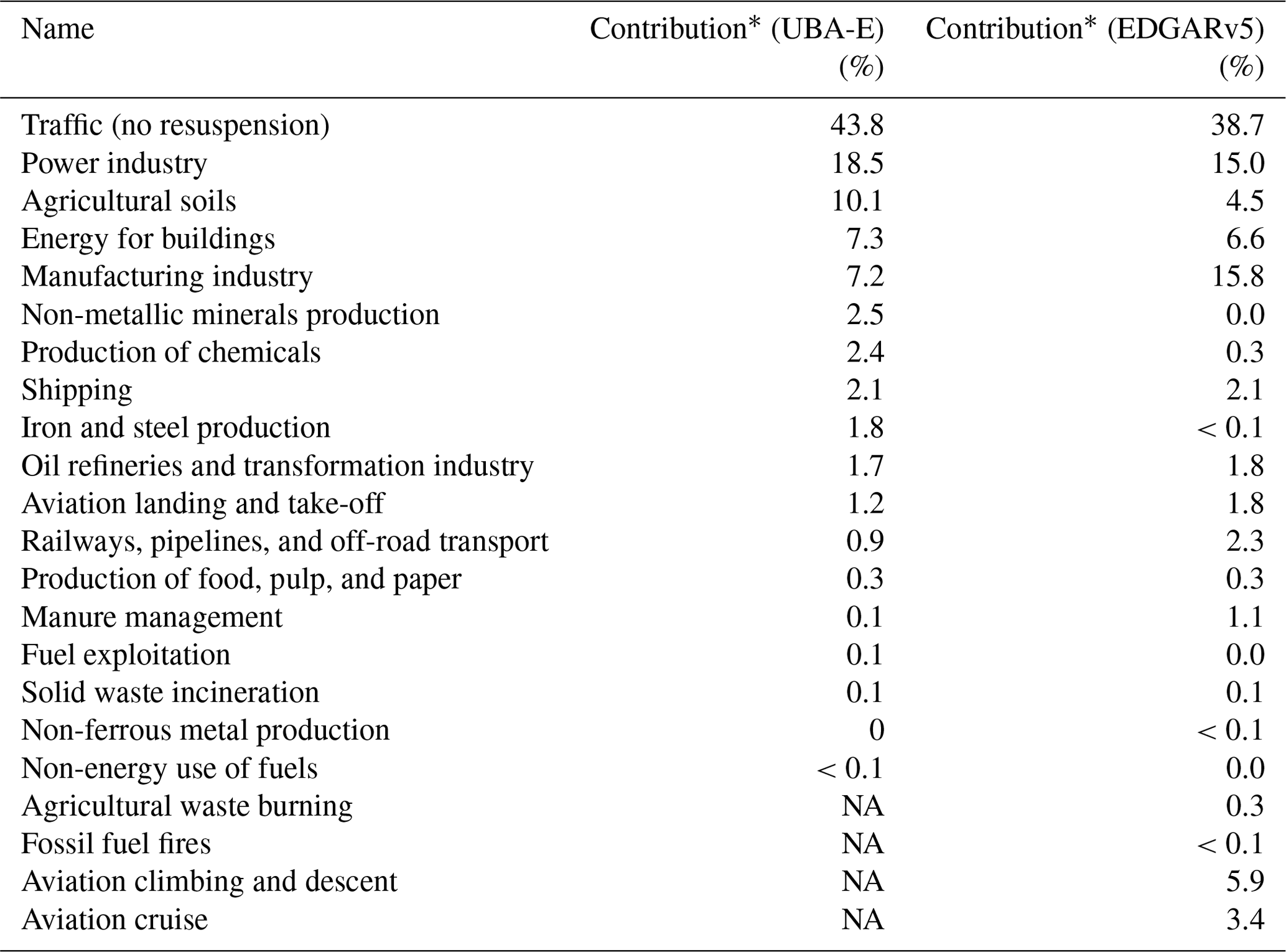
NA stands for not available. ^* Relative contribution of this sector to the overall emissions (yearly for UBA-E and for the month of May for EDGARv5) of NO_x.

In principle, WRF-Chem also supports vertical distribution of trace gas emissions. This is reasonable to consider given that many strong emissions, like those from combustion stacks, take place at elevated altitudes. In analogy to the mentioned temporal and speciation profiles, this can be modelled using an additional vertical emission profile. Suggestions for vertical emission profiles are given in Bieser et al. (2011) and Pozzer et al. (2009). The optimization of vertical emission profiles is not in the scope of our study because the majority of the observational data used (in situ measurements and most satellite observations) stem from background locations, where almost all emissions occur at the surface, and transport and vertical mixing further minimize the influence of height-distributed emissions. Hence, all emissions are injected into the lowest model layer (0–8 m).

2.2 Model variants with different boundary layer and surface layer schemes

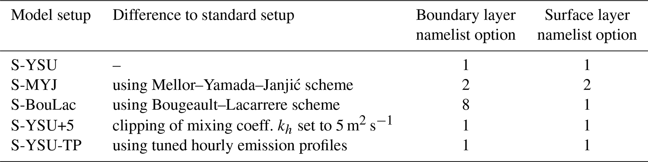
We conduct two additional model runs with different combinations of planetary boundary layer (PBL) and surface layer schemes.

• 1.

  The Mellor–Yamada–Janjić scheme (MYJ; see Mesinger, 1993; Janjić, 1994), coupled with the Monin–Obukhov (Janjić Eta) similarity scheme. We refer to this model setup as “S-MYJ”.

• 2.

  The Bougeault–Lacarrere scheme (BouLac, see Bougeault and Lacarrere, 1989), coupled with the Monin–Obukhov scheme with a Carlson–Boland viscous sub-layer. We refer to this model setup as “S-BouLac”.

This choice of schemes was motivated by the WRF-Chem user guide (which recommends the YSU and MYJ boundary layer schemes; see University Corporation for Atmospheric Research, 2023), as well as the findings of Poraicu et al. (2023), who demonstrate that the BouLac boundary layer scheme tends to produce particularly low NO₂ concentrations at night-time.

2.3 Model variant with tuned vertical mixing

The work of Du et al. (2020) demonstrates that the diurnal cycle of PM_2.5 can be reproduced much more accurately by tuning the vertical mixing within WRF-Chem. Given that PM_2.5 and trace gases are subject to the same mixing routine in WRF-Chem, it is highly plausible that their approach has a similar effect on the diurnal cycle of NO₂.

Mixing in WRF-Chem is computed in two steps: first, a mixing coefficient k_h (called “EXCH_H” in the WRF-Chem registry) is computed by the PBL scheme. Following this, a mixing routine is called, which dilutes the trace gas concentration of each model layer into its neighbours based on the magnitude of k_h. The mixing routine implements a crucial manipulation of k_h: depending on a coarse classification of the model cell as either “rural” or “urban”, k_h is clipped to a minimum of 1 or 2 m² s⁻¹ for the lowest model layers, respectively. This is fundamental with regard to modelling surface concentrations, seeing that the boundary layer schemes shown in Du et al. (2020) (and those shown within this paper) tend to produce mixing coefficients smaller than 1 m² s⁻¹ at the surface, particularly at night-time. In essence, this implementation results in increased vertical mixing, and the effect is strongest during the night. The WRF-Chem source code encourages the user to tune this enhancement further (see the WRF-Chem source code file “chem/dry_dep_driver.F”, where the described mixing procedure is implemented). However, the parameterization is hard-coded and can only be changed by complete recompilation of WRF-Chem. Following the recommendation of Du et al. (2020), we present a model run where the clipping of k_h is enhanced to 5 m² s⁻¹ everywhere. We refer to this model setup as “S-YSU+5”.

2.4 Model variant with tuned diurnal emission profiles

Another approach to reducing the bias of the modelled diurnal NO₂ cycle is to tune the hourly profiles used in the preprocessing of the emission data. The goal is to find temporal profiles that minimize the model's mean NO_x bias over the course of the day. The mean relative bias is computed as

$$\begin{array}{}\text{(4)}& \text{bias}={\displaystyle \frac{\mathrm{1}}{N}}\sum _{i=\mathrm{1}}^N{\displaystyle \frac{x_{\mathrm{sim},i}-x_{\mathrm{obs},i}}{x_{\mathrm{obs},i}}},\end{array}$$

where x_obs, i denotes the ith observation and x_sim, i the corresponding simulated value. We use the observations from in situ measurements of background NO_x surface concentrations as reference. A detailed explanation of the dataset is given in Sect. 3.1. Equation (3) hints towards the complexity of the optimization problem: because the emission inventories include dozens of emission sectors, each with their own emission profiles, this poses an optimization problem with many degrees of freedom. In addition, a single WRF-Chem simulation of just 1 month takes days to finish even on modern supercomputers. This circumstance makes it nearly impossible to optimize the emission profiles using standard methods like gradient descent. For our simulation we have therefore optimized the emission profiles empirically. By “empirical optimization” we mean the iterative process of running WRF-Chem, evaluating the simulation results against in situ observations, and slightly nudging the temporal profiles in a direction in which better agreement between simulation and observations can be expected. Due to the short lifetime of NO_x, the observed concentrations follow the temporal profiles without much delay. As an initial starting point, the temporal profiles from Kumar et al. (2021) were used. Although the proposed optimization method is rather unconventional, it has a few important benefits, including the following aspects.

• 1.

  The hourly profiles of many sectors have characteristic shapes, e.g. a peak in the hourly profile of the traffic sector during the morning rush hour. These should be at least coarsely preserved during the optimization process in order to maintain realistic emission behaviour.

• 2.

  Because the optimization problem is ill-posed, it is often unclear in which sector the profiles should be tuned further in order to improve the simulation. Sometimes the spatial distribution of a specific emission sector matches that of the model error, indicating that this sector should be prioritized.

• 3.

  Gradient-based optimization methods depend on hyperparameters, such as the step size. If these are not picked correctly from the start, the optimization may converge slowly or diverge entirely. This becomes infeasible when a single forward run takes days to compute.

Using a conventional optimization routine, where the gradient of a loss function determines the outcome of a single optimization step, would require us to encode the three above aspects in the form of mathematical constraints. This makes a rigorous treatment of the problem extremely complex. The empirical optimization approach, however, does not require a mathematical formulation and can thus take the discussed aspects into consideration more easily. We run the optimization under the following conditions.

• 1.

  Only the most relevant emission sectors are modified during the process. According to Table 1 these are traffic (no resuspension), the power industry, agricultural soils, energy for buildings, and the manufacturing industry.

• 2.

  Speciation of lumped species follows the recommendations of Huang et al. (2017) and is not further optimized. For NO_x, the partitioning is assumed to be 87.5 % NO and 12.5 % NO₂. This choice reflects the fact that NO_x from combustion processes is mostly emitted as NO, which oxidizes to NO₂ over time. Literature values for typical ${\mathrm{NO}}_{\mathrm{2}}/{\mathrm{NO}}_x$ ratios in anthropogenic emissions range from lower values (e.g. 5.3 %, as reported by Wild et al., 2017, and 7.8 %, as reported by Jimenez et al., 2000) to much higher values (e.g. 39 %, as reported by Richmond-Bryant et al., 2017, and 36 %, as reported by Costantini et al., 2016).

• 3.

  In order to improve generalization of the temporal profiles, the optimization is performed using data from May 2018. Additionally, we accelerate the optimization by only using 2 weeks of simulation time for each optimization step. The final temporal profiles are evaluated in a full-month simulation for the year 2019, as described in Sect. 2.

• 4.

  The NO_y cross sensitivities of the reference measurements are not taken into account during the optimization process. Their influence is described in more detail in Sect. 3.1.

Figure 2 gives an overview of the optimization process in a total of three iterations. The monthly and weekly emission cycle was taken directly from Kumar et al. (2021). Following this, the hourly profiles were adjusted to compensate the model bias. For example, in step 1 (red line), only a single change was made to the traffic sector profile (Fig. 2a) in order to boost simulated NO_x values in the morning (∼ 06:00 LT). The principle was extended to the remaining hourly profiles in the next two steps. We refer to this model setup as “S-YSU-TP”. Table 2 gives an overview of the five different model setups used within our study.

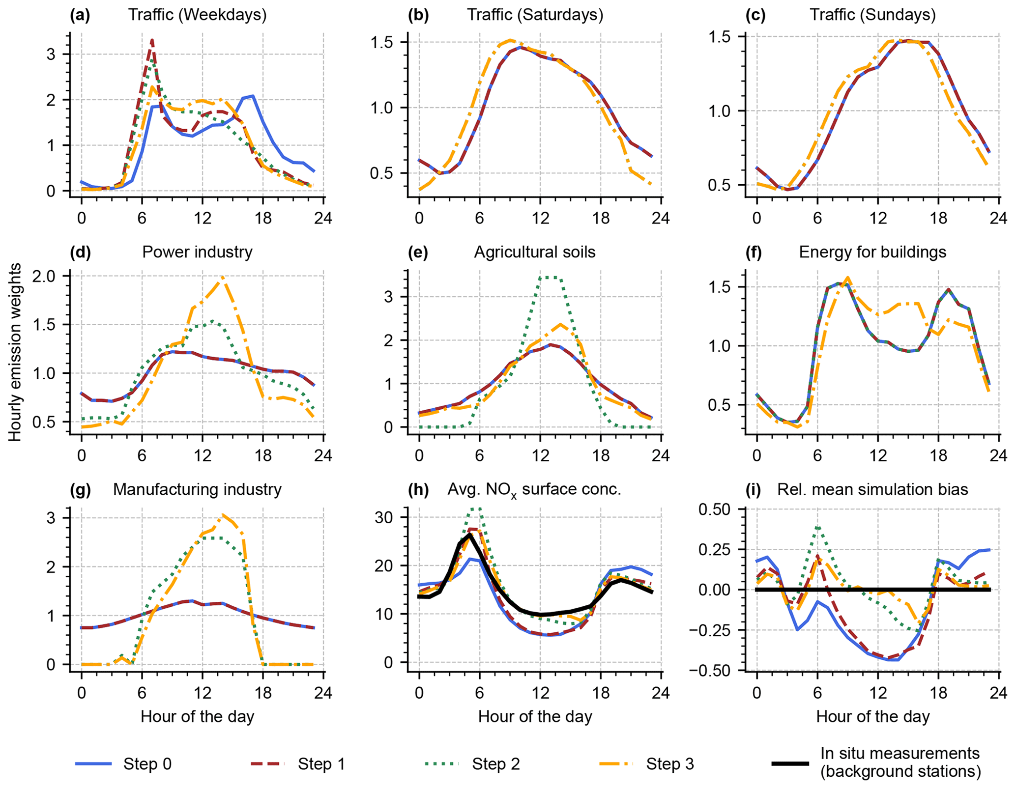
Figure 2 Overview of the optimization process for the diurnal emission profiles based on the in situ observations of May 2018. The profiles used by Kumar et al. (2021) are drawn in blue, and the optimized profiles used in S-YSU-TP are drawn in orange.

Table 2 Overview of the different model setups used within our study.

3 Results

3.1 Comparison of surface concentrations

In situ measurements of trace gas surface concentrations in Germany are conducted by the UBA. They are available for NO₂, NO, and O₃ as hourly mean values. A total of 434 UBA measuring stations are distributed over Germany. A total of 92 % of the stations use a chemiluminescence-based measuring method. The remaining 8 % use other methods (cavity-enhanced phase shift spectroscopy, diffuse sampling, or photolysis conversion). Of all UBA stations, 63 % are classified as “background”, 30 % as “traffic”, and 7 % as “industry”. In this study we only take background stations into consideration. This choice was made seeing that NO₂ concentration can vary strongly near traffic over distances of only 10–100 m (see, e.g. Beckwith et al., 2019) and timescales of a few minutes. Given our simulation's spatial resolution of 3 km × 3 km, it is expected to show poor agreement with the traffic stations.

In order to compare the simulated surface concentrations to the in situ measurements, they are interpolated from the WRF-Chem simulation grid to the geolocations of the UBA stations. As introduced in Sect. 1, the molybdenum-based chemiluminescence method for NO₂ detection is likely cross sensitive to NO_y. We account for this by computing a correction factor

$$\begin{array}{}\text{(5)}& F=\mathrm{1}+{\displaystyle \frac{\mathrm{0.95}\cdot \left[\text{PAN}\right]+\mathrm{0.35}\cdot \left[{\mathrm{HNO}}_{\mathrm{3}}\right]}{\left[{\mathrm{NO}}_{\mathrm{2}}\right]}},\end{array}$$

as proposed by Lamsal et al. (2008) and Poraicu et al. (2023). Here, [PAN], [HNO₃], and [NO₂] denote the volume mixing ratios of PAN, HNO₃, and NO₂, respectively, and are taken from the WRF-Chem simulation output. According to Lamsal et al. (2008), a more precise formulation of Eq. (5) would require additional consideration of all alkyl nitrates, but those are not available in the MOZART-4 chemical mechanism, and F is expected to be dominated by HNO₃ (see Dunlea et al., 2007). Elshorbany et al. (2012) showed that the contribution of HONO to F can be expected to be in the range of 2 %–6 %. The correction factor is applied by multiplying it with the simulated NO₂ concentrations if the co-located measuring station uses a molybdenum converter.

Figure 3 shows the average surface concentrations of NO₂, NO, NO_x, and O₃ of the base simulation run S-YSU. The left column (Fig. 3a–d) is restricted to the first 10 d of the simulation (1–10 May 2019) for easier readability. The right column (Fig. 3e–h) shows the average diurnal concentrations obtained from averaging over all days of the simulation.

The model is evaluated over three time spans: noontime (12:00 LT), daytime (06:00–20:00 LT), and night-time (21:00–05:00 LT). The diurnal cycle of simulated NO₂ depicts a moderate low bias of −15.7 % (1.3 µg m⁻³, R=0.75) at noontime, an overall daytime bias of +18.4 % (1.9 µg m⁻³, R=0.80), and a strong positive bias at night-time of +53.1 % (7.6 µg m⁻³, R=0.49). Application of the NO_y correction factor helps to alleviate the noontime low bias to +3.1 % (0.2 µg m⁻³, R=0.75) but increases the daytime and night-time biases to +30.9 % and +60.5 %, respectively. The diurnal cycle of NO is reproduced with deviations of similar magnitude: from 00:00 to 06:00 LT, when the characteristic morning peak builds up, the simulation results show a low bias of −40.3 % (1.5 µg m⁻³, R=0.62). For the remaining hours of the day, NO is reproduced with a low bias of −16.3 % (0.3 µg m⁻³, R=0.83). The diurnal cycle of NO_x is dominated by NO₂, except for the brief morning period around 05:00 LT when the NO concentration peaks. The NO_x bias of the model results in −4.2 % at noontime, +22.2 % during the day, and +43.7 % during the night, which is similar to the model's NO₂ bias. O₃ is generally overestimated by the simulation by a mostly constant difference of approximately 13 µg m⁻³ (R=0.78). A version of Fig. 3 showing traffic stations instead of background stations can be found in Appendix A (Fig. A1). The diurnal NO₂ cycle measured by the traffic observations has a fundamentally different shape compared to the background observations, with practically no noontime low and no evening peak. As expected, the modelled and observed concentration cycles do not agree well for the traffic stations.

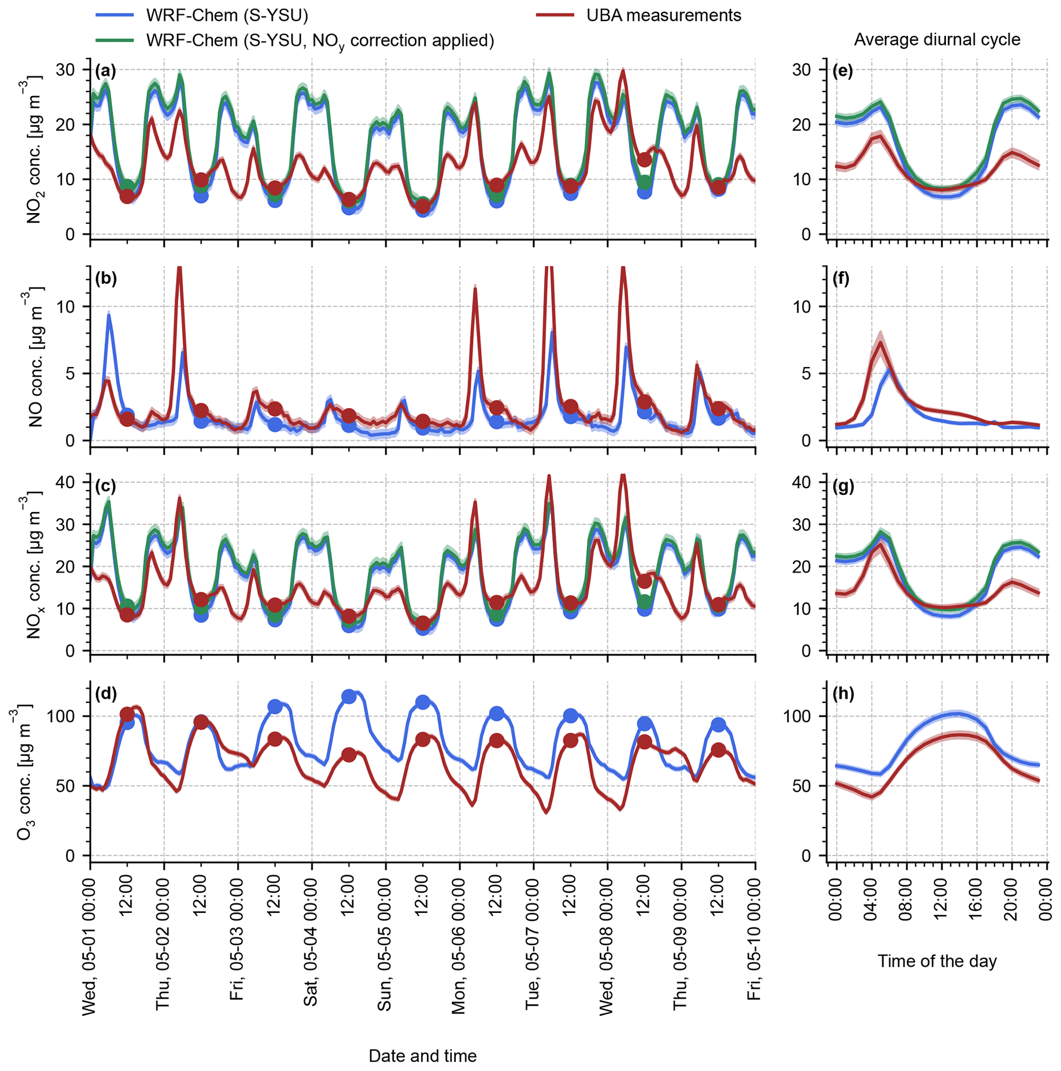
Figure 3 Time series of NO₂, NO, NO_x, and O₃ surface concentrations. The red lines show reference values obtained from the UBA background in situ stations. The blue lines show the simulation results of simulation run S-YSU. Panels (a)–(d) display a time series spanning multiple days (1–10 May 2019), and panels (e)–(h) display the corresponding average concentration values over the entire month of May 2019. Panels (a) and (e) show the diurnal cycle of simulated NO₂ with the NO_y correction factor from Eq. (5) applied in green.

The NO_y correction factor F has a significant impact on the noontime agreement to the observations. Figure 4 depicts the average diurnal cycle of F with a clear correlation to the O₃ surface concentration. This is expected seeing that both O₃ and the cross-sensitive compounds PAN and HNO₃ are produced photochemically. Our results are therefore in good agreement with Poraicu et al. (2023), who obtained a correction factor of ∼ 1.2 at noontime.

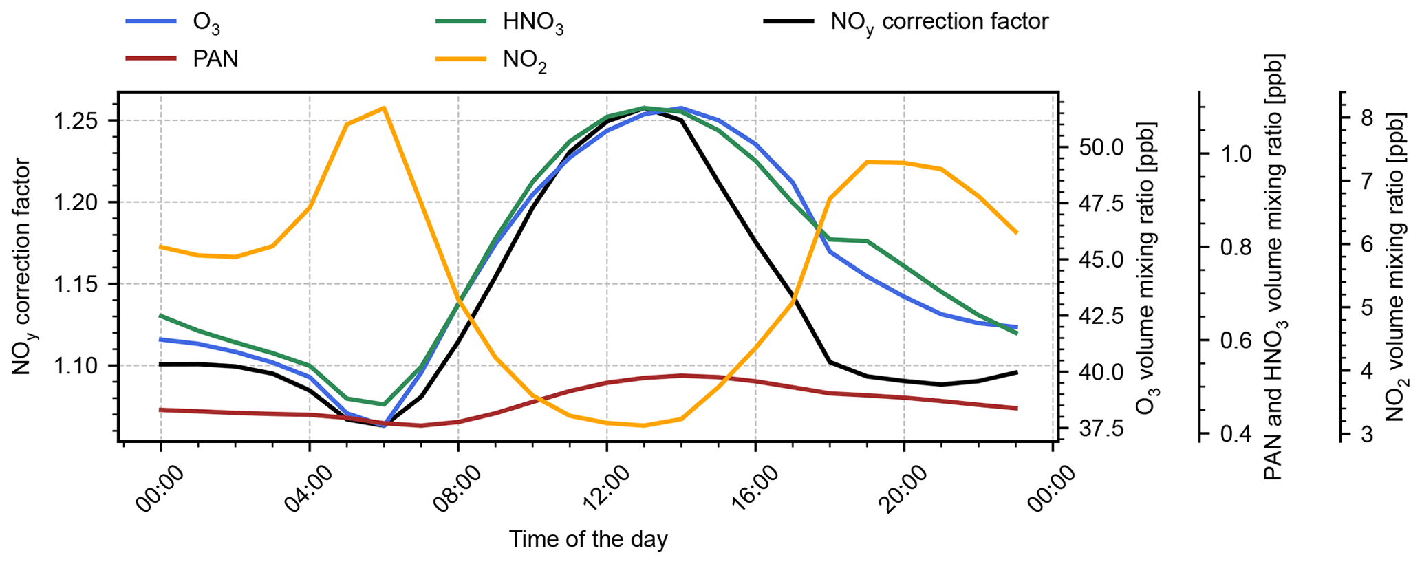
Figure 4 Average diurnal cycle of the NO_y correction factor (black), simulated O₃ (blue), HNO₃ (green), PAN (red), and NO₂ (orange). The simulation results are taken from the base run S-YSU and given as volume mixing ratios in order to conform to Eq. (5).

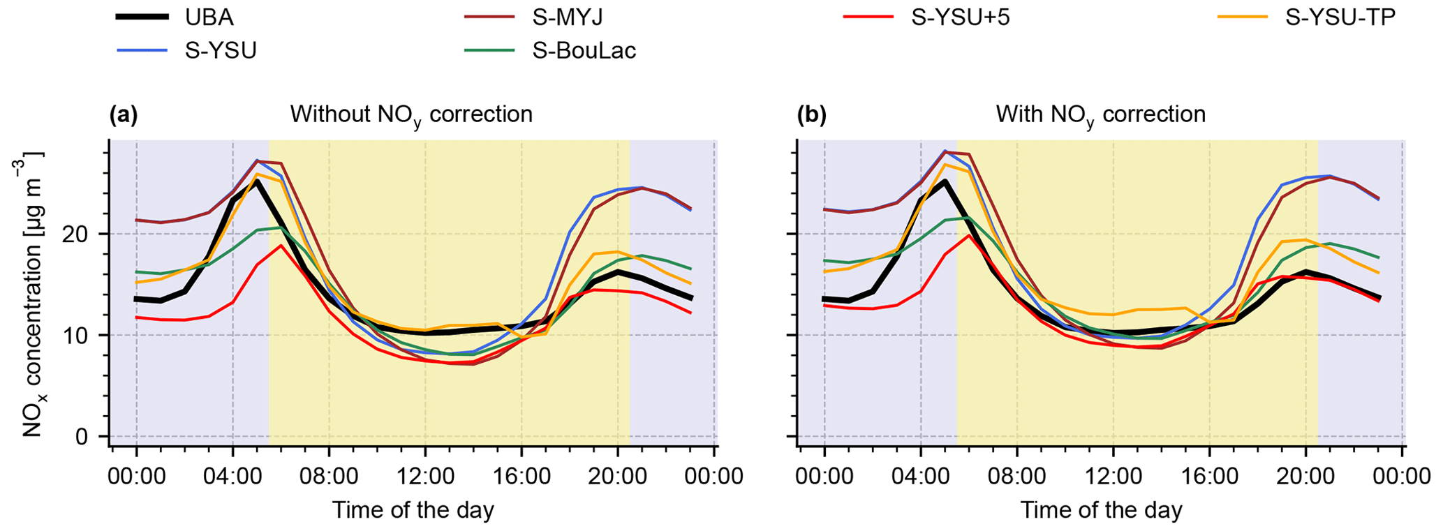
We now compare these baseline results to the results obtained from the alternative model runs, as described in Sect. 2.2, 2.3, and 2.4. Figure 5 shows the diurnal cycle of simulated and observed surface NO₂ for all simulation variants, with and without NO_y correction applied. All model variants, except for S-YSU-TP (the run with tuned temporal emission profiles), show generally better agreement with the noontime observations when the NO_y correction is applied. The diurnal cycle produced by S-MYJ is similar to that of S-YSU, which has been discussed earlier, with the exception of a slightly stronger noontime low bias (−23.9 % without NO_y correction, −4.5 % with NO_y correction). S-BouLac, however, produces noontime values similar to S-YSU with highly reduced bias at night-time (+16.1 % without NO_y correction, +23.8 % with NO_y correction). This motivates us to further investigate how the diurnal cycle of surface NO₂ is influenced by the choice of PBL scheme.

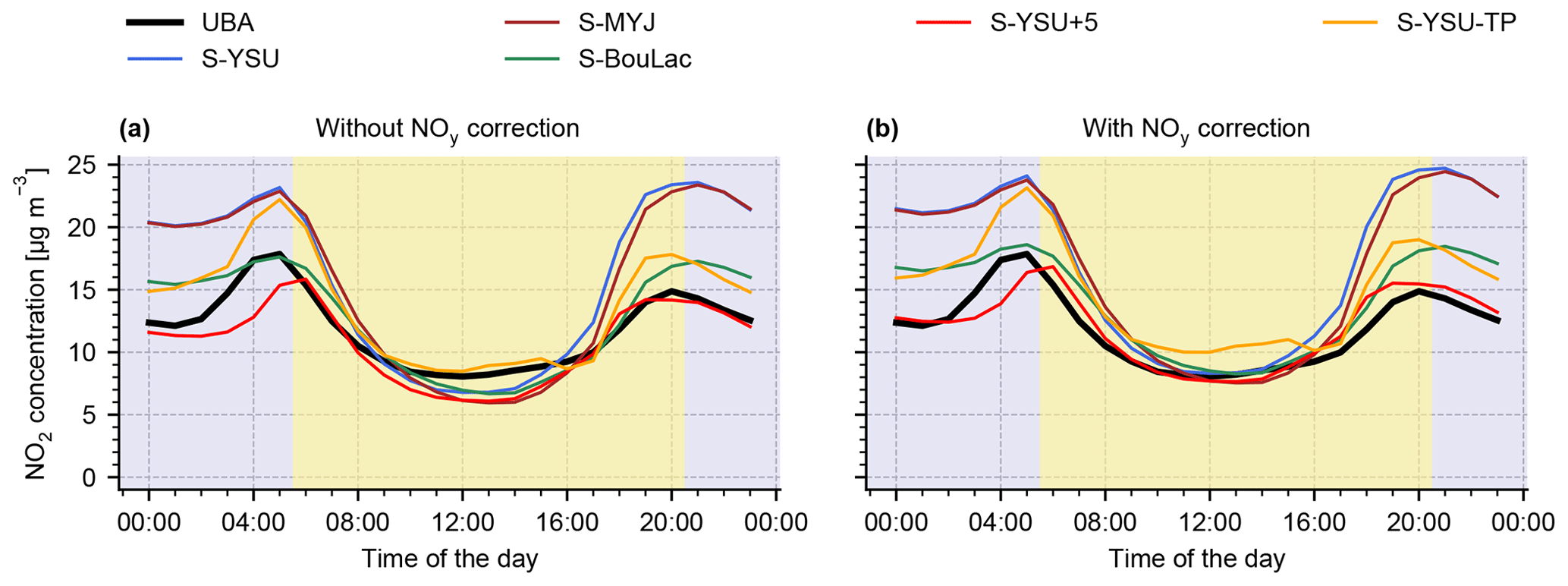
Figure 5 Average diurnal cycles of modelled and observed surface NO₂ at background stations for the different model variants described in Sect. 2.2, 2.3, and 2.4. Daytime and night-time are indicated by yellow and blue background colours, respectively. Panel (a) shows the model results without NO_y correction, while panel (b) shows model results with NO_y correction applied.

Figure 6a shows the diurnal cycle of boundary layer height (BLH) in the YSU, MYJ, and BouLac scheme, averaged over all model cells that contain a UBA station (i.e. the same cells that were used to produce Fig. 5). The highest noontime BLHs are obtained from the BouLac scheme, while MYJ yields the lowest noontime values. Note that at night-time this relationship is inverted. Nonetheless, the simulation run S-BouLac produced much lower night-time surface NO₂ than S-YSU and S-MYJ (see Fig. 5). In a well-mixed boundary layer, one would expect the opposite, seeing that the trace gases inside a more shallow boundary layer are confined into a smaller total volume. An explanation to these results is found by examination of the mixing coefficients k_h in the lowest two model layers, as shown in Fig. 6b: at night-time, all three schemes produce average mixing coefficients smaller than 1 m² s⁻¹ in the lowest layer. As described in Sect. 2.3, the mixing coefficients are clipped to 1 m² s⁻¹ over rural regions and 2 m² s⁻¹ over urban regions, i.e. the average night-time mixing strength is then identical for all three schemes. One layer above, however, the clipping threshold for k_h is exceeded by BouLac and MYJ. As a consequence, the NO_x emissions at the surface are more efficiently diluted by vertical transport; hence, night-time NO₂ concentrations in S-BouLac are significantly lower. The explanation is equally applicable to the daytime observations, for example where S-MYJ shows the lowest surface NO₂ concentrations and the highest mixing coefficients out of all three runs. Figure 7 demonstrates that the mixing coefficients quickly reach far higher values in higher layers during daytime (shown here for the YSU scheme). In that case, clipping the mixing coefficient to 1, 2, or even 5 m² s⁻¹ (as in S-YSU+5) has no effect, as opposed to night-time, when the mixing coefficients are mostly smaller than 1 m² s⁻¹. As a result, the diurnal cycle of surface NO₂ in the simulation run S-YSU+5 (see Fig. 5) shows significantly reduced night-time bias (−11.1 % without NO_y correction, as opposed to +53.1 % in S-YSU, and −3.1 % with NO_y correction, as opposed to −60.5 % in S-YSU) and noontime biases comparable to those of S-YSU and S-MYJ (−23.5 % without NO_y correction and −4.4 % with NO_y correction). S-YSU+5 outperforms all other simulation runs at daytime and night-time. It should be emphasized that this analysis is based on averaged values of the mixing coefficient. Due to the spatial and temporal variability of k_h, individual model cells may be subject to the clipping procedure during daytime as well, explaining the slightly lower noontime NO₂ concentrations observed in S-YSU+5. Figure A2 in Appendix A shows a corresponding histogram of noontime mixing coefficients. Similarly, regions at the top of the PBL are affected by the clipping but play no significant role in our evaluation study.

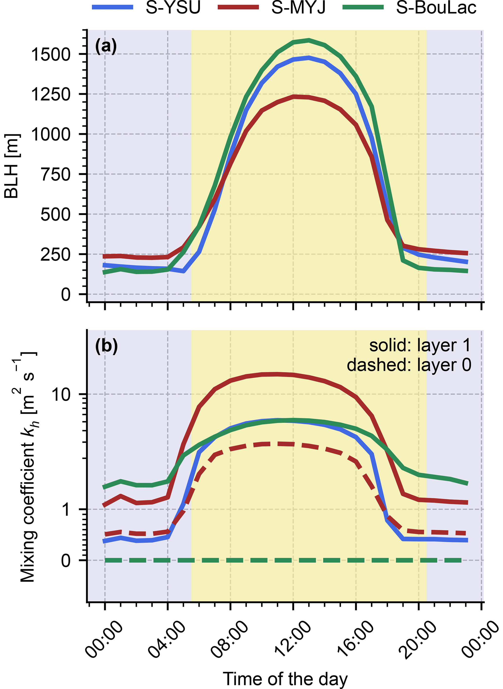
Figure 6 Diurnal cycles of boundary layer height (a) and mixing coefficient k_h (b) averaged over all model cells than contain a UBA station (i.e. the same cells that were used to produce Fig. 5). Note that the y axis in panel (b) has a linear scale from 0 to 1 m² s⁻¹ and a logarithmic scale above. Day- and night-time are indicated by yellow and blue background colours, respectively.

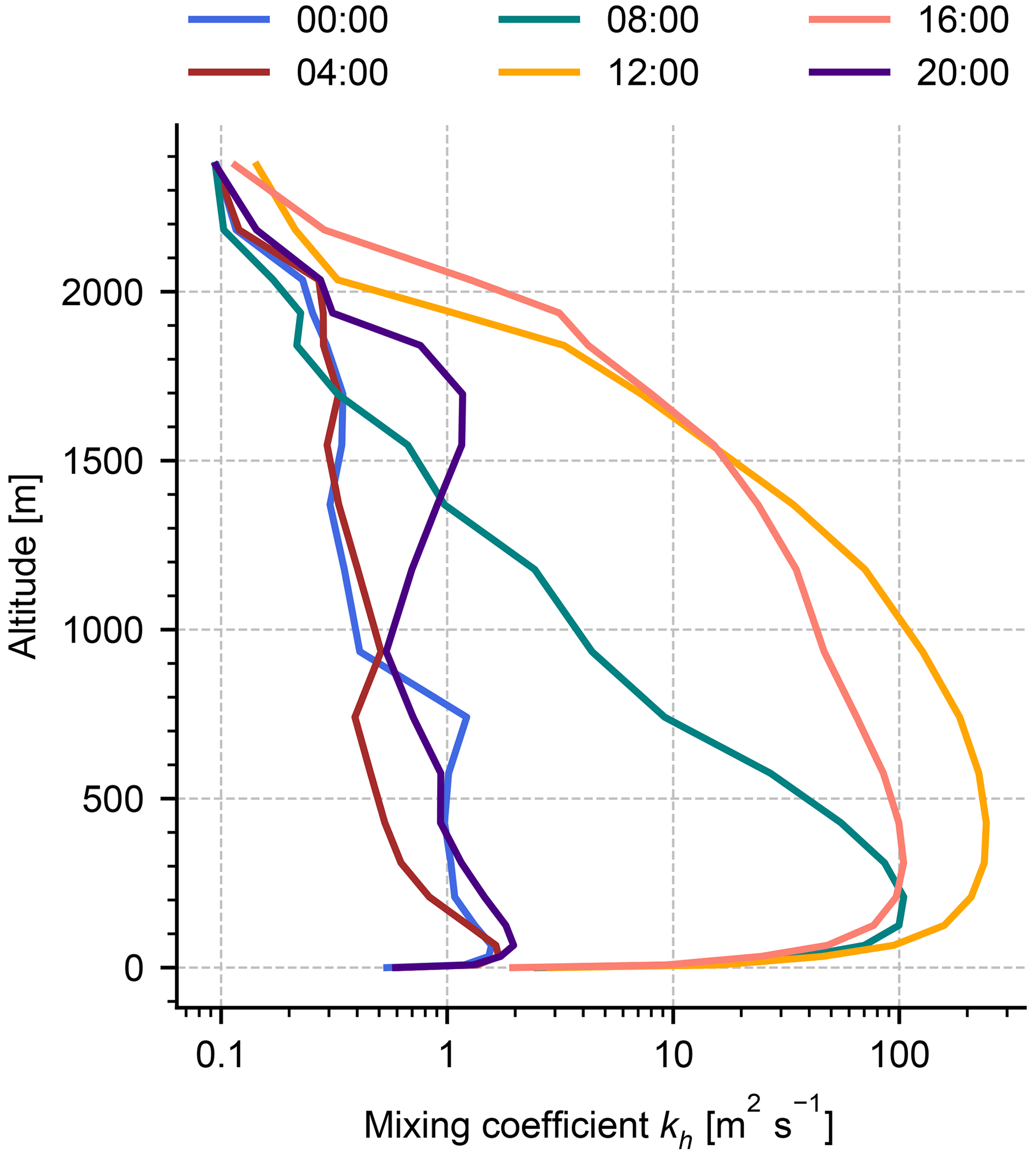
Figure 7 Average mixing coefficient profiles from the YSU PBL scheme at different hours of the day.

Next we discuss the results of the simulation run S-YSU-TP with tuned temporal emission profiles. Figure 5a shows, that without NO_y correction, the corresponding model run S-YSU-TP outperforms S-YSU, S-MYJ, and S-BouLac. The model biases are reduced to +5.2 % and −20.4 % at daytime and night-time respectively. As such, it also outperforms S-YSU+5 at noontime. With NO_y correction applied, S-YSU-TP becomes the worst-performing model run at noontime, with a high model bias of +24.1 %, while still outperforming S-YSU, S-MYJ, and S-BouLac at night-time. Nonetheless, S-YSU-TP is overall outperformed by S-YSU+5. The optimization of temporal profiles alone therefore cannot lead to satisfying results. One way to achieve better model performance in S-YSU-TP would be to scale the total emissions (i.e. through the monthly temporal profiles). This, however, causes severe problems in comparison to the other observational datasets, which indicates that this approach would be inappropriate. Another option would be to run a combined optimization of k_h and the temporal profiles, which could improve the performance of S-YSU+5 further.

So far, the model evaluation was centred around NO₂. Figure 8 shows the comparison of diurnal cycles for NO_x instead. Overall, similar qualitative results are obtained, but there are relevant differences to be discussed. The morning NO peak contributes significantly to the morning NO_x concentration and acts in favour of the original model runs S-YSU and S-MYJ, as well as S-YSU-TP, reducing their overall bias. The peak is caused by photolysis of NO₂ and the night-time reservoir species (such as NO₃ and N₂O₅). The model, however, obtains the high morning concentrations in addition to the chemical production by underestimating vertical mixing (as shown earlier in the comparison between model runs), i.e. for the wrong reason. Based on the mean daytime bias (−3.0 %), S-YSU+5 still outperforms the other runs. At noontime, however, S-YSU+5 shows a slightly larger low bias (−12.1 %) than the other runs, and it is outperformed by S-BouLac and S-YSU-TP during the night-time, with a bias of −16.3 %. The results of Fig. 8 suggest that the modelled NO_x concentrations can be further optimized by slightly reducing the lower mixing threshold starting from a value of 5 m² s⁻¹. However, this would worsen the agreement with the observed NO₂ concentrations from Fig. 5 as well. Another noteworthy observation is the general overestimation of ${\mathrm{NO}}_{\mathrm{2}}/\mathrm{NO}$ ratios throughout the day (see Fig. 3), which was observed across all model runs. It was tested in further control runs (not shown here), that scaling of O₃ boundary conditions and VOC emissions barely impacts the ${\mathrm{NO}}_{\mathrm{2}}/\mathrm{NO}$ ratio of the model. Therefore, it is unlikely that the overestimation of ${\mathrm{NO}}_{\mathrm{2}}/\mathrm{NO}$ ratios relates to NO oxygenation alone. Instead, more complex processes in the night-time NO_x chemistry (see, e.g. Knote et al., 2015) or the lack of daytime HONO chemistry could be possible causes. Finally, ${\mathrm{NO}}_{\mathrm{2}}/\mathrm{NO}$ ratios could be influenced by the choice of NO_x speciation profiles. In this study, we have used a uniform speciation based on literature values, but it can be assumed that in reality speciation differs between individual emission sectors (see, e.g. Wild et al., 2017; Jimenez et al., 2000; Richmond-Bryant et al., 2017; Costantini et al., 2016).

Figure 8 Like Fig. 5 but for NO_x instead of NO₂.

The results of this section are summarized in Tables 3 and 4, where only NO_y-corrected results are shown.

Table 3 Statistical summary of the performance of the five model runs at noontime (12:00 LT), daytime (06:00–20:00 LT), and night-time (21:00–05:00 LT). All numbers refer to simulated NO₂ at the location of the background UBA stations.

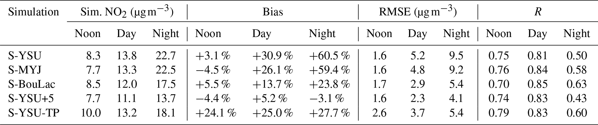
Observed mean at noontime: 8.1 µg m⁻³. Observed mean at daytime: 10.5 µg m⁻³. Observed mean at night-time: 14.1 µg m⁻³.

Table 4 Statistical summary of the performance of the five model runs at noontime (12:00 LT), daytime (06:00–20:00 LT), and night-time (21:00–05:00 LT). All numbers refer to simulated NO_x at the location of the background UBA stations.

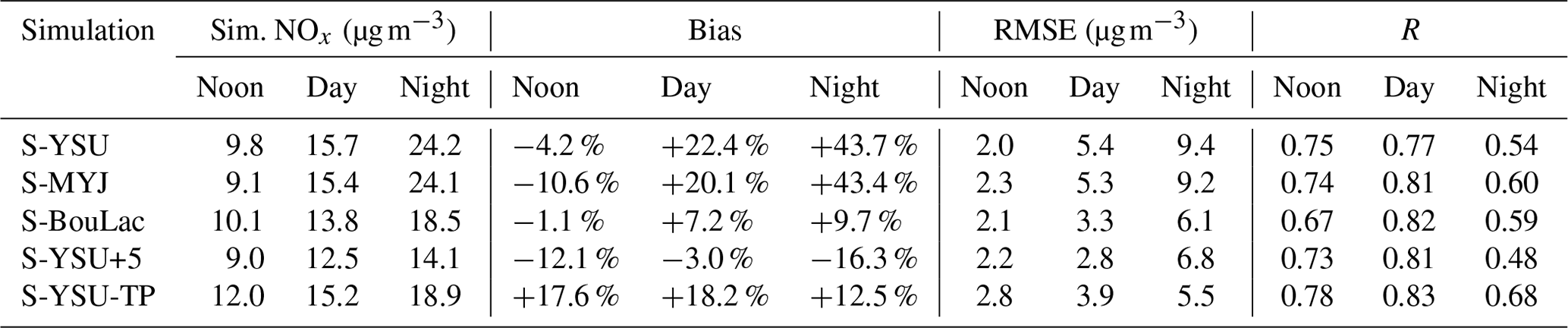
Observed mean at noontime: 10.2 µg m⁻³. Observed mean at daytime: 12.9 µg m⁻³. Observed mean at night-time: 16.8 µg m⁻³.

3.2 Comparison of NO₂ vertical column densities

As a second diagnostic, we compare simulated NO₂ VCDs to observations of the TROPOMI satellite instrument (see Veefkind et al., 2012). The satellite overpass occurs daily, typically at 13:30 LT in central Europe, with a pixel size of 3.5 km × 5.5 km in nadir-viewing geometry. TROPOMI measures spectra of backscattered sunlight from Earth's surface, from which tropospheric slant column densities (SCDs) are computed using differential optical absorption spectroscopy (DOAS; see Platt and Stutz, 2008). Tropospheric VCDs are obtained from tropospheric SCDs via

$$\begin{array}{}\text{(6)}& {\text{VCD}}_{\mathrm{trop}}={\displaystyle \frac{{\text{SCD}}_{\mathrm{trop}}}{{\text{AMF}}_{\mathrm{trop}}}},\end{array}$$

where AMF_trop stands for the tropospheric air mass factor. The tropospheric AMF depends on a number of atmospheric and surface conditions and assumptions, e.g. cloud properties, the stratospheric column, surface albedo, and the a priori NO₂ profile. In the TROPOMI retrieval, the NO₂ a priori profiles are taken from the TM5 global CT model (see Krol et al., 2005; Williams et al., 2017), with a spatial resolution of ∼ 1^∘ × 1^∘ ≈ 110 km × 70 km where our simulation domain D2 is located. A detailed description of the retrieval algorithm can be found in van Geffen et al. (2022).

Simulated VCDs are obtained by vertical integration of box VCDs (partial columns) from WRF-Chem. The WRF-Chem output is interpolated to the vertical grid of the TM5 model. The box VCDs are computed by multiplying the NO₂ concentration within each model grid cell with its vertical extent. The partial columns are then summed up:

$$\begin{array}{}\text{(7)}& {\text{VCD}}_{\mathrm{sim}}=\sum _{l<l_{\mathrm{tp}}}{c}_l\cdot \mathrm{\Delta }{h}_l,\end{array}$$

where VCD_sim denotes the simulated VCD, l the TM5 model layer index, l_tp the tropopause layer index, c_l the NO₂ concentration in layer l, and Δh_l the vertical extent of layer l. Following this, pairs of simulated and observed VCDs are obtained by interpolating the WRF-Chem data to the horizontal TROPOMI grid in space and time.

In order to make a representative comparison between simulated and observed VCDs, the following further aspects are taken into consideration.

• 1.

  TROPOMI is not equally sensitive to all layers of the troposphere. This circumstance is described by the averaging kernels (AKs; see van Geffen et al., 2022). Furthermore, the AMF depends on the NO₂ a priori profiles provided by the TM5 model. It has been demonstrated that replacing TM5 a priori profiles with profiles from high-resolution RCT models improves the VCD retrieval significantly (see, e.g. Ialongo et al., 2020; Tack et al., 2021; Liu et al., 2021).

  We incorporate the AKs and our simulated high-resolution NO₂ a priori profiles by computing corrected observed VCDs following Eskes et al. (2019):

  $$\begin{array}{}\text{(8)}& \begin{array}{rl}{\text{VCD}}_{\mathrm{obs},\mathrm{corr}}& ={\text{VCD}}_{\mathrm{obs}}\cdot {\displaystyle \frac{{\text{AMF}}_{\mathrm{trop}}}{\text{AMF}}}\\ & \cdot {\displaystyle \frac{{\sum }_{l<l_{\mathrm{tp}}}{c}_l\cdot \mathrm{\Delta }{h}_l}{{\sum }_{l<l_{\mathrm{tp}}}{c}_l\cdot \mathrm{\Delta }{h}_l\cdot A_l}},\end{array}\end{array}$$

  where VCD_obs denotes the observed NO₂ VCD, AMF_trop the tropospheric AMF, and A the averaging kernel vector.

• 2.

  Each observed VCD has an associated “QA value” that describes the retrieval quality on a range from 0 (bad) to 1 (good) (see van Geffen et al., 2022). QA values of ≥0.75 also require the cloud radiance fraction (CRF) to be smaller than 0.5, which effectively acts as a cloud filter. The effect of clouds on the measurement process depends on the height of the cloud layer: high clouds can shield off lower layers of the atmosphere, decreasing the NO₂ sensitivity to almost zero below the cloud layer. In contrast, cloud layers directly below NO₂ layers can enhance the observed NO₂ absorption due to the increased cloud albedo. If cloud layers and NO₂ layers are at the same altitude, NO₂ absorption can be increased by an enhanced light path due to multiple scattering. The influence of clouds on satellite measurements of NO₂ has been discussed, e.g. in Martin et al. (2002), Kokhanovsky and Rozanov (2008), and Liu et al. (2021). We apply a QA filter that removes all observations with QA <0.75, as recommended by Eskes et al. (2019).

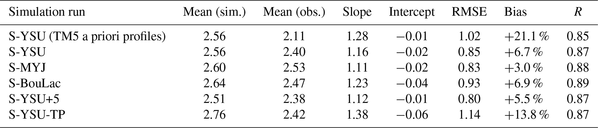
Figure 9 shows the result of our comparison in the form of monthly mean values (i.e. the total average over May 2019) for the base simulation run S-YSU. Figure 9a–e show the comparison between simulated NO₂ VCDs and TROPOMI observations using the TM5 NO₂ a priori profiles. Strong enhancements occur in western Germany (Ruhr region) and along the Rhine River. Moderate enhancements occur over logistical hotspots (e.g. the port of Hamburg with a nearby coal power plant), and larger cities (e.g. Berlin and Munich; see Fig. 11 for an overview of the geographical regions mentioned here). Figure 9c shows the difference between simulated and observed VCDs and reveals the model's tendency to overestimate the observed VCDs. The overestimation is close to zero in rural regions but reaches up to 10¹⁶ molec. cm⁻² over hotspot regions. The simulated and observed VCDs correlate with an R value of 0.85, an RMSE of 1.02×10¹⁵ molec. cm⁻², and a bias of +21.1 %. A linear fit through the point cloud (Fig 9e) yields a slope of 1.28 and an intercept of $-\mathrm{0.01}\times {\mathrm{10}}^{\mathrm{15}}$ molec. cm⁻². Figure 9f–j show the same comparison but with recomputed air mass factors according to Eq. (8). The comparison improves, with an R value of 0.87, an RMSE of 0.85×10¹⁵ molec. cm⁻², a bias of +6.7 %, a slope of 1.16, and an intercept of $-\mathrm{0.02}\times {\mathrm{10}}^{\mathrm{15}}$ molec. cm⁻².

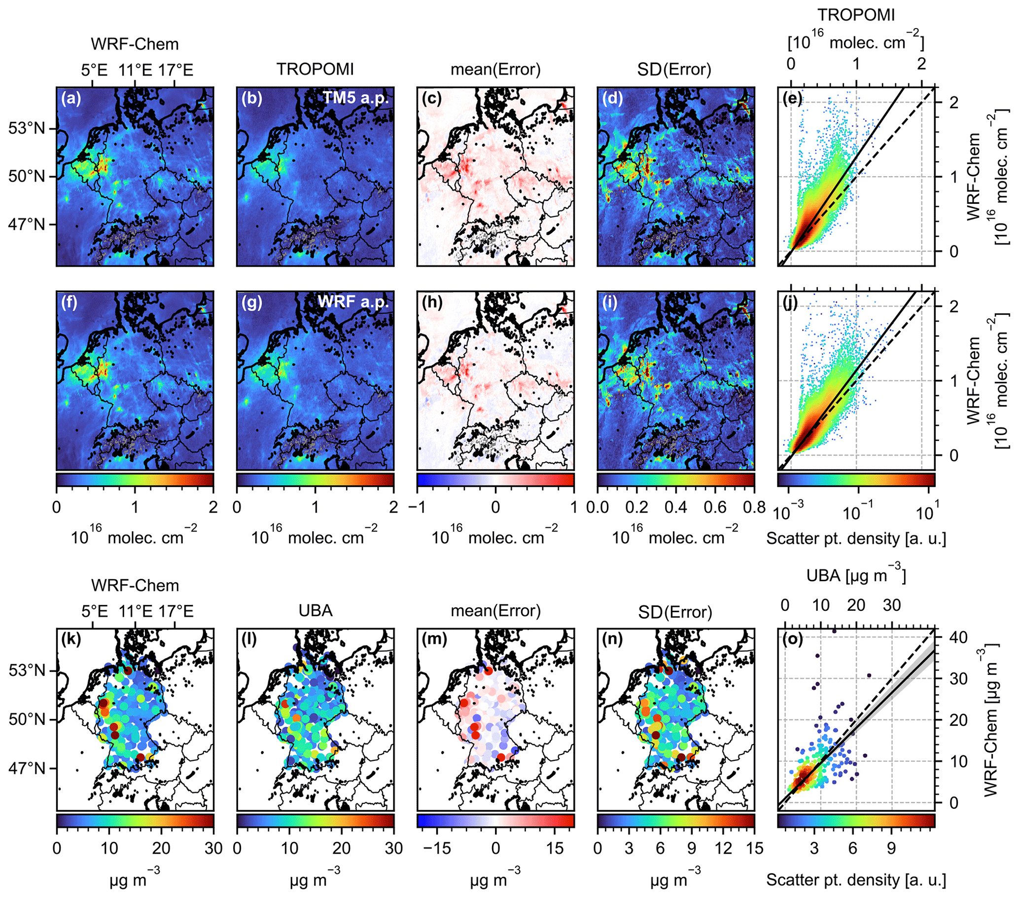
Figure 9 Comparison of simulated and observed NO₂ VCDs (a)–(j) and surface NO₂ concentrations (k)–(o) for the base model run S-YSU. The first row (a)–(e) shows the comparison to the original observations using low-resolution TM5 a priori NO₂ profiles. The second row (f)–(j) shows the comparison with reprocessed observations using high-resolution WRF-Chem a priori profiles and averaging kernels. All satellite observations were restricted to cases with QA ≥0.75. The third row (k)–(o) shows a comparison between simulated and observed surface NO₂ concentrations from “background” stations.

Figure 9k–o show the spatial distribution of simulated and observed surface NO₂ concentrations from the UBA background stations. Model overestimations of NO₂ VCD and surface concentration occur in similar geographic regions, particularly in the Ruhr region, along the Rhine river, and the port of Hamburg. This hints towards a possible overestimation of NO_x emissions in these regions. Figure 10 presents further comparisons of simulated and observed NO₂ VCDs for different simulation runs. Here, we only show comparisons using reprocessed observations according to Eq. (8). Table 5 summarizes the results of this section. The main observation to be made here is that the high sensitivity of the simulated surface concentrations (see Sect. 3.1) to the PBL scheme and vertical mixing strength is not found in the comparison for column densities, as expected for a trace gas column. Even the base run S-YSU shows good results, with a slope of 1.16 and an RMSE of 0.85×10¹⁵ molec. cm⁻². S-YSU+5 achieves the lowest RMSE (0.80×10¹⁵ molec. cm⁻²) and slightly better slope of 1.12. In addition, the overestimation over western Germany appears to be reduced compared to all other runs. Overall, S-YSU, S-MYJ, S-BouLac, and S-YSU+5 perform quite similarly with respect to the statistical diagnostics shown here (with the exception of S-BouLac, showing a significantly higher RMSE of 0.93×10¹⁵ molec. cm⁻²). This is expected, seeing that in the first order the tropospheric column is a measure of total NO₂, which may vary only slightly across these simulation runs. S-YSU-TP shows significantly larger simulated VCDs, resulting in a bias of +13.8 % and an RMSE of 1.14×10¹⁵ molec. cm⁻² (the worst out of all runs). Figure 10r shows that S-YSU-TP overestimates the NO₂ VCDs over western Germany, the Netherlands, and Belgium more strongly than the other runs, while not performing noticeably better in any other part of the domain. The combined results of Tables 3, 4, and 5 favour S-YSU+5, the run with enhanced vertical mixing, as the best setup.

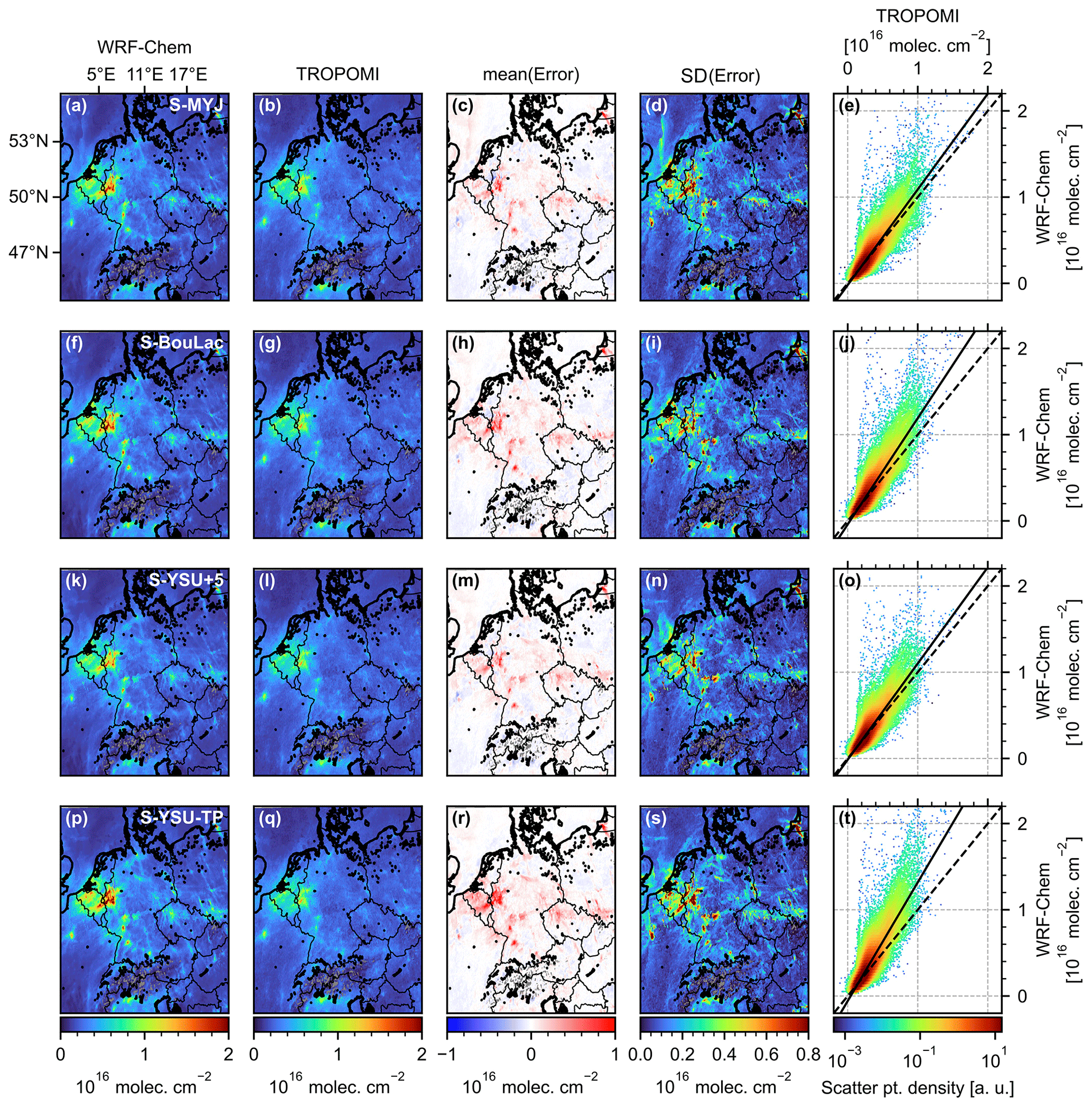
Figure 10 Further comparisons of simulated and observed NO₂ VCDs for the remaining simulation runs S-MYJ, S-BouLac, S-YSU+5, and S-YSU-TP. The comparison for each model run is in direct analogy to Fig. 9f–j.

Table 5 Statistical summary of the results shown in Figs. 9 and 10.

Means and RMSE are given in units of 10¹⁵ molec. cm⁻².

3.3 Comparison of NO₂ concentration profiles

As a third diagnostic we compare modelled NO₂ concentration profiles to profiles obtained from MAX-DOAS (multi-axis differential optical absorption spectroscopy) measurements. In contrast to the data shown in Sect. 3.1 and 3.2, profile comparison allows for assessment of the model's capability to capture vertical distributions of NO₂. MAX-DOAS measurements use the DOAS principle (see Platt and Stutz, 2008) to obtain trace gas differential slant column densities (dSCDs) at different elevation angles. By application of an inversion algorithm a discretized concentration vector c is obtained, whose entries denote the target gas concentration in different atmospheric layers. An overview of different inversion algorithms can be found in Frieß et al. (2019). We use data from the FRM4DOAS network (see Fayt et al., 2021), which applies the Mexican MAX-DOAS fit (MMF; see Friedrich et al., 2019) and the Mainz Profile Algorithm (MAPA; see Beirle et al., 2019). While MMF is based on optimal estimation (see Rodgers, 2000), MAPA uses Monte Carlo simulation in order to determine profile shape parameters which combine (possibly lifted) box profiles and exponential profiles. Purely exponential concentration profiles, however, cannot be obtained from the current version of MAPA.

Five MAX-DOAS instruments are operated within our simulation domain D2: Mainz (Germany), Bremen (Germany), Heidelberg (Germany), De Bilt (Netherlands), and Uccle (Belgium). Figure 11 shows the locations of these stations. A single station typically yields 2–4 NO₂ profile measurements per hour. In order to compare simulated and observed profiles, the WRF-Chem dataset is interpolated to the geolocations and measurement times of the MAX-DOAS instruments. The uncertainty of the simulated NO₂ profiles is obtained as the standard deviation of the surrounding eight WRF-Chem grid cells.

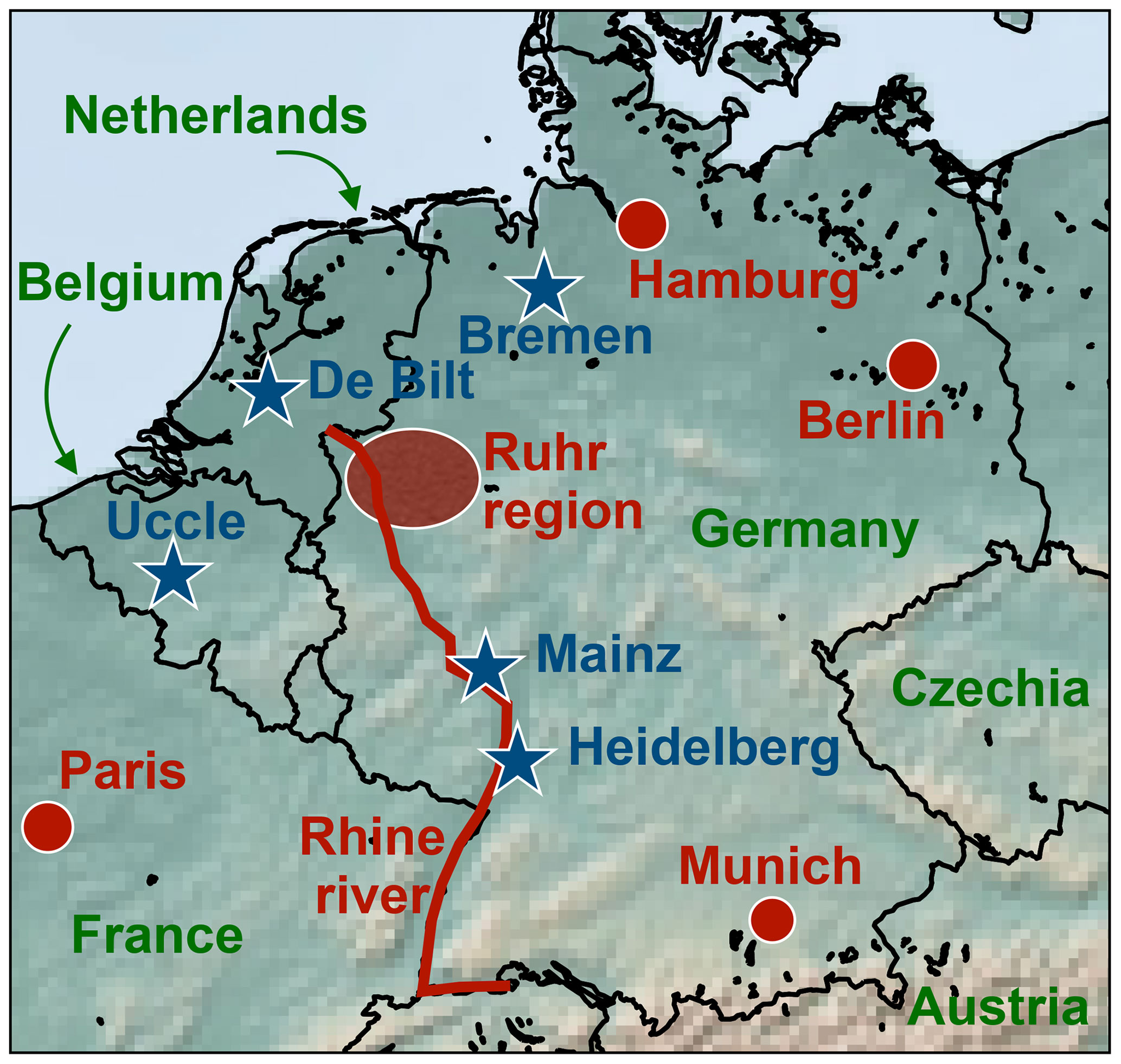
Figure 11 Part of central Europe covering Germany, Belgium, and the Netherlands with important geographical regions marked in red. The blue stars show the locations of the MAX-DOAS measurements shown in Sect. 3.3.

The MMF inversion algorithm provides averaging kernels (AKs), represented by a (h×h) matrix, where h is the number of atmospheric layers considered. Here, h=20, comprising retrieval altitudes up to 4 km. Using the AKs, the MAX-DOAS measuring sensitivity to different altitudes can be applied to the simulated profiles. For this purpose the simulated NO₂ profiles are vertically interpolated to the layers of the MAX-DOAS retrieval grid. Following this, the AKs are applied via

$$\begin{array}{}\text{(9)}& {\mathit{c}}_{\mathrm{sim},\mathrm{corr}}=\mathbf{A}{\mathit{c}}_{\mathrm{sim}}+\left(\textcolor{red}{}-\mathbf{A}\right){\mathit{c}}_{\mathrm{ap}},\end{array}$$

where c_sim, corr is the corrected simulated profile, A the averaging kernel matrix, c_sim the original simulated profile, the unity matrix, and c_ap the a priori profile (see Rodgers and Connor, 2003). MAPA neither provides AKs nor depends on an a priori profile. All profiles flagged as “erroneous” by MAPA were dismissed from the evaluation.

Figure 12 shows averaged NO₂ profiles from the MAX-DOAS station Mainz, Germany, in the time window from 11:00 to 14:00 LT for a selection of individual days, as well as the corresponding modelled profiles from the base run S-YSU. The aim is to give an overview of the variety of observed and modelled profile shapes. Additionally, the average NO₂ surface concentrations measured by UBA stations within a radius of 5 km of the MAX-DOAS instrument are drawn as coloured scatter markers at 0 m altitude.

Figure 12 Comparison of average NO₂ profiles for Mainz around noontime (11:00–14:00 LT) for 4 exemplary days: (a) 3 May 2019, (b) 17 May 2019, (c) 1 May 2019, and (d) 27 May 2019. Additionally, average NO₂ surface concentrations measured by UBA stations within a radius of 5 km of the MAX-DOAS instrument are drawn as coloured scatter markers at 0 m altitude. The WRF-Chem results are taken from the base run S-YSU.

Figure 12a shows a typical scenario: on this day (3 May 2019) observation and simulation show comparably good agreement. All three datasets (MMF, MAPA, and WRF-Chem) yield profiles of similar shape. Above an altitude of ∼ 2 km the profiles quickly approach zero, which is characteristic for the transitioning regime between the PBL and the free troposphere. At low altitudes of 0–150 m the simulated profile has a strong exponential tail, typical of the surface layer into which most NO_x emissions are injected (the lowest ∼ 30 m). Furthermore, the simulated profiles show good agreement with the measurements of the nearby UBA in situ stations. High vertical resolution turns out to be crucial for the comparison to surface observations. In the FRM4DOAS dataset, MAPA and MMF were operated with a vertical resolution of 200 m. In a direct comparison, the concentrations obtained from MAPA or MMF in the lowest layer (0–200 m) underestimate the in situ observations at the surface because of the limited vertical resolution of the MAX-DOAS measurements and the rather coarse retrieval grid used by FRM4DOAS. Meanwhile, the lowest layer of our WRF-Chem simulation only spans 0–8 m, which allows for a much more representative comparison.

Figure 12b shows a day on which an elevated NO₂ layer was detected by MMF. This is characterized by strongly enhanced NO₂ concentrations at higher altitudes (here at ∼ 500 m). Elevated layers are typically caused by elevated emissions, e.g. from a power plant stack at a few hundred metres in height. Additionally, transport events that advect NO₂ from the surface layer could be the cause. However, no corresponding enhancements can be seen in the simulated NO₂ profile. As described in Sect. 2.1, we do not use vertical emission profiles in the WRF-Chem simulation. Furthermore, it is possible that the overall spatial resolution of our simulation limits its ability to model comparable elevated trace gas abundances. With a resolution of 3 km × 3 km × 100 m at ∼ 500 m altitude, trace gas concentrations are diluted into comparably large grid cell volumes. Lastly, horizontal concentration gradients can be expected near strong emission sources. These can lead to apparently elevated profiles because the MAX-DOAS profile inversion makes the simplifying assumption of horizontally homogeneous distributions. Comparison of simulated and observed elevated layers is therefore an advanced problem and not further addressed here.

Figure 12c shows a day on which the agreement between model and observations was poor, with deviations of >100 %. Such days are outliers and do not represent the overall quality of the model or the measurements; however, they should not remain unmentioned. Possible reasons for such deviations include, e.g. falsely modelled wind directions (affecting trace gas transport) or cloud cover (affecting photolysis).

Figure 12d shows a day on which the modelled profile has an extremely steep exponential gradient in combination with a relatively thin boundary layer. At the transition from the boundary layer to the surface layer (∼ 30–50 m above ground), the simulated profiles show an increase of almost 400 %. Interestingly, on this day (27 May 2019), one of the background stations (DERP009) measured more than twice the surface concentration compared to a nearby traffic station (DERP011). This phenomenon was observed on only one other day (10 May 2019) of the simulated month, on which very similar profile shapes were observed. Furthermore, no MAPA profile is available on this day due to the filtering by error flags. There is also good agreement between modelled and observed profiles above the surface layer. It is therefore plausible to assume that the steep NO₂ gradient towards the surface is not due to a faulty model but, on the contrary, indicates the model's ability to capture scenarios in which, e.g. vertical mixing is mostly suppressed and large portions of the emitted NO₂ remain in the surface layer.

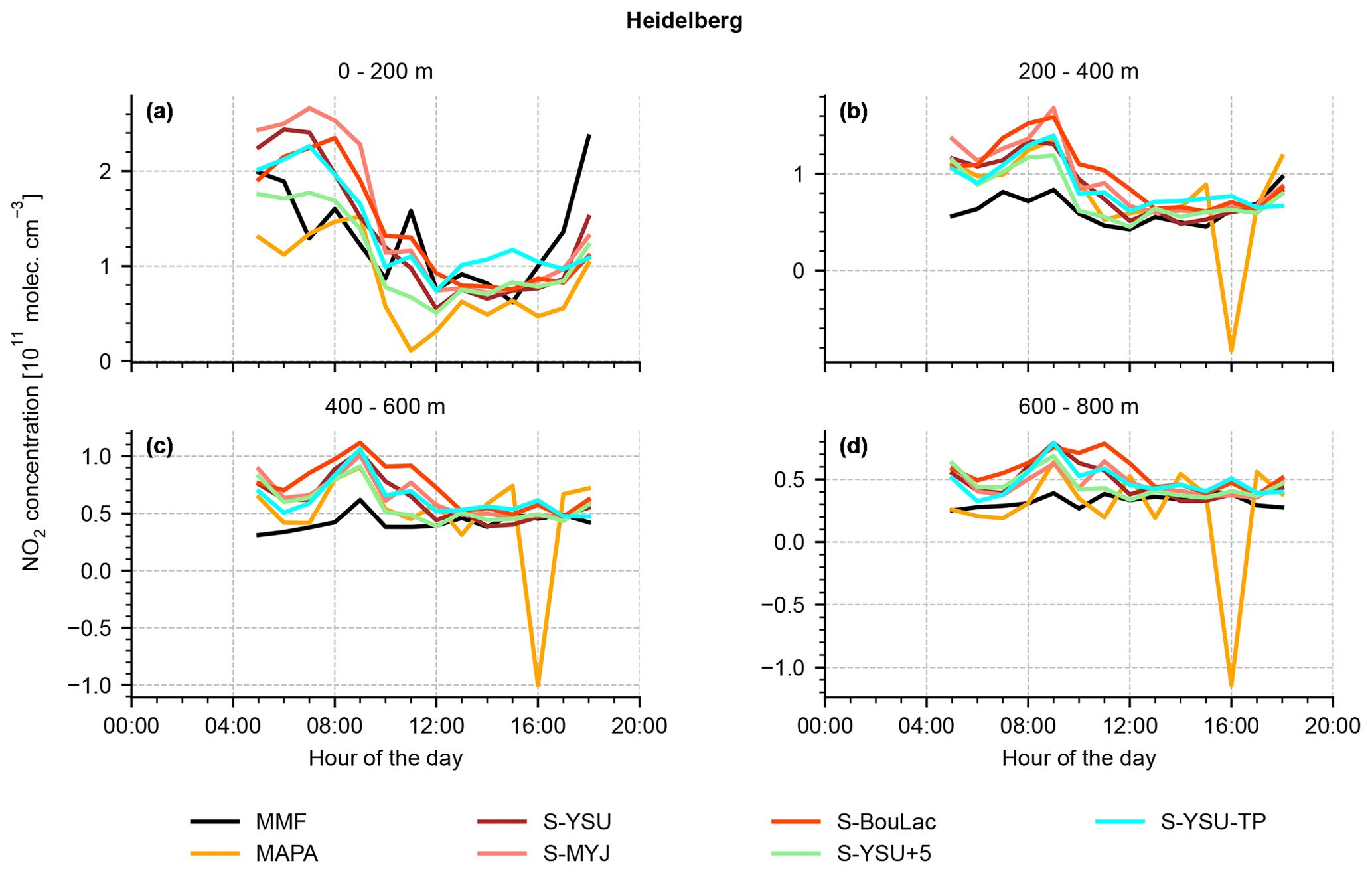
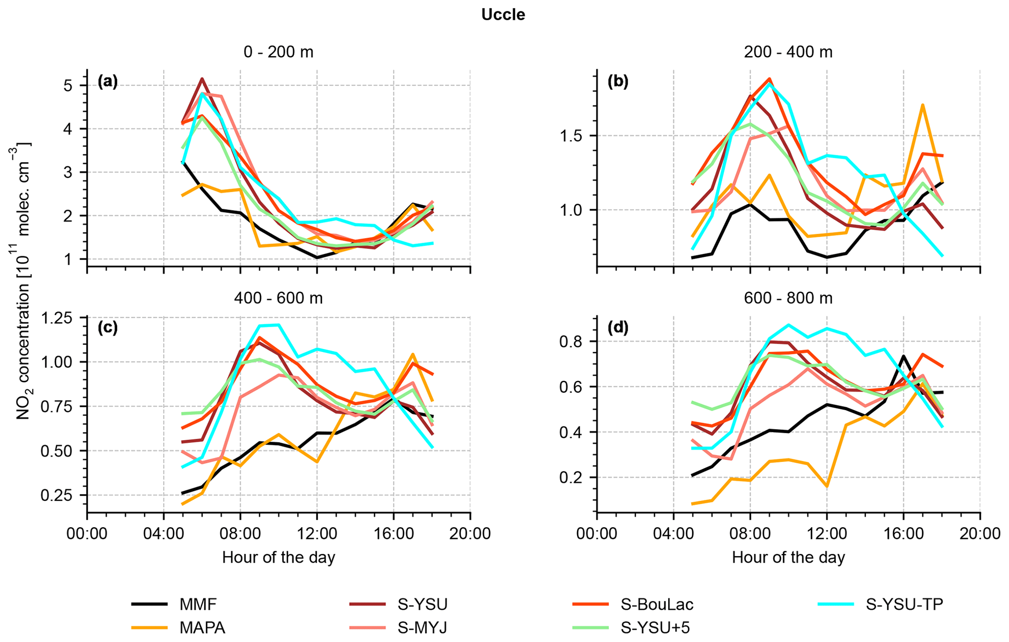
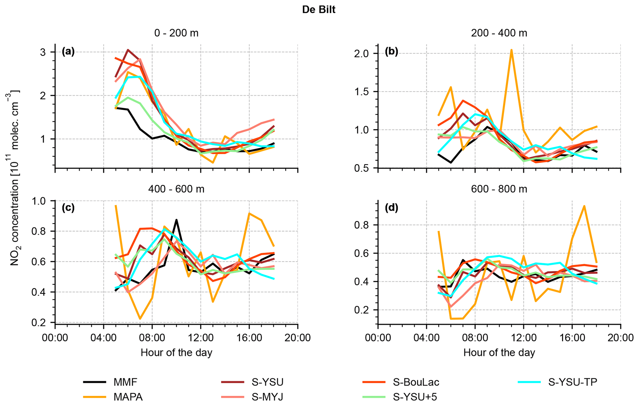
In order to condense the remaining evaluation, we will focus on monthly noontime averages from hereon, i.e. plots of the same structure as shown in Fig. 12 but averaged over the entire simulation period of May 2019 (Figs. 13 and 14). In both figures the right column shows scatter plots of averaged NO₂ concentrations (WRF-Chem vs. MMF, due to availability of AKs) at different altitudes.

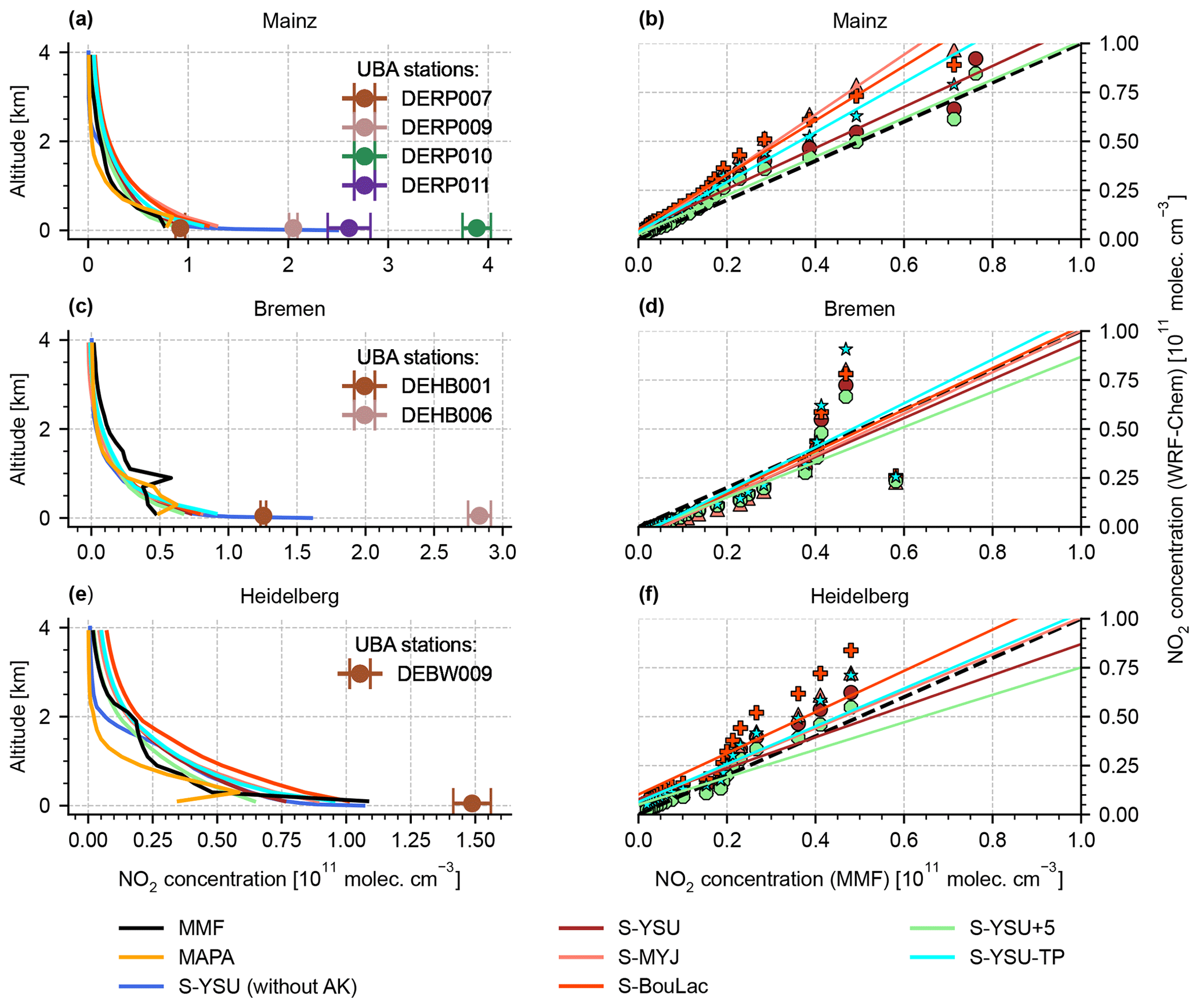
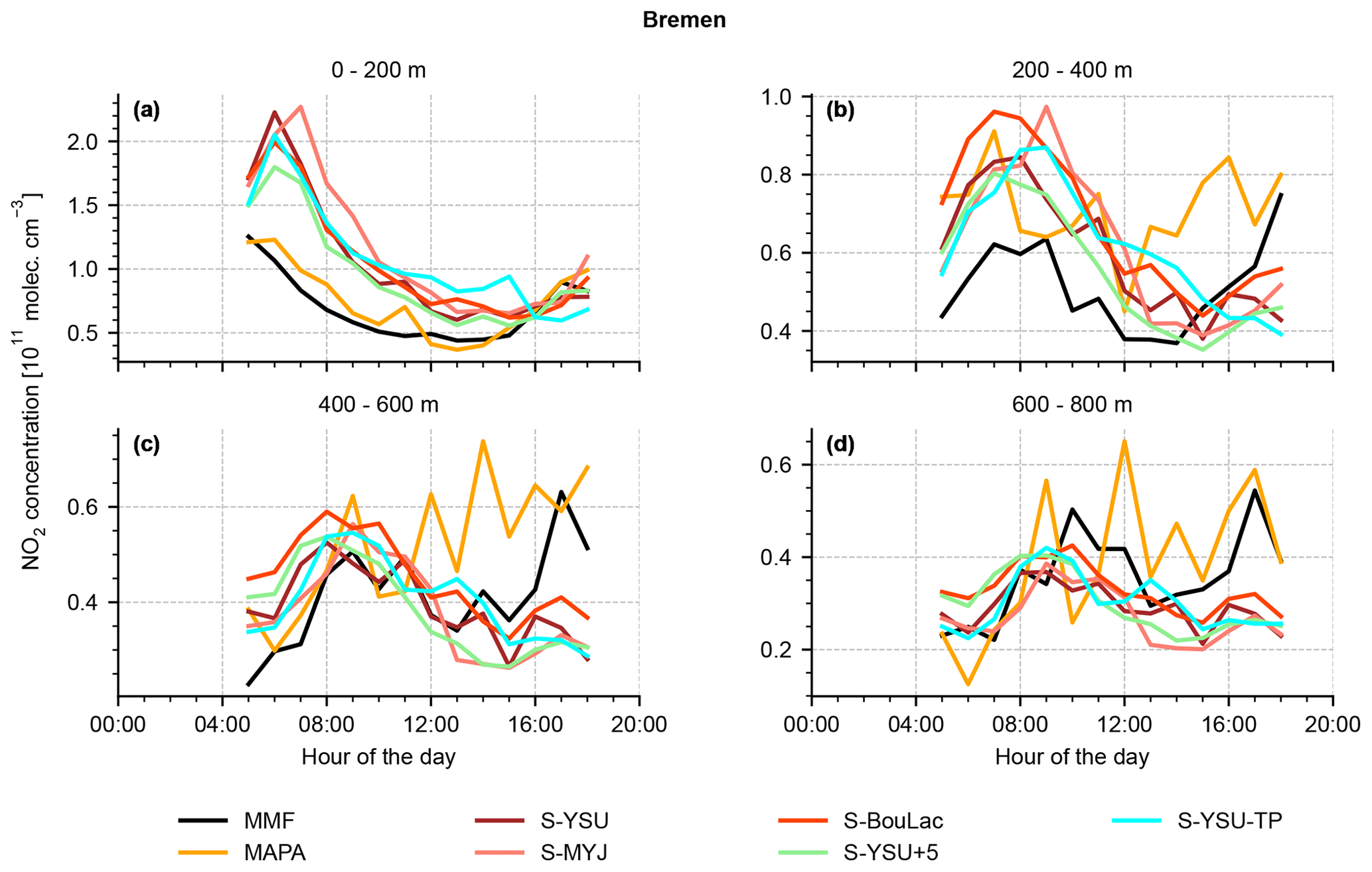
Figure 13 Comparison of averaged NO₂ profiles for Mainz, Bremen, and Heidelberg around noontime (11:00–14:00 LT). The left column (a), (c), (e) shows the NO₂ profiles as obtained by MMF, MAPA, and WRF-Chem. The right column (b), (d), (f) shows the corresponding scatter plots of averaged NO₂ concentrations at different altitudes (here WRF-Chem vs. MMF).

Figure 14 Like Fig. 13 but for the stations De Bilt and Uccle.

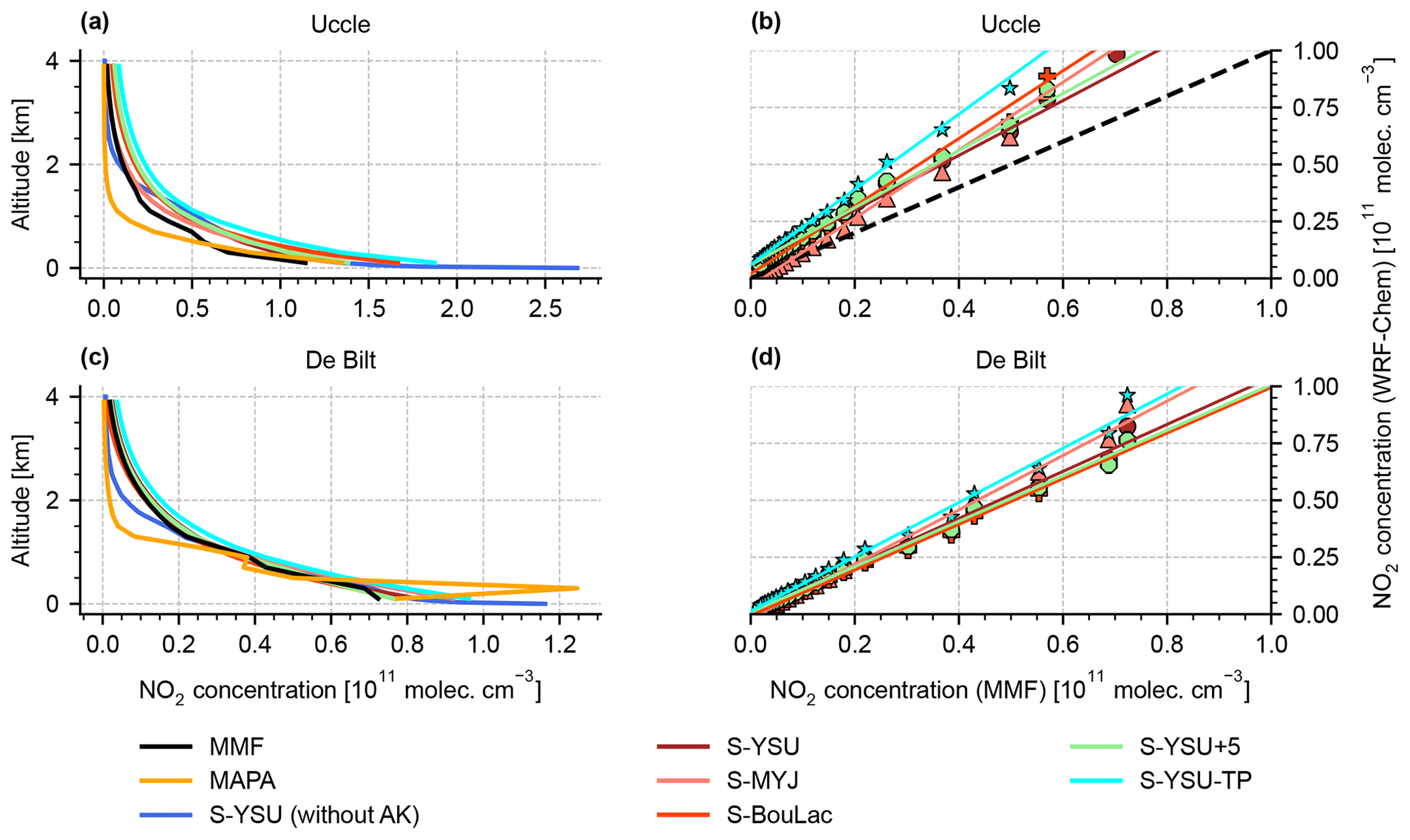
Figure 13 shows the results of the three German MAX-DOAS locations Mainz, Bremen, and Heidelberg. Overall, the three stations show qualitatively similar profiles. At Bremen (see Fig. 13c–d), a consistent elevated layer at ∼ 1000 m altitude was detected, which could be explained by multiple power plants in the vicinity of the instrument. This has been discussed in detail by Bösch (2018). The scatter plots (Fig. 13b, d, f) show a strong correlation between simulation and measurements. A quantitative summary of the comparison is found in Table 6. Although the performance of WRF-Chem varies between the five simulation runs, none of them clearly outperforms the others: the simulation run S-YSU+5, which performed best in Sect. 3.1 and 3.2, outperforms the other runs in four out of five station with respect to RMSE (the exception being Uccle, where S-BouLac has a lower RMSE). However, when considering the bias, S-YSU+5 is outperformed in multiple cases. The simulation run with tuned temporal emission profiles S-YSU-TP produces larger average NO₂ profiles than the base run S-YSU. This effect is especially strong in Uccle and De Bilt and is expected due to the strong shift in emissions towards noontime. However, in Mainz and Heidelberg, S-BouLac (and to some extent, S-MYJ) produce even larger NO₂ concentrations near the ground, which contradicts the general tendencies observed in Sect. 3.1 (see Fig. 5). It should be considered that two exemplary observations of this phenomenon are not significant compared to the hundreds of in situ measurement stations shown in Sect. 3.1. Also, the MAX-DOAS stations are closer to strong emission sources in generally more polluted locations, whereas only background stations were considered in the comparison to in situ observations. A temporally resolved version of the comparison is found in Figs. A3–A7. Here, only the lowest four layers are shown for each station. The quality of the results varies. In the lowest 0–200 m, the shape of the diurnal concentration cycle is reproduced, but offsets do occur (particularly in Bremen). The higher layers show overall much weaker temporal variations, making it increasingly hard to distinguish between true fluctuations in NO₂ concentrations and retrieval noise (compare the results obtained from MAPA and MMF for Bremen, Fig. A4). Similarly to the noontime evaluation, none of the simulation runs is obviously superior over the others.

Table 6 Statistical summary of the results shown in Figs. 13 and 14.

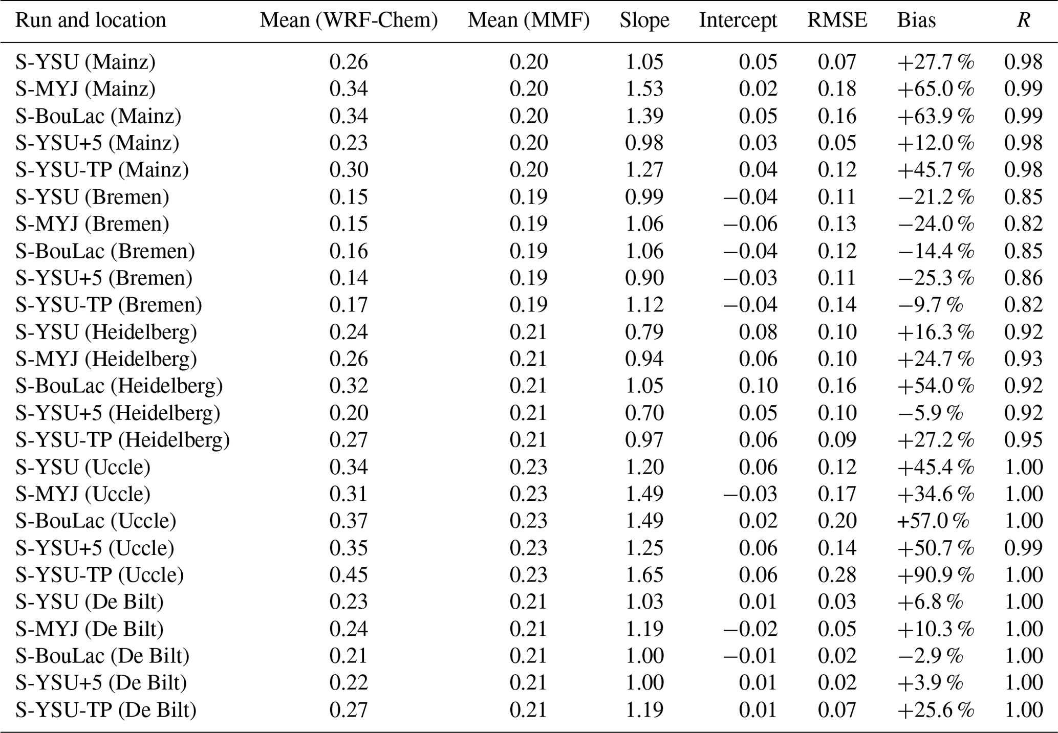
Mean, intercept, and RMSE are given in units of 10¹⁰ molec. cm⁻³.

4 Discussion and conclusion

We have presented new WRF-Chem simulation results with specific focus on NO₂. The simulations were run on a domain over central Europe with a spatial resolution of 3 km × 3 km for the month of May 2019. Over Germany, a new emission inventory from the German Environmental Agency with a resolution of 1 km × 1 km was used. Outside of Germany, the EDGARv5 emission inventory with a resolution of 11 km × 7 km was used. The obtained simulation results (surface concentrations, tropospheric columns, and concentration profiles) were compared to observational datasets. On the basis of this comparison, five different model setups were evaluated against each other. The five model runs differed by choice of the PBL scheme, an enhanced mixing approach according to Du et al. (2020), and tuning of the diurnal temporal emission profiles.

In Sect. 3.1 modelled NO₂ surface concentrations were compared to in situ measurements. The obtained results were qualitatively very similar to previously published literature (see Kuik et al., 2016; Poraicu et al., 2023), with a model bias of −15.7 % at noontime and +53.1 % at night. The noontime bias was minimized by correcting for the presumed NO_y cross sensitivities of the reference measurement using the correction term suggested by Lamsal et al. (2008) based on modelled volume mixing ratios of PAN and HNO₃, resulting in a noontime bias of +3.1 %. The night-time bias was found to be sensitive to the PBL scheme and was reduced to +23.8 % in a model run with the Bougeault–Lacarrere scheme. The best results were obtained by increasing the lower mixing threshold of the model, as described by Du et al. (2020). As expected from a vertically resolved examination of the model's mixing coefficients, the enhanced mixing approach mainly affected the surface layer of the model at night-time, where the model bias was reduced further to −3.1 %. An alternative approach to model bias reduction based on tuning the model's temporal emission profiles was introduced. By redistributing the model's NO_x emissions accordingly, a night-time bias of +27.7 % was obtained, while the noontime bias increased to +24.1 %. Optimizing the temporal profiles alone is therefore less promising than optimizing mixing because model-external validation of the chosen profiles cannot be provided at this point. Nonetheless, the study demonstrates how sensitive modelled surface NO₂ concentrations are to the temporal emission profiles. This is an important finding, seeing that significant corrections to the monthly or weekly temporal profiles were derived in model evaluation papers of the past (see, e.g. Poraicu et al., 2023; Kumar et al., 2021), implying that corresponding uncertainties should be assumed for the diurnal profiles (and in consequence, the model results) as well. The ${\mathrm{NO}}_{\mathrm{2}}/{\mathrm{NO}}_x$ ratios in the model could be improved by investigating other chemical mechanisms, photolysis schemes, and speciation profiles in sensitivity studies similar to those presented in our study.

In Sect. 3.2 modelled tropospheric NO₂ VCDs were compared to TROPOMI measurements. In order to make a representative comparison, the air mass factors of the TROPOMI retrieval were recomputed using the high-resolution NO₂ profiles from our simulation. The distribution of modelled and observed NO₂ VCDs was found to be similar and agrees with previously reported simulation results. It was shown that the model tends to overestimate the NO₂ VCDs and surface concentrations in similar geographic regions, e.g. in the strongly polluted regions of western Germany and the Netherlands. The five different model setups were shown to perform similarly well in the evaluation against satellite data, with biases between +3.0 % and +13.8 %, RMSE values of 0.80×10¹⁵ to 1.14×10¹⁵ molec cm⁻², and R values between 0.87 and 0.89. The model run with enhanced mixing showed reduced bias over the polluted regions of western Germany, whereas the model run with tuned temporal emission profiles showed stronger overestimations and performed worst overall. The results of Sect. 3.2 can be seen as a validation in favour of the model run with enhanced mixing. An important finding of the study is the overall weak sensitivity of the modelled NO₂ VCD to the choice of model parameters because it demonstrates that good general agreement with satellite data alone is not sufficient for the validation of a WRF-Chem simulation.

In Sect. 3.3 modelled noontime NO₂ concentration profiles were compared to profiles from MAX-DOAS measurements at five locations in central Europe from the FRM4DOAS network. The inversion algorithms MMF and MAPA were used. The level of agreement between simulations and observations varied from location to location. In most locations, the overall shape of the profile was reproduced well, but (mostly positive) biases occurred. The model run with enhanced mixing, which performed best in the remaining comparisons, showed biases of +12.0 % (Mainz), −25.3 % (Bremen), −5.9 % (Heidelberg), +50.7 % (Uccle), and +3.9 % (De Bilt). Two main qualitative differences between observed and simulated profiles were identified. First, the simulated profiles showed steep NO₂ gradients close to the surface and agreed well with the co-located surface concentration measurements. The observed profiles did not resolve the surface layer well, most likely due to the coarse retrieval grid with 200 m layer height. As a consequence, the observed profiles tended to underestimate the surface concentration measurements. Second, elevated NO₂ layers were found in some of the observed profiles but not in the corresponding simulated profiles. Here, the lack of vertical emission profiles, the overall spatial resolution of our WRF-Chem simulations, and the influence of horizontal concentration gradients on the MAX-DOAS inversion procedure were identified as possible explanations.

For future research, a definite statement on the issue of NO_y cross sensitivities of in situ measurements should be given by the UBA. The WRF-Chem modelling community should reconsider the current use of clipping thresholds for the mixing coefficients, seeing that their implementation is not transparent to the user and it is unclear how their original values were obtained. The parameterization should at least be made accessible through the namelist interface. In addition to the modification of the vertical mixing scheme, a combined optimization of mixing and temporal profiles also seems promising and should be tested in the future. Introduction of vertical emission profiles could potentially yield better agreement with MAX-DOAS measurements but likely requires re-adjustments of the lower mixing thresholds, which were deducted for simulations without vertically distributed emissions. Further model validations could be drawn from running the WRF-Chem simulation at the spatial resolution of the emission inventory. At least over Germany, where emission data with a resolution of 1 km × 1 km are available, the model resolution could in theory be increased by a factor of 9. It is possible that at such resolutions, the “traffic” measurement stations, which were dismissed in this study, can be used in a sensible way. However, this would realistically require us to shrink the geographical extent of the model domains. The feasibility of tuning the temporal emission profiles could be re-evaluated with the help of geostationary satellites, e.g. GEMS (Kim et al., 2020), Sentinel-4 (Stark et al., 2013), and TEMPO (Naeger et al., 2021). With an hourly measurement frequency, diurnal emission profiles could be derived with broad geospatial coverage and used for validation. Furthermore, the results of Sect. 3.2 would be much more informative if satellite observations were available for different hours of the day. The synergistic use of next-generation satellites and RCT models of much higher resolution has promising potential to expand the studies presented in this article.

Appendix A: Additional figures and tables

Table A1 Layer extent of the lowest 24 layers in our WRF-Chem simulation.

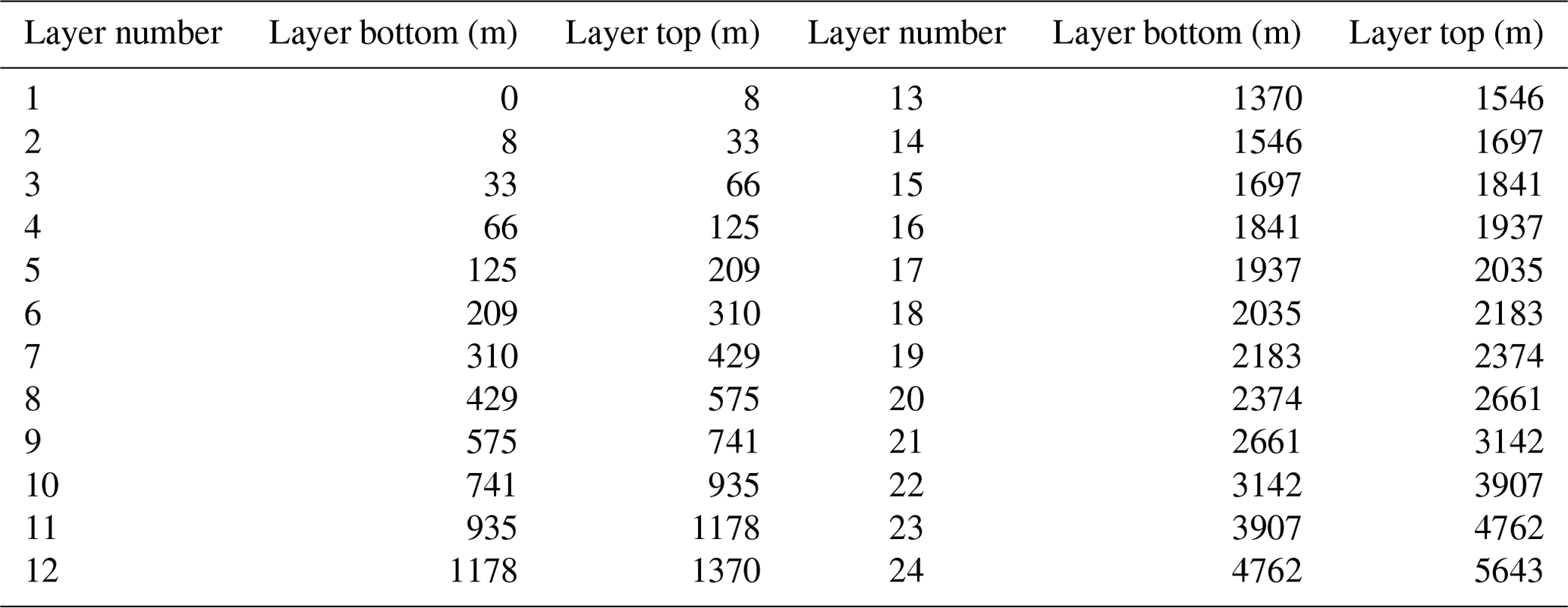
Exact layer bottoms and tops depend on location and time. The values given here are averages.

Figure A1 Like Fig. 3 but for traffic stations instead of background stations.

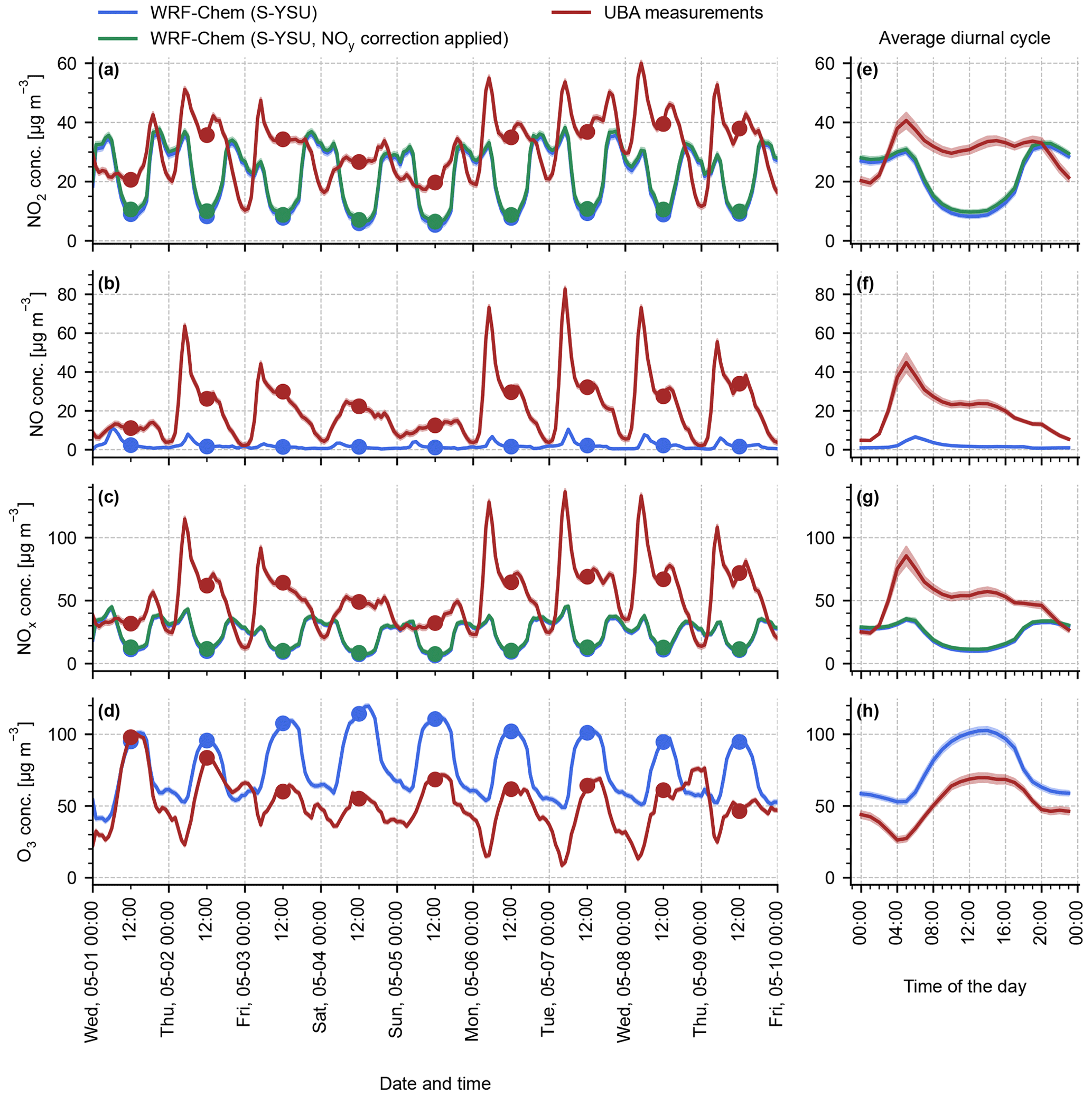
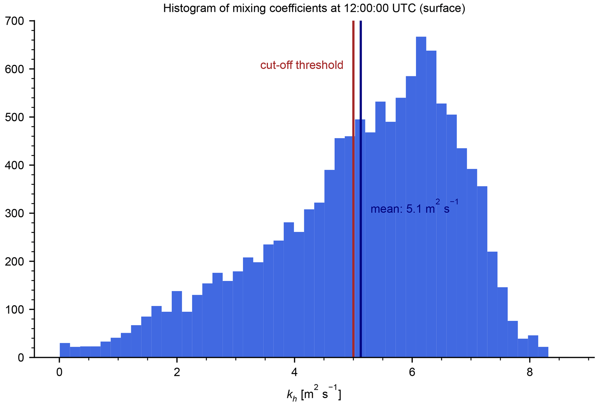
Figure A2 Histogram of the mixing coefficients used to produce the average values displayed in Fig. 6 for the simulation run S-YSU at noontime.

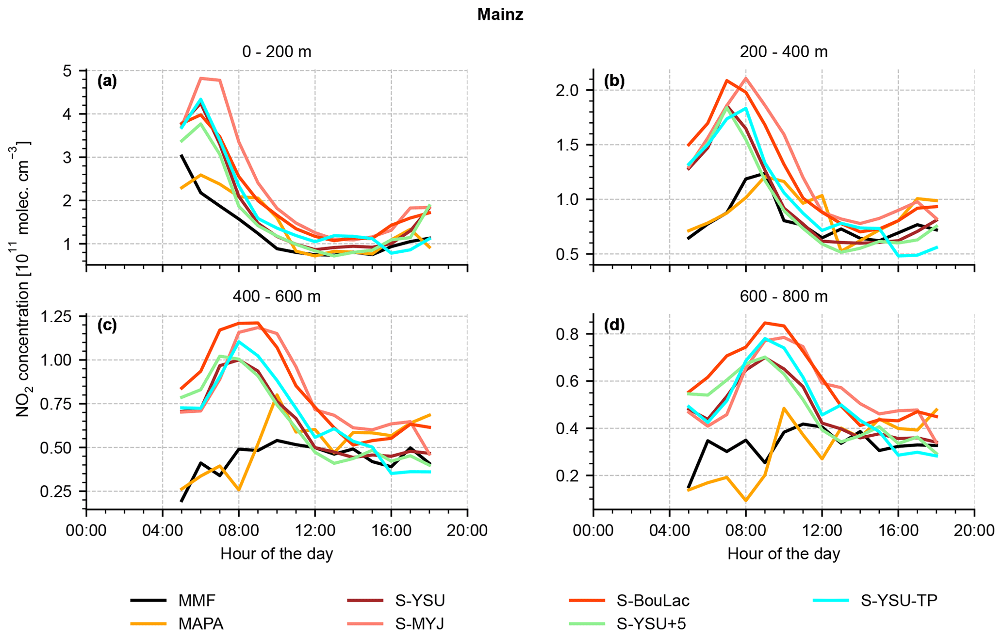
Figure A3 Temporally resolved comparison between NO₂ concentration profiles from MAX-DOAS measurements in Mainz, Germany, and simulated profiles from WRF-Chem. Here, only the first four layers of the MAX-DOAS retrieval are shown, with one layer per subplot.

Figure A4 Like Fig. A3 but for Bremen, Germany.

Figure A5 Like Fig. A3 but for Heidelberg, Germany.

Figure A6 Like Fig. A3 but for Uccle, Belgium.

Figure A7 Like Fig. A3 but for De Bilt, Netherlands.