Observationally constrained analysis of sulfur cycle in the marine atmosphere with NASA ATom measurements and AeroCom model simulations

The atmospheric sulfur cycle plays a key role in air quality, climate, and ecosystems, such as pollution, radiative forcing, new particle formation, and acid rain. In this study, we compare the spatially and temporally resolved measurements from the NASA Atmospheric Tomography (ATom) mission with simulations from five AeroCom III models for four sulfur species (dimethyl sulfide (DMS), sulfur dioxide (SO₂), particulate methanesulfonate (MSA), and particulate sulfate (SO₄)). We focus on remote regions over the Pacific, Atlantic, and Southern oceans from near the surface to ∼ 12 km altitude range covering all four seasons. In general, the differences among model results can be greater than 1 order of magnitude. Comparing with observations, model-simulated SO₂ is generally low, whereas SO₄ is generally high. Simulated DMS concentrations near the sea surface exceed observed levels by a factor of 5 in most cases, suggesting potential overestimation of DMS emissions in all models. With GEOS model simulations of tagging emission from anthropogenic, biomass burning, volcanic, and oceanic sources, we find that anthropogenic emissions are the dominant source of sulfate aerosol (40 %–60 % of the total amount) in the ATom measurements at almost all altitudes, followed by volcanic emissions (18 %–32 %) and oceanic sources (16 %–32 %). Similar source contributions can also be derived at broad ocean basins and on monthly scales, indicating the representativeness of ATom measurements for global ocean. Our work presents the first assessment of AeroCom sulfur study using ATom measurements, providing directions for improving sulfate simulations, which remain the largest uncertainty in radiative forcing estimates in aerosol climate models.

1 Introduction

Atmospheric sulfur species have wide-ranging environmental and health impacts. About two-third of sulfur emissions come from anthropogenic activities (Chin et al., 2000); therefore, considerable efforts have been made to reduce these sulfur emissions. For example, acid rain occurs when sulfur dioxide (SO₂) is oxidized to form sulfuric acid and particulate sulfate (SO₄), which fall to the ground with the rain (Bian et al., 1993; Grennfelt et al., 2020) and can devastate aquatic ecosystems (Josephson et al., 2014; McDonnell et al., 2021). Through the competing neutralization reaction of SO₄ and nitrate with NH₃ and other alkaline species, SO₄ affects strongly both particulate nitrate formation (Bian et al., 2017) and aerosol pH (Huang et al., 2020; Nault et al., 2021). Sulfate is a key component of particulate matter (PM), which degrades air quality (Dong et al., 2018; Tan et al., 2018) and directly reflects the solar radiation (Moch et al., 2022; Myhre et al., 2013). Due to its highly hygroscopic nature, sulfate aerosols act as efficient cloud condensation nuclei (Boucher et al., 2013; Breen et al., 2021; Seinfeld et al., 2016) and thus indirectly radiative forcing (Penner et al., 2016; Wang et al., 2021) through aerosol–cloud interactions. The contribution of aerosols to atmospheric clouds and the energy budget remains the largest uncertainty in climate models (Gryspeerdt et al., 2023; Jia et al., 2021, 2022; Klein et al., 2013; Malavelle et al., 2017). Sulfate is important primarily because the atmospheric sulfate component itself contributes to radiative forcing (RF) almost as much as all other major non-natural aerosol components, as concluded from 16 AeroCom model studies (Myhre et al., 2013). More importantly, uncertainty in sulfate simulations in current climate models is a major contributor to biases in aerosol optical depth (AOD; Fig. 3 in Gliß et al., 2021) and RF (Fig. 7 in Myhre et al., 2013).

Unlike other major atmospheric aerosols, a significant fraction (i.e., roughly a quarter) of sulfate in the atmosphere comes from marine biological emissions (Chin et al., 1996). The impact of oceanic sulfate is particularly pronounced on marine shallow clouds, which are characterized by low droplet number concentrations and weak updraft velocities (Rissman et al., 2004). Sulfur research has also focused on the tropical upper troposphere (TUT), where the growth of new aerosol particles and homogeneous nucleation involving sulfuric acid is at a maximum (Williamson et al., 2019) and where deep convective transport allows a small portion of the sources to reach the lower stratosphere. The resulting sulfate aerosols in the stratosphere can persist for years (Holton et al., 1995). Unfortunately, the observations in the TUT region and above are sparse. Acquiring atmospheric composition and its chemical and physical properties over remote oceans is challenging, although satellites can often provide total column constraints of aerosol optical depth.

The NASA Earth Venture Suborbital (EVS-2) Atmospheric Tomography (ATom) airborne mission provided abundant measurements of gases and aerosols over the world's oceans (Hodzic et al., 2020; Thompson et al., 2022). In particular, a suite of instruments integrated on the NASA Douglas DC-8 jetliner (hereafter DC-8) made measurements of many important sulfur species including dimethyl sulfide (DMS), SO₂, particulate methanesulfonate (MSA), and SO₄ over the Pacific and Atlantic oceans in both hemispheres and the Southern Ocean in all four seasons. These regions provide us with highly heterogeneous natural and anthropogenic source environments, which is not usually the case for traditional continental studies. The comprehensive ATom sulfur dataset provides us with unprecedented opportunities to assess sulfur source, transport, chemistry, deposition, and particle activation and growth represented in the global aerosol models, as well as to estimate the extent of the anthropogenic influence on remote oceanic atmospheric composition and cloud properties.

This study has two specific scientific goals. First, we explore the vertical and seasonal variation in sulfur species (i.e., DMS, SO₂, MSA, and SO₄) using ATom measurements and simulations from five global models that participated in the AeroCom–ATom model experiments. AeroCom is an international initiative of scientists aiming at the advancement of the understanding of global aerosol and its impact on climate (https://aerocom.met.no/, last access: 1 February 2024). Here we focus on remote regions over the Pacific, Atlantic, and Southern oceans, from near the surface to an altitude of about 12 km, covering all four seasons. Second, we determine whether the produced SO₄ originated from anthropogenic or natural sources by using tagged tracers associated with emission types.

Our work is the first study to use ATom measurements for comparison with the AeroCom models, focusing on all sulfur species simulated in current aerosol climate models. This work extends previous efforts using ATom measurements to evaluate the organic carbon (Hodzic et al., 2020) and black carbon (Katich et al., 2018) of AeroCom models, as well as individual models focusing on new particle formation in the tropics (Williamson et al., 2019), fine aerosol lifetime (Gao al. al., 2022), aerosol vertical transport (Yu et al., 2019), sea salt (Bian et al., 2019), smoke (Schill et al., 2020), mineral dust (Froyd et al., 2022), and DMS chemistry (Fung et al., 2022). Furthermore, to our knowledge, there are no studies that systematically investigate the changes and sources of all major sulfur species over the remote ocean. Our study aims not only to reveal sulfur variability based on multiple measurements and model simulations, but also to tease out the underlying processes behind the variability through a comprehensive analysis of simulated sulfur species in aerosol climate models.

The structure of this paper is as follows. Section 2 describes the ATom measurements and the AeroCom models used in this study. Section 3 presents the ATom–AeroCom sulfur comparison from different perspectives, namely the overall comparison in Sect. 3.1, the vertical profiles in Sect. 3.2, and the regional and seasonal analysis in Sect. 3.3. The sulfur budget analysis is given in Sect. 4. We further present investigations of source origins for aerosol SO₄ along flight tracks and over oceans in Sect. 5. Finally, we summarize our findings in Sect. 6.

2 Data

2.1 ATom measurements

ATom was a NASA-funded Earth Venture Suborbital project designed to study the effects of air pollution on chemically reactive gases, aerosols, and greenhouse gases in the remote atmosphere. ATom deployed a large suite of gas and aerosol measurement instruments on the NASA DC-8 aircraft for systematic sampling, covering an extended region of the globe from 85^∘ N to 85^∘ S over the Pacific and Atlantic oceans, with vertical profiles from near the surface to the near tropopause (i.e., 0.2–12 km; Thompson et al., 2022). Four ATom deployments (ATom-1 to ATom-4) were executed over each of the four seasons from 2016 to 2018, and their flight paths are shown in Fig. 1. The extensive aerosol and gas measurements made during ATom include inorganic and organic aerosols, precursor gases, particle size distributions, and particle composition. Table 1 lists the instruments for ATom sulfur species observations used in this study including the relevant sampling details needed for the model comparison.

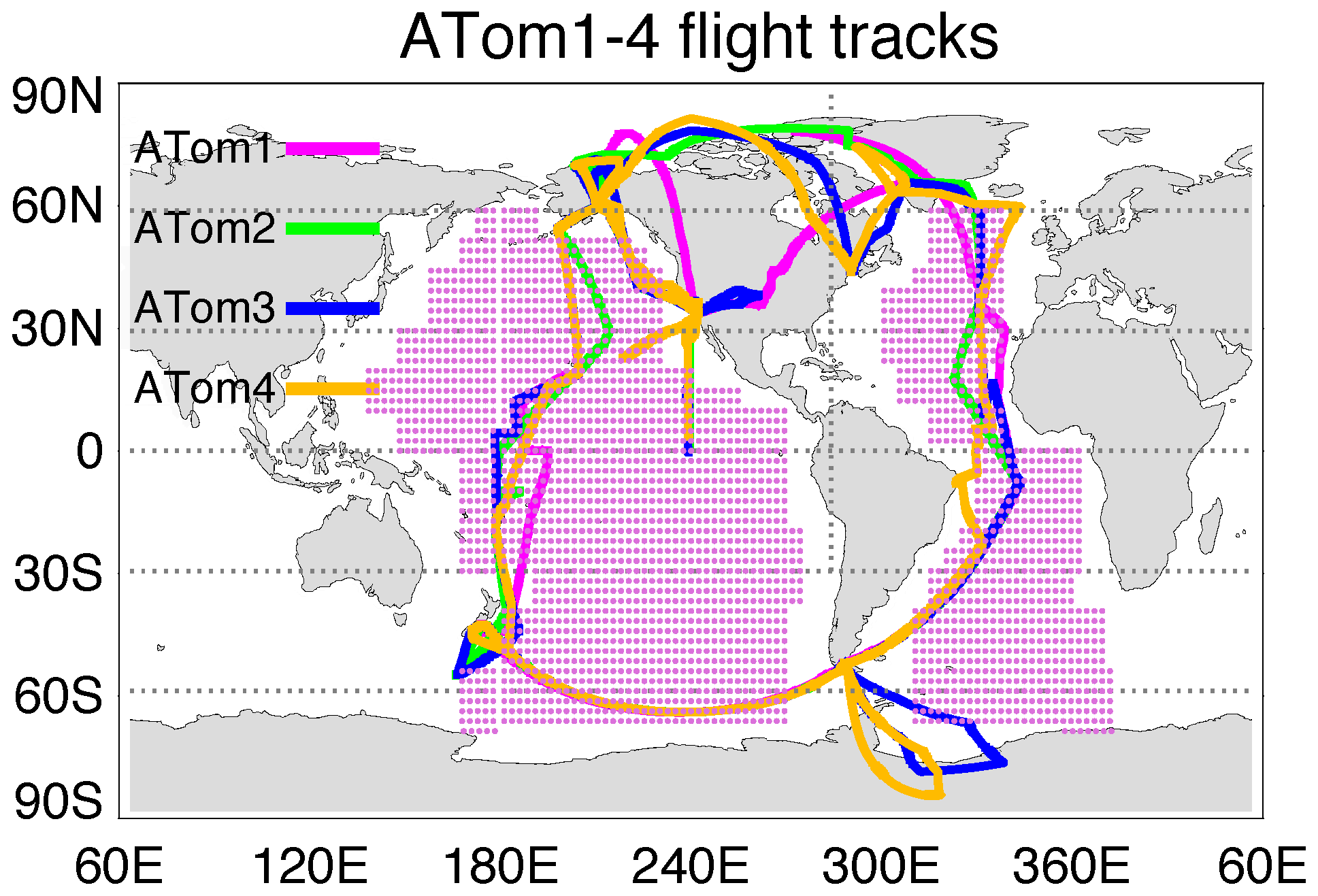
Figure 1 Flight tracks of ATom-1 to ATom-4 and regions for the analysis of SO₄ source origins (shaded area). Periods of the four ATom deployments are ATom-1 (July–August 2016), ATom-2 (January–February 2017), ATom-3 (September–October 2017), and ATom-4 (April–May 2018).

Table 1 ATom sulfur measurements used in the study.

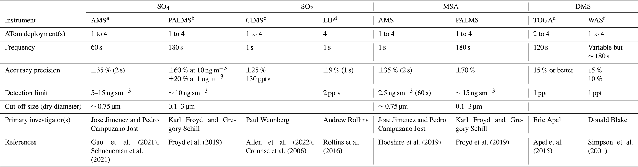
^a AMS: aerosol mass spectrometer. ^b PALMS: particle analysis by laser mass spectrometer. ^c CIMS: chemical ionization mass spectrometer. ^d LIF: laser-induced fluorescence. ^e TOGA: NCAR trace organic gas analyzer. ^f WAS: whole air sampler.

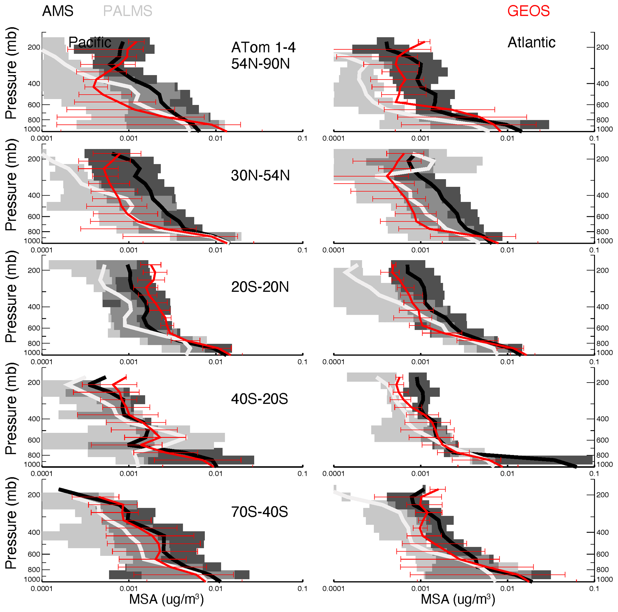
We use SO₄ and MSA that had been measured by two instruments, the University of Colorado Aerodyne high-resolution time-of-flight aerosol mass spectrometer (AMS; Canagaratna et al., 2007; Guo et al., 2021) and the NOAA particle analysis by laser mass spectrometer (PALMS; Froyd et al., 2019). The latter makes in situ measurements of the chemical composition of individual aerosol particles. Furthermore, AMS measured submicron aerosols, while PALMS provided mass mixing ratios and size distributions up to 3 µm in dry diameter (Brock et al., 2019). It is worth noting that AMS data were independently processed and reported at both 1 and 60 s time resolutions by the instrument PI (Jimenez et al., 2019). The detection limit varied with different averaging time resolutions, and they were provided directly for each sampling point in AMS datasets. Some negative measurements were also presented in AMS datasets, and this is normal for measurements of very low concentrations in the presence of instrumental noise. The AMS data at 60 s resolution are recommended owing to more robust peak fitting at low concentrations (Hodzic et al., 2020). Given the complex data overlays (i.e., starting, ending, and frequency) reported from multiple instruments, the ATom team also provide a 10 s merged dataset to facilitate users' applications. In this study, we evaluate data reported in different time resolutions, using AMS as an example, to ensure the quality of merged data that are exclusively used as the primary dataset in this work.

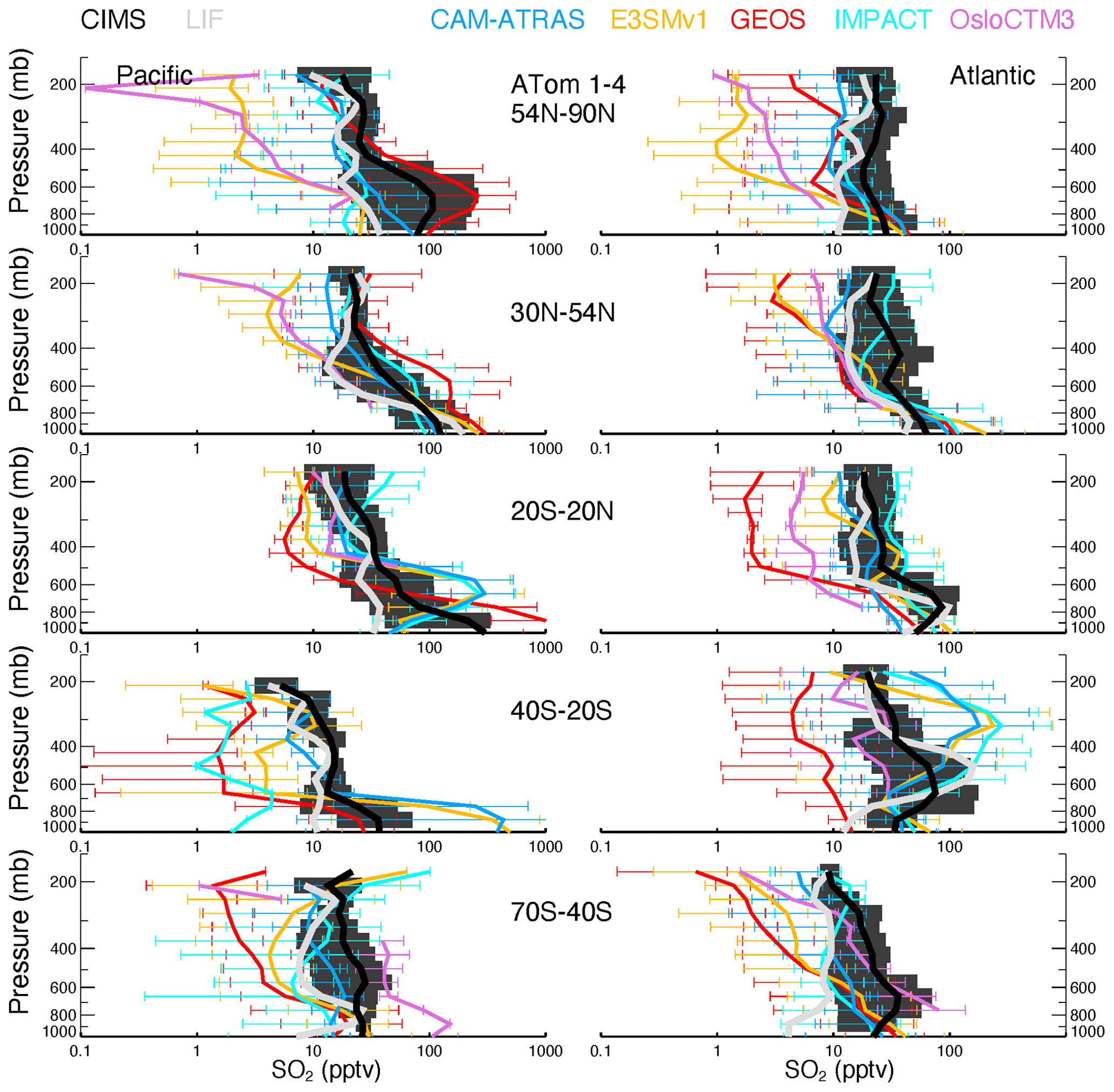
Two instruments were used for SO₂ measurements: the California Institute of Technology chemical ionization mass spectrometer (CIMS) and the NOAA laser-induced fluorescence (LIF) instrument (Table 1). The CIMS uses CF₃O⁻ as a reagent ion which reacts with SO₂ via fluoride ion transfer chemistry. The product ion is detected by a compact time-of-flight mass spectrometer (CToF). The precision of the CIMS SO₂ measurement decreases with increasing water vapor concentration (Eger et al., 2019; Huey et al., 2004; Jurkat et al., 2016; Rickly et al., 2021), making it challenging to measure SO₂ in remote ocean regions. In these regions, the ambient water vapor may be sufficiently high that the CIMS SO₂ precision at 1 s resolution (∼ 130 parts per trillion by volume, pptv) is insufficient for measuring ambient SO₂ values there (< 100 pptv). To address this shortcoming, the ATom science team added a new instrument, the NOAA LIF instrument, to the ATom-4 payload. The NOAA LIF instrument uses red-shifted laser-induced fluorescence to detect SO₂ at very low parts per trillion levels (Rickly et al., 2021; Rollins et al., 2016). Both instruments report negative values, and the detection limit of the LIF instrument is about 2 pptv.

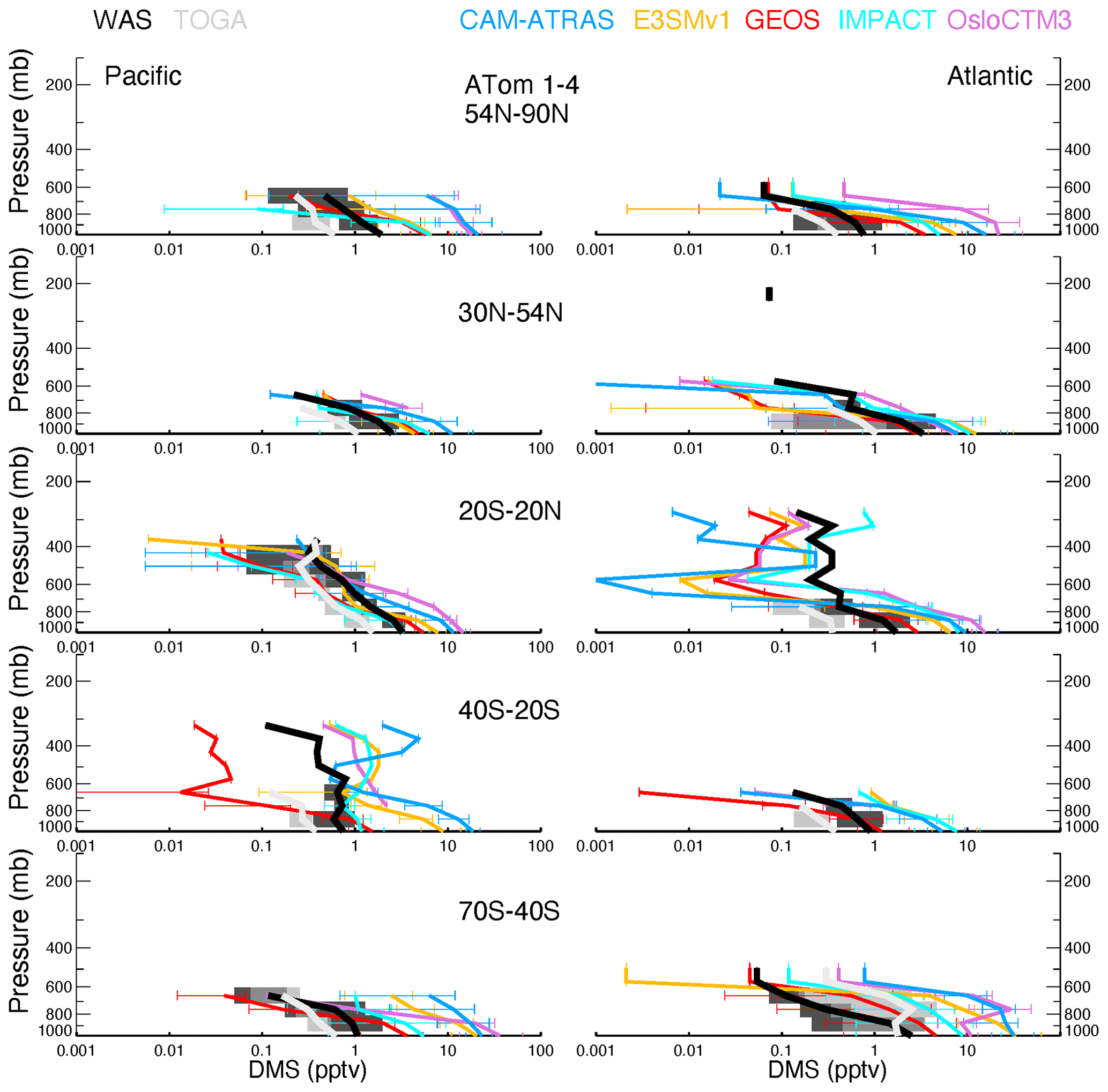
DMS was measured during ATom by two instruments: the University of California, Irvine, whole air sampler (WAS) and the NCAR trace organic gas analyzer (TOGA). The WAS reported DMS for all four ATom deployments, while the TOGA reported data for ATom-2 to ATom-4 and not for ATom-1 due to possible issues associated with the TOGA inlet (the inlet was changed for ATom-2 to ATom-4). Both instruments have a comparable detection limit (1 pptv) and accuracy (∼ 15 %). However, the sampling time interval of the WAS (variable but ∼ 180s) was longer than the TOGA (∼ 120 s).

2.2 AeroCom models

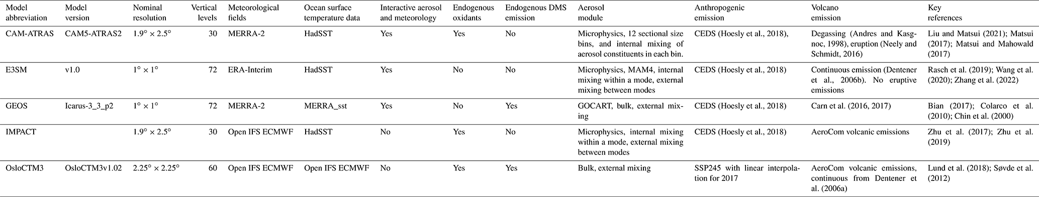
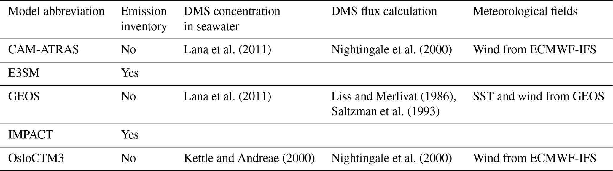
Five global aerosol models participated in an AeroCom–ATom model experiment (https://wiki.met.no/aerocom/phase3-experiments, last access: 1 February 2024): CAM-ATRAS, E3SM, GEOS, IMPACT, and OsloCTM3. The experiment required all participating models to (1) conduct 3-year simulations of 2016–2018 (i.e., covering the whole ATom observation period), (2) use or nudge meteorological data for the simulation period, and (3) use the same pre-defined emission fields for precursor gases and aerosol tracers. The suggested emissions are the Coupled Model Intercomparison Project Phase 6 Community Emissions Data System (CEDS; Hoesly et al., 2018) for anthropogenic sources, daily biomass burning emission (such as the Global Fire Assimilation System, GFAS), a dataset based on satellite volcanic SO₂ observations from the OMI instrument on the Aura satellite (Carn et al., 2016, 2017) for outgassing and eruptive volcanic emission, and DMS concentration in sea surface from Lana et al. (2011). Wind-driven emissions, such as dust and sea salt, are calculated online by each model. Table 2 summarizes the detailed model characteristics and input datasets relevant to this study. It is worth noting that CEDS specifies anthropogenic emissions from various sectors, including emissions from shipping. The version of CEDS used in this work has emissions up to 2014, and all models use the 2014 emissions for ATom periods. Furthermore, unlike other models that use CEDS emissions, the anthropogenic emissions of OsloCTM3 are obtained following Shared Socioeconomic Pathways (SSP) under the Representative Concentration Pathway (RCP) scenario with medium radiative forcing by the end of the century (SSP245; Fricko et al., 2017), and the emissions are interpolated to 2016 and 2017. Following the experimental protocol, all models provided results for all ATom periods except for OsloCTM3 that omitted data in ATom-4. Unlike traditional AeroCom experiments that used gridded daily/monthly averaged data, modelers are required to interpolate model results along the flight track every 10 s (see more discussion in Sect. 3.1) using three-dimensional high-frequency (e.g., hourly or even less depending on the models' time step) data to facilitate the comparison. It is worth noting that the models do not have any actual information at 10 s time resolution, given their time steps are at least 10× greater and their spatial resolutions are coarse. However, the interpolation methodology suggested here provides the best model information at their current configuration to compare with aircraft measurements.

Table 2 AeroCom models used in this study.

The AeroCom–ATom experiment also designed three sensitivity simulations by tracking gas and aerosol emissions to anthropogenic, biomass burning, and volcanic sources to attribute the origin of sulfur sources in sulfur simulations over remote oceans. These experiments were conducted with the Goddard Earth Observing System (GEOS) model. The setup of the GEOS model followed the experiment protocol generally, but GEOS used its own daily biomass burning emissions that were derived from the Quick Fire Emissions Dataset (QFED) developed based on MODIS fire radiative power and calculated in near real-time at 0.1^∘ resolution (Darmenov and da Silva, 2015; Pan et al., 2020). Emissions from biogenic sources were calculated using the Model for Emissions of Gases and Aerosols from Nature (MEGAN) embedded in the GEOS model.

2.3 Tagged-tracer study in GEOS

Tagged-tracers or tags are tied to sources of selected emission types and/or emission locations. Such a tag isolates plumes from certain activities and is a powerful tool to help understand source attribution or diagnose model performance at the process level. The mechanism behind this technique is that each specific aerosol component in GEOS GOCART is modeled independently of the other components, and the contribution of each emission type to the total aerosol mass is not disturbed by the other emission types. Therefore, additional aerosol tracers can be easily “tagged” to capture emission type (e.g., anthropogenic, biomass burning) and location (local, regional, or global scale). Tags can be multi-instantiated and computed simultaneously with their baseline counterparts, thereby increasing the computational efficiency of the aerosol models.

The tagged-tracer technique in GEOS has been widely used in aerosol and gas studies (Bian et al., 2021; Nielsen et al., 2017; Strode et al., 2018) and in supporting various aircraft field campaigns such as Arctic Research of the Composition of the Troposphere from Aircraft and Satellites (ARCTAS) and ATom. Such techniques are also adopted in other models such as the GEOS-Chem model (Fisher et al., 2017; Ikeda et al., 2017; Lin et al., 2020) and Community Earth System Model (CESM; Butler et al., 2018).

Four tags linked to emission types of anthropogenic, biomass burning, volcanic, and marine emissions were used in the GEOS model to identify anthropogenic vs. natural sources of sulfate, and the results are discussed in Sect. 5.

3 ATom–AeroCom comparisons of sulfur species

This section presents a comparison of sulfur species between ATom measurements and AeroCom model simulations. The consistency and diversity of data across remote regimes, both horizontally and vertically, help us understand the effects of emissions, transport, and chemical transformations, as well as shed light on improving the processes in models to best represent the ATom observations.

3.1 Overall comparison

The overall performance of SO₄ probability density function (PDF) distribution observed from the AMS and PALMS instruments and simulated by five AeroCom models for four ATom deployments is presented in Fig. 2. Also shown in Fig. 2 are the various corresponding percentiles, namely, 0th (minimum), 25th, 50th (median), 75th, and 100th (maximum), and the mean for statistical analyses. The median and mean values are further given in Table S1. The ATom team provided a 10 s merged dataset deliberately by integrating data from various instruments to a unified temporal resolution. We use this 10 s merged dataset where observations are above the detection limit (DL) throughout the main text unless otherwise stated. When multiple instruments measured the target field, only points where all instruments measured above DL values were included in analysis, e.g., AMS 10 s in red and PALMS 10 s in gray in Fig. 2. All model results were sampled mimicking flight observations (see Sect. 2.2), and only data with measurements available were used in comparison. This approach ensures that model evaluation is based on high-quality measurements. It is worth noting that the given statistical values in this method represent more regions having high tracer concentration or mixing ratio. In the Supplement, we further give a model–observation comparison for all available measurement data including negatives.

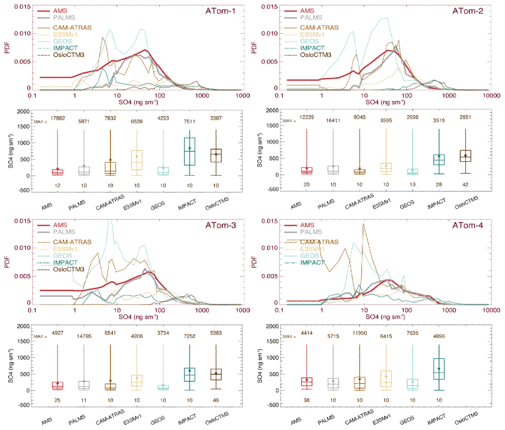
Figure 2 SO₄ probability density functions (PDFs) and its statistical values shown by box-and-whisker plots for the four ATom deployments. All data (AMS in red, PALMS in gray, and five model simulations in other colors) are sampled at 10 s points. Statistical values include the range of the data from minimum to maximum; the three levels of the 25th, 50th (median), and 75th percentiles in the box; and the filled circle for the mean. Statistical values are calculated when measured values are above the detection limit (DL).

The mean of PALMS SO₄ is generally about 10 %–50 % higher than AMS SO₄ across four ATom deployments. This performance may be attributed, at least in part, to the fact that the sample size range of PALMS (∼ 3 µm) is larger than that of AMS (∼ 0.75 µm), as mentioned in Sect. 2.1. However, the difference between the two observations is much smaller than the difference between observations and model. Clearly, the differences in simulated SO₄ among models are high and can easily exceed several orders of magnitude. Most observed and simulated SO₄ exhibits the highest probability density around SO₄ values of 10–100 ng sm⁻³. With the exception of GEOS and CAM-ATRAS, the model SO₄ PDFs show higher tails beyond 100 ng sm⁻³, which explains the higher median and mean SO₄ simulated by the models. Statistical analysis performed on selected percentiles (box-and-whisker plots in Fig. 2) indicates that multi-model SO₄ medians are about 3.7 (ATom-1), 2.2 (ATom-2), 1.9 (ATom-3), and 1.2 (ATom-4) times higher than those observed. In general, nearly all measurements and models indicate that SO₄ concentrations on a global ocean basis are highest during the Northern Hemisphere (NH) spring season (ATom-4). Similar analysis was also performed on all (e.g., both positive and negative) measurement data (Fig. S2), and the median and mean values of observations are naturally smaller than those in Fig. 2 by 8 %–20 %, but the PDF distributions are almost identical between the two treatments.

Figure 3 shows the PDF distribution and statistics for SO₂. All observed and simulated data were reprocessed by including points above the detection limit (2 pptv) only. Both instruments (CIMS and LIF) were deployed during ATom-4. Despite the CIMS being less precise than LIF (Rollins et al., 2016), both instruments agreed within 95 %, and CIMS-measured SO₂ concentrations were consistently 3 %–7 % lower than LIF measurements. This difference is within the combined uncertainties of the two measurements, but it suggests a systematic calibration difference that is currently unresolved (Rickly et al., 2021). Meanwhile, the width of the CIMS SO₂ PDF (measured at half-height) is narrower in ATom-4 than ATom-3 because of improved measurement precision in ATom-4. The CIMS resolution was improved in ATom-4, which enables a better separation of SO₂ and formate H₂O. The CIMS SO₂ PDF in ATom-4 is around 10 pptv and is more consistent with LIF measurements and model simulations. In contrast, the distribution of SO₂ measured by the CIMS during ATom-1 to ATom-3 is spread much wider than the models. Throughout ATom periods, models, especially E3SM, GEOS, and OsloCTM3, show higher peak heights and narrower peak widths. Statistics indicate lower model SO₂ medians than those observed (box-and-whisker plots in Fig. 3), especially during ATom-1. However, the model means are comparable to or even higher than those observed, indicating that the models simulate episode events that were not reported in measurements. Consequently, the simulated mean/median ratio is higher than the observed value. Among the four ATom deployments, ATom-4 has much better model observation consistency. Figure S3 presents the corresponding analysis, including the measured negative values. Compared to Fig. 3, the observed median and mean values drop substantially (up to 50 %).

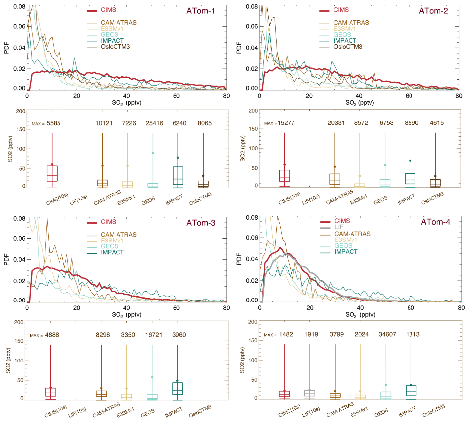
Figure 3 Similar to Fig. 2 but for SO₂. Observational data are CIMS (red) for ATom-1 to ATom-4 and LIF (gray) for ATom-4 from ATom 10 s merged data. PDFs and statistical values are calculated at points where CIMS-measured (and LIF-measured in ATom-4) SO₂ is above the DL (e.g., 2 pptv).

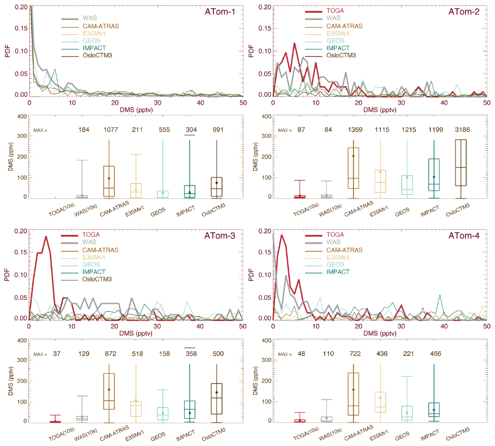
Figure 4 Similar to Fig. 2 but for DMS for ATom-1 to ATom-4. The original data reported by the TOGA (e.g., 35 s) and by the WAS (e.g., ∼ 60 s) have also been converted to 10 s frequency. Data included in PDFs and statistical analyses are on 10 s points where DMS values measured by both the TOGA and WAS are above the DL (i.e., 1 pptv).

Atmospheric DMS observations are scarce, especially on a global scale. Thus, DMS measurements by the two instruments (WAS and TOGA) during the four ATom deployments provide an unprecedented opportunity to investigate biological DMS over global remote oceans and evaluate model DMS simulations on spatial and temporal distributions. By excluding points with measured values below the detection limit (i.e., 1 pptv), the overall DMS comparison in Fig. 4 indicates the TOGA has higher data peaks and probability densities when DMS ranges from 3–10 pptv. However, this does not appear to be consistent with the lower median and mean values of the TOGA, indicating a higher tail in the WAS DMS PDF. Likewise, although the peak of the WAS DMS PDF is significantly higher than all models from 3–10 pptv (∼ 5–20 pptv for ATom-3), the median and mean of the WAS DMS are lower, suggesting an even higher tail in the model DMS PDF. Overall, there is a big gap between the WAS and TOGA DMS measurements, and both are surprisingly low compared to the models. Statistical analysis performed on selected percentiles (the box-and-whisker plots) indicates that multi-model DMS medians are about 4.9 (ATom-1), 8.6 (ATom-2), 6.6 (ATom-3), and 7.7 (ATom-4) times higher than those observed, while model GEOS has a better performance (i.e., 1.2, 2.7, 2.3, and 2.8 correspondingly). The model DMS median values are mostly higher than the observed values. The model DMS mean values are even higher than the observed means (sometimes by more than a factor of 10). This reflects a few very high predicted DMS values. Based on what we know about DMS sources and sinks, these very large simulated DMS values appear most commonly in the boundary layer (BL). Indeed it is confirmed in Fig. 5 by looking at the ratios of DMS median values between model simulations and observations. The analyses are performed on four vertical ranges (e.g., the entire vertical column, the BL 0–1.5 km, the low–middle free troposphere 1.5–6 km, and the upper troposphere 6–12 km). The last column “MMM/MOM” refers to multi-model median to multi-observation median. The high ratio stems mostly from the BL, above which the consistency is much better. Meanwhile, the PDF distribution and statistics of the models agree better with the WAS measurement than with the TOGA measurement. We should also acknowledge that this is a very limited set of observations we used here and that there are some longer-term DMS observations near the surface that were used as input for the parameterization of DMS emissions. More DMS observations near the ocean surface are needed to make a confident comparison.

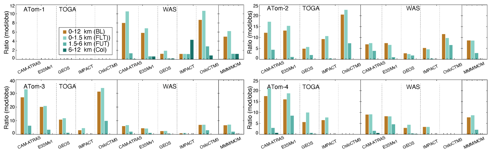
Figure 5 Ratio of DMS median values between model simulations and observations for four ATom deployments. Ratio analyses are performed on four vertical ranges as shown in four colors (see legend in ATom-1). The last column “MMM/MOM” refers to multi-model median to multi-observation median.

3.2 Vertical profiles

Vertical profiles of ATom-1 to ATom-4 for observed and modeled SO₄, SO₂, DMS, and MSA are shown in Figs. 6–9, respectively, for five latitude bands (from the north to the south) and for both the Pacific Ocean and Atlantic Ocean basins. Again, the profiles include equal amounts of data for each measurement and model result. In other words, all comparisons show only available points where the two observed values (i.e., AMS vs. PALMS for SO₄ and MSA, CIMS vs. LIF for SO₂, and TOGA vs. WAS for DMS) are greater than their detection limits and where the model values are extracted.

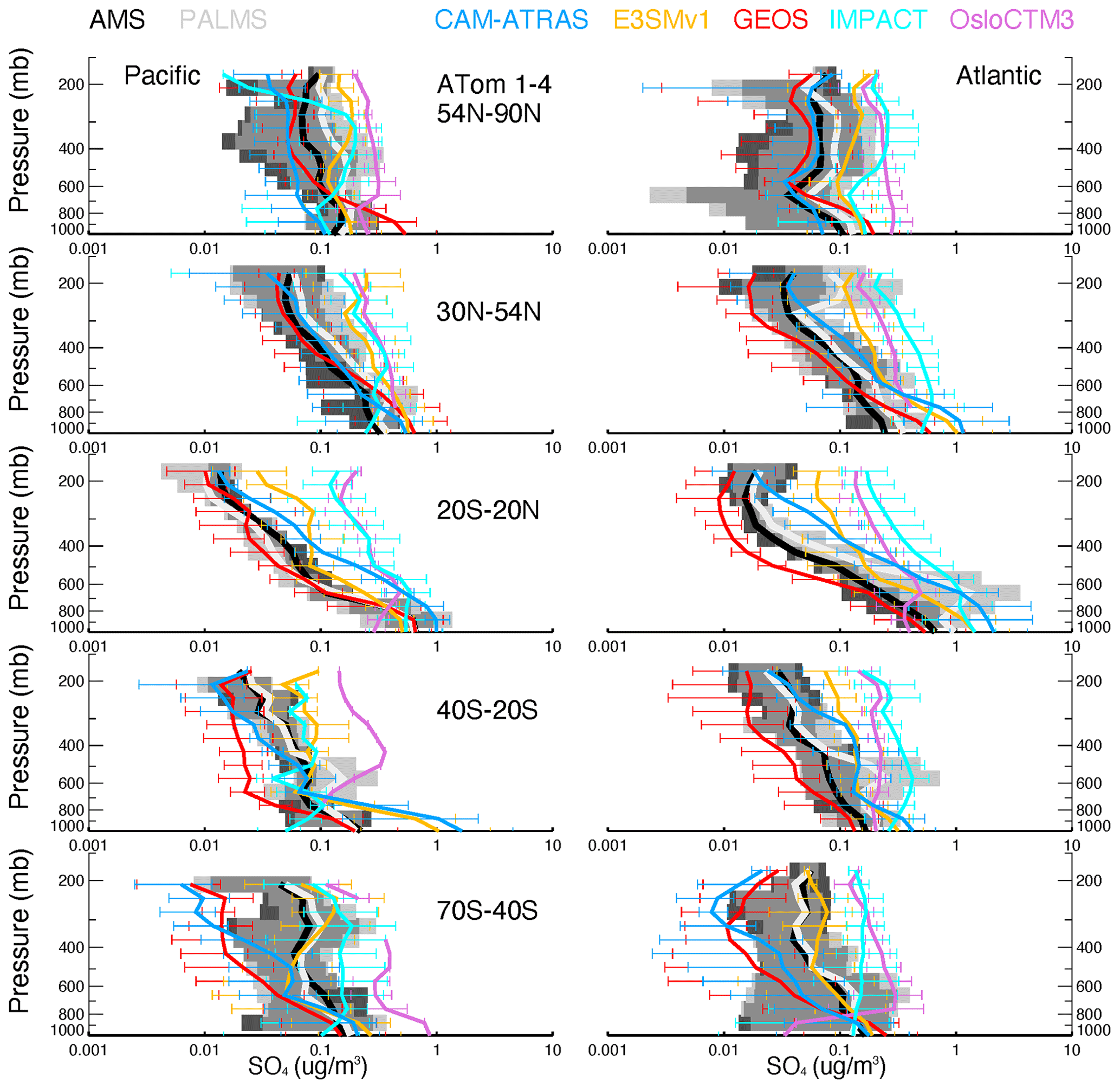
Figure 6 Observed and modeled vertical profiles of SO₄ in 1 km vertical bins averaged for four ATom deployments (lines) and variation across the four deployments (shaded area for measurements and horizontal bars for simulations). ATom measurements are shown in black (AMS) and light gray (PALMS), while model results are shown in other colors. Comparisons are conducted only when both observational measurements above the detection limit are available. Comparisons are separated into five latitude bands from the Northern Hemisphere to the Southern Hemisphere and into Pacific and Atlantic basins.

The average and range of sulfur tracers for ATom-1 to ATom-4 are shown in Figs. 6–9, and their corresponding details in each ATom period are further given in Figs. S5–S8. As shown in Fig. 6, the SO₄ values measured by the two instruments are close to each other and lie generally within the range of modeled SO₄ throughout the ATom periods. The spread of modeled SO₄ concentrations is large, exceeding an order of magnitude, especially in the upper troposphere. Despite the need for improvements, the models are generally able to capture the shape of the SO₄ profile. Specifically, CAM-ATRAS and GEOS have good SO₄ vertical gradients over the tropical and NH oceans, but their SO₄ values are too low compared to measurements over the Southern Hemisphere (SH) free troposphere. The SO₄ of IMPACT and OsloCTM3 decreases too slowly with altitude, as shown by their overestimated SO₄ values at high altitudes globally. The results of E3SM are generally within the ranges predicted by the other models. However, the performance of these models' SO₄ vertical profiles cannot simply be explained by the way the oxidant is applied because among the five models, CAM-ATRAS, IMPACT, and OsloCTM3 used interactive oxidant calculations, while E3SM and GEOS used archived oxidant data (Table 2). Of the five models, OsloCTM3 and GEOS participated in the multi-model OH assessment (Nicely et al., 2020) and OsloCTM3 had a shorter methane lifetime (relative to OH) than GEOS.

Figure 7 shows generally lower modeled SO₂ volume mixing ratios compared to the CIMS observations for most altitudes and latitude bins. The spread among modeled SO₂ values exceeds an order of magnitude around the measured SO₂. SO₂ is better simulated by the IMPACT model in the NH than the other four AeroCom models and by the CAM-ATRAS and OsloCTM3 models in the SH than the other three AeroCom models. The tropical Pacific appears to be an interesting region, with all models except GEOS failing to capture observed local SO₂ sources. Basically, the observed SO₂ is high at the surface, falls rapidly in the BL, and then gradually decreases above the BL, except for ATom-1, during which a second peak appears just above the BL (see Fig. S6 for the details of ATom-1 to ATom-4 separately). These observations indicate a strong local source for SO₂ in all seasons and a transport source in the NH summer in the lower free troposphere (ATom-1). Like observations, the model GEOS predicts a local source for SO₂ at the surface, but it misses the plume above the BL in ATom-1, and its vertical SO₂ convection is consistently too weak. Since only one flight was in ATom-1, more observations are needed to confirm whether GEOS has been failing to catch the plume there during the NH summer. All other models show lower SO₂ at the surface than in the lower free troposphere, which is inconsistent with the observed profiles. Figure S6 also shows an excellent agreement of SO₂ profiles measured by the CIMS and LIF during ATom-4, and models agree with measurements better in ATom-4 as well.

Figure 7 Similar to Fig. 6, but for SO₂. Note LIF (light gray) was deployed only in ATom-4.

DMS measurements fill in another piece of the puzzle for the atmospheric sulfur budget. As shown in Fig. 8, all five AeroCom models generally overestimate DMS in the BL, particularly for models CAM-ATRAS and OsloCTM3. This large bias close to the surface requires us to revisit the DMS emissions employed in our models. Of the five models, DMS emissions of E3SM and IMPACT are derived directly from climate emission inventories, while the DMS emissions of the other three models are parameterized using monthly climatological DMS concentrations in seawater and surface meteorology (e.g., surface wind and temperature; see details in Table 3). Specifically, the parameterization used to convert DMS seawater concentrations into DMS emission fluxes was using Nightingale et al. (2000) in CAM-ATRAS and OsloCTM3 and Liss and Merlivat (1986) in GEOS. The three models used two inventories of monthly DMS seawater concentrations: Lana et al. (2011) for CAM-ATRAS and GEOS and Kettle and Andreae (2000) for OsloCTM3. It is worth noting that even the latest climatological database by Lana et al. (2011) was constructed by compiling measurements before 2000, so the potential long-term change in DMS emissions caused by environment change could be missed (Barford, 2013). Also, although the dataset used by Lana et al. (2011) is large (i.e., ∼ 47 000 seawater concentration measurements), interpolation and extrapolation techniques were still necessary in creating a global monthly climatological DMS emission. Galí et al. (2018) reported updated oceanic DMS levels on a global scale using remote sensing satellite data. However, much effort is still needed to accurately establish global rates of change in order to create global DMS emissions for climate modeling. This parameterization of air–sea exchange is important because CAM-ATRAS and OsloCTM3, using the same parameterization but different DMS seawater concentrations, reported close emissions in Table 4. On the other hand, the DMS emissions of CAM-ATRAS are almost twice as high as those of GEOS. This difference in emissions results from different parameterizations in the two models, since both models read the same DMS seawater concentration.

Table 3 DMS emission used/calculated by the five AeroCom models.

Meanwhile, the modeled DMS vertical gradient is generally steeper than the observed one (e.g., Fig. 8 A54N–90N), implying slower vertical transport or faster chemical conversion of DMS to SO₂ in the model. The data submitted by the AeroCom models did not provide us with enough information to obtain the determinants. Currently, GEOS and OsloCTM3 account for two products from the oxidation of DMS (i.e., SO₂ and MSA), but only GEOS outputs MSA results. The other models consider DMS oxidation products only as SO₂. These chemical processes in the model may also need to be revisited. Previous studies proposed other chemical reactions for DMS loss in the atmosphere. For example, halogen chemistry represented 71 % of the DMS loss in the study of Hoffmann et al. (2016). Veres et al. (2020) estimated that about 30 % of DMS in the atmosphere was oxidized to hydroperoxymethyl thioformate (HPMTF), reported only in ATom-4. To this end, the HPMTF serves as a new reservoir of oceanic sulfur, and its life cycle in the atmosphere is unknown. The new finding indicates that important components of Earth's sulfur cycle are not yet been fully understood and urges us to reassess this fundamental marine chemical cycle. However, including these chemical DMS losses further reduces DMS above the surface, making DMS in the models even lower at high altitudes.

Figure 8 Similar to Fig. 6, but for DMS.

The GEOS MSA matches observations (Fig. 9) in the lower troposphere. In the upper troposphere (UT), the GEOS MSA tends to decrease slowly or even increase with altitude. These patterns do not agree with observations, and this inconsistency can be explained at least partially by the MSA gas–aerosol partitioning defined in the model and observations. AMS and PALMS only measure the particle phase of MSA, but GEOS MSA is the total MSA and is not accurately represented by observations, especially in the UT. Yan et al. (2019) reported that the ratio of MSA to SO₄ can be reduced by 30 % when calculations do not consider methanesulfonic acid in the gas phase (MSAg) at low temperatures.

Figure 9 Similar to Fig. 6, but for MSA.

3.3 Regional and seasonal analysis

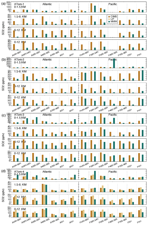
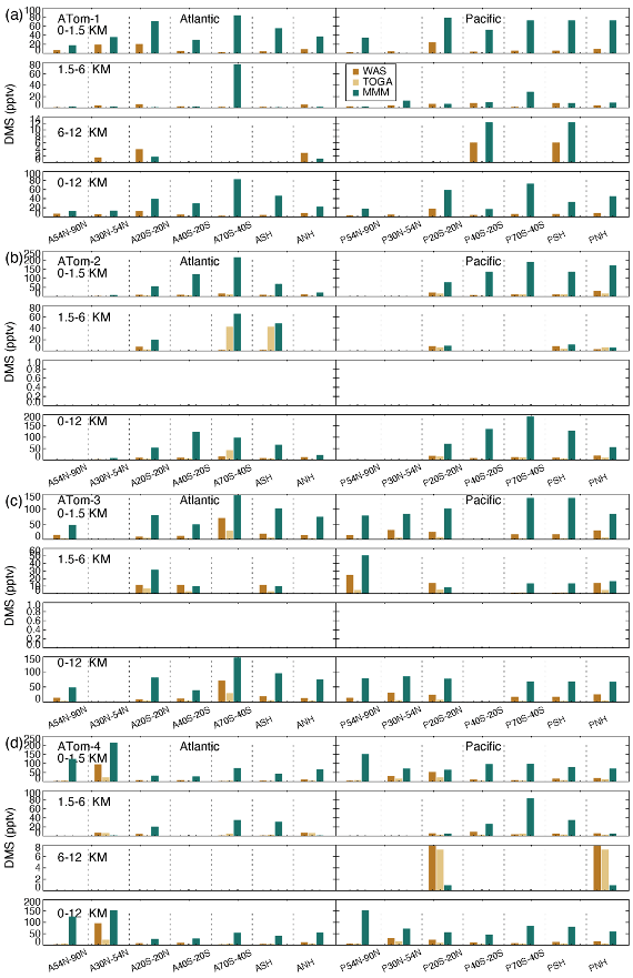
In order to analyze model performance on a regional and seasonal basis, Figs. 10–12 show histograms of SO₄, SO₂, and DMS concentrations as a function of altitude (rows) and latitudinal band (columns). Only the multi-model median is shown here to highlight any common problems in the models. Further details of each individual model are given in Figs. S9–S11 and discussed in the Supplement. Each model in this study has its bias at a specific time and location. With the information provided by Figs. S9–S11, modelers can further explore the simulation to identify potential causes of model anomalies.

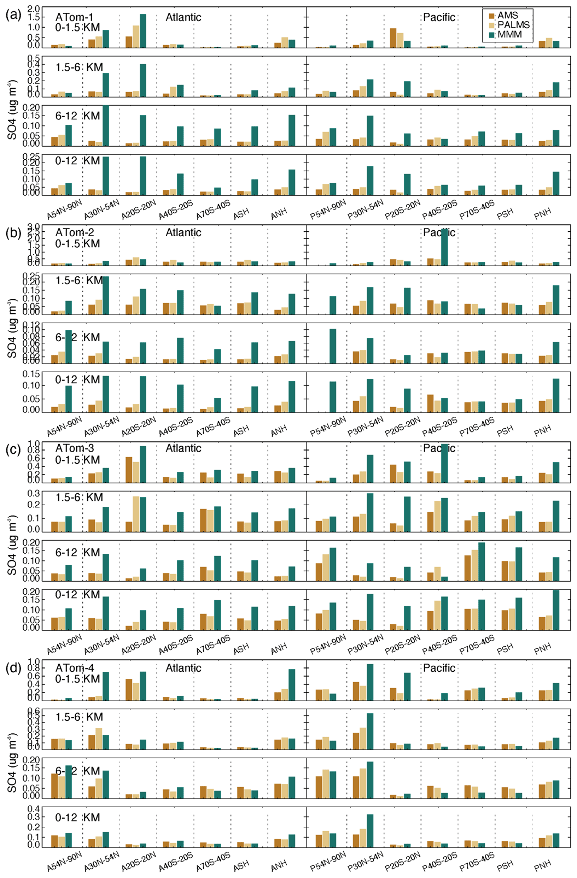
Figure 10 Median SO₄ concentrations from two measurements (AMS orange and PALMS yellow) and multi-model simulation (green) at seven latitudinal bands (including SH and NH) and four vertical layers (i.e., 0–1.5, 1.5–6, 6–12, and 0–12 km) over the Atlantic and Pacific oceans for four ATom deployments (a–d).

Figure 11 Similar to Fig. 10 but for SO₂.

Figure 12 Similar to Fig. 10 but for DMS.

High-SO₄-concentration regions vary across seasons (Fig. 10). In the free troposphere (i.e., 1.5–12 km), these regions cover the tropics to mid-latitudes in summer and winter (i.e., ATom-1 and ATom-2) and shift to mid- to high latitudes in spring and autumn (i.e., ATom-3 and ATom-4). The areas with the highest concentration appeared in the SH high latitudes during ATom-3 (SH spring) and the NH high latitudes during ATom-4 (NH spring). In the BL, the tropical atmospheric SO₄ concentration appears to be always elevated, and SO₄ concentration levels and SO₄ interregional variation are more pronounced in ATom-1 (NH summer). Among all ATom deployments, the performance of the model SO₄ simulation is best for ATom-4 and worst for ATom-1 (NH summer). Compared to observations, the model tends to simulate higher SO₄ concentrations in the free troposphere. Both observations and simulations show that the SO₄ over the Pacific is higher than that over the Atlantic during autumn in NH high latitudes (ATom-3) and spring in NH mid-latitudes (ATom-4). The differences between observations and simulations are generally larger in the Atlantic than in the Pacific, particularly in the SH. SO₄ concentration levels in simulations and observations can differ significantly in certain areas of each ATom period. Differences may be caused by the majority of models or a few individual models. For example, in summer and winter, the CAM-ATRAS model gave the highest estimates of atmospheric SO₄ in the oceanic BL, but the IMPACT and OsloCTM3 models gave the highest estimates of atmospheric SO₄ in the free troposphere (Fig. S9). All models except the GEOS model generally overestimate SO₄ in the atmosphere.

Atmospheric SO₂ (Fig. 11) is most abundant in the BL of the NH mid-latitude Pacific Ocean during ATom-1 (NH summer) and the tropical Pacific BL during ATom-3 (NH autumn), and this high-SO₂ region extends to the atmosphere above. Areas where free-tropospheric SO₂ concentrations are relatively large do not necessarily follow the example of the BL. For instance, the free troposphere appears to be more polluted than other regions in the NH Pacific during ATom-2 and in the SH mid-latitude Atlantic (A40S–20S) during ATom-4 but not in the BL, implying a potential source of SO₂ by horizontal transport. The interregional variation in SO₂ in the BL is much larger than in the free troposphere, from which local oceanic sources of SO₂ can be inferred. In terms of model–observation comparison, model-simulated SO₂ in the free troposphere is generally lower, which is opposite to the case of SO₄. A rapid SO₂ to SO₄ chemical conversion in models could be one of the reasons. Figure S10 further shows individual model SO₂ simulations. For example, the E3SM model gives significantly higher SO₂ compared with the measurements and other models in the BL (Fig. S10). Unlike the case of SO₄, all models tend to underestimate SO₂ in the free troposphere, with some exceptions, such as the GEOS model for winter in the mid- to high-latitude North Pacific (ATom-2) and the CAM-ATRAS and IMPACT models for autumn in the mid-latitude South Atlantic (ATom-4).

Surface DMS (Fig. 12) is generally higher in the tropics when the ocean is warm and in mid–high latitudes during springtime (e.g., ATom-3 SH spring and ATom-4 NH spring). A remarkable pattern of high model DMS values in the BL is revealed throughout the ATom cycle. This phenomenon also occurs in the free lower troposphere but not necessarily in the upper troposphere. The high model DMS in the BL can be attributed to (1) DMS emission that is too high, (2) DMS chemical loss that is too slow, and (3) DMS vertical transport from the BL to free troposphere that is too slow. Additional insight can be obtained by focusing on remote high latitudes, for example the SH high-latitude (40–70^∘ S) Pacific, where land source impacts are limited. Thus, the higher simulated SO₂ there in the BL in ATom-4 ruled out a chemical cause due to low DMS loss. The extremely high surface DMS is also not due to the slow vertical transport because simulated DMS is also high in the layers above the BL. A large model DMS emission is likely responsible for the simulated high surface DMS. The overestimation of a surface DMS multi-model median in Fig. 12 is clearly attributable to the contribution of all models shown in Fig. S11, with the models CAM-ATRAS and OsloCTM3 being more prominent.

4 Sulfur budget from AeroCom models

Budget analysis is a simple and basic method that has been widely used to document the underlying performance of a model. This analysis allows us to evaluate the AeroCom III sulfur simulations against previous AeroCom I and AeroCom II studies and serves as a record for future model evaluations. Table 4 summarizes the global sulfur budgets for emissions, wet and dry deposition, and chemistry from the five models. Clearly, the largest source of sulfur (∼ 70 Tg S yr⁻¹) is SO₂ emitted directly from anthropogenic (∼ 78 %), biomass burning (∼ 2 %), and volcanic sources (∼ 20 %). Biogenic DMS (∼ 15–30 Tg S) produced and outgassed from the decomposition of marine organic molecules provides the largest natural source of sulfur to the atmosphere. A small amount of SO₄ (< 3 %) is emitted directly from anthropogenic sources.

Table 4 Global sulfur budget in 2017.

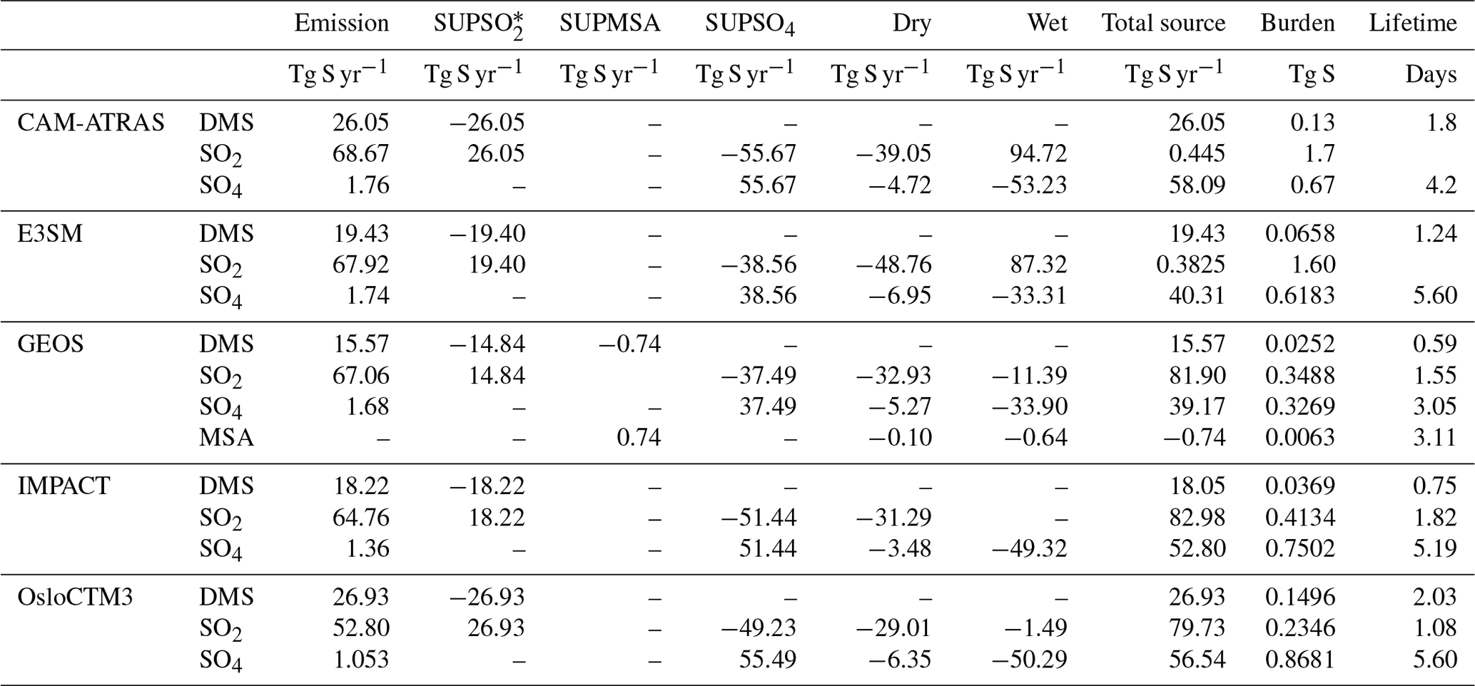
^* SUPSO₂: chemical production for SO₂.

Table 5 Global and annual sulfate multi-model mean and diversity from three AeroCom phases.

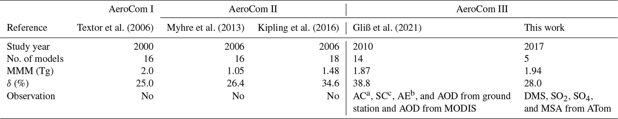
^a AC: aerosol absorption coefficients. ^b AE: Ångström exponent. ^c SC: aerosol scattering coefficients.

DMS is oxidized in the atmosphere by OH and NO₃ radicals to form SO₂ and MSA. This biological source of SO₂, along with SO₂ emitted directly from other sources, reacts with hydroxyl radicals (OH) in the gas phase and hydrogen peroxide (H₂O₂) and ozone (O₃) in the aqueous phase to produce sulfuric acid (H₂SO₄) and eventually sulfate particles, which play an important role in the formation of clouds over the oceans.

In the five models, DMS predicts the shortest global average lifetime (0.6–2.0 d), followed by SO₂ (1.1–1.8 d), and SO₄ the longest lifetime (3.1–5.6 d). Among them, GEOS has the lowest global burden and shortest lifetime for all sulfur species. The magnitudes of global burdens and lifetimes shown here support the model performance shown in Figs. 2–8. For example, models CAM-ATRAS and OsloCTM3 predicts the highest DMS emission, which is consistent with the highest DMS value (Figs. 4 and S11) and longest lifetime simulated by the two models.

The key budget items include DMS emission, SO₂ emission, sulfate source or total deposition (source and deposition are pretty much the same as expected), lifetime (inversely proportional to the loss rate), and total atmospheric mass load. From the multi-model mean and standard deviation, the diversity can be calculated. Figure 13 shows the global mean budget items in the percentage deviation of each model from the multi-model mean, following the same concept shown in Schulz et al. (2006) and Gliß et al. (2021). It reveals the processes causing model differences. For example, E3SM and GEOS have approximately the same SO₂ emissions and total sulfate sources, but the sulfate lifetime is much shorter in GEOS (implying faster removal rates and thus smaller sulfate burden), which is consistent with lower sulfate concentrations in GEOS than in E3SM. At the same time, the lower total sulfate source in E3SM is compensated by a longer lifetime compared to CAM-ATRAS, resulting in a comparable global burden of SO₄ in the two models.

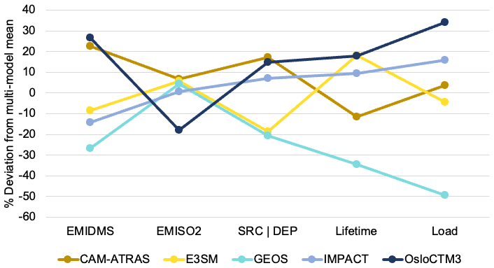
Figure 13 Deviation from multi-model mean for key budget items in sulfur study include DMS emission, SO₂ emission, sulfate source or total deposition, sulfate lifetime, and total sulfate atmospheric mass load.

It is worth pointing out that the much lower atmospheric SO₄ mass loading of the GEOS simulations is not necessarily related to the poor performance of the GEOS SO₄ simulations, as revealed by the model–measurement comparison in Figs. 2, 6, and S9. Although the multi-model mean (or median) often represents the best predictor in the modeling domain, common modeling problems or a model sample that is too small can compromise this effort.

To date, there have been no sulfur budget reports focusing on the vast ocean. However, previous AeroCom studies have reported global sulfate atmospheric loading and its diversity across multiple AeroCom models using monthly and global mean column loadings. Table 5 summarizes these studies, including their reported global and annual sulfate multi-model mean (MMM) and diversity (δ). δ is related to the standard deviation (SD) and is defined as δ= SD/MMM × 100 (%). The results of this work are lower than AeroCom I but higher than AeroCom II, which may be related to the different target years involved in these studies. One point to note is that the diversity δ of AeroCom III models has not reduced since AeroCom I, which was studied nearly 20 years ago.

5 Source origins for aerosol SO₄ along flight tracks and ocean basins

In this section, we perform an analysis of source attribution by tagging the sulfur source types using the GEOS model. This model is the only one that provides tagged data. Our goal is to understand the sources (anthropogenic, biological, volcanic) of sulfate aerosols in remote regions and how chemistry, transport, and removal processes determine the vertical distribution of sulfate aerosols across seasons and ocean locations.

Figure 14a presents a quantitative summary of the source attribution of aerosol SO₄ sampled along the ATom flight tracks. The analysis was performed over four seasons, spanning the troposphere and three vertical layers (i.e., marine boundary layer, free troposphere, and upper troposphere). Overall, anthropogenic emissions were the dominant source (40 %–60 % of the total) of simulated tropospheric SO₄ along the ATom flight tracks for almost all altitudes and seasons, followed by volcanic (18 %–32 %) and oceanic sources (16 %–32 %). Anthropogenic pollution prevailed over remote oceans most in spring and autumn (ATom-3 and ATom-4). The overall contributions from volcanic and oceanic sources are comparable during the ATom periods. Meanwhile, the ocean source contribution has an obvious seasonal variation which is most active during the SH summer (ATom-2), when marine biochemical activity in the vast Southern Ocean is the largest. Volcanos show the largest contribution in the NH summer of 2016 (ATom-1) during the four ATom deployments. Given the irregular character of eruptions, the volcanic contribution deserves further discussion below.

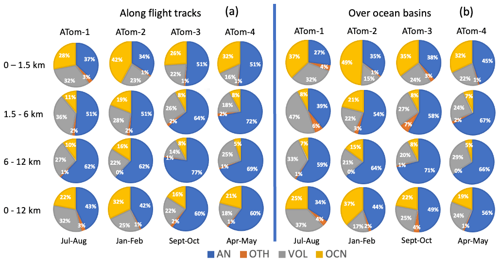
Figure 14 Source origins in percentage (%) for aerosol SO₄ along flight tracks (a) and for a wide oceanic area (b) based on the results from GEOS. Source origins are identified as anthropogenic (AN), volcanic (VOL), oceanic (OCN), and other sources (OTH). Ocean basins include the shaded region shown in Fig. 1.

In the vertical direction, SO₄ from anthropogenic emissions contributes more than 50 % to the free to upper troposphere. Even in the marine boundary layer, anthropogenic sources of SO₄ still account for the largest fraction, except in the SH summer (ATom-2) when oceanic source became dominant. The relative importance of volcanic and marine sources varies not only seasonally but also vertically. Oceanic sources understandably make up a significant fraction (26 %–42 %) of SO₄ in the boundary layer. In the free troposphere, their contribution drops off sharply, reflecting their local surface source characteristics. On the other hand, SO₄ from anthropogenic emissions (including shipping emissions) expands in the free troposphere, suggesting that the source originated from distant continental areas. Volcanic SO₄ remains nearly constant throughout the troposphere, making volcanoes the second largest source there. Meanwhile, the contribution of others (OTH including biomass burning) to remote ocean SO₄ is relatively small (< 3 %) and will not be discussed further in this study.

The sources of SO₄ discussed above are deduced from the location and timing of the ATom flight path. Conclusions about the total contribution of the ocean needs caution, as there may be representativeness issues using such narrow-band and instantaneous sampling. There might be a situation where, for example, volcanoes provide a very large signal but only account for a small measured area, and in most regions, volcanoes play a very minor role. Whereas oceanic sources in the marine boundary layer perhaps were the dominant source for a much wider region, the SO₄ concentration resulting from the DMS was overall a smaller amount compared to other sources near a volcanic or anthropogenic source. To address this representation issue, we perform one more analysis with the model data averaged over a wider oceanic region (the shaded area in Fig. 1) and over a longer period (i.e., monthly mean over ATom periods). Such source attributions are given in Fig. 14b.

Qualitative conclusions drawn from source attribution along the flight tracks generally apply to the ocean basin source attribution, albeit to a slightly different extent. This confirms that continental anthropogenic sources dominate tropospheric SO₄ even over oceans. There is a clear seasonal variation in the oceanic contribution, which is largest in austral summer (ATom-2) followed by boreal summer (ATom-1). Concerning volcanic sources, emissions from volcanoes are of two types. One type is the volcanic degassing emissions that tend to remain nearly constant throughout the year and are equivalent to about 20 % of global anthropogenic SO₂ emissions. This degassing emission ensures that volcanoes contribute more than 20 % to SO₄ over the oceans. The other type consists of the volcanic eruptions. Due to the irregularity of volcanic eruptions in terms of different eruption locations, magnitudes, and times, volcanic eruptions can cause severe fluctuations in SO₄ in the atmosphere. Compared with the source attribution along the flight trajectory, the volcanic contribution decreased over a larger spatial and temporal domain (i.e., ocean basin and monthly mean) in the NH winter of 2017 by 32 % (ATom-2) and increased in all of the other three seasons by 14 %–33 %, especially in the NH spring 2018 (ATom-4), when the massive Kilauea eruption in Hawaii began on 3 May 2018. Contrarily, the anthropogenic contribution increased in the NH winter (ATom-2) by 5 % and decreased in other seasons by 7 %–21 %.

6 Conclusions

This study investigates sulfur species in remote tropospheric regions at global and seasonal scales using airborne ATom measurements and AeroCom models. The goal is to understand the atmospheric sulfur cycle over the remote oceans, each model's behavior, and the spread of model simulations, as well as the model–observation discrepancies. Such an understanding and comparison with real observations are crucial to narrow down the uncertainty in model sulfur simulation. Even after decades of development, models are still struggling to accurately simulate sulfur distributions, with differences between models often exceeding an order of magnitude. On the other hand, the agreement between instruments is usually much better. Differences between modeled SO₄ are particularly large in the tropical upper troposphere, where deep convective transport allows a small portion of sulfur to reach the lower stratosphere where sulfate aerosols can persist for many years. Compared with observations, simulated SO₂ is generally low, while SO₄ is high. Modeled DMS values are typically an order of magnitude higher than observed DMS values near the surface, pointing to a need to revisit the DMS emission inventories and/or the biogeochemical modules used to predict DMS emissions. Our work also suggests investigating three other potential corresponding processes to improve sulfur simulation: whether the chemical conversion from SO₂ to SO₄ is too rapid, whether DMS-generated free-tropospheric SO₂ is too low, and whether the vertical transport of DMS and SO₂ from the BL to free troposphere is too low. This further investigation requires atmospheric oxidant fields and the ability to track SO₂ production and loss using tagged tracers.

We investigate source attribution of SO₄ over remote oceans seasonally and vertically. Sampled at the location and time of ATom measurements, anthropogenic emissions were the dominant source (40 %–60 % of the total) of simulated tropospheric SO₄ at almost all heights and seasons, followed by volcanic (18 %–32 %) and oceanic sources (16–32 %). These contributions changed to 34 %–56 %, 17 %–37 %, and 19 %–37 % when extended to the broad Pacific and Atlantic during the months of ATom deployment. This survey confirms that anthropogenic sources dominate tropospheric SO₄ even over oceans. Given that we find the DMS source to be overestimated in the models, the anthropogenic sources overall are a larger portion of the budget, and biogenic is likely smaller than volcanic. Volcanic degassing throughout the year contributes about 20 %, and this proportion is increased by explosive eruptions that vary in location and timing. The oceanic contribution has obvious seasonal variation, the largest being in the Southern Hemisphere summer, followed by the Northern Hemisphere summer.

It is understood that anthropogenic sulfur emissions currently offset a significant portion of greenhouse gas warming, but they are rapidly declining through emissions controls. As these anthropogenic emissions decrease, natural sources of sulfur, particularly bio-derived sulfur compounds discharged from the world's oceans, will increase their relative contribution. Therefore, more efforts are needed to understand the sulfur cycle in remote environments. On the other hand, our study is the first asserting that anthropogenic emissions remain a major source of sulfate aerosols generated over remote oceans during the ATom deployment periods, suggesting that any limitation of anthropogenic sulfur emissions would have modern global implications.

Even after 2 decades of development, the diversity of sulfate simulations from AeroCom I to AeroCom III has not decreased. However, accurate sulfate simulation in current climate models is crucial to reduce radiative forcing biases. More importantly, apart from the shortcomings of individual models, all modelers involved in this work should focus on the calculation of the air–sea exchange flux formula as it plays a key role in determining DMS emissions. To our knowledge, many other aerosol models employ similar formulas in air–sea flux calculations, so the findings here are applicable to them as well. Modelers also need to study DMS and SO₂ vertical transport as well as SO₄ wet deposition during long-distance transport, as model biases are greatest at high altitudes. One suggestion to modelers is that the use of online oxidant fields is insufficient to explain the model sulfate bias, as there was no systematic bias in the sulfate simulations between the models using interactive oxidants and the models using archival oxidants in this study. The complexity of chemistry deserves more attention.