An overview of the vertical structure of the atmospheric boundary layer in the central Arctic during MOSAiC

Observations collected during the Multidisciplinary drifting Observatory for the Study of Arctic Climate (MOSAiC) provide an annual cycle of the vertical thermodynamic and kinematic structure of the atmospheric boundary layer (ABL) in the central Arctic. A self-organizing map (SOM) analysis conducted using radiosonde observations shows a range in the Arctic ABL vertical structure from very shallow and stable, with a strong surface-based virtual potential temperature (θ_v) inversion, to deep and near neutral, capped by a weak elevated θ_v inversion. The patterns identified by the SOM allowed for the derivation of criteria to categorize stability within and just above the ABL, which revealed that the Arctic ABL during MOSAiC was stable and near neutral with similar frequencies, and there was always a θ_v inversion within the lowest 1 km, which usually had strong to moderate stability. In conjunction with observations from additional measurement platforms, including a 10 m meteorological tower, ceilometer, and microwave radiometer, the radiosonde observations and SOM analysis provide insight into the relationships between atmospheric vertical structure and stability, as well as a variety of atmospheric thermodynamic and kinematic features. A low-level jet was observed in 76 % of the radiosondes, with stronger winds and low-level jet (LLJ) core located more closely to the ABL corresponding with weaker stability. Wind shear within the ABL was found to decrease, and friction velocity was found to increase, with decreasing ABL stability. Clouds were observed within the 30 min preceding the radiosonde launch 64 % of the time. These were typically low clouds, corresponding to weaker stability, where high clouds or no clouds largely coincided with a stable ABL.

1 Introduction

The atmospheric boundary layer (ABL) is the turbulent lowest part of the atmosphere that is directly influenced by the earth's surface (Stull, 1988; Marsik et al., 1995). Its structure dictates the transfer of energy, moisture, and momentum between the Earth's surface and the overlying atmosphere (Brooks et al., 2017). Understanding the vertical structure of the ABL is particularly important for the central Arctic, where the ABL serves as a shallow interface between a thinning and retreating sea ice surface (Stroeve and Notz, 2018; Ding et al., 2017; Serreze and Barry, 2011) and a rapidly warming atmosphere (Rantanen et al., 2022; Serreze and Francis, 2006). Shortcomings in numerical prediction tools at high latitudes (Randriamampianina et al., 2021; Docquier and Koenigk, 2021) can be partly attributed to imperfect representation of the Arctic ABL, particularly its thermodynamic and kinematic structure (de Boer et al., 2014; Wesslén et al., 2014; Birch et al., 2012; Tjernström et al., 2008). Thus, it is important to continue building upon what is already known about the Arctic ABL structure with new datasets when available so that Arctic changes under continued anthropogenic warming and effects on global climate can better be predicted.

Previous studies have revealed that the Arctic atmosphere over sea ice is typically either stable or near neutral (Tjernström and Graversen, 2009; Persson et al., 2002; Esau and Sorokina, 2010), while instability is rare or confined to the lowest few meters (Brooks et al., 2017; Tjernström et al., 2004; Persson et al., 2002). In the case of a near-neutral ABL, there is almost always an elevated capping potential temperature (θ) inversion (Kayser et al., 2017), typically with base height around 200–300 m, extending up to 1–2 km (Tjernström and Graversen, 2009). Surface-based and low-level θ inversions have been shown to contribute to Arctic amplification (Serreze and Francis, 2006; Serreze and Barry, 2011; Bintanja et al., 2011; Lesins et al., 2012; Gilson et al., 2018; Previdi et al., 2021) by dynamically decoupling the surface from the free atmosphere so that lower-atmospheric warming related to increased surface-to-air (or decreased air-to-surface) heat fluxes cannot easily spread through the troposphere and that warming is concentrated near the surface (Lesins et al., 2012). These θ inversions often correlate to a moisture inversion (increasing mixing ratio with height) at the same height, with strength proportional to that of the θ inversion (Naakka et al., 2018; Devasthale et al., 2011; Nygård et al., 2014; Cohen et al., 2017). In the Arctic, the near-surface climate and meridional transport support these moisture inversions (Devasthale et al., 2011), which are important for cloud formation and maintenance (Naakka et al., 2018; Cohen et al., 2017).

Stable conditions are common in Arctic winter (Walden et al., 2017; Tjernström and Graversen, 2009) due to persistent longwave cooling in the absence of solar radiation (Brooks et al., 2017; Kayser et al., 2017; Cohen et al., 2017) and extended periods of clear skies or thin high clouds (Tjernström and Graversen, 2009), attributable to the lack of open water evaporation. Shallow, stable ABL conditions in summer commonly occur due to the advection of warm moist air into the central Arctic (Tjernström et al., 2019; Tjernström, 2005; Cheng-Ying et al., 2011), especially towards the beginning of an advection event or close to the ice edge (Sotiropoulou et al., 2016; Tjernström et al., 2019).

Near-neutral or weakly stable conditions can occur in the presence of stratiform clouds (Intrieri et al., 2002a; Tjernstrom, 2007; Curry and Ebert, 1992; Liu and Key, 2016; Shupe et al., 2011; Tjernström, 2005; Tjernström et al., 2012; Wang and Key, 2005; Zygmuntowska et al., 2012). Increased near-surface temperatures associated with enhanced downwelling longwave radiation caused by cloud cover can erode the surface inversion (Tjernström et al., 2019), which is sometimes supplemented by downward mixing from the cloud itself (forced by cloud-top radiative cooling) (Morrison et al., 2012). This is common in Arctic summer (Walden et al., 2017) when ample moisture is advected north either into the Arctic or from the broader ice-free areas across the pan-Arctic region. (Sotiropoulou et al., 2016; Tjernström et al., 2019). Intermittent instances of low stratocumulus clouds in winter can also force a shallow well-mixed ABL (Kayser et al., 2017; Morrison et al., 2012; Tjernström and Graversen, 2009; Persson et al., 2002). Such clouds are common during stormy conditions (Brooks et al., 2017; Persson et al., 2002) such as Arctic cyclones, which have a greater impact on weakening ABL stability during winter than during other seasons (Kayser et al., 2017; Walden et al., 2017; Cohen et al., 2017). The ABL is often decoupled from the cloud layer by a shallow stable layer such that turbulence is not exchanged between the cloud and the surface (Curry, 1986; Sedlar and Shupe, 2014; Sedlar et al., 2012; Shupe et al., 2013; Sotiropoulou et al., 2014). Clouds containing liquid water have a warming influence on the surface most of the year when compared to clear-sky conditions (Brooks et al., 2017; Shupe and Intrieri, 2004). Previous cloud observations in the central Arctic revealed an annual average occurrence of 85 % (dominated by low clouds), with the monthly highest and lowest occurrences in September and February respectively (Intrieri et al., 2002b).

Another common feature of the Arctic atmosphere which contributes to the weakening of ABL stability is a low-level jet (LLJ), which is a local maximum in the wind speed profile below 1.5 km (Tuononen et al., 2015). Due to enhanced wind shear and subsequent turbulent kinetic energy production, an LLJ can contribute to mechanically generated turbulence below the jet core (Egerer et al., 2023; Banta, 2008; Mahrt, 2002; Mäkiranta et al., 2011). Previous studies in the central Arctic have reported a range in LLJ frequency. Jakobson et al. (2013) found an LLJ frequency of 46 % during spring and summer. Tian et al. (2020) and ReVelle and Nilsson (2008) found an annual LLJ frequency of 60 %–80 %, with a higher frequency of LLJs over the pack ice (72 %) versus in the marginal ice zone (66 %). A study conducted using some of the same measurements as this paper found LLJs to be present more than 40 % of the time in the central Arctic (Lopez-Garcia et al., 2022). Model studies of central Arctic LLJs have documented a lower frequency, of 20 %–25 % (Tuononen et al., 2015).

While much has already been discovered about the central Arctic lower-atmospheric structure, most field campaigns have occurred during the summer (e.g., the Arctic Ocean Experiment 2001 (AOE-2001; Tjernström, 2005), the Arctic Summer Cloud Ocean Study (ASCOS; Tjernström et al., 2014), and the Arctic Clouds in Summer Experiment (ACSE; Tjernström et al., 2015)) or in coastal regions (e.g., the Profiling at Oliktok Point to Enhance Year of Polar Prediction Experiments (POPEYE; de Boer et al., 2019) and the Summertime Aerosol across the North Slope of Alaska Field Campaign (Pratt et al., 2018)). The only previous campaign to cover an entire year over Arctic sea ice (the Surface Heat Budget of the Arctic Ocean (SHEBA) project; Uttal et al., 2002) occurred over 20 years ago, since which there have been widespread changes in the Arctic climate system. Additionally, there in inconsistency in the frequency of stable versus near-neutral conditions across previous literature. For example, Esau and Sorokina (2010) claim that the central Arctic ABL is stable 70 %–90 % of the time based on lower-resolution observational and reanalysis data, while Tjernström and Graversen (2009) found stable and near-neutral conditions to occur with similar frequencies based on higher-resolution observations from SHEBA in the Beaufort gyre. Thus, there is much to be gained by analysis of more recent data, such as those from the Multidisciplinary drifting Observatory for the Study of Arctic Climate (MOSAiC; Shupe et al., 2020), which observed the central Arctic following one ice floe for a full year from September 2019 to October 2020. As such, this study utilizes observations from MOSAiC to analyze the lower atmosphere, focusing on vertical structure and stability and characteristics of wind and atmospheric moisture corresponding to this varying vertical structure and stability, to provide a summary of the aforementioned conditions and relationships over a full annual cycle. A complementary paper (Jozef et al., 2023b) explores the role of kinematic (e.g., wind characteristics forced by synoptic setting) and thermodynamic (e.g., surface radiation budget forced by clouds) processes that contribute to, and are modified by, vertical structure and stability conditions, so such details are not heavily discussed in the current paper.

The questions guiding this study are as follows: what was the range of lower-atmospheric thermodynamic vertical structure and stability observed during MOSAiC and how did this vary by season? How does thermodynamic vertical structure and stability correspond with features related to wind and atmospheric moisture? How do the characteristics of the ABL (depth, wind shear, and turbulence) vary with stability?

To determine thermodynamic and kinematic vertical structure and stability, we primarily use profile data from radiosondes launched at least four times per day throughout the MOSAiC year, supplemented with continuous observations of the near-surface meteorological state and atmospheric clouds and moisture from additional measurement platforms. A self-organizing map (SOM) analysis (which objectively identifies a user-selected number of patterns present in a training dataset) was conducted with the radiosonde profiles to reveal the range of vertical structures observed during MOSAiC (differentiated by stability within the ABL and the height and strength of a capping inversion), their relative frequencies, and their correlation to wind and moisture features during the MOSAiC year. The SOM results were also used to develop criteria to define stability regimes characterized by stability both within and above the ABL such that features related to stability can be analyzed both in the context of the SOM patterns, as well as a more simplified grouping of observations by stability. Through the use of these new methods (i.e., the SOM analysis and detailed stability regime classification), the results provide further constraints on the vertical structure and features of the Arctic lower atmosphere that may be helpful to improve parameterizations of the central Arctic in weather and climate models.

2 Methods

2.1 Observational data from MOSAiC

Data used in this study were collected during MOSAiC, a year-long icebreaker-based expedition lasting from September 2019 through October 2020, in which the research vessel Polarstern (Alfred-Wegener-Institut Helmholtz-Zentrum für Polar- und Meeresforschung, 2017) was frozen into the central Arctic Ocean sea ice pack and was set to drift passively across the central Arctic for the entire year. During the MOSAiC year, many measurements were taken to observe the atmosphere (Shupe et al., 2022), sea ice (Nicolaus et al., 2022), and ocean (Rabe et al., 2022), resulting in the most comprehensive set of observations of the central Arctic climate system to date. These measurements span all seasons, as well as those both far from and close to the sea ice edge, as the Polarstern essentially followed one ice floe for its annual life cycle (only relocating to a new ice floe for the final 2 months of the expedition).

For this study, we primarily use profile data from the balloon-borne Vaisala RS41 radiosondes, which were launched from the helicopter deck of the Polarstern (∼ 12 m a.s.l.) at least four times per day (every 6 h), typically at 05:00, 11:00, 17:00, and 23:00 UTC (Maturilli et al., 2021). We use the level 2 radiosonde product (Maturilli et al., 2021) for this analysis, as the level 2 Vaisala-processed product is found to be more reliable in the lower troposphere than the level 3 Global Climate Observing System Reference Upper-Air Network (GRUAN)-processed product (Maturilli et al., 2022). Figure 1 shows the location of each radiosonde launch throughout the MOSAiC year. From the radiosondes, we utilize measurements of temperature, pressure, relative humidity, and wind speed and direction. The radiosondes ascend at a rate of approximately 5 m s⁻¹, sampling with a frequency of 1 Hz, which results in measurements about every 5 m throughout the ascent. Instrument specifications and uncertainties for the radiosonde variables are provided in the manufacturer data sheet for the Vaisala Radiosonde RS41-SGP (2017) and are summarized in Table 1. It is recognized that the true uncertainties in the wind speed and direction are likely to be greater than those provided in the data sheet; however for the following reasons, we find the original winds provided in Maturilli et al. (2021) to be sufficiently reliable for the current study. First, we determined that our results changed minimally when additional vertical averaging was applied to the winds (beyond the filtering already applied by Vaisala during their data processing), and thus noise in the observations does not bias the results. Second, when comparing radiosonde wind speeds to those measured by the DataHawk2 uncrewed aircraft system which observed the atmosphere during MOSAiC between 5 m and 1 km, Hamilton et al. (2022) found a difference of less than 1 m s⁻¹ based on the 95 % confidence intervals of observations from both platforms. Nonetheless, caution should be taken with the interpretation of radiosonde wind speeds in the lowest 100 m.

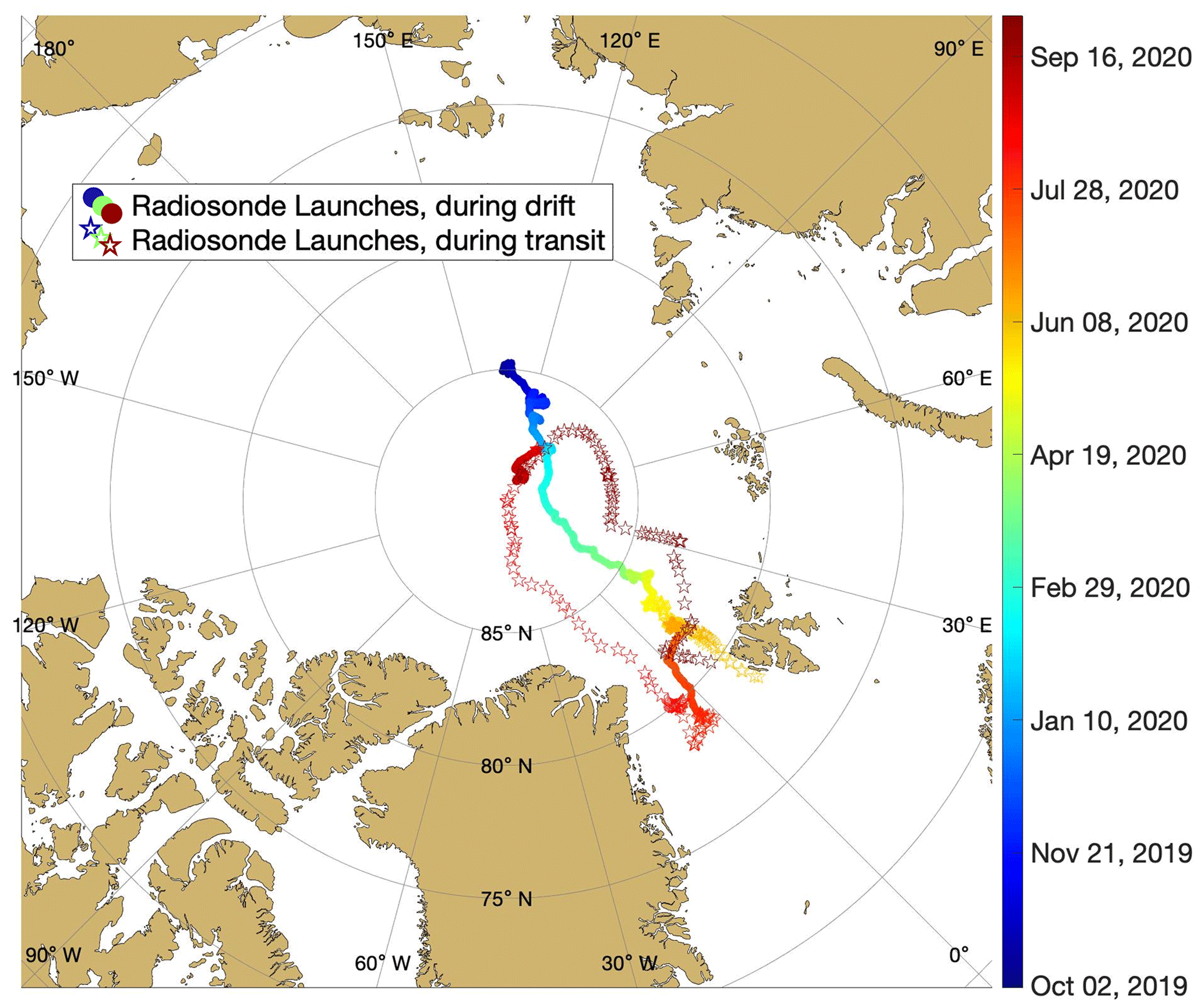
Figure 1 Map of the central Arctic showing the location of each radiosonde launch, color coded by date. Circular symbols indicate when the Polarstern was passively drifting, and star symbols indicate when the Polarstern was traveling under its own power.

Table 1 Instrument name and uncertainty for each variable used in this study, as provided by the manufacturer (real uncertainties may differ from those listed).

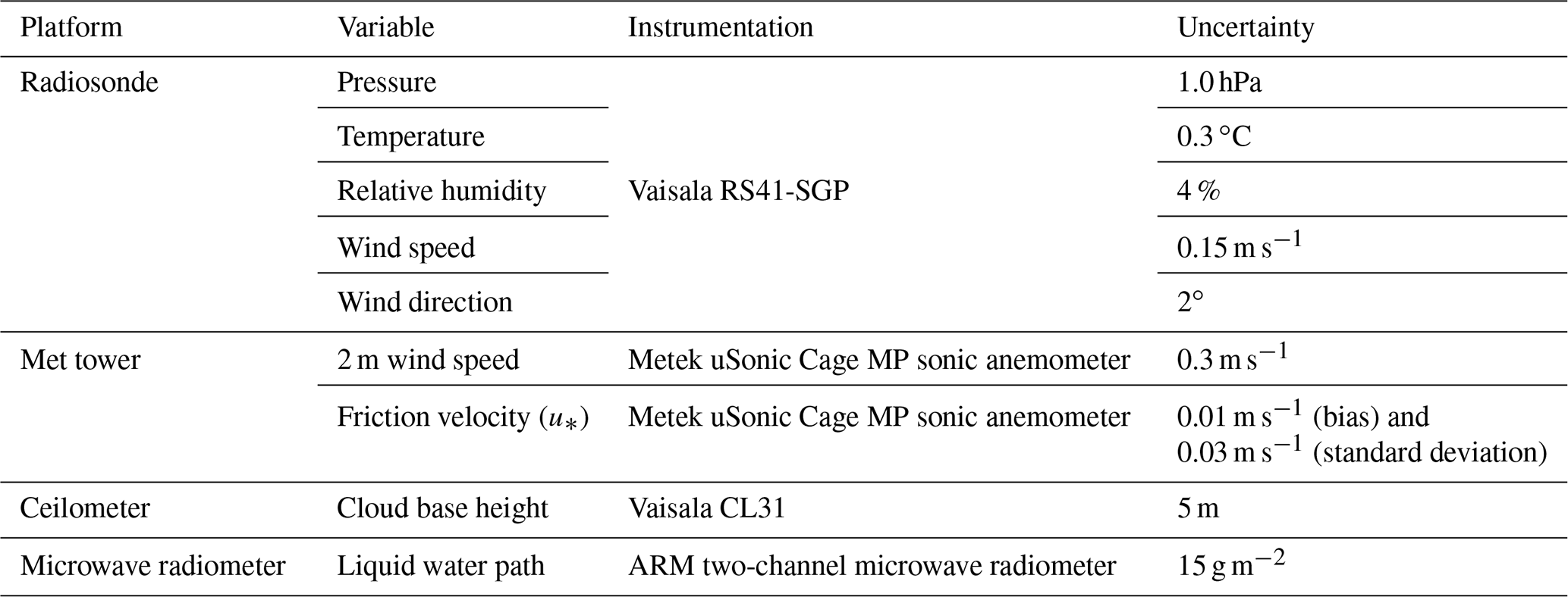
In addition to the profile data provided by the radiosondes, we utilize observations from a few other measurement platforms which add to the overall description of the ABL at the time of each radiosonde launch. Atmospheric observations of wind speed at 2 m above the surface, as well as friction velocity (a measure of the vertical fluxes of zonal and meridional horizontal momentum, suggesting the magnitude of mechanically generated turbulence; u_∗) measured at 10 m, come from a 10 m meteorological tower (hereafter called the met tower) located on the sea ice near the Polarstern (Cox et al., 2023a, b). These measurements provide information about near-surface turbulence at the time of each radiosonde launch. Derivation of u_∗ through standard eddy-covariance methodology and corresponding uncertainties follow Persson et al. (2002).

Information on cloud cover comes from a Vaisala CL31 ceilometer (ARM User Facility, 2019a), which derives cloud base height (CBH) from measured atmospheric backscatter and allows us to determine the altitude and frequency of clouds at and before radiosonde launch. CBH derivation and uncertainty are discussed in Morris (2016). Additionally, liquid water path (LWP) comes from the MWRRET Value-added Product (ARM User Facility, 2019b) which derives LWP from ARM two-channel microwave-radiometer-measured brightness temperatures. LWP derivation and uncertainty are discussed in Turner et al. (2017) and Cadeddu et al. (2013) respectively. Both the ceilometer and microwave radiometer were located on the P-deck of the Polarstern (depicted in Fig. 3 of Shupe et al., 2022), which is approximately 20 m a.s.l., and could occasionally be above a layer of shallow fog. Table 1 lists the instrument name and uncertainty for each of the observational variables used in this study.

2.2 Deriving quantities from observational data

Before the radiosonde profiles were analyzed, measurements were corrected to account for the local “heat island” resulting from the presence of the Polarstern. This local source of heat resulted in the frequent occurrence of elevated temperatures near the launch point, resulting in inconsistencies in the observed temperatures in the lowermost part of the atmosphere. This phenomenon can be recognized by an artificial temperature structure indicative of a convective layer in the lowest radiosonde measurements, which we know is unlikely (Tjernström et al., 2004; Brooks et al., 2017). Thus, if this “convective layer” was present, then the lowest radiosonde measurements were visually compared to measurements from the met tower to confirm whether the radiosonde measurements were indeed incorrect (e.g., if the lowest few radiosonde measurements were notably warmer then the tower measurement at 10 m). The first credible value of the radiosonde measurements was then taken to be the point at which the tower measurements extrapolated upward would line up with the observed radiosonde measurement or, in the case of a temperature offset between the tower and radiosonde, would have approximately the same slope. All data at the altitudes below this first credible value were removed. This helps in also removing faulty wind measurements that occur as a result of flow distortion around the ship (Berry et al., 2001).

An additional disruption of the radiosonde measurements sometimes occurred because of the passage of the balloon through the ship's exhaust plume. When it was unambiguous that the radiosonde passed through the ship's plume (evident by a sharp increase and subsequent decrease in temperature, typically by ∼ 0.5–1 ^∘C over a vertical distance of ∼ 10–30 m, identified visually), these values were replaced by values resulting from interpolation between the closest credible values above and below the anomalous measurements, which were identified as the last point just before the increase and the first point just after the decrease in temperature values, to acquire a continuous profile of reliable temperatures. Lastly, we determined that 92 % of profiles have credible measurements as low as 35 m a.g.l. To allow for a consistent bottom height for our analysis, we only considered profiles in which there is a good measurement at 35 m and did not consider any data below 35 m. This altitude is a compromise between removing too much low-altitude data or removing too many radiosonde profiles from analysis. After removing all profiles in which there is not trustworthy data as low as 35 m, we retain 1377 MOSAiC radiosonde profiles for analysis. The 132 profiles which were removed from analysis are dispersed throughout the year, but many of them were observations from early October, mid-April (an intensive period when radiosondes were being launched every 3 h), or mid-September.

ABL height from each radiosonde profile was determined using a bulk Richardson number-based (Ri_b-based) approach in which the top of the ABL was identified as the first altitude at which Ri_b exceeds a critical value of 0.5 and remains above the critical value for at least 20 consecutive meters (Jozef et al., 2022). Ri_b profiles were created by calculating Ri_b across 30 m intervals in steps of 5 m, rather than using the ground as the reference level, in order to isolate the local likelihood of turbulence rather than that over the full depth from the surface (Jozef et al., 2022). These criteria typically identify the ABL height as the bottom of the elevated virtual potential temperature (θ_v) inversion (or the bottom of the layer of enhanced θ_v inversion strength) for moderately stable to near-neutral conditions, as well as at the top of the most stable layer for conditions with a strong surface-based θ_v inversion. Further details on the methodology for calculating the Ri_b profile used to identify ABL height, as well as justification for the use of 0.5 as a critical value (rather than the more traditional value of 0.25), are described in Jozef et al. (2022).

LLJs were identified from each radiosonde, where there was a maximum in the wind speed that was at least 2 m s⁻¹ greater than the wind speed minimum above (Stull, 1988). As described in Tuononen et al. (2015), only situations in which both the wind speed maximum (the LLJ core) and the minimum above the core were both below 1.5 km were identified as LLJs. When there were multiple maxima, we only considered the lowest one, and a maximum was only considered an LLJ when it was at least 2 m s⁻¹ greater than the next local minimum above the LLJ or the value at 1.5 km (if no local minimum above the maximum), as in Tuononen et al. (2015). If an LLJ was found, we identified the LLJ core altitude as the altitude of the maximum in the wind speed and the LLJ core speed as the wind speed at that altitude (Jakobson et al., 2013). Further details are presented in Jozef et al. (2023a). Vertical averaging was not applied to the wind speed profiles before identification of LLJs in the current study, as there is no significant difference in LLJ frequency at the 95 % confidence level when applying a 30 m running mean, and thus vertical averaging was deemed unnecessary for the improvement of result accuracy. Our analysis differs from that by Lopez-Garcia et al. (2022) as they only considered LLJs in which the jet core speed was at least 25 % greater than the wind speed minimum above the jet core, whereas we do not include this criterion, and thus our analysis also includes LLJs which occur in ubiquitously high-wind-speed environments (e.g., a wind speed maximum of 20 m s⁻¹ would be 2 m s⁻¹ faster, but not 25 % faster, than a wind speed minimum of 17 m s⁻¹ above).

Cloud and moisture characteristics associated with each radiosonde were identified using measurements within the 30 min preceding the radiosonde launch. Thus, CBH and LWP were taken as the average within that 30 min interval. We use this 30 min interval, as this is a long enough time for the presence of the cloud and atmospheric moisture to impact atmospheric stability and structure close to the surface. Any other point measurements associated with each radiosonde (2 m wind speed and u_∗) were calculated as the average over a period of 5 min before to 5 min after the radiosonde launch, as described in Jozef et al. (2023a).

2.3 Self-organizing map analysis

The SOM analysis uses an unsupervised neural network algorithm to objectively identify a user-specified number of patterns in a training dataset (Cassano et al., 2015; Kohonen, 2001). In doing so, this analysis projects high-dimensional input data onto a low-dimensional space as a grid of SOM-identified patterns (Liu and Weisburg, 2011) and provides a compact way to visualize the range of conditions present in the training data. The grid of SOM-identified patterns is referred to as a SOM or simply a map. Atmospheric applications of SOMs have previously been used to determine ranges of synoptic patterns (Nygård et al., 2021; Cassano et al., 2015; Sheridan and Lee, 2011; Skific et al., 2009; Cassano et al., 2006; Hewitson and Crane, 2002); identify large-scale circulation anomalies associated with extreme weather events (Cavazos, 2000); and classify cloud (Ambriose et al., 2000), climate zone (Malmgren and Winter, 1999), precipitation (Crane and Hewitson, 2003), and ice core data (Reusch et al., 2005), to name a few. Most similar to the current study, SOMs have previously been used to identify the range of ABL structures in Antarctica from both tower (Nigro et al., 2017; Cassano et al., 2016) and radiosonde (Dice and Cassano, 2022) data. Here, the SOM analysis is applied to radiosonde profiles of θ_v gradient to identify vertical structure and stability in the lowest 1 km of the atmosphere over the Arctic ice pack during MOSAiC.

A SOM is created by randomly initializing patterns from the input data space and comparing the training data to these patterns. Each sample in the input data is presented to the SOM and compared to all patterns in the initial map. The pattern to which the input data sample is most similar is known as the “winning” pattern, and this pattern and adjacent neighboring patterns are modified to reduce the squared difference between it and the input data sample. This process continues for all samples in the training data (Liu and Weisburg, 2011; Cassano et al., 2006) and is repeated thousands of times for the entire training dataset until the squared differences between the SOM-identified patterns and the training data have been minimized. Further details on how a SOM is trained are given in the papers cited above. Here we use the SOM-PAK software (http://www.cis.hut.fi/research/som-research, last access: 24 January 2022; Kohonen et al., 1996) to train the SOM presented below.

A critical decision when using SOMs is the number of patterns to be identified by the SOM training, and this depends on the intended application and size of the training dataset (Cassano et al., 2006). A greater number of patterns will produce a broader range of structures with more subtle differences between them, and fewer patterns will result in larger variability between and within the patterns. Regardless of the number of patterns identified in the SOM, the SOM provides a smoothly varying, continuous depiction of the range of conditions present in the training data. The output from the SOM training is a two-dimensional array of patterns which are representative of the range of conditions present in the training data (Cassano et al., 2006). The SOM is organized such that the patterns being most similar are located adjacently, and conversely the most different patterns are on opposite sides of the SOM (Dice and Cassano, 2022; Cassano et al., 2016; Liu and Weisburg, 2011). Each sample in the training data is mapped to the resulting SOM pattern with which it has the smallest squared difference resulting in a list of samples for each SOM-identified pattern. This list of data samples can then be used to calculate the frequency of each SOM pattern and for additional analyses (Dice and Cassano, 2022).

In this study, a 30-pattern SOM was used to describe the range of lower-atmospheric stability profiles, defined by the θ_v gradient ($\mathrm{d}{\mathit{\theta }}_{\mathrm{v}}/\mathrm{d}z$), present in the 1377 MOSAiC radiosonde profiles. Before settling on the 6 × 5 (30-pattern) SOM, we tested SOMs with sizes and orientations of 5 × 4 (20 patterns) to 7 × 5 (35 patterns). When using 20 patterns, the range in strength of near-surface stability and the varying depths of a weakly stable or near-neutral layer were not fully evident. To fully understand the range of vertical structures in the Arctic, highlighting these differences is important, so the inclusion of additional SOM patterns was necessary. However, with 35 patterns, we found that no additional details were introduced beyond what was shown with 30 patterns. Thus, we determined that 30 patterns is the smallest number to sufficiently describe the range of lower-atmospheric stability during MOSAiC, retaining fundamental features of vertical structure (e.g., varying height and strength of the θ_v inversion). We also tested the SOM trained with the θ_v profiles rather than the gradient (in the form of the θ_v difference with respect to that at 1 km to remove seasonal temperature dependence) but found that the range in height and strength of the θ_v inversion and the differentiation between a weakly stable or near-neutral layer below a θ_v inversion were not as evident.

The profiles of $\mathrm{d}{\mathit{\theta }}_{\mathrm{v}}/\mathrm{d}z$ used to train the SOM were derived from radiosonde observations that were first interpolated to a consistent vertical grid of 5 m spacing between 35 m and 1 km (temperature and relative humidity were linearly interpolated, and pressure was interpolated with the hypsometric equation). The maximum altitude of 1 km was chosen because it includes the full depth of the ABL in every case and also allows for diagnosing stability immediately above the ABL. Then, θ_v was calculated at 5 m intervals using the interpolated measurements. Finally, profiles of $\mathrm{d}{\mathit{\theta }}_{\mathrm{v}}/\mathrm{d}z$ (in K (100 m)⁻¹) were calculated as the change in θ_v between adjacent data points, resulting in $\mathrm{d}{\mathit{\theta }}_{\mathrm{v}}/\mathrm{d}z$ values at 37.5, 42.5, 47.5 m, and so on, with the last value being at 997.5 m. Training the SOM with $\mathrm{d}{\mathit{\theta }}_{\mathrm{v}}/\mathrm{d}z$ profiles resulted in an array of patterns differentiated by the strength and height of the θ_v inversion. As such, observations with similar strength θ_v inversions which occurred at different heights and observations with similar heights of the θ_v inversion but different strengths were separated into different SOM-identified patterns.

The 30-pattern SOM of $\mathrm{d}{\mathit{\theta }}_{\mathrm{v}}/\mathrm{d}z$ and the spread in observations mapping to a given SOM pattern are provided in Supplement Fig. S1. However, a more tangible demonstration of the range of vertical structures present during MOSAiC is shown in Fig. 2 with the mean profiles of $\mathrm{d}{\mathit{\theta }}_{\mathrm{v}}/\mathrm{d}z$ and θ_v anomaly (where “anomaly” refers to the value at a given altitude minus the value at 1 km) for all radiosondes mapped to a given pattern. The full range of vertical structures revealed by the SOM was used to develop a set of criteria for classifying stability of any given observation that distills the details of the SOM to the most critical factors of stability within and above the ABL, which will be discussed in Sect. 2.4. Additional details included in Fig. 2 will be discussed later in the paper.

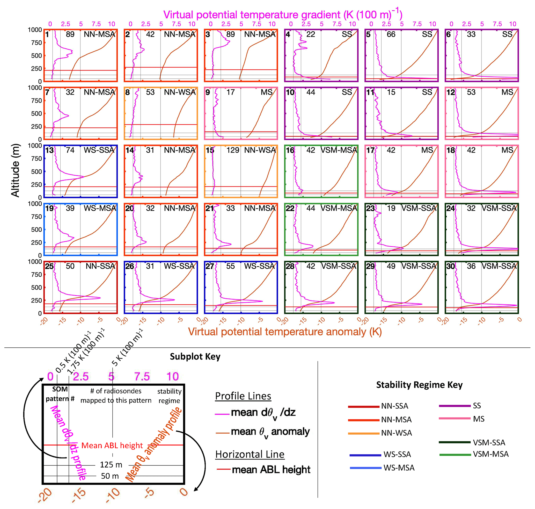
Figure 2 Mean virtual potential temperature (θ_v) anomaly profile (orange line, bottom x axis), mean virtual potential temperature gradient profile ($\mathrm{d}{\mathit{\theta }}_{\mathrm{v}}/\mathrm{d}z$; magenta line, top x axis), and mean ABL height (horizontal red line) for all radiosonde profiles mapped to each SOM pattern. Horizontal black lines at 50 and 125 m a.g.l. and vertical black lines at 0.5, 1.75, and 5 K (100 m)⁻¹ used to classify stability regime are included. The bold number in the upper left-hand corner of each subplot is the number of that SOM pattern (1 through 30), the number in the upper center of each subplot is the number of radiosonde profiles which map to that pattern, and the letters in the upper right-hand corner of each subplot indicate that pattern's stability regime (see “subplot key”). Stability regime is also indicated by the color of the border for each subplot, following the colors given in the “stability regime key”.

2.4 Stability regime analysis

A total of 12 stability regimes have been defined based on stability within the ABL (hereafter referred to as “near-surface” stability) as well as the strength of the capping θ_v inversion located between the top of the ABL and 1 km (hereafter referred to as stability “aloft”; Table 2). These stability regime definitions are based on the range of profiles seen in the SOM (Fig. 2). The SOM made the development of these stability regime criteria possible, as it revealed a manageable number of physically meaningful patterns representative of the entire training dataset such that important variations between profile θ_v structures could be discerned. Based on these SOM results, stability regime criteria could be developed that were applicable to any θ_v profile and thus were applied to each SOM pattern (using the average of all radiosonde profiles mapped to a given SOM pattern), as well as to individual radiosonde profiles. The stability regime definitions were developed alongside a similar SOM-based analysis of ABL profiles in Antarctica (Dice et al., 2023). An iterative process was conducted by visually inspecting the MOSAiC and Antarctic SOMs to identify groupings within each SOM which appeared to be substantially different from other groupings in that SOM, based on the near-surface and aloft stability. Then, thresholds (based on prior literature where possible) were determined to differentiate each grouping that made sense for the MOSAiC SOM and all the Antarctic SOMs. This process was completed considering both Arctic and Antarctic SOMs to support the robustness of these methods for classifying stability in either polar region and to reduce subjectiveness. Further details about the determination of thresholds are provided below.

Table 2 Thresholds used to differentiate between stability regime, where the various near-surface regimes are SS (strongly stable), MS (moderately stable), VSM (very shallow mixed), WS (weakly stable), and NN (near neutral) and the various stabilities aloft are -SSA (strongly stable aloft), -MSA (moderately stable aloft), and -WSA (weakly stable aloft).

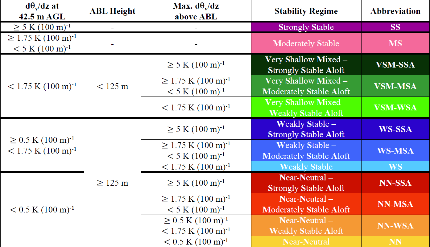
Before identifying stability regime, we must smooth some of the noise in the original $\mathrm{d}{\mathit{\theta }}_{\mathrm{v}}/\mathrm{d}z$ profiles. Since the stability criteria in part depend on stability within the ABL and some observations have an ABL height as low as 50 m, we first include a measurement of $\mathrm{d}{\mathit{\theta }}_{\mathrm{v}}/\mathrm{d}z$ at 42.5 m (this determines the near-surface stability), calculated across a 15 m interval between 35 m (lowest point of the profile) and 50 m. For values at and above 50 m, $\mathrm{d}{\mathit{\theta }}_{\mathrm{v}}/\mathrm{d}z$ is calculated across 30 m intervals in steps of 5 m and attributed to the center altitude of Δz (i.e., 35–65, 40–70, 45–75 m, and so on), resulting in a $\mathrm{d}{\mathit{\theta }}_{\mathrm{v}}/\mathrm{d}z$ profile with values at 42.5, 50, 55, 60 m a.g.l., and so on.

Table 2 shows the thresholds associated with each stability regime and how they are applied. The first step for stability regime identification is to classify the near-surface stability using the $\mathrm{d}{\mathit{\theta }}_{\mathrm{v}}/\mathrm{d}z$ value at 42.5 m, as this value is representative of stability within the ABL. The possible near-surface regimes are strongly stable (SS), moderately stable (MS), weakly stable (WS), and near neutral (NN). To differentiate between stable cases (SS, MS, or WS) and near-neutral cases (NN), we use a threshold of 0.5 K (100 m)⁻¹, where if $\mathrm{d}{\mathit{\theta }}_{\mathrm{v}}/\mathrm{d}z$ below 50 m is less than the threshold, it is considered NN, and if it is greater than or equal to the threshold, it is stable. This threshold was chosen, as it equates to the threshold of 0.2 K over 40 m used to discern a stable versus neutral ABL in Jozef et al. (2022). Additional thresholds were derived to differentiate SS, MS, and WS. While a range of thresholds were tested, the ones listed in Table 2 were determined to best discern meaningful differences in near-surface θ_v inversion strength for both the MOSAiC data presented here as well as radiosonde profiles at the various sites in Antarctica (Dice et al., 2023).

The second step for stability regime identification is only applied to cases with a near-surface regime of WS or NN and is carried out to differentiate such mixed ABLs (where NN is well-mixed, and WS is almost well-mixed) that are very shallow from those that are deeper. We make this distinction because there are different processes that would lead to a shallow versus deep mixed layer, which would be better highlighted by differentiating such categories. Thus, if ABL height is less than 125 m, we consider this a very shallow mixed (VSM) case. This threshold of 125 m was chosen, as there is a cluster of SOM patterns with near-surface regimes of WS or NN that have an ABL height less than 125 m and a jump in height before the next cluster of SOM patterns with ABL height above 125 m.

Lastly, stability aloft is determined. This step is only applied to VSM, WS, and NN cases, as we only address stability aloft if it is more stable than the near-surface stability regime. For SS and MS cases, the profile is at its most stable near the surface and transitions to the free atmosphere above the ABL, so stability aloft does not provide additional information. Using the maximum in the $\mathrm{d}{\mathit{\theta }}_{\mathrm{v}}/\mathrm{d}z$ profile above the ABL but below 1 km, the same thresholds as were applied to identify the near-surface regime are also applied to identify stability aloft, where the options are strongly stable aloft (-SSA), moderately stable aloft (-MSA), and weakly stable aloft (-WSA). All of the resulting options for stability regime are listed in Table 2. For the regimes listed as WS and NN, this means that the stability aloft does not fall into a category with greater stability than near the surface. These 12 regimes are color coded with the colors that will be used to discern each regime for the remainder of the paper, which are also used for the subplot borders in Fig. 2 to indicate the stability regime of each SOM pattern.

3 Results

3.1 Range of lower-atmospheric vertical structure

The annual range of stability structures in the central Arctic observed during the MOSAiC year is demonstrated in Fig. 2 through the average θ_v anomaly and $\mathrm{d}{\mathit{\theta }}_{\mathrm{v}}/\mathrm{d}z$ profiles for observations mapped to each SOM pattern, labeled with the corresponding stability regime based on the structure of these average profiles. VSM-WSA and WS are not represented by a SOM pattern but do occur rarely in individual profiles and thus are still defined in Table 2 (see Sect. 3.4). While NN with no enhanced stability aloft (last row of Table 2) was never observed in an individual MOSAiC profile (in the case of near-surface stability of NN, stability aloft was always weakly to strongly stable), we include its definition in Table 2 to support the use of these criteria for observations from other campaigns.

The SOM shows the continuum of the lower-atmospheric vertical structure with each pattern having a smooth transition to those adjacent such that similar structures are situated in the same section of the SOM. The patterns with stronger stability are located on the right half of the SOM, with the θ_v inversion at or near the surface (SS and MS cases) in the upper right of the SOM and the θ_v inversion becoming more elevated moving to the lower right of the SOM (VSM cases). The weaker stability and near-neutral patterns are located on the left half of the SOM, with decreasing stability and increasing depth of the mixed layer, moving from the bottom left (largely WS) to the top left (largely NN) of the SOM. Thus, the ABL during MOSAiC revealed by the SOM spanned from very shallow and stable, with a strong near-surface θ_v inversion, to deep and near neutral, capped by a weak elevated θ_v inversion.

While several stability regimes are represented by more than one SOM pattern, the strength and depth of the θ_v inversion differs between patterns of the same regime. For example, for the five SOM patterns classified as SS, $\mathrm{d}{\mathit{\theta }}_{\mathrm{v}}/\mathrm{d}z$ at 42.5 m spans from 5.4 to 12.5 K (100 m)⁻¹ and the ABL height spans from 51 to 83 m, with SOM pattern 5 showing the strongest near-surface stability and shallowest ABL; for the 10 SOM patterns with near-surface stability of NN, $\mathrm{d}{\mathit{\theta }}_{\mathrm{v}}/\mathrm{d}z$ at 42.5 m spans from −0.1 to 0.4 K (100 m)⁻¹ and the ABL height spans from 137 to 284 m. The maximum $\mathrm{d}{\mathit{\theta }}_{\mathrm{v}}/\mathrm{d}z$ above the ABL defining aloft stability spans from 5.4 to 11.7 K (100 m)⁻¹ for -SSA (9 patterns), from 2.1 to 4.0 K (100 m)⁻¹ for -MSA (10 patterns), and from 0.8 to 1.5 K (100 m)⁻¹ for -WSA (2 patterns).

The annual distribution of SOM pattern frequency is displayed in Fig. 3a. The SOM pattern with the highest frequency (pattern 15, NN-WSA) accounts for 9.4 % of MOSAiC observations. The pattern with the lowest frequency (pattern 11, SS) accounts for 1.1 % of MOSAiC observations. The most common SS, MS, VSM, WS, and NN patterns were 5, 12, 29, 13, and 15 respectively. There are nine SOM patterns depicting strong or moderate near-surface stability. Seven patterns are very shallow mixed. Four patterns have weak near-surface stability. A total of 10 patterns depict near-neutral near-surface stability. We note this, as a greater number of patterns of a given stability regime highlights greater variation in vertical structure within that stability regime category.

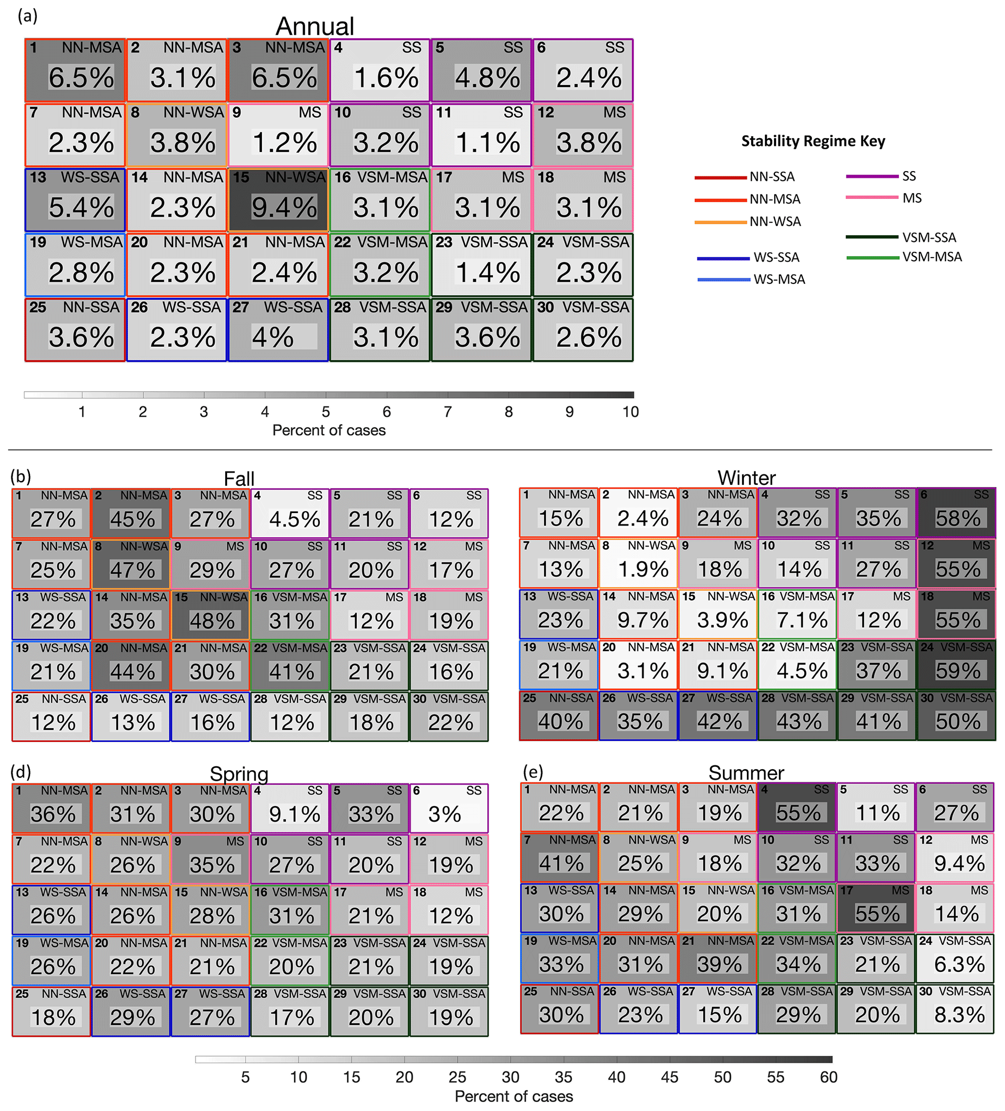
Figure 3 Grid plots following the same layout as the SOM indicating (a) the annual frequency of radiosonde profiles mapping to each pattern, as well as of all the cases mapped to a given pattern, the percent which occurred during (b) fall, (c) winter, (d) spring, and (e) summer, with shading corresponding to the greyscale color bars. The bold number in the upper left-hand corner of each subplot is the number of that pattern (1 through 30), and the letters in the upper right-hand corner of each subplot indicate that pattern's stability regime. Stability regime is also indicated by the color of the border for each subplot, following the colors given in the “stability regime key”.

The seasonal breakdown of SOM pattern frequency is displayed in Fig. 3b–e (e.g., 27 % of all radiosondes that map to pattern 1 occurred in the fall). Observations in the fall most heavily contribute to the SOM patterns in the center and left of the grid (patterns 2, 8, 15, 20, and 22). These are largely patterns with a well-mixed near-surface layer and moderate to strong stability aloft. Observations in the winter most heavily contribute to the SOM patterns in the far right and the bottom of the grid (patterns 5, 6, 12, 18, and 23 to 30). These are largely patterns with a near-surface θ_v inversion or a shallow well-mixed layer capped by a strong θ_v inversion.

Observations in the spring are more evenly distributed among all SOM patterns than any other season, as no SOM pattern contains more than 36 % of the total observations. The least common SOM patterns for spring are in the upper right of the grid (patterns 4, 6, and 18), which all have a near-surface θ_v inversion. Lastly, observations in summer most heavily contribute to two SOM patterns in the upper right of the grid (patterns 4 and 17), which are SS and MS respectively. Pattern 4 is particularly interesting, as there is strong near-surface stability and an elevated region of enhanced stability around 600 m a.g.l., which may be explained by unique processes occurring primarily in summer. Reported visibility and ceilometer observations suggest a possible low fog layer, formed from low-level warm air advection, and additional elevated cloud layer. Two patterns on the left side of the SOM (7 and 21, both NN-MSA) are also common in summer.

3.2 Wind speed characteristics for the SOM patterns

To understand the potential relationship between mechanical mixing and the stability structures presented by the SOM, we visualize average wind speed profiles for each SOM pattern; additionally, we analyze the LLJ characteristics for each pattern as the average across all individual cases in each pattern (Fig. 4). It is to be noted that, as LLJ core height and speed varies across the cases in each pattern, the LLJ is often smoothed out in the average wind speed profile. The LLJ frequency for all SOM patterns is similar, showing that an LLJ was present for 67 %–84 % of all observations mapped to any given pattern, with a median LLJ frequency of 76 %. Interestingly, the average LLJ height was found to be similar across all SOM patterns (roughly 400 m a.g.l.). The higher ABL heights of the weaker stability patterns (WS and NN; on the left side of the SOM) place the LLJ closer to the ABL top than for the stronger stability patterns with lower ABL heights (SS, MS, and VSM; on the right side of the SOM). Additionally, the interquartile ranges (IQR) of ABL height and LLJ height overlap for all patterns on the left half of the SOM, and for many patterns, the IQR of LLJ height extends below the average ABL height. Conversely, on the right half of the SOM, the IQR of ABL height and LLJ height do not overlap for any pattern (though they are close for pattern 23).

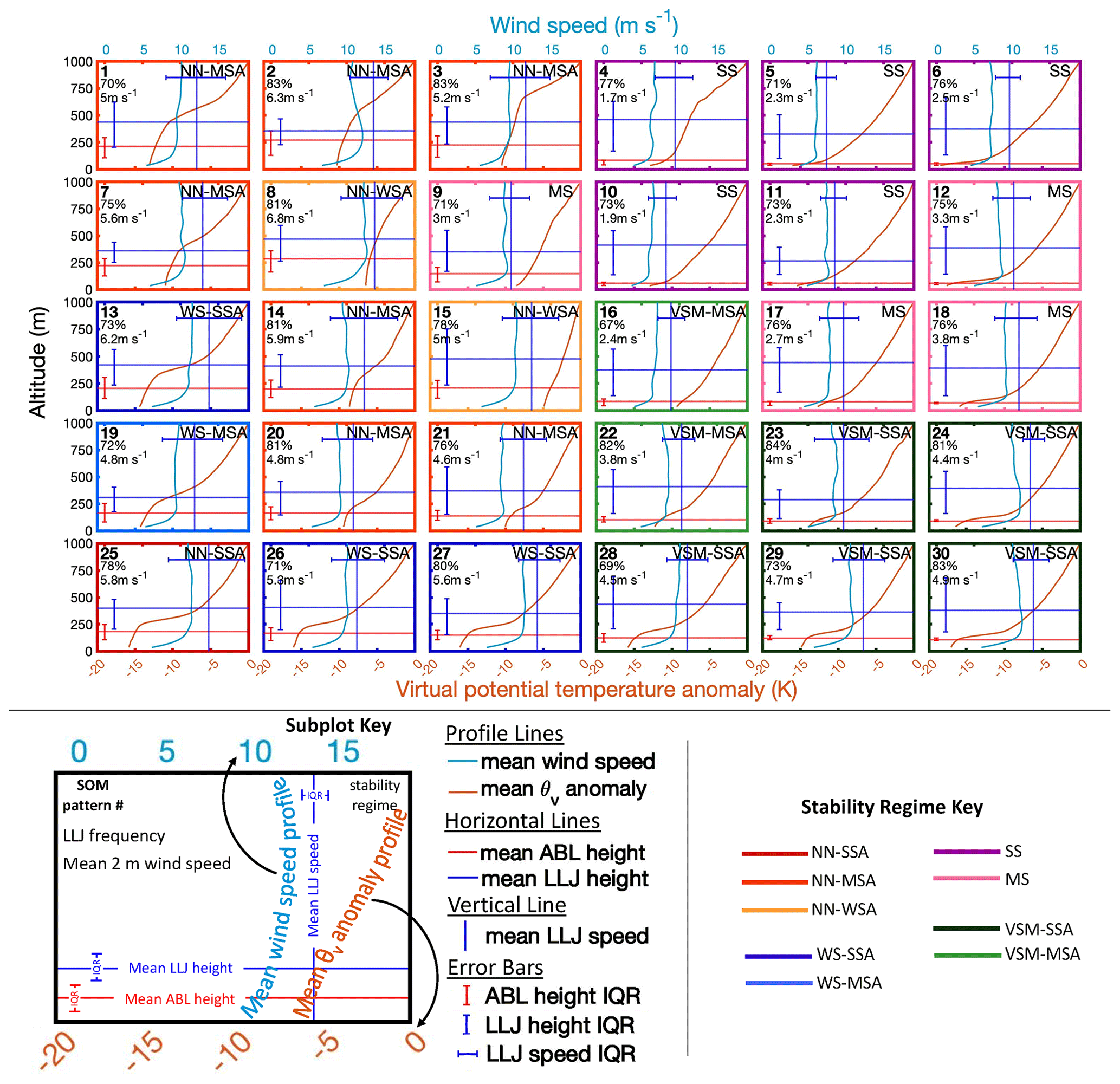
Figure 4 As in Fig. 2, but with mean virtual potential temperature (θ_v) anomaly profile (orange line, bottom x axis) and mean wind speed profile (baby blue line, top x axis) for all radiosonde profiles mapped to each SOM pattern. The horizontal red line in each subplot is the average ABL height, with the red error bar indicating the interquartile range (IQR). The horizontal blue line in each subplot is the average LLJ core height, with the vertically oriented error bar indicating the IQR. The vertical blue line in each subplot is the average LLJ core speed, with the horizontally oriented error bar indicating the IQR. Each subplot also has written the frequency of LLJs and average 2 m wind speed for that SOM pattern, written below the pattern number.

The LLJ core speeds, 2 m wind speeds, and overall wind speed profiles have greater values for the weaker stability regime patterns on the left half of the SOM (mean LLJ core speed of 12.3 m s⁻¹ and mean 2 m wind speed of 5.3 m s⁻¹), compared to the stronger stability regime patterns on the right half (mean LLJ core speed of 9.7 m s⁻¹ and mean 2 m wind speed of 3.3 m s⁻¹). For the patterns with a well-mixed layer above the surface (VSM, WS, and NN), the strength of the capping θ_v inversion is positively correlated to wind speed such that stronger stability aloft corresponds to greater LLJ core and 2 m wind speeds. For example, pattern 25 (NN-SSA) has average LLJ core speed and 2 m wind speed of 13.7 and 5.8 m s⁻¹ respectively, compared to pattern 20 (NN-MSA), which has average LLJ core speed and 2 m wind speed of 10.9 and 4.8 m s⁻¹ respectively. This relationship is also seen for the WS (stronger winds for patterns 13, 26, and 27 compared with 19) and VSM (stronger winds for patterns 23–24 and 28–30, compared with 16 and 22) patterns.

Analyzing the wind speed profiles that correspond to the vertical θ_v structure for each SOM pattern also helps to explain the subtle differences between SOM patterns. For example, at first glance, the θ_v anomaly profile for patterns 27 and 28 may look rather similar. However, per the stability regime criteria, pattern 27 is defined as WS, while pattern 28 is defined as VSM. On closer inspection, we see that LLJ frequency is greater and winds are stronger for pattern 27 (WS) than for pattern 28 (VSM), which explains the deeper ABL in pattern 27 (likely influenced by greater mechanical mixing). Across the SOM, LLJ core speed is lowest in the upper right-hand corner (SS and MS cases) and increases going down (VSM cases), to the right (WS cases), and up to the top left-hand corner (NN cases) of the SOM.

3.3 Moisture characteristics for the SOM patterns

Properties of clouds and moisture can impact vertical θ_v structure and stability due to their radiative effect and ability to decouple sub-cloud layers from the atmosphere above (e.g., clouds which form from long-range moisture transport are often separated from the ABL by a stable layer such that turbulence is not continuous between the ABL and the cloud). Thus, to understand the relationships between clouds and atmospheric moisture content and the stability structures presented by the SOM, we visualize average mixing ratio profiles for each SOM pattern; additionally, we analyze the cloud frequency (percent of individual cases in a given SOM pattern which had clouds), as well as the median CBH and LWP for each pattern (Fig. 5). We use the median rather than the mean for these characteristics, as the ranges in these values are quite large such that the mean can be heavily impacted by larger values and outliers, and thus the median is a more representative value. For most SOM patterns, the θ_v inversion corresponds with a moisture inversion (increase in mixing ratio with altitude) at about the same height, with the strength of the moisture inversion proportional to the strength of the θ_v inversion in most cases. There are however some exceptions where the moisture inversion is weak despite a moderate to strong surface-based θ_v inversion (e.g., patterns 5, 9, and 10). For the well-mixed layers (i.e., VSM, WS, and NN), below the elevated θ_v inversion, the mixing ratio is relatively constant with altitude or slightly decreasing. For pattern 15 (NN-WSA stability), there is no moisture inversion.

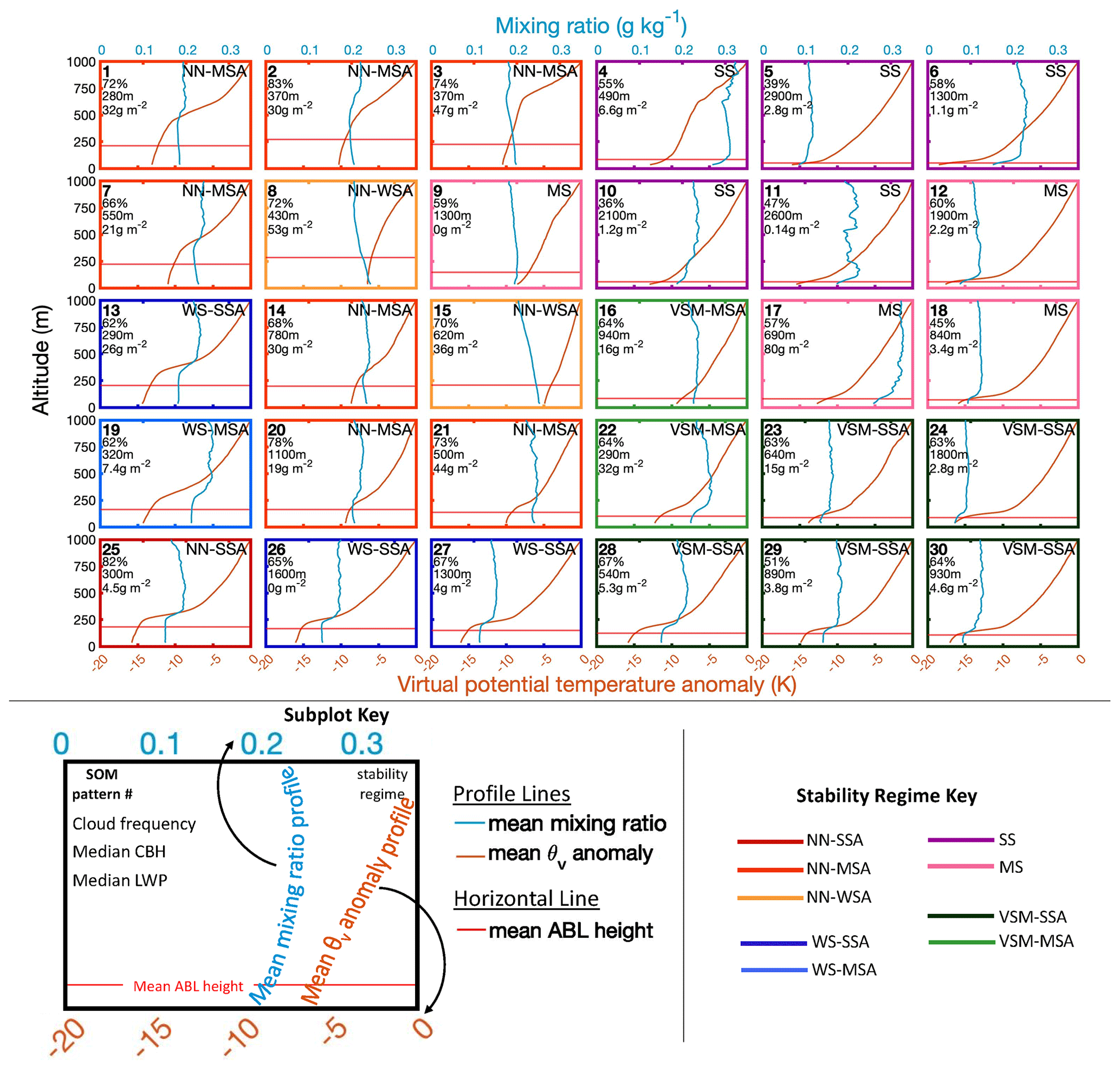
Figure 5 As in Fig. 2, but with mean virtual potential temperature (θ_v) anomaly profile (orange line, bottom x axis) and mean mixing ratio profile (baby blue line, top x axis) for all radiosonde profiles mapped to each SOM pattern. The horizontal red line in each subplot is the average ABL height. Each subplot also has written the frequency of clouds, median cloud base height (CBH), and median liquid water path (LWP) for that SOM pattern, written below the pattern number.

Cloud frequency varies across SOM patterns, though all patterns can occur in the presence of clouds, with a median overall cloud frequency of 64 %. The majority (78 % of clouds observed) were low clouds (i.e., CBH ≤2 km), with the highest seasonal frequency of clouds during fall (78 %) and the lowest seasonal frequency of clouds during spring (52 %). There was greater frequency for the SOM patterns with weaker stability either near the surface or aloft, the greatest being that for patterns 2 (NN-MSA stability with cloud frequency of 83 %) and 25 (NN-SSA stability with cloud frequency of 82 %). Pattern 10 (SS stability) had the lowest cloud frequency at 36 %. Perhaps the more important control on the θ_v structure is the height of the clouds and their liquid water content. CBH was highest for the patterns with stability of SS, with the exception of patten 4 (which likely formed due to low-level warm air advection, as discussed previously), followed by patterns with stability of MS. These patterns also have relatively low LWP. One exception is pattern 17, which was a common pattern in summer, with an LWP of 80 g kg⁻¹ and high mixing ratio throughout the profile, suggestive of larger-scale warm, moist air advection. For the patterns with a well-mixed layer above the surface (VSM, WS, and NN), lower CBH corresponds to a deeper well-mixed layer (e.g., pattern 13 versus pattern 26). Additionally, higher LWP values correspond with weaker stability both near the surface and aloft and a deeper well-mixed layer (e.g., pattern 1 versus pattern 25).

There is little relationship between ABL height, CBH, and the height of the moisture inversion. For patterns with surface-based θ_v and moisture inversions (SS and MS), CBH is typically over 2 km above the top of the ABL, but a correlation between the variables is not found. For patterns with elevated θ_v and moisture inversions (VSM, WS, and NN), in some cases the CBH is just above the ABL at a similar level with the elevated inversions. In other cases, the CBH is well above the ABL, which could be at, above, or below the level of the elevated inversions. This points to the varying cloud coupling or decoupling states with respect to the surface. For example, cases in the lower right of the SOM (VSM stability), in which CBH is well above the ABL, are more likely to reflect the cloud-surface decoupling state, whereas cases in the upper left of the SOM (NN-stability), in which CBH is just above the ABL, are more likely to reflect the cloud-surface coupling state.

3.4 Summary of ABL characteristics

The analysis in this final section transitions from the SOM-based perspective in the previous sections to a more simplistic grouping of radiosonde observations by stability regimes (as defined by Table 2) in order to more accurately determine stability regime frequency distribution and corresponding ABL characteristics. For Fig. 6, the regimes are organized from strongest to weakest near-surface stability going from left to right (where VSM is considered more stable than WS due to a shallower ABL), and within a given near-surface regime, the aloft regimes are also organized such that stability decreases from left to right.

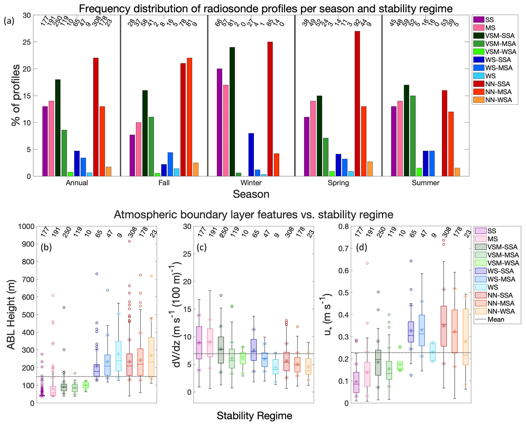
Figure 6 Top: (a) frequency distribution showing the percent of radiosonde profiles in each stability regime, annually and seasonally. For the seasonal sections, the percent shown is with respect to the total number of radiosonde profiles in that season. The numbers along the top of the plot, above each bar, indicate the total number of radiosonde profiles of that stability regime and season. Bottom: box and whisker plots showing the annual range of (b) ABL height, (c) $\mathrm{d}V/\mathrm{d}z$ over the depth of the ABL, and (d) u_∗ for each stability regime. The center line of each box is the median, and the outer edges of the boxes are the upper and lower quartiles. The whiskers show the range of values within 1.5 times the interquartile range from the top or bottom of the box, and outliers are shown with hollow circles. Asterisks are included at the mean, 10th percentile, and 90th percentile. Horizontal dotted black lines show the annual mean values of each variable. The number of cases in each stability regime are given along the top of the figure.

The annual and seasonal frequency of each stability regime is shown in Fig. 6a. The most frequent near-surface regime observed was NN (37 % of profiles), followed by VSM (27 % of profiles), MS (14 % of profiles), and SS (13 % of profiles). WS was observed less frequently (9 % of profiles). The total frequency of a stable ABL (combining SS, MS, and WS frequencies) was 36 %, just slightly less than the frequency of a near-neutral ABL. The most frequent regime observed aloft was -SSA (66 % of VSM cases, 54 % of WS cases, and 60 % of NN cases had strong stability aloft) followed by -MSA (31 % of VSM cases, 39 % of WS cases, and 35 % of NN cases had moderate stability aloft). Weak stability aloft was infrequently observed (3 % of VSM cases, 7 % of WS cases, and 5 % of NN cases had weak stability aloft). The overall most common regime was NN-SSA, followed by VSM-SSA.

In fall, the strongest stability regimes (SS and MS) were less frequent, while NN was more frequent than the annual frequency. Of all seasons, the winter stability regime frequency distribution is most different from the annual results. Winter had a higher frequency of the strongest stability regimes (SS, MS, and VSM-SSA), and the NN regime was more heavily dominated by NN-SSA. In spring, the relative frequencies of stability regime are very similar to those seen annually, the only major difference being a higher frequency of NN-SSA. Lastly, in summer, the relative frequencies of SS, MS, and VSM and NN with strong and moderate stability aloft were similar to one another.

Next, we present ABL height, change in horizontal wind speed between the surface and top of the ABL ($\mathrm{d}V/\mathrm{d}z$), and u_∗. The annual range of values of each of these variables for each stability regime is shown in Fig. 6b–d. Supplement Fig. S2 indicates when there is a statistically significant difference at the 5 % significance level between the mean values of each variable between all pairs of stability regimes. The determination uses a two-tailed t test when degrees of freedom (abbreviated as “df”) ≤100 and a two-tailed z test when df >100.

ABL height increases as stability decreases (Fig. 6b). A marked increase in ABL height separates the shallower SS, MS, and the VSM regimes (ABL height largely less than the mean) from the deeper WS and NN regimes (ABL height largely greater than the mean). The jump in ABL height between the VSM and WS regimes is in part a product of how we define the VSM regime (which requires an ABL height of 125 m or less). However, the magnitude of the increase in ABL height between the VSM (mean of 85 m) and WS regimes (mean of 221 m) demonstrates that this threshold was meaningful. Additionally, we find that ABL height increases as stability aloft decreases (e.g., the mean ABL height for WS-MSA is greater than the mean ABL height for WS-SSA).

SS and MS had the greatest (largely above average) wind shear ($\mathrm{d}V/\mathrm{d}z$) within the ABL (Fig. 6c). For the weaker stability regimes (WS and NN), winds vary less with height due to greater mixing, which is a common behavior of winds within a weakly stable or near-neutral ABL (Wallace and Hobbs, 2006). Figure 6d shows that u_∗ and thus turbulence increase with decreasing stability. Within the VSM, WS, and NN regimes, $\mathrm{d}V/\mathrm{d}z$ and u_∗ decrease with weakened stability aloft. Significant differences in $\mathrm{d}V/\mathrm{d}z$ and u_∗ between most pairs of stability regimes (Fig. S2b) highlight that turbulence properties are distinct for each regime. While perhaps an intuitive statement, it is important to confirm that physically meaningful differences in stability regimes classified largely based on thermal gradient are found for mechanical processes, as well as for turbulence measured by the met tower (a separate platform than the radiosondes used to classify stability regime). This confirmation supports the validity of the stability regime criteria defined in Sect. 2.4.

4 Discussion and conclusions

The work presented in this paper provides an overview of the vertical structure of the ABL and statistics about key thermodynamic and kinematic features of the central Arctic lower atmosphere in the context of vertical structure and stability regime, using data from the MOSAiC expedition. The SOM patterns (Fig. 2), frequency distribution of stability (Fig. 6a), and ABL height variability (Fig. 6b) highlight that near-surface stability during MOSAiC spanned from strongly stable with a shallow ABL to near neutral with a deep ABL, with stable and near-neutral conditions occurring with similar frequencies. Stability aloft ranged from strongly to weakly stable. These findings are consistent with Persson et al. (2002), Tjernström and Graversen (2009), and Brooks et al. (2017). The SOM reveals that within each stability regime category defined in the current paper (Table 2) the height and strength of the θ_v inversion can still vary greatly, and as such, the SOM reveals more nuances about the range of lower-atmospheric vertical structure than might be evident by a more simple stability regime classification. The variability of θ_v inversion height and strength for cases in the WS-MSA and NN-SSA regimes is however less than within the other regimes, as WS-MSA and NN-SSA are each represented by only one SOM pattern, whereas the other regimes are represented by multiple SOM patterns.

The most frequent stability regimes were those with strong or moderate stability either near the surface (SS and MS) or aloft (VSM-SSA, VSM-MSA, NN-SSA, and NN-MSA). Thus, we conclude that the central Arctic atmosphere over sea ice is inclined to include a strongly or moderately stable layer somewhere below 1 km a.g.l. and usually below 400 m (this contrasts with the mid-latitudes and tropical regions where the capping inversion is often as high as 1 to 2 km). Sometimes this strongly to moderately stable layer is within the ABL and sometimes it caps a well-mixed ABL, with the latter scenario occurring with higher frequency than the former, consistent with Tjernström and Graversen (2009). In the latter scenario, the depth of the well-mixed layer is highly variable, ranging from 38 m (minimum ABL height of a VSM case) to 914 m (maximum ABL height of an NN case). Weak stability either near the surface or aloft is the rarest condition (demonstrated by few WS or -WSA SOM patterns and low frequencies of the WS and -WSA regimes). Thus, a near-surface regime of WS may represent a transition state between the stronger (SS, MS, and VSM) and weaker (NN) stability regimes, and there are rarely conditions to support weak stability aloft (-WSA). Discovering both the most common and the least common stability regimes is equally as important for our overall understanding of the Arctic lower atmosphere.

Seasonal differences in SOM pattern (Fig. 3) and stability regime frequency distribution (Fig. 6a) highlight the varying environment in the central Arctic throughout the annual cycle. In fall, thinner sea ice results in more upward heat transfer from the ocean to the atmosphere and a higher frequency of low-level liquid-bearing clouds (Intrieri et al., 2002b). This weakens ABL stability, explaining why a higher frequency of NN and lower frequency of SS and MS cases were observed in fall. In winter, the lack of solar radiation and long periods of clear skies allow for persistent longwave cooling of the surface, explaining the higher frequency of SS, MS, and VSM cases observed then. In summer, warm moist air advection can contribute to either a stable or well-mixed ABL depending on location and timing within the advection event, which may explain why summer had similar frequencies of stronger stability (SS, MS, and VSM) and weaker stability (NN) cases. In spring, conditions characteristic of either winter or summer may occur, which is consistent with the spring stability regime distribution being most similar to the annual distribution and no SOM patterns being particularly dominant in spring.

The differing height, strength, and depth of the θ_v inversion across the SOM patterns can be explained by the corresponding wind and moisture features. In the following discussion, we first summarize the relationships between wind speed features and atmospheric stability. Average wind speed and LLJ characteristics for each SOM pattern (Fig. 4) and wind shear and u_∗ within the ABL (Fig. 6c–d) suggest important relationships between mechanical mixing and atmospheric stability and vertical structure. Wind shear and u_∗ within the ABL quantify mechanical turbulence near the surface, while the presence of an LLJ can enhance mechanical generation of turbulence aloft. Weaker winds (even in the case of an LLJ) and lower u_∗ values correspond to stronger near-surface stability, while stronger overall winds (and thus greater LLJ core speeds) and greater u_∗ values correspond to a weakly stable or near-neutral ABL. The magnitudes of these kinematic features are notably distinct between SS, MS, and the VSM regimes (right half of the SOM) and the WS and NN regimes (left half of the SOM), highlighting the importance of mechanically generated turbulence at differentiating the two groupings. This agrees with previous findings that stronger winds work to weaken stability in the ABL through the mechanical generation of turbulence (Banta, 2008). Despite weaker winds and lesser u_∗ for stronger near-surface stability, wind shear ($\mathrm{d}V/\mathrm{d}z$) over the depth of the ABL increases with increasing stability, revealing that in strong stability cases, static stability suppresses mechanically generated turbulence, promoting continued ABL stability despite high amounts of wind shear.

While LLJ core speed, 2 m wind speed, and u_∗ increase with decreasing near-surface stability, the opposite relationship is seen for stability aloft: LLJ core speed, 2 m wind speed, and u_∗ values are greatest when stability aloft is greatest. One possible explanation is that when the atmosphere is initially strongly stable (e.g., in the absence of clouds during winter), more wind shear is required to produce enough mechanically generated turbulence to fully mix out the near-surface layer than if the atmosphere is initially weakly stable (e.g., in the presence of clouds). Then the stable layer becomes elevated, separated from the surface by the mixed layer. Lastly, as the LLJ core is situated closer to the ABL for weaker stability regimes, this suggests greater coupling between the LLJ and the ABL for these cases, such that the wind shear associated with the LLJ contributes to the weakening of the ABL stability. Conversely, as the LLJ core is situated higher above the ABL for stronger stability regimes, the ABL and LLJ are more likely to be decoupled, and the strong static stability of these cases suppresses the mechanical turbulence generated by the wind shear.

The frequency of LLJs found in the current study is consistent with results of Tian et al. (2020) and ReVelle and Nilsson (2008) but exceeds that found in Jakobson et al. (2013), Lopez-Garcia et al. (2022), and Tuononen et al. (2015). The reasoning for the discrepancy between each of these studies varies. The difference in frequency from Jakobson et al. (2013) is likely due to the difference in sampling period between the two studies. The difference in frequency from Lopez-Garcia et al. (2022) is likely because LLJs with greater speeds may not have a jet core speed that is at least 25 % greater than the wind speed minimum above the LLJ core, and such cases were not considered in Lopez-Garcia et al. (2022). However, such LLJs can still be important because even if the winds are strong throughout the entire profile up to 1.5 km (for example, during a storm), the slightly greater core speed of the LLJ beyond that of the ubiquitously high winds throughout the column supports the production of increased turbulence in the ABL compared to without an LLJ. Lastly, the difference in frequency from Tuononen et al. (2015) is likely because the much lower vertical resolution of the Arctic System Reanalysis (ASR-Interim) data used in Tuononen et al. (2015) would miss shallow LLJ cases.

Mixing ratio profiles, cloud frequency, and median CBH and LWP for each SOM pattern (Fig. 5) highlight the occurrence of clouds in the central Arctic, as well as the relationships between CBH, atmospheric moisture, and stability. The SOM showed that there is typically a moisture inversion at the same altitude as the θ_v inversion, with moisture inversion strength proportional to θ_v inversion strength, which agrees with previous studies (Naakka et al., 2018; Devasthale et al., 2011; Nygård et al., 2014). The annual occurrence of clouds during MOSAiC was less than the annual average occurrence presented in Intrieri et al. (2002b). However, results of the current study agree with previous findings that clouds observed in the Arctic are typically low-level clouds. Low clouds, correlated with greater LWP, were observed with greater frequency for cases with weaker stability both within the ABL and aloft. This highlights the ability of low clouds and enhanced liquid water content to support the weakening of stability near the surface by warming the near-surface atmosphere, as well as weakening stability aloft due to turbulent mixing below cloud base through cloud top radiative cooling.

The varying depth of a well-mixed layer is likely a function of whether the ABL is coupled to a stratocumulus cloud layer: a coupled cloud supports a deeper ABL that is well-mixed up to cloud base (with the mixed layer extending to cloud top), whereas a decoupled cloud is separated from a shallower ABL by a θ_v inversion below cloud base (Brooks et al., 2017). Therefore, comparing ABL height to CBH suggests whether the surface and the cloud may be coupled or decoupled. The patterns in the lower right of the SOM with VSM stability have a shallower ABL capped by a θ_v inversion, with CBH several hundred meters above the ABL, suggesting surface–cloud decoupling. The patterns in the upper left of the SOM with NN stability have a deeper ABL with CBH often below the altitude of the θ_v inversion, suggesting surface–cloud coupling. For these patterns, which also have stronger winds, we theorize that the combination of relative warming of the near-surface atmosphere from the clouds and the mechanical turbulence generated from wind shear allows for vertical mixing of the near-surface layer, which is strong enough to reach the level at which downward-propagating buoyant turbulence from cloud top cooling is present, creating a well-mixed layer between the surface through the cloud. Conversely, for stronger stability cases with a high CBH, the cloud and surface are completely decoupled such that the cloud is unlikely to impact the surface, and the strong stability persists. This discussion agrees with Sotiropoulou et al. (2014), who found that decoupled clouds typically occur at higher altitudes. However, the aforementioned discussion is at this point only educated speculation, and additional analysis based on the equivalent potential temperature profiles is required to confirm the cloud coupling or decoupling state.

One limitation of this study is that stability regimes are based on radiosonde profiles starting at 35 m, since measurements below this are often unreliable, so differences in stability below this height are neglected (and potentially important). A complementary paper (Jozef et al., 2023b) delves deeper into the impact of atmospheric radiative and mechanical forcings on ABL stability and how these relationships vary by season, with a focus on the peculiarities of summer processes through additional analysis of the synoptic setting, surface radiation budget, near-surface mixing ratio, and fog observations. Therefore, such results are not addressed in this work. Future work will be conducted to determine how well the observed results are represented by weather and climate models. Thus, we hope that these findings serve to help inform the improvement of parameterizations of the central Arctic in weather and climate models.