CO₂ and CO temporal variability over Mexico City from ground-based total column and surface measurements

Accurate estimates of greenhouse gas emissions and sinks are critical for understanding the carbon cycle and identifying key drivers of anthropogenic climate change. In this study, we investigate the variability in CO and CO₂ concentrations and their ratio over the Mexico City metropolitan area (MCMA) using long-term, time-resolved columnar measurements at three stations, employing solar-absorption Fourier transform infrared spectroscopy (FTIR). Using a simple model and the mixed-layer height derived from a ceilometer, we determined the CO and CO₂ concentrations in the mixed layer from the total column measurements and found good agreement with surface cavity ring-down spectroscopy measurements. In addition, we used the diurnal pattern of CO columnar measurements at specific time intervals to estimate an average growth rate that, when combined with the space-based Tropospheric Monitoring Instrument (TROPOMI) CO measurements, allowed for the derivation of annual CO and CO₂ MCMA emissions from 2016 to 2021. A CO emission decrease of more than 50 % was found during the COVID-19 lockdown period with respect to the year 2018. These results demonstrate the feasibility of using long-term EM27/SUN column measurements to monitor the annual variability in the anthropogenic CO₂ and CO emissions in Mexico City without recourse to complex transport models. This simple methodology could be adapted to other urban areas if the orography of the regions favours low ventilation for several hours per day and the column growth rate is dominated by the emission flux.

1 Introduction

The greenhouse gas (GHG) mitigation strategies implemented in megacities following the 1997 Kyoto Protocol and the 2015 Paris Agreement play a crucial role in the global action plan to mitigate climate change, given that cities are accountable for more than 70 % of global anthropogenic emissions (Duren and Miller, 2012). With the recent progress in space-based and ground-based remote GHG measurements in terms of accuracy, spatial coverage, resolution and temporal frequency, GHG emissions can increasingly be constrained by comparing bottom-up and top-down estimates. Top-down approaches are generally based on ground- or space-based atmospheric measurements coupled with inverse modelling, using 3D Eulerian (i.e. WRF-Chem) or Lagrangian and hybrid (i.e. X-STILT and HYSPLIT) approaches (Wu et al., 2018; Che et al., 2022; Lian et al., 2023). The quantification of anthropogenic CO₂ enhancements from cities using satellite data, e.g. GOSAT (Wang et al., 2019), OCO-2 (Ye et al., 2020) or TanSat (Liu et al., 2018), is still challenging due to the sparsity of the observations, the low signal from the anthropogenic contribution compared with the background levels and biogenic contribution, and some inconveniences inherent to space-based measurements, such as the non-negligible aerosol effects (Wang et al., 2020, and references therein). Some studies have estimated the urban enhancements of anthropogenic CO₂ concentrations along with CO and NO₂ from satellite measurements, as these air pollutants can serve as tracers of anthropogenic CO₂ (Silva et al.,2013; Park et al., 2021, and references therein). The $\mathrm{CO}/{\mathrm{CO}}_{\mathrm{2}}$ ratio is often used to determine the combustion efficiency of the cities (Park et al., 2021, and references therein). With the development of a new generation of space-based observatories, such as Sentinel-5P and OCO-2/OCO-3, the evolution of GHGs at the city scale can now be characterized at a finer temporal and spatial resolution (Kiel et al., 2021), although more validation efforts are needed. As inverse modelling is likely undermined by the approximations used to define the emission patterns, transport processes and meteorology, top-down approaches may lead to discrepancies in emissions estimates, in particular at sites with complex orography.

Ground-based total column Fourier transform infrared spectroscopy (FTIR) instruments provide valuable long-term concentration measurements of GHGs, reactive pollutant species and anthropogenic tracers, constituting a key element to validate regional and local inventories. Some studies have reported estimates of CO₂ and CH₄ emissions from large urban areas (Babenhauserheide et al., 2020, in Tokyo; Hedelius et al., 2018, in the Californian South Coast Air Basin), using data from high-resolution FTIR instruments (i.e. Bruker IFS120/5HR) contributing to the Total Column Carbon Observing Network (TCCON). Nevertheless, only a few TCCON stations are located in urban areas (Toon et al., 2009; Chevallier et al., 2011; Sussmann and Rettinger, 2020). The development of the COllaborative Carbon Column Observing Network (COCCON; Frey et al., 2019), using a new generation of portable low-spectral-resolution FTIR (EM27/SUN) spectrometers (Gisi et al., 2012; Hase et al., 2016) that are able to simultaneously measure the CO₂, CO, H₂O and CH₄ average total columns with a similar quality to that of TCCON, has considerably densified the number of measurements in urban environments. Some studies have reported emission estimates for big cities by means of the deployment of several EM27/SUN instruments at strategic sites throughout the cities (Hase et al., 2015, and Zhao et al., 2019, in Berlin; Vogel et al., 2019, in Paris; Makarova et al., 2021, in Saint Petersburg; Zhou et al., 2022, in Beijing and Xianghe; Che et al., 2022, in Beijing; Rißmann et al., 2022, in Munich), coupling columnar measurements with inverse modelling. Most of these studies have been based on short-term campaign observations, applying the differential column methodology (DCM; Chen et al., 2016) or dedicated dispersion models (Hase et al., 2016), coupled with simple mass-balance-based methods or inverse modelling to derive emissions. Most of these studies have reported significant discrepancies between the estimates, depending on the models used (Viatte et al., 2017).

In this study, we aimed to determine CO₂ and CO emissions in the Mexico City metropolitan area (MCMA) using ground-based FTIR and surface measurements, without resorting to complex dispersion and/or chemistry transport models. The MCMA, with a population of around 22 million inhabitants, is in the top 10 most populous cities in the world and ranks among the major emitters of GHGs in North America. The available information on GHG emission estimates is mainly based on the inventories reported by the Ministry of the Environment of Mexico City (SEDEMA); this information is updated every 2 years but lags several years behind. In the report based on 2018, the latest published before the COVID-19 lockdown (2020), a total emission of 75.2 Mt CO₂-eq (carbon dioxide equivalent) is estimated for the MCMA, 87 % of which is attributed to fossil fuel combustion and 58 % of which originates from the transport sector (Secretaría del Medio Ambiente de la Ciudad de México, 2018). The Mexico City government is actively engaged in the C40 climate change programme and has implemented significant policy measures since 2008, including promoting sustainable transportation systems, implementing energy efficiency measures, increasing the use of renewable energy sources and adopting green building practices. On a national scale, the country is committed to reducing its GHG emissions by 35 % by 2030 with respect to its base level, as stated in the last nationally determined contributions report (NDC 2022, UNFCCC, https://unfccc.int/ndc-synthesis-report-2022, last access: 21 October 2024). To assess the effect of the national and local mitigation policies, the installation of ground-based GHG measurement networks and the refinement of bottom-up estimates by comparing them with the top-down method (i.e. inverse modelling) is of critical importance to obtain a comprehensive GHG database that can serve as a follow-up with respect to mitigation actions.

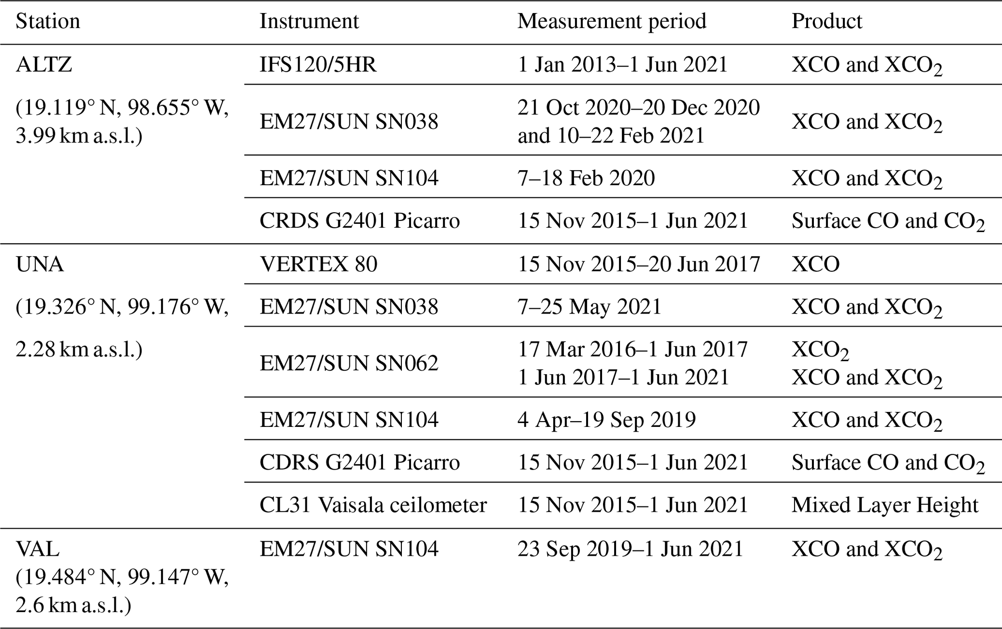
Table 1 Instrumentation and measurement periods used in this study.

Within the framework of research projects related to air quality assessment, atmospheric monitoring and satellite product validation, the Institute of Atmospheric Sciences and Climate Change (ICAyCC, Spanish acronym) at UNAM (Universidad Nacional Autónoma de México) has deployed a wide range of surface gas sensors and ground-based remote-sensing instruments across the MCMA over the last decade (Grutter et al., 2003; Molina et al., 2010; Bezanilla et al., 2014; Stremme et al., 2009; 2013; Baylon et al., 2017). Since 2013, UNAM has contributed to the Network for the Detection of Atmospheric Composition Change (NDACC), performing continuous composition measurements of the free troposphere from the high-altitude Altzomoni Atmospheric Observatory (ALTZ), located 60 km southeast of Mexico City at 3985 $\mathrm{m}\mathrm{a}.\mathrm{s}.\mathrm{l}.$ (metres above sea level). Baylon et al. (2017) reported the background CO₂ variability and trend from this station between 2013 and 2016. Stremme et al. (2013) reported the first top-down estimate of CO emissions for the MCMA, based on FTIR CO total column measurements and Infrared Atmospheric Sounding Interferometer (IASI) data. These authors derived the CO₂ emissions for the MCMA using the CO emission estimates and the average $\mathrm{CO}/{\mathrm{CO}}_{\mathrm{2}}$ ratio reported in Grutter (2003), employing FTIR measurements. In 2018, the Mexican–French “Mexico City's Regional Carbon Impacts (MERCI-CO2)” project (coordinated by UNAM and the Laboratoire des Sciences du Climat et de l'Environnement) was launched with the aim of assessing the CO₂ emissions from MCMA using EM27/SUN measurements and inverse modelling to evaluate the effectiveness of the mitigation strategies implemented by the local authorities. Xu (2023) examined the performance of a modelling system based on WRF-Chem to assess whole-city emissions using EM27/SUN measurements obtained within the framework of the MERCI-CO2 project. However, the complex orography of the region posed a challenge in the atmospheric transport simulations and, thus, for the top-down estimates using inverse modelling. Indeed, Mexico City is situated in a high-altitude basin (∼ 2300 $\mathrm{m}\mathrm{a}.\mathrm{s}.\mathrm{l}.$), surrounded by mountains reaching up to 5.6 $\mathrm{km}\mathrm{a}.\mathrm{s}.\mathrm{l}.$, and is prone to the accumulation of anthropogenic emissions, especially during the dry season, when the atmospheric boundary layer ventilation is limited (Burgos-Cuevas et al., 2023). The boundary layer dynamics in the basin and the wind surface circulation are complex, due to the temperature contrasts and rough topography.

In this study, we report the long-term (2013–2021) variability in the CO₂ and CO total columns and surface concentrations (from 2014) over the MCMA using ground-based FTIR and surface cavity ring-down spectrometer (CRDS) measurements. Using mixed-layer height data from the continuous ceilometer measurements at UNAM, we examined the consistency of the surface and total column measurements of our network. We also determined an average $\mathrm{CO}/{\mathrm{CO}}_{\mathrm{2}}$ ratio based on FTIR and surface measurements at different (from daily to intraday) temporal resolutions. Then, using the spatial distribution of Tropospheric Monitoring Instrument (TROPOMI) CO column measurements, we explored the potential of our FTIR network to capture the CO and CO₂ emission variability in the megacity using a simplified model, i.e. without recourse to complex numerical simulations. Our estimates are compared with the available bottom-up and previous top-down estimates.

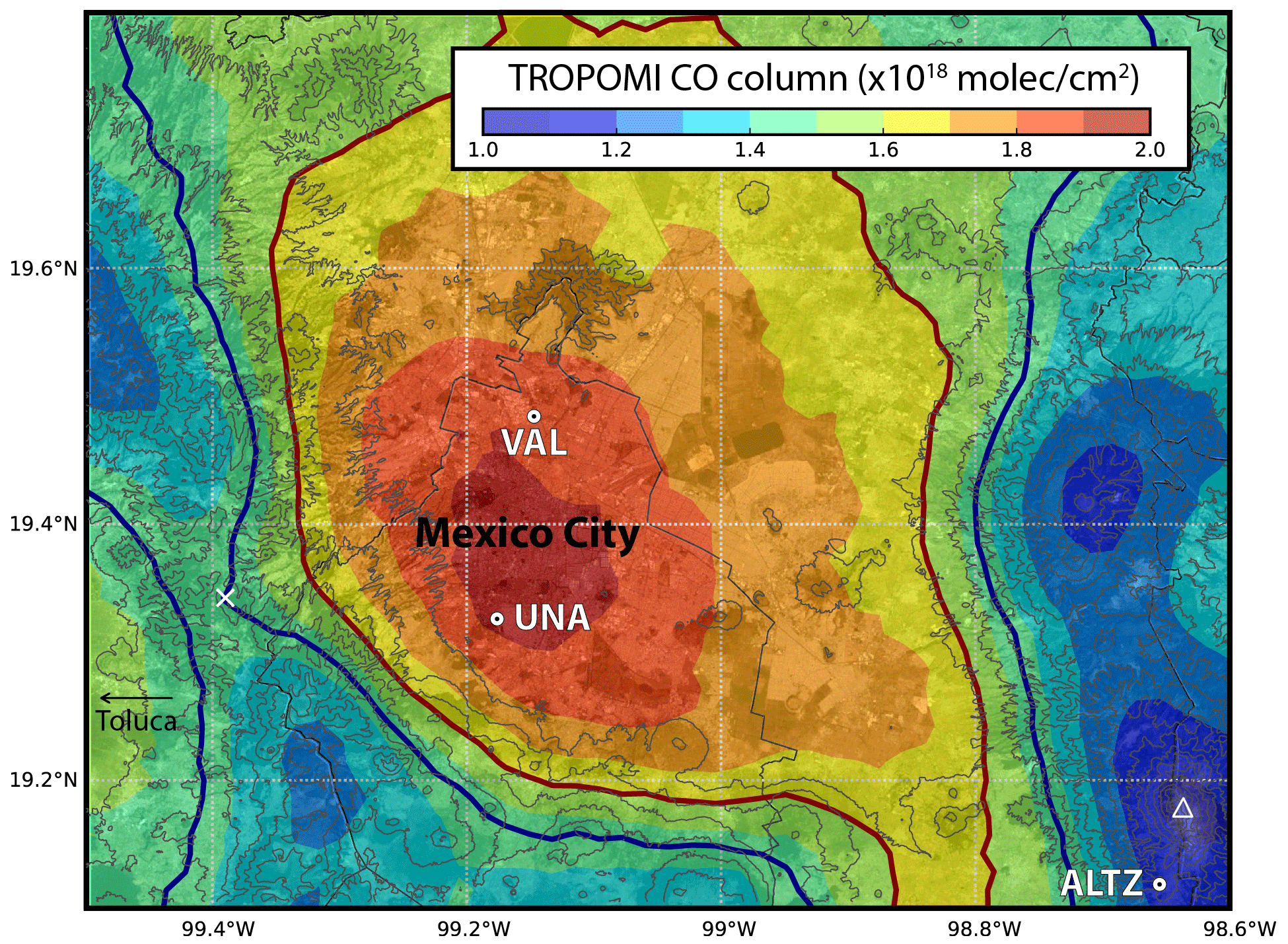
Figure 1 Map of the ALTZ, UNA and VAL stations as well as the average distribution (2018–2022) of carbon monoxide total columns over the Mexico City metropolitan area (MCMA) calculated from the TROPOMI CO product. Red and blue contour lines represent the respective inner and outer areas used to calculate the effective area (see details in the text). The cross symbol indicates the smallest CO total column value observed upwind of the city at the elevation of the Basin of Mexico, which is used to estimate the background. The average total column can be decomposed into two main contributors: (i) a background of around 1.45 × 10¹⁸ $\mathrm{molec}.{\mathrm{cm}}^{-\mathrm{2}}$ (limits represented by blue contour lines) and (ii) the local influence corresponding to the CO emitted on the same day. The total columns are highly influenced by the topography that is clearly visible over the highest terrain of the region, near the Popocatépetl and Iztaccíhuatl volcanoes to the southeast of Mexico City. The mountains of Ajusco are located southwest of Mexico City. The enhancement in the centre of the metropolitan area reflects the CO locally emitted on the same day.

2 Sites, instrumentation and measurement protocols

In this work, we used (1) the column-averaged dry-air mole fractions of CO₂ and CO (XCO₂ and XCO, respectively) from three permanent FTIR stations distributed within a radius of 100 km around MCMA (Fig. 1) and (2) the surface measurements performed at the UNA and ALTZ sites. The measurement periods for the different instruments at each site are reported in Table 1. The first permanent station, UNA, is situated to the south of the city on the main campus of UNAM. The second station, the ALTZ background site (3985 m a.s.l.), is located 60 km east-southeast of UNAM, within the Iztaccíhuatl–Popocatépetl National Park. The third station, VAL, is located in the northern part of the city in a highly industrialized zone. The equipment at the different stations and the measurement protocols are described in the following subsections.

2.1 UNA station: total column, surface concentration and mixed-layer height measurements

Atmospheric total columns of several gas species, such as O₃, NH₃, CH₄, CO and HCHO, have continuously been measured at UNA since 2010 (Bezanilla et al., 2014; Plaza-medina et al., 2017; Baylon et al., 2017; Rivera Cárdenas et al., 2021; Herrera et al., 2022) using solar-absorption FTIR spectroscopy.

Measurements are performed in the mid-infrared (MIR) and near-infrared (NIR) spectral ranges using a Bruker VERTEX 80 spectrometer. The instrument has a maximum optical path difference (MPD) of 12 cm (corresponding to a spectral resolution of 0.075 cm⁻¹) and is equipped with two detectors, a liquid-nitrogen-cooled mercury–cadmium–telluride (MCT) detector and an indium–gallium–arsenide (InGaAs) detector. Solar-absorption measurements are performed using a custom-built solar tracker. A full description of the instrumental set-up and measurement protocols is given in Bezanilla et al. (2014) and Plaza-Medina et al. (2017). The CO measurements are routinely performed in the MIR spectral range with a spectral resolution of 0.075 cm⁻¹, using the MCT detector.

In March 2016, an EM27/SUN spectrometer was implemented at UNA to continuously measure XCO₂, XCH₄, XH₂O and XCO total columns from solar NIR spectra with a spectral resolution of 0.5 cm⁻¹ (MPD of 1.8 cm). The spectrometer is equipped with its own solar tracker (Bruker CAMTracker; Gisi et al., 2011) that captures and redirects the solar beam into a RockSolid™ pendulum interferometer equipped with a Quartz beam splitter. The EM27/SUN installed at the UNA station (SN 62, hereafter EM27-SUN_62) was initially operated with a standard InGaAs-diode detector sensitive to the 5500–11000 cm⁻¹ spectral range, to which a second InGaAs detector with a Ge filter was added in 2017 for CO measurements through a second channel (4000–5500 cm⁻¹) (Hase et al., 2016). Further details on the technical characteristics and systematic performance evaluation of the EM27/SUN spectrometer are given in Frey et al. (2019) and Alberti et al. (2022). The spectrometer was installed in a custom-made protective box, including a remotely controlled dome cover, a GPS and a PCE-THB-40 data logger for precise timing and surface pressure measurements. Double-sided forward–backward interferograms (IFGs) are routinely recorded with a scanner velocity of 10 kHz; thus, the recording time of one measurement (averaging 10 IFG scans) is close to 1 min.

Additionally, CO₂, CO, CH₄ and H₂O surface measurements are continuously performed at the UNA station using a cavity ring-down spectrometer (CRDS; model G2401, Picarro Inc.). The CRDS uses a laser to quantify the spectral features of gas-phase molecules in an optical cavity, offering an absorption path length of up to 20 km. Frequency shifts are prevented with a high-precision wavelength monitor, and temperature and pressure are precisely controlled by the analyser. Quantification is improved by the simultaneous spectral analysis of the measured gases. A calibration system using three gas standards provided by the National Oceanic and Atmospheric Administration Earth System Research Laboratory (NOAA ESRL), traceable to the WMO2007 scale, was set up at UNA in 2018 and at ALTZ in 2019. Data collected before the installation of the calibration systems were corrected with calibration coefficients obtained in 2018. The sampling inlet using Synflex tubing was placed at 24 $\mathrm{m}\mathrm{a}.\mathrm{g}.\mathrm{l}.$ at UNA station and includes a Nafion air dryer, as described in detail by González del Castillo et al. (2022). Data are continuously collected at a 0.3 Hz rate, and their uncertainties, calculated as the standard deviation of raw data over 1 min intervals when measuring calibration gases, are equal to 0.03 ppm at UNA (González del Castillo et al., 2022).

Finally, continuous mixed-layer height (MLH) measurements have been performed at UNA since 2008 using a CL31 ceilometer instrument (Vaisala). This is a robust commercial instrument that emits light pulses at a 10 kHz repeating frequency at 910 nm using an InGaAs diode laser. It detects the backscattered signal through a single lens with a silicon avalanche photodiode. The resulting backscatter profiles have a vertical resolution of 10 m and reach an altitude of 7500 m. The profiles have been used to retrieve the MLH above the city since 2011 (García-Franco et al., 2018).

2.2 ALTZ background station: total column and surface measurements

In 2012, the Altzomoni Atmospheric Observatory (ALTZ) was equipped with a high-resolution FTIR spectrometer (model IFS120/5HR, Bruker) that is capable of measuring atmospheric spectra in the NIR and MIR spectral regions with a 257 cm MPD, equivalent to a spectral resolution of 0.0035 cm⁻¹. The instrument was installed into a container with a motorized dome cover on the roof and a microwave communication system (60 km line of sight to the university campus); this allows full remote control of the instruments. When the dome is open, a solar tracker (CAMTracker; Gisi et al., 2011; Gisi, 2012) collects the solar beam and orients it toward the spectrometer entrance. The spectrometer can be operated with KBr or CaF₂ beam splitters and three different detectors (MCT; indium–antimonide, InSb; and InGaAs), and a set of seven optical filters is installed on a rotating wheel. The measurement routine consists of the acquisition of high-resolution (0.005 cm⁻¹), medium-resolution (0.02 cm⁻¹ and 0.1 cm⁻¹) and low-resolution (0.5 cm⁻¹) spectra in the NIR and MIR spectral ranges using the different NDACC filters (∼ 40 min for a complete sequence).

The NIR CO and CO₂ spectra (0.02 cm⁻¹) used in this study were recorded as the average of two scans taken for approximately 38 s with a scanner speed of 40 kHz. The MIR CO spectra (0.005 cm⁻¹) are deduced from the co-addition of six scans (< 200 s) with a scanner speed of 40 kHz. Due to a spectrometer laser replacement, the IFS120/5HR measurements were interrupted between November 2020 and January 2021. To avoid an important gap in the measurements, an EM27/SUN (EM27/SUN_38) was temporarily installed at the station during this period (Table 1). The intercalibration factors used for combining the two types of measurements were determined from previous side-by-side measurements performed during February 2021 (see Sect. 3.1.3 in the following and Table S1 in the Supplement).

In 2014, a CRDS (model G2401, Picarro Inc.) instrument was implemented at ALTZ; since then, it has been providing continuous CO₂, CO, CH₄ and H₂O surface measurements (Gonzáles del Castillo et al., 2022). The sampling inlet, using Synflex tubing, was placed at 4 $\mathrm{m}\mathrm{a}.\mathrm{g}.\mathrm{l}.$ and includes a Nafion air dryer (similar installation to UNA). A calibration system similar to that implemented at UNA, using three NOAA ESRL gas standards, was set up in 2019. The station also includes meteorological instruments, pressure and temperature sensors, and visible cameras, among other instrumentation for atmospheric and environmental monitoring.

2.3 VAL station: total column measurements

VAL station, located in Vallejo in the northern part of the MCMA, is part of the city's air quality network (RAMA) run by SEDEMA. An EM27/SUN spectrometer (EM27/SUN_104) and surface CO₂ sensor were installed at this station in 2019. The VAL spectrometer has been performing measurements with the two detectors since November 2019. Additionally, the VAL site includes a low-cost, medium-precision CO₂ sensor, installed as a part of a network implemented during the MERCI-CO2 campaign. It consists of a nondispersive-infrared-type sensor (model HPP3, Senseair) that can measure in the 0 to 1000 ppm range; after a calibration and target gas follow-up procedure, this sensor can produce data with < 1 % accuracy (Porras et al., 2023).

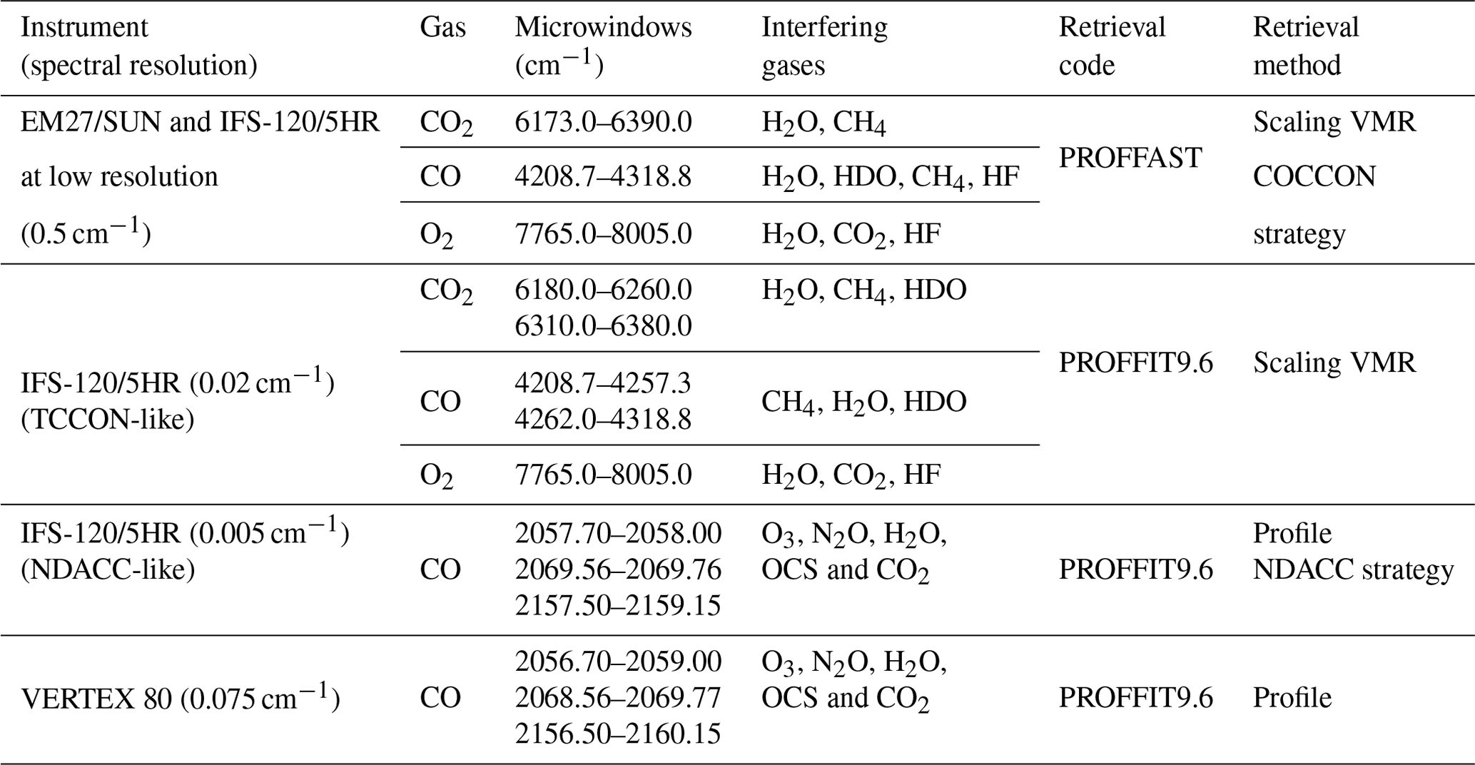
Table 2 FTIR analysis: description of the different FTIR products, retrieval strategies and parameters used in this study.

3 Data analysis

3.1 FTIR data processing and analysis

In this study, we used the solar-absorption measurements acquired by five different FTIR instruments (i.e. three EM27/SUN, a VERTEX 80 and an IFS120/5HR) to estimate the XCO₂ and the XCO total columns at each station. The retrieval strategies were adapted as a function of the spectral resolution and averaging kernel of each species. Table 2 summarizes the different products used in this study as well as their retrieval parameters.

3.1.1 EM27/SUN spectral analysis

Double-sided interferograms from the EM27/SUN were analysed using the PREPROCESS and PROFFAST codes following the standardized COCCON protocol; these codes have been developed by the Karlsruhe Institute of Technology (KIT) and are freely available (https://www.imk-asf.kit.edu/english/COCCON.php, last access: 14 October 2024). The codes and retrieval methods are fully described in Sha et al. (2020), Frey et al. (2021) and Alberti (2023); therefore, they are only briefly summarized here. The PREPROCESS algorithm generates the required spectra by a fast Fourier transform. The processing incorporates various quality checks, such as a signal threshold, intensity variations during recording and the requirement for proper spectral abscissa scaling, and it only generates spectra from raw measurements passing all of the checks (with the remaining ones being flagged). We used the instrumental line shape (ILS) parameters (i.e. modulation efficiency amplitude and phase error) reported on the KIT COCCON website (https://www.imk-asf.kit.edu/english/COCCON.php, last access: 14 October 2024) and in Alberti et al. (2022), corresponding to the initial KIT calibration of the spectrometers (Frey et al., 2019; Alberti et al., 2022). The PROFFAST-PCXS module (i.e. forward model of PROFFAST) pre-calculates daily lookup tables of the molecular absorption cross sections according to the meteorological parameters and trace gas volume mixing ratio (VMR) profiles' priors. The latest PROFFAST-PCXS version uses the HITRAN 2020 spectroscopic line lists (with some extensions, e.g. line mixing parameters added for CH₄). Here, we used the standard COCCON line lists as incorporated in the previous PROFFAST version, i.e. HITRAN 2008 for CH₄, HITRAN 2012 for CO₂, a modified version of HITRAN 2009 by Toon (2014, https://tccon-wiki.caltech.edu/Main/Spectroscopy, last access: 14 October 2024) for H₂O, a TCCON standard line list for O₂ and the same solar line list as previously used by TCCON (compiled by G. C. Toon, https://tccon-wiki.caltech.edu/Main/Spectroscopy, last access: 14 October 2024, for GGG2014). The least-squares fitting code PROFFAST-INVERS retrieves the total columns by scaling the prior VMR profiles iteratively until the fit is adjusted to the measured spectra. The intraday variability in the surface pressure is considered in the retrieval, interpolated from the in situ pressure measurements. To tie the column-averaged abundances provided by COCCON to TCCON data, PROFFAST applies post-process air-mass-dependent (ADCF) and air-mass-independent (AICF) corrections, independent of the instrument, similar to those used in the TCCON process (Sha et al., 2020, and Alberti, 2023). The corrections and parameters used are reported on the COCCON website and in Alberti (2023).

We automatized and adapted the data processing to obtain a preliminary “real-time” analysis that was updated hourly (hereafter referred to as AN1) for each site, in addition to the off-line treatment (hereafter referred to as AN2) applying the standard COCCON procedure. The meteorological data used in the AN1 retrieval were derived from the radiosonde data that were available daily, provided by Servicio Meteorológico Nacional (SMN) from measurements performed in the early morning (06:00 LT) at the Mexico City International Airport. The AN1 strategy adopted fixed VMR priors for each species, consisting of the averaged profile of a 41-year (1980–2020) run of the Whole Atmospheric Community Climate Model (WACCM), as commonly used in the NDACC community. The AN2 processing, generating the COCCON standard products, used the GGG2014 daily TCCON meteorological data and priors (referred to as map files), downloaded from the Caltech server, which are based on National Centers for Environmental Prediction (NCEP) reanalysis. For both AN1 and AN2 processing, we used the in situ intraday surface pressure measurements from the PCE-THB-40 sensors. A correction factor was applied to the pressure measurements to account for the bias between the different pressure sensors used, previously intercompared by a few days of side-by-side measurements.

CO₂, O₂, and CO were analysed in the 6173.0–6390.0, 7765.0–8005.0 and 4208.7–4318.8 cm⁻¹ spectral windows, respectively. The XCO₂ and XCO column-averaged dry-air mole fractions were calculated using the O₂ retrieved total columns, according to Wunch et al. (2009):

$$\begin{array}{}\text{(1)}& \mathrm{Xgas}=\mathrm{0.2095}(C_{\text{gas}}/C_{{\mathrm{O}}_{\mathrm{2}}}),\end{array}$$

where C_gas and $C_{{\mathrm{O}}_{\mathrm{2}}}$ are the target gas and O₂ total columns, respectively.

The real-time (AN1) and COCCON (AN2) XCO₂ and XCO products showed relative differences lower than 0.05 % and 5 %, respectively. The results presented hereafter are based on the official COCCON products (AN2 analysis).

3.1.2 VERTEX 80 and IFS120/5HR spectral analysis

High-resolution (0.005 cm⁻¹) and medium-resolution (0.02 and 0.075 cm⁻¹) solar-absorption spectra are processed using the PROFFIT9.6 code (Hase et al., 2004).

XCO₂ is retrieved from the NIR 0.02 cm⁻¹ resolution spectra by applying the procedure described in Baylon et al. (2017), in which two independent CO₂ and O₂ VMR scaling retrievals are performed using fixed WACCM VMR priors and NCEP-derived meteorological data. Spectral windows and interfering gases (Table 2) are similar to those used in the standard TCCON procedure. XCO₂ is then calculated from the retrieved CO₂ and O₂ total columns by applying Eq. (1).

For the ALTZ analysis, CO was retrieved from the high-resolution (0.005 cm⁻¹) spectra in the MIR region using the standard NDACC procedure (Pougatchev et al., 1998; Rinsland et al., 1998; Table 2). This procedure employs a profile retrieval strategy with fixed WACCM VMR priors and NCEP meteorological data. As the O₂ species is not analysed in the MIR region, the XCO was determined using the dry-air columns (C_dryair):

$$\begin{array}{}\text{(2)}& \mathrm{XCO}={\displaystyle \frac{C_{\mathrm{CO}}}{C_{\text{dryair}}}},\end{array}$$

where

$$\begin{array}{}\text{(3)}& C_{\text{dryair}}=\left({\displaystyle \frac{P_{\mathrm{g}}}{g\cdot m_{\text{dryair}}}}\right)-\left(C_{{\mathrm{H}}_{\mathrm{2}}\mathrm{O}}\cdot {\displaystyle \frac{m_{{\mathrm{H}}_{\mathrm{2}}\mathrm{O}}}{m_{\text{dryair}}}}\right).\end{array}$$

Here, C_CO and $C_{{\mathrm{H}}_{\mathrm{2}}\mathrm{O}}$ are the respective retrieved CO and H₂O total columns, g is the column-averaged gravity acceleration, P_g is the ground pressure, and m_dryair and $m_{{\mathrm{H}}_{\mathrm{2}}\mathrm{O}}$ are the respective dry-air and H₂O molecular masses. In addition, we analysed XCO from the NIR spectral region to complement the MIR time series, which were occasionally interrupted when liquid nitrogen was missing at the station. The CO and O₂ columns in the NIR region were analysed using scaling retrievals in the same spectral windows as those used by TCCON (Table 2) but with fixed WACCM VMR priors and NCEP meteorological data. XCO was calculated from the CO and O₂ retrieved total columns by applying Eq. (1). To minimize the air mass dependence effect (which was likely low for CO), we filtered out data with a solar zenith angle greater than 60°. The XCO NIR and MIR products were compared and intercalibrated (Sect. 3.1.3).

For UNA, we used the XCO total columns calculated from the VERTEX 80 measurements to complement the EM27/SUN time series during the period when it was operating with a single detector (between March 2016 and September 2017). CO was analysed from the 0.075 cm⁻¹ resolution spectra in the MIR spectral range, using a standard NDACC profile retrieval strategy and the PROFFIT9.6 retrieval code with constant WACCM VMR priors and NCEP meteorological data. Spectral windows (Table 2) were adapted following Pougatchev et al. (1998) and Rinsland et al. (1998). Previous CO total column time series retrieved using the same method at UNA have been presented in García-Franco et al. (2018) and Borsdorff et al. (2018, 2020). Only the constraints of these CO retrievals were adjusted for the megacity, and a free fitting of the mixed-layer concentration was additionally allowed, following the work of Stremme et al. (2009) in which low-resolution MIR spectra with a different retrieval programme were analysed.

3.1.3 Measurement precision and FTIR product intercomparison

Side-by-side measurements were performed at the ALTZ and UNA stations on several occasions (Table 1) to assess the FTIR measurement precision, to characterize the bias between the different products, and to define the intercalibration factors for the XCO₂ and XCO products. We used the EM27/SUN_62 products as a reference, for which we had previously applied the standard XCO₂ and XCO calibration factors reported in Alberti et al. (2022), to intercalibrate our results with the COCCON network and the Karlsruhe TCCON station operated by KIT. The linear regression parameters from the different measurement pairs and the calibration factors are presented in Tables S1 and S2 in the Supplement.

We found a bias lower than 0.2 % and 1.0 % for XCO₂ and XCO, respectively, between the three EM27/SUN instruments, while the coefficient of determination (R²) was higher than 0.99. Furthermore, the precision of the EM27/SUN measurements was assessed by calculating the standard deviation over a 5 min interval, and it was found to be 2.7 and 0.3 ppm on average for XCO and XCO₂, respectively.

An intercomparison of the IFS120/5HR high-resolution (0.02 cm⁻¹) products and the EM27/SUN XCO₂ products was performed for the daily average data used in this study. The calibration factors were determined using (i) the EM27/SUN XCO₂ products and (ii) the IFS120/5HR low-resolution (0.5 cm⁻¹) product (Fig. S2), processed in the same way as the COCCON EM27/SUN data. The latter allows for an increase in the number of coincident measurements with the high-resolution products and for refinement of the calibration factors. We finally found a bias of around 0.4 % (slope of 0.996) and a coefficient of determination (R²) of 0.92. This bias is of the order of that expected when comparing TCCON and COCCON products (Frey et al., 2019), when no empirical calibration is applied. On the other hand, a bias of 2 % (and R² of 0.92) was found when comparing the XCO from the EM27/SUN and the VERTEX (MIR) products at UNA.

One of the main contributions of the apparent bias observed when comparing products from different instruments and using different retrieval strategies can be due to their respective averaging kernel (AK) values, which characterize the smoothing error. This is especially the case in the comparison of XCO from the EM27/SUN (i.e. NIR scaling retrieval product, degrees of freedom (DOFs) = 1) and from the VERTEX (MIR profile product, DOFs > 2). To assess this effect, we refined the comparison after smoothing the vertically resolved VERTEX profiles with the EM27/SUN AK (following Rodgers, 2000; Borsdorff et al., 2014, 2018) and recalculating the smoothed VERTEX total columns. After this smoothing, the bias is reduced to 0.2 % instead of 4.1 % for the CO total columns. For the XCO product, which includes the use of the surface pressure for the MIR product and the retrieved O₂ column for the NIR product, the bias is reduced to 0.4 % instead of 3.5 %.

3.2 Surface CRDS data analysis

The surface CO₂ and CO data acquired with the CRDS analysers were processed and averaged following the procedure described in González del Castillo et al. (2022). Data were averaged and their standard deviation was calculated per minute and then per hour. To extract the trend and seasonal CO and CO₂ variability, data were filtered by discarding hours generally affected by transient and very local effects. Data recorded between 13:00 and 17:00 LT with standard deviations lower than 6.0 ppm were selected for the UNA station, while night-time data (19:00 to 05:00 LT) with standard deviations lower than 2.0 ppm were selected for the ALTZ station, according to González del Castillo et al. (2022).

3.2.1 Mixed-layer height (MLH) from lidar measurements

The MLH is retrieved using a combined algorithm based on the gradient method and a wavelet-covariance transformation, as described in detail by García-Franco et al. (2018). These results were compared with radiosonde data and MLH values derived from surface and vertical column densities of trace gases; moreover, more recently, Burgos-Cuevas et al. (2023) used the variance of the vertical velocity from a Doppler lidar (WINDCUBE 100, LEOSPHERE) and compared it with ceilometer results at the same location. These studies show that the ceilometer-retrieved MLHs compare well with other techniques during the daytime (they agree within 15 % with the trace gas method), which is relevant for this study, whereas late-afternoon and night-time values might be affected by aerosol residual layers at higher altitudes.

3.3 Mixed-layer CO and CO₂ concentrations from FTIR measurements

Pollutant concentrations within the mixed layer are often estimated using surface measurements, although surface concentrations are very sensitive to the air mass vertical transport, unlike the total columns. This is especially the case within the Basin of Mexico, where the mixed layer has strong diurnal dynamics controlling the vertical distribution of the emitted pollutants (Stremme et al., 2009; García-Franco et al., 2018). An estimate of the CO₂ and CO vertically averaged concentrations across the mixed layer can be made using the total columns measured at the UNA and ALTZ stations. The dry-air mole fraction measured at the UNA station (${\mathrm{XCO}}_{\mathrm{2}}^{\mathrm{UNA}}$) is the weighted mean of that measured in the mixed layer (${\mathrm{CO}}_{\mathrm{2}}^{\mathrm{ML}}$) and in the free troposphere at the ALTZ station (${\mathrm{XCO}}_{\mathrm{2}}^{\mathrm{ALTZ}}$):

$$\begin{array}{}\text{(4)}& {\displaystyle }& {\displaystyle }{\mathrm{XCO}}_{\mathrm{2}}^{\mathrm{UNA}}=w_{\mathrm{1}}\times {\mathrm{CO}}_{\mathrm{2}}^{\mathrm{ML}}+w_{\mathrm{2}}\times {\mathrm{XCO}}_{\mathrm{2}}^{\mathrm{ALTZ}},\text{(5)}& {\displaystyle }& {\displaystyle }{\mathrm{CO}}_{\mathrm{2}}^{\mathrm{ML}}={\displaystyle \frac{{\mathrm{XCO}}_{\mathrm{2}}^{\mathrm{UNA}}-w_{\mathrm{2}}\times {\mathrm{XCO}}_{\mathrm{2}}^{\mathrm{ALTZ}}}{w_{\mathrm{1}}}}.\end{array}$$

The weights (w₁ and w₂) depend on the pressure difference between the MLH and UNA station, and the pressure on top of the mixed layer is calculated assuming an exponential decay and an effective scale height H_scale (assumed to be 8.0 km):

$$\begin{array}{}\text{(6)}& w_{\mathrm{1}}=\left(\mathrm{1}-e^{-\frac{\text{MLH}}{\text{Hscale}}}\right)\text{ and }{w}_{\mathrm{2}}=\left(e^{-\frac{\text{MLH}}{\text{Hscale}}}\right).\end{array}$$

The MLH above Mexico City was estimated using hourly averaged measurements of the ceilometer at the UNA station. The hourly averaged ${\mathrm{CO}}_{\mathrm{2}}^{\mathrm{ML}}$ and CO^ML products were calculated by applying the same strategy for the entire time series and are reported in Fig. 7, along with the surface data.

Table 3 Fourier series fitting parameters for the UNA and ALTZ XCO₂ and XCO time series presented in Fig. 2 and calculated from Eq. (7).

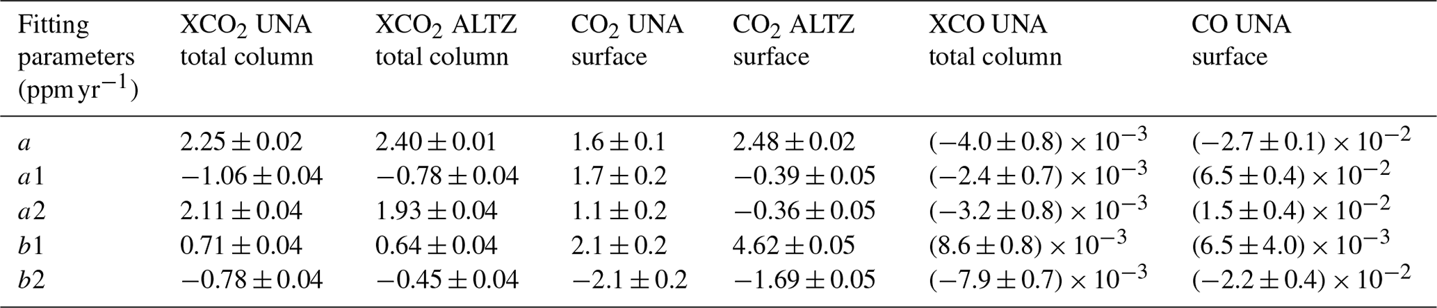
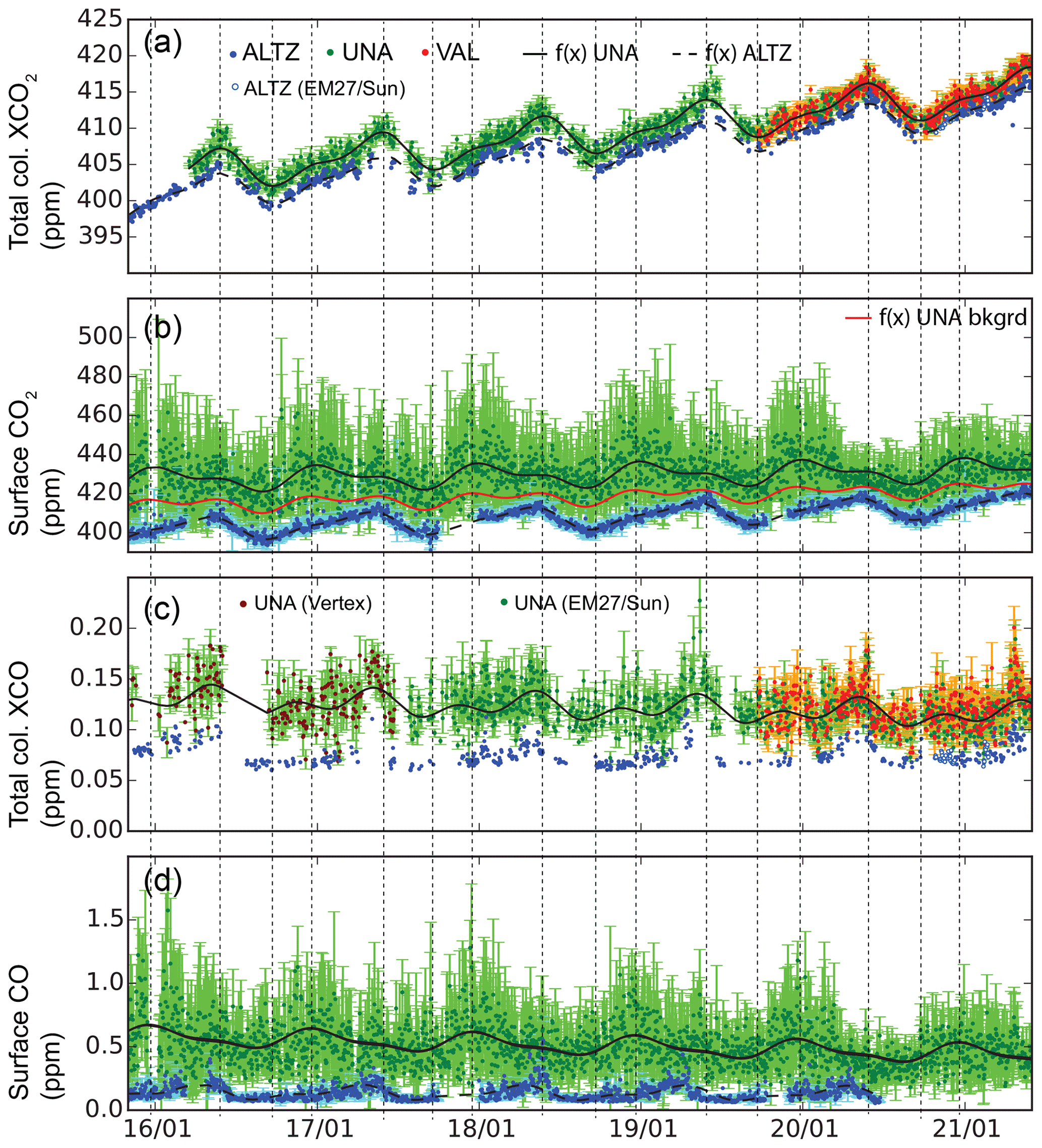
Figure 2 UNA (in green), VAL (in red) and ALTZ (in blue) time series of (a) the total column XCO₂ from the FTIR measurements, (b) the CO₂ surface concentration from the CRDS measurements, (c) the total column XCO from the FTIR measurements and (d) the CO surface concentration from the CRDS measurements. For each time series, the daily average data are presented as dots along with their daily standard deviations. Black traces show the annual fit calculated from the Fourier series (Eq. 7). In panels (a) and (c), we distinguish between ALTZ data obtained from the IFS120/5HR (blue full circles) and from the EM27/SUN (blue open circles); in panel (c), we distinguish between the CO total columns obtained from the VERTEX instrument (brown) and the EM27/SUN (green) at the UNA station. In panel (b), the red curve corresponds to the background fit, calculated following Gonzalez del Castillo et al. (2022), to determine the annual trend and seasonal cycles. The vertical dashed lines highlight the minimum and maximum of the annual cycles for the different products.

4 Results

The FTIR XCO₂ and XCO daily averaged time series and CO₂ and CO surface concentrations obtained at the UNA, VAL and ALTZ stations between November 2015 and June 2021 are shown in Fig. 2. Trends and seasonal variabilities were fitted using a Fourier series analysis (Eq. 7 and black and red solid lines in Fig. 2), following Wunch et al. (2013):

$$\begin{array}{}\text{(7)}& \begin{array}{rl}f\left(x\right)=& ax+{\sum }_{k=\mathrm{0}}^n{a}_{\mathrm{k}}\cos \left(\mathrm{2}\mathit{\pi }kx\right)+b_{\mathrm{k}}\sin \left(\mathrm{2}\mathit{\pi }kx\right),\\ & \text{ where }n=\mathrm{2}.\end{array}\end{array}$$

Here, x is the time (decimal year), a is the mean growth rate (ppm yr⁻¹), and a_k and b_k are the Fourier coefficients modulating the annual cycles. The coefficients for each gas species and station are reported in Table 3.

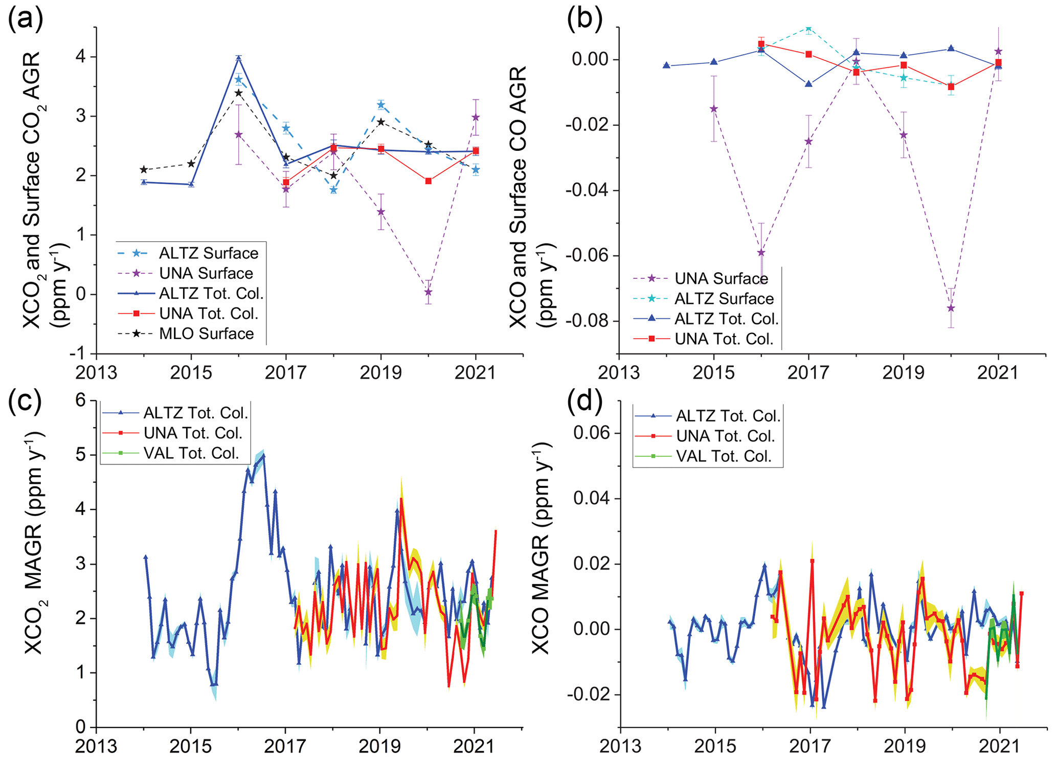
Figure 3 The XCO₂ (a) and XCO (b) annual growth rate (AGR) and XCO₂ (c) and XCO (d) monthly sampled annual growth rate (MAGR) obtained from total column and surface measurements for the UNA, VAL and ALTZ stations. In panel (a), the Mauna Loa (MLO) AGR trend is shown using a black dashed line. In panels (a) and (b), errors bars represent the standard error after removing annual cycles, reflecting the data sample quality. The standard error for the MAGR is shown as the shaded area in panels (c) and (d).

4.1 Trends and interannual variability

The total column XCO₂ time series (Fig. 2a) at ALTZ and UNA show a similar mean growth rate of around 2.4 ppm yr⁻¹ (2.4 and 2.3 ppm yr⁻¹ for ALTZ and UNA, respectively; Table 3) over the whole measurement period. A similar mean growth rate is also found for the surface CO₂ time series (Table 3 and Fig. 2b) at ALTZ (2.5 ppm yr⁻¹). These values are consistent with those estimated at the Mauna Loa Observatory (MLO) reference station for the 2016–2021 period (average of 2.5 ± 0.5 calculated from surface data available at the NOAA site: https://gml.noaa.gov/ccgg/trends, last access: 14 October 2024).

At UNA station, a surface mean growth rate of 1.6 ppm yr⁻¹ is found, which is lower than that observed from the total column measurements. Comparing the surface mean growth rates with those reported by González del Castillo et al. (2022) for the 2014–2019 period, we observe a significant difference for UNA station (2.3 ppm yr⁻¹ in González del Castillo et al., 2022) but very similar values for the ALTZ station (2.6 ppm yr⁻¹ in González del Castillo et al., 2022). The difference observed at UNA station could stem from (i) starting our new time series at the end of 2015, when the annual growth rate was highest (González del Castillo et al., 2022), and (ii) the inclusion of the 2019–2021 period, when the mean growth rate clearly decreased. At VAL station, the total column XCO₂ time series are found to be very similar to those observed at UNA station (Fig. 2a). Figure S1 in the Supplement shows that 86 % of the daily average data at VAL and UNA have a difference lower than 1.0 ppm, although a large part of the comparison was done during the COVID-19 lockdown period (Table 1), when lower gradients are expected due to the decrease in the anthropogenic emissions.

According to Buchwitz et al. (2018), the interannual variability can be explored through the time series of the mean annual growth rate (AGR) and the monthly sampled annual growth rate (MAGR). The MAGR is calculated by month, as the difference between the monthly averaged Xgas data of a year i and the monthly averaged data of the previous year (i−1). The AGR is obtained for each year, averaging all of the MAGR values. The AGR and MAGR values for total column and surface measurements are presented in Fig. 3. We include data from the MLO in Fig. 3a, for which the AGR (dashed black curve) was derived from the surface data available at the NOAA site.

At ALTZ, the interannual variability in the total column XCO₂ AGR (Fig. 3a) was found to be similar to that obtained from both the ALTZ and MLO surface data, with a coincident peak in 2016, reaching an AGR value of 3.5ppm yr⁻¹ (surface data) and 4.0ppm yr⁻¹ (total column data). Surface data AGR time series show a second peak in 2019, which is not apparent in the total column XCO₂ time series. The time series of the MAGR (Fig. 3c) allows for better identification and characterization of the period and duration of the anomalies. The 2016 XCO₂ anomaly has a duration of up to 15 months (from October 2015 to March 2017), reaching a maximum value (around 5.0 ppm yr⁻¹) between March and July 2016, corresponding to a factor of 2.8 higher than the 2013–2015 base level (1.8 ppm yr⁻¹).

At UNA, the XCO₂ AGR and MAGR time series (Fig. 3a and c) are very similar to those observed at ALTZ station, except for the year 2020. During this year, the AGR dropped by ∼ 20 % at UNA before returning to the level of the previous 2 years in 2021. This behaviour contrasts with the AGR observed at ALTZ, which remains nearly constant between 2017 and 2021. The MAGR time series at UNA (Fig. 3c) shows that this drop is dominated by the exceptionally low June and October growth rates, representing the lowest MAGR values of the UNA time series. This observation is supported by the VAL MAGR, although the time series is much shorter. The surface CO₂ AGR at UNA shows a much higher interannual variability, with the strongest anomaly observed in 2020, where the AGR is close to zero. A very clear decrease in the day-to-day and intraday CO₂ surface variability is observed in Fig. 2b from April to mid-September 2020, consistent with the XCO₂ MAGR anomaly.

Upon examination of CO, the UNA XCO time series (Fig. 2c) has daily averages ranging between 0.10 and 0.23 ppm with a mean and standard deviation of 0.12 and 0.02 ppm, respectively, but it shows a decreasing rate (−4.0 × 10⁻³ ppm yr⁻¹) over the whole measurement period. The VAL XCO time series show a very similar baseline to UNA, with a daily average difference lower than 0.02 ppm for 85 % of the coincident dataset (Fig. S1). At the ALTZ background site, the XCO baseline and day-to-day variability are lower than at UNA and VAL (mean and standard deviation equal to 0.08 and 0.01 ppm, respectively), as expected. The surface CO time series (Fig. 2d) shows a more significant decreasing trend (−2.7 × 10⁻² ppm yr⁻¹) than the total column data at UNA, while the baseline at ALTZ remains constant at around 0.11 ppm. The XCO and CO AGR and MAGR at ALTZ and UNA are shown in Fig. 3b and d. Generally, the XCO AGR and MAGR oscillate around their base level at the ALTZ and UNA stations, with short-term anomalies. At ALTZ, a strong negative XCO AGR anomaly is observed in 2017, which was not observed for XCO₂, likely resulting from the exceptionally high XCO columns measured during 2016. This is supported by the increase in the XCO MAGR from October 2015 to July 2016 (Fig. 3d), coinciding with the first 10 months of the highest XCO₂ anomaly and followed by the lowest XCO MAGR values of the time series (around −0.02 ppm yr⁻¹ in April 2017). At UNA station, the XCO AGR slightly decreases between 2016 and 2020 and increases again in 2021. The most significant and prolonged (> 5 months) MAGR anomaly (Fig. 3d) occurred between April and September 2020, with negative values. Some short-term additional anomalies are observed, but only a few of them (in May 2018 and January 2019) are not affected by the limited number of available measurements.

4.2 Seasonal variability and short-term cyclic events

Annual cycles are observed for both total column XCO₂ and CO₂ surface measurements at ALTZ, UNA and VAL stations (Fig. 2). The maximum and minimum values of the total column XCO₂ cycles are observed in May–June and September, respectively, with an average amplitude of around 5 (ALTZ) and 6 (UNA) ppm.

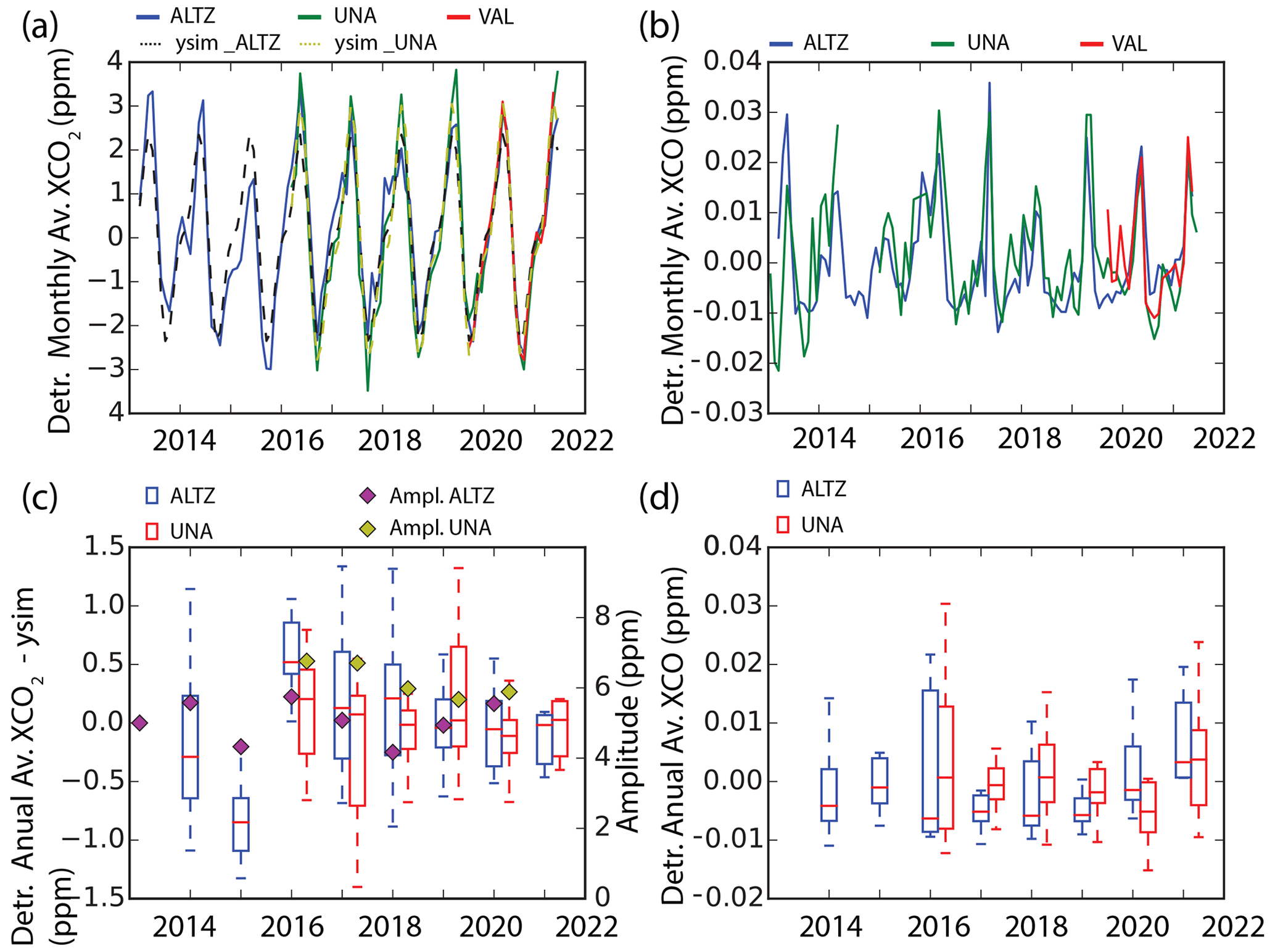
Figure 4 Interannual and annual variability in the detrended XCO₂ and XCO total column data at the UNA, VAL and ALTZ stations. In panel (a), the dash line represent the detrended mean annual cycle. In panels (c) and (d), the whisker diagrams are calculated from the monthly average detrended data. The amplitude is determined as the max–min values.

To examine the temporal changes in the amplitude and shape of the annual cycles, total column data were monthly averaged, detrended by subtracting the linear part of the fit (f(x) = ax; Eq. 7) and compared to the detrended mean annual cycle (f(x)−ax; in Fig. 4). To obtain a longer-term view, we included the 2013–2015 period from ALTZ station, previously published in Baylon et al. (2017), after applying the intercalibration factors (Sect. 3.1.3). At ALTZ, two periods significantly deviated from the average XCO₂ seasonal cycle, i.e. (i) the year 2015, when all of the monthly averaged XCO₂ values are below the fit and one of the lowest seasonal amplitudes (∼ 4.0 ppm; Fig. 4a and c) of the whole time series is observed, and (ii) the year 2016, when higher monthly averages than the mean XCO₂ seasonal cycle are found and the highest amplitude (∼ 5.8 ppm; Fig. 4a and c) is observed. At UNA, the difference with respect to the average XCO₂ seasonal cycle is not significant, except for the year 2020, when all of the monthly averages are below the mean annual cycle (Fig. 4c). During this period, the UNA and VAL XCO₂ monthly averaged data fit exceptionally well with those of ALTZ station between March 2020 and March 2021 in terms of the shape and amplitude, while the UNA and VAL annual cycle amplitudes are slightly higher than those of ALTZ for the other years.

Regarding the CO₂ surface data (Fig. 2b), annual cycles are observed, with maxima and minima reached in mid-December and mid-September, respectively. As also reported in González del Castillo et al. (2022), the maximum occurred during winter, when a shallower boundary layer prevailed, and the summer–autumn minimum can be explained by the dilution of trace gases in a deeper convective boundary layer and more active urban vegetation.

XCO peaks at the three stations in April–May every year (Figs. 2c and 4b) and then shows minimal annual values in August, preceding the minimum and maximum values of the XCO₂ time series by 1 month. The April–May maximal annual values, also confirmed by TROPOMI measurements (Borsdorff et al., 2020), coincide with the biomass-burning season and the periods during which the mixed layer reaches its maximum altitude (García-Franco et al., 2018). During 2015, the XCO time series show a very low maximum reached in February instead of May (Fig. 4b), contrasting with 2016, when high total column XCO values are reached in January and maintained for a period of at least 5 months. The year 2016 also corresponds to the period with the highest XCO variability in the time series (Fig. 4d). Additionally, in 2018, the XCO annual cycles differ from the other years, with lower values and a flat shape during the first semester of the year (January–May).

Surface CO data (Fig. 2d) also show periodic increases at ALTZ station with maxima reached during April–May, coinciding with the maxima observed from total column XCO measurements. They confirm the increase in the CO emissions during the biomass-burning season, which is at least dominant in the ALTZ measurements. However, at UNA station, although they are observed in the surface data, cycles have a maximum coinciding with that of the CO₂ surface data and lag behind the XCO total columns. These cycles are likely dominated by other processes affecting both CO and CO₂ species, such as the mixed-layer seasonal dynamic.

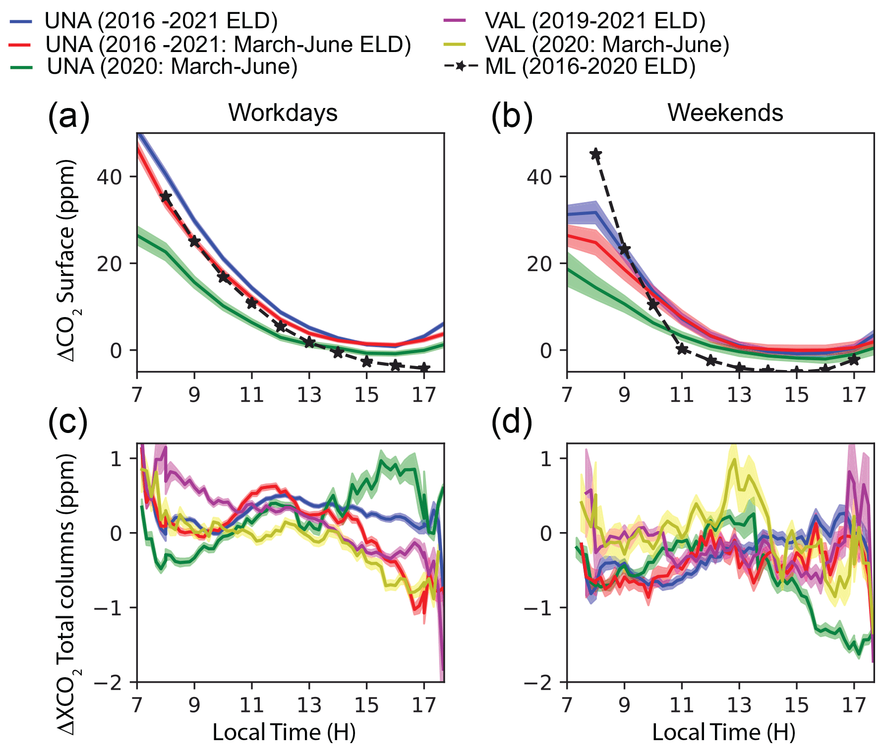
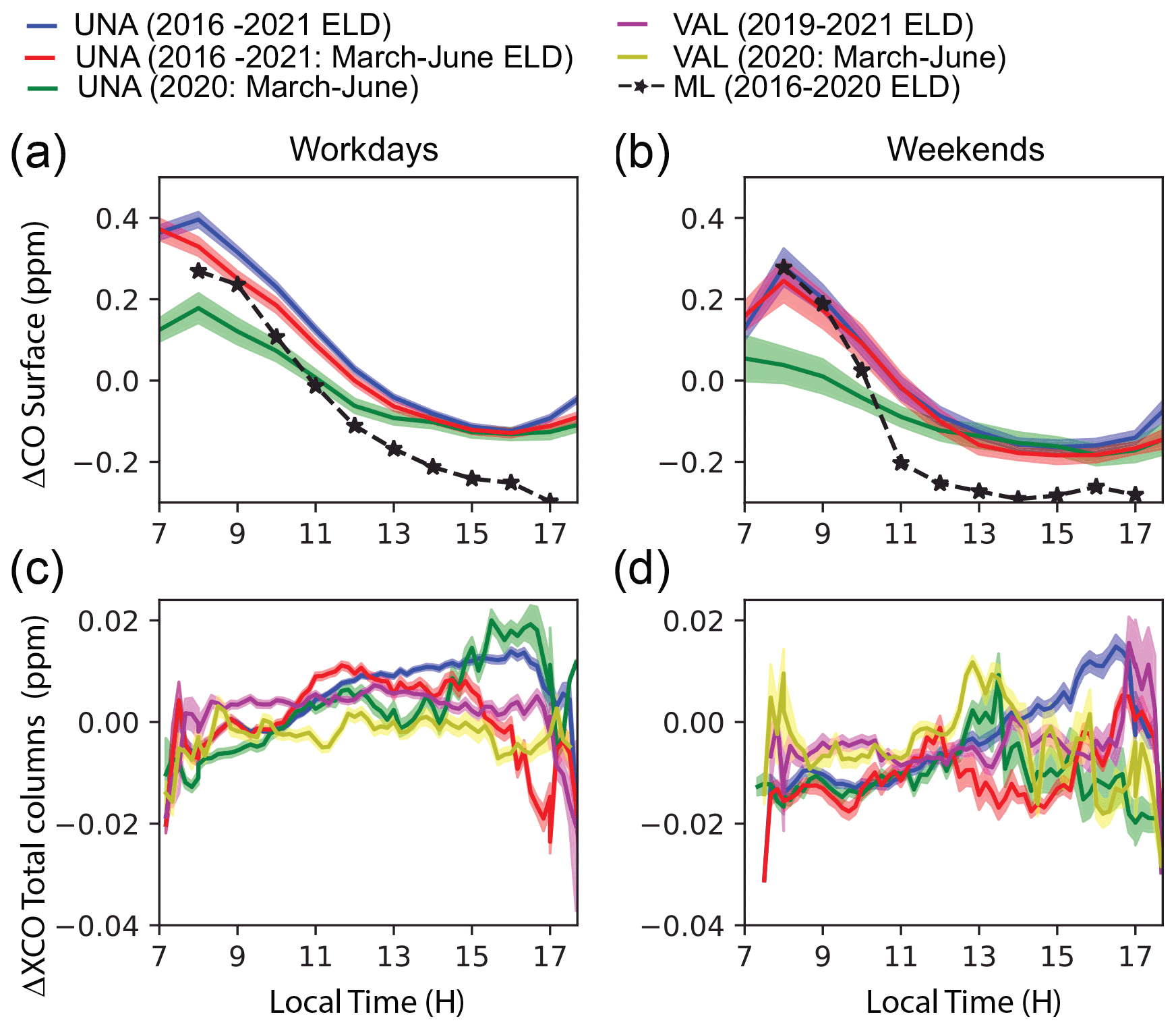
Figure 5 Diurnal patterns in the detrended surface CO₂ mole fractions (a, b) and XCO₂ total columns (c, d) measured at the UNA and VAL stations. For each panel, the different curves represent different time periods: blue denotes the whole measurement period excluding the lockdown (March–June 2020) period, green denotes the lockdown period (March–June 2020), and red denotes the whole measurement period including only the March to June months but excluding the lockdown period. The standard errors are presented as shaded areas. Black curves represent the diurnal pattern of CO₂ in the mixed layer (ML) calculated from the total column data for UNA station.

4.3 Intraday variability

The intraday variability in the total columns and surface data is depicted in Figs. 5 and 6. As the ALTZ total column data do not present a significant diurnal pattern (the hourly variability remains lower than the standard error of the time series), they are not presented in these plots.

Total column data were detrended by removing the seasonal fit (black traces in Fig. 2a and c) and were averaged over 10 min. To avoid a possible bias due to strong ventilation periods, a filter based on a ventilation index (VI) was applied, following the recommendations in Hardy et al. (2001), Su et al. (2018), and Storey and Price (2022). The VI is calculated as the product of the average wind speed velocity (between the surface and 100 m height) and the planetary boundary layer (PBL) height for the UNA and VAL locations. The wind velocity and the MLH were estimated from the hourly ERA5 reanalysis products (wind components and PBL height fields) (Hersbach et al., 2020). In the MCMA, the surface wind speed presents a diurnal pattern, generally reaching a maximum during the afternoon between 14:00 and 15:00 LT (Fig. S4). The filter selects the days complying with the following criteria: (i) a maximum wind velocity (average 10–100 m height) between 10:00 and 12:00 LT that is lower than 1.5 m s⁻¹ (threshold based on Stremme et al., 2013) and (ii) a daily VI lower than 2350 m² s⁻¹, which represents a commonly used threshold for selecting poor ventilation conditions (Hardy et al., 2001; Storey and Price, 2022). About 60 % of the original XCO₂ and XCO dataset is selected by applying the filter, and this subset will be considered in the following analysis. We note that about 70 % of the discarded data points correspond to the January–May period of the year. Filtered total column XCO₂ and XCO data were averaged over 10 min and are presented in panels (c) and (d) in Figs. 5 and 6, distinguishing between the workday (WD) and weekend (WE) periods. To explore the 2020 lockdown influence on the diurnal pattern, three different periods are shown in each plot: the first period (blue curve: 2016–2021) refers to the whole measurement period excluding the interval between March and June 2020, corresponding to the lockdown period (hereafter called “ELD” to denote that it excludes the lockdown period), where a significant MAGR decrease was observed; the second period (green curve: March–June 2020) refers to the lockdown period but excludes the rainy season to avoid bias due to incomplete daily time series; and the third period (red trace) is the same as the first one but only considers the March–June months to be compared with the lockdown period.

Figure 6 The same as Fig. 5 but from surface CO and total column XCO measurements.

Surface data from the CRDS analysers were detrended by removing the background fit, following the methodology described in the Sect. 3.2, and filtered to be coincident with the filtered total column measurements (selection of data between 07:00 and 18:00 LT, only including the days with low-ventilation conditions). They were finally averaged by hour and are presented in panels (a) and (b) in Figs. 5 and 6 for the WD and WE periods, respectively, for which each curve represents the periods mentioned above.

The surface CO₂ diurnal pattern at UNA station for the whole measurement period (2016–2021; blue curves Fig. 5a and b) is consistent with that previously described in González del Castillo et al. (2022) for the 2014–2019 period, with a maximum observed during the early morning (reached before 07:00 LT), a minimum during the afternoon (between 15:00 and 16:00 LT) and an average amplitude of around 45 ppm. A lower amplitude of these cycles is observed during the WE (average amplitude of 28 ppm) with respect to the WD periods. During the 2020 lockdown period (green curve), the WD surface CO₂ diurnal profile has a comparable amplitude (average amplitude of 26 ppm) to that of the WE for the whole measurement period, but it is slightly higher than that observed during the lockdown WE periods (average amplitude of 22 ppm). The surface CO diurnal profile (2016–2021; blue curve in Fig. 6) peaks at 08:00 LT and then decreases until 16:00 LT during any day of the week. The WD and WE data show amplitudes of up to 0.5 ppm and 0.3 ppm, respectively. During the lockdown period, the WD and WE amplitudes are much lower (0.3 and 0.2, respectively), consistent with the CO₂ surface observations.

The XCO₂ and XCO diurnal patterns (panels c and d in Figs. 5 and 6) have very different shapes compared with those of the surface data, with amplitudes 1 order of magnitude lower. The variability observed between 07:00 and 08:00 LT is likely due to the low number of measurements during this time interval; thus, it will not be taken into account in the following analysis. The UNA and VAL XCO₂ diurnal patterns significantly differ with respect to shape. The VAL WD curve (magenta) continuously decreases from 08:00 to 17:00 LT (amplitude of around 2 ppm) during both the whole measurement and lockdown periods; however, during the lockdown period, lower values are generally recorded, with higher intra-hour variability between 11:00 and 14:00 LT. The general WD decreasing trend suggests that a maximum is reached during the early morning (before 07:00 LT). This observation is supported by the CO₂ surface measurements performed with the low-cost, medium-precision CO₂ sensors (Porras et al., 2023), recording a maximum between 06:00 and 07:00 LT. The UNA XCO₂ WD diurnal pattern (blue trace) is almost constant until 10:00 LT; it then increases until it reaches a maximum at around 12:00 LT, slightly decreases until 17:00 LT and finally shows an abrupt decrease after that. The amplitude of the diurnal variability is around 1 ppm. During the lockdown period, the diurnal profile is different: it increases until 12:00 LT, slightly decreases until 13:00 LT, increases again until it reaches a maximum at 16:00 LT and then finally abruptly decreases until 17:00 LT. The lockdown WD XCO₂ profile shows lower values than the other periods until 13:00 LT, but the peak observed at 16:00 LT is not apparent for the other periods. Variability is generally lower during the WE (< 1 ppm), except for the lockdown period, for which an important decrease is observed after 14:00 LT, but it is likely affected by the low number of measurement days. For XCO, the diurnal profiles also have different shapes at UNA and VAL. At UNA, the March–June XCO diurnal profiles (red and green curves) resemble those of XCO₂ for both the lockdown and whole measurement periods. When considering the 12 months of the year (blue trace), the maximum curve slightly increases between 12:00 and 16:00 LT, when it reaches its maximum. This contrasts with the variability in the March–June curves during this time interval, for which an increase is observed when considering the lockdown period and a decrease is observed when considering the whole measurement period. At VAL, the diurnal profile is fairly constant until 17:00 LT, with slightly lower values during the lockdown period.

The total column XCO diurnal profiles during the WE are less reliable, with larger standard errors, likely due to the low number of considered measurements. Nevertheless, an increase is observed at UNA, where the considered day's number is statistically more reliable, with a peak at around 17:00 LT, which was not observed for XCO₂.

The difference observed between the diurnal pattern of XCO and XCO₂ at VAL and UNA is likely due to the different advection drivers in the region, which are mainly controlled by the topography. A northern surface wind direction (Fig. S6) is generally dominant over the Basin of Mexico, but it is locally highly influenced by mountainous barriers. The west-northwest wind component at UNA is likely to be the effect of downslope flows from the mountain ridge in the early morning (mostly between 06:00 and 09:00 LT). In contrast, at VAL, the plateau-to-basin winds are the main influx into the basin coming from the northwest in the morning. There can also be an influence from an up-valley flow in the mornings (de Foy et al., 2006). More generally, VAL station is likely influenced by the northern mountain, generating a significant gradient in the CO distribution upwind of the station (Fig. 1). In contrast, near UNA station, the flat ground allows more efficient mixing and, due to the dominant north-northeast wind component in the late morning, the captured air masses likely often reflect the MCMA plume emissions.

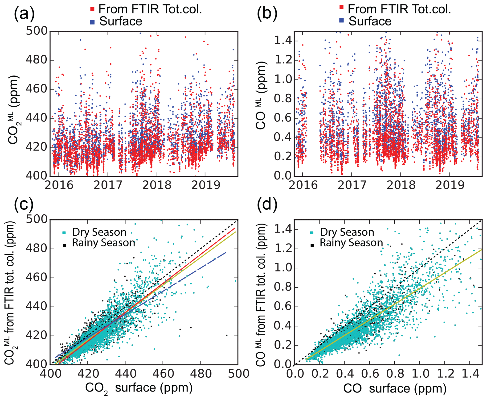
Figure 7 Comparison between (a) the ${\mathrm{CO}}_{\mathrm{2}}^{\mathrm{ML}}$ and (b) CO^ML products derived from the ALTZ and UNA total column measurements (red) and the surface measurements (blue) at UNA station. Panels (c) and (d) represent the correlation plots for CO₂ and CO, respectively. In panels (c) and (d), we distinguish between data corresponding to the dry (November–May: cyan) and rainy (June–October: black) seasons. In panel (c), the yellow, red and blue linear regression curves correspond to the whole measurement period (yellow: slope = 0.95 ± 0.02; offset = 17.9 ± 0.2; R² = 0.74), the dry season (red: slope = 1.00 ± 0.02; offset: −2.9 ± 0.2; R² = 0.77) and the rainy season (blue: slope = 0.80 ± 0.03; offset: 83.7 ± 0.39; R² = 0.66). In panel (d), as no significant difference was found for the different periods, the regression lines (yellow: slope = 0.81 ± 0.02; offset: −0.021 ± 0.004; R² = 0.74) represent the whole measurement. The black dashed line represents y=x.

4.4 CO and CO₂ within the mixed layer from FTIR and surface data

Figure 7 shows the hourly averaged CO₂ and CO concentration within the mixed layer (${\mathrm{CO}}_{\mathrm{2}}^{\mathrm{ML}}$ and CO^ML products, respectively), calculated from the FTIR measurements (see Sect. 3.3), as well as the surface data. The ${\mathrm{CO}}_{\mathrm{2}}^{\mathrm{ML}}$ and CO^ML products are in agreement with the surface observation, with a slope of 0.95 ± 0.02 (R² = 0.74) for CO₂ (Fig. 7c) and 0.81 ± 0.02 (R² = 0.74) for CO (Fig. 7d). For CO₂, the slope was found to be closer to 1.0 (1.00 ± 0.02), with an offset of −2.9 ± 0.2 and a better R² (0.77), when discarding the data corresponding to the rainy season. This effect is likely due to the removal of the incomplete daily time series that was frequently interrupted in the early afternoon during the rainy season.

The ${\mathrm{CO}}_{\mathrm{2}}^{\mathrm{ML}}$ and CO^ML diurnal patterns are presented in panels (a) and (b) in Figs. 5 and 6 (dashed lines) along with those of surface measurements, after similar filtering. The ${\mathrm{CO}}_{\mathrm{2}}^{\mathrm{ML}}$ and surface CO₂ diurnal patterns (Fig. 5a and b) are very similar with respect to shape and amplitude, especially during the WD period, although a small difference is observed in the late afternoon (< 5 ppm). This difference is likely due to the increase in the uncertainties of the MLH estimate when it is more diluted. The CO^ML and surface CO diurnal profiles (Fig. 6a and b) also have similar amplitudes and shapes for both the WD and WE periods, although the CO^ML diurnal profile shows lower values (offset of around 0.1 ppm for WD). Despite this very simplified model, these results show that the total column and surface measurements are mutually very consistent when the seasonal and diurnal variability in the mixed-layer expansion above Mexico City is taken into account.

4.5 XCO / XCO₂ enhancement ratios

The correlated XCO and XCO₂ enhancements and their ratio can give insights into the combustion efficiency of the sources in a city and, therefore, into their contributions. In this study, we explored the variability in the XCO / XCO₂ ratios at both long-term and intraday scales.

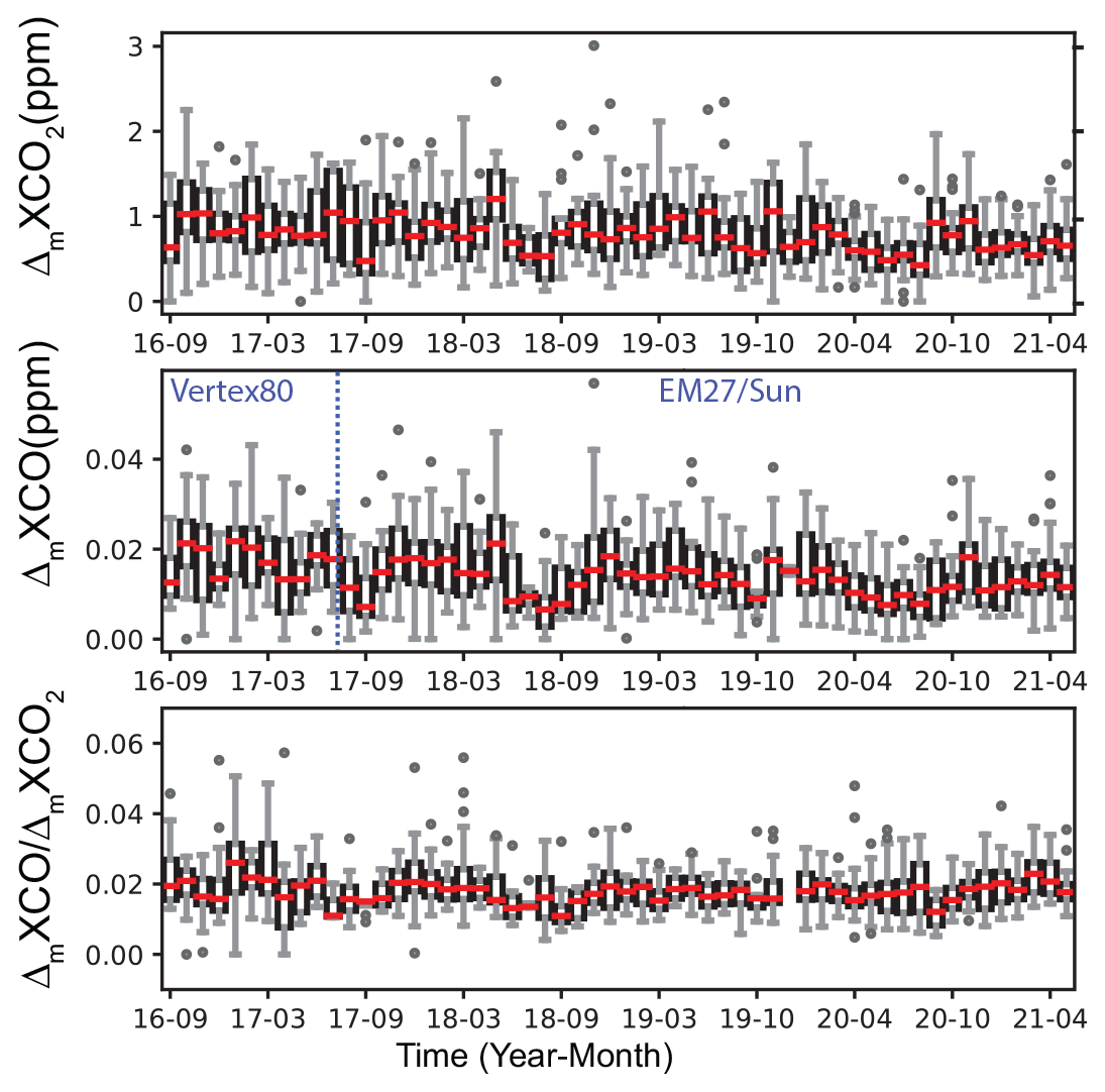
Figure 8 Whisker diagram representing the month-by-month variability in ΔXCO₂, ΔXCO and their ratio from the UNA measurements.

For the long-term analysis, the XCO₂ “background” level was calculated using a statistical method, employing the lower 5th percentile of the measured Xgas over a 1 d running window (You et al., 2021). We did not use the ALTZ measurements because of (i) the periodic influence of wildfires in the region during the dry season and (ii) the discontinuity of our daily averaged time series. The enhancements of XCO₂ and XCO above background (Δ_mXCO₂ and Δ_mXCO, respectively) measured at UNA are presented in Fig. 8, as whisker diagrams.

Both the Δ_mXCO₂ and Δ_mXCO time series show a slight decrease over time (around 0.05 and 0.001 ppm yr⁻¹, respectively). Although the ${\mathrm{\Delta }}_{\mathrm{m}}\mathrm{XCO}/{\mathrm{\Delta }}_{\mathrm{m}}{\mathrm{XCO}}_{\mathrm{2}}$ ratio displays variability around its mean value (0.018 ± 0.003), there are no discernible cyclic or long-term trends in the time series, except for the rainy periods of 2017, 2018 and 2020 when low ratios (and low Δ_mXCO and Δ_mXCO₂ values) were observed. The Δ_mXCO and the ${\mathrm{\Delta }}_{\mathrm{m}}\mathrm{XCO}/{\mathrm{\Delta }}_{\mathrm{m}}{\mathrm{XCO}}_{\mathrm{2}}$ ratio show higher variability at the beginning of the time series (until July 2017), likely due to the use of the CO VERTEX products. The long-term Δ_mXCO decrease, also observed in other studies (García-Franco, 2020; Molina, 2021; Hernández-Paniagua et al., 2021), likely reflects the effect of the successive air quality management programmes implemented in the MCMA since the 1990s, including technological advancements and fuel quality enhancements as well as refinery closures, industrial relocation or fuel substitution. Regarding the low seasonal variability observed in the $\mathrm{CO}/{\mathrm{CO}}_{\mathrm{2}}$ ratios, this is likely related to biomass-burning episodes and high-pressure weather conditions that occur during the dry season.

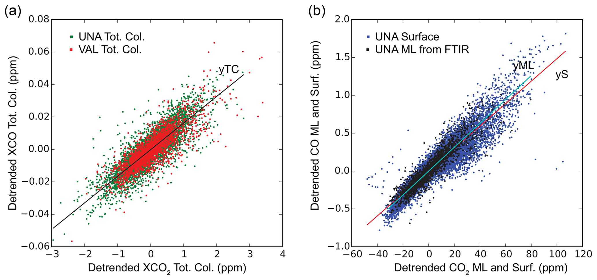
Figure 9 Correlation plot of (a) the detrended (by removing the daily averages) hourly average total column XCO vs. XCO₂ data as well as (b) the detrended hourly average mixed-layer (ML) and surface CO vs. CO₂ products. Solid lines represent the linear regression lines, with the following parameters: TC slope = 0.0164 ± 0.0003 and R² = 0.72 for the total columns at UNA and VAL, yS slope = 0.0148 ± 0.0001 and R² = 0.87 for the surface products, and yML slope = 0.0158 ± 0.0002 and R² = 0.88 for the mixed-layer products.

To perform the intraday analysis, the hourly averaged data were detrended by subtracting the daily average. The resulting ΔXCO₂ vs. ΔXCO datasets are plotted in Fig. 9a. The entire ΔXCO₂ and ΔXCO datasets show a good correlation at both the UNA and VAL stations, with similar linear regression slopes of around 0.0164 ± 0.0003, which is consistent with that found from the surface measurements and the mixed-layer product (Fig. 9b). Although there is an actual difference in the emission types in the southern and northern parts of the city, with the north hosting industrial and commercial sources and the south being largely residential and commercial, the common and dominant source of CO in the MCMA (at the UNA and VAL stations) is believed to be motorized vehicles. The data dispersion around the regression line likely reflects a shorter-term and more local influence from other sources with an important week-to-week variability.

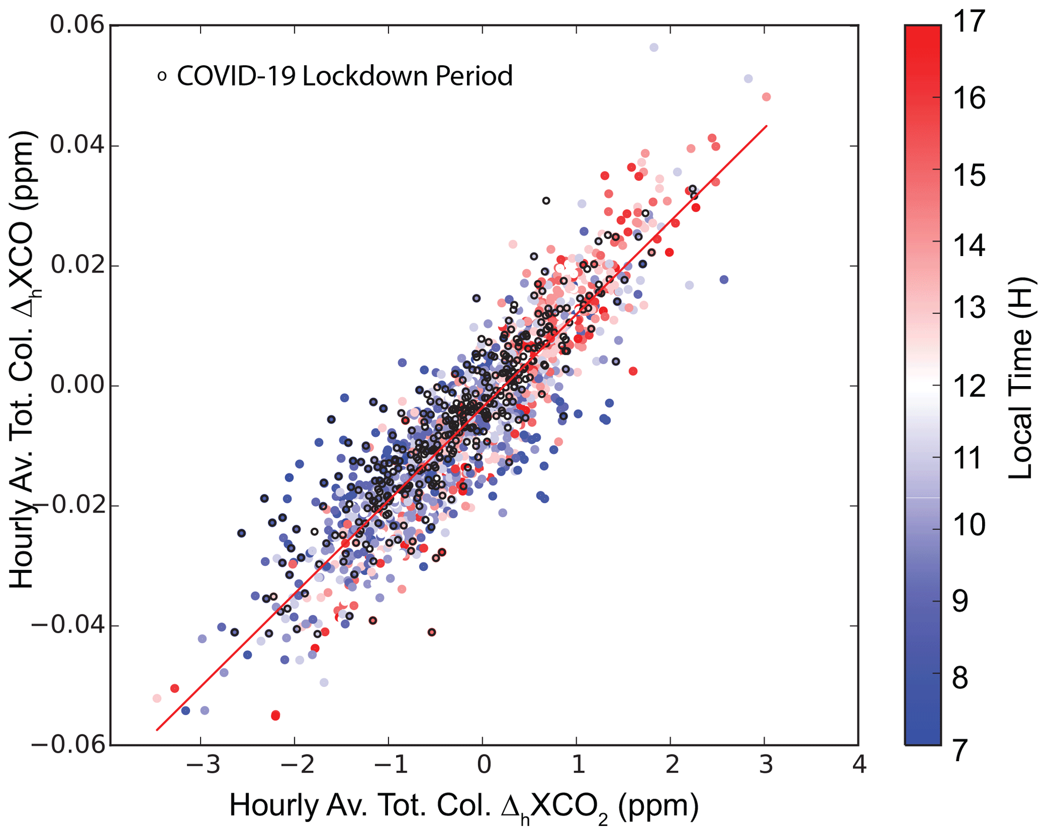
Figure 10 Correlation plot of the ΔXCO (UNA − VAL) vs. ΔXCO₂ (UNA − VAL) hourly averages (colour scale with respect to time is shown to the right) for the coincident measurement period (September 2019–June 2021). Dots with black outlines highlight the measurements during the COVID-19 lockdown period (March–June 2020). With respect to the regression line (in red), slope = 0.015 ± 0.001 and R² = 0.80.

On the other hand, the total column (UNA − VAL) differences (presented in Fig. S3) can also be used to calculate the $\mathrm{\Delta }\mathrm{XCO}/\mathrm{\Delta }{\mathrm{XCO}}_{\mathrm{2}}$ ratio, with a more precise subtraction of a common background (which assumes a homogeneous background across the entire city) from the two stations. Figure 10 shows the hourly average ΔXCO₂ (UNA − VAL) vs. ΔXCO (UNA − VAL) correlation plot for the coincident measurement period. A well-defined linear correlation is observed with a slope of 0.015 ± 0.001 and a coefficient of determination of R² = 0.80, highly consistent with the findings displayed in Fig. 9. The use of the (UNA − VAL) total column difference notably improved the coefficient of determination, by removing the regional long-term and short-term perturbations affecting the two sites. The intraday variability in the ΔXCO (UNA − VAL) / ΔXCO₂ (UNA − VAL) ratio (colour scale in Fig. 10), showing higher columns at VAL during the morning and at UNA during the afternoon, likely reflects the north-to-south transport of air across the city. We note that the ratio remains the same during the lockdown period. We would expect lower intraday (UNA − VAL) ΔXCO and ΔXCO₂ amplitudes during the lockdown period, but this is not clearly apparent in this correlation plot.

4.6 Estimate of CO and CO₂ MCMA emissions

The variability in the long-term CO emissions in the MCMA can be estimated following the method detailed in Stremme et al. (2013). In the aforementioned study, they assumed that, as the CO emissions in the MCMA are mainly due to traffic pollution, the rapid changes observed in the CO total column should reflect the fresh CO emissions under certain meteorological conditions. Low ventilation, strong turbulence in the mixed layer and a limited zenithal angle of measurements are critical criteria to avoid enhancement due to horizontal transport or local heterogeneity. CO total column growth rates can be estimated at specific time intervals complying with these conditions from long-term time series. Further details on the method and the estimation of uncertainties due to these assumptions are given in Stremme et al. (2013). Here, we determined an optimized time interval for estimating the mean CO growth rate using (i) the diurnal surface wind speed patterns and (ii) the diurnal MLH growth rate, with the latter reflecting the turbulence within the mixed layer (Fig. S4). The time interval complying with rapid growth of the mixed layer and a low surface wind speed (< 2 m s⁻¹) was found to be between 10:00 and 12:00 LT, which is in agreement with the requirements mentioned in Stremme et al. (2013). CO growth rates and their uncertainties were determined by year, based on the linear regression (with 95 % confidence interval) of the 10 min average detrended CO total columns over the 10:00–12:00 LT interval. For example, for the year 2018, we found a CO growth rate of 52 ± 5 kg km⁻² h⁻¹.

To extrapolate the growth rate over the MCMA, we used the TROPOMI CO total column data that we averaged over the 2018–2022 period (Fig. 1), following the same method as described in Stremme et al. (2013). We assume that the total amount of fresh CO is proportional to the total emissions in the MCMA and to the total column enhancement at the UNA site, which reflects the CO accumulated at this site. The ratio of the total accumulated CO in the MCMA to the columnar CO at UNA is, therefore, the same ratio as the total emissions of the whole megacity to the UNA emission flux, in units of molecules per area per unit time. Thus, this ratio is the extrapolation factor and represents an effective area, defined as follows:

$$\begin{array}{}\text{(8)}& \mathrm{Effective}\mathrm{\_}\mathrm{area}={\displaystyle \frac{\stackrel{\mathrm{MCMA}}{\int }\left(\mathrm{CO}(A{)}_{\mathrm{MCMA}}-{\mathrm{CO}}_{\mathrm{bgrd}}\right)dA}{{\mathrm{CO}}_{\mathrm{UNA}}-{\mathrm{CO}}_{\mathrm{bgrd}}}}.\end{array}$$

Here, the term (CO_MCMA−CO_bgrd) is integrated over the area in which the CO TROPOMI total columns are higher than a predefined background value. As the TROPOMI overflight time is around 13:30 LT, we cannot neglect the fact that ventilation and slight advection is smoothing out the distribution; therefore, both the background and the column at UNA have to be chosen carefully. Thus, the background column was estimated in two ways: (i) from the smallest value observed upwind of the city (cross symbol in Fig. 1) at the elevation of the Basin of Mexico (contour line separating Mexico City from the Toluca area in the west in Fig. 1), which was found to be 1.45 × 10¹⁸ $\mathrm{molec}.{\mathrm{cm}}^{-\mathrm{2}}$, and (ii) from the Tecámac site (where the border of the MCMA was assumed to be in Stremme et al., 2013), which was found to be 1.60 × 10¹⁸ $\mathrm{molec}.{\mathrm{cm}}^{-\mathrm{2}}$.

Due to advection, even locations slightly outside of the megacity present enhanced CO columns; thus, the actual background column in the Basin of Mexico is unclear. Figure S5 illustrates the sensitivity of the effective area to the background uncertainties. A 10 % higher background leads to a 40 % smaller extrapolation factor and a 40 % emission underestimate. Fresh CO was estimated from the TROPOMI data by removing the background (1.45 × 10¹⁸ $\mathrm{molec}.{\mathrm{cm}}^{-\mathrm{2}}$) from the average total columns found at UNA (1.93 × 10¹⁸ $\mathrm{molec}.{\mathrm{cm}}^{-\mathrm{2}}$) and was found to be 4.79 × 10¹⁷ $\mathrm{molec}.{\mathrm{cm}}^{-\mathrm{2}}$. In cases in which the CO total column is lower than the background, likely due to the topography effect, we set the difference column to zero for the integration. This topographic effect is important for the considered area, as there are plenty of mountains around the basin, including the mountain ridge to the west (e.g. Ajusco and Desierto de los Leones), some mountains to the east, and the Popocatépetl and Iztaccíhuatl volcanoes to the south.

Finally, we found effective areas of ∼ 2017 km² (outer area, blue contour line in Fig. 1) and ∼ 1178 km² (inner area, red contour line in Fig. 1) considering the two background values given above. The inner area reflects conditions without a ventilation effect; therefore, the outer area is more appropriate for the emission estimates, given that the TROPOMI measurements occurred at 13:30 LT and ventilation at this time cannot be neglected. Hereafter, the other estimates calculated from the inner area will only be indicated within parentheses and are considered to estimate the sensitivity of the result.

As the measured growth rate corresponds to a time interval of only 2 h in the middle of the day, the CO intraday fluctuations have to be taken into account. Stremme et al. (2013) used a factor that was taken from the available bottom-up inventories and described that the CO emissions per day are roughly 18.5 times the emission per hour at noon. Assuming the same factor, we estimate a CO rate of around 0.71 ± 0.06 (0.42 ± 0.04) Tg yr⁻¹ for 2018. If no information about the diurnal distribution of the emission rate is available, we should assume a uniform distribution, and an upper CO rate value could be estimated using an intraday time interpolation factor of 24 h instead of 18.5 h, finally resulting in ∼ 30 % higher estimates. Despite the significant uncertainties introduced by spatial and temporal interpolation, their impact on the relative variability, trends and anomalies of the emission rates is less important if the same method and assumptions are consistently applied across the entire time series.

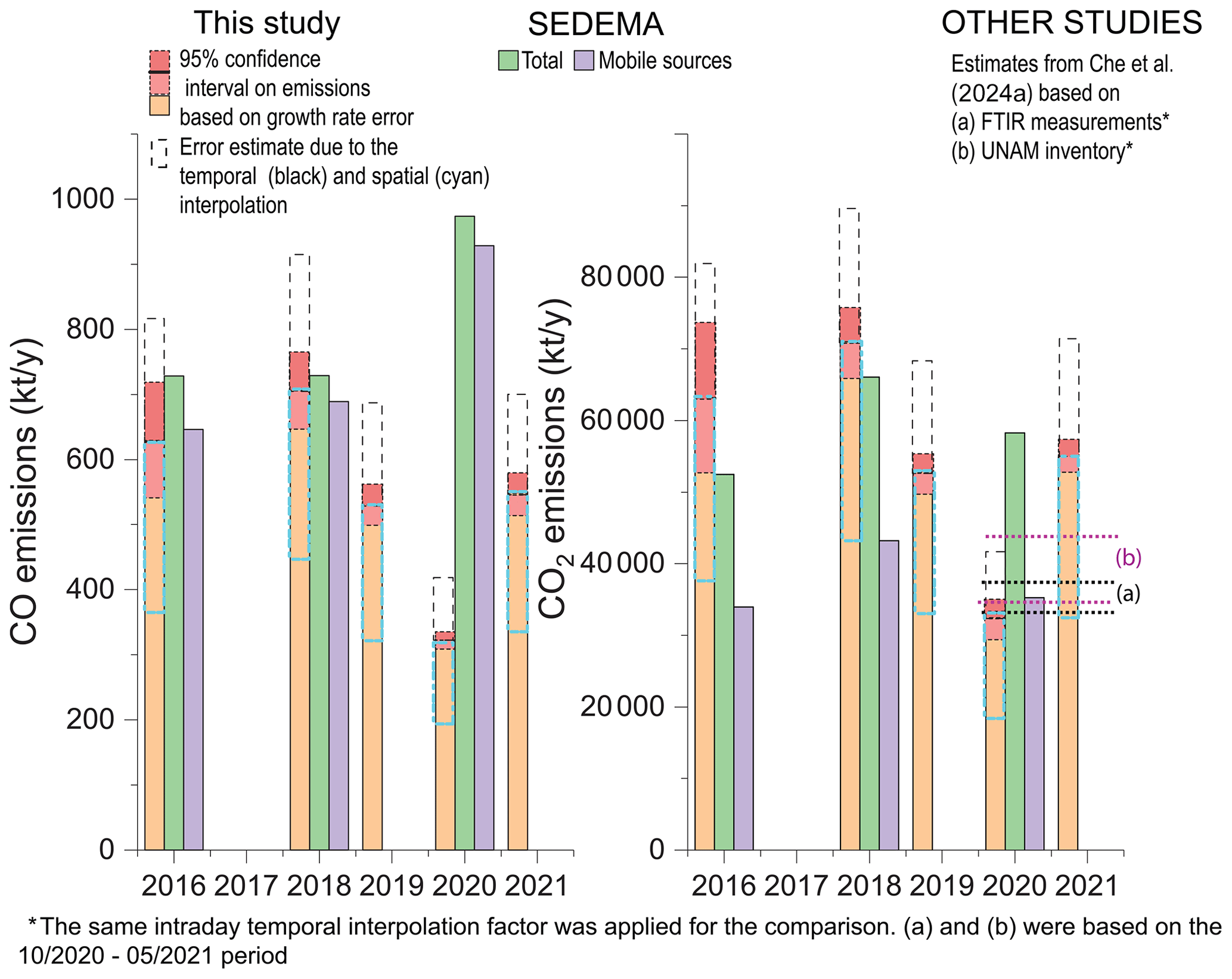
Figure 11 Comparison of CO and CO₂ emission estimates from UNA FTIR diurnal growth rates and from SEDEMA inventories. For CO₂ (right), the estimates from Che et al. (2024a) are also reported, although the values are based on the October 2020 to May 2021 period, after applying the same intraday temporal factor as used for our study to convert gigagrams per hour to kilotons per year.

CO₂ emission could not be directly estimated using the same method, given its complex diurnal pattern, which is a cumulative result of both natural and anthropogenic contributions and has likely been influenced by additional factors, related to instrumental and retrieval effects (i.e. air mass dependence error, with a sub-percentage contribution for CO₂, and non-ideal column sensitivity of the retrieval, which represents a near 25 % overestimation for the CO₂ anomaly and a 5 % underestimation for the CO anomaly in the PBL). Instead, we based our CO₂ estimates on the measured XCO / XCO₂ ratio. The average XCO / XCO₂ molecular ratio (0.0164 ± 0.0003) determined from the UNA and VAL total column measurement (Fig. 9) was converted to a mass ratio (by multiplying it by the molecular weight ratio) and found to be 0.0100 ± 0.0002. Considering this ratio, we estimated the CO₂ annual emission as 71 ± 6 (42 ± 4) Tg yr⁻¹ for 2018. Our estimates of CO and CO₂ emissions by year and their average over the whole time series, applying the same method, are presented in Fig. 11 and Table S3, along with the SEDEMA inventories for the MCMA. We obtained 2016–2021 average CO and CO₂ emission values of 0.55 ± 0.02 (0.32 ± 0.01) and 46 ± 2 (32 ± 1) Tg yr⁻¹, respectively, when excluding the lockdown period (Table S3). Here, the given uncertainties are solely those stemming from the propagation of errors in growth rate estimates. Uncertainties in the absolute values are much higher when considering spatial and temporal extrapolations errors, but they do not influence the interpretation of relative values.

5 Discussion

5.1 Long-term variability

In this contribution, we characterized the seasonal and interannual variability and trends in the CO and CO₂ total column and surface concentrations from two urban stations and one background station. The average 2013–2019 total column growth rate obtained at ALTZ (∼ 2.5 ppm yr⁻¹) and its interannual variability are in accordance with that typical of Northern Hemisphere measurements from TCCON stations (hereafter referred to as NH-TCCON) (Sussmann and Rettinger, 2020; AGR of 2.4 ppm yr⁻¹ for the 2012–2019 period).

Both the NH-TCCON and ALTZ stations captured an important increase in the AGR in 2016 (+1.1 ppm yr⁻¹ for the TCCON stations and +2.1 ppm yr⁻¹ for the ALTZ station with respect to 2015), coinciding with the most intense ENSO (El Niño–Southern Oscillation) event since the 1950s. The impact of El Niño events on the carbon cycle is not yet fully understood, although they are consistently accompanied by a global increase in XCO₂ due to increasing drought in many regions and a decrease in global land carbon uptake. In 2016, an increase of +1.3 ppm yr⁻¹ was observed in the Mauna Loa in situ AGR with respect to 2015 (Betts et al., 2018); the contribution of the El Niño event was estimated to be about 25 %, with the rest ascribed to an increase in the anthropogenic emissions. In Mexico, El Niño events are generally associated with a decrease in precipitation, with deficits that can reach up to 250 mm in the southwestern area of the country, causing drought and a higher occurrence of wild and forest fires (Bravo Cabrera et al., 2018; González del Castillo et al., 2022). Our observations from the ALTZ measurements highlight a much higher XCO₂ increase (+2.1 ppm yr⁻¹) during 2016 with respect to 2015 than that observed at the NH-TCCON stations. During this period, a small increase in the XCO MAGR ($\sim +\mathrm{0.02}$ ppm) is also observed at both the ALTZ and UNA stations, maintaining the highest values of the whole time series over more than 4 months. Assuming that the CO MAGR variability captured at the ALTZ station during 2016 rather reflects a change in the MCMA's global emissions, we attempt to delineate the global and local contributions in the 2016 XCO₂ ALTZ AGR increase. Adopting a molecular $\mathrm{CO}/{\mathrm{CO}}_{\mathrm{2}}$ ratio of ∼ 0.016, a hypothetical increase in the XCO₂ MAGR over the September 2015–September 2016 period due to the local emissions would be around 1.2 ppm yr⁻¹, or about 60 % of the observed increasing rate during this period (2.1 ppm yr⁻¹). This gross estimate suggests that the El Niño regional effect only contributed to about 25 % (0.9 ppm) of the observed AGR increase, which is close to the estimate from the NH-TCCON stations ($\sim +\mathrm{1.1}$ ppm) and from in situ data.

On the other hand, our long-term FTIR and surface time series allow for the examination of the effect of the COVID-19 lockdown on the tropospheric CO₂ and CO concentration above the MCMA at local and regional scales. The reduction in the surface CO and CO₂ AGR at UNA (CO₂ AGR decreased to a value close to zero, while CO AGR was ∼ −0.1 ppm yr⁻¹) with respect to the other years (Fig. 3) and the strong diminution of their amplitude in the mean diurnal cycles clearly reflect a significant decrease in local emissions near the UNA station, likely due to a drastic reduction in urban traffic (the average annual congestion level decreased from 52 % in 2019 to 36 % in 2020 in Mexico City, based on available TomTom estimates: https://www.tomtom.com/traffic-index/mexico-city-traffic/, last access: 1 March 2024).

The FTIR total column XCO₂ and XCO time series at UNA did not capture such a drastic change: only a small short-term decrease in the MAGR that was lower than the standard deviation of the whole time series was observed between April and October 2020. These results are in accordance with previous studies in other parts of the world. Although a reduction of 8.8 % of the global CO₂ emissions was observed during the first 5 months of 2020 (Liu et al., 2020; Jones et al., 2021), and an annual reduction from 4 % to 7 % was found (Le Quéré et al., 2020), the atmospheric total column XCO₂ showed a less clear effect (Sussmann and Rettinger, 2020).

5.2 The $\mathrm{CO}/{\mathrm{CO}}_{\mathrm{2}}$ ratio and MCMA emission estimates

In this study, we robustly determined the $\mathrm{CO}/{\mathrm{CO}}_{\mathrm{2}}$ ratio characterizing the combustion efficiency of the city (0.016 ± 0.01) from both surface and total column measurements at two urban stations. We found the same ratio for the UNA and VAL stations, and this ratio is very consistent with that found using the (UNA − VAL) gradients and the surface measurements. This ratio is also consistent with that reported by MacDonald et al. (2023), calculated from TROPOMI and OCO-2/OCO-3 measurements (0.019), and slightly higher than that obtained from the EDGAR, FFDAS and ODIAC inventories (ratio ∼ 0.012) reported in the same study.

Our estimate of CO emissions from the UNA measurements is based on a simplified approach, limited to days with low ventilation and time intervals corresponding to the late-morning hours. It assumes a homogeneous area within the footprint and averages selected days without discrimination. Given that spatiotemporal extrapolation introduces large uncertainties, only the relative and interannual behaviour of the emissions can be discussed here; however, the approach demonstrates how closely the column growth rate can be related to the emission flux if meteorological conditions allow for advection to be neglected. Our estimated range of CO emissions is consistent with the SEDEMA inventories, at least for the years 2016 (factor 0.98) and 2018 (factor 1.04), if we consider that they are dominated by the mobile sources. However, this is not the case for 2020, during which our estimate is much lower than that of SEDEMA (by a factor of 0.3). During the lockdown period, we estimated a decrease of about 55 % compared with 2018, whereas 2020 is the year with maximum CO emissions (increase of 35 % compared with 2018 considering the mobile sources) in the SEDEMA report. Both of these estimates contrast with Kutralam-Muniasamy et al. (2021), who reported an increase of 1.1 % during the lockdown using the RAMA surface data. The large difference observed between these different studies could be due to (i) the different methods used for extrapolating the emissions in space and time, (ii) the higher uncertainties in the FTIR-based estimates due to an important reduction in the selected measurement days and (iii) an overestimation in the SEDEMA inventory due to a lack of data during the lockdown period. Our estimate is based on the extrapolation of data from only one station (UNA), for which the dominant source is mainly UNAM traffic activity. During the lockdown, UNAM was closed, and a significant reduction in the local traffic was recorded; however, this traffic reduction was likely not representative of the whole of the MCMA. Nevertheless, the decrease in the MAGR at both the VAL and UNA stations does not support the increase in the CO emissions estimated by the SEDEMA inventory. Interestingly, it was not possible to apply the same method to calculate CO emissions at VAL because the average growth rate was close to zero (Fig. 6). This behaviour at VAL is likely due to the fast dispersion of the pollutants at this site, weakening the link between the diurnal pattern and the emissions.

Regarding CO₂, our estimates also agree with the SEDEMA inventory, especially if we consider the total emissions instead of mobile sources (factor of 1.2 and 1.1) for the years 2016 and 2018. For 2020, we estimated a decrease of 55 %, whereas the SEDEMA inventory indicates a decrease of about 10 %. The $\mathrm{CO}/{\mathrm{CO}}_{\mathrm{2}}$ ratios calculated from the SEDEMA data for total emissions are similar to ours (0.014 and 0.011 in 2016 and 2018, respectively), suggesting that our average $\mathrm{CO}/{\mathrm{CO}}_{\mathrm{2}}$ ratio is actually representative of the global mixing of the different sources in the MCMA, not only of those dominated by the road traffic. Interestingly, according to the SEDEMA inventory, road traffic, the main anthropogenic CO source, is identified by ratios (0.019 and 0.016 in 2016 and 2018, respectively) that are only slightly higher than our global average, whereas the industrial and domestic burning sectors, which represent the second main CO₂ anthropogenic emissions source, produce a ratio that is 1 order of magnitude lower. In any case, our measurements are representative of the main source of the CO and CO₂ anthropogenic emissions. Indeed, if we consider the 2018 SEDEMA ratio for mobile sources (0.016), we find CO₂ emissions of the order of 43 100 kt yr⁻¹ for this year, which is within ∼ 5 % of the SEDEMA estimates.

Our results were also compared with the estimates reported in Che et al. (2023, 2024a), based on an intensive FTIR measurement campaign performed during the October 2020 to May 2021 period and using the Column-Stochastic Time-Inverted Lagrangian Transport (X-STILT) model and a Bayesian inversion (Fig. 11). Considering the same measurement period, our method leads to CO₂ emission estimates ranging between 29 000 and 49 800 kt yr⁻¹ using the respective inner and outer effective areas; this is consistent with the estimates obtained in Che et al. (2024a), which ranged between 32 700 and 37 200 kt yr⁻¹ when applying the same intraday temporal extrapolation factor. Although the method that we used for estimating the MCMA emissions is coarse and contains large uncertainties, mainly due to the spatiotemporal extrapolation, it shows the ability to use one station to capture the variability in the anthropogenic emissions of the MCMA and provide year-by-year follow-up emission information without using complex dispersion models.

6 Summary and conclusion

We have analysed the variability in the total column XCO and XCO₂ above the MCMA from two urban stations and one background station. The long-term XCO₂ data at the ALTZ station show an average annual growth rate of ∼ 2.4 ppm yr⁻¹, similar to what has been reported from TCCON stations in the Northern Hemisphere, and captured the perturbation driven by the 2015–2016 El Niño event. The urban stations show a similar growth rate (∼ 2.3 ppm yr⁻¹), and, in contrast to results from ALTZ, a slight decrease in XCO₂ and XCO during the COVID-19 lockdown period could be observed. The CO₂ and CO concentrations within the mixed layer, estimated from the FTIR total column measurements and ceilometer data, were found to be consistent with the surface measurements. These findings confirm that the concentrations near the surface are mainly controlled by the emissions and the daily behaviour of the mixed layer in the MCMA. Our long-term total column and surface time series from both urban stations allowed us to determine, with great confidence, an average $\mathrm{CO}/{\mathrm{CO}}_{\mathrm{2}}$ ratio indicative of the Mexico City combustion efficiency. The $\mathrm{CO}/{\mathrm{CO}}_{\mathrm{2}}$ ratio over our long-term measurement period seems to be fairly constant and equals ∼ 0.016 (mass ratio of 0.010). This value is consistent with other studies, such as those using satellite measurements (OCO-2/OCO-3 and TROPOMI) and the bottom-up inventories reported by MacDonald et al. (2023). Finally, we estimated the CO emissions using the average daily growth rate determined from measurements at UNA station. Although this method likely leads to an underestimate of the emissions due to the non-negligible effects of advection, our results were found to be very consistent with the 2016 and 2018 SEDEMA inventories. The same strategy could not be applied at the VAL station, likely owing to the dominant southward advection of air masses due to the complex topography in this part of the MCMA. In contrast, UNA station is located on flat ground and downwind of the main anthropogenic source in the MCMA; this likely allows for the establishment of a direct relationship between the columnar measurements and the MCMA CO and CO₂ emissions. Moreover, we estimated the CO₂ emissions using the CO growth rate and the $\mathrm{CO}/{\mathrm{CO}}_{\mathrm{2}}$ ratio. The finding that our CO₂ emission estimates are within 20 % of those of SEDEMA for total emissions shows that our ratio not only reflects the traffic sources; it is also affected by other sources such as industrial activities and domestic burning. UNA station, with its advantageous orography, is therefore a good site to capture well-mixed emissions from the city, and it serves as a site to follow the interannual variability and trends in the emissions in this urban environment. Finally, this study showed the feasibility of monitoring the long-term evolution of anthropogenic CO₂ and CO emissions in Mexico City by deploying only a few EM27/SUN instruments. The methodology employed here for monitoring the long-term temporal variability in the CO emission fluxes is likely to be adapted to other urban areas where the topography dampens the ventilation for several hours each day, thereby establishing that the column growth rate is dominated by the emission flux. Although the straightforward model presented here is not intended to replace a complex transport/chemical model for a precise estimate of city emissions, the results obtained demonstrate that it is nevertheless possible to track their temporal evolution with a high degree of reliability.