Present-day methane shortwave absorption mutes surface warming relative to preindustrial conditions

Recent analyses show the importance of methane shortwave absorption, which many climate models lack. In particular, Allen et al. (2023) used idealized climate model simulations to show that methane shortwave absorption mutes up to 30 % of the surface warming and 60 % of the precipitation increase associated with its longwave radiative effects. Here, we explicitly quantify the radiative and climate impacts due to shortwave absorption of the present-day methane perturbation. Our results corroborate the hypothesis that present-day methane shortwave absorption mutes the warming effects of longwave absorption. For example, the global mean cooling in response to the present-day methane shortwave absorption is $-\mathrm{0.10}\pm \mathrm{0.07}$ K, which offsets 28 % (7 %–55 %) of the surface warming associated with present-day methane longwave radiative effects. The precipitation increase associated with the longwave radiative effects of the present-day methane perturbation (0.012±0.006 mm d⁻¹) is also muted by shortwave absorption but not significantly so ($-\mathrm{0.008}\pm \mathrm{0.009}$ mm d⁻¹). The unique responses to methane shortwave absorption are related to its negative top-of-the-atmosphere effective radiative forcing but positive atmospheric heating and in part to methane's distinctive vertical atmospheric solar heating profile. We also find that the present-day methane shortwave radiative effects, relative to its longwave radiative effects, are about 5 times larger than those under idealized carbon dioxide perturbations. Additional analyses show consistent but non-significant differences between the longwave versus shortwave radiative effects for both methane and carbon dioxide, including a stronger (negative) climate feedback when shortwave radiative effects are included (particularly for methane). We conclude by reiterating that methane remains a potent greenhouse gas.

1 Introduction

Several recent studies (Li et al., 2010; Etminan et al., 2016; Collins et al., 2018; Byrom and Shine, 2022) have shown the significance of methane (CH₄) shortwave (SW) absorption – which is lacking in many climate models (Forster et al., 2021) – at near-infrared (NIR) wavelengths. Etminan et al. (2016) first showed methane SW absorption increases its stratospherically adjusted radiative forcing (SARF) by up to ∼ 15 % compared to its longwave (LW) SARF. Smith et al. (2018) subsequently inferred negative rapid adjustments (i.e., surface-temperature-independent responses; see Sect. 2) due to CH₄ SW absorption, using 4 of 10 models from the Precipitation Driver Response Model Intercomparison Project (PDRMIP; Myhre et al., 2017) that included an explicit representation of methane SW absorption. Byrom and Shine (2022) showed that CH₄ SW forcing depends on several factors, including the spectral variation in surface albedo; the vertical profile of methane; and absorption of solar radiation at longer wavelengths, specifically methane's 7.6 µm band. They estimated a smaller impact of CH₄ SW absorption, with a 7 % increase in SARF, in part due to the inclusion of the 7.6 µm band that mainly impacts stratospheric solar absorption.

The recent analysis of Allen et al. (2023) (hereafter referred to as A23) used Community Earth System Model version 2 (CESM2; Danabasoglu et al., 2020) simulations to isolate the effects of CH₄ SW absorption and showed that it muted the surface warming and wetting due to methane's LW radiative effects. Muting of surface warming was attributed largely to cloud rapid adjustments, including increased low-level clouds and decreased high-level clouds. These cloud changes in turn were associated with the vertical profile of atmospheric solar heating and with corresponding changes to atmospheric temperature and relative humidity.

We adopt similar terminology as in A23. Throughout this paper, the terms “SW radiative effect/SW absorption” and “LW radiative effect” refer to the radiative effects of methane (and eventually carbon dioxide) on the climate system as isolated by a suite of simulations (to be discussed below). This terminology is used interchangeably with the abbreviations “CH_4SW” and “CH_4LW”, respectively.

A23 focused on three idealized methane perturbations, including 2x, 5x and 10x preindustrial methane concentrations. Relatively large perturbations were emphasized to maximize the signal-to-noise ratio, as well as to robustly identify mechanisms. Despite these relatively large methane perturbations, 5x preindustrial methane concentrations are comparable to projections from the end of the 21st century under the Shared Socioeconomic Pathway 3–7.0 (i.e., 0.75 to 3.4 ppm). Although 5xCH₄ and 10xCH₄ SW radiative effects showed a clear muting of the corresponding LW effects, 2xCH₄ did not. For example, the global mean near-surface air temperature (TAS) response under 5xCH_4SW and 10xCH_4SW yielded significant global cooling at $-\mathrm{0.23}\pm \mathrm{0.07}$ and $-\mathrm{0.39}\pm \mathrm{0.07}$ K. We reiterate that this cooling is due to isolation of methane's shortwave absorption alone; the total (including methane's longwave absorption) temperature response is significant warming at 0.45±0.05 and 0.85±0.05 K, respectively (i.e., longwave absorption effects dominate). The 2xCH_4SW, however, yielded a warming response of 0.06±0.06 K that is not significant at the 90 % confidence level. Similar results apply for the global mean precipitation (P) response, where a significant decrease occurred under 5xCH_4SW and 10xCH_4SW at $-\mathrm{0.021}\pm \mathrm{0.008}$ and $-\mathrm{0.039}\pm \mathrm{0.008}$ mm d⁻¹ (−0.7 % and −1.3 %). For 2xCH_4SW, the response was again not significant at 0.002±0.008 mm d⁻¹ (0.06 %). The lack of significant climate responses in the 2xCH_4SW coupled ocean–atmosphere simulation is consistent with its relatively weak forcing compared to the larger methane perturbations and relative to internal climate variability in the coupled ocean–atmosphere system.

Here we conduct analogous simulations to A23 to explicitly calculate the shortwave absorption effects of the present-day methane concentration, i.e., the ∼ 750 to ∼ 1900 ppb increase (∼ 2.5x). Our results support the prior conclusions from A23. We further expand upon our understanding of the climate effects of CH_4SW by conducting an atmospheric energy budget analysis, by evaluating the climate feedback and hydrological sensitivity parameters (and climate sensitivity), and by comparing the effects of methane SW absorption with those from carbon dioxide SW absorption.

2 Materials and methods

An array of targeted methane-only and carbon-dioxide-only equilibrium time slice (i.e., cyclic repetition of the imposed perturbation) climate simulations are conducted with CESM2 (Danabasoglu et al., 2020), which includes the most recent model components such as the Community Atmosphere Model version 6 (CAM6). CAM6's radiation parameterization, the Rapid Radiative Transfer Model for general circulation models (RRTMG; Iacono et al., 2008), includes a representation of CH₄ SW absorption in three near-infrared bands including 1.6–1.9 µm, 2.15–2.50 µm and 3.10–3.85 µm. Methane shortwave absorption at 7.6 µm (the mid-infrared or mid-IR), however, is not represented. Furthermore, although CESM2 includes a representation of CH₄ SW absorption, RRTMG underestimates CH₄ (and CO₂) SW instantaneous radiative forcing (IRF) by 25 %–45 % (Hogan and Matricardi, 2020).

Our focus here is a set of 2.5x preindustrial atmospheric CH₄ concentration simulations, to complement the three methane perturbations (2x, 5x and 10x preindustrial atmospheric CH₄ concentrations) performed by A23. We perform both fixed climatological sea surface temperature (fSST) simulations and fully coupled ocean–atmosphere simulations (Table 1), and we conduct two sets of identical experiments: one that includes CH₄ LW + SW radiative effects ($\mathrm{2.5}{\mathrm{xCH}}_{\mathrm{4}}^{\mathrm{EXP}}$) and one that lacks CH₄ SW radiative effects ($\mathrm{2.5}{\mathrm{xCH}}_{\mathrm{4}\mathrm{NOSW}}^{\mathrm{EXP}}$). CH₄ SW absorption in the three NIR bands in RRTMG is turned off in the simulations that lack methane SW absorption. These are compared to a default preindustrial control experiment (PIC^EXP), which includes CH₄ (as well as other radiative species such as CO₂) LW + SW radiative effects, as well as to a preindustrial control experiment with CH₄ SW radiative effects turned off (i.e., LW effects only, denoted as ${\mathrm{PIC}}_{\mathrm{NOCH}\mathrm{4}\mathrm{SW}}^{\mathrm{EXP}}$). To clarify, SW changes can still be present in $\mathrm{2.5}{\mathrm{xCH}}_{\mathrm{4}\mathrm{NOSW}}^{\mathrm{EXP}}$ but only as a rapid adjustment (or a temperature-induced response) associated with the direct LW absorption of methane. For example, direct LW absorption of methane can drive changes in water vapor and clouds, which in turn could impact SW radiation.

Table 1 Description of CESM2/CAM6 methane and carbon dioxide experiments. Fixed climatological sea surface temperature simulations and coupled ocean–atmosphere simulations are both performed for each experiment. The 2.5x preindustrial level atmospheric methane concentrations represent the present-day methane perturbation that corresponds to a ∼ 750 to ∼ 1900 ppb increase (i.e., ∼ 150 %). Analogous experiments are conducted for 2xCO₂ and 4xCO₂.

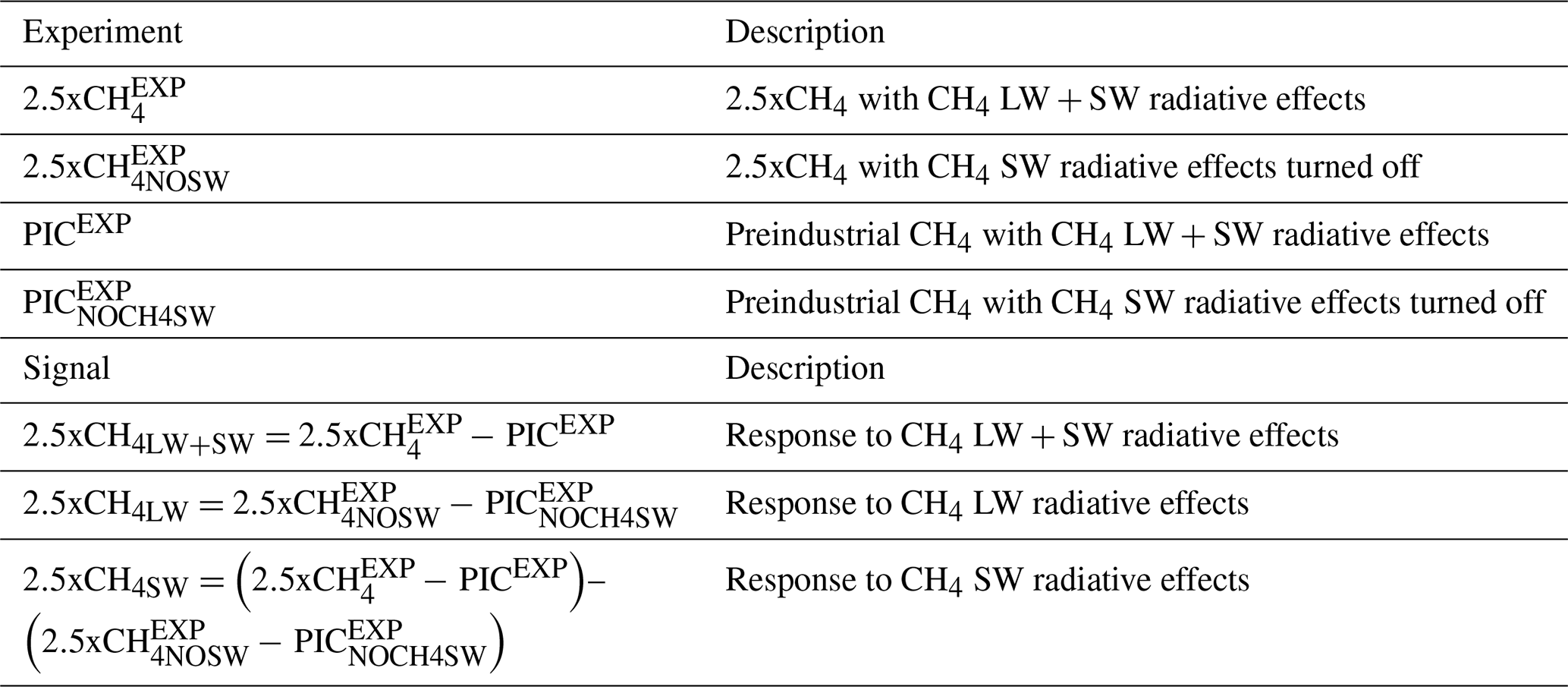
This suite of CH₄ simulations allows quantification of the CH₄ LW + SW, LW and SW radiative effects, denoted as 2.5xCH_4LW+SW, 2.5xCH_4LW and 2.5xCH_4SW. The 2.5xCH_4LW+SW signal is obtained by subtracting the default 2.5xCH₄ perturbation from the default control (2.5xCH${}_{\mathrm{4}}^{\mathrm{EXP}}-{\mathrm{PIC}}^{\mathrm{EXP}}$). The 2.5xCH_4LW signal is obtained by subtracting the 2.5xCH₄ perturbation without CH₄ SW absorption from the corresponding control simulation without CH₄ SW absorption ($\mathrm{2.5}{\mathrm{xCH}}_{\mathrm{4}\mathrm{NOSW}}^{\mathrm{EXP}}-{\mathrm{PIC}}_{\mathrm{NOCH}\mathrm{4}\mathrm{SW}}^{\mathrm{EXP}}$). The 2.5xCH_4SW signal is obtained by taking the double difference, i.e., $\left(\mathrm{2.5}{\mathrm{xCH}}_{\mathrm{4}}^{\mathrm{EXP}}-{\mathrm{PIC}}^{\mathrm{EXP}}\right)-(\mathrm{2.5}{\mathrm{xCH}}_{\mathrm{4}\mathrm{NOSW}}^{\mathrm{EXP}}-{\mathrm{PIC}}_{\mathrm{NOCH}\mathrm{4}\mathrm{SW}}^{\mathrm{EXP}}$). The 2.5xCH_4SW signal therefore represents CH₄ SW absorption and also the impacts of this SW absorption on CH₄ LW rapid adjustments (and surface temperature responses). We also calculate the corresponding instantaneous radiative forcing (IRF), which is defined as the initial perturbation to the radiation balance, using the Parallel Offline Radiative Transfer (PORT) model (Conley et al., 2013). PORT isolates the RRTMG radiative transfer computation from the CESM2-CAM6 model configuration.

Fixed SST experiments are used to estimate the “fast” climate responses and the effective radiative forcing (ERF). ERF is defined as the top-of-the-atmosphere (TOA) net radiative flux difference between the experiment and control simulation, with climatological fixed SSTs and sea ice distributions without any adjustments for changes in the surface temperature over land (Forster et al., 2016). ERF can be decomposed into the sum of the IRF and rapid adjustments (ADJs). Rapid adjustments represent the change in state in response to the initial perturbation (i.e., IRF) excluding any responses related to changes in sea surface temperatures. Rapid adjustments, which, for example, include clouds and water vapor, are estimated using the radiative kernel method (Soden et al., 2008; Smith et al., 2018, 2020) applied to the climatological fixed SST simulations. A radiative kernel is basically the partial derivative of the radiative flux with respect to a variable (e.g., moisture) that changes with temperature. It therefore represents the radiative impacts from small perturbations in a state. To calculate the rapid adjustments, the radiative kernel is multiplied by the change in the climate variable under consideration (from the fSST simulations). The Python-based radiative kernel toolkit of Soden et al. (2008), along with the Geophysical Fluid Dynamics Laboratory (GDFL) radiative kernel, are used here. The method for calculating cloud rapid adjustments with radiative kernels is a bit more involved. Here, we use the kernel difference method (Smith et al., 2018), which employs a cloud-masking correction applied to the cloud radiative forcing diagnostics. The cloud-masking correction is based on the kernel-derived non-cloud adjustments and IRF. A23 showed that this methodology performed well, including a small residual term (i.e., ERF−IRF−ΣADJs$<\sim \mathrm{5}$ % of ERF). Furthermore, similar results were obtained with an alternative radiative kernel based on CloudSat/CALIPSO (Kramer et al., 2019).

The total climate response, which includes the IRF, ADJs and the surface temperature responses, is quantified using the coupled ocean–atmosphere experiments. Specifically, the radiative effects associated with the total climate response are estimated using the same radiative kernel decomposition as above but applied to the coupled ocean–atmosphere simulation. The surface temperature responses (i.e., the “slow” response) are estimated as the difference between the coupled ocean–atmosphere simulations and the climatologically fixed SST experiments. Similarly, the radiative effects associated with the slow response are calculated as the difference between the kernel-derived radiative effects of the total and fast responses.

To reiterate, our framework is to decompose the total response (directly estimated from coupled simulations) into a fast (surface-temperature-independent) response and a slow (surface-temperature-dependent) response:

$$\begin{array}{}\text{(1)}& \mathrm{Total}\mathrm{response}=\mathrm{fast}\mathrm{response}+\mathrm{slow}\mathrm{response}.\end{array}$$

The fast response is directly estimated from the fSST simulations and includes the rapid adjustments. The slow response is estimated from the difference in the total and fast responses (i.e., the coupled simulation minus fSST simulation). This is consistent with the Intergovernmental Panel on Climate Change (IPCC) framework, which uses the concepts of an adjustment to an imposed forcing (i.e., independent of surface temperature) and a radiative response to a global mean temperature change. It is also analogous to the methodology employed in several other papers, including many PDRMIP papers (e.g., Samset et al., 2016; Myhre et al., 2017).

Our simulations are performed at a 1.9° × 2.5° latitude–longitude resolution with 32 atmospheric levels. Coupled ocean–atmosphere experiments are initialized from a spun-up preindustrial control simulation and subsequently integrated for 90 years. Total climate responses are estimated using the last 40 years of these coupled ocean–atmosphere experiments. As climatologically fixed SST simulations equilibrate more quickly, these are run for 32 years. The ERF and rapid adjustments are estimated from the last 30 years of these fSST experiments.

Our integration lengths are consistent with other related idealized time-slice studies including, for example, a 100-year integration (and analysis of the last 50 years) of coupled simulations under PDRMIP (e.g., Samset et al., 2016; Myhre et al., 2017). A similar statement applies for the integration length of our fSST runs, e.g., the Radiative Forcing Model Intercomparison Project (RFMIP; Pincus et al., 2016) specifies 30-year fSST simulations.

We note that even with a 90-year coupled ocean simulation, the model has not yet reached equilibrium. Given computational resource limitations, there is always a tradeoff between the number of simulations performed and length of each simulation.

A two-tailed pooled t test is used to assess the statistical significance of a climate response based on the annual mean difference between the experiment and control. We evaluate a null hypothesis of zero difference with $n_{\mathrm{1}}+n_{\mathrm{2}}-\mathrm{2}$ degrees of freedom. Here, n₁ and n₂ are the number of years in the experiment and control simulations (e.g., 40 years for the coupled ocean–atmosphere runs). The pooled variance $S_{\mathrm{p}}^{\mathrm{2}}=\frac{\left(n\mathrm{1}-\mathrm{1}\right)S_{\mathrm{1}}^{\mathrm{2}}+(n\mathrm{2}-\mathrm{1})S_{\mathrm{2}}^{\mathrm{2}}}{n\mathrm{1}+n\mathrm{2}-\mathrm{2}}$ is used, where $S_{\mathrm{1}}^{\mathrm{2}}$ and $S_{\mathrm{2}}^{\mathrm{2}}$ are the sample variances. Quoted uncertainty estimates are based on the 90 % confidence interval using the pooled variance according to 1.65×S_p.

3 Results

3.1 2.5xCH₄ radiative flux components and rapid adjustments

Figure 1a shows the 2.5xCH₄ TOA ERF, IRF and ADJ, as well as the radiative kernel decomposition of ADJ (Fig. 1b). The 2.5xCH₄ TOA LW IRF is 0.46±0.05 W m⁻² and the corresponding TOA SW IRF is 0.06±0.07 W m⁻² (not significant at the 90 % confidence level).

The 2.5xCH₄ instantaneous shortwave heating rate (QRS) profile (Fig. 2a) exhibits positive values for atmospheric pressure levels less than ∼ 700 hPa and negative values for pressure levels greater than ∼ 700 hPa. As discussed in A23, increasing the atmospheric methane concentration does not increase lower-tropospheric SW heating because the three near-infrared bands are already highly saturated here (e.g., due to water vapor absorption). Furthermore, the methane-induced QRS increase aloft decreases the available solar radiation in the three near-IR methane absorption bands (1.6–1.9, 2.15–2.50 and 3.10–3.85 µm) that can be absorbed by other gases (e.g., water vapor) in the lower troposphere. This results in the decrease in SW heating rate in the lower troposphere (Fig. 2a). Both of these features exist under 2.5xCH_4SW and are consistent with the other methane perturbations, with the larger perturbations (e.g., 5xCH_4SW) yielding larger QRS increases aloft and larger QRS decreases in the lower troposphere.

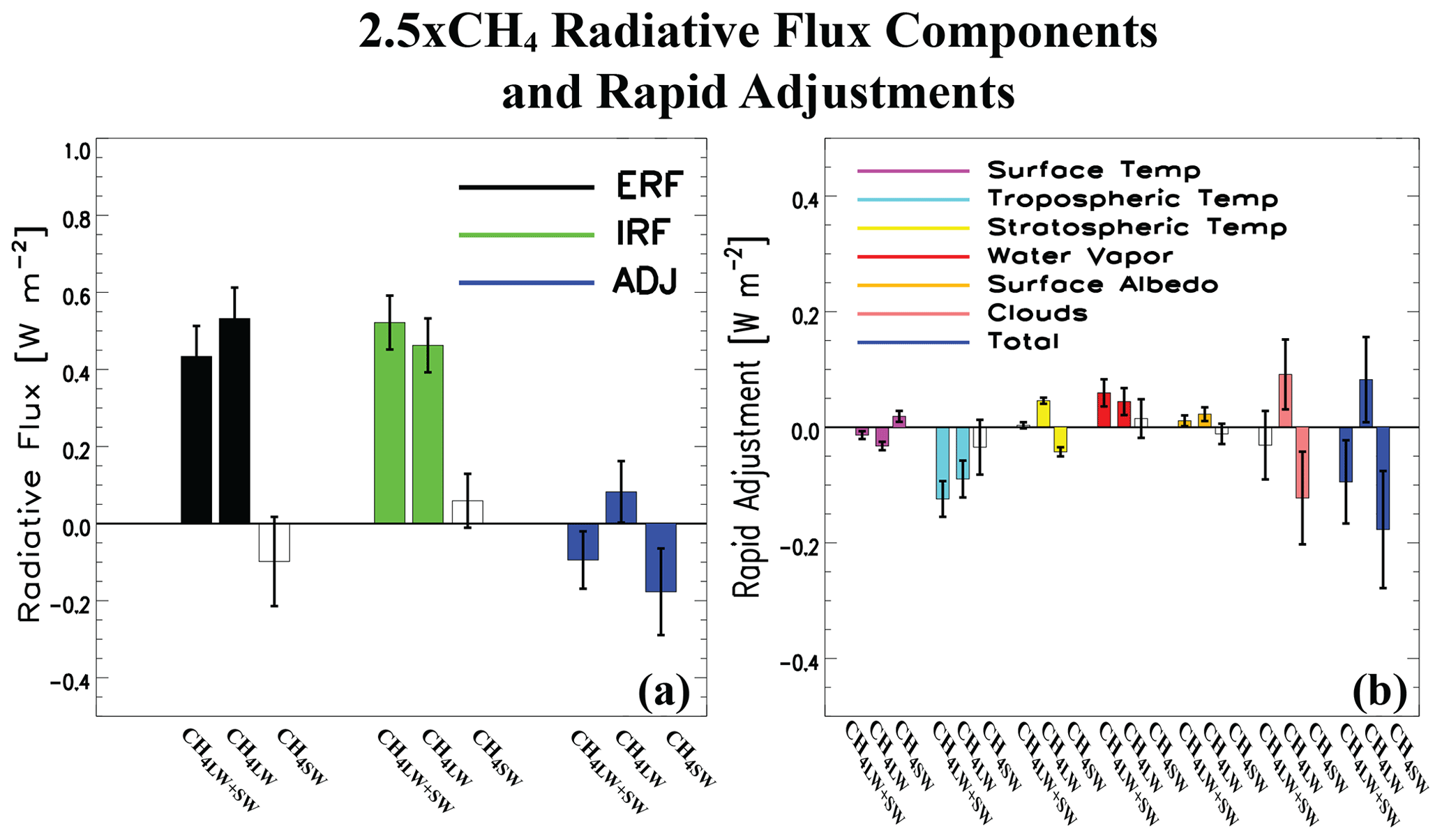
Figure 1 Top-of-the-atmosphere radiative flux components and rapid adjustments for 2.5xCH₄. Global annual mean top-of-the-atmosphere (TOA) (a) effective radiative forcing (ERF; black), instantaneous radiative forcing (IRF; green) and rapid adjustment (ADJ; blue) and (b) decomposition of the rapid adjustment into its components including surface temperature (purple), tropospheric temperature (cyan), stratospheric temperature (yellow), water vapor (red), surface albedo (orange), cloud (pink) and total rapid adjustment (blue) for 2.5xCH₄. Responses are decomposed into methane longwave and shortwave radiative effects (CH_4LW+SW), methane longwave radiative effects (CH_4LW), and methane shortwave radiative effects (CH_4SW). ERF and rapid adjustments are based on 30-year fixed climatological sea surface temperature simulations. Uncertainty is quantified using the 90 % confidence interval; unfilled bars denote responses that are not significant at the 90 % confidence level (units: W m⁻²).

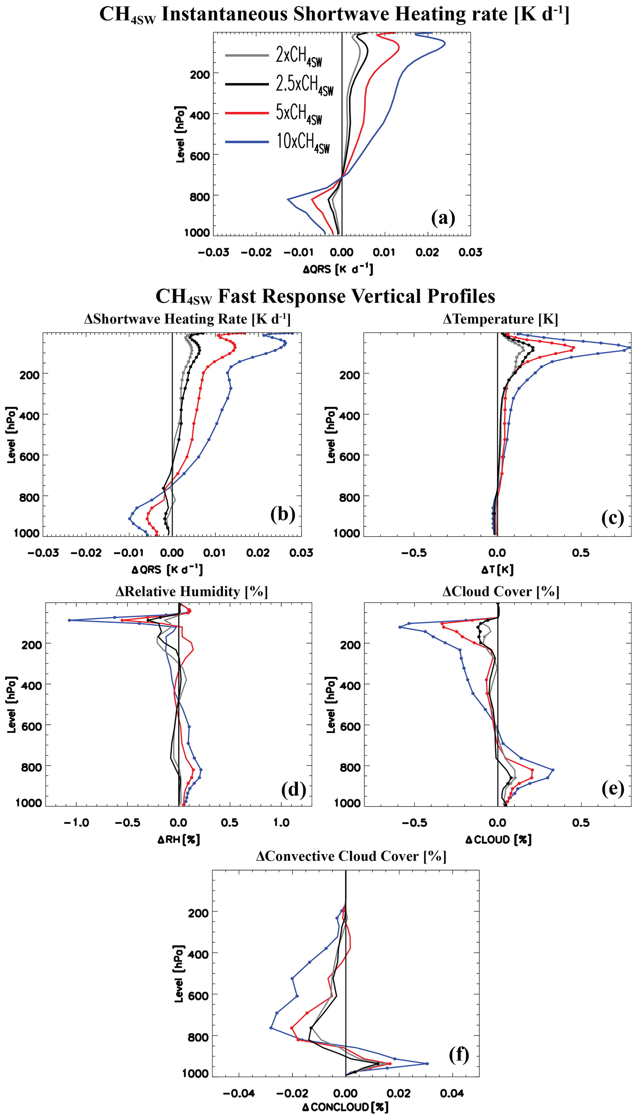
Figure 2 Global mean annual mean vertical-response profiles for four CH_4SW perturbations. Instantaneous (a) shortwave heating rate (QRS; units are K d⁻¹) and (b–f) fast responses of (b) QRS (units are K d⁻¹), (c) air temperature (T; units are K), (d) relative humidity (RH; units are %), (e) cloud cover (CLOUD; units are %) and (f) convective cloud cover (CONCLOUD; units are %) for 2xCH_4SW (gray), 2.5xCH_4SW (black), 5xCH_4SW (red) and 10xCH_4SW (blue). The 2xCH₄, 5xCH₄ and 10xCH₄ simulations are from A23. A significant response at the 90 % confidence level based on a standard t test is denoted by solid dots in (b–f). Climatologically fixed SST simulations are used to estimate the fast responses. Instantaneous QRS profiles come from the Parallel Offline Radiative Transfer Model (PORT).

As mentioned above, A23 showed that methane SW radiative effects lead to a negative rapid adjustment (largely due to changes in clouds) that acts to cool the climate system. A positive ADJ represents a net energy increase, whereas a negative ADJ represents a net energy decrease. Individual rapid adjustments, as well as the total adjustment, under 2.5xCH₄ are displayed in Fig. 1b. Under 2.5xCH_4SW, the total rapid adjustment is $-\mathrm{0.16}\pm \mathrm{0.10}$ W m⁻², which is largely due to the cloud adjustment at $-\mathrm{0.12}\pm \mathrm{0.08}$ W m⁻². The stratospheric temperature adjustment contributes the remainder at $-\mathrm{0.04}\pm \mathrm{0.01}$ W m⁻². The remaining terms (i.e., surface temperature, tropospheric temperature, surface albedo and water vapor adjustments), most of which are not significant at the 90 % confidence level, have a net zero contribution to the total adjustment (i.e., their sum is zero). Thus, similar to the larger CH₄ perturbations in A23, 2.5xCH_4SW yields a significant negative total rapid adjustment that is largely due to the cloud adjustment.

This negative rapid adjustment promotes a negative ERF under methane SW absorption. We reiterate that the negative ERF is due to isolation of methane shortwave absorption alone; methane's longwave effects still dominate the ERF. This is because the ERF is the sum of ADJs and IRF. For example, under the larger 5xCH_4SW perturbation in A23, the ERF and ADJ were both significant, at $-\mathrm{0.22}\pm \mathrm{0.17}$ W m⁻² and $-\mathrm{0.36}\pm \mathrm{0.13}$, respectively. Under 2.5xCH_4SW, the ERF and ADJ (Fig. 1a) are $-\mathrm{0.10}\pm \mathrm{0.13}$ W m⁻² and $-\mathrm{0.16}\pm \mathrm{0.10}$ W m⁻², respectively, with the latter significant at the 90 % confidence level. As with the larger methane perturbations, 2.5xCH_4SW offsets (although not significantly so) ∼ 20 % of the ERF associated with 2.5xCH_4LW (0.53±0.11 W m⁻²).

The corresponding surface CH_4SW ERFs (not shown) are more negative than those at the TOA, at $-\mathrm{0.18}\pm \mathrm{0.10}$ W m⁻² for 2.5xCH_4SW (significant at the 95 % confidence interval). We note that technically this is not an ERF, but we retain this terminology since it is calculated analogously to ERF, just using the surface as opposed to TOA radiative fluxes. This negative surface ERF is consistent with negative surface CH_4SW IRF values (due to atmospheric solar absorption, which decreases surface solar radiation) and with the vertical redistribution of shortwave heating (Fig. 2a) that drives a negative surface rapid adjustment that is again largely due to the cloud adjustment. The surface 2.5xCH_4SW IRF value is $-\mathrm{0.10}\pm \mathrm{0.05}$ W m⁻², and the corresponding sum of the surface rapid adjustments is $-\mathrm{0.08}\pm \mathrm{0.07}$ W m⁻² (not shown).

3.2 2.5xCH_4SW fast climate response

Figure 2b–f show global mean vertical-response profiles from the fSST simulations for the four methane shortwave absorption perturbations (e.g., 2.5xCH_4SW). The 2.5xCH_4SW yields QRS increases (Fig. 2b) in the upper troposphere/lower stratosphere, as well as QRS decreases in the lower troposphere. This is consistent with the aforementioned instantaneous QRS profile response (Fig. 2a). These changes are associated with temperature (Fig. 2c) and relative humidity (RH; Fig. 2d) changes that favor increases in low-level cloud cover (CLOUD; Fig. 2e) that peak near 800 hPa and favor decreases in high-level cloud cover (e.g., for pressures < 300 hPa). Both of these CLOUD responses act to cool the surface. These cloud changes become larger under the larger methane perturbations. For example, 2.5xCH_4SW yields a decrease in global mean lower-tropospheric (pressures > 800 hPa) temperature of $-\mathrm{0.02}\pm \mathrm{0.02}$ K (not significant at the 90 % confidence level) and an increase in upper-tropospheric (between 100 and 500 hPa) temperature of 0.09±0.04 K (significant at the 95 % confidence level). Similarly, global mean lower-tropospheric RH increases by 0.01±0.06 %, and upper-tropospheric RH decreases by $-\mathrm{0.09}\pm \mathrm{0.10}$ % (however, both changes are not significant at the 90 % confidence level). Global mean lower-tropospheric CLOUD increases by 0.045±0.04 % (low cloud as quantified in CESM2 yields 0.08±0.07 %; Table S1 in the Supplement) and upper-tropospheric CLOUD decreases by $-\mathrm{0.07}\pm \mathrm{0.04}$ %.

Correlations between the 2.5xCH_4SW global mean vertical-response profiles are significant. For example, the correlation between the global mean vertical temperature and QRS response profile from 990 to 100 hPa is 0.93. The corresponding correlation between temperature and RH is −0.89, and the corresponding correlation between RH and CLOUD is 0.80. Thus, an increase in SW heating is associated with warming, whereas a decrease in SW heating is associated with cooling. Warming is associated with a decrease in RH, whereas cooling is associated with an increase in RH. Furthermore, an increase in RH is associated with an increase in CLOUD, whereas a decrease in RH is associated with a decrease in CLOUD. These results help to support the importance of atmospheric SW absorption in driving the CLOUD response through altered temperature and RH. Spatial correlations at specific pressure levels also yield similarly significant but somewhat weaker correlations (Fig. S1 in the Supplement). For example, spatially correlating the global mean annual mean change in CLOUD with the corresponding change in RH yields significant correlations in the lower troposphere ranging from 0.40 to 0.65, as well as in the upper troposphere ranging from 0.71 to 0.81. Similar conclusions are obtained with the larger methane perturbations.

These cloud changes are similar to those that occur in response to absorbing aerosols like black carbon (BC; i.e., the aerosol–cloud semi-direct effect; Amiri-Farahani et al., 2019; Allen et al., 2019). Black carbon solar heating warms and dries (decreased relative humidity) the free troposphere, which promotes less cloud cover in the middle to upper troposphere (Stjern et al., 2017). Warming aloft (and cooling of the lower troposphere under CH_4SW) also suggests enhanced lower-tropospheric stability. As lower-tropospheric stability is a measure of the inversion strength that caps the boundary layer, enhanced lower-tropospheric stability traps more moisture in the marine boundary layer, allowing for enhanced cloud cover (e.g., Wood and Bretherton, 2006). Under 2.5xCH_4SW, global mean lower-tropospheric stability (estimated here as the temperature difference between 600 and 990 hPa) significantly increases (at the 95 % confidence level) by 0.03±0.02 K. Larger increases in lower-tropospheric stability occur under the larger methane perturbation, e.g., 0.06±0.02 K under 10xCH_4SW (and similarly, larger increases in low clouds occur at 0.36±0.10 %; Table S1). This increase in low-cloud cover, most of which occurs over the oceans (Fig. S2a, d, g, j), is consistent with the increase in lower-tropospheric stability. Furthermore, enhanced stability also suggests reduced convective mass flux in the middle to upper troposphere. Although we did not archive convective mass flux, Fig. 2f shows changes in convective cloud cover (CONCLOUD). All methane perturbations show decreased CONCLOUD in the middle to upper troposphere (pressures < 800 hPa). CONCLOUD also increases in the lower troposphere (peaking near 900 hPa). Although these CONCLOUD changes are weaker than those associated with CLOUD, their profiles are very similar, implying that changes in convection also contribute to changes in CLOUD.

3.3 2.5xCH_4SW total climate response

Figure 3a–e show global mean vertical total climate response profiles from the coupled ocean–atmosphere simulations for the four methane shortwave absorption perturbations (e.g., 2.5xCH_4SW). The QRS, RH and CLOUD responses are similar to those from the fSST simulation (Fig. 2), which further highlights the importance of rapid adjustments to the total climate response. For example, similar to the fast response, the total response features increases in low- and mid-level clouds (Fig. 3c; peaking near 800 hPa) and decreases in high-level clouds (for pressures < 300 hPa), both of which act to cool the surface (Fig. 3f).

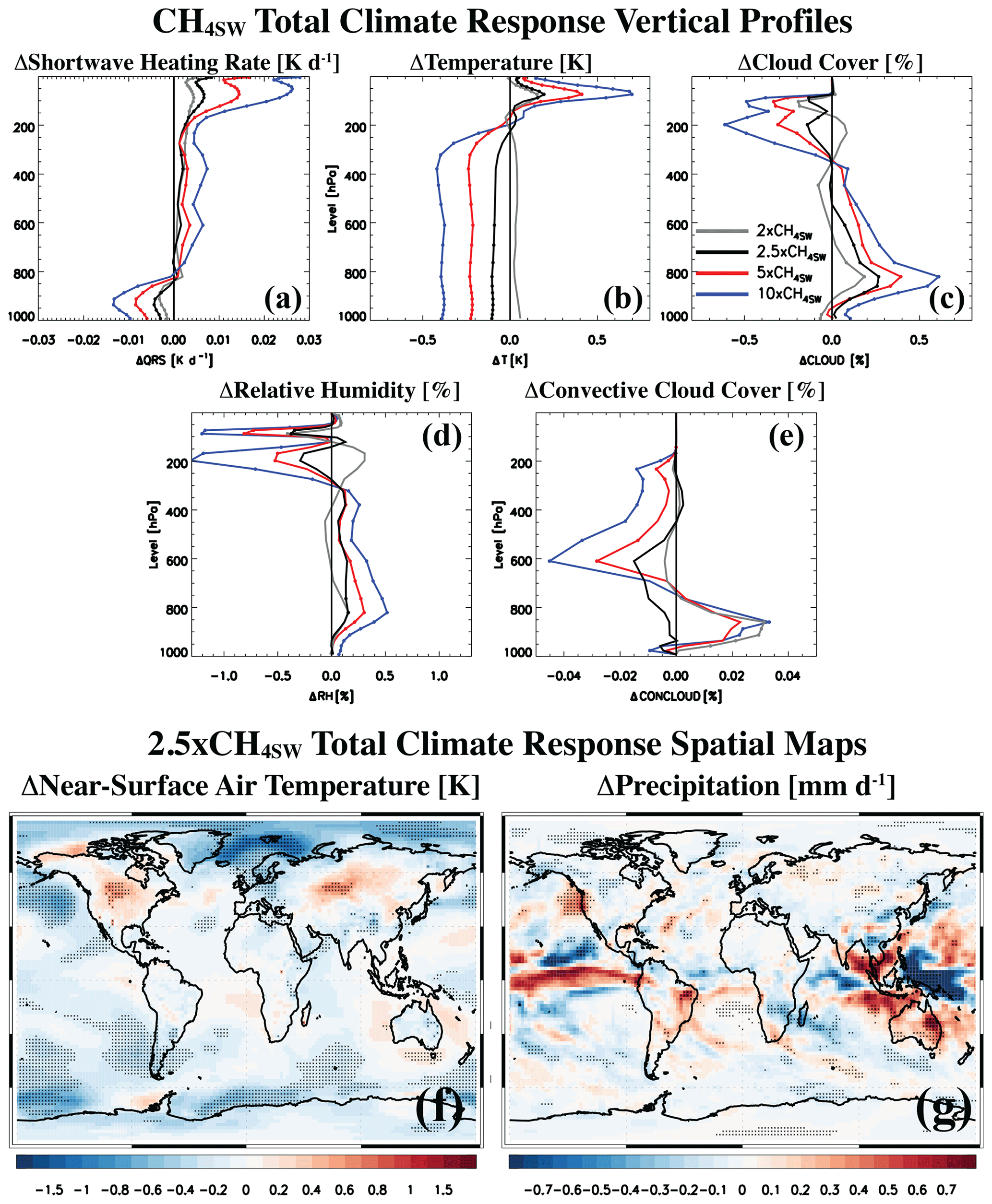
Figure 3 Total climate responses to CH_4SW. Annual mean global mean vertical-response profiles of (a) shortwave heating rate (QRS; units are K d⁻¹), (b) air temperature (T; units are K), (c) cloud cover (CLOUD; units are %), (d) relative humidity (RH; units are %) and (e) convective cloud cover (CONCLOUD; units are %) for 2xCH_4SW (gray), 2.5xCH_4SW (black), 5xCH_4SW (red) and 10xCH_4SW (blue). The 2xCH_4SW, 5xCH_4SW and 10xCH_4SW simulations are from A23. Also included are global maps of the annual mean (f) near-surface air temperature (K) and (g) precipitation (mm d⁻¹) response for 2.5xCH_4SW. A significant response at the 90 % confidence level based on a standard t test is denoted by solid dots. Climate responses are estimated from coupled ocean–atmosphere CESM2 simulations.

Relative to the fast responses discussed above, the total responses are generally similar but larger and more significant in the lower (and middle) troposphere and weaker in the upper troposphere. This is consistent with allowing the surface to respond to the CH_4SW perturbation in the fully coupled ocean–atmosphere experiments, and in particular, consistent with the negative surface CH_4SW ERFs discussed in Sect. 3.1 (i.e., decrease in surface solar radiation). For example, the 2.5xCH_4SW total response features a decrease in global mean lower-tropospheric temperature (Fig. 3b) of $-\mathrm{0.10}\pm \mathrm{0.07}$ K, which is significant at the 95 % confidence level and about 5 times as large as the cooling under the fast response (Fig. 2c). This smaller lower-tropospheric temperature adjustment (i.e., fast response) is consistent with the experimental design (i.e., fixed SSTs). A non-significant decrease in upper-tropospheric temperature of $-\mathrm{0.02}\pm \mathrm{0.11}$ K occurs under the total response, in contrast to the upper-tropospheric warming under the fast response (Fig. 2c). Similarly, global mean lower-tropospheric RH (Fig. 3d) increases by 0.05±0.05 % (significant at the 90 % confidence level) under the 2.5xCH_4SW total response, with a non-significant change in upper-tropospheric RH of $-\mathrm{0.02}\pm \mathrm{0.08}$ %. Global mean lower-tropospheric CLOUD (Fig. 3c) increases by 0.12±0.07 % (significant at the 99 % confidence level), and upper-tropospheric CLOUD decreases by $-\mathrm{0.06}\pm \mathrm{0.03}$ % (significant at the 99 % confidence level). The corresponding changes under the fast response (Fig. 2) are generally similar but smaller in the lower troposphere (i.e., smaller increases in RH and CLOUD) but larger in the upper troposphere (i.e., larger decreases in RH and CLOUD). The total response of CONCLOUD (Fig. 3e) is generally similar to the fast response (Fig. 2f), although the 2.5xCH_4SW total response lacks an increase in the lower troposphere.

Global maps of the TAS and P total climate responses (from coupled ocean–atmosphere simulations) under 2.5xCH_4SW are shown in Fig. 3f, g. The global mean TAS response is $-\mathrm{0.10}\pm \mathrm{0.07}$ K (significant at the 95 % confidence level); the global mean P response is $-\mathrm{0.008}\pm \mathrm{0.009}$ mm d⁻¹ (−0.27 %), which is not significant at the 90 % confidence level. Comparing these 2.5xCH_4SW responses to the corresponding 2.5xCH_4LW responses of 0.36±0.05 K and 0.012±0.006 mm d⁻¹ shows that under 2.5xCH₄, methane shortwave absorption offsets 28 % (7 %–55 %) of the surface warming and 66 % of the precipitation increase associated with its longwave radiative effects. Although the 66 % muting of the precipitation increase is not significant, this percentage is qualitatively consistent with the larger methane perturbations.

As noted in Sect. 3.1, consistent with the larger methane perturbations, the 2.5xCH_4SW ERF at 0.10±0.13 W m⁻² offsets 19 % (although not significant) of the ERF associated with 2.5xCH_4LW. In contrast, 2.5xCH_4SW offsets a larger percentage of the surface warming associated with 2.5xCH_4LW, at 28 %. Based on the global mean TOA energy decomposition equation ΔN =ΔF+αΔTAS (e.g., Forster et al., 2021) where ΔN is the change in the global mean TOA net energy flux (W m⁻²), ΔTAS is the change in global mean near-surface air temperature (K), ΔF is the change in the global mean TOA net energy flux (W m⁻²) when ΔTAS = 0 (i.e., the effective radiative forcing, ERF) and α is the net feedback parameter (W m⁻² K⁻¹). If ΔF is reduced by X %, ΔTAS should also be reduced by X %, assuming a constant α. Table S2 and Fig. S3 show the individual components of the TOA energy decomposition equation, including the estimated climate feedback parameter (details on how these are calculated are included in the corresponding captions). The climate feedback parameter is always larger (in magnitude) under the various SW+LW signals (e.g., 2.5xCH_4LW+SW) compared to the LW-only signal (e.g., 2.5xCH_4LW), which suggests that the climate system does not have to warm as much to offset the same TOA energy imbalance when SW effects are included. However, α has a relatively large uncertainty, and it is not significantly different between the various SW+LW signals and the corresponding LW-only signals. For example, the climate feedback parameter is $-\mathrm{1.80}\pm \mathrm{0.44}$ W m⁻² K⁻¹ for 10xCH_4LW+SW and $-\mathrm{1.45}\pm \mathrm{0.26}$ W m⁻² K⁻¹ for 10xCH_4LW. The SW signal consistently (outside of 2.5xCH_4SW) yields the smallest (negative) α. The corresponding value for 10xCH_4SW is $-\mathrm{0.73}\pm \mathrm{1.08}$ W m⁻² K⁻¹. We also note that the 2.5xCH_4SWα has an unphysical positive value (but again with large uncertainty) at 0.87±3.41 W m⁻² K⁻¹. Thus, the climate feedback parameter is not significantly different under the LW-only effects versus the SW effects of CH₄. This uncertainty also helps to explain why the SW effect contributes different percentages (which are not significant under 2.5xCH₄) for ERF and ΔTAS. Additional analyses (Sect. 3.7), however, show that there are significant differences in the cloud feedback (largely due to low clouds) that lend additional support to the notion that the climate feedback parameter is different (less negative) under methane SW radiative effects.

Analogous conclusions exist for the climate sensitivity parameter λ (K (W m⁻²)⁻¹; i.e., $-\mathrm{1}\times {\mathit{\alpha }}^{-\mathrm{1}}$ ). λ is consistently smaller under the various SW+LW signals relative to the corresponding LW-only signals (Table S2), implying less warming in response to the same TOA energy imbalance when SW effects are included. The SW signal (outside of 2.5xCH_4SW) consistently yields the largest λ, implying relatively large temperature change in response to the same TOA energy imbalance. Again, however, the uncertainty is large and these differences are not significant. For example, the climate sensitivity parameter is 0.55±0.13 K (W m⁻²)⁻¹ under 10xCH_4LW+SW versus 0.69±0.12 K (W m⁻²)⁻¹ under 10xCH_4LW. The corresponding λ under 10xCH_4SW is 1.37±2.02 K (W m⁻²)⁻¹.

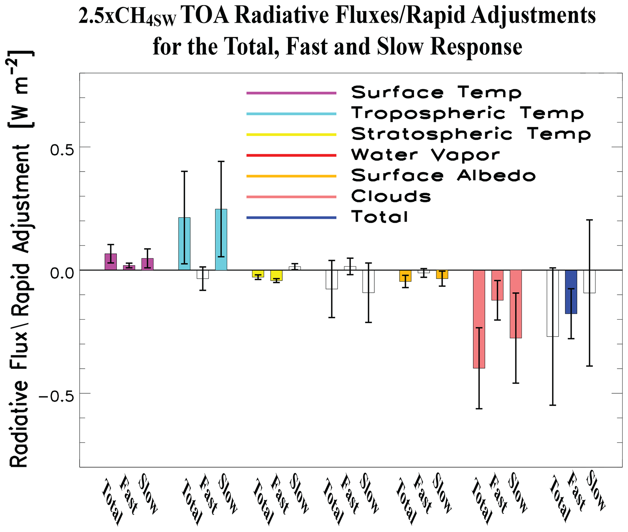
Figure 4 The 2.5xCH_4SW top-of-the-atmosphere radiative flux decomposition for the total response, fast response (rapid adjustment) and slow response. Global annual mean top-of-the-atmosphere (TOA) surface temperature (purple), tropospheric temperature (cyan), stratospheric temperature (yellow), water vapor (red), surface albedo (orange), cloud (pink) and total (blue) radiative flux decomposition for 2.5xCH_4SW. The total response (from the coupled ocean–atmosphere simulations) is represented by the first bar in each like-colored set of three bars, the rapid adjustment (fast response from fixed climatological sea surface temperature simulations) is represented by the second bar and the surface-temperature-induced response (slow response, estimated as the difference in the total response minus the fast response) is represented by the third bar. Uncertainty is quantified using the 90 % confidence interval; unfilled bars denote responses that are not significant at the 90 % confidence level (units: W m⁻²).

3.4 2.5xCH_4SW slow climate response

We apply the radiative kernel decomposition to the 2.5xCH_4SW coupled ocean–atmosphere simulation (Fig. 4; Fig. S4 shows the corresponding results for 2.5xCH_4SW+LW and 2.5xCH_4LW). The fast responses from the fixed climatological SST runs (i.e., the rapid adjustments) and the surface-temperature-induced slow responses (i.e., the difference between the coupled ocean–atmosphere and fixed climatological SST simulations) are also included. Here, a positive slow response has the same meaning as a positive fast response (ADJ), as both represent a net energy increase. Similarly, a negative slow response has the same meaning as a negative ADJ, as both represent a net energy decrease (i.e., we do not normalize by the change in surface air temperature, as is done to calculate a climate feedback). As with the larger methane perturbations, the cloud rapid adjustment and the cloud slow response under 2.5xCH_4SW are both negative at $-\mathrm{0.12}\pm \mathrm{0.08}$ W m⁻² and $-\mathrm{0.28}\pm \mathrm{0.18}$ W m⁻², respectively. Both are consistent with an increase in low-cloud cover (particularly the slow response at 0.31±0.25 %; Table S1). This implies that surface cooling in response to 2.5xCH_4SW radiative effects is largely due to the cloud rapid adjustment and cloud slow responses.

As mentioned in Sect. 3.1, the 2.5xCH_4SW stratospheric temperature adjustment under fixed climatological SSTs also significantly contributes (at $-\mathrm{0.04}\pm \mathrm{0.01}$ W m⁻², about 1/3 the magnitude of the cloud adjustment) to the total rapid adjustment. This negative stratospheric temperature adjustment is consistent with the relatively large increase in stratospheric shortwave heating (Fig. 2b) and warming (Fig. 2c), which results in enhanced outgoing longwave radiation (i.e., loss of energy and a negative adjustment). The tropospheric temperature adjustment (Fig. 4) is also negative but not significant at the 90 % confidence level, at $-\mathrm{0.03}\pm \mathrm{0.05}$ W m⁻². In contrast, the surface temperature adjustment at 0.02±0.01 W m⁻² (associated with cooling of the land surfaces and subsequent reduction in upwards longwave radiation) acts to weakly mute the negative total rapid adjustment. The other 2.5xCH_4SW rapid adjustment components (e.g., tropospheric temperature, water vapor, surface albedo) are relatively small and not significant at the 90 % confidence level.

In terms of the 2.5xCH_4SW slow response, in addition to the dominant negative contribution from clouds, the water vapor and surface albedo slow response also contribute to the negative total slow response at $-\mathrm{0.09}\pm \mathrm{0.12}$ and $-\mathrm{0.035}\pm \mathrm{0.03}$ W m⁻², respectively (Fig. 4). These are associated with tropospheric/surface cooling, resulting in less water vapor (a greenhouse gas) and enhanced snow/ice over land (enhanced albedo). In contrast, the tropospheric temperature and surface temperature slow responses are both significant and positive at 0.25±0.19 and 0.05±0.04 W m⁻², respectively, and act to mute the total negative slow response (the stratospheric temperature adjustment also weakly contributes to this muting, at 0.01±0.01 W m⁻²).

We note that the 2.5xCH_4SW total radiative flux decomposition (sum over clouds, water vapor, etc.) for the slow response is negative (opposite expectations since the surface cools). However, there is large uncertainty, i.e., it is a nonsignificant negative value at $-\mathrm{0.10}\pm \mathrm{0.30}$ W m⁻². This number is based on the corresponding difference between the coupled ocean–atmosphere total response and the rapid adjustment from the fSST simulation, which have values of $-\mathrm{0.27}\pm \mathrm{0.28}$ W m⁻² and $-\mathrm{0.16}\pm \mathrm{0.10}$ W m⁻², respectively. The former number ($-\mathrm{0.27}\pm \mathrm{0.28}$ W m⁻²) is based on the total radiative flux decomposition under 2.5xCH_4SW+LW minus 2.5xCH_LW, which have respective values of $-\mathrm{0.46}\pm \mathrm{0.18}$ W m⁻² and $-\mathrm{0.19}\pm \mathrm{0.19}$ W m⁻². So here, both values are negative, as expected (i.e., the system responds to the positive forcing by warming and emitting more energy into space, consistent with a stable climate system). It is likely that longer integrations (beyond 90 years) are necessary to reduce the relatively large uncertainty in some of these values.

Decomposing the 2.5xCH_4SW cloud rapid adjustment into shortwave and longwave radiation components (not shown), we find the cloud rapid adjustment for shortwave radiation is $-\mathrm{0.08}\pm \mathrm{0.08}$ W m⁻² and the cloud adjustment for longwave radiation is $-\mathrm{0.05}\pm \mathrm{0.03}$ W m⁻². Thus, both shortwave and longwave cloud radiative components contribute similarly to the negative cloud rapid adjustment. Decomposing the slow cloud response into shortwave and longwave radiation components, we find corresponding values of $-\mathrm{0.33}\pm \mathrm{0.17}$ and 0.05±0.05 W m⁻², respectively. Here, the negative cloud slow response is largely due to cloud shortwave radiative effects (consistent with the low-cloud increase of 0.31±0.25 %; Table S1), which is partially muted by cloud longwave radiative effects. These changes are qualitatively consistent with the 2.5xCH_4SW CLOUD changes discussed in Sect. 3.3, under the broad assumption that low clouds primarily reflect shortwave radiation and high clouds primarily inhibit outgoing longwave radiation. The 2.5xCH_4SW CLOUD changes under the fast response (Fig. 2e) are augmented in the upper troposphere (larger decreases in high-level cloud) compared to the total response (Fig. 3c) and in particular compared to the slow (Figs. S5c, S6d) response. The weaker decrease in upper-level clouds under the slow response is consistent with a lack of an increase in the upper-tropospheric shortwave heating rate (Fig. S6a). These statements are clearer under 10xCH_4SW (Figs. S5i, S7).

In contrast, CLOUD changes under the total response (and the slow response) are augmented in the low to middle troposphere (larger increases in low- to mid-level cloud) compared to the fast response. The larger increase in low-level cloud under the slow response (most of which occurs over marine stratocumulus regions off the North and South American western coasts; Fig. S5a, d, g, j) is consistent with a low-level cloud positive feedback i.e., surface cooling promotes more low clouds and in turn, more cooling, etc. (Clement et al., 2009; Zelinka et al., 2020).

To summarize, we find that the shortwave absorption associated with the present-day methane perturbation (2.5xCH₄) offsets 28 % (7 % to 55 %) of the surface warming associated with its longwave radiative effects. Similarly, although not significant, methane shortwave absorption associated with the present-day perturbation mutes 19 % of the positive ERF under methane longwave radiative effects, and 66 % of the precipitation increase is offset. These responses are associated with changes in the vertical profiles of shortwave heating (i.e., increases for pressures < 700 hPa and decreases for pressures > 700 hPa), which impact atmospheric temperature, relative humidity and cloud cover. Although some of the 2.5xCH_4SW results lack significance at the 90 % confidence level (e.g., the total precipitation response), they are qualitatively consistent with the results based on the larger 5xCH₄ and 10xCH₄ perturbations showed in A23 (where, for example, the total precipitation response is significant). The lack of more-significant signals under 2.5xCH_4SW is due to the weaker perturbation relative to internal climate variability. However, the consistency of the 2.5xCH_4SW signals relative to those under the larger methane perturbations (5xCH_4SW and 10xCH_4SW) supports the robustness of the main conclusions regarding the importance of methane SW absorption.

3.5 Additional analysis of the precipitation response

Precipitation responses can be understood from an energetic perspective (Muller and O'Gorman, 2011; Richardson et al., 2016; Liu et al., 2018). Precipitation is related to the diabatic cooling and the dry static energy flux divergence of the atmosphere as $L_{\mathrm{c}}P=Q+H$, where L_c is the latent heat of condensation of water vapor, P is precipitation, Q is the column-integrated diabatic cooling of the atmosphere excluding latent heating and H is the column-integrated dry static energy flux divergence. Q is estimated as LWC + SWC + SH. LWC is the net longwave radiative cooling of the atmosphere. SWC is the net shortwave radiative cooling of the atmosphere. The “C” stands for cooling, i.e., positive SWC and LWC represent cooling of the atmospheric column. In CESM2, positive longwave radiative fluxes are upwards, so LWC is calculated as the net LW radiation at the TOA minus that at the surface. In CESM2, positive shortwave radiative fluxes are downwards, so SWC is calculated as the net SW radiation at the surface minus the net SW radiation at the TOA (or equivalently, the negative of the net SW radiation at TOA minus that at the surface). Both terms are positive for cooling (energy loss). SH is the downwards sensible heat flux at the surface (i.e., positive values indicate atmospheric cooling). H is estimated as the residual between L_cP and Q. In the global mean, the circulation term (i.e., H) is zero, implying L_cP=Q. As Q is composed of LWC and SWC (and SH but it is generally small), this balance shows that condensational heating via precipitation is largely balanced by radiative cooling of the atmosphere. An increase in atmospheric SW absorption (e.g., via CH_4SW) will decrease atmospheric radiative cooling and decrease precipitation in turn.

Figure 5a, b show the atmospheric energy budget decomposition for the total, fast and slow responses under 10xCH_4SW and 2.5xCH_4SW. Under both CH_4SW perturbations, the decrease in global mean precipitation (i.e., the energy of precipitation L_cP) is dominated by the slow response. For example, under 2.5xCH_4SW, L_cP decreases by $-\mathrm{0.09}\pm \mathrm{0.09}$ W m⁻² under the fast response. This increases (in magnitude) to $-\mathrm{0.15}\pm \mathrm{0.30}$ W m⁻² under the slow response (i.e., total decrease is $-\mathrm{0.24}\pm \mathrm{0.28}$ W m⁻²). Although these 2.5xCH_4SW changes are not significant at the 90 % confidence level, all three L_cP decreases are significant under 10xCH_4SW at $-\mathrm{0.29}\pm \mathrm{0.10}$, $-\mathrm{0.83}\pm \mathrm{0.27}$ and 1.12±0.25 W m⁻², respectively. The precipitation decrease under the slow response is largely associated with a decrease in net longwave atmospheric radiative cooling (i.e., LWC) of $-\mathrm{0.17}\pm \mathrm{0.34}$ W m⁻² for 2.5xCH_4SW and 1.03±0.32 W m⁻² for 10xCH_4SW (i.e., anomalous longwave radiative warming), which is consistent with cooling of the troposphere (e.g., Figs. S6b and S7b). The decrease in net longwave atmospheric radiative cooling under the slow response is weakly muted by an increase in net shortwave radiative cooling at 0.03±0.08 W m⁻² for 2.5xCH_4SW and 0.30±0.09 W m⁻² for 10xCH_4SW (i.e., anomalous shortwave radiative cooling), consistent with tropospheric cooling and decreases in atmospheric water vapor (i.e., specific humidity decreases throughout the troposphere under the slow response; Figs. S6f and S7f). This yields less solar absorption by water vapor, i.e., QRS decreases in the middle and upper troposphere under the slow response (Figs. S6a and S7a).

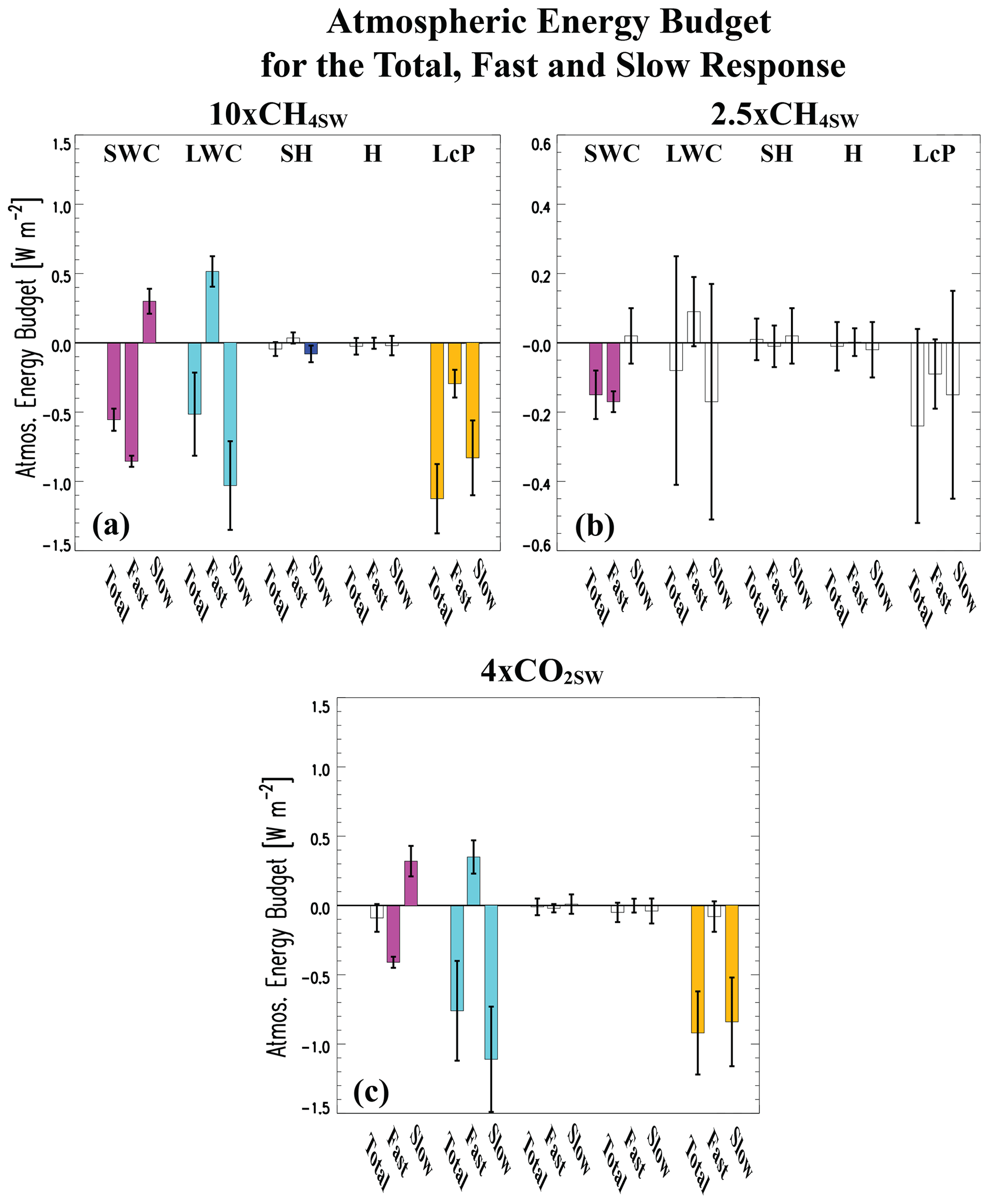
Figure 5 Atmospheric energy budget decomposition for the total, fast and slow responses. Annual mean global mean energy budget decomposition for (a) 10xCH_4SW; (b) 2.5xCH_4SW and (c) 4xCO_2SW. Components include net shortwave radiative cooling from the atmospheric column (SWC), net longwave radiative cooling from the atmospheric column (LWC), net downwards sensible heat flux at the surface (SH) and column-integrated dry static energy flux divergence (H). Positive values indicate cooling (energy loss). Also included is total latent heating (L_cP). The sum of the first four terms is equal to the last term (L_cP). The total response (from the coupled ocean–atmosphere simulations) is represented by the first bar in each like-colored set of three bars, the rapid adjustment (fast response from fixed climatological sea surface temperature simulations) is represented by the second bar and the surface-temperature-induced response (slow response, estimated as the difference in the total response minus the fast response) is represented by the third bar. Uncertainty is quantified using the 90 % confidence interval; unfilled bars denote responses that are not significant at the 90 % confidence level (units: W m⁻²). Note the different y axis in panel (b).

The CH_4SW decrease in L_cP under the fast response is associated with opposite changes in SWC and LWC, including dominance of the SWC term as opposed to the LWC term. This includes an SWC decrease of $-\mathrm{0.18}\pm \mathrm{0.03}$ W m⁻² for 2.5xCH_4SW and $-\mathrm{0.85}\pm \mathrm{0.04}$ W m⁻² for 10xCH_4SW (i.e., less shortwave radiative cooling), which is consistent with the enhanced solar absorption by CH_4SW under the fast response (e.g., Figs. S6a and S7a). This is partially offset by an increase in LWC, consistent with middle- to upper-tropospheric warming and enhanced outgoing longwave radiation.

The L_cP decrease under the total response is associated with similar magnitude decreases in both SWC and LWC. This is particularly true for 10xCH_4SW, where the SWC term decreases by $-\mathrm{0.55}\pm \mathrm{0.08}$ W m⁻² and the LWC term decreases by $-\mathrm{0.51}\pm \mathrm{0.30}$ W m⁻². Under 2.5xCH_4SW, the corresponding changes are $-\mathrm{0.15}\pm \mathrm{0.07}$ and $-\mathrm{0.08}\pm \mathrm{0.33}$ W m⁻², respectively. In all cases, the H term is near zero in the global mean (i.e., energy transport in the global mean should be zero). Similarly, the SH term is generally small in all cases.

To summarize these results, the decrease in global mean precipitation under CH_4SW is associated with both the fast and slow responses, with most of the precipitation decrease related to the slow (surface temperature mediated) response. The decrease in precipitation under the fast response is largely due to the enhanced solar absorption by CH_4SW (decrease in the SWC term above), i.e., as atmospheric solar absorption increases, net atmospheric radiative cooling decreases, which leads to a decrease in precipitation. In contrast, the decrease in precipitation under the slow response is largely due to cooling of the troposphere and a decrease in net longwave atmospheric radiative cooling (decrease in the LWC term above).

The importance of both the fast and slow responses (and the dominance of the slow response) in driving less global mean precipitation under CH_4SW is in contrast to other shortwave absorbers such as black carbon. With idealized black carbon perturbations, for example, the fast and slow global mean precipitation responses oppose one another. The fast response (associated with black carbon atmospheric solar absorption) yields a global mean decrease in precipitation, whereas the weaker slow response (associated with surface warming) yields an increase in global mean precipitation (Samset et al., 2016; Stjern et al., 2017). The net result is a decrease in global mean precipitation, largely due to the fast response and enhanced atmospheric solar absorption by black carbon.

This difference in behavior between BC and CH_4SW is because BC has a positive TOA ERF, whereas CH_4SW has a negative TOA ERF. The positive TOA ERF under BC acts to warm the surface, which promotes an increase in precipitation under the slow response. The negative TOA ERF under CH_4SW acts to cool the surface (as shown here), which promotes a decrease in precipitation under the slow response. However, both BC and CH_4SW have a positive atmospheric ERF (which promotes less precipitation via fast adjustments).

Thus, the main difference between the black carbon and CH_4SW impact on global mean precipitation is related to the slow response. Black carbon warms the surface, which mutes the overall decrease in global mean precipitation (from the fast response). In contrast, CH_4SW cools the surface, which adds to the overall decrease in global mean precipitation (and contributes more to the decrease than the fast response does).

We further decompose the global mean precipitation response based on the equation $L_{\mathrm{c}}\mathrm{\Delta }P=\mathrm{A}+\mathit{\eta }\mathrm{\Delta }$TAS (e.g., Fläschner et al., 2016) where L_c is defined as above and equal to 29 W m⁻² (mm d${}^{-\mathrm{1}}{)}^{-\mathrm{1}}$; ΔP is the change in the global mean precipitation (mm d⁻¹); ΔTAS is the change in global mean near-surface air temperature (K); A is an adjustment term (estimated from our fSST experiments) that accounts for the change in precipitation independent of any change in surface temperature (W m⁻²), which can be further decomposed into SWC+LWC+SH where SWC is the net shortwave radiative cooling of the atmosphere as defined above (W m⁻²); LWC is the net longwave radiative cooling of the atmosphere as defined above (W m⁻²); and SH is the downwards sensible heat flux at the surface (W m⁻²) (positive values for these three terms indicate cooling and energy loss as defined above). The hydrological sensitivity parameter is η (W m⁻² K⁻¹).

Table S3 (and Fig. S8) shows that the hydrological sensitivity parameter is always larger (in magnitude) under the various SW+LW signals (e.g., 2.5xCH_4LW+SW) compared to the LW-only signal (e.g., 2.5xCH_4LW). The SW signal consistently (outside of 2.5xCH_4SW) yields the smallest η. However, η has a relatively large uncertainty, and it is not significantly different between the various SW+LW signals and the corresponding LW-only signals. For example, the hydrological sensitivity parameter is 2.47±0.24 W m⁻² K⁻¹ for 10xCH_4LW+SW and 2.39±0.16 W m⁻² K⁻¹ for 10xCH_4LW. The corresponding value for 10xCH_4SW is 2.24±0.73 W m⁻² K⁻¹. Thus, although there are systematic differences, the hydrological sensitivity parameter is not significantly different under the LW-only effects versus SW effects of CH₄.

3.6 Comparisons with CO_2SW

In addition to CH₄, other greenhouse gases (GHGs), including carbon dioxide (CO₂), also absorb solar radiation. As with most climate models, CESM2 (via RRTMG) includes a representation of CO₂ SW absorption. In particular, RRTMG includes CO₂ SW absorption in four NIR/mid-IR bands: 1.3–1.6 µm, 1.9–2.15 µm, 2.5–3.1 µm and 3.8–12.2 µm. As mentioned above, RRTMG underestimates CO₂ SW IRF by 25 %–45 % (Hogan and Matricardi, 2020).

Prior studies (focused on the radiative forcing) have shown that the SW absorption effects of the present-day CO₂ perturbation are relatively small (Myhre et al., 1998; Etminan et al., 2016; Shine et al., 2022). For example, from the perspective of the SARF at the tropopause, CO₂ SW absorption yields a negative forcing that acts to decrease the magnitude of the CO₂ LW forcing by about 5 % (Myhre et al., 1998; Etminan et al., 2016). This is largely due to direct SW absorption in the stratosphere dominating over relatively weak increases in tropospheric SW absorption due to overlap with water vapor (Etminan et al., 2016). The former acts to decrease downwards SW at the tropopause (leading to a negative contribution that dominates the net effect), whereas the latter decreases upwards SW at the tropopause (leading to a smaller, positive forcing). The direct SW absorption in the stratosphere, by reducing LW cooling, also affects the temperature adjustment (i.e., the LW flux from the stratosphere to the troposphere is increased). As shown by Etminan et al. (2016), the overall negative contribution due to CO_2sw is due to the dominance of its 2.7 µm band. In contrast, for CH_4sw, the overall positive SW forcing is due to both its 1.7 and 2.3 µm bands. This contrasting behavior between CO_2SW and CH_4SW is largely driven by the amount of overlap of the SW absorption bands with the near-IR absorption bands for water vapor (Etminan et al., 2016).

To gain a better understanding of the importance of the SW absorption effects due to CH₄ relative to CO₂, we repeat our suite of CESM2 experiments but based on idealized CO₂ perturbations, including 2x and 4x preindustrial atmospheric CO₂ concentrations. This includes two sets of identical experiments (e.g., Table 1): one that includes CO₂LW + SW radiative effects (e.g., 2xCO${}_{\mathrm{2}}^{\mathrm{EXP}}$) and one that lacks CO₂ SW radiative effects (e.g., 2xCO${}_{\mathrm{2}\mathrm{NOSW}}^{\mathrm{EXP}}$). CO₂ SW absorption in the four NIR/mid-IR bands in RRTMG is turned off in the simulations that lack CO₂ SW radiative effects. These are compared to the default preindustrial control experiment (PIC^EXP), which includes CO₂ (and CH₄) LW + SW radiative effects, as well as to a new preindustrial control experiment with CO₂ SW radiative effects turned off (i.e., LW effects only, denoted as ${\mathrm{PIC}}_{\mathrm{NOCO}\mathrm{2}\mathrm{SW}}^{\mathrm{EXP}}$). As with the methane perturbations, this suite of CO₂ simulations allows quantification of the CO₂ LW + SW, LW and SW radiative effects, denoted, for example, as 2xCO_2LW+SW, 2xCO_2LW and 2xCO_2SW. The 2xCO_2LW+SW signal is obtained by subtracting the default 2xCO₂ perturbation from the default control (2xCO${}_{\mathrm{2}}^{\mathrm{EXP}}$ − PIC^EXP). The 2xCO_2LW signal is obtained by subtracting the 2xCO₂ perturbation without CO₂ SW absorption from the corresponding control simulation without CO₂ SW absorption ($\mathrm{2}{\mathrm{xCO}}_{\mathrm{2}\mathrm{NOSW}}^{\mathrm{EXP}}$ − ${\mathrm{PIC}}_{\mathrm{NOCO}\mathrm{2}\mathrm{SW}}^{\mathrm{EXP}}$). The 2xCO_2SW signal is obtained by taking the double difference, i.e., $(\mathrm{2}{\mathrm{xCO}}_{\mathrm{2}}^{\mathrm{EXP}}$ − PIC^EXP) − (2xCO${}_{\mathrm{2}\mathrm{NOSW}}^{\mathrm{EXP}}$ − ${\mathrm{PIC}}_{\mathrm{NOCO}\mathrm{2}\mathrm{SW}}^{\mathrm{EXP}}$).

We note here that it is difficult to directly compare our CH₄ and CO₂ results. For example, 2.5xCH₄ represents an increase of ∼ 0.0012 ppm, whereas 2xCO₂ represents an increase of ∼ 560 ppm. Nonetheless, we provide a qualitative comparison below.

Figure 6 shows the corresponding TOA radiative fluxes and rapid adjustments for both 2xCO₂ and 4xCO₂ (Fig. S9 shows the 4xCO_2SW radiative flux decompositions for the total, fast and slow responses). As expected, these perturbations yield a large positive TOA LW IRF at 2.59±0.05 W m⁻² for 2xCO₂ and 5.30±0.05 W m⁻² for 4xCO₂. The corresponding TOA SW IRFs are also positive, but they are much smaller at 0.03±0.05 and 0.05±0.05 W m⁻², respectively. The total rapid adjustment for both CO₂ perturbations is negative under SW radiative effects at $-\mathrm{0.06}\pm \mathrm{0.08}$ W m⁻² for 2xCO₂ and $-\mathrm{0.40}\pm \mathrm{0.09}$ W m⁻² for 4xCO₂. The larger negative total ADJ offsets the less-positive IRF, leading to a negative ERF at $-\mathrm{0.03}\pm \mathrm{0.15}$ W m⁻² for 2xCO_2SW and $-\mathrm{0.35}\pm \mathrm{0.15}$ W m⁻² for 4xCO_2SW (only the latter is significant at the 90 % confidence level). We reiterate that these negative values are due to isolation of CO₂ shortwave absorption alone; CO₂'s longwave effects still dominate the total rapid adjustment and ERF. Recall that under CH₄, the shortwave effects dominate the total SW+LW rapid adjustment but not the ERF (Fig. 1).

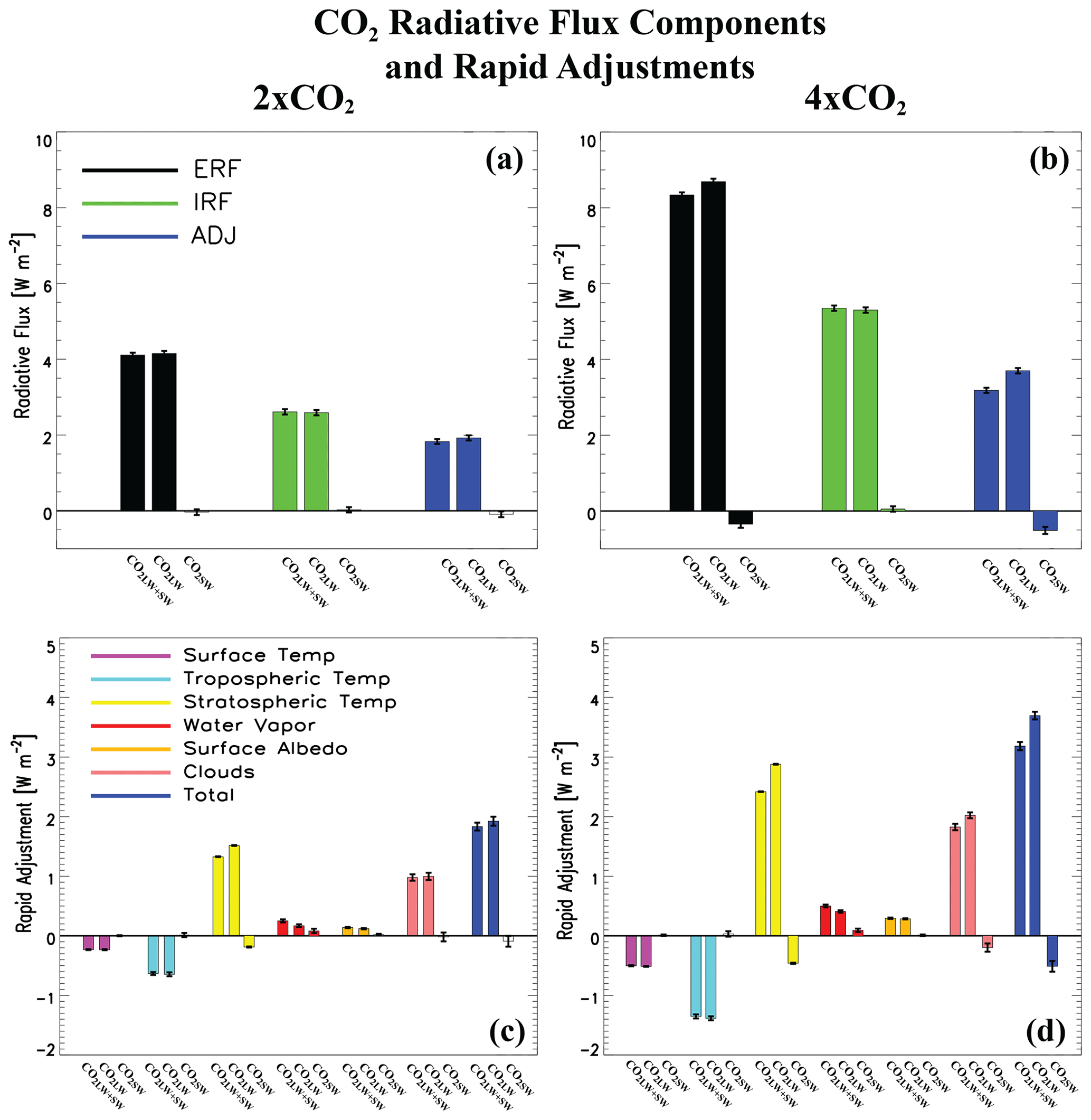
Figure 6 The 2xCO₂ and 4xCO₂ top-of-the-atmosphere radiative flux components and rapid adjustments. Global annual mean TOA (a, b) effective radiative forcing (ERF; black), instantaneous radiative forcing (IRF; green) and rapid adjustment (ADJ; blue) and (c, d) decomposition of the rapid adjustment into its components including surface temperature (purple), tropospheric temperature (cyan), stratospheric temperature (yellow), water vapor (red), surface albedo (orange), cloud (pink) and total rapid adjustment (blue) for (a, c) 2xCO₂ and (b, d) 4xCO₂. Responses are decomposed into CO₂ longwave and shortwave radiative effects (CO_2LW+SW), CO₂ longwave radiative effects (CO_2LW), and CO₂ shortwave radiative effects (CO_2SW). ERF and rapid adjustments are based on 30-year fixed climatological sea surface temperature simulations. Uncertainty is quantified using the 90 % confidence interval; unfilled bars denote responses that are not significant at the 90 % confidence level (units are W m⁻²).

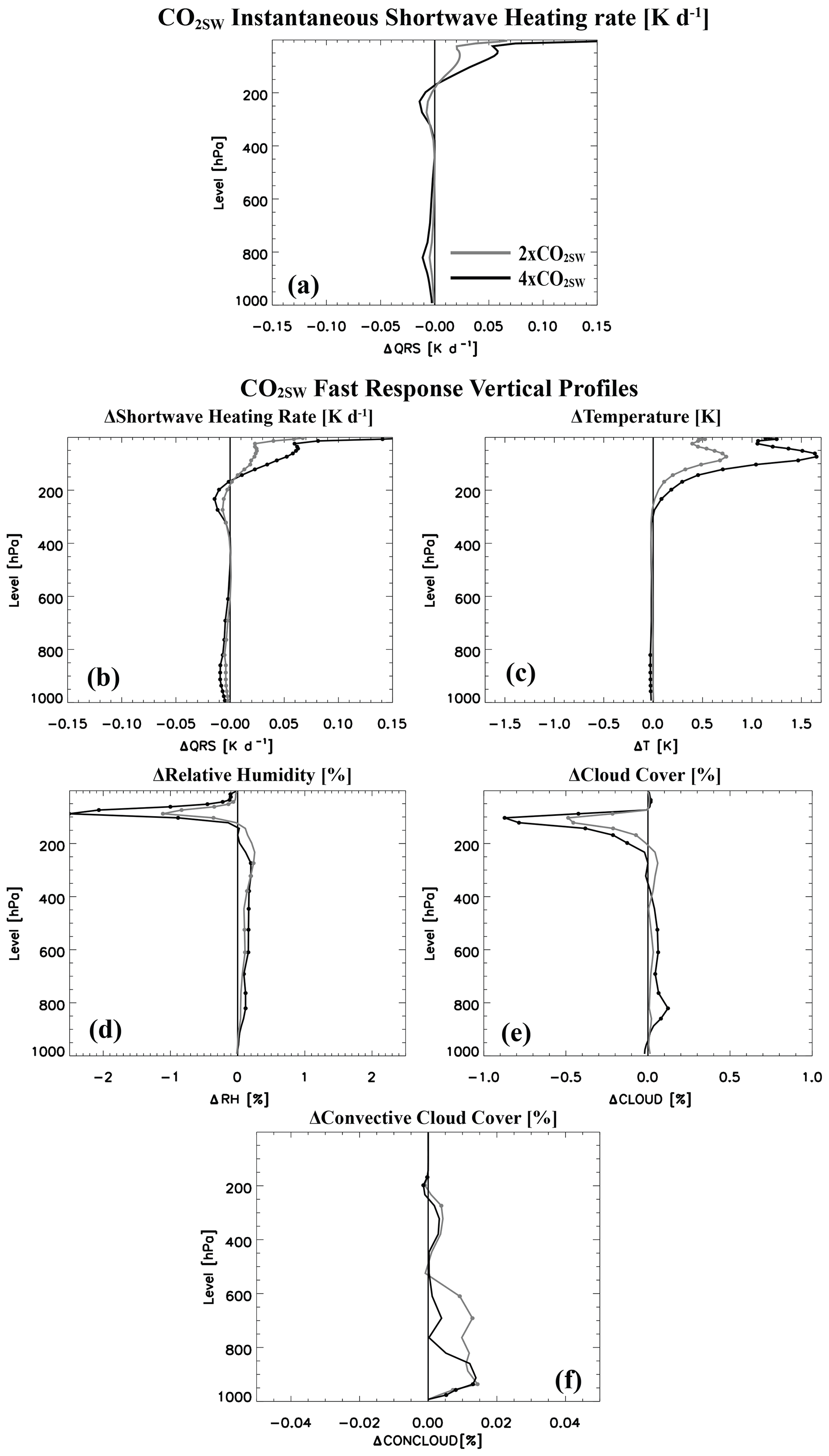
Figure 7 Global mean annual mean vertical-response profiles for two CO_2SW perturbations. Instantaneous (a) shortwave heating rate (QRS; units are K d⁻¹) and (b–f) fast responses of (b) QRS (units are K d⁻¹), (c) air temperature (T; units are K), (d) relative humidity (RH; units are %), (e) cloud cover (CLOUD; units are  %) and (f) convective cloud cover (CONCLOUD; units are %) for 2xCO_2SW (gray) and 4xCO_2SW (black). A significant response at the 90 % confidence level based on a standard t test is denoted by solid dots in (b–f). Climatologically fixed SST simulations are used to estimate the fast responses. Instantaneous QRS profiles come from the Parallel Offline Radiative Transfer Model (PORT).

These results are qualitatively consistent with 2.5xCH_4SW (Fig. 1), including a negative ADJ that offsets the positive IRF, leading to a negative ERF. The methane SW radiative effect, however, represents a larger percentage of its LW radiative effect. As discussed above, CH_4SW offsets ∼ 20 % of the positive ERF associated with CH_4LW (although it is not significant under 2.5xCH₄). This is due to a relatively strong negative rapid adjustment associated with CH_4SW (e.g., $-\mathrm{0.16}\pm \mathrm{0.10}$ W m⁻² for 2.5xCH_4SW, which increases to $-\mathrm{0.77}\pm \mathrm{0.11}$ W m⁻² for 10xCH_4SW). This, in turn, drives the negative CH_4SW ERF.

In contrast, 2xCO_2SW and 4xCO_2SW offset only 0.7 % and 4 % (only the latter is significant at the 90 % confidence level) of the positive ERF associated with their LW radiative effects, respectively. The weaker CO_2SW muting of CO_2LW ERF is related to a relatively weak CO_2SW negative adjustment ($-\mathrm{0.06}\pm \mathrm{0.08}$ W m⁻² for 2xCO_2SW but increasing to $-\mathrm{0.40}\pm \mathrm{0.09}$ W m⁻² for 4xCO_2SW) that leads to a relatively weak negative CO_2SW ERF. The weaker CO_2SW muting of CO_2LW ERF is also related to the relatively large and positive CO_2LW ERF. This large and positive CO_2LW ERF is due to a relatively large and positive ADJ under CO_2LW (largely due to the stratospheric temperature adjustment, as well as clouds; Fig. 6) that reinforces the relatively large and positive CO_2LW IRF. For example, 2xCO_2LW yields an ADJ of 1.55±0.08 W m⁻² and a corresponding ERF of 4.15±0.10 W m⁻². Thus, the weaker CO_2SW muting of CO_2LW ERF is related to a relatively weak SW radiative effect, particularly compared to its very strong LW radiative effect.

We also note that the negative total rapid adjustment due to CO₂ SW absorption is dominated by a negative stratospheric temperature adjustment (Fig. 6c, d). This is also in contrast to methane, where clouds (followed by the stratospheric temperature adjustment) drive most of the negative total rapid adjustment under SW radiative effects (Fig. 1b). For 4xCO_2SW, the stratospheric adjustment is $-\mathrm{0.46}\pm \mathrm{0.01}$ W m⁻² compared to $-\mathrm{0.19}\pm \mathrm{0.07}$ W m⁻² for clouds. This larger negative stratospheric adjustment under 4xCO_2SW is consistent with relatively large shortwave heating above ∼ 200 hPa (to be discussed below).

The ERF, IRF and ADJ under 2xCO₂ LW + SW radiative effects shown here compare well with those from PDRMIP (Smith et al., 2018), although CESM2 yields a larger positive ADJ (and ERF). For example, PDRMIP yields a multi-model mean IRF, ERF and ADJ of ∼ 2.5, 3.7 and 1.2 W m⁻², respectively. The corresponding values from our 2xCO₂ CESM2 simulation are 2.6±0.06, 4.1±0.11 and 1.6±0.07 W m⁻². The bulk of CESM2's larger ADJ is due to a larger cloud adjustment at 0.98±0.05 W m⁻² compared to 0.45 W m⁻² for PDRMIP.

Figure 7a shows the global mean instantaneous shortwave heating rate profile for 2xCO_2SW and 4xCO_2SW. Both profiles show a decrease in QRS throughout the troposphere with two minima: one near 800 hPa in the lower troposphere and another near 250 hPa in the upper troposphere. Above 200 hPa, QRS increases rapidly through the stratosphere, reaching ∼ 0.15 K d⁻¹ at 3.6 hPa under 4xCO_2SW. The vertical structure of QRS under CO_2SW shows similarities to that under CH_4SW (Fig. 2a), but CO_2SW exhibits QRS decreases throughout the entire troposphere as well as relatively large QRS increases in the stratosphere. In other words, the transition level from decreasing to increasing QRS occurs higher aloft under CO_2SW, with larger QRS increases in the stratosphere.

The corresponding fSST fast responses are included in Fig. 7b–f. The QRS profile (Fig. 7b) is very similar to the corresponding instantaneous profile (Fig. 7a). The relatively large CO_2SW stratospheric solar heating helps to explain the correspondingly large negative stratospheric temperature adjustment (Fig. 6c, d). That is, the large increase in stratospheric solar absorption leads to corresponding warming and subsequently to enhanced outgoing longwave radiation that acts to cool the climate system. The decrease in tropospheric QRS is associated with weak cooling (Fig. 7c) and increases in both relative humidity (Fig. 7d) and clouds (Fig. 7e), with stronger responses under 4xCO_2SW compared to 2xCO_2SW. The opposite responses occur in the stratosphere. These results again share similarities to those based on CH_4SW (Fig. 2), but CO_2SW exhibits more uniform changes throughout the troposphere (i.e., the transition level occurs higher aloft), as well as relatively large stratospheric changes.

Due to the relatively weak and non-significant 2xCO_2SW radiative fluxes (and limited computational resources), we only perform the coupled ocean–atmosphere simulations for 4xCO₂. Figure 8a–c show the global mean total, fast and slow response vertical profiles under 4xCO_2SW for QRS, temperature and cloud cover. Significant cooling (Fig. 8b) occurs under the total (and slow) response throughout the troposphere, with maximum cooling of ∼ 0.5 K near 200 hPa under the total response. Above this level, cooling gradually weakens and transitions into warming aloft, peaking at ∼ 1 K near 50 hPa. The corresponding vertical CLOUD total response profile (Fig. 8c) shows increasing cloud cover throughout the troposphere, with decreases aloft (near 100 hPa) generally similar to the fast response but with larger tropospheric CLOUD increases and weaker CLOUD decreases aloft. The global maps of the TAS and P total climate response under 4xCO_2SW are included in Fig. 8 d, e. The 4xCO_2SW drives a significant decrease in TAS and P at $-\mathrm{0.38}\pm \mathrm{0.12}$ K and $-\mathrm{0.031}\pm \mathrm{0.01}$ mm d⁻¹ (−1.05 %).

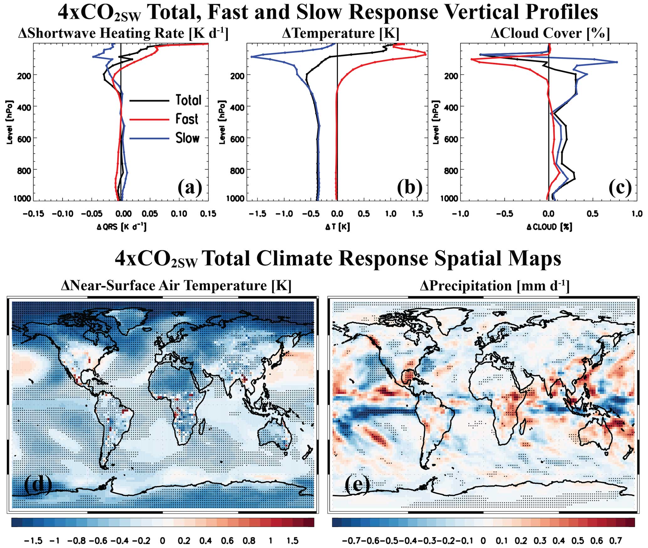
Figure 8 The 4xCO_2SW responses. The 4xCO_2SW annual mean global mean vertical-response profiles of (a) shortwave heating rate (QRS; units are K d⁻¹), (b) air temperature (T; units are K) and (c) cloud cover (CLOUD; units are  %) for the total (black), fast (red) and slow (blue) responses. Also included are 4xCO_2SW global maps of the annual mean (d) near-surface air temperature (K) and (e) precipitation (mm d⁻¹) change for the total climate response. A significant response at the 90 % confidence level based on a standard t test is denoted by solid dots. Total climate responses are estimated from coupled ocean–atmosphere CESM2 simulations.

Table S2 (and Fig. S3d) shows the individual components of the TOA energy decomposition equation, including the estimated climate feedback parameter, for the 4xCO₂ simulations. As with the methane signals, the climate feedback parameter is larger (in magnitude) under 4xCO_2LW+SW compared to 4xCO_2LW but not significantly so. For example, α is $-\mathrm{1.18}\pm \mathrm{0.06}$ W m⁻² K⁻¹ for 4xCO_2LW+SW and $-\mathrm{1.11}\pm \mathrm{0.06}$ W m⁻² K⁻¹ for 4xCO_2LW. The corresponding α value for 4xCO_2SW is $-\mathrm{0.31}\pm \mathrm{0.93}$ W m⁻² K⁻¹.

Under 4xCO_2SW, the TAS and P responses are quite small compared to the corresponding LW radiative effects at 5.84±0.08 K and 0.27±0.01 mm d⁻¹ (9.1 %), respectively. For example, if CH_4LW yielded the same 5.84 K of warming, this would correspond to surface cooling associated with CH_4SW of ∼ 1.75 K (assuming 30 % offset, which may not apply here). In terms of TAS, 4xCO_2SW mutes 6.5 % of the warming due to LW radiative effects. For P, 4xCO_2SW mutes 11.5 % of the increase in precipitation due to LW radiative effects. Thus, the muting effects of CO_2SW are much weaker than those associated with CH_4SW, where ∼ 30 % of the warming and ∼ 60 % of the wetting due to CH₄ LW radiative effects are offset.

We also perform the atmospheric energy balance calculation (Sect. 3.5) on the suite of 4xCO_2SW simulations (Fig. 5c). Overall, the conclusions discussed in Sect. 3.5 under 2.5xCH_4SW and 10xCH_4SW also apply under 4xCO_2SW. The decrease in the global mean energy of precipitation under 4xCO_2SW ($-\mathrm{0.91}\pm \mathrm{0.30}$ W m⁻² under the total response) is associated with both the fast response (a non-significant decrease of $-\mathrm{0.08}\pm \mathrm{0.11}$ W m⁻²) and the slow responses ($-\mathrm{0.83}\pm \mathrm{0.32}$ W m⁻²). Here, nearly all of the precipitation decrease (91 % as opposed to 63 % for 2.5xCH_4SW and 74 % for 10xCH_4SW) is related to the slow (surface-temperature-mediated) response. In other words, only 9 % of the precipitation decrease under 4xCO_2SW is due to the fast response, which is much lower than that under CH_4SW (26 %–37 %). The weaker contribution to the decrease in total precipitation by the 4xCO_2SW fast response is consistent with similar (but opposite-signed) changes in the SWC and LWC terms at $-\mathrm{0.41}\pm \mathrm{0.04}$ W m⁻² and 0.35±0.12 W m⁻², respectively, which neutralize one another. This cancellation is consistent with the 4xCO_2SW solar heating profile (e.g., Fig. 7b), where nearly all of the heating occurs in the stratosphere. Thus, the added solar heating – although decreasing the SWC term – primarily warms the stratosphere where the energy is efficiently radiated back into space (i.e., the SWC decrease is primarily balanced by an increase in the LWC term). This is in contrast to the QRS profiles under CH_4SW (e.g., Fig. 2b), which show significant solar absorption throughout the middle and upper troposphere (pressures < 700 hPa). Thus, we suggest the relatively weak decrease in precipitation under the 4xCO_2SW fast response (relative to the CH_4SW perturbations) is related to differences in the vertical QRS profile, with CO_2SW solar absorption primarily occurring in the stratosphere.

Table S3 (and Fig. S8d) shows the individual components of the alternate precipitation energy decomposition equation, including the estimated hydrological sensitivity parameter, for the 4xCO₂ simulations. For example, η is 2.47±0.04 W m⁻² K⁻¹ for 4xCO_2LW+SW and 2.46±0.04 W m⁻² K⁻¹ for 4xCO_2LW. The corresponding η value for 4xCO_2SW is smaller (but not significantly so, as with methane), at 2.31±0.89 W m⁻² K⁻¹. Thus, similar to the methane simulations, although there are systematic differences, we do not find significant differences between the hydrological sensitivity parameter under the LW-only effects versus the SW effects of CO₂.

3.7 Climate feedbacks

As discussed above, the climate feedback parameter (as estimated via a regression approach; Table S2) is always larger (in magnitude) under the various SW+LW signals (e.g., 2.5xCH_4LW+SW) compared to the LW-only signal (e.g., 2.5xCH_4LW). Although these differences are not significant, they suggest that the climate system does not have to warm as much to offset the same TOA energy imbalance when SW effects are included. We perform an alternate procedure to calculate the total climate feedback and its components by normalizing the slow response's radiative flux decomposition (based on the radiative kernel method) by the corresponding change in global mean near-surface air temperature. Figure 9 shows the corresponding feedback decomposition. We first point out that the total climate feedback as calculated here (α_k) is similar (i.e., error bars overlap except for 4xCO₂) to that previously estimated using the regression approach (α; Table S2). Thus, α_k is also always larger (in magnitude) under the various SW+LW signals compared to the corresponding LW-only signals, with consistently smaller (negative) magnitudes under the SW-only signals (outside of 2.5xCH_4SW). Although α_k has smaller uncertainty (compared to α), these differences continue to lack significance (i.e., the blue bar's errors overlap in Fig. 9). It is also clear, however, that the individual feedbacks (e.g., tropospheric temperature feedback) are all very similar across CH₄ and CO₂ LW + SW, LW, and SW radiative effects – except the cloud feedback, where significant differences exist (for the larger perturbations). For example, the cloud feedback is 0.05±0.20 W m⁻² K⁻¹ for 10xCH_4LW+SW, 0.36±0.09 W m⁻² K⁻¹ for 10xCH_4LW and 1.0±0.53 W m⁻² K⁻¹ for 10xCH_4SW (i.e., the cloud feedback is significantly different between SW versus LW radiative effects; Fig. 9a). Thus, the larger (positive) cloud feedback under SW radiative effects acts to weaken the total (negative) feedback, which helps to explain the previously mentioned systematically smaller (in magnitude) values for α (and α_k) under SW effects. Furthermore, the systematically larger (negative) values for α and α_k under SW+LW effects is due to a relatively weak cloud feedback (e.g., 0.05±0.20 W m⁻² K⁻¹ for 10xCH_4LW+SW). We also clarify here that this weak cloud feedback under SW+LW effects is due to the fact that LW effects are associated with surface warming and decreased low-cloud cover under the slow response (Table S1), which in turn drives more warming (i.e., a positive cloud feedback). This is weakened by SW effects, which are associated with surface cooling and increased low-cloud cover under the slow response (Table S1), which in turn drives more cooling (i.e., a positive feedback that opposes that under LW effects). Even though the surface cooling under SW effects is relatively small compared to the warming under LW effects, the cloud feedback under SW effects is larger than that under LW effects, effectively leading to a smaller cloud feedback under SW+LW effects (and not significant under all of the CH₄ perturbations). The net effect is that the planet does not need to warm up as much under SW+LW effects to restore the energy balance due to the SW effects on clouds under the slow response (and in particular, increased low clouds; Table S1). Analogously, these results imply relatively large cooling per unit of forcing under methane shortwave radiative effects, which in turns leads to relatively less warming per unit forcing under methane shortwave and longwave radiative effects.

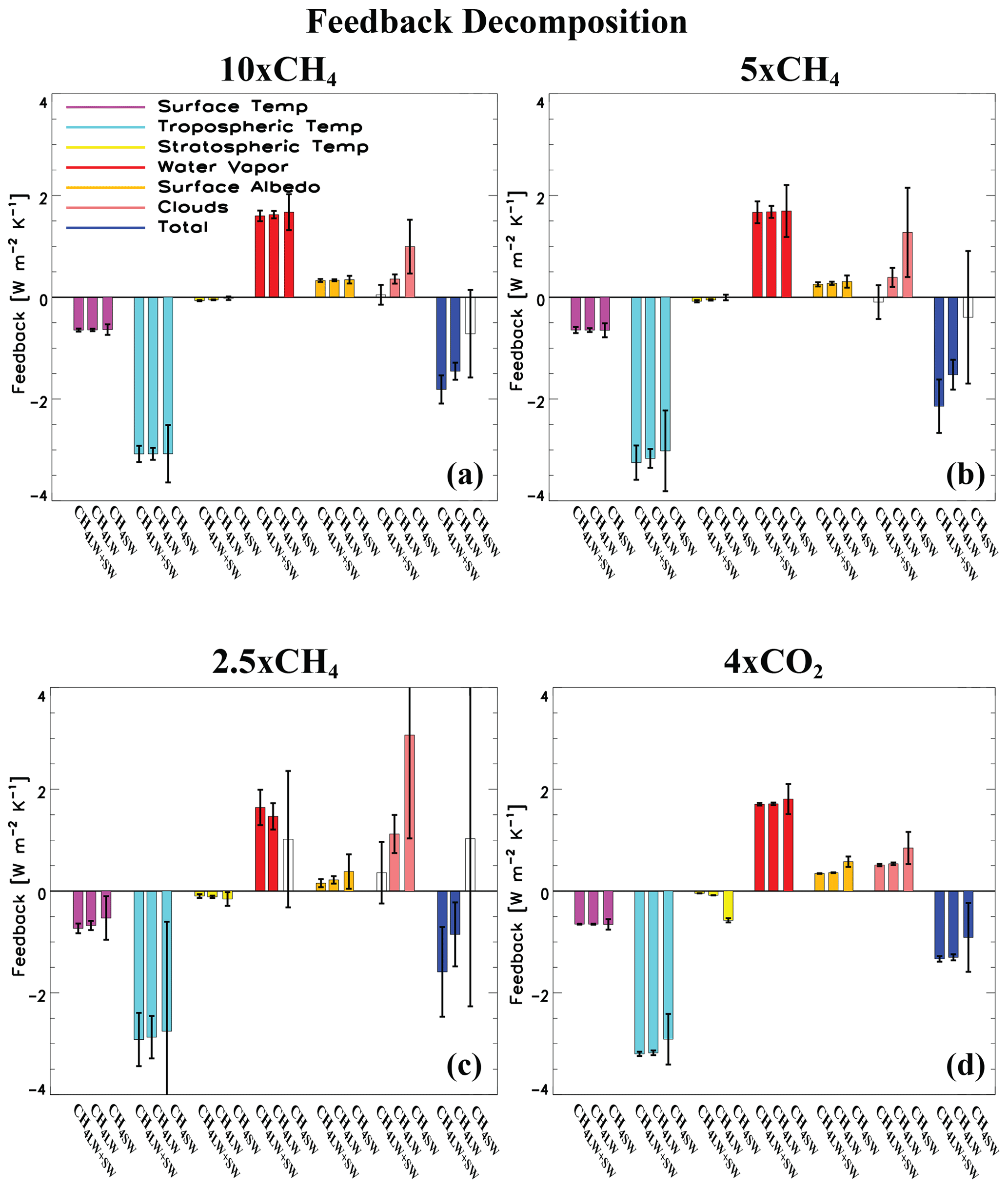
Figure 9 Feedback decomposition based on the radiative kernel method. Global annual mean top-of-the-atmosphere (TOA) surface temperature (purple), tropospheric temperature (cyan), stratospheric temperature (yellow), water vapor (red), surface albedo (orange), cloud (pink) and total (blue) feedback decomposition, as estimated by normalizing the slow response's radiative flux decomposition by the corresponding change in global mean near-surface air temperature. Feedbacks are decomposed into CH₄ and CO₂ longwave and shortwave radiative effects (e.g., CH_4LW+SW; first bar in each like-colored set of three bars), longwave radiative effects (e.g., CH_4LW; second bar) and shortwave radiative effects (e.g., CH_4SW; third bar). Uncertainty is quantified using the 90 % confidence interval; unfilled bars denote responses that are not significant at the 90 % confidence level (units: W m⁻² K⁻¹).

The importance of low clouds is further supported by an analogous feedback decomposition that separates TOA radiative fluxes into shortwave (Fig. S10) versus longwave fluxes (Fig. S11). Here, the total feedback (and individual feedbacks, including clouds) for TOA longwave fluxes is very similar across SW+LW, LW and SW effects for each perturbation. In contrast, the total feedback for TOA shortwave fluxes is more positive under CH₄ and CO₂ SW effects (significantly so for the larger perturbations), and this is driven by the cloud feedback (Fig. S10). For example, the total TOA shortwave flux feedback is 0.45±0.21 W m⁻² K⁻¹ for 10xCH_4LW+SW, 0.86±0.10 W m⁻² K⁻¹ for 10xCH_4LW and 1.69±0.55 W m⁻² K⁻¹ for 10xCH_4SW. These differences are largely due to the corresponding cloud feedback at $-\mathrm{0.14}\pm \mathrm{0.20}$ W m⁻² K⁻¹ for 10xCH_4LW+SW, 0.26±0.09 W m⁻² K⁻¹ for 10xCH_4LW and 1.08±0.55 W m⁻² K⁻¹ for 10xCH_4SW.

Finally, we note that this cloud feedback (and its impact on the total feedback) under SW effects is more important under CH₄ as opposed to CO₂ (Fig. 9d). For example, although the cloud feedback is 0.85±0.32 W m⁻² K⁻¹ for 4xCO_2SW (significantly different than that for 4xCO_2LW), very similar values occur for 4xCO_2LW+SW (0.51±0.02 W m⁻² K⁻¹) and 4xCO_2LW (0.54±0.03 W m⁻² K⁻¹). This is consistent with the weaker absorption of solar radiation by CO₂ (relative to CH₄).

4 Discussion and conclusions

We have expanded upon the work of A23 by explicitly simulating the radiative and climate responses of the present-day (2.5x preindustrial levels) perturbation of methane, decomposed into LW + SW, LW and SW radiative effects. Our results here based on 2.5xCH₄ are consistent with the conclusions from A23 and re-emphasize the importance of methane SW absorption – not only under relatively large perturbations but also under realistic, present-day perturbations (albeit with larger uncertainty).

The 2.5xCH_4SW cools the surface by $-\mathrm{0.10}\pm \mathrm{0.07}$ K, whereas 2.5xCH_4LW warms the surface by 0.35±0.05 K. That is, 2.5xCH_4SW acts to mute 28 % (7 %–55 %) of the warming due to the corresponding methane longwave radiative effects. Although similar conclusions apply for precipitation, where 66 % of the precipitation increase associated with methane longwave radiative effects under the present-day methane perturbation is offset by shortwave absorption, this muting effect is not significant at the 90 % confidence level (i.e., the global mean precipitation response under 2.5xCH_4SW is not significant at $-\mathrm{0.008}\pm \mathrm{0.009}$ mm d⁻¹). Nonetheless, similar to the larger methane perturbations emphasized in A23, SW absorption due to the present-day CH₄ perturbation offsets ∼ 30 % of the warming and ∼ 60 % of the precipitation increase associated with the present-day CH₄ LW radiative effects. Muting of warming and wetting is consistent with a negative CH_4SW ERF due to a negative rapid adjustment dominated by clouds. This in turn weakens the positive ERF associated with CH_4LW. Under the present-day methane perturbation, ∼ 20 % of the ERF associated with methane longwave radiative effects is muted by shortwave absorption, which is again similar to (but not significant here) the larger CH₄ perturbations in A23.

An atmospheric energy budget analysis (Fig. 5) shows that the decrease in global mean precipitation under CH_4SW is associated with both the fast and slow responses, with most of the precipitation decrease related to the slow (surface-temperature-mediated) response. The decrease in precipitation under the fast response is largely due to the enhanced solar absorption by CH_4SW, whereas the decrease in precipitation under the slow response is largely due to cooling of the surface/troposphere and a decrease in net longwave atmospheric radiative cooling. The importance of both the fast and slow responses (and the dominance of the slow response) in driving less global mean precipitation under CH_4SW is in contrast to other shortwave absorbers such as black carbon (where the fast and slow precipitation responses oppose one another).

This difference in behavior (i.e., slow precipitation response) between CH_4sw and BC comes from the different signs of the global temperature response, which is driven by the ERF. CH_4SW yields a negative ERF (Fig. 1a) and surface cooling (Fig. 3f), whereas BC yields a positive ERF and surface warming (e.g., Stjern et al., 2017). The former surface cooling promotes a precipitation decrease, whereas the latter surface warming promotes a precipitation increase. We note that the different-signed ERFs between CH_4SW and BC may (in part) be related to differences in their vertical QRS profiles (e.g., Allen et al., 2019). The negative QRS in the lower troposphere promotes a negative low-cloud adjustment for CH_4sw that contributes to the negative ERF. For BC (where the QRS profile is more vertically uniform with increases throughout the atmosphere, e.g., Fig. S4 from Stjern et al., 2017), the positive QRS in the lower troposphere leads to less low-cloud adjustment, so the ERF is overall more positive. BC is also a stronger SW absorber than methane is (i.e., in terms of its IRF), which also contributes to the larger positive ERF of BC.

As many climate models lack methane SW absorption, our results imply that such models may overestimate the warming and wetting due to the increase in atmospheric methane concentrations over the historical time period. Similarly, such models may also have deficient simulation of the corresponding methane climate impacts under future climate projections.

We further show the importance of CH_4SW by comparison to CO_2SW. CO₂ SW absorption yields qualitatively similar results to CH₄ SW absorption, including a negative ADJ that offsets the positive IRF, leading to a negative ERF (Fig. 6; we reiterate that these negative ADJ and ERF values are due to isolation of shortwave effects alone). In contrast to CH_4SW (where the cloud adjustment dominates), the negative ADJ under CO_2SW is largely due to the stratospheric temperature adjustment, which is consistent with larger SW absorption in the stratosphere under CO_2SW (Fig. 7a, b). The reduced importance of the cloud adjustment under CO_2SW compared to CH_4SW is related to differences in their vertical QRS profiles. Under CO_2SW, the vertical QRS profile exhibits more vertically uniform tropospheric changes (Fig. 7a–b), with the transition level from decreasing to increasing QRS occurring higher aloft (compared to CH_4SW; Fig. 2a, b). These QRS differences also impact the fast precipitation response (a decrease), which is less important under CO_2SW compared to CH_4SW (Fig. 5). Under CO_2SW, LWC and SWC are nearly equal and opposite in sign (leading to cancellation and small precipitation changes), whereas decreases in SWC dominate over increases in LWC under CH_4SW, which promotes a precipitation decrease. As most of the atmospheric solar heating under CO_2SW occurs in the stratosphere, this primarily warms the stratosphere where the energy is efficiently radiated back to space (i.e., the SWC decrease is primarily balanced by an LWC increase). Finally, consistent with the relatively small (negative) CO_2SW ERF relative to the much larger positive CO_2LW ERF, 4xCO_2SW muting of the 4xCO_2LW climate responses (e.g., temperature, precipitation) are also relatively small and about 5 times smaller than the 2.5xCH_4SW muting effects.

Additional analysis of the climate feedback parameter α, climate sensitivity λ and the hydrological sensitivity parameter η indicates consistent but non-significant differences between the LW and SW effects for both CH₄ and CO₂ (e.g., Tables S2–S3 and Figs. S3 and S8). For example, SW effects (outside of 2.5xCH_4SW) consistently yield smaller (negative) α values (and in turn larger positive λ) and smaller (positive) η. Again, however, these differences are not significant. An alternate procedure (based on radiative kernels applied to the slow response) to derive the climate feedback parameter and its components yields similar results and also shows the importance of CH_4SW (and to a lesser extent CO_2SW) to the cloud feedback (Figs. 9, S10–S11). In particular, SW effects lead to a stronger (positive) cloud feedback (largely due to low clouds), which effectively mutes the cloud feedback under LW effects. This leads to a more-negative total climate feedback when SW effects are included, implying that the climate system does not need to warm up as much to restore energy balance. Analogously, these results imply relatively large cooling per unit of forcing under methane shortwave radiative effects, which in turns leads to relatively less warming per unit of forcing under methane shortwave and longwave radiative effects.

Such potential differences in these parameters under SW versus LW effects deserve additional analysis. For example, it would be interesting to repeat some of our simulations (particularly the larger perturbations) over a longer integration time period (e.g., 150 years or more), which would help increase the signal-to-noise ratio. Moreover, one could reassess the above climate parameters using alternative procedures, e.g., a “Gregory”-style regression methodology (Gregory et al., 2004). Similar simulations with multiple models would also be useful.

As our conclusions continue to be derived from one climate model, we encourage additional multi-model studies to evaluate the robustness of these results. Ideally, this includes simulations that include interactive chemistry (e.g., methane can enhance tropospheric ozone production), as our CESM2/CAM6 simulations do not. We also reiterate that there are known deficiencies in the shortwave radiative transfer code used in most climate model calculations, including CESM2. As mentioned above, CESM2's radiative transfer model (RRTMG) underestimates CH₄ (and CO₂) SW IRF by 25 %–45 % (Hogan and Matricardi, 2020). This is in addition to the various subtleties in the quantification of methane shortwave forcing identified by Byrom and Shine (2022). These subtleties include the need for careful representation of the spectral variation in surface albedo and the vertical profile of methane and the role of shortwave absorption at longer wavelengths, specifically methane's 7.6 µm band that is not included in some climate model radiation code, including RRTMG's. Thus, additional efforts are needed to improve climate model representation of CH_4SW.

In the context of the most recent IPCC ERF estimates, methane SW absorption is included and is based on Smith et al. (2018). The corresponding 1750–2019 (729.2 to 1866.3 ppb, or 2.6x increase) methane ERF is 0.54±0.11 W m⁻², which includes a correction associated with methane SW absorption of −0.08 W m⁻² (Forster et al., 2021). Our ERF estimate for 2.5xCH₄ is within this uncertainty range, at 0.43±0.08 W m⁻². Furthermore, we estimate the CH_4SW correction (i.e., the CH_4SW ERF) at $-\mathrm{0.10}\pm \mathrm{0.13}$ W m⁻², which compares very well to the IPCC estimate of −0.08 W m⁻². We note that the IPCC estimate is based on four models, one of which is CESM1 (the predecessor to the model used here). The most recent IPCC global warming potentials (GWP) for methane (e.g., 82.5±25.8 for fossil CH₄ and a 20-year time horizon) also include methane SW absorption. Given the caveats discussed above (e.g., underestimation of CH₄ SW IRF by 25 %–45 %), however, these estimates of the CH_4SW adjustment and the corresponding climate effects may be underestimated.

We also iterate that these are concentration-based (“abundance”-based) ERF estimates. The methane concentration used to derive such a concentration-based ERF is based on the observed change, which is influenced by not only the change in methane emissions but also changes in emissions of other compounds that affect methane lifetime and concentrations (Stevenson et al., 2020). For example, changes in non-methane ozone precursors including nitrogen oxides and volatile organic compounds in general reduce methane concentrations. This means that the methane perturbation applied here is smaller than the perturbation that would arise if methane were emissions-driven. In the latter case, the derived methane concentration change would be higher than that observed, would take into account the impact of methane on its own lifetime and would be attributable to the change in methane emissions alone. For example, Shindell et al. (2005) show that the instantaneous tropopause direct radiative forcing (1998 relative to preindustrial levels) of methane alone increases from 0.48 to 0.59 W m⁻², in switching from a concentration-based to an emissions-based perspective. Accounting for the impacts of methane on ozone production and stratospheric water vapor further increases methane's radiative forcing to ∼ 0.9 W m⁻² (Shindell et al., 2005). A more recent estimate of the emissions-based methane ERF (including indirect effects) is 1.19±0.38 W m⁻² (Szopa et al., 2021). This is due to indirect positive ERFs from methane enhancing its own lifetime, enhancing stratospheric water vapor, causing ozone production, and influencing aerosols and the lifetimes of hydrochlorofluorocarbons (HCFCs) and hydrofluorocarbons (HFCs) (Myhre et al., 2013; O'Connor et al., 2022). We reiterate that our simulations do not include these methane indirect effects. Such effects impact not only the ERF but also the temperature response in the stratosphere and upper troposphere (Winterstein et al., 2019), which in turn may impact the cloud response.

In conclusion, the present-day methane perturbation is associated with CH_4SW muting of 28 % (7 %–55 %) of the CH_4LW surface warming. This is consistent with the negative ERF and perhaps also a relatively strong low-cloud feedback under CH_4SW. Despite our main conclusions, we emphasize that methane remains a potent GHG. Continued efforts to reduce CH₄ emissions are vital for staying below 1.5 °C of global warming.