Atmospheric turbulence observed during a fuel-bed-scale low-intensity surface fire

The ambient atmospheric environment affects the growth and spread of wildland fires, whereas heat and moisture released from the fires and the reduction of the surface drag in the burned areas can significantly alter local atmospheric conditions. Observational studies on fire–atmosphere interactions have used instrumented towers to collect data during prescribed fires, but a few towers in an operational-scale burn plot (usually > 10³ m²) have made it extremely challenging to capture the myriad of factors controlling fire–atmosphere interactions, many of which exhibit strong spatial variability. Here, we present analyses of atmospheric turbulence data collected using a 4 × 4 array of fast-response sonic anemometers during a fire experiment on a 10 m × 10 m burn plot. In addition to confirming some of the previous findings on atmospheric turbulence associated with low-intensity surface fires, our results revealed substantial heterogeneity in turbulent intensity and heat and momentum fluxes just above the combustion zone. Despite the small plot (100 m²), fire-induced atmospheric turbulence exhibited strong dependence on the downwind distance from the initial line fire and the relative position specific to the fire front as the surface fire spread through the burn plot. This result highlights the necessity for coupled atmosphere–fire behavior models to have 1–2 m grid spacing to resolve heterogeneities in fire–atmosphere interactions that operate on spatiotemporal scales relevant to atmospheric turbulence. The findings here have important implications for modeling smoke dispersion, as atmospheric dispersion characteristics in the vicinity of a wildland fire are directly affected by fire-induced turbulence.

1 Introduction

Wildland fires are fundamentally linked to atmospheric conditions, with macroscale (thousands of kilometers, weeks to months) factors, such as prolonged periods without substantial precipitation, high temperature, and low humidity, that contribute to the drying and pre-heating of fuels, setting the stage for large wildland fire episodes (Potter, 1996; 2012; Finney et al., 2015; Littell et al., 2016; Kitzberger et al., 2017). Once ignited, microscale (< 1000 m, < 1 h) conditions, such as local topography and wind speed and direction, take precedence in shaping fire behavior characteristics like burn intensity, ember production, spotting, fire whirls and the rate of spread. Most wildland fires tend to spread in the direction the wind blows, with stronger wind speeds corresponding to faster fire spread (Carrier et al., 1991; Clark et al., 1996).

An essential microscale factor influencing fire behavior is atmospheric turbulence, characterized by irregular microscale air motions in the form of eddies superimposed on mean atmospheric motions (Stull, 1988). Turbulent eddies affect fire behavior as well as the transfer of gaseous and particulate emissions from the fires to the surrounding atmosphere (Clements et al., 2008; Seto et al., 2014; Viegas and Neto, 1991; Heilman et al., 2015; Heilman, 2021). Turbulence in the atmosphere is generated primarily by wind shear as a result of changes in wind speed and/or direction, known as mechanical turbulence, and by convection, referred to as thermal turbulence. Mechanical turbulence is often generated when air flow encounters surface drag, rough terrain, or other natural or human-made obstacles and boundaries separating different air masses (e.g., weather fronts), different land cover types (e.g., grass vs. forested land) or different land use types (e.g., agriculture vs. urban). Thermal turbulence is produced when heated surface air rises in the atmosphere, a process known as convection, commonly occurring during daytime when incoming solar radiation exceeds outgoing terrestrial radiation. Fire-induced turbulence, a type of thermal turbulence, results from heat released by combustion, producing buoyant plumes that rise from the combustion zone.

Atmospheric turbulence is a pivotal factor influencing fire behavior and the complex exchange of momentum and scalars (e.g., heat, moisture, carbon monoxide, carbon dioxide and particulate matter) between the combustion zone and the surrounding atmosphere. Existing literature on fire-induced turbulence predominantly draws from data gathered in either management-scale burns, encompassing plots ranging from several to hundreds of hectares, or fine-scale laboratory experiments conducted in burn chambers or wind tunnels under controlled conditions. Notably, a discernible gap exists in observations that seamlessly bridge these two scales (Skowronski, 2021). This study aims to fill this knowledge void by presenting a comprehensive analysis of turbulent data collected from a densely instrumented small-scale (10 m × 10 m) burn plot situated in a pitch and loblolly pine plantation. Through this investigation, we seek to augment our understanding of how surface fires modify turbulence and contribute to the dynamic exchange of momentum and scalars between the fire and the surrounding atmosphere.

Comprehensive observations of atmosphere turbulence in the presence of wildland fires have only become available in recent decades. For instance, the FireFlux experiment conducted on 23 February 2006 over a 40 ha plot of native tall-grass prairie in Galveston, Texas, represented a significant large-scale field experiment where comprehensive turbulence data were collected above and in the vicinity of a wildland fire front (Clements et al., 2007, 2008). The experiment utilized fast-response three-dimensional (3D) sonic anemometers mounted at multiple levels on a tall (43 m) and a short (10 m) tower within the burn plot. This groundbreaking experiment revealed a 5-fold increase in turbulence kinetic energy and a 3-fold increase in surface stress during the fire-front passage, with a rapid return of turbulence to the ambient level behind the fire front. A subsequent field experiment, FireFlux-II, took place at the same site in 2013, aiming to fill gaps in the original FireFlux experiment and provide additional insight into fire–atmosphere interactions and fire-induced turbulence regimes (Clements et al., 2019).

While these experiments in Texas provided direct turbulence measurements during intense grass fires, other wildland fire experiments in the New Jersey Pine Barrens provided information on fire-induced turbulence during low-intensity forest understory fires (Heilman et al., 2015, 2017, 2019, 2021; Mueller et al., 2017; Clark et al., 2020). Conducted between 2010 and 2021, these forest fire experiments covered burn plots ranging from approximately 5 to 100 ha, with turbulence data collected using 3D sonic anemometers and thermocouples mounted on 3, 10, 20 and 30 m micrometeorological flux towers. The data revealed substantial variations in turbulence intensity, stress, and fluxes across the canopy layer, complicating the understanding of local turbulence regimes and their interaction with the spreading fires. Notably, fire-induced increases in turbulent kinetic energy are considerably larger near the top of the forest canopy layer than within it, suggesting a substantial vertical mixing or transport of fire emissions near the canopy top (Heilman et al., 2015). The observations also highlighted the persistence of an anisotropic turbulence regime throughout the vertical extent of overstory canopy layers, even within highly buoyant plumes during the passage of fire fronts. The results suggested that spreading line fires could significantly affect the skewness of daytime velocity distributions typically found inside forest vegetation layers, and the contributions to turbulence production and evolution from mechanical shear production and diffusion could differ markedly in the pre-fire and post-fire environments (Heilman et al., 2017).

The data from both the TX grass fires and NJ forest understory fires have also provided insight into the turbulent momentum and heat transfer processes during fires. Enhanced turbulence updrafts and downdrafts during fires facilitate the transfer of warmer air (or lower momentum air) upward and colder air (or higher momentum air) downward, known as “ejection” and “sweep”, respectively (Heilman et al., 2021). Analyses suggested that wildland fires in grass or forest environments could substantially alter the relative importance of sweep and ejection processes in redistributing momentum, heat and other scalars in the lower atmosphere (Heilman et al., 2021). Sweep events dominate momentum transfer at the fire front, regardless of fire type, despite the stronger updrafts than downdrafts at the front. However, the effect of fires on turbulent heat transfer differs between heading intense grass fires and backing low-intensity forest understory fires. The former tended to be dominated by ejection events, while in the latter case ejection and sweep events are equally important (Heilman et al., 2021).

The TX and NJ wildland fire experiments were conducted over burn plots on relatively flat terrain. However, wildland fire behaviors can be significantly influenced by topography (Werth et al., 2011; Sharples, 2009; Sharples et al., 2012), as topography exerts a strong impact on both weather and fuel conditions (Bennie et al., 2008; Ebel, 2013; Billmire et al., 2014; Calviño-Cancela et al., 2017; Povak et al., 2018). In California, a series of prescribed burn experiments between 2008 and 2012 were conducted in complex terrain with burn plots on a simple slope (Seto and Clements, 2011; Seto et al., 2013; Clements and Seto, 2015; Amaya and Clements, 2020) or in a narrow valley (Seto and Clements, 2011), ranging from 2 to 15 ha in size. Although all burn plots were dominated by grass fuels, data from these experiments provided unique information on the interactions between terrain-induced circulations and fire-induced flows. Results indicated that terrain-induced slope flows and valley winds can interact with fire-induced flows, enhancing horizontal and vertical wind shears that subsequently contribute to turbulence production. Interactions of fire-induced flows with slope winds also produce local convergence or divergence with strong updrafts and downdrafts. Turbulence regimes tend to be anisotropic immediately above fire fronts, transitioning towards isotropic conditions higher up (Seto et al., 2013, Clements and Seto, 2015; Amaya and Clements, 2020). Data from these studies also revealed an increase in turbulent energy in both velocity and temperature spectra at higher frequencies, attributed to small eddies shed by fire fronts, and an increase at lower frequencies related to the strengths of the cross-stream wind component generated by the fire and enhanced by topography (Seto et al., 2013).

The aforementioned field experiments were conducted on operational-scale (or management-scale) burn plots, ranging from several to hundreds of hectares, making it unfeasible to cover such large burn plots with just a few micrometeorological towers. Consequently, the measurement strategy of these experiments was centered around tall towers placed at a couple of key spots in the burn plot to provide information on vertical variations of fire–atmosphere interactions. However, the lack of spatial coverage of the complex fuel and atmospheric conditions at these large burn sites makes interpretation of limited observations challenging. Laboratory studies (e.g., Forthofer and Goodrick, 2011; Di Cristina et al., 2022) have the advantage of monitoring fires using densely spaced instruments. Nevertheless, laboratory studies are often conducted under controlled conditions that may not be representative of the real fuel and atmospheric environments encountered in outdoor wildland fires. There exists an apparent gap in the observations of fire–atmosphere interactions between operational-scale burns and fine-scale laboratory experiments.

In this context, we present analyses of turbulent data collected during a small-scale (10 m × 10 m) experimental burn, which was densely instrumented for the purpose of bridging the gap in our knowledge about fire–atmosphere interactions between operational-scale (≥ 10³ m²) and laboratory-scale (< 10¹ m²) fire experiments. The primary question we aim to address is how a low-intensity surface fire may modify turbulence in the atmosphere just above the combustion zone. Specifically, our analyses will explore questions such as the following: how does the surface fire alter turbulence intensity and turbulent heat and momentum exchanges between the combustion zone and the atmosphere above? Would the fire change the partitioning of the heat and momentum fluxes into different types of events (both event number and event contribution) and how? How do the modifications of the fire on turbulence vary spatially across the burn plot? Answers to these questions could prove useful for predicting fire–atmosphere interactions, particularly the momentum and scalar exchanges between the fire and the atmosphere. Moreover, insights into spatial variability could guide the determination of horizontal grid spacing in coupled atmosphere–fire behavior models necessary to capture horizontal variability in near-surface atmospheric turbulence during the presence of surface fires.

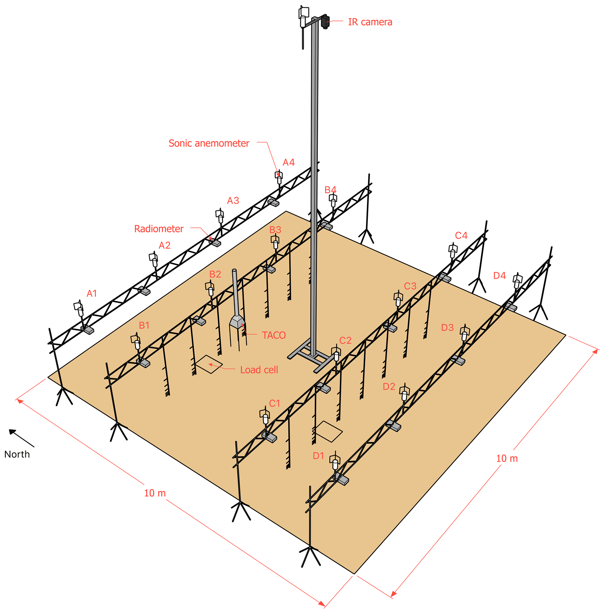
Figure 1 Sketch of the burn plot and the instruments deployed to the plot. The four capital letters (A, B, C and D) denote the four trusses, and the four numbers (1, 2, 3, 4) refer to the 3D sonic anemometers on the trusses. Posts hanging on trusses B and C show the heights and location of thermocouples. The center post indicates the position of the infrared camera. The boxes next to the sonic anemometers indicate the radiometer–spectral camera pairs. The rectangular box on the ground indicates fuel cells for fuel loading estimation. The symbol near B2 indicates the TACO for emission data collection.

2 Method

2.1 Experiment and instrumentation

The experimental burn that this study focuses on occurred on 20 May 2019 in a pitch and loblolly pine plantation at the Silas Little Experimental Forest in New Lisbon, New Jersey. This particular burn was part of a broader series of 35 densely instrumented, low-intensity surface fire experiments on 100 m² (10 m × 10 m) plots in this plantation conducted between March 2018 and June 2019 by a research project funded by the Department of Defense's Strategic Environmental Research and Development Program (SERDP). The overall goal of this research project was to collect data using laboratory-scale (10⁰–10¹ m²) experiments, intermediate or fuel-bed-scale (10² m²) burns, and management-scale (10^3–4 m²) prescribed fires to improve the understanding of combustion processes and fire–atmosphere interactions across scales (Gallagher et al., 2022; Skowronski, 2021).

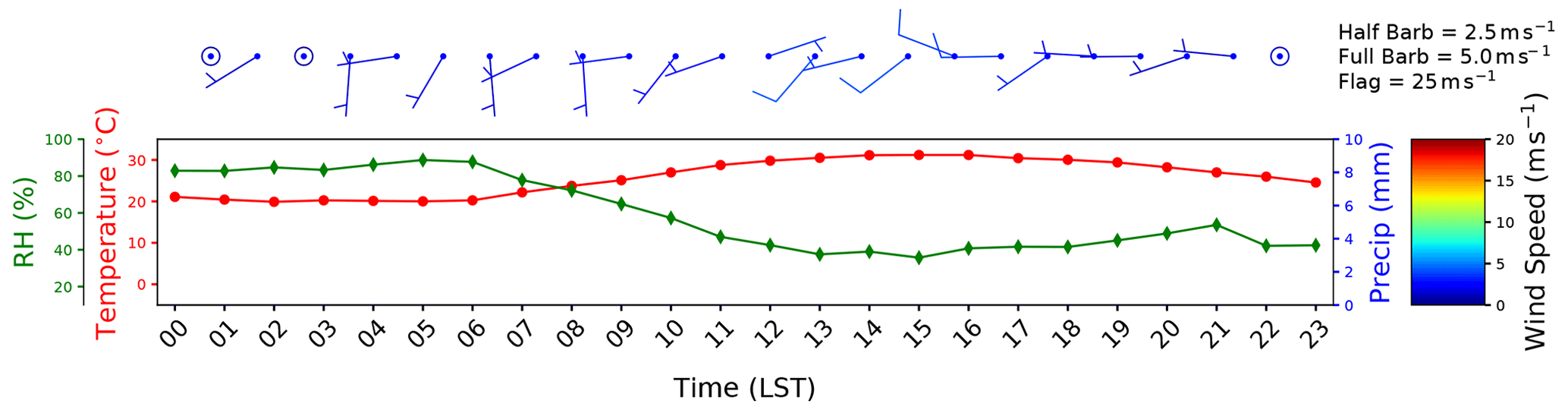
Figure 2 Surface meteorological condition on 20 May 2019, the day of the experimental burn, observed by the weather station approximately 200 m northeast of the burn plot.

As shown in Fig. 1, the 100 m² burn plot was densely monitored by instruments mounted on four parallel east–west-oriented trusses (A–D). On each truss, four 3D fast-response sonic anemometers (R.M. Young 81000V, Traverse City, MI, USA) were mounted at 2.5 m above ground level (a.g.l.) to collect the east–west (u), north–south (v), and vertical (w) velocity components and temperature at a sampling rate of 10 Hz (Clark et al., 2022a). Additional 10 Hz temperature data were also obtained using fine-wire thermocouples (Omega SSRTC-GG-K-36, Omega Engineering, Inc., Stamford, CT, USA) mounted at a range of heights (0, 5, 10, 20, 30, 50, 100 cm) below the two inner trusses (B and C) (Clark et al., 2022b). A radiometer–visible spectrum camera pair was mounted adjacent to each sonic anemometer to measure radiative heat fluxes and flame arrival times and persistence (Kremens et al., 2022). Spatially explicit fire spread data were derived from infrared data collected by an infrared video camera (A655SC, FOL6 100.0-650.0 C lens, FLIR Systems Inc., Wilsonville, OR, USA) mounted on top of a 10 m tower in the center of the plot (Skowronski et al., 2022a). A custom field calorimetry hood (labeled TACO next to B2) with an inlet oriented over a portion of the fuel bed was used to sample O₂, CO₂ and CO concentrations in buoyant plumes (Campbell-Lochrie et al., 2021, 2022). Gas concentrations were measured at 1 Hz using an infrared gas analyzer (Crestline NDIR 7911, Crestline, Livermore, CA, USA).

The analyses here focused only on the data from the 4 × 4 sonic anemometer array. All sonic anemometer data underwent a quality assurance and control process to remove spurious values (Clark et al., 2022a). Initially, data that were collected prior to a designated common start time were removed, providing a starting point for the observations for the burn period. Next, the data from sonic anemometers include a self-reporting diagnostic column where any non-zero number is considered an invalid measurement, so any measurement that reported a non-zero diagnostic code was removed. Following these initial steps, data that fell outside the sonic anemometer operating parameters (wind speed: ± 40 m s⁻¹; temperature: ± 50 ^∘C) were also removed.

The horizontal wind velocities were rotated into a streamwise coordinate system where the u component (streamwise component) is aligned with the prevailing wind direction, and the v component (cross-stream component) is perpendicular to the prevailing wind direction pointing to the left. Vertical winds were not corrected for tilt because of the short (< 30 min) observational period and because the burn plot was on level ground, and each sonic anemometer was carefully mounted and leveled so that the wind sensors were very close to true horizontal and vertical planes. The results (presented below) indeed suggested that the contamination of vertical velocity by horizontal velocities was negligibly small as the average vertical wind component during the pre-burn period was nearly zero.

2.2 Fuel and ambient atmospheric conditions

The primary fuel for this burn was pitch pine needles (Pinus rigida Mill.). Based on biometric and terrestrial laser scan measurements collected pre- and post-burn, the fuel mass was estimated to be about 0.5 kg m⁻² and fuel moisture content about 5.5 % (Skowronski et al., 2022b).

The ambient atmospheric conditions on the day of the burn are indicated using the data from a surface weather station located approximately 200 m northeast of the burn plot that has a similar type of land cover to the burn plot (Fig. 2). Ambient winds were very weak in the morning, varying in direction between south and west. Wind speeds increased in midday to about 5 m s⁻¹, along with a direction shift to southwest and west. This wind speed increase was likely due to the mixing of higher winds from above to the surface as the mixing layer grew higher during the day. The growth of the mixing layer was a result of increased turbulent mixing associated with surface heating, as indicated by an increase in surface temperatures from about 20 ^∘C in the morning to slightly above 30 ^∘C around 14:00 local standard time (LST) and a corresponding decrease in relative humidity from over 80 % in the morning to less than 40 % in the early afternoon.

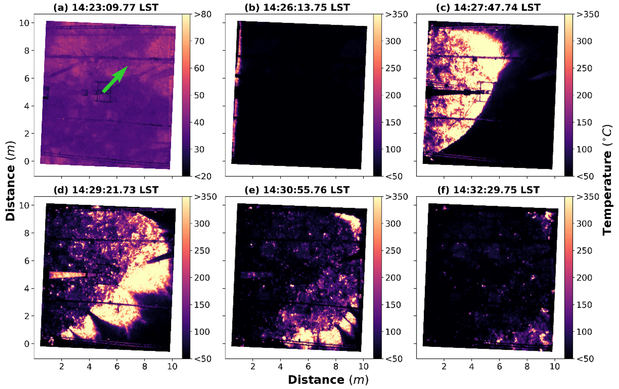
Figure 3 Infrared images taken at 10 m above the center of the burn plot showing fuel bed temperature before (a), near (b) and after (c–f) ignition. The green arrow indicates the direction of background wind.

2.3 Fire spread

The experiment started around 14:25 LST when a single 10 m cotton cord was soaked in accelerant, ignited and then dropped on the fuel bed to produce a single, near-linear ignition across the western border of the plot. Infrared imagery data (Fig. 3) captured by the overhead infrared camera are used to evaluate the changes in temperature from just before ignition (Fig. 3a), immediately after ignition (Fig. 3b) and through the period following the ignition, as the line fire spread with winds across the plot (Fig. 3c–f). The average fire spread rate throughout the burn was estimated from these data to be approximately 5.4 cm s⁻¹. The ignition produced a line fire parallel to the western boundary of the plot (Fig. 3b). The line fire spread in the direction of the west-southwesterly background wind towards the east-northeast over the next few minutes (Fig. 3c and d). The initial spread was faster on the northern portion of the domain, as expected from the south-southwesterly wind direction. As the fire burned through the northern portion of the plot, the fire front caught up in the southern portion (Fig. 3e). The fire ended at around 14:32:16 LST as the fire front reached the eastern boundary of the plot and ran out of fuel to continue (Fig. 3f).

2.4 Data analysis

The quality-controlled 10 Hz wind and temperature data from the 3D sonic anemometers are used to calculate turbulent perturbations, defined as the differences between the instantaneous observations and the mean values:

$$\begin{array}{}\text{(1)}& {\mathit{\phi }}^{\prime }=\mathit{\phi }-\stackrel{\mathrm{‾}}{\mathit{\phi }},\end{array}$$

where $\stackrel{\mathrm{‾}}{\mathit{\phi }}$ is the mean value that is estimated by block averages:

$$\begin{array}{}\text{(2)}& \stackrel{\mathrm{‾}}{\mathit{\phi }}={\sum }_{n=\mathrm{1}}^N{\mathit{\phi }}_n.\end{array}$$

Here, N is the number of samples over the averaging period or the time block, and the mean values represent the mean state of the atmospheric flow. In traditional turbulence studies, mean state is usually determined by averaging the data over a period of a few minutes up to 1 h, depending on atmospheric stability and the scale of interest. However, the block-averaged values during the period of active burning are likely to be contaminated by the fire and therefore poorly represent the mean background flow. To resolve this issue, Seto et al. (2013) and Heilman et al. (2015) proposed that the block-averaged means for the fire period be replaced by block-averaged means calculated during the pre-burn period. In order to adopt this approach, the observational period is divided into three periods representing pre-burn, burn and post-burn, which are described in detail below.

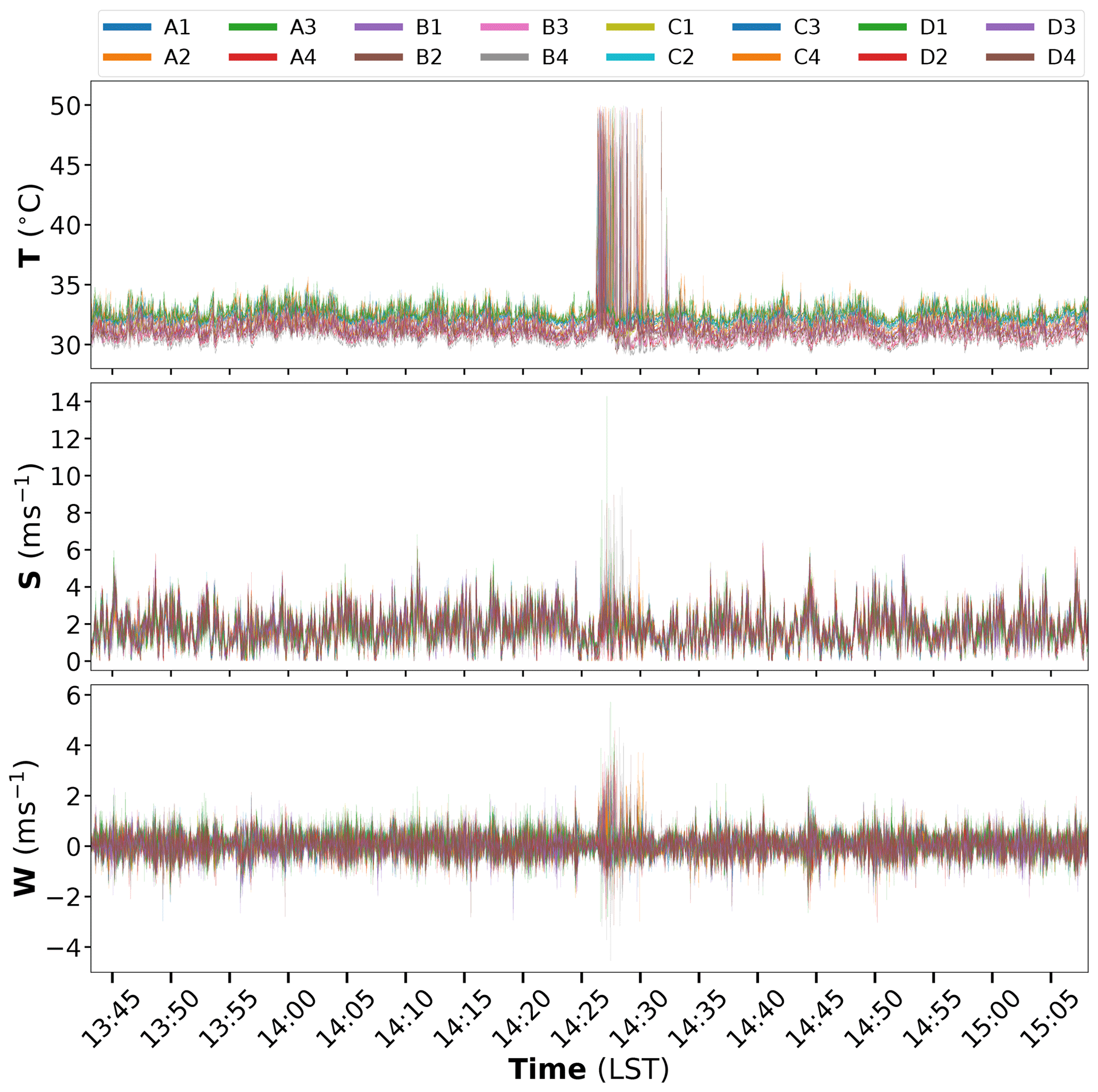
Figure 4 Time series of 10 Hz observations of temperature (T), horizontal wind speed (S) and vertical wind component (w) observed by the 16 sonic anemometers.

The arrival of the fire front at most locations in the sonic anemometer array was clearly marked by a sharp rise in temperature (Fig. 4). However, the magnitudes of the temperature increase, and the rates of increase vary with the location of the sonic anemometers because the shape of the flame front was irregular (Fig. 3). Note that the sonic temperatures are limited to 50 ^∘C, which is the operational range for the instruments beyond which data are deemed unreliable. Based on the temperature time series and the time when the fire was ignited along the western boundary (14:25 LST), the 10 min period from 14:15:13 through 14:25:12 LST is defined as the pre-burn period over which the mean values for u, v, S (horizontal wind speed), w and T are calculated, and these values are used for computing perturbations for the entire experiment. The definition of the burn period, however, is complicated by the fact that the fire front reaches/leaves each sonic anemometer at a different time, and consequently the true burn period across the plot varies somewhat depending on the location of each sonic anemometer.

To create a robust definition of the burn period that can be applied to all the sonic anemometers in the 4 × 4 array, and eventually to other burns in the broader burn series, the sharp rise in sonic temperatures associated with the fire front is measured using integer (n) multiples of the standard deviation (denoted using σ) of the average temperature over the pre-burn period. A threshold value that is too small (e.g., 1 or 2 times standard deviation) may not distinguish the increase in temperature associated with the fire front from normal temperature fluctuations during the day, but a value that is too large (e.g., 10 time standard deviation) may fail to detect the fire front associated with a small or moderate temperature increase. Figure 5 shows the number of sonic anemometers whose temperatures exceed n × σ as n increases from 1 to 35 and the length of the exceedance period. As n increases from 1 to 8 or the threshold value for fire-induced temperature increase changes from 1σ to 8σ, the number of sonic anemometers drops from 16 to 13, and the period drops sharply from just under 60 min to about 6 min. Continued increases in the threshold values from 8σ to 25σ result in no change in the number of anemometers and very little change in the length of the period (less than 1 min). This analysis suggests that 8σ could be used as the threshold for temperature increases associated with the fire front. Thresholds lower than 8σ would imply a burn period of 30 to 60 min long that, according to the time series in Fig. 4, would include periods of no fire and therefore de-emphasize the effects of the fire in the resulting analyses. Applying this criterion to all the sonic anemometers and defining the burn period as between the first and last sonic temperature at or above the threshold leads to the selection of the burn period as 14:26:13 to 14:32:29 LST. Finally, the 10 min following the burn period (14:32:30 to 14:42:29 LST) is defined as the post-burn period.

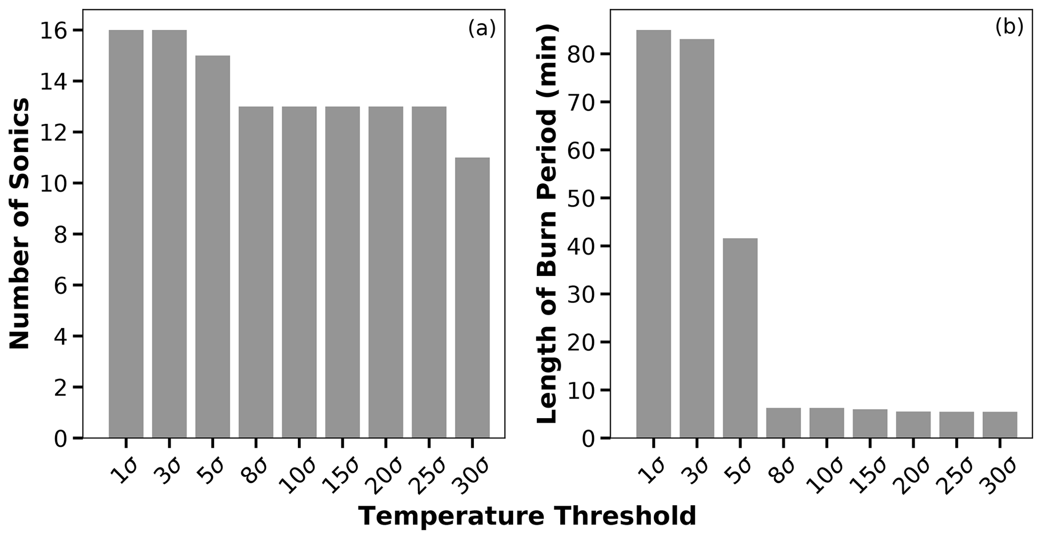
Figure 5 The number of sonic anemometers that recorded temperatures at or above a given threshold value (a) and the length of period over which the threshold was reached or exceeded (b). The symbol σ denotes pre-burn period temperature standard deviation.

Following the establishment of the three periods, wind and temperature perturbations are calculated using Eqs. (1) and (2), where the pre-burn averaged values are used as means for the burn and post-burn periods. Strictly speaking, the perturbations calculated for the burn and post-burn periods are not classical turbulent perturbations; to differentiate the features from classical turbulence, they should be interpreted as being primarily fire-induced turbulent perturbations.

As noted above, horizontal wind velocity is rotated into a streamwise coordinate where the x component (streamwise component, u) is aligned with the prevailing wind direction, and the y component (cross-stream component, v) is perpendicular and pointing to the left of the prevailing wind. The prevailing wind direction for the rotation is determined by the 10 min pre-burn period average of wind directions across all 16 sonic anemometers. The average wind directions during the pre-burn period vary slightly across the 16 sonic anemometers, with mean and median wind directions of 225 and 226^∘ respectively. The subtle variations in wind directions are possibly due to slight error in sensor alignment, rather than actual flow heterogeneity. The 226^∘ is used as the prevailing wind direction for the purpose of coordinate rotation.

The quality-controlled, coordinate-rotated data from the sonic anemometers are analyzed to determine fire-induced changes to turbulence intensity, vertical heat fluxes, and vertical fluxes of horizontal momentum also known as shear stress just above the combustion zone by comparing values between the pre-burn and the burn periods. The values are also compared between the pre-burn and post-burn periods to determine how quickly the effects of fire dissipate or how fast the atmosphere returns to the ambient state.

Turbulence intensity is measured by the turbulent kinetic energy (TKE), defined as the sum of the variance of the three velocity components:

$$\begin{array}{}\text{(3)}& \mathrm{TKE}=\left(\stackrel{\mathrm{‾}}{u^{\prime \mathrm{2}}}+\stackrel{\mathrm{‾}}{v^{\prime \mathrm{2}}}+\stackrel{\mathrm{‾}}{w^{\prime \mathrm{2}}}\right)/\mathrm{2}.\end{array}$$

Turbulent shear stress is commonly measured by shear velocity or friction velocity denoted by u_∗, and the square of friction velocity is related to the magnitude of the kinematic vertical flux of horizontal momentum:

$$\begin{array}{}\text{(4)}& u_{\ast }^{\mathrm{2}}={\left({\stackrel{\mathrm{‾}}{u^{\prime }{w}^{\prime }}}^{\mathrm{2}}+{\stackrel{\mathrm{‾}}{v^{\prime }{w}^{\prime }}}^{\mathrm{2}}\right)}^{\frac{\mathrm{1}}{\mathrm{2}}},\end{array}$$

where $u^{\prime }{w}^{\prime }$ and $v^{\prime }{w}^{\prime }$ are the vertical fluxes of streamwise and cross-stream momentum flux, respectively, and the overbar denotes time average. The average period is 1 min for this analysis to be consistent with previous studies on fire-induced turbulence (Seto et al., 2013; Heilman et al. 2021). Vertical kinematic heat flux is calculated as $\stackrel{\mathrm{‾}}{T^{\prime }{w}^{\prime }}$, and the averaging period is also 1 min.

For the analyses of vertical turbulent fluxes of heat and horizontal momentum, a quadrant analysis technique (Katul et al., 1997, 2006; Heilman et al., 2021) is utilized to delineate the contributions to the turbulent heat or momentum transfer from four types of processes corresponding to the four quadrants of a w^′ (horizontal) and φ^′ (vertical) coordinate, where the w^′ denotes vertical velocity perturbation, and φ^′ denotes perturbations of temperature (T^′) or horizontal wind speed (S^′) in heat or momentum flux calculations, respectively. The four quadrants are Q1 – ${\mathit{\phi }}^{\prime }{w}^{\prime }$ > 0, ${\mathit{\phi }}^{\prime }>\mathrm{0}$, $w^{\prime }>\mathrm{0}$, Q2 – ${\mathit{\phi }}^{\prime }{w}^{\prime }$ < 0, ${\mathit{\phi }}^{\prime }>\mathrm{0}$, $w^{\prime }<\mathrm{0}$, Q3 – ${\mathit{\phi }}^{\prime }{w}^{\prime }$ > 0, ${\mathit{\phi }}^{\prime }<\mathrm{0}$, $w^{\prime }<\mathrm{0}$ and Q4 – ${\mathit{\phi }}^{\prime }{w}^{\prime }$ < 0, ${\mathit{\phi }}^{\prime }<\mathrm{0}$, $w^{\prime }>\mathrm{0}$. Note that the perturbation in horizontal wind speed (S^′), rather than the streamwise or cross-wind components (u^′ or v^′), is used for computing momentum flux, following Heilman et al. (2021):

$$\begin{array}{}\text{(5)}& {\displaystyle }{S}^{\prime }=S-\stackrel{\mathrm{‾}}{S}\text{(6)}& {\displaystyle }S=\sqrt{u^{\mathrm{2}}+v^{\mathrm{2}}}.\end{array}$$

Table 1 Vertical turbulent transfer events and the associated quadrat designations.

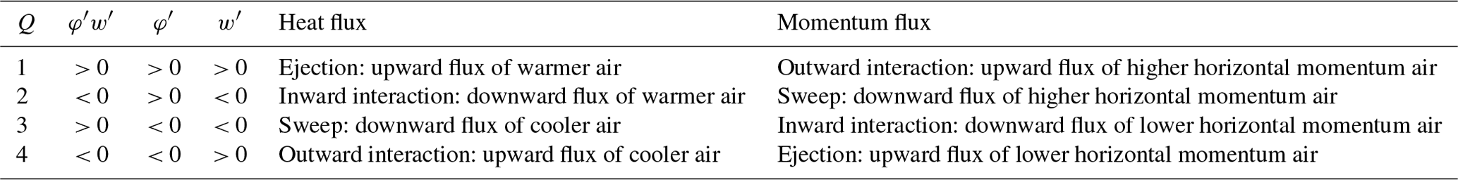
The quadrant analysis is also known as sweep–ejection analysis (Heilman et al., 2021), which associates each quadrant with a specific type of vertical turbulent transfer events. The names of the events and the associated quadrant designations, which are different for turbulent heat and momentum fluxes, are given in Table 1.

Based on the definition in Table 1, ejection (Q1) and sweep (Q3) events contribute to positive vertical turbulent heat flux through the upward transfer of warmer air from below (ejection) or the downward transfer of cooler air from above (sweep), while inward interaction (Q2) and outward interaction (Q4) events contribute to negative turbulent heat flux through the downward transfer of warmer air from above (inward interaction) or the upward transfer of cooler air from below (outward interaction). For vertical flux of horizontal momentum, inward interaction and outward interaction events contribute to positive flux through the upward transfer of faster moving air (outward interaction) or the downward transfer of slower moving air (inward interaction), while sweep and ejection events contribute to negative momentum flux through the downward transfer of faster moving air (sweep) or the upward transfer of slower moving air (ejection). Note that the warmer/cooler or faster/slower air is relative to the air in the adjacent layers.

The sweep–ejection analysis calculates the proportion of a given type of events by simply counting the number of events or the data points in the 10 Hz time series that fall within the given quadrant. The contributions of the given type of events to the average turbulent fluxes over a given time period (T_p) are calculated, following Heilman et al. (2021), by the integral

$$\begin{array}{}\text{(7)}& {\stackrel{\mathrm{‾}}{{\mathit{\phi }}^{\prime }{w}^{\prime }}}_Q={\displaystyle \frac{\mathrm{1}}{T_{\mathrm{p}}}}\underset{\mathrm{0}}{\overset{T_{\mathrm{p}}}{\int }}{\mathit{\phi }}^{\prime }\left(\mathit{\tau }\right)w^{\prime }\left(\mathit{\tau }\right){\mathit{\epsilon }}_Q\mathrm{d}\mathit{\tau },\end{array}$$

where ε_Q is 1 for the given quadrant and zero otherwise, τ is time, and φ^′ is temperature or horizontal wind speed perturbation for heat or momentum fluxes, respectively.

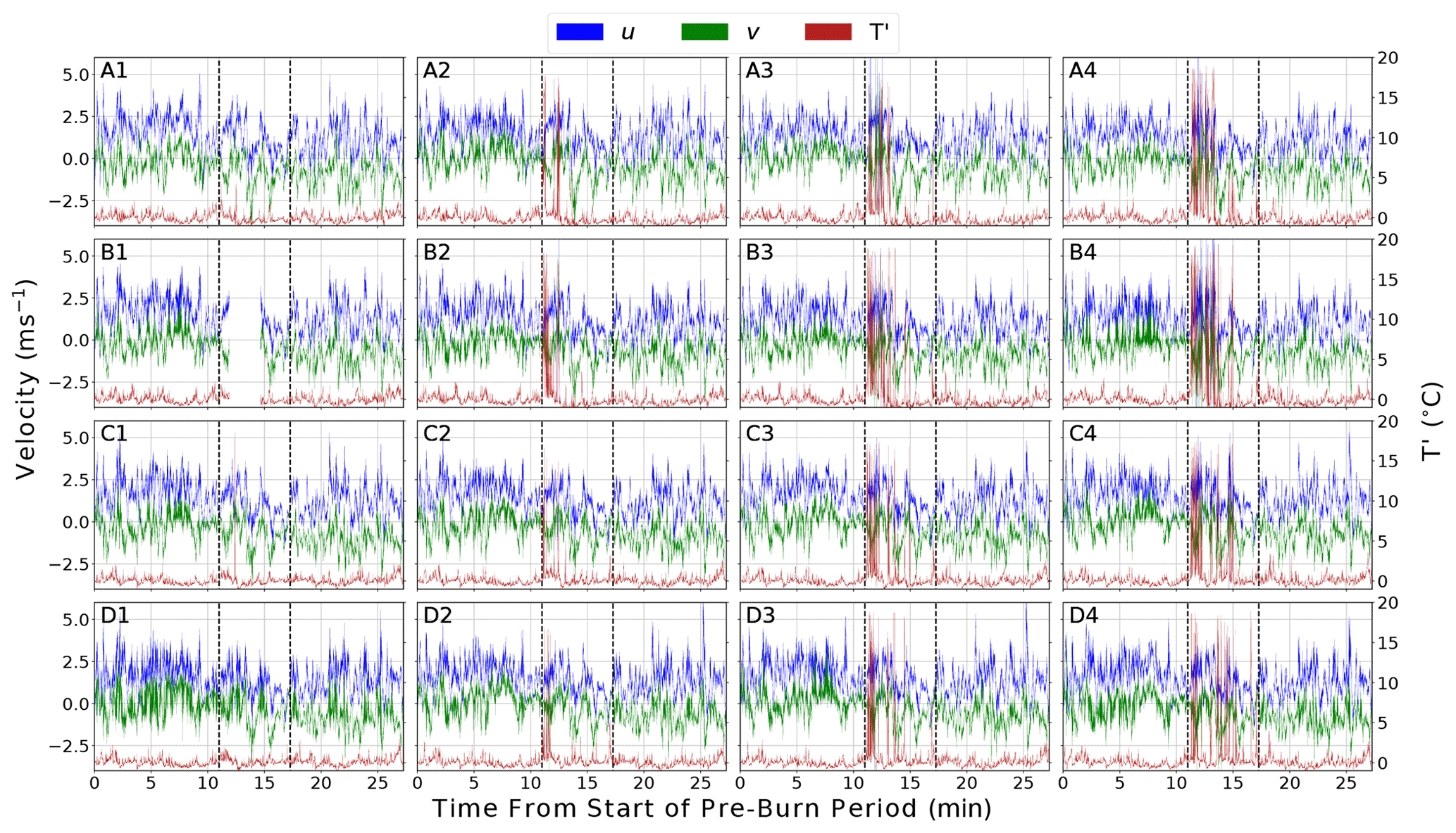
Figure 6 Time series of 10 Hz streamwise (u; blue) and cross-stream (v; green) wind velocity components and temperature perturbations (T^′; red) recorded by each sonic anemometer at 2.5 m above the ground. The vertical dashed black lines indicate the burn period determined by the first and last occurrence of $T^{\prime }\ge \mathrm{8}\mathit{\sigma }$. Time is the minutes since the start of the pre-burn period.

3 Results and discussion

3.1 Fire-induced perturbations to wind and temperature

Before we examine fire-induced changes to turbulence in the ambient atmosphere, we first take a look at the response of the instantaneous temperature and wind to the surface line fire recorded by the 16 sonic anemometers as the fire spread from west to east across the 10 m × 10 m burn plot (Fig. 6). Note that perturbation temperatures (T^′; see Eq. 1), instead of actual temperatures, are shown to accommodate the magnitude difference between temperature and wind, facilitating a more coherent visualization of the joint effects of the fire on temperature and wind.

The natural or non-fire fluctuation recorded during the pre-burn period is small, with magnitudes generally less than 2.5 m s⁻¹ for u, 1 m s⁻¹ for v and 2.5 ^∘C for T^′. The fire impinging upon the sonic anemometers is marked by a sharp increase in T^′, but the magnitude of the temperature changes depends heavily on location, from very little change on the western side (A1, B1, C1, D1) of the burn plot, where the fire was ignited, to a nearly 20 ^∘C increase on the eastern side (A4, B4, C4, D4). This spatial heterogeneity in T^′ is consistent with the pattern of the fire spread from the western boundary toward the east and northeast by the southwesterly ambient wind (Fig. 4). During the burn period, the u fluctuations decreased slightly, while the v fluctuations increased. The v component no longer fluctuated around zero, as in the pre-burn period, but rather it was dominated by negative values, indicating a systematic shift in wind direction. There was a tendency for u and T^′ to return towards the pre-burn conditions after the burn, but the v component remained negative during the post-burn period.

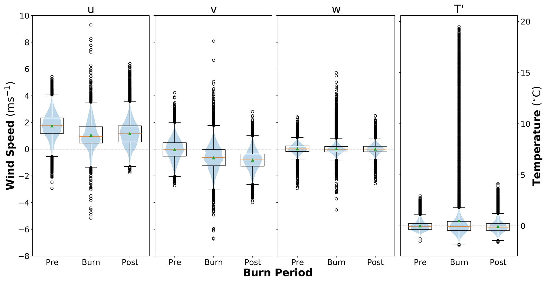
Figure 7 Distributions of 10 Hz streamwise (u), cross-stream (v) and vertical (w) wind velocity components and temperature perturbations (T^′) from all 16 sonic anemometers during pre-burn, burn and post-burn periods. The box represents the 25th and 75th percentile of the data, with data inside the whiskers representing 99.3 % of the data. The orange line in the boxes is the median value, the green triangle is the mean and the blue shading is the density of values of the data.

The observed changes in the distribution of wind and temperature values associated with the fire at all 16 sonics are summarized by the box-and-whisker plots in Fig. 7. The pre-burn mean is 1.7 m s⁻¹ for the streamwise wind component u and near zero (−0.04 m s⁻¹) for the cross-stream component v. The pre-burn vertical velocity distribution also has a near-zero mean, which confirms that the sonic anemometers were well-leveled. During the burn period, the mean of u dropped in magnitude from 1.7 to 1.05 m s⁻¹, while the mean of v increased in magnitude from −0.04 to −0.65 m s⁻¹, indicating an overall shift in wind direction from southwesterly to west-southwesterly. This change in the horizontal wind components suggests that ambient air was drawn towards the fire, producing convergence at the fire front. There is also a fire-induced widening of the distributions of the horizontal wind components, particularly the v component, and an increase in the number of outliers with magnitudes that nearly doubled the pre-fire magnitude. The large negative values in v during the burn period reinforce the suggestion of convergence in the vicinity of the fire.

Interestingly, there is little evident change in the overall distribution of w during the burn period, except that more and larger outliers are indicated. The maximum updrafts (downdrafts) during the burn period reach speeds of nearly 6 m s⁻¹ (−5 m s⁻¹), which is more than double those of the pre- and post-burn periods, suggesting that intermittent turbulent eddies associated with the fire could have a strong impact on vertical velocity just above the fuel bed. The T^′ distribution also widens substantially during the burn period (σ = 4.24 ^∘C) compared to the pre-burn period (σ = 0.48 ^∘C), with the maximum temperature perturbation reaching nearly 20 ^∘C.

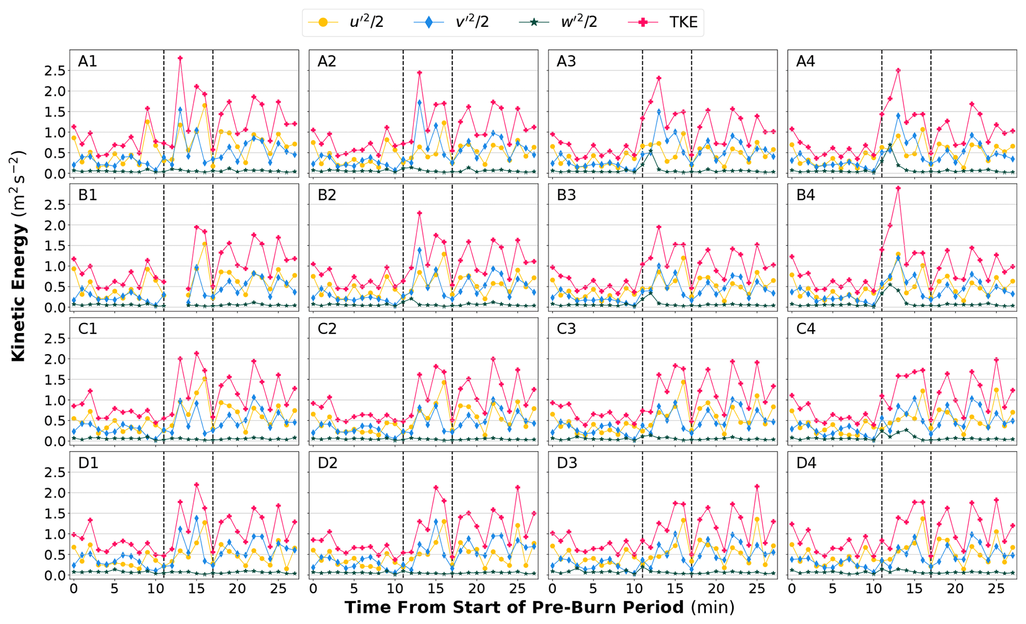
Figure 8 Time series of 1 min averaged turbulent kinetic energy (TKE) (red) for each sonic anemometer and the three components of velocity variance, $u^{\prime \mathrm{2}}/\mathrm{2}$ (yellow), $v^{\prime \mathrm{2}}/\mathrm{2}$ (blue) and $w^{\prime \mathrm{2}}/\mathrm{2}$ (green) that make up the TKE. The vertical dashed black lines indicate the burn period determined by the first and last occurrence of $T^{\prime }\ge \mathrm{8}\mathit{\sigma }$. Time is the minutes since the start of the pre-burn period.

The influence of the fire on the horizontal wind components continues into the post-burn period, as the post-burn distributions of u and v fall between those of the pre-burn and burn periods. In contrast, the post-burn w distribution returns to a distribution very close to that of the pre-burn period. Similarly, the T^′ distribution during the post-burn period is very similar to that of the pre-burn period. The similarities between the w^′ and T^′ distributions suggest that the two variables are closely related to each other, with large updrafts during the burn period being generated primarily by heating. This result suggests that the fire-induced circulation exhibits behavior more consistent with a buoyant plume than mechanically forced rising motion resulting from converging surface air.

3.2 Intensity of fire-induced turbulence

We now explore the modifications of the fire to atmospheric turbulence properties just above the combustion zone. The first question to address is how turbulence intensity quantified by TKE in Eq. (3) is modified by the fire and how the modification may vary with location in the burn plot. Figure 8 shows time series of 1 min averaged TKE and its three components (the variance of the three velocity components) for each of the sonic anemometers. The time series indicate lower TKE values in the pre-burn period, larger values during the burn period and values remaining high in the post-burn period. The burn period TKE is primarily driven by an increase in horizontal velocity variance, $\stackrel{\mathrm{‾}}{u^{\prime \mathrm{2}}}$ and $\stackrel{\mathrm{‾}}{v^{\prime \mathrm{2}}}$, particularly the cross-stream component $\stackrel{\mathrm{‾}}{v^{\prime \mathrm{2}}}$. The TKE values remain high into the post-burn period, and, at several sonic anemometers (D3 and C4), the post-burn TKE peaks are comparable with or higher than the peaks observed during the burn period.

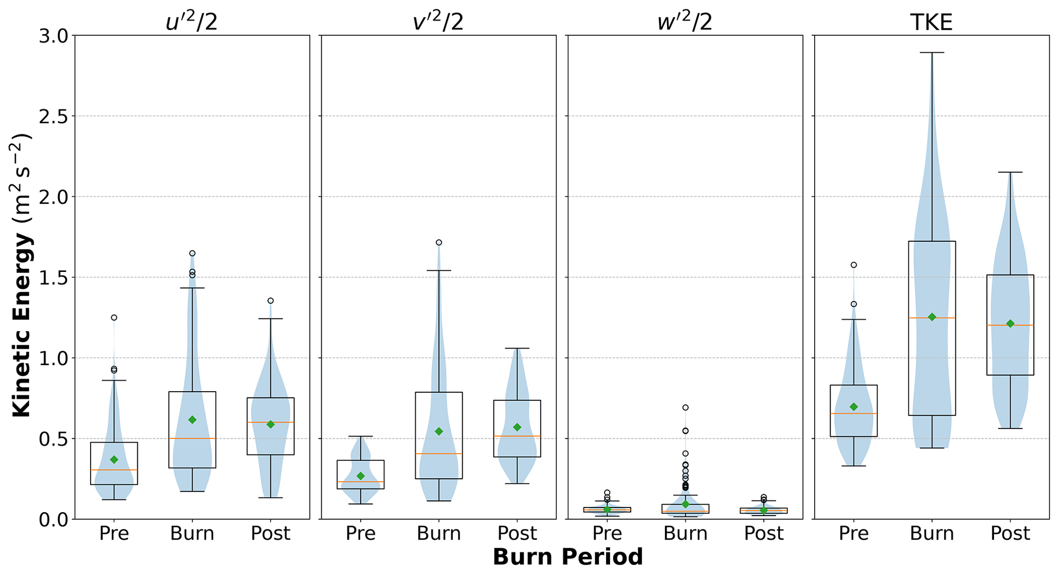
Figure 9 Distributions of turbulent kinetic energy (TKE) and the three components of velocity variance ($u^{\prime \mathrm{2}}/\mathrm{2}$, $v^{\prime \mathrm{2}}/\mathrm{2}$ and $w^{\prime \mathrm{2}}/\mathrm{2}$) that make up the TKE from all 16 sonic anemometers during the pre-burn, burn and post-burn periods. The box represents the 25th and 75th percentile of the data, with data inside the whiskers representing 99.3 % of the data. The orange line in the boxes is the median value, the green diamond is the mean and the blue shading is the density of values of the data.

The box-and-whisker plots in Fig. 9 depict the fire-induced changes to the distribution of turbulence intensity as observed by all 16 sonic anemometers. Averaging across all the instruments, the burn period mean TKE is 1.25 m² s⁻², which is roughly double the pre-burn mean of 0.697 m² s⁻². The interquartile range of the burn period TKE is nearly 3 times the pre-burn period range. Despite the increase in the mean and the interquartile range of the TKE from the pre-burn to the burn period, the mean TKE values are still below 3 m² s⁻², which is a threshold sometimes used as an indicator for substantial boundary-layer turbulence (Stull, 1988; Heilman and Bian, 2013), suggesting that this low-intensity surface line fire fails to produce a substantially turbulent environment at the levels just above the fuel bed. The mean TKE in the post-burn period does not return to that of the pre-burn period and remains elevated (1.21 m² s⁻²). While the $\stackrel{\mathrm{‾}}{w^{\prime \mathrm{2}}}$ returns to the pre-burn conditions, the horizontal components remain elevated.

More specifically, $\stackrel{\mathrm{‾}}{u^{\prime \mathrm{2}}}$ and $\stackrel{\mathrm{‾}}{v^{\prime \mathrm{2}}}$ make up 53.0 % and 38.5 % of the average pre-burn TKE, respectively. During the burn period, the contribution to TKE from $\stackrel{\mathrm{‾}}{u^{\prime \mathrm{2}}}$ decreases slightly to 49.1 %, and the contribution from $\stackrel{\mathrm{‾}}{v^{\prime \mathrm{2}}}$ increases substantially to 43.3 %. As noted earlier (Figs. 6 and 7), the burn period also exhibits a larger range of horizontal and vertical wind components, which is consistent with the larger range of TKE values in Fig. 9.

In the post-burn period, the distribution of vertical velocity variance returns to the pre-burn distribution. However, the range of values in the horizontal components is smaller during the post-burn period than the burn period but still larger than during the pre-burn period. The medians of the horizontal TKE components are higher in the post-burn period than in either of the other periods. While the $\stackrel{\mathrm{‾}}{u^{\prime \mathrm{2}}}$ outliers (above the 99.3rd percentile) decrease, the $\stackrel{\mathrm{‾}}{v^{\prime \mathrm{2}}}$ outliers increase in magnitude. As was previously discussed, post-burn average wind directions differ slightly from the pre-burn, accompanied by increases in the magnitude of the horizontal winds (Figs. 6 and 7). This result is consistent with elevated TKE values persisting into the period after the end of the fire.

Additional analysis of the variance of the three velocity components enables an assessment of turbulence anisotropy indicated by the ratio of $\stackrel{\mathrm{‾}}{w^{\prime \mathrm{2}}}$ to 2 × TKE. When this ratio approaches $\mathrm{1}/\mathrm{3}$ for a given time period, the period can be said to experience an isotropic turbulent regime (Heilman et al., 2015). The mean $\stackrel{\mathrm{‾}}{w^{\prime \mathrm{2}}}$ for all the sonic anemometers is 0.0597 m² s⁻² for the pre-burn period, 0.0931 m² s⁻² for the burn period and 0.052 m² s⁻² for the post-burn period, which yields an anisotropy ratio of 0.042, 0.036 and 0.021 for the pre-burn, burn and post-burn periods, respectively. As the anisotropy ratios are well below $\mathrm{1}/\mathrm{3}$ in all three periods, the turbulence regime just above the combustion zone remains anisotropic at all time. It is worth noting that in contrary to the belief that the increase in vertical velocity variance in response to the surface heating during the burn should act to move turbulence towards a more isotropic regime, the ratio here is slightly smaller during the burn period than the pre-burn period, largely because the fire-induced increase in the cross-stream velocity variance is larger than the increase in the vertical velocity variance. Heilman et al. (2015) calculated the anisotropy ratios at 3 m above ground (a.g.) for two forest understory fires. The ratio decreased from 0.118 to 0.0718 from pre-burn to burn in one experiment but increased from 0.089 pre-burn to 0.13 in another experiment. Since the sonic anemometers located on the western and southern sides of the burn plot show no clear increase in $\stackrel{\mathrm{‾}}{w^{\prime \mathrm{2}}}$, the anisotropy ratio is also calculated for each sonic to verify that the mean values did not mask anisotropy variations at individual locations in the burn plot. No individual sonic anemometer reaches a ratio of $\mathrm{1}/\mathrm{3}$, and the highest individual ratio (0.133) is found at sonic anemometer A4 during the burn period. This result indicates that overall, the TKE just above the combustion zone is highly anisotropic and is dominated by the horizontal components for this burn. This result is not surprising as the sonic anemometers are located only 2.5 $\mathrm{m}\mathrm{a}.\mathrm{g}.$ where horizontal turbulence would be expected to dominate over vertical turbulence (Heilman et al., 2015).

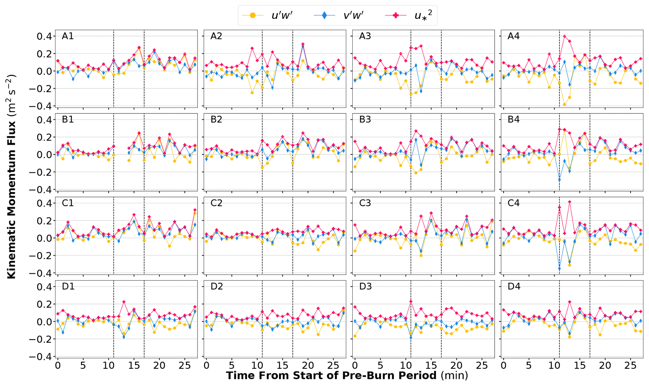
Figure 10 Time series of 1 min averaged friction velocity squared ($u_{\ast }^{\mathrm{2}}$, pink pluses) and its two components, the streamwise kinematic momentum flux, $\stackrel{\mathrm{‾}}{u^{\prime }{w}^{\prime }}$ (yellow circle), and the cross-stream kinematic momentum flux, $\stackrel{\mathrm{‾}}{v^{\prime }{w}^{\prime }}$ (blue diamonds), for each of the 16 sonic anemometers. The vertical dashed black lines indicate the burn period determined by the first and last occurrence of $T^{\prime }\ge$ 8σ. Time is the minutes since the start of the pre-burn period.

3.3 Fire-induced shear stress

To address the question on how surface fires alter turbulent momentum transfer between the combustion zone and the atmosphere above, we next explore fire-induced changes to turbulent momentum fluxes or shear stress measured by friction velocity described in Eq. (4). Figure 10 shows time series of 1 min averaged $u_{\ast }^{\mathrm{2}}$ and the streamwise $\stackrel{\mathrm{‾}}{u^{\prime }{w}^{\prime }}$ and cross-stream $\stackrel{\mathrm{‾}}{v^{\prime }{w}^{\prime }}$ stress components (the momentum flux), measured by each of the sonic anemometers for the three periods. Kinematic momentum fluxes and $u_{\ast }^{\mathrm{2}}$ are similar across all the sonic anemometers during the pre-burn period, although three of the northernmost instruments (A2, A3 and A4) indicate a negative spike in $\stackrel{\mathrm{‾}}{u^{\prime }{w}^{\prime }}$ just before the start of the burn period. These spikes contribute to an increase in $u_{\ast }^{\mathrm{2}}$ during this time as well. It is unclear what caused these features, but candidates include an anomalous burst of wind along the northern edge of the burn plot and possible contamination of the wind data by activities of the burn managers as they prepared to ignite the fire.

During the burn period, the values of $\stackrel{\mathrm{‾}}{u^{\prime }{w}^{\prime }}$ and $\stackrel{\mathrm{‾}}{v^{\prime }{w}^{\prime }}$ increase somewhat, leading to increases in the $u_{\ast }^{\mathrm{2}}$ values. The fire-induced changes generally increase in magnitude from west (left) to east (right) and south to north, consistent with the fire-spread pattern. The largest increase occurs at the easternmost (right) locations, particularly A4 and C4, where $u_{\ast }^{\mathrm{2}}$ values nearly doubled. The smallest increases are not found at the westernmost locations but at C2 and D2. With a few exceptions, $\stackrel{\mathrm{‾}}{u^{\prime }{w}^{\prime }}$ and $\stackrel{\mathrm{‾}}{v^{\prime }{w}^{\prime }}$ are negative in the beginning of the burn period, turning positive later in the period. The $\stackrel{\mathrm{‾}}{u^{\prime }{w}^{\prime }}$ values exhibit the largest burn period variation at A4, followed by B4, and similar patterns are observed for $\stackrel{\mathrm{‾}}{v^{\prime }{w}^{\prime }}$. Overall, variations in $u_{\ast }^{\mathrm{2}}$ suggest an increase in shear stress magnitude in the burn period compared to the pre-burn period, with the easternmost sonic anemometers recording 1 min averaged values that are far greater than the westernmost sonic anemometers.

During the post-burn period, some sonic anemometers (A2, B2, C1, C2, D2) recorded higher $u_{\ast }^{\mathrm{2}}$ than during the burn period, while others (A1, B1, B3, C2, C3, D3) recorded values similar to the burn period. In either case, the average values are larger than during the pre-burn period. The maximum post-burn values among all the sonic anemometers occur at A2 for $u_{\ast }^{\mathrm{2}}$ and $\stackrel{\mathrm{‾}}{v^{\prime }{w}^{\prime }}$ and C1 for $\stackrel{\mathrm{‾}}{u^{\prime }{w}^{\prime }}$, both of which are larger than their burn-period peaks.

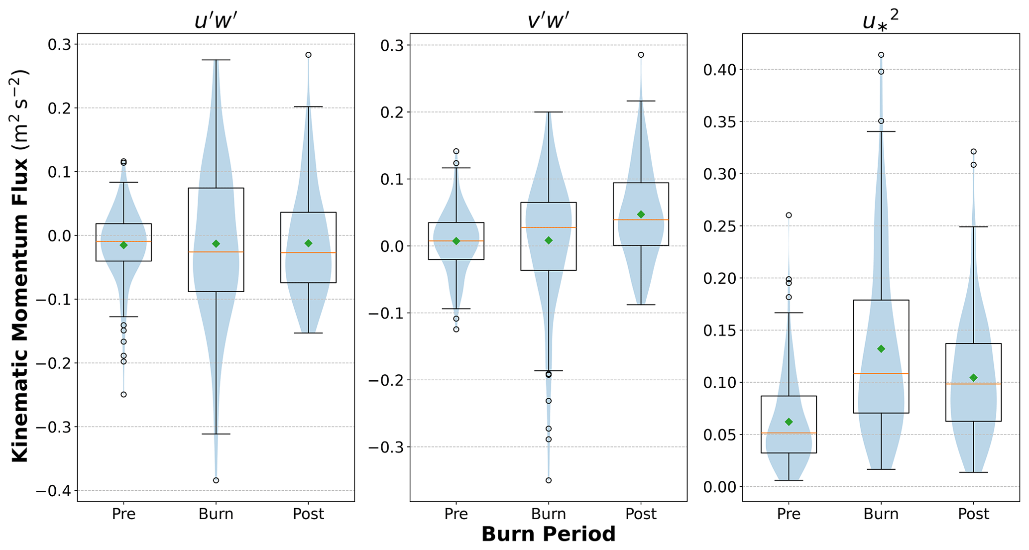
Figure 11 Distributions of friction velocity squared ($u_{\ast }^{\mathrm{2}}$) and its two components ($\stackrel{\mathrm{‾}}{u^{\prime }{w}^{\prime }}$ and $\stackrel{\mathrm{‾}}{v^{\prime }{w}^{\prime }}$) from all 16 sonic anemometers during the pre-burn, burn and post-burn periods. The box represents the 25th and 75th percentile of the data, with data inside the whiskers representing 99.3 % of the data. The orange line in the boxes is the median value, the green diamond is the mean and the blue shading is the density of values of the data.

The overall distributions of $u_{\ast }^{\mathrm{2}}$, $\stackrel{\mathrm{‾}}{u^{\prime }{w}^{\prime }}$ and $\stackrel{\mathrm{‾}}{v^{\prime }{w}^{\prime }}$ from all 16 sonic anemometers are depicted in Fig. 11. During the pre-burn period, $\stackrel{\mathrm{‾}}{u^{\prime }{w}^{\prime }}$ is negative, with a mean value of −0.015 m² s⁻², indicating an overall downward transfer of higher streamwise momentum air, which is expected as wind speed usually increases with height. The mean of the cross-stream momentum flux $\stackrel{\mathrm{‾}}{v^{\prime }{w}^{\prime }}$ is near zero (0.007 m² s⁻²). However, the spread of the two components is similar, with standard deviations of 0.057 and 0.046 m² s⁻² for $\stackrel{\mathrm{‾}}{u^{\prime }{w}^{\prime }}$ and $\stackrel{\mathrm{‾}}{v^{\prime }{w}^{\prime }}$, respectively. The pre-burn stress $u_{\ast }^{\mathrm{2}}$ of 0.061 m² s⁻² (u_∗ = 0.25 m² s⁻²) is typical for daytime surface layers.

An increase in the downward (upward) transfer of higher streamwise (cross-stream) momentum is observed during the burn period as the median values become more negative for $\stackrel{\mathrm{‾}}{u^{\prime }{w}^{\prime }}$ and more positive for $\stackrel{\mathrm{‾}}{v^{\prime }{w}^{\prime }}$. However, the mean values change little from the pre-burn period. The spread is doubled from a standard deviation of 0.046 to 0.098 m² s⁻² for $\stackrel{\mathrm{‾}}{u^{\prime }{w}^{\prime }}$ and nearly tripled from 0.05 to 0.124 m² s⁻² for $\stackrel{\mathrm{‾}}{v^{\prime }{w}^{\prime }}$. The stronger upward transfer of cross-stream momentum is consistent with the generation of cross-stream wind and updrafts in the vicinity of the surface fire. Despite this overall fire-induced increase in $\stackrel{\mathrm{‾}}{v^{\prime }{w}^{\prime }}$, the distribution of the cross-stream momentum is negatively skewed by large negative outliers, suggesting occasional transfer of higher cross-stream momentum by downdrafts near the vicinity of the fire. Both the mean and standard deviation of $u_{\ast }^{\mathrm{2}}$ values are doubled to 0.13 and 0.086 m² s⁻², respectively, over the pre-burn values. The peak 1 min averaged values of $u_{\ast }^{\mathrm{2}}$ exceed 0.4 m² s⁻² (or a friction velocity of 0.6 m s⁻¹), which is 2.5 times larger than the pre-burn values. Clements et al. (2008) also observed a 3-fold increase in friction velocity in their experiment involving a high-intensity grass fire, although the absolute values of the friction velocity in their experiment were 5 times larger (1 and 3 m s⁻¹ before and during the fire) than the current experiment.

The mean post-burn $u_{\ast }^{\mathrm{2}}$ value (0.10 m² s⁻²) is lower than that of the burn period but still higher than the pre-burn value, driven primarily by the cross-stream component. The values of the $\stackrel{\mathrm{‾}}{v^{\prime }{w}^{\prime }}$ (0.0471 m² s⁻²) in the post-burn period are more than 6 times the pre-burn average (0.0072 m² s⁻²), with a standard deviation (0.069 m² s⁻²) that is between the pre-burn period (0.046) and burn period (0.096) values. The mean friction velocity therefore does not return to the pre-burn average, although it is lower than the average during the burn period. Other experiments (e.g., Clements et al., 2008; Heilman, et al. 2019) noted a return of friction velocity to pre-burn values soon after the passage of the fire front, during a period when smoldering was occurring. The results of this analysis suggest that friction velocities do not quickly return to pre-burn values on all fires.

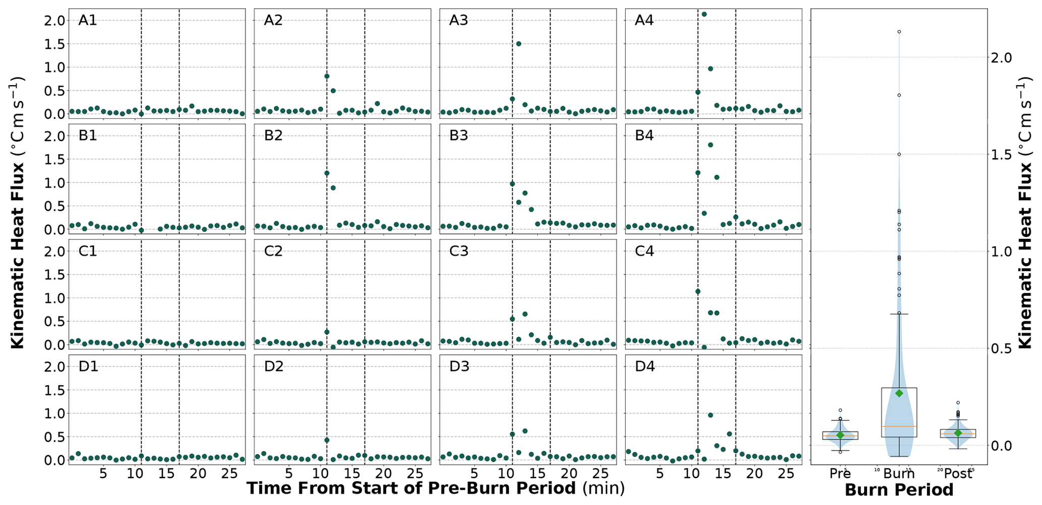
Figure 12 Time series of 1 min averaged heat flux for each of the 16 sonic anemometers (left) and the distribution of heat fluxes from all 16 sonic anemometers during the pre-burn, burn and post-burn periods (right). The box represents the 25th and 75th percentile of the data, with data inside the whiskers representing 99.3 % of the data. The orange line in the boxes is the median value, the green diamond is the mean and the blue shading is the density of values of the data.

3.4 Fire-induced turbulent heat flux

We proceed to examine the impact of the fire on turbulent heat flux. Time series of 1 min average kinematic turbulence sensible heat flux $\stackrel{\mathrm{‾}}{T^{\prime }{w}^{\prime }}$ for each sonic anemometer are shown in Fig. 12 for the three periods, which also shows the overall distribution of heat fluxes for all the sonic anemometers. In the pre-burn period, the sonic anemometers recorded background $\stackrel{\mathrm{‾}}{T^{\prime }{w}^{\prime }}$ values that averaged around 5.25 × 10⁻² ${}^{\circ }\mathrm{C}\mathrm{m}{\mathrm{s}}^{-\mathrm{1}}$ (or 52.7 W m⁻² after multiplying by the density and heat capacity of air), with a standard deviation of 3.41 × 10⁻² ${}^{\circ }\mathrm{C}\mathrm{m}{\mathrm{s}}^{-\mathrm{1}}$ (34 W m⁻²). During the burn period, a fire-induced increase in $\stackrel{\mathrm{‾}}{T^{\prime }{w}^{\prime }}$ is evident for all but the westernmost sonic anemometers (A1, B1, C1 and D1), with larger increases appearing at the easternmost locations. The largest $\stackrel{\mathrm{‾}}{T^{\prime }{w}^{\prime }}$ values generally occur early in the burn period, with the A4 sonic having the largest $\stackrel{\mathrm{‾}}{T^{\prime }{w}^{\prime }}$ value of 2.13 ${}^{\circ }\mathrm{C}\mathrm{m}{\mathrm{s}}^{-\mathrm{1}}$ (2.138 kW m⁻²). Based on the IR imaging (Fig. 4), after the first 3 min of the burn period, there is a slight shift in the burn direction towards the southeastern side of the plot. This shift in direction is apparent in the time series for the D4 sonic anemometer, which is located on the southeastern corner of the burn plot, where elevated $\stackrel{\mathrm{‾}}{T^{\prime }{w}^{\prime }}$ values are recorded late in the burn period, at a time when the values have dropped at most of the other sonic anemometers. The overall distribution of the burn-period $\stackrel{\mathrm{‾}}{T^{\prime }{w}^{\prime }}$ is skewed by larger values since the plot mean was 0.268 K m s⁻¹ (269 W m⁻²), but the median was just 0.0974 ${}^{\circ }\mathrm{C}\mathrm{m}{\mathrm{s}}^{-\mathrm{1}}$(98 W m⁻²).

Values of $\stackrel{\mathrm{‾}}{T^{\prime }{w}^{\prime }}$ during the post-burn period quickly drop back to just slightly above the pre-burn values, with a mean of 6.35 × 10⁻² ${}^{\circ }\mathrm{C}\mathrm{m}{\mathrm{s}}^{-\mathrm{1}}$ (64 W m⁻²) and a standard deviation of 3.76 × 10⁻² ${}^{\circ }\mathrm{C}\mathrm{m}{\mathrm{s}}^{-\mathrm{1}}$ (38 W m⁻²). However, the post-burn period contains several outliers (above the 99.3 % percentile), indicating the influence of smoldering on some of the sonic anemometers even after the fire has exited the burn plot. A specific example of the smoldering effect is the D4 sonic anemometer, where the post-burn $\stackrel{\mathrm{‾}}{T^{\prime }{w}^{\prime }}$ (0.126 ${}^{\circ }\mathrm{C}\mathrm{m}{\mathrm{s}}^{-\mathrm{1}}$ or 126 W m⁻²) is about twice the pre-burn value. The overall modest increase in $\stackrel{\mathrm{‾}}{T^{\prime }{w}^{\prime }}$ in the post-burn period compared to the pre-burn period was also observed in the two wildland fire experiments described in Heilman et al. (2019).

3.5 Quadrant analyses

3.5.1 Turbulent heat fluxes

The analysis above provided a quantitative assessment of fire-induced changes to the turbulent heat and momentum fluxes through comparisons of flux values between the pre-burn and the burn periods. However, such analysis cannot reveal what types of heat or momentum transfer events are mostly affected by the fire. We apply the quadrant analysis method (also known as sweep–ejection analysis) described earlier (Table 1) to the observed turbulent fluxes to provide additional insight into how the fire changes the composition of heat and momentum fluxes. By partitioning the total heat and momentum fluxes into four quadrants representing different types of flux events, the quadrant or sweep–ejection analysis allows for the delineation of the fire influence on specific types of turbulent heat and momentum transfer processes.

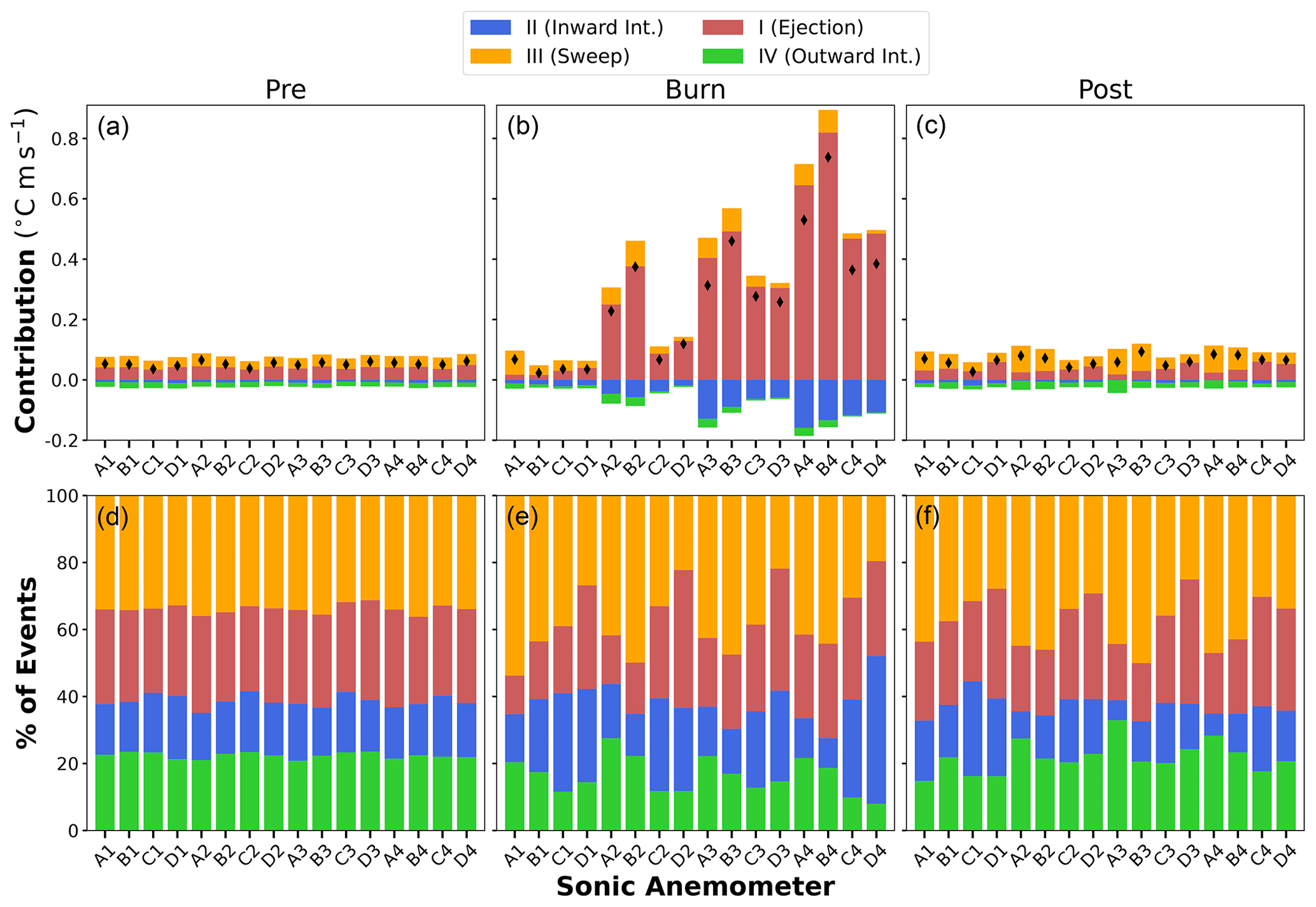
Figure 13 Quadrant analysis of the instantaneous vertical kinematic turbulent heat fluxes showing the contributions to the total flux from (a–c) and the percent of (d–f) the four types of events, outward interaction (green), ejection (red), inward interaction (blue) and sweep (orange), for each of the 16 sonic anemometers during the pre-burn, burn and post-burn periods. The black diamonds in (a–c) indicate the total heat flux values. The sonic anemometers are arranged from west to east, roughly following the fire spread across the burn plot.

Figure 13 shows the relative contributions and the proportional number of occurrence of the different heat flux events (i.e., sweeps, ejections, outward interactions and inward interactions) during each period, observed by each of the 16 sonic anemometers. During the pre-burn period, the partitioning among the four types of events (see Table 1) by contribution and proportion exhibits little variation across the 16 sonic anemometers. At all locations, the ejection and sweep events dominate, accounting for over 60 % of the total events, with sweep being slightly larger. The rest is split between outward interaction and inward interaction events, with the former slightly outnumbering (20 %–23 %) the latter (14 %–19 %). A similar partitioning is observed for the event contributions for the heat fluxes, but the ejection events, despite being slightly less frequent, contribute more to the heat flux than do the sweep events. This apparent inconsistency between the partitioning of the event number and the event contribution suggests that ejection events likely involve larger eddies and stronger heat transfer compared to sweep events. This pre-burn period partitioning is similar to previous ambient daytime measurements observed in other studies (e.g., Heilman et al., 2021).

The burn period is marked by substantial heterogeneity across the 16 sonic anemometers. Despite differences in the magnitudes of contributions to the heat fluxes amongst the sonic anemometers, the increases in the overall positive mean heat flux during the burn period can be largely attributed to increases of ejection events that contribute to positive heat fluxes through upward transfer of warmer air from the combustion zone to the atmosphere above. There is also an increase in the negative contribution from inward interaction events, which represents the downward transfer of warmer air from the atmosphere to the combustion zone. The contributions to the overall mean heat flux by the other two types of events, sweep and outward interaction, show little change from the pre-burn to the burn periods, which suggests that the turbulent heat transfer processes represented by these types of events, namely downward transfer of colder air from above to the surface or upward transfer of colder air from the combustion zone to the atmosphere, are not very sensitive to the presence of a low-intensity fuel-bed-scale surface fire.

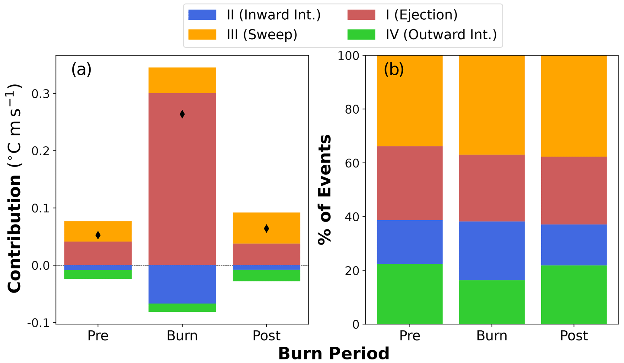
Figure 14 Quadrant analysis of the instantaneous vertical kinematic turbulent heat fluxes showing (a) the contributions to the total flux and (b) the percent of the four types of events, outward interaction (green), ejection (red), inward interaction (blue) and sweep (orange), for all 16 sonic anemometers during the pre-burn, burn and post-burn periods. The black diamonds in (a) indicate the total heat flux values.

Compared to the partitioning in event contribution, the fire-induced changes to the partitioning in event number are less clear. In general, the sonic anemometers that show an increase in the contribution by inward interaction events also exhibit an increase in the number of inward interaction events from the pre-burn to the burn periods. However, an increased contribution to the overall mean heat flux by ejection events does not correspond to an increase in the number of the ejection events. The increased number of sweep events is in agreement with the increased sweep contributions at several sonics (A2–A4 and B2–B4), although the sweep contributions are overwhelmed by ejection contributions at these sonic anemometers.

A key finding from this heat flux sweep–ejection analysis is that turbulent heat fluxes during the burn period are overwhelmingly dominated by ejection events, but there is usually a small or no increase in the number of ejection events. This suggests that the presence of a low-intensity fuel-bed-scale fire does not necessarily produce more upward turbulent heat transfer events, but instead, it produces stronger events that quickly transfer and diffuse the sensible heat generated by combustion into the ambient atmosphere above.

During the post-burn period, most sonic anemometers show vertical heat flux values that are smaller than the burn period but still larger than the pre-burn period. The largest contribution to the overall mean heat flux is usually from sweep events, accompanied also by an increase in the number of the events, indicating the occurrence of many events where cold air is transferred downward. The post-burn period also exhibits an increase in the heat flux contributions from outward interaction events, which represent downward transfer of warm air. Similar to the burn period, inward interaction events, both in contribution and number, vary considerably across the sonic array.

Figure 14 shows the partitioning of both the event number and the event contribution to turbulent heat fluxes using data from all 16 sonic anemometers, which highlights more clearly how the fire modifies the overall heat flux regime. Similar to the heat flux quadrant analysis for individual sonic anemometers, the heat flux events averaged across the sonic anemometer array for the pre-burn period are dominated by sweep (32 %) and ejection (28 %) events. Inward interaction events occur with the least proportion (17 %), followed by outward interaction events (23 %). The sweep and ejection events, which contribute to positive heat fluxes, are much larger in magnitude than the negative heat flux contributions from the inward and outward interaction events. The dominance of sweep and ejection events for the turbulent heat fluxes during the pre-burn period follows observations made in previous studies (Heilman et al., 2021).

The combined proportions of sweep and ejection events (both contributing to positive heat fluxes) and the outward and inward interaction events (both contributing to negative heat fluxes) remain similar between the burn and the pre-burn period. However, between the two types of events in each group, one (sweep, inward interaction) increases, and the other (ejection, outward interaction) decreases in proportion. Previous fire experiments also reported an increase in sweep events and a generally proportional decrease in ejection events (Heilman et al., 2021), but the magnitudes of the changes are larger than what is observed here, likely because the previous fires were more intense. Additionally, modest changes in the partitioning of the event number and contributions for this fire could be a byproduct of combining data from sonic anemometers that are not strongly affected by the fire front (i.e., the westernmost sonic anemometers) with those that experience more substantial changes.

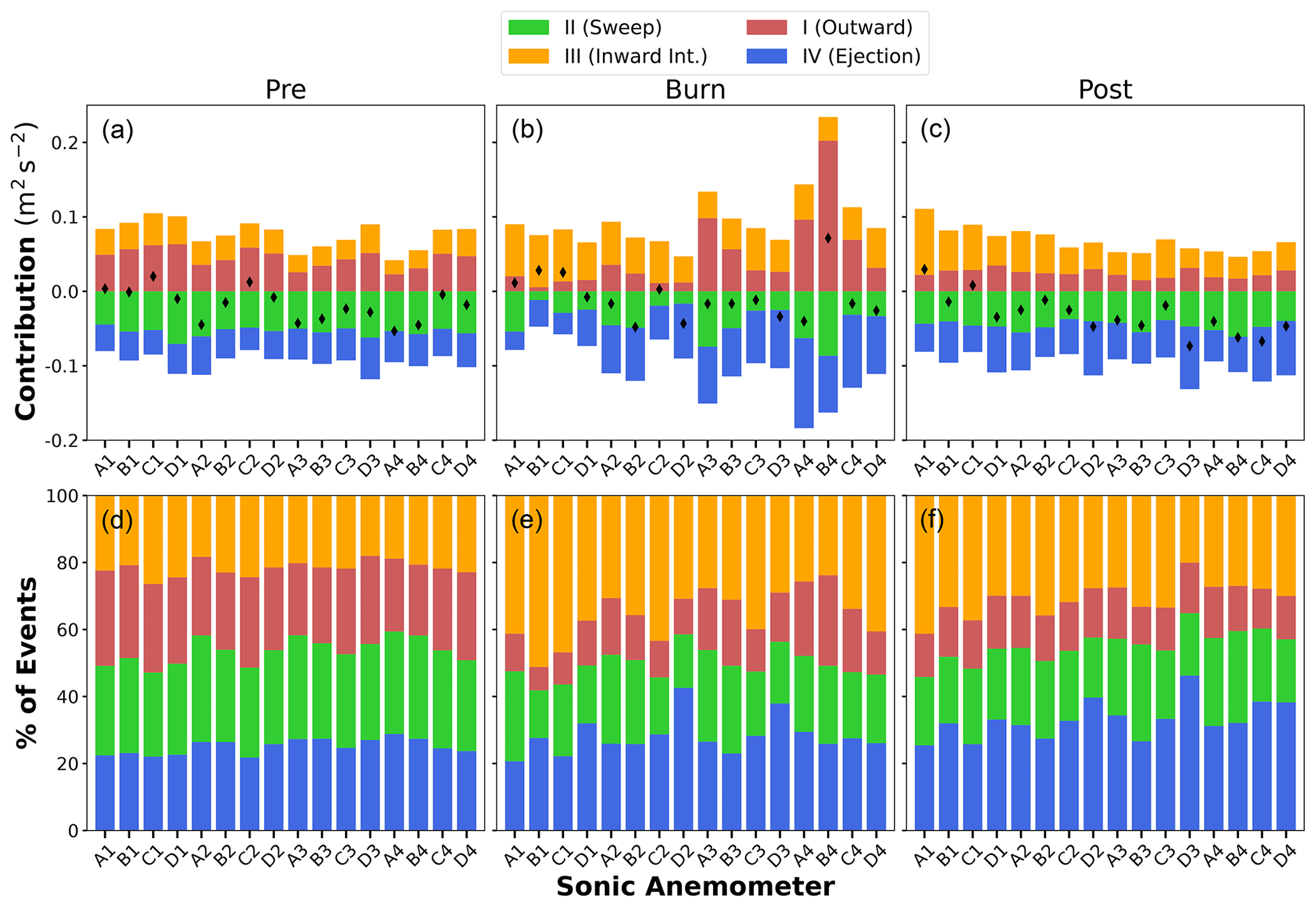
Figure 15 Quadrant analysis of the instantaneous vertical kinematic turbulent fluxes of horizontal momentum showing the contributions to the total flux from (a–c) and the percent of (d–f) the four types of events, outward interaction (red), sweep (green), inward interaction (orange) and ejection (blue), for each of the 16 sonic anemometers during the pre-burn, burn and post-burn periods. The black diamonds in (a–c) indicate the total flux values. The sonic anemometers are arranged from west to east, roughly following the fire spread across the burn plot.

The large changes in the contributions of the heat flux events during the burn period suggest that this fire has greater impacts on the event contributions to the mean turbulent heat fluxes than on the event number. Specifically, ejection event contributions dominate in the burn period, making up 70.4 % of the total contribution, while sweep and outward interaction contributions decrease by a third and a sixth, respectively, compared to their contributions during the pre-burn period. The magnitude of the contribution from inward interaction events increases slightly but is quite similar to the contribution during the pre-burn period.

Heat flux events in the post-burn period more closely resemble the pre-burn period than the burn period, but the event contributions and the event number do not return entirely to their pre-burn values. As noted in the analyses of TKE and kinematic heat flux (Figs. 9 and 11), this result is consistent with smoldering occurring in the burn plot during the post-burn period. The sweep event contribution during the post-burn period is 1.5 times higher than during the pre-burn period and 1.3 times higher than during the burn period. Compared to the pre-burn values, the post-burn period event contributions are slightly higher for outward interaction events and slightly lower for ejection and inward interaction events. Overall, the post-burn period is dominated by contributions from sweep events (37.7 %), which is followed by ejection events (25.3 %) although lower than pre-burn values. These results differ somewhat from Heilman et al. (2021) in that they reported both sweep and ejection events returning to pre-burn values, while only ejection events return to pre-burn values for this fire.

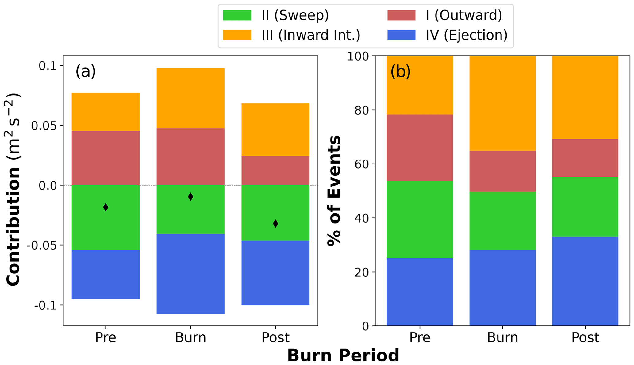
Figure 16 Quadrant analysis of the instantaneous vertical kinematic turbulent fluxes of horizontal momentum showing (a) the contributions to the total flux and (b) the percent of the four types of events, outward interaction (red), sweep (green), inward interaction (orange) and ejection (blue), for all 16 sonic anemometers during the pre-burn, burn and post-burn periods. The black diamonds in (a) indicate the total flux values.

3.5.2 Turbulent momentum fluxes

Quadrant analysis is also applied to partition the vertical turbulent kinematic flux of horizontal momentum $\stackrel{\mathrm{‾}}{S^{\prime }{w}^{\prime }}$ into four different types, and the results for each of the 16 sonic anemometers are shown in Fig. 15. During the pre-burn period, the overall mean momentum fluxes are negative at all but two sonic anemometers (C1, C2), where the flux is slightly positive. Between the two types of events that contribute to negative momentum fluxes, the sweep events (downward transfer of higher horizontal momentum air from the atmosphere to the combustion zone) contribute more than the ejection events (upward transfer of lower horizontal momentum air from the combustion zone to the atmosphere above), which is consistent with the slightly higher number of sweep events than ejection events. Between the two types of events that contribute to positive momentum fluxes, the outward interaction events (upward transfer of higher horizontal momentum air from the combustion zone to the atmosphere above) contribute more than the inward interaction events (downward transfer of lower horizontal momentum air from the atmosphere to the combustion zone), although the number of the inward and outward interaction events is similar.

The changes from the pre-burn period to the burn period vary substantially by location, but the sign of the overall mean momentum fluxes remains unchanged at most locations. The most pronounced and consistent change across the anemometer array is a substantial increase in the proportional number of inward interaction events and, to a lesser degree, the contribution from these events. The ejection events also exhibit an increase in the number and the contribution at most of the sonic anemometer locations. There is a general decrease in the number of sweep and outward interaction events, but the contributions are not consistent, with some sonic anemometers showing an increase while others experience a decrease in contribution.

An exception to the above general observations between the pre-burn and burn periods is B4, where the overall momentum flux shifts from negative to positive due to an increase in outward interaction contribution by as much as 5 times the pre-burn magnitude. The amount of increase in the contribution from the outward interaction events, however, does not match the small increase (approximately 10 %) in the event number, which suggests that the increase in the overall momentum flux magnitude at this location is likely due to a small number of extremely strong events of upward transfer of higher horizontal momentum air associated with large, energetic eddies generated by the surface fire.

The large heterogeneity in the event contribution values for the momentum fluxes across the sonic anemometer array during the burn period dissipated substantially into the post-burn period. The event contribution and event number distributions once again become less dependent on the locations of the sonic anemometers. Despite this tendency to return to the pre-burn distribution, the post-burn period experiences larger contributions from and a higher number of ejection and inward interaction events than sweep and outward interaction events, which is opposite to the pre-burn period and similar to the burn period.

Figure 16 shows a quadrant analysis that combines data from all the sonic anemometers, which allows for an assessment of how the fire modified the momentum flux turbulence regime for the entire burn plot. Overall, sweep (31.9 %) and outward interaction (26.6 %) events dominate the momentum flux contributions in the pre-burn period. The increases in the proportion of inward interaction and ejection events from the pre-burn to the burn periods make the contributions more balanced across the four quadrants, suggesting that the different event contributions are more similar to each other during the burn than the pre-burn period. In the post-fire period, inward interaction events contribute more to the mean momentum flux (25.7 %) than during the pre-fire period (18.1 %). The event number distributions in the combined analysis echoes the results from the individual sonic anemometers, with the pre-burn period showing similar values for all four quadrants, a sharp increase in inward interaction events and decrease in outward interaction events during the burn period, and fewer inward interaction events during the post-burn period than during the burn period but more numerous than during the pre-burn period.

The results of the quadrant analysis of momentum fluxes presented above are somewhat different from those of previous studies involving operational-scale prescribed burns. Heilman et al. (2021) showed that during an intense grass fire and two low-intensity forest understory fires, there can be substantial increase in the number and contribution of sweep and outward interaction events and that the increase in the positive momentum flux from outward interaction events largely offsets the increase in the negative flux associated with sweep events, whereas in the small fuel-bed-scale burn here, inward interactions occur most frequently, followed by ejection events. However, the ejection event contributions to the mean momentum flux are larger (32.3 %), with the inward interaction event contributions (24.2 %) more similar to the outward interaction (23.4 %) contributions. The feature of increased frequency of inward interaction events and their increased contribution to the mean momentum flux compared to previous burns is further observed in the post-burn period.

The event number and event contributions during the post-burn period also differ with increased ejection and inward interactions events, 32.8 % and 20.6 %, while the large-scale burns in Heilman et al. (2021) showed a closer return to pre-fire periods, with sweep and ejection events making up the majority of event number and contributions. The contributions from sweep, inward interaction and ejection events remain elevated during the post-burn period, while the contributions from outward interaction decrease during post-burn to values lower than the values of the pre-burn period.

4 Summary

This study presents the atmospheric turbulence dynamics observed through a 4 × 4 array of fast-response 3D sonic anemometers during a low-intensity fire experiment on a 10 m × 10 m burn plot in the Silas Little Experimental Forest in New Jersey, USA. The density of turbulence measurements is unprecedented for fire experiments, allowing for a deeper analysis of heterogeneities as the surface line fire spread through the burn plot than was previously possible. The analysis focuses on assessments of the fire impacts on turbulence intensity, as measured by TKE, turbulent momentum flux or shear stress as measured by friction velocity, and turbulent heat flux.

The influence of the low-intensity surface line fire on the atmosphere above the combustion zone is evidenced by an increase in temperature up to 20 ^∘C; the generation of strong updrafts up to 6 m s⁻¹ and downdrafts up to −5 m s⁻¹; and a decrease in the streamwise velocity coupled with an increase in the cross-stream velocity, indicating horizontal convergence in the vicinity of the fire front. The observed fire exhibited behavior more consistent with a buoyant plume than mechanically forced rising motion resulting from converging surface air. The influence of the fire on horizontal velocity components persisted longer after fire front passage, while the influence on vertical velocity subsided rapidly behind the fire front.

The fire modified turbulence characteristics at the fuel bed–atmosphere interface. There was an increase in the turbulence intensity, with TKE values 2–3 times higher than the ambient environment, due primarily to the increase in cross-stream velocity variance and, to a lesser degree, the increase in the vertical velocity and streamwise velocity variance. Heilman et al. (2017) also reported 2- to 3-fold increases in TKE values during two operational-scale low-intensity forest understory prescribed fires. It is interesting to note that this increase in TKE is only slightly smaller than what was observed during the intense grass fire during FireFlux (Clements et al., 2007), although the magnitude of TKE of the intense grass fire is substantially larger than that of the low-intensity fires. Despite this increase in TKE, the value of TKE was still smaller than what is expected in an environment of substantial turbulence. Additionally, despite the increase in the vertical velocity variance during the fire, the TKE was still dominated by the horizontal velocity variance, indicating that the turbulence regime remained anisotropic (anisotropic ratio < $\mathrm{1}/\mathrm{3}$) above the combustion zone of this low-intensity fuel-bed-scale surface fire.

The fire enhanced upward sensible heat fluxes substantially by as much as 40 times the flux in the ambient atmosphere (from 50 W m⁻² to 2 kW m⁻²). This change in the sensible heat flux is largely attributable to an increased contribution of upward transfer by turbulent eddies of warmer air from the combustion zone to the atmosphere above, which is also known as ejection events for vertical turbulent heat transfer. This increase in the contribution of the ejection events to turbulent heat fluxes was not caused by a corresponding increase in the number of ejection events that changed little from the pre-burn to burn periods. This mismatch between the ejection event contribution and event number suggests that the presence of a low-intensity fuel-bed-scale fire may not necessarily produce more upward turbulent heat transfer events, but rather, it can produce strong ejection events associated with large, energetic eddies. The warmer air transported upward by the ejection events can also be transported downward by inward interaction events, which also increased somewhat during the fire.

Compared to the turbulent heat flux, the impact of the fire on turbulent momentum flux or shear stress was less pronounced. In general, an increase in momentum fluxes was observed during the burn, with friction velocity, a measure of total shear stress on horizontal wind, 2–3 times the ambient value (from ∼ 0.25 to 0.6 m s⁻¹). Previous studies of operational-scale grass fire or forest understory fires also found up to a 3-fold increase in friction velocity, despite the scale of this fire being much smaller than the previous fires and the absolute values of friction velocity during the intense grass fire being 5 times higher than the low-intensity fire here (Clements et al., 2007; Heilman et al., 2017; 2021). The fire was accompanied by an increase in the downward transfer of lower horizontal momentum air, also known as inward interaction events, along with a smaller increase in the upward transfer of lower horizontal momentum air referred to as ejection events. This finding differs from previous observations during an operational-scale forest understory fire, where an increase in sweep (downward transfer of higher horizontal momentum air) and outward interaction (upward transfer of higher horizontal momentum air) contributions to the mean momentum fluxes was detected (Heilman et al., 2021).

These findings directly address the initial research inquiries: how does the surface fire impact turbulence intensity and the exchanges of turbulent heat and momentum between the combustion zone and the atmosphere above? Additionally, the investigation delves into how the presence of fire alters the distribution of heat and momentum fluxes into different event types, considering both event number and contribution.

Perhaps the most significant finding from this study is the large variations in the observed fire-induced perturbations across the sonic anemometer array in the burn plot. This directly corresponds to the third question raised in the introduction: how do the fire-induced modifications on turbulence vary spatially across the burn plot? The anemometers on the western side of the burn plot where a surface line fire was ignited picked up very weak or no signals of the fire despite the proximity to the initial fire line. In contrast, the sonic anemometers in the center or eastern side of the burn plot picked up clear fire signals. Although the features of fire-induced turbulence regime (e.g., anisotropy, sweep–ejection dynamics) revealed by the sonic anemometers are similar, the magnitudes vary with downwind distance and the relative position of the sonic anemometers to the impinging fire front. Considering the size of the burn plot (10 m × 10 m) and the homogeneity of consumed fuels, this finding suggests that considerable care should be taken when comparing, contrasting and combining data from multiple fires or from multiple instruments on the same fire to ensure that significant fire signals are not being over- or under-represented in the analyses that inform the conclusions of the studies. This also calls into question the use of numerical simulations from coupled atmosphere–fire behavior models with horizontal grid spacing ≥ 10 m. The results presented here suggest that 1–2 m grid spacing is necessary for model simulations to capture atmospheric turbulent circulations that have spatiotemporal scales similar to the scales associated with flame dynamics in the combustion zone. It is, however, impractical for operational applications to use such fine resolution. Operational models, with resolutions ranging from tens to hundreds of meters, often fall within the so-called “gray zone” where turbulence is partially resolved, and existing turbulence closure schemes designed to parameterize all turbulent motions are inadequate. Advancements in computing technology have brought this zone to the forefront of operational model simulations. Developing turbulence closure schemes for this scale is an active area of research. Large-eddy-simulation (LES) models, validated using laboratory data, are instrumental in this endeavor. The experiments described in this study, capturing fire-induced turbulence on a 10 m × 10 m plot, can play a crucial role in developing turbulence parameterizations for the gray zone when combined with LES models.

Future work will compare results from this case with those of other burns in the SERDP 10 m × 10 m fuel-bed-scale burn series to delineate the effect of fuel and ambient atmospheric conditions on fire–atmosphere interactions and with results from other prescribed-fire experiments to help scale up or scale down the results between small-scale and operational-scale fires. Future work will also include the reanalysis of 10 Hz sonic anemometer data from other fire experiments using some or all of the methodologies employed here, which could contribute to the identification and documentation of a series of steps, protocols, standards and methodologies by which 10 Hz sonic anemometer data collected during fire experiments can be compared and contextualized. Additionally, forthcoming analyses will integrate data collected from other instruments deployed during these fuel-bed-scale fire experiments. For instance, examining the high-frequency thermocouple vertical profile (0, 5, 10, 20, 30, 50, 100 cm) in conjunction with infrared data can offer significant insights into the vertical variation of temperature between the combustion zone and the atmosphere immediately above. Finally yet importantly, employing spectral and co-spectral analyses will be essential in revealing the temporal and spatial scale of turbulence regimes at the fuel bed–atmosphere interface. These analyses will simultaneously enable a holistic exploration of the oscillatory behavior tied to line fires.

Another facet to delve into in future research involves the generation of vorticity, a consequential byproduct of fires that significantly influences fire behavior. Estimating fire-induced vorticity from field observations presents a formidable challenge, necessitating a carefully designed instrument array capable of capturing both horizontal and vertical variations in wind velocity. Despite these challenges, the utilization of the 4x4 sonic anemometer array in the 10 m × 10 m burn plot provides a distinctive opportunity. This array captures horizontal variations in wind velocity as the line fire spreads through the plot, offering a unique opportunity for estimating vertical vorticity associated with line fires. However, it is important to note that estimating horizontal vorticity is not feasible due to the sonic anemometer array's velocity measurement on a single vertical level (2.5 m), which does not capture the necessary vertical variations of velocity for horizontal vorticity calculation. Future experiments will require the deployment of a densely spaced sonic anemometer similar to the current one but at multiple vertical levels to comprehensively evaluate vorticity associated with fires.

Finally, it is worth mentioning that because the burn period was chosen to be between the time when the first and the last sonic anemometers have temperatures satisfying the threshold value (eight standard deviations in these analyses), the burn period included time after the fire has passed the sonic anemometer location, which likely yielded an underestimation of the fire effect. Similarly, the inclusion of all 16 sonic anemometers in the analysis, including those that registered little fire signal, likely contributed to an underestimation. Consequently, fire-induced turbulent circulations and the associated turbulent heat and momentum fluxes are likely to be stronger than what has been reported here.