The co-benefits of a low-carbon future for PM_2.5 and O₃ air pollution in Europe

There is considerable academic interest in the potential for air quality improvement as a co-benefit of climate change mitigation. Few studies use regional air quality models for simulating future co-benefits, but many use global chemistry–climate model output. Using regional atmospheric chemistry could provide a better representation of air quality changes than global chemistry–climate models, especially by improving the representation of elevated urban concentrations. We use a detailed regional atmospheric-chemistry model (WRF-Chem v4.2) to model European air quality in 2050 compared to 2014 following three climate change mitigation scenarios. We represent different climate futures by using air pollutant emissions and chemical boundary conditions (from CESM2-WACCM output) for three shared socioeconomic pathways (SSP1-2.6, SSP2-4.5 and SSP3-7.0: high-, medium- and low-mitigation pathways respectively).

We find that in 2050, following SSP1-2.6, mean population-weighted PM_2.5 concentrations across European countries are reduced by 52 % compared to 2014. Under SSP2-4.5, this average reduction is 34%. The smallest average reduction is 18 %, achieved following SSP3-7.0. Maximum 6-monthly-mean daily-maximum 8 h (6mDM8h) ozone (O₃) is reduced across Europe by 15 % following SSP1-2.6 and by 3 % following SSP2-4.5, but it increases by 13 % following SSP3-7.0. This demonstrates clear co-benefits of climate mitigation. The additional resolution allows us to analyse regional differences and identify key sectors. We find that the mitigation of agricultural emissions will be key for attaining meaningful co-benefits of mitigation policies, as evidenced by the importance of changes in NO₃ aerosol mass to future PM_2.5 air quality and changes in CH₄ emissions to future O₃ air quality.

1 Introduction

Air pollution is a major public-health issue worldwide. The health impacts are usually attributed to two air pollutants – PM_2.5 (any airborne non-gaseous particle under 2.5 µm in diameter), which can be both a primary or secondary air pollutant, and ozone (O₃), which is a secondary pollutant. Primary sources of PM_2.5 include a range of natural and anthropogenic sources. As a secondary pollutant, it can be formed from emissions of species such as ammonia (NH₃), sulfur dioxide (SO₂) and nitrogen oxides (NO_x). Tropospheric O₃ is a secondary pollutant formed by photochemical reactions involving volatile organic compounds (VOCs), including methane (CH₄), nitrogen oxides (NO_x) and carbon monoxide (CO), in the presence of sunlight. Air pollution has wider consequences than just mortality, such as the economic cost (Vandyck et al., 2020) and reduced crop yields (Lobell et al., 2022). Both PM_2.5 and O₃ are linked with climate change; many sources of primary PM_2.5 and O₃ precursors are also sources of long-lived greenhouse gases. Additionally, air pollutants themselves have an impact on climate forcing through several pathways, including by directly affecting the radiative balance of the atmosphere, modifying the albedos of clouds and glaciers, and increasing the cloud lifetime (von Schneidemesser et al., 2020; Peace et al., 2020).

Exposure to air pollution contributes to about 6.7 million deaths per year (World Health Organisation, 2022), 4.2 million of which are from ambient outdoor air pollution. In Europe, an estimated 368 000 deaths per year are attributable to air pollution according to Juginovic et al. (2021), approximately 90 % of which were attributable to PM_2.5, and the annual mean mortality rate from air pollution in Europe of 133 deaths per 100 000 people exceeds the global mean of 120 deaths per 100 000 (Lelieveld et al., 2020). Additionally, the European Environment Agency (2022) reported that in 2022, 96 % of Europe's urban population was exposed to PM_2.5 concentrations above the World Health Organisation's guideline value of 5 µg m⁻³ (World Health Organisation, 2021).

Improving air quality in Europe is feasible: primary air pollution responds quickly to air pollutant emissions reductions, potentially resulting in lower population exposure. Notably, some secondary air pollutants such as O₃ can worsen depending on the emissions reductions in some circumstances, but reducing emissions largely leads to an overall air quality benefit. Due to reductions in anthropogenic emissions of air pollutants, the PM_2.5 air quality in most of Europe has improved over the past half-century; between 1960 and 2009, population-weighted PM_2.5 concentrations in the European Union decreased by 55.3 % (Butt et al., 2017). Similarly, the responsiveness of air pollution to emissions changes was demonstrated by the changes in PM_2.5 air quality from national to global scales during the COVID-19 pandemic (Jephcote et al., 2021; Venter et al., 2021; Putaud et al., 2023). The speed of this response to changes in emissions indicates that considerable improvements in air quality can be achieved when air pollutant emissions are reduced. Conversely, O₃ concentrations in Europe have increased in the latter half of the 20th century and early 21st century (Turnock et al., 2020) despite considerable reductions in local anthropogenic O₃ precursor emissions. This is potentially due to increased intercontinental transport of O₃ precursors (Guerreiro et al., 2014). Despite improving trends in PM_2.5, O₃ concentrations may increase because reduced NO_x emissions result in the reduced titration of O₃ (Miyazaki et al., 2021). A different approach may therefore be required to reduce exposure to O₃.

Greenhouse gas mitigation policies may also result in lower air pollution emissions and subsequent improved air quality (Turnock et al., 2020; Vandyck et al., 2020). This co-benefit is often suggested as a motivator to encourage faster and stronger climate mitigation from policymakers, including at the regional level, because it turns the concept of climate change mitigation from a diffuse, global-scale requirement to something that can provide measurable near-term local benefits (von Schneidemesser et al., 2020). Existing research suggests that air quality co-benefits of climate mitigation could occur in Europe. For example, Turnock et al. (2020) find that across Europe, PM_2.5 concentrations would decrease by the middle of this century for a range of future scenarios and be lower in scenarios with greater mitigation. Reddington et al. (2023) find that reductions in PM_2.5 across Europe following a sustainable scenario (SSP1-1.9) could improve health across the continent. Fenech et al. (2021) find similar when focusing on the UK. This may not be true for all pollutants and all scenarios. Findings differ for O₃, for which Turnock et al. (2020) project an increase in Europe following scenarios with limited climate change mitigation, and Fenech et al. (2021) project an increase compared to the present in all scenarios.

The interactions between air quality and climate change mitigation policies are complicated and non-linear (von Schneidemesser et al., 2015). Surface-level O₃, for example, may worsen following NO_x reductions, as discussed previously (Miyazaki et al., 2021). Complexity is also added by climatic impacts of surface-level O₃ (Archibald et al., 2020) and secondary organic aerosol (Scott et al., 2018; Raes et al., 2010). Climate change will also affect the prevailing meteorological conditions and impact the dispersion of air pollutants, thereby affecting human exposure (Graham et al., 2020). It is also not a given that all climate mitigation strategies will reduce emissions of primary air pollutants as it depends on the mitigation strategy used. Modelling is therefore needed to understand how climate change mitigation and air quality might interact when considering differing strategies for climate mitigation.

Previous research into the linkages between climate change and air quality largely uses the air pollutant emissions associated with CMIP5 as model input (e.g. Silva et al., 2016; Kumar et al., 2018; Fenech et al., 2021), which are linked with the representative concentration pathways (RCPs) (van Vuuren et al., 2011). RCPs are pathways of greenhouse gas concentrations over the 21st century that result in different radiative-forcing endpoints in 2100. Some more recent research (e.g. Rao et al., 2017; Turnock et al., 2020 Turnock et al., 2023; Reddington et al., 2023) uses the CMIP6 (the successor to CMIP5) emissions, which work with the shared socioeconomic pathways (SSPs) (O'Neill et al., 2017). The SSPs expand the range of pathways and also provide different narratives of socioeconomic development, meaning they factor in the role of socioeconomic development in more detail than the RCPs. They also further expand on the link between pollution and climate, describing how air pollution control progresses when following the narratives, which is then fed into the air pollutant emissions used in CMIP6 (Rao et al., 2017), and so the SSPs used in CMIP6 will provide a better assessment (Coelho et al., 2023). Using scenarios for research in this way does have disadvantages: the RCPs and SSPs are optimised for climate modelling, not air quality modelling, and an over-reliance on them in the literature may reduce the use of more specific scenarios.

The difficulty of modelling air quality and climate simultaneously makes modelling air quality and climate mitigation co-benefits challenging. Many studies using the SSPs use the output from global climate models and/or Earth system models, such as Turnock et al. (2020), or “reduced-form” models that generalise over large regions (Rao et al., 2017). These types of models may have less detailed chemistry schemes than regional air quality models. They also tend to have a coarser horizontal resolution than regional air quality models. This is important for air quality research to simulate chemical processes that impact on air pollutants at local and urban scales (Adedeji et al., 2020; Fenech et al., 2018; Goto et al., 2016). Despite this, global chemistry–climate models have tended to be used for future projections of air quality due to prohibitive computational requirements for running multi-decadal simulations with regional air quality models. Some studies using CMIP6 output (Turnock et al., 2023; Reddington et al., 2023) are making progress in improving the representation and resolution of present-day air quality by combining CMIP6 output with observational and reanalysis data; however, the approaches taken by these studies still use a coarser grid for future simulations.

Some regions are over-represented in regional air quality and climate mitigation co-benefits studies, notably China and India (von Schneidemesser et al., 2020). Examples include Kumar et al. (2018) and Chowdhury et al. (2018) for India and Cheng et al. (2021) and Conibear et al. (2022) for China. We chose to focus our domain on Europe as it is an under-represented region in the literature. Although studies that focus on Europe or subregions of European countries exist, they largely use CMIP5 emissions instead of CMIP6 (e.g. Fenech et al., 2021 and Sa et al., 2016) or have the primary focus of quantifying the impacts of climate change itself on air quality as opposed to emissions changes (Tainio et al., 2013; Tarin-Carrasco et al., 2019).

2 Method

Here, we explore the potential mid-century air quality impacts in Europe following the emissions changes from three up-to-date SSPs (SSP1-2.6, SSP2-4.5 and SSP3-7.0) using a state-of-the-art regional atmospheric-chemistry model. This aims to help us understand the implications of these updated emissions changes on a sub-regional scale in the European domain.

2.1 Model description

We use the Weather Research and Forecasting coupled with Chemistry (WRF-Chem) model version 4.2. This is an Eulerian, grid-based atmospheric chemistry model. Grell et al. (2005) provide a general model description. We use WRF-Chem at 30 km horizontal resolution with 38 vertical levels up to 50 hPa and a domain of 100 × 100 grid boxes with latitudes ranging from 32 to 60° N and longitudes ranging from 22° W to 30° E in the north of the domain but narrowing to 13° W to 19° E in the Mediterranean (Fig. A1). Note that the model domain does not cover all of Europe, and for the purpose of this study, we define “Europe” as 13 countries: Germany, the UK, France, Spain, Italy, the Netherlands, the Czech Republic, Hungary, Poland, Slovakia, Ireland, Slovenia and Portugal. These countries have a combined population of approximately 380 million and represent a range of sources of primary air pollutants and environmental conditions that will affect air quality. We chose the model, resolution and domain in order to capture the changes at the regional and country level; while the resolution is not fine enough to fully represent the chemistry at city scale, it is sufficient to demonstrate urban peaks or elevated concentrations of air pollutants near some power stations. We chose Europe as a domain in part due to the fewer studies in this area but also due to the concentration of national and regional administrative areas, thereby improving the policy relevance of our work. A 30 km horizontal resolution allows a compromise between global- and local-scale models by allowing us to increase our domain size to cover most of Europe while also representing air quality in smaller regions more realistically than global models.

We simulate a present-day air quality control with gridded 2014 emissions used in CMIP6 (Hoesly et al., 2018) and perform simulations with anthropogenic emissions representing 2050 for each of SSP1-2.6, SSP2-4.5 and SSP3-7.0 (Feng et al., 2020). These emissions are created based upon the SSPs, meaning they include similar assumptions; for example, the projected land-use changes factor into the emissions. The model parameters are shown in Table 1. For all scenarios, the meteorology was fixed at 2014 conditions using meteorological initial and boundary conditions from ECMWF ERA5 (Hersbach et al., 2020). The aerosol–radiation feedback is switched on in the model; however, as the simulations are frequently nudged to the meteorology, there is no meaningful meteorological difference between the scenarios. It is well established that in Europe, the impact of emissions changes on future PM_2.5 air quality is likely to far eclipse the impact of climate change (Colette et al., 2013; Chemel et al., 2014; Doherty et al., 2017). Additionally, in Europe, even O₃ pollution may not be sensitive to changes in climate (Zanis et al., 2022); thus, we are confident that not factoring in meteorological changes is a worthwhile trade-off to allow us to use a detailed model in WRF-Chem at a relatively fine resolution.

Hodzic and Knote (2014)Guenther et al. (2006)Chin et al. (2000); Ginoux et al. (2001)Hersbach et al. (2020)Danabasoglu (2019)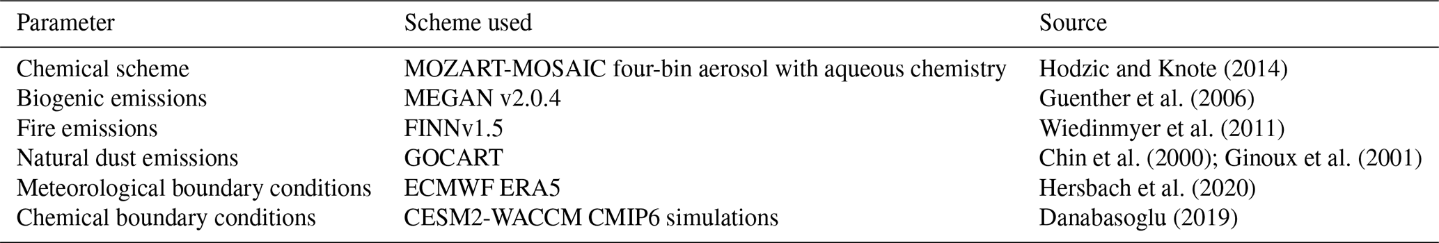

Table 1 Model parameters and sources used.

2014 was chosen as this is the most recent year of historical emissions data from the emissions inventory used in CMIP6. We also use CMIP6 output from CESM2-WACCM (Danabasoglu, 2019) simulations to provide initial and chemical boundary conditions. To simulate the chemistry, a scheme described by Hodzic and Knote (2014) is used that combines MOZART-4 gas-phase chemistry, which includes 85 gas-phase species, 157 gas-phase reactions and 39 photolysis reactions (this scheme and the included reactions are provided by Emmons et al., 2010) with the MOSAIC aerosol-chemistry scheme described initially by Zaveri et al. (2008). This provides detailed chemistry for a range of aerosol species, including nitrate from ammonium nitrate (NO₃), sulfate (SO₄), organic carbon (OC), black carbon (BC), ammonium from other sources (NH₄), sodium and chloride, all in four size bins up to 10 µm in diameter. The combined scheme described by Hodzic and Knote (2014) enhances these by including aqueous chemistry, improving the treatment of monoterpenes and hydrocarbons, and updating the mechanism for calculating secondary organic aerosols. In the model, PM_2.5 is the sum of the total dry aerosol mass in the three smallest size bins (up to 2.5 µm in diameter) of the above aerosol components and “other inorganics” (OIN), which largely consists of dust. The full range of model inputs are shown in Table 1.

2.2 Emissions associated with CMIP6

We simulated three different emissions scenarios. SSP1-2.6 represents a scenario with accelerated mitigation of greenhouse gases and sustainable societal development. SSP2-4.5 is a “middle of the road” scenario in which the trajectory of greenhouse gas mitigation does not accelerate or decelerate strongly and there are no great changes in the uptake of sustainable behaviours. SSP3-7.0 is a scenario in which regional rivalry hampers greenhouse gas mitigation and sustainable development. The assumptions for air pollutant controls mirror the trajectories of greenhouse gas emissions in each scenario, with some non-linearity or deviations in particular species to match the scenario narrative. These are explained by Rao et al. (2017); in summary, SSP1 assumes an acceleration of pollution control progress, SSP3 assumes a deceleration, and SSP2 assumes neither a notable acceleration nor deceleration from present-day controls. Figure 1 shows how the emissions of key species change in future scenarios compared to the present day, demonstrating how the narrative scenarios translate to emissions data. Here, the non-methane VOCs are grouped. We see that SSP1-2.6 has considerably lower emissions of all pollutant species compared to the present day. Compared to SSP1-2.6, SSP2-4.5 and SSP3-7.0 have lower reductions in emissions overall and notably differing trajectories for NH₃ emissions, which increase compared to the present in both scenarios. The NH₃ emissions increases are largest in rural regions, including most of France and Spain and northern Poland. Both scenarios have NH₃ emissions decreases in Paris, the Rhine-Ruhr region, and coastal parts of Spain and Italy. There are differences between SSP3-7.0 and SSP2-4.5 for CH₄ emissions, which are mitigated following SSP2-4.5 but worsen following SSP3-7.0, and for CO, which is heavily mitigated following SSP1-2.6 and SS2-4.5 but reduces only minimally following SSP3-7.0.

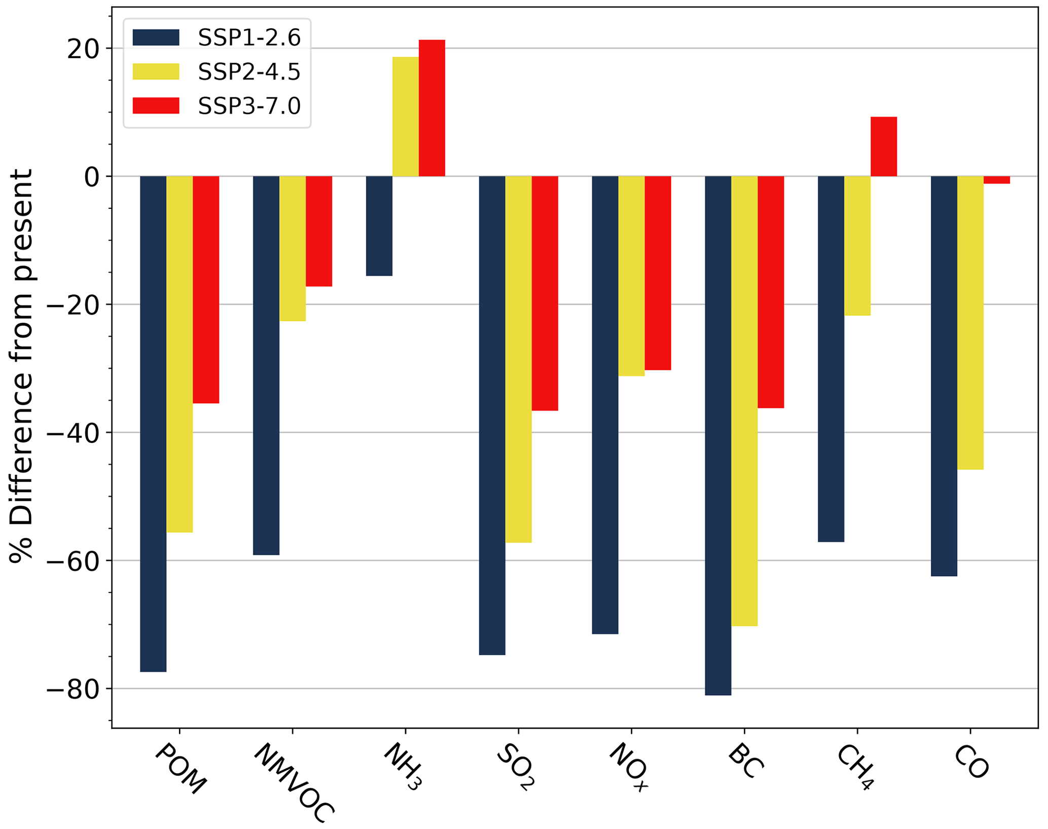
Figure 1 Relative change in model domain average annual emissions from 2014 to each of the future scenarios in 2050.

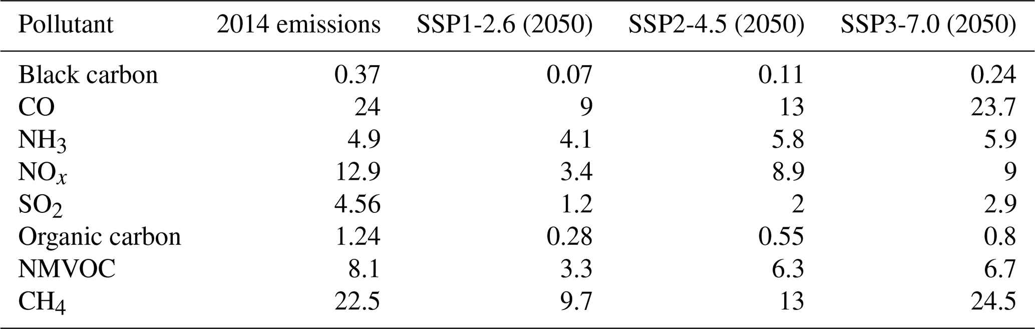
Table 2 shows the European total emissions of air pollutants assumed for the present-day scenario in 2014 and those in 2050 following the simulated scenarios, as taken from the input emissions files from Hoesly et al. (2018) for the present day and Feng et al. (2020) for the future scenarios. All the emissions files were at 50 km horizontal resolution. The emissions were then regridded to 30 km using a standard bilinear regridding method.

Table 2 European (the domain is defined in the main text) total emissions of air pollutants in 2014 from CMIP6 (Hoesly et al., 2018). and in 2050 from Scenario Model Intercomparison Project SSP1-2.6, SSP2-4.5 and SSP3-7.0 (Feng et al., 2020), all expressed in Mt yr⁻¹.

As the CMIP6 emissions do not include a component of inorganic PM_2.5 or PM₁₀ directly emitted as anthropogenic dust (as required for WRF-Chem), we created files to simulate this fraction as follows. We use linear regression to calculate the relationship between carbon monoxide and anthropogenic PM_2.5 and PM₁₀ in EDGAR-HTAPv2 (Janssens-Maenhout et al., 2015). We then apply this same relationship to the carbon monoxide emissions within CMIP6 to estimate emissions from anthropogenic PM_2.5 and PM₁₀. This methodology has been used previously by Kumar et al. (2018) and Wu et al. (2019). These input files are referred to in the rest of the text as anthropogenic dust emissions. To generate emissions of individual non-methane VOC (NMVOC) chemical species, we used scaling factors derived from ratios of individual NMVOCs to total NMVOCs in the EDGAR-HTAPv2 emissions inventory (Huang et al., 2017). This provided a greater spectrum of speciated VOCs than the scaling factors used by Hoesly et al. (2018) and Feng et al. (2020).

2.3 Model output

We use hourly output from each of the year-long WRF-Chem simulations for each species (O₃, CO, CH₄, SO₂, NO₂, nitrogen oxide (NO), NH₃, PM_2.5 dry aerosol mass and separate files for the individual PM_2.5 components, NO₃, NH₄, SO₄, OC, BC, sodium and chloride). All air pollutant output was analysed only at surface level. For some of the analysis, we weighted PM_2.5 and O₃ by population using the formula outlined in Abdul Shakor et al. (2020). We used time-varying gridded population projections for each SSP from Jones and O'Neill (2016). To represent the present-day population, the SSP2 population projection for 2020 was used. This was to allow for a consistent source of all population data as there were no data for 2014.

2.4 Model validation

The present-day simulation for 2014 was validated against PM_2.5, O₃ and other aerosol component observations (as detailed in Table 3) from the European Monitoring and Evaluation Programme (EMEP) as this features sites for a range of species across Europe. Sites with an altitude above 1 km were excluded as the measurement and modelling of air quality in complex terrain is challenging and frequently less accurate (Giovannini et al., 2020). We used spatial linear interpolation to extract data from our gridded model output to compare to the locations of the observation sites. The sites used are shown in Fig. A1.

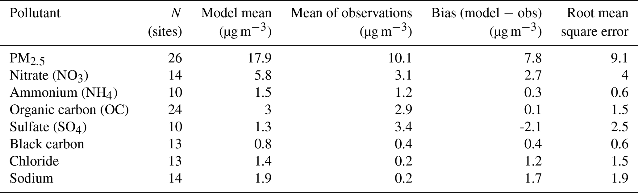
Table 3 Mean difference between annual mean model output and annual mean ground-based observations for different PM_2.5 components across monitoring sites in Europe.

Comparisons of modelled and observed O₃ and PM_2.5 are shown in Figs. 2 and 3. Figure 2 shows observed and simulated monthly mean PM_2.5 (a) and O₃ (b) colour coded by the observation station. Simulated monthly O₃ data show a slight underestimation (the mean absolute bias compared to observations was −3.40 µg m⁻³) overall. This underestimation is generally larger in the observation sites in Germany (Schmucke, Neuglobsow and Waldhof); however, an overestimation is seen in sites closer to the Mediterranean (Saint-Nazaire and Barcarrota). There were no available O₃ observations for Vredepeel, Cabauw Wielsekade, Guipry and Melpitz. PM_2.5 showed an overestimation compared to observations, with a mean absolute bias of 7.98 µg m⁻³. The sites with the largest overestimation were Cabauw Wielsekade, Harwell and Vredepeel. The overestimation was smaller in sites such as San Pablo de los Montes, Barcarrota and Penausende. The eastern European observation sites all showed a bias lower than the average. As all the observation sites use different monitoring technologies and all overestimate PM_2.5, we expect this to be an artefact of the model.

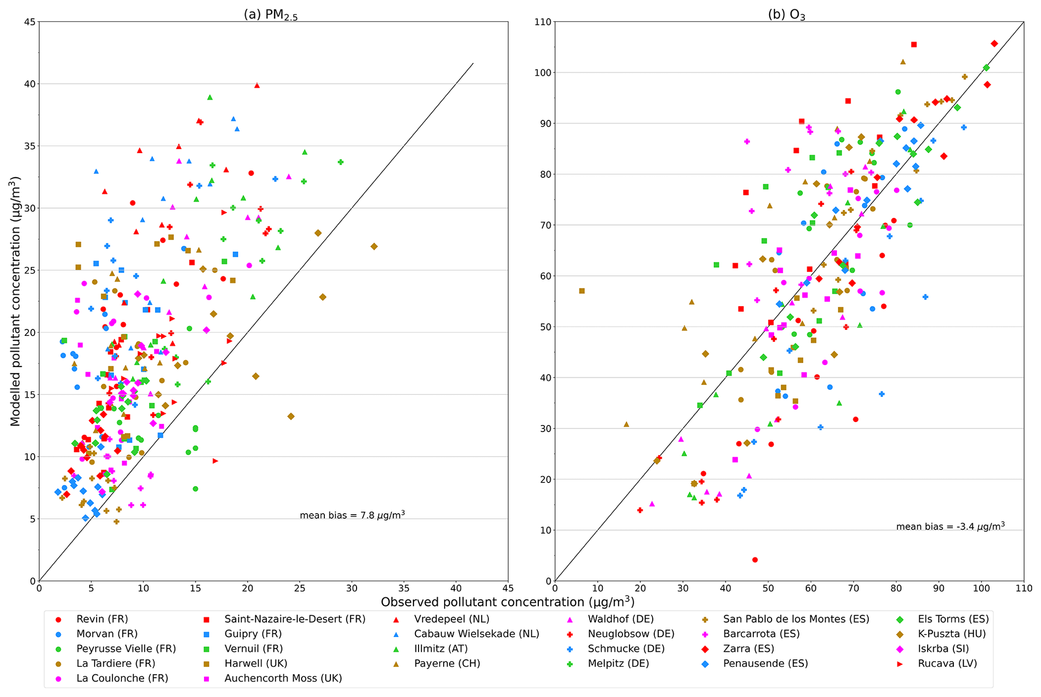
Figure 2 Comparison of modelled PM_2.5 (a) and O₃ (b) to ground-based observations. Monthly means are used for both species, and the units are µg m⁻³. Model data are interpolated from the latitude and longitude coordinates of the observation site. The middle line on each plot represents what the data would look like if the observations and model were equal.

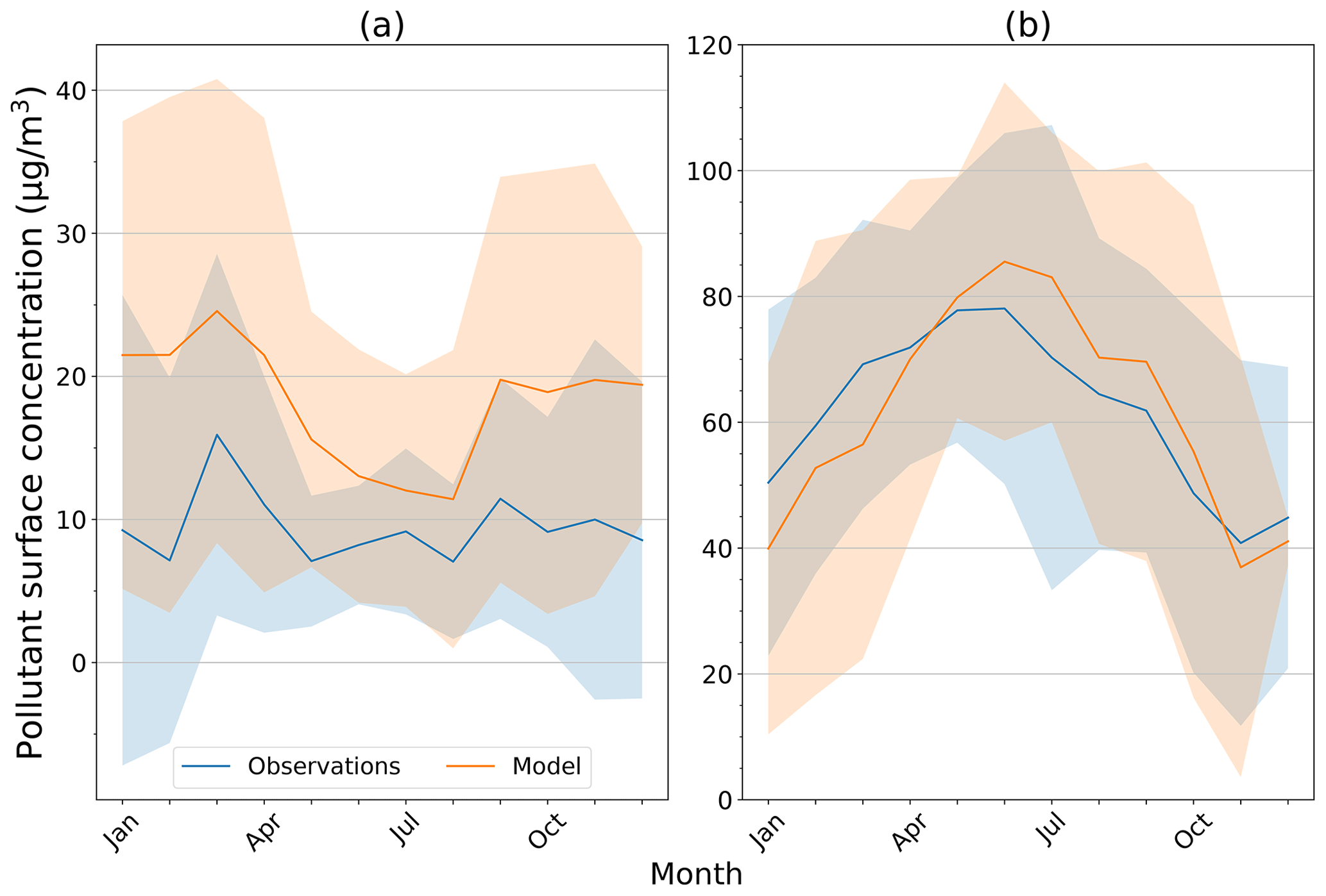
Figure 3 Seasonal cycles in 2014 of (a) PM_2.5 and (b) O₃: comparison of modelled monthly-mean data to observations (average of all sites). The number of sites is 26 for PM_2.5 and 21 for O₃. Both pollutants are measured in µg m⁻³. The shaded areas represent the variation from the mean across sites as 2 times the standard deviation.

Figure 3 is a comparison of modelled monthly-mean data with observations (averaged over all sites). The model presents a seasonal cycle, with higher PM_2.5 in spring and autumn, matching when the emissions peaked. The overestimation of PM_2.5 by the model was larger in spring and autumn and smaller in summer. The simulated O₃ showed seasonal biases: the model underestimated in winter and spring but overestimated during summer and autumn.

Turnock et al. (2020) reported an underestimation of PM_2.5 compared to observations in Europe in a similar period (2005–2014). This is likely because of the additional emission source of PM_2.5 in our simulations and the coarse resolution used by Turnock et al. (2020). Conversely, PM_2.5 overestimations have been seen in other studies that used CMIP6 emissions to drive regional models, such as Cheng et al. (2021), who found that nitrate, sulfate and ammonium PM_2.5 were overestimated by 30 %–60 % compared to observations when simulating over China.

Further validation of PM_2.5 components (a comparison of modelled values with ground-based observations) was conducted to diagnose the difference between the model and observations. This is shown in Table 3. The total bias in PM_2.5 is greater than the combined bias of the individual aerosol species. Although not every observation site measured each species and therefore the proportions cannot be assumed to be the same at each site, this implies that a different source may account for much of the bias. A large proportion of the bias likely comes from the OIN (dust) component. This agrees with previous research: Im et al. (2014) find that WRF-Chem setups using GOCART over-produce dust when the MOSAIC aerosol scheme is used. Similarly, when validating WRF-Chem over Cyprus, Georgiou et al. (2018) show that WRF-Chem simulations with MOSAIC aerosols can result in a significant overestimation of PM_2.5, largely driven by the dust scheme. Additionally, some of the overestimation in the OIN component is likely the result of the derived anthropogenic dust emissions as this is calculated from the CO emissions, which would explain the larger overall PM_2.5 overestimation in polluted urban regions.

Table 3 shows that the model overestimates NO₃ aerosol by 2.7 µg m⁻³ and underestimates SO₄ aerosol by −2.1 µg m⁻³ when compared to the observation sites. The overestimation of NO₃ aerosol matches the findings of other WRF-Chem studies, including Cheng et al. (2021) and Balzarini et al. (2015); however, both of these studies found an SO₄ overestimation as opposed to underestimation. The NO₃ overestimation may be the result of high NH₃ emissions over much of the year for the emissions used in CMIP6 in comparison to other emissions inventories. When compared to EDGAR-HTAPv3 (Crippa et al., 2023), CMIP6 NH₃ emissions were lower during February, March and April but higher for the rest of the year. Similarly, the CMIP6 emissions of nitrogen oxides (NO_x) are generally higher than EDGAR-HTAPv3 in urban regions, which may also contribute to the overestimation of NO₃ aerosols.

3 Results

3.1 Changes in PM_2.5

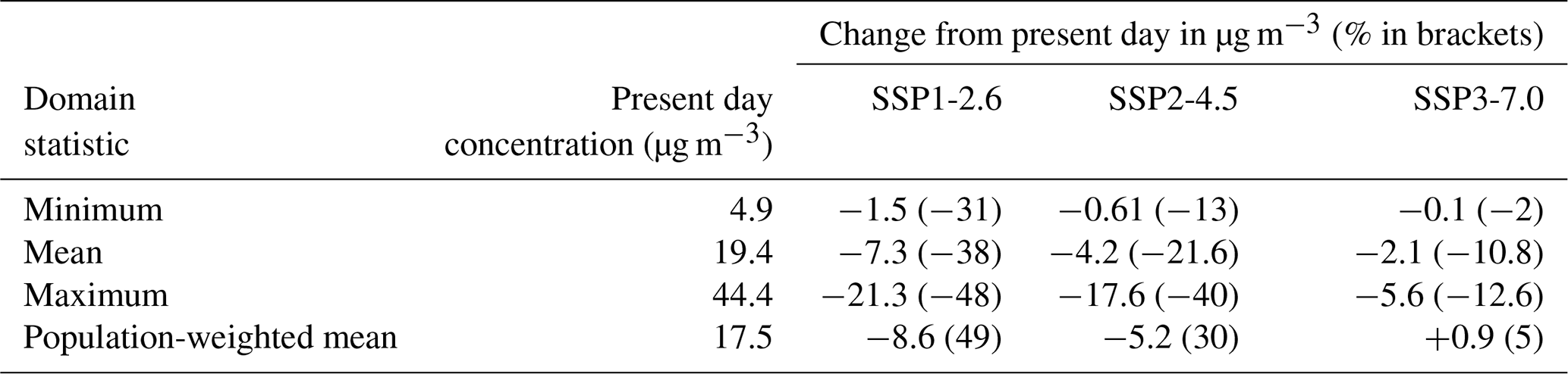
Table 4 shows the European annual mean PM_2.5 in the present day and the change from this in the future scenarios. In general, the annual mean PM_2.5 reduced in all future scenarios compared to the present day. The future reduction in European annual mean PM_2.5 of 38 % in SSP1-2.6 was far greater than the 11 % following SSP3-7.0. There are differences in the pattern when population weighting is applied; overall, population exposure to PM_2.5 increases slightly following SSP3-7.0 despite the domain-wide decrease. This suggests that the majority of the increases in PM_2.5 are in highly populated areas.

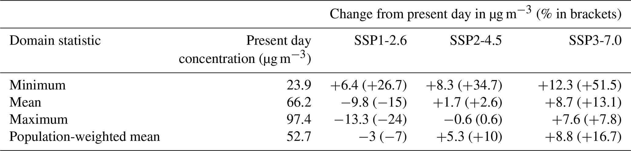
Table 4 Annual mean PM_2.5 whole-domain change statistics for each future scenario in 2050 compared to the present-day baseline (the left-hand column). For future scenarios, the raw change for each of these is shown in µg m⁻³, followed by the percentage change in brackets.

Spatially, we see greater reductions in PM_2.5 in urban and industrial regions than the domain average (Fig. 4 shows percentage changes between the present and future scenarios, while Fig. A2 shows the absolute changes). Both industrial (for example, the Po Valley in Northern Italy and the Rhine-Ruhr in north-western Germany) and urban regions see strong PM_2.5 reductions under SSP1-2.6 and SSP2-4.5 (although these are far larger following SSP1-2.6). Conversely, under SSP3-7.0, only urban regions see considerable PM_2.5 reductions. This could be explained by a larger reduction in industrial PM_2.5 emissions following SSP2-4.5 than SSP3-7.0 (−56 % compared to −47 %) and a larger reduction in OC emissions (−72 % compared to −65 %). Both SSP2-4.5 and SSP3-7.0 have small percentage increases in industrial NO_x and SO₂ emissions and relatively consistent NH₃ emissions when compared to the present day, suggesting that it is not differences in the NO_x and NH₃ ratio that cause the differences between SSP2-4.5 and SSP3-70 in industrial regions.

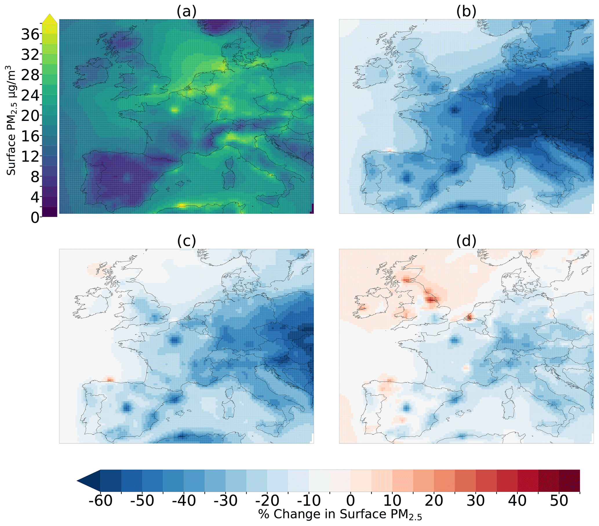
Figure 4 (a) Annual mean PM_2.5 (µg m⁻³) modelled using 2014 emissions. Panels (b), (c) and (d) show the annual mean PM_2.5 (µg m⁻³) simulated using 2050 emissions for SSP1-2.6, SSP2-4.5 and SSP3-7.0 respectively as the percentage change from (a).

Additionally, under SSP3-7.0, localised areas of worsening air quality are seen, including around East Yorkshire in the UK (worsening up to 4 µg m⁻³) and Zeeland and South Holland in the Netherlands (worsening up to 2 µg m⁻³). Some of these localised increases correspond with the locations of major combustion power plants, including Drax (North Yorkshire, UK) and Belchatow (central Poland). This is because the emissions scenarios assume that power generation emissions increase up to mid-century compared to the present day following SSP3-7.0; they drop following SSP2-4.5, but this is approximately half the reduction that is predicted following SSP1-2.6. All scenarios show slightly worsening PM_2.5 air quality of up to 2 µg m⁻³ near Gijon, on the northern coast of Spain. This reflects worsening NO_x emissions in all scenarios at this location.

The PM_2.5 reductions in SSP1-2.6 are larger across most of the domain compared to the other scenarios. This is most notable across central and eastern Europe (e.g. Germany, Poland, the Czech Republic and Austria). This is potentially because these regions have a larger proportion of anthropogenic PM_2.5 sources than natural sources. Smaller improvements are projected in countries such as Portugal and Ireland, where natural sources of PM_2.5 dominate. In the regions where the reductions in SSP1-2.6 compared to SSP2-4.5 and SSP3-7.0 are the largest (such as central and eastern Germany), the size of the reduction is likely the result of the combined reduction in NH₃ and NO_x emissions in SSP1-2.6 (−25 % and −70 %, respectively, domain-wide).

Across the domain, SSP2-4.5 and SSP3-7.0 have increases in NH₃ emissions (both approximately 20 %) and reductions in NO_x (both approx. −30 %) (Fig. 1). Where only NO_x is reduced, in some regions (usually NO_x-abundant regions), the increased oxidising capacity of the atmosphere can result in increased formation of secondary organic aerosol, thus limiting the efficacy of emissions reductions. This impact can be mitigated by joint reductions of both NO_x and NH₃ (Clappier et al., 2021). This is supported by the near-universal decreases of over 60 % in NO₃ PM_2.5 following SSP1-2.6, which are the result of a domain-wide reduction of 18 % of agricultural NO_x emissions and 7 % of agricultural NH₃ emissions. Following SSP2-4.5 and SSP3-7.0, NO₃ PM_2.5 does decrease universally; however, the reductions are much larger in urban than in rural regions. Notably, both of these scenarios have approximately 20 % increases in agricultural NH₃ emissions and increases in agricultural NO_x emissions (41 % following SSP2-4.5; 10 % following SSP3-7.0). This suggests that the difference in agricultural emissions will be a large driver of the extra reductions in PM_2.5 following SSP1-2.6, and the mitigation of emissions in this sector will be key to achieving improved air quality in Europe. It should, however, be noted that some rural regions (e.g. western France, Scotland, Wales and most of Spain) do still have overall NH₃ emissions increases following SSP1-2.6. This may explain the smaller reductions in PM_2.5 in these regions (Figs. A3 and A4).

Reductions in SO₂ emissions also contribute to the reduced PM_2.5. The countries that tend to see the largest decreases in PM_2.5 concentrations following the future scenarios are central/eastern European countries. These countries, particularly the urban areas of them, usually have a higher contribution from SO_x aerosol (including SO₄, which will cover much of this aerosol in the chemistry scheme) to PM_2.5 (Zauli-Sajani et al., 2024). SO_x aerosol is formed by reactions between SO₂, NO_x and NH₃. For example, atmospheric sulfuric acid is formed when SO₂ reacts with OH radicals. The sulfuric acid can then react with NH₃ to form SO₄ particulates (Clappier et al., 2021). Unlike for NH₃ and NO_x, there is limited non-linearity of SO₄ PM_2.5 reductions resulting from the mitigation of SO₂ emissions (Clappier et al., 2021). This means that SO₂ emissions reductions retain efficacy in reducing SO₄ PM_2.5 regardless of trends in NH₃ and NO_x emissions. SO₂ emissions reduce in all scenarios – by approximately 30 % for both SSP2-4.5 and SSP3-7.0 and by approximately 75 % following SSP1-2.6 (Fig. 1). This may explain why PM_2.5 reductions are most consistently seen in central and eastern Europe in all the future scenarios: in this region, reductions in SO₂ emissions (see Fig. A5) lower the PM_2.5 in the sulfate fraction to a greater degree than in western Europe. In western Europe, following SSP2-4.5 and SSP3-7.0, the reductions in NO_x in the absence of NH₃ hamper PM_2.5 reductions. This impact is reduced in eastern Europe, where NH₃ and NO_x provide a lesser contribution to PM_2.5 compared to SO₂, meaning that eastern Europe has larger PM_2.5 reductions following SSP2-4.5 and SSP3-7.0.

All countries show overall decreases in population-weighted PM_2.5 (Fig. 5). The magnitude of this varies greatly based on the scenario. Following SSP1-2.6, the percentage decrease ranges from 22.7 % in Ireland to 68.6 % in Hungary. Other countries with decreases in population-weighted mean PM_2.5 of greater than 50 % following SSP1-2.6 include Slovenia, Slovakia and Germany. These countries also see the greatest reductions in PM_2.5 following the other scenarios; for example, the largest reduction following SSP3-7.0 is in Slovenia, at nearly 25 %. This may be due to reductions in residential emissions, which see the greatest reduction as a proportion of total emissions in Slovenia and are reduced in all scenarios. This is in keeping with literature that identifies the importance of reducing residential-sector emissions to improve PM_2.5 concentrations in Europe, especially eastern Europe (Zauli-Sajani et al., 2024). For most countries in the domain, the agricultural sector contributes most to total air pollutant emissions.

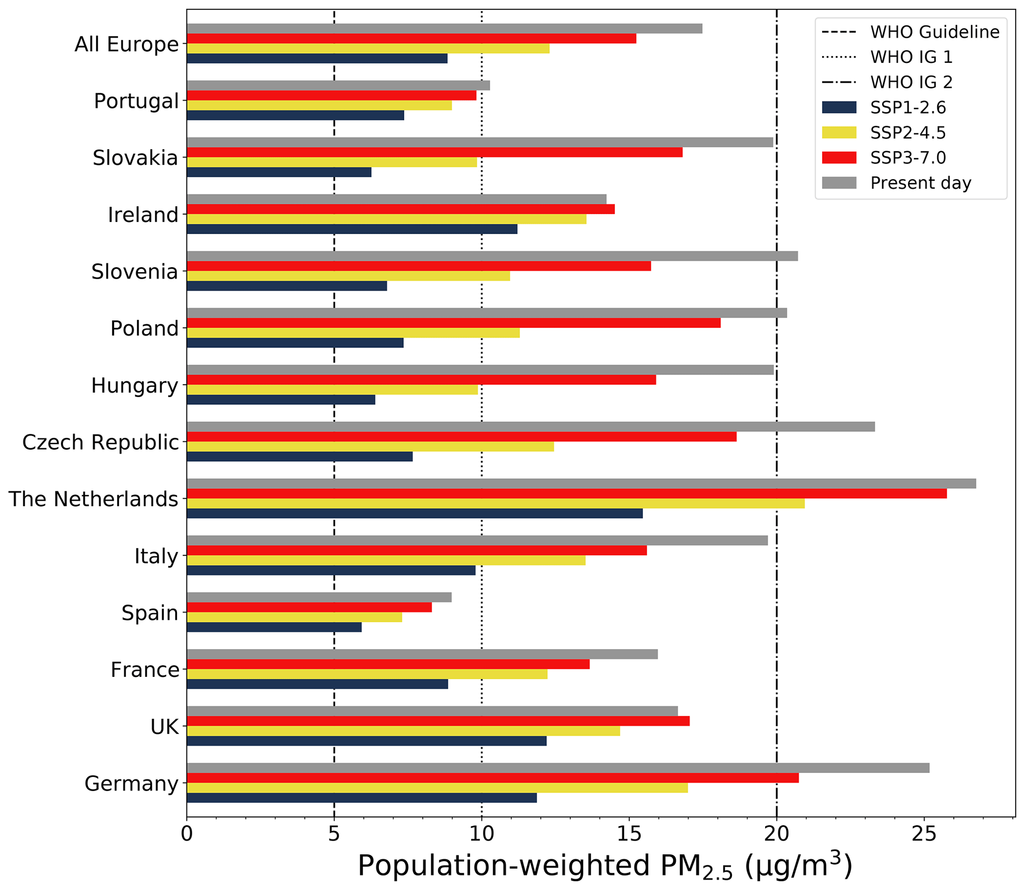
Figure 5 Population-weighted PM_2.5 in a selection of European countries following different scenarios compared to WHO guideline values. The lines labelled with “IG” are WHO interim guidelines. “All Europe” refers to a combined population-weighted mean of the 13 countries in the figure.

In addition to benefiting the least following SSP1-2.6, Ireland benefits the least following SSP2-4.5, with a reduction of 5 %. Similar to Ireland, Portugal and Spain do not benefit as much from the emissions changes compared to others. Ireland even shows an increase in population-weighted PM_2.5 following SSP3-7.0 of nearly 4 %, which is also seen in the UK. What this suggests is that the benefits are concentrated in countries where anthropogenic sources dominate PM_2.5 concentrations in the present day. As coastal-island countries, Ireland and the UK likely have a greater proportional quantity of natural sea salt aerosol making up PM_2.5 – previous literature suggests that sea salt PM_2.5 can reach up to 300 km inland and produce up to 5 µg m⁻³ of PM_2.5 (Manders et al., 2010). Spain and Portugal are likely to have large proportions of natural dust PM_2.5 due to their proximity to North Africa.

Figure 5 also compares the population-weighted mean to the World Health Organisation annual mean PM_2.5 guideline value of 5 µg m⁻³ (World Health Organisation, 2021). It suggests that following SSP1-2.6, many countries could see PM_2.5 exposure reduce below interim target values (guidelines the WHO suggest as targets to aim for before reaching the guideline value), representing a significant potential benefit for human health. Even the emissions reductions from SSP1-2.6 do not result in annual mean population-weighted PM_2.5 concentrations under this guideline, but when factoring in the average overestimation of PM_2.5 from our model, they are likely to be achievable in some locations. Notably, while countries where PM_2.5 is dominated by natural sources see less improvement, these have among the lowest PM_2.5 population exposure in the present day. This means that the benefits of the emissions changes are primarily seen in the countries that most need them. The whole-domain average also moves below the WHO interim target 1 of 10 µg m⁻³ following SSP1-2.6, after a reduction of almost 50 %.

Figure 6 shows the seasonal cycle of PM_2.5 components averaged across the entire model domain. SSP1-2.6 has a much lower contribution of anthropogenic PM_2.5 than SSP2-4.5 and SSP3-7.0, driven by the emissions reductions shown in Fig. 1. Figure 6 also shows that it is the change in these anthropogenic species, particularly in NO₃ and OC, that drive the differences between the future scenarios, with NO₃ alone reducing the total PM_2.5 following SSP1-2.6 by over 5 µg m⁻³ throughout much of the year. The importance of NO₃ aerosol in the future scenarios to determining the total PM_2.5 implies that NH₃ and NO_x emissions reductions will be key to improving future air quality. All future scenarios show overall reductions in NO_x emissions, which can limit the formation of NO₃ and NH₄ particulates (Pusede et al., 2016); however, it is only SSP1-2.6 that shows a significant reduction in NO₃ aerosol, likely because it is the only scenario where NH₃ emissions reduce compared to the present day. This suggests that agriculture will be a key sector for attaining air quality co-benefits as agriculture is a major source of NH₃ emissions. The reduction in OC concentrations is proportionally far larger under SSP1-2.6 than the other scenarios, potentially due to the trajectories of power sector OC emissions.

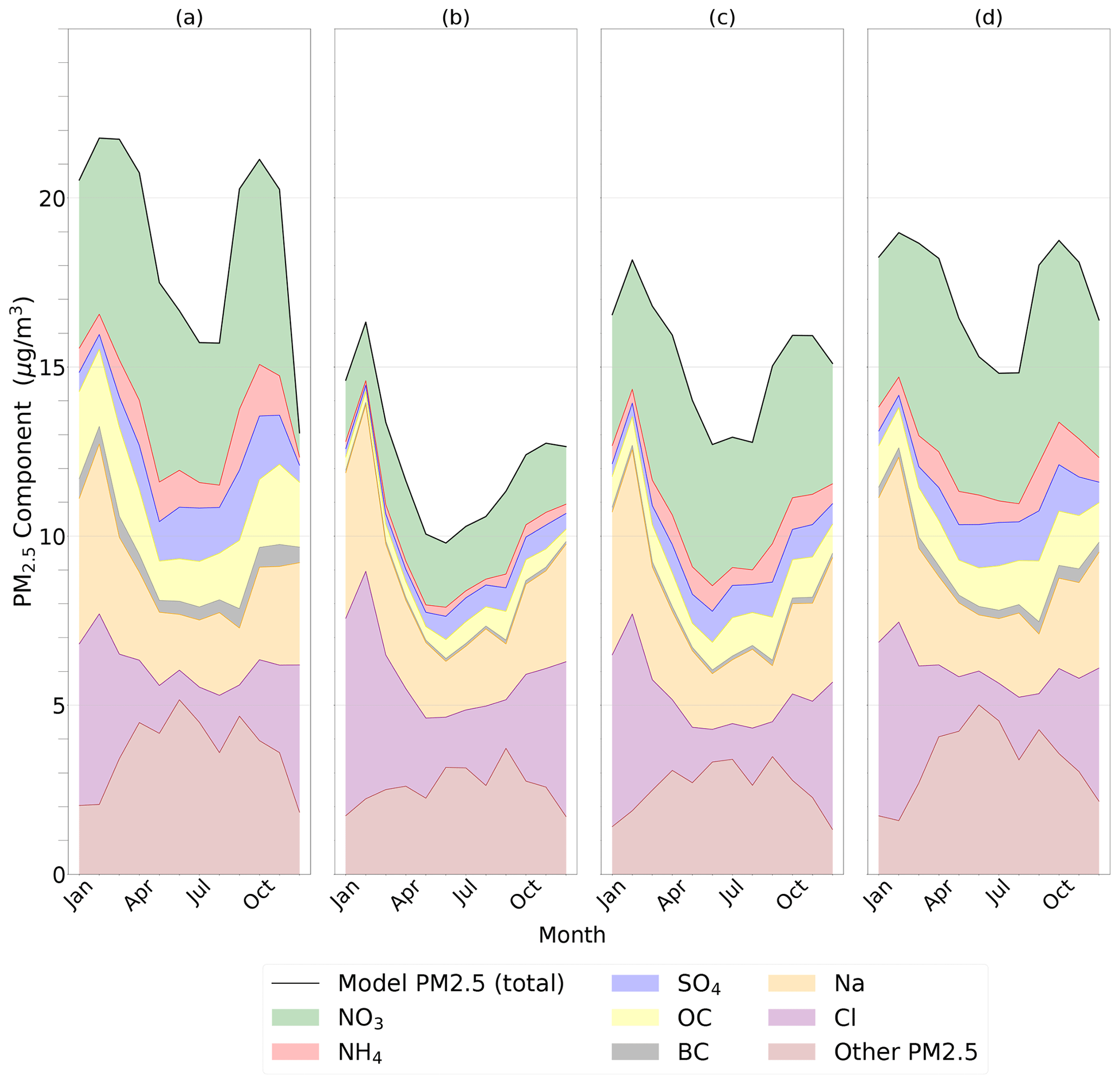
Figure 6 Seasonal cycle of domain-average PM_2.5 over each simulation by component. Panel (a) shows the results from the 2014 simulation, while (b), (c) and (d) show the results for 2050 from each of SSP1-2.6, SSP2-4.5 and SSP3-7.0 respectively.

Our findings are in agreement with other work in the area in that we find that air quality co-benefits of climate mitigation are likely for PM_2.5. When compared to Fenech et al. (2021) (who used CMIP5 emissions and focused on the UK) for example, we see that both studies project that strong mitigation will result in air quality co-benefits in terms of PM_2.5 for the UK. The reductions we project for the most comparable scenarios (SSP1-2.6 and RCP2.6) are larger (−7.3 as opposed to −2.2 µg m⁻³ or approximately 38 % vs 25 %). We see a diverging trend for the most pessimistic scenarios – while they see reductions in PM_2.5 concentrations following RCP8.5, we see worsening PM_2.5 following SSP3-7.0.

Notably, our model simulated high present-day PM_2.5 in urban regions (e.g. Paris, Madrid and London) compared to surrounding areas. It also produced elevated PM_2.5 in heavily industrial regions of Europe such as the Po Valley and the Rhine-Ruhr (Fig. 4a). It is the changes in these regions that stand out in the other panels of Fig. 4. What this suggests is that our methodology allows us to better represent changes on a local level than work using climate model output. This can be shown when our work is compared to Turnock et al. (2020) (who used CMIP6 output for a global domain) in Fig. 7, which shows the difference in the change between the present and 2050 following SSP3-7.0 for both PM_2.5 and O₃. Figure 7 shows that we see similar spatial changes except for different trends in PM_2.5 across the Iberian Peninsula and most of the British Isles. This comparison shows how the finer spatial resolution allows us to see localised elevated concentrations of pollution, whereas pollutants are distributed more evenly over the coarser resolution of global models. We also see greater improvements in PM_2.5 overall than Turnock et al. (2020); for example, for SSP1-2.6, our domain improvement of 7 µg m⁻³ is more than double theirs (approximately 3 µg m⁻³). This highlights that using air pollutant concentrations from global model simulations may underestimate the extent of future changes in air quality.

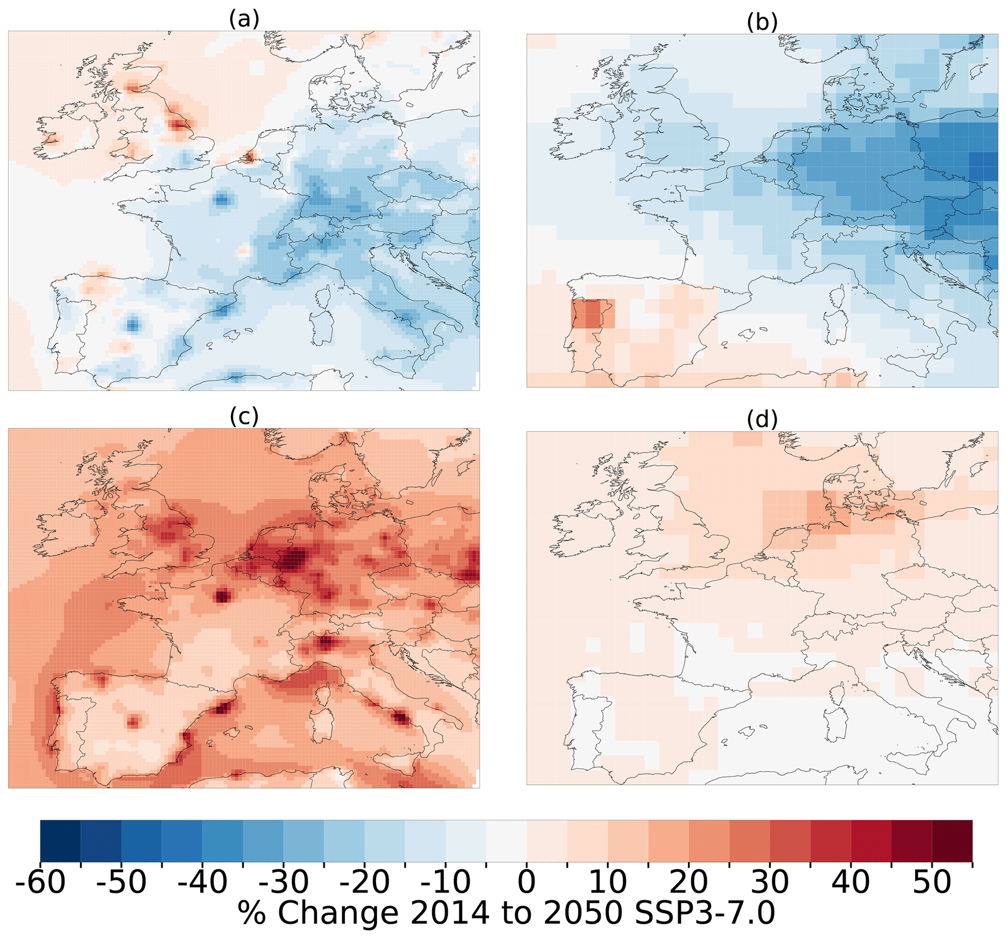
Figure 7 Percentage change in annual mean PM_2.5 between the present day and 2050 following SSP3-7.0 (a) from our simulations with WRF-Chem and (b) from Turnock et al. (2020), who used CMIP6 multi-model output. (c, d) As (a, b) but with O₃ compared; note that the annual mean O₃ is considered here, so (c) differs from panel (d) of Fig. 10.

Geographically, the reductions in European PM_2.5 are lower than those in more polluted regions in other studies. Cheng et al. (2021) find a reduction in population-weighted mean PM_2.5 in China between 2020 and 2050 following SSP1-2.6 of between 20 and 25 µg m⁻³ (from approximately 42 µg m⁻³ in the present-day scenario). However, this reduction is similar to the average relative reduction of 52 % across European countries that we find. Studies on future air quality in India also find that scenarios with a greater focus on sustainability result in reductions in surface air pollution (Chowdhury et al., 2018; Kumar et al., 2018), although methodological differences make direct comparisons with these studies challenging. What these comparisons suggest is that Europe could see similar relative air quality co-benefits to other regions following future sustainability scenarios.

3.2 Changes in O₃

The maximum 6-monthly-mean daily-maximum 8 h (6mDM8h) O₃ shows marginally higher concentrations in Mediterranean regions, including Italy, southern Spain and the French Riviera, which get more sunlight (Fig. 8 shows percentage changes between the present and future simulations, while Fig. A6 shows the absolute changes). In the simulations using future scenarios, O₃ strongly reduces following SSP1-2.6 (a mean reduction of approximately 15 %), whereas SSP2-4.5 shows variation across the domain. While the mean change is a reduction of approximately 3 %, increases are seen in most of England, the Benelux region and north-western Germany. 6mDM8h O₃ increases across most of the domain following SSP3-7.0 (a mean increase of approximately 13 %). This is not universal; small decreases of up to 5 % are seen in most of the Mediterranean regions with high present-day O₃. Despite the lack of peaks in the present-day simulation, in the future simulations, O₃ pollution does not reduce as much in urban regions as it does in much of the rest of the domain following SSP1-2.6. The same regions show increases following SSP2-4.5 (and some regions, such those as around Barcelona and Naples, show increases following SSP1-2.6), whereas much of the rest of the domain has reductions in surface level O₃, and the increases are higher than in surrounding areas following SSP3-7.0.

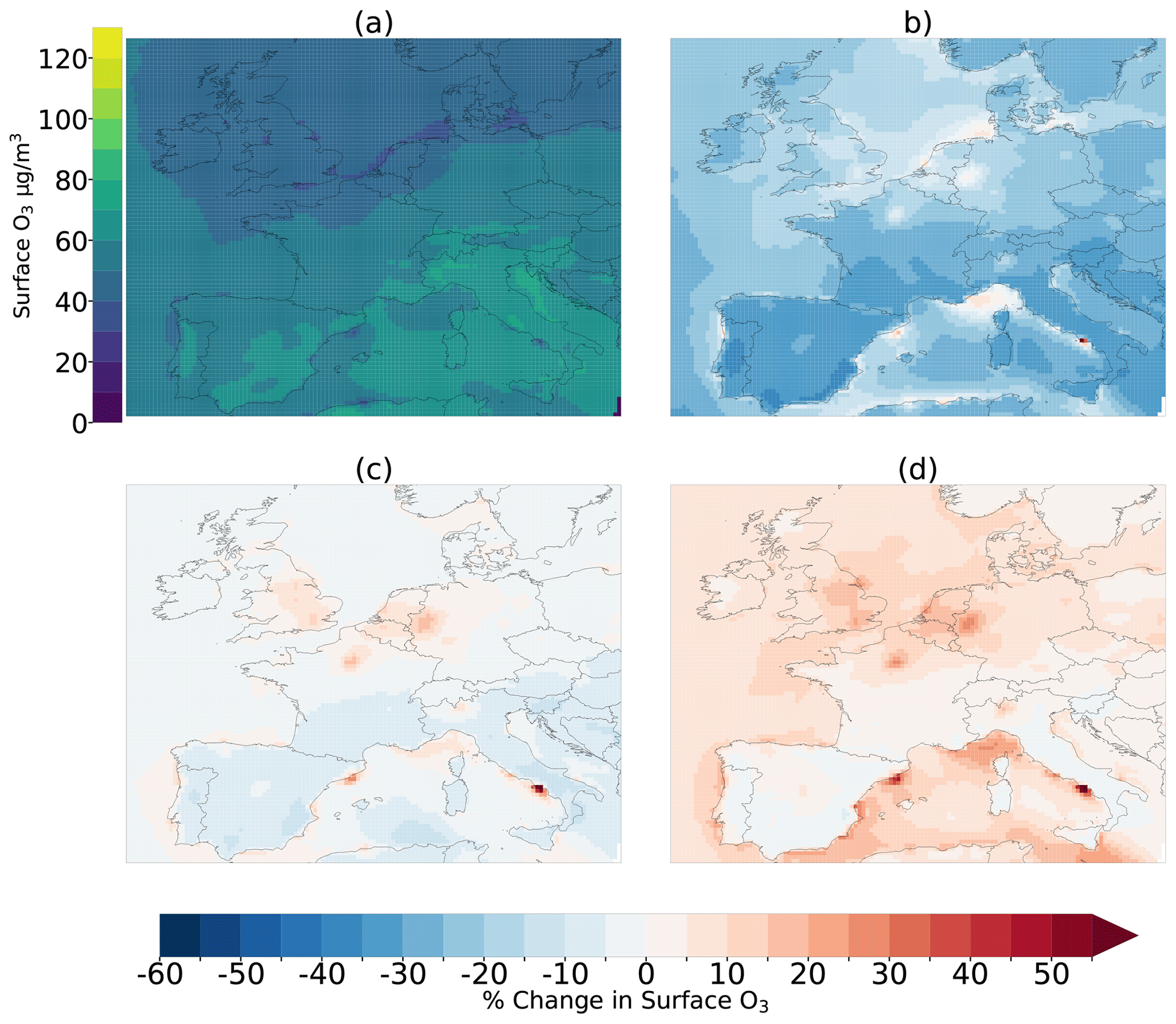
Figure 8 6mDM8h O₃ calculated as the highest 6-month mean of the highest rolling 8 h O₃ in 24 h periods in the O₃ output for each scenario. Panel (a) shows this metric for the CMIP6 2014 simulation. Panels (b), (c) and (d) show the percentage changes from this for SSP1-2.6, SSP2-4.5 and SSP3-7.0 respectively.

Table 5 Annual mean O₃ whole-domain change statistics for each future scenario compared to the present-day baseline (the left-hand column). For future scenarios, the absolute change for each of these is shown in µg m⁻³, followed by the percentage change in brackets.

The differing trends in CH₄, CO and NO_x (Fig. 1) between the scenarios may explain the difference in O₃. It is well established in the literature that in urban areas, reductions in NO_x emissions can cause increases in surface-level O₃, including within Europe (Lee et al., 2020; Finch and Palmer, 2020). This is due to increased titration of O₃, in which reduced NO concentrations due to the reductions in NO_x emissions result in less destruction of O₃ molecules (Monks et al., 2015). This is supported by our results, as the largest O₃ increases are seen in the urban areas with the largest reductions in NO₂, such as Naples (Italy) and Barcelona (Spain) (Fig. A7). This effect is likely to be amplified in autumn and winter, when emissions reduction policies are likely to have the most impact. Figures A9–A12 support this, showing that the O₃ increases are largest during the winter months. This is why the annual mean O₃ concentration changes (Fig. A8) follow a different pattern to 6mDM8h O₃.

Reductions in NMVOCs could be having similar effects to the NO_x reductions in some regions. In all scenarios, reductions in NO_x emissions are stronger than NMVOC emissions; however, following SSP2-4.5 and SSP3-7.0, the proportional gap is much larger. This suggests that in VOC-limited regimes (which are generally urban areas), where reductions in NO_x are more likely to exacerbate O₃, we may see a larger O₃ response. Notably, the emissions changes may cause different patterns in NO_x and VOC-limited regimes that may impact on the O₃ response; for example, Liu et al. (2022) find that in Europe following SSP3-7.0, the percentage of VOC-limited areas drops from nearly 80 % to 27 % in winter and from 37 % to under 3 % in summer. If our simulations have a similar change in sensitivity, this could suggest that a different precursor, such as CH₄, primarily drives the increases in O₃ following SSP3-70, which suggests that agriculture will be a key sector for determining future O₃ pollution.

In SSP1-2.6, this impact of reduced NO_x emissions causing O₃ increases is masked by O₃ increases from another source, likely much stronger decreases in CO and CH₄ emissions than in SSP2-4.5 and SSP3-7.0. What this means is that while all scenarios assume increased pollution control, the additional focus given to climate mitigation (e.g. reducing CH₄ emissions) and the more sustainable socioeconomic development in SSP1-2.6 and SSP2-4.5 have potential air quality co-benefits by outweighing any impacts on O₃ from reduced NO_x. O₃ is considerably more impactful on health during the peak season due to the high thresholds needed to affect population health on a large scale, so most parts of Europe will see a reduced impact of O₃ pollution following both SSP1-2.6 and SSP2-4.5.

We find a considerably higher percentage increase in annual mean O₃ in 2050 following SSP3-7.0 compared to that found for Europe by Turnock et al. (2020) (Fig. 7). Once again, the difference in resolution is clear here, as we see much larger increases in O₃ around certain urban regions, whereas Turnock et al. (2020) show a smaller trend distributed over larger areas. As with PM_2.5, the finer resolution we use could prove valuable, especially for understanding health impacts and trends in urban areas. As shown by the contrasting trends in urban and rural areas for O₃ pollution following some scenarios, being able to represent these changes is valuable.

Compared to studies focusing on regions outside of Europe, our findings are similar to those reported by Zhang et al. (2017), who use WRF-Chem to simulate the impact of RCPs on air pollutants over the USA. They find overall small decreases in 6mDM8h O₃ (up to 2 ppb) except in some large urban areas following RCP4.5, where they report increases of up to 10 ppb. Following SSP2-4.5, we see a similar trend (an average reduction of −1.5 ppb but localised increases around some cities and industrialised areas).

4 Limitations

There are limitations of this study to be considered. Primary among these is the overestimation of PM_2.5 concentrations in the present day. While these are mostly systemic, they should be taken into account when considering the absolute concentrations reported, especially when compared to air quality guideline values. It is likely that the percentage changes we see would be less drastic had the model not overestimated PM_2.5. As the model overestimates NO₃ and underestimates SO₄ PM_2.5, we may overestimate the impacts on changes in NH₃ and NO_x emissions on future air quality, particularly in the agricultural sector compared to other sectors such as industry.

The resolution that we use is designed for the region or country scale and not the urban scale. A horizontal resolution of 30 km is unlikely to faithfully capture atmospheric chemistry at the city scale. Although we can represent the locations of urban and industrial peaks, be aware that the model may not simulate chemistry at this scale as effectively as a finer-scale model.

We also do not control for the impacts of population change in the future scenarios in Table 4, Fig. 6 or Table 5.

5 Summary and conclusions

We use emissions data for three SSPs (SSP1-2.6, SSP2-4.5 and SSP3-7.0), representing very different climate futures, to simulate air quality in Europe in 2050 compared to the present day. This work uses WRF-Chem v4.2, with a much more detailed chemistry scheme and finer grid resolution than much of the previous work using SSPs, to provide a more detailed assessment of potential air quality co-benefits on a regional scale.

We show that while PM_2.5 is expected to reduce compared to the present day across most of Europe in all future scenarios, it shows by far the biggest reductions in scenarios with a greater focus on sustainability and therefore more stringent emissions reductions. We find that in 2050, following SSP1-2.6, mean population-weighted PM_2.5 concentrations across European countries reduce by 52 % compared to 2014. Under SSP2-4.5, this average reduction is 34 %. The smallest average reduction was 18 %, obtained following SSP3-7.0. The additional benefits we see following SSP1-2.6 are likely due to emissions reductions in the agricultural and industrial sectors.

We also show the sign of O₃ change differs across the scenarios: in the more sustainable scenario, SSP1-2.6 (and, to a lesser extent, SSP2-4.5), much of Europe will see reduced 6mDM8h O₃ concentrations, whereas 6mDM8h O₃ will worsen following SSP3-7.0. This is likely driven by a combination of reduced NO_x and increased CH₄ emissions. This demonstrates the importance of reducing CH₄ alongside other O₃ precursor species to avoid reducing the efficacy of overall air pollutant controls, which is caused by focusing entirely on PM_2.5 and NO_x without also considering the impacts on O₃, as is evident from the increases in O₃ concentrations during the COVID-19 lockdowns, where large reductions in NO_x emissions occurred with a smaller or no effect on CH₄ (Jephcote et al., 2021; Miyazaki et al., 2021).

We find that using a regional atmospheric-chemistry model provides us with the ability to analyse in more detail where air quality in Europe could change in response to the scenarios and that the patterns in air quality changes obtained using this methodology differ from what you get using climate model output. From that, we can make a more informed hypothesis as to why air pollutants respond the way they do, based on sector-specific emissions changes. We demonstrate the value that can be added by using this methodology; for example, it can provide country-specific population-weighted mean changes, which may be more useful to regional and national policymakers. This demonstrates the importance of a combined approach to modelling air quality co-benefits using both global and regional models.

To conclude, our results suggest that air quality co-benefits will be seen if society follows a pathway in which environmental sustainability is a priority, particularly in terms of mitigating climate change. This implies there are potential public-health benefits, although the results of this may differ from those of other studies, so further studies to calculate the health benefits are important.

Appendix A: Appendix figures

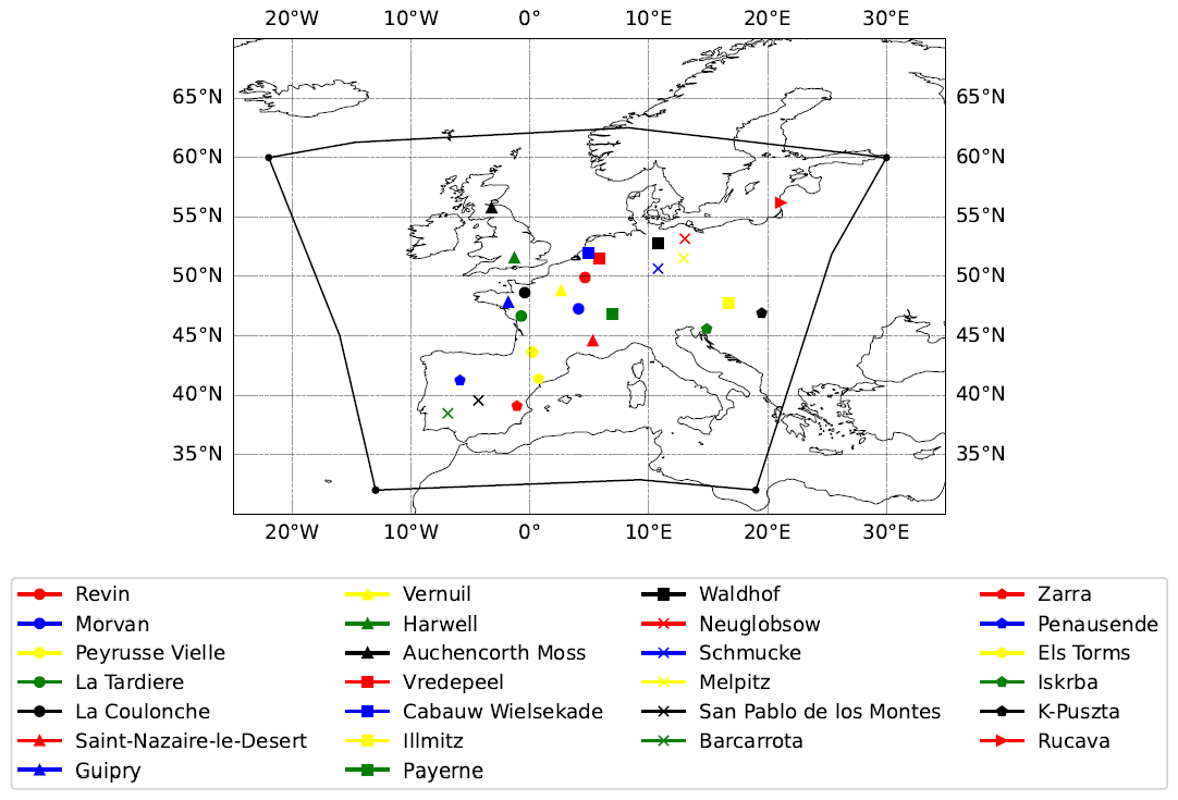
Figure A1 The domain input into WRF-Chem v4.2 for our simulations at 30 km resolution. The observation sites used for model validation are also shown.

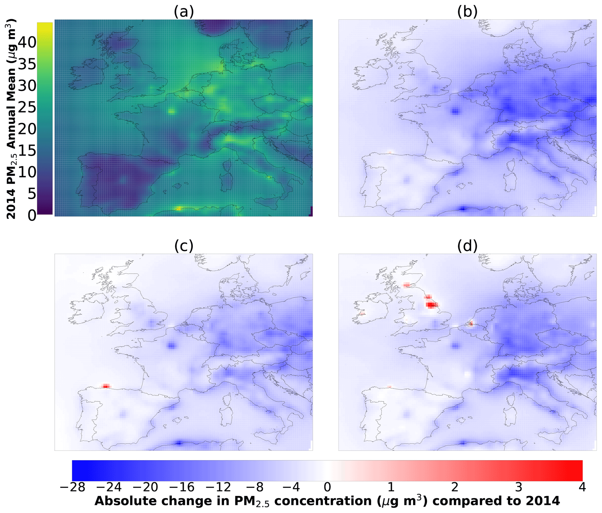
Figure A2 Annual mean PM_2.5 for each scenario. Panel (a) shows this metric for the CMIP6 2014 simulation. Panels (b), (c) and (d) show the absolute change from this for SSP1-2.6, SSP2-4.5 and SSP3-7.0 respectively.

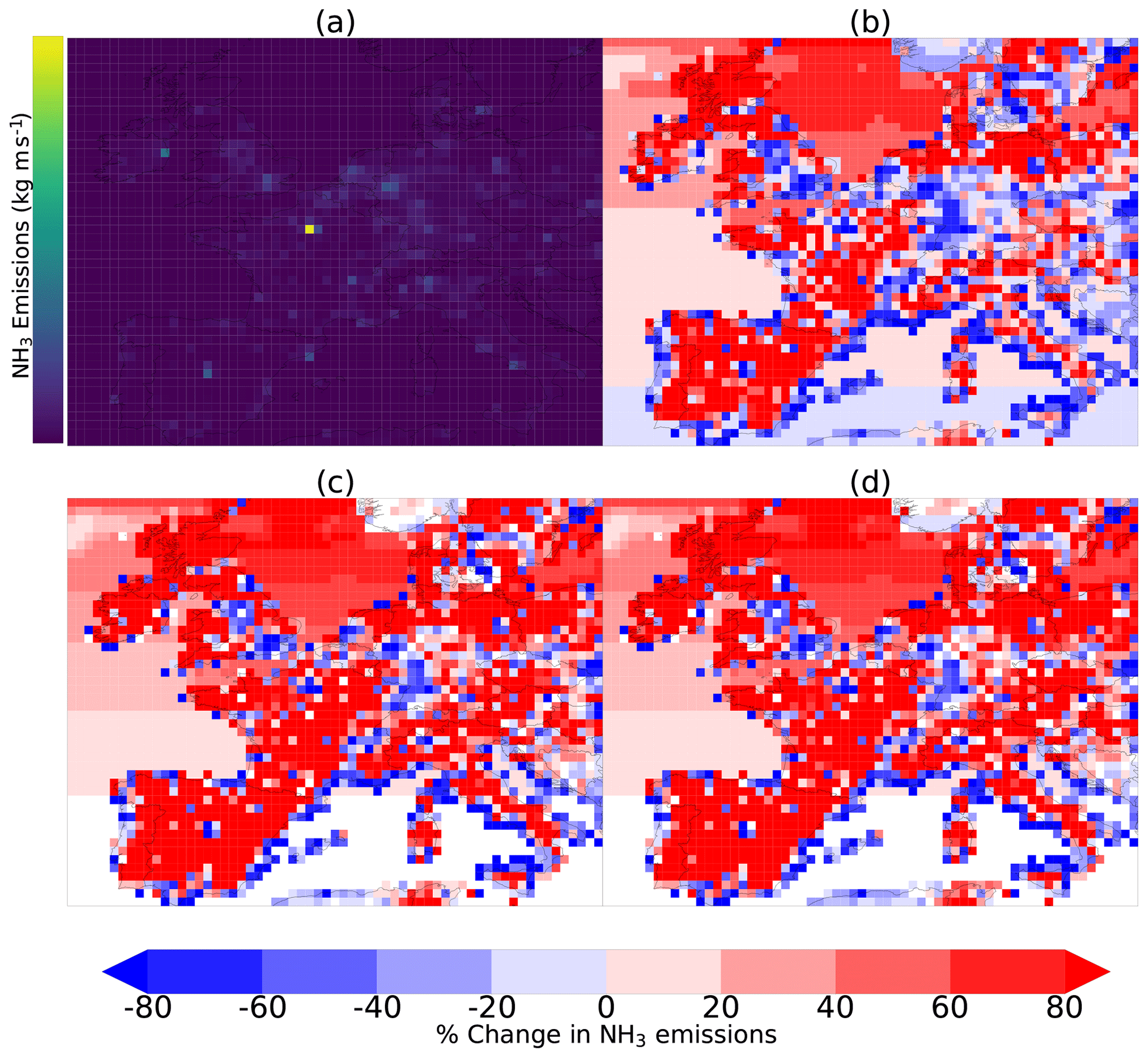
Figure A3 Annual mean NH₃ emissions for each scenario. Panel (a) shows this metric for 2014. Panels (b), (c) and (d) show the percentage change from this for SSP1-2.6, SSP2-4.5 and SSP3-7.0 in 2050 respectively.

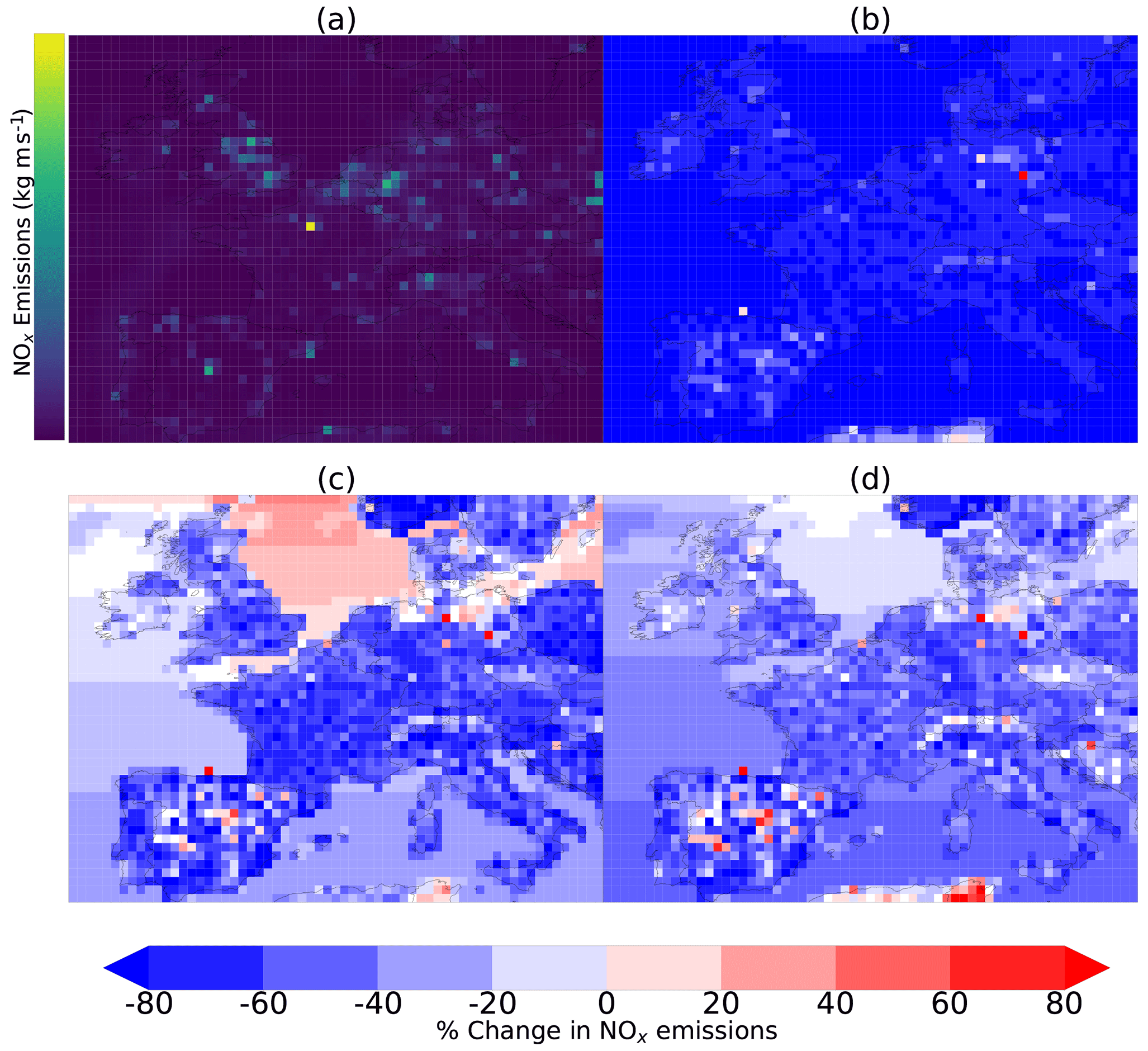
Figure A4 Annual mean NO_x emissions for each scenario. Panel (a) shows this metric for 2014. Panels (b), (c) and (d) show the percentage change from this for SSP1-2.6, SSP2-4.5 and SSP3-7.0 in 2050 respectively.

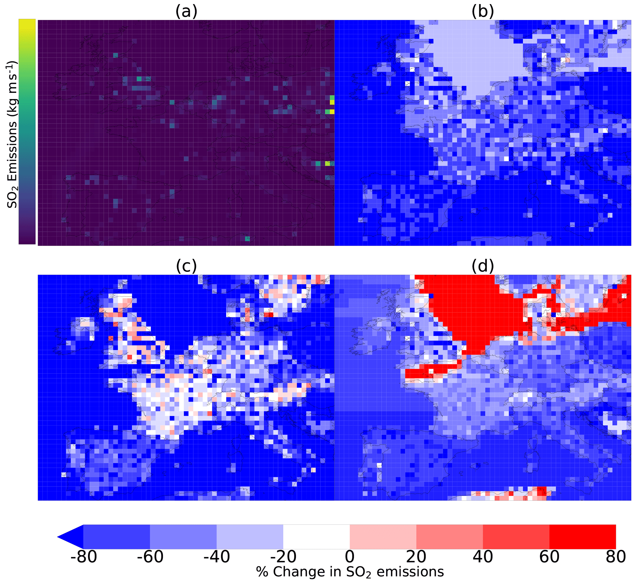
Figure A5 Annual mean SO₂ emissions for each scenario. Panel (a) shows this metric for 2014. Panels (b), (c) and (d) show the percentage change from this for SSP1-2.6, SSP2-4.5 and SSP3-7.0 in 2050 respectively.

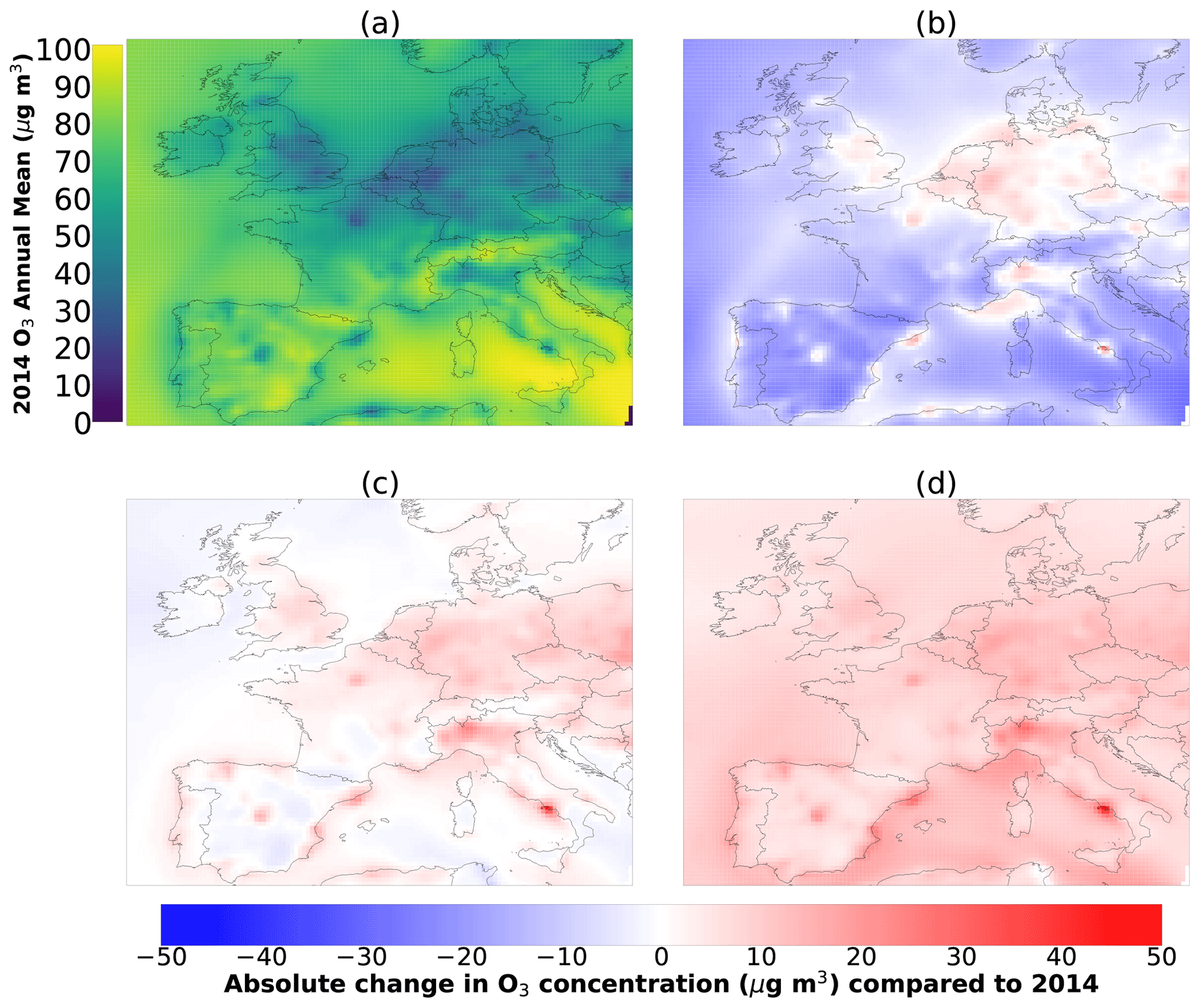
Figure A6 6mDM8h O₃ for each scenario. Panel (a) shows this metric for the CMIP6 2014 simulation. Panels (b), (c) and (d) show the absolute change from this for SSP1-2.6, SSP2-4.5 and SSP3-7.0 respectively.

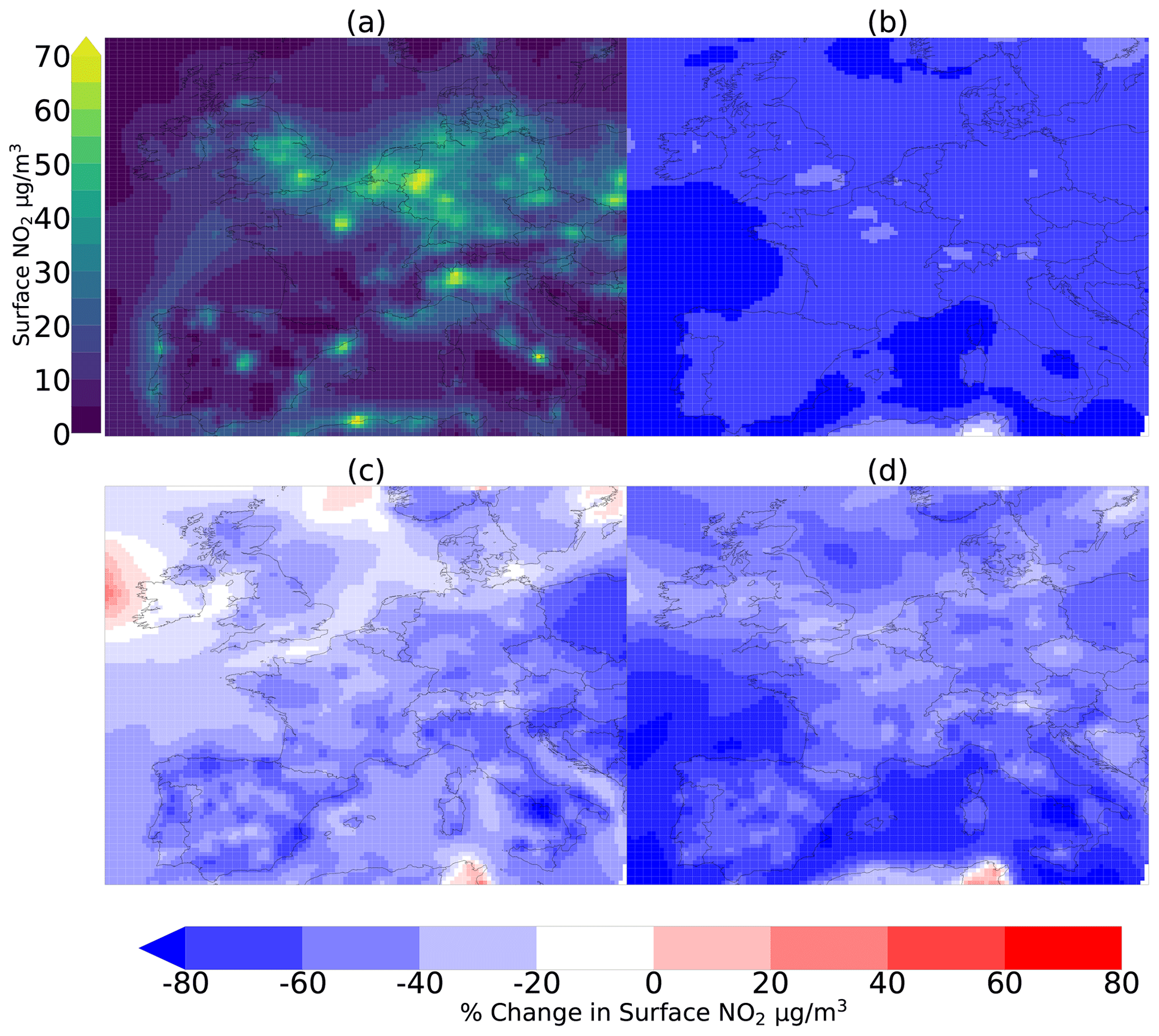
Figure A7 Annual mean NO₂ for each scenario. Panel (a) shows this metric for the CMIP6 2014 simulation. Panels (b), (c) and (d) show the percentage change from this for SSP1-2.6, SSP2-4.5 and SSP3-7.0 respectively.

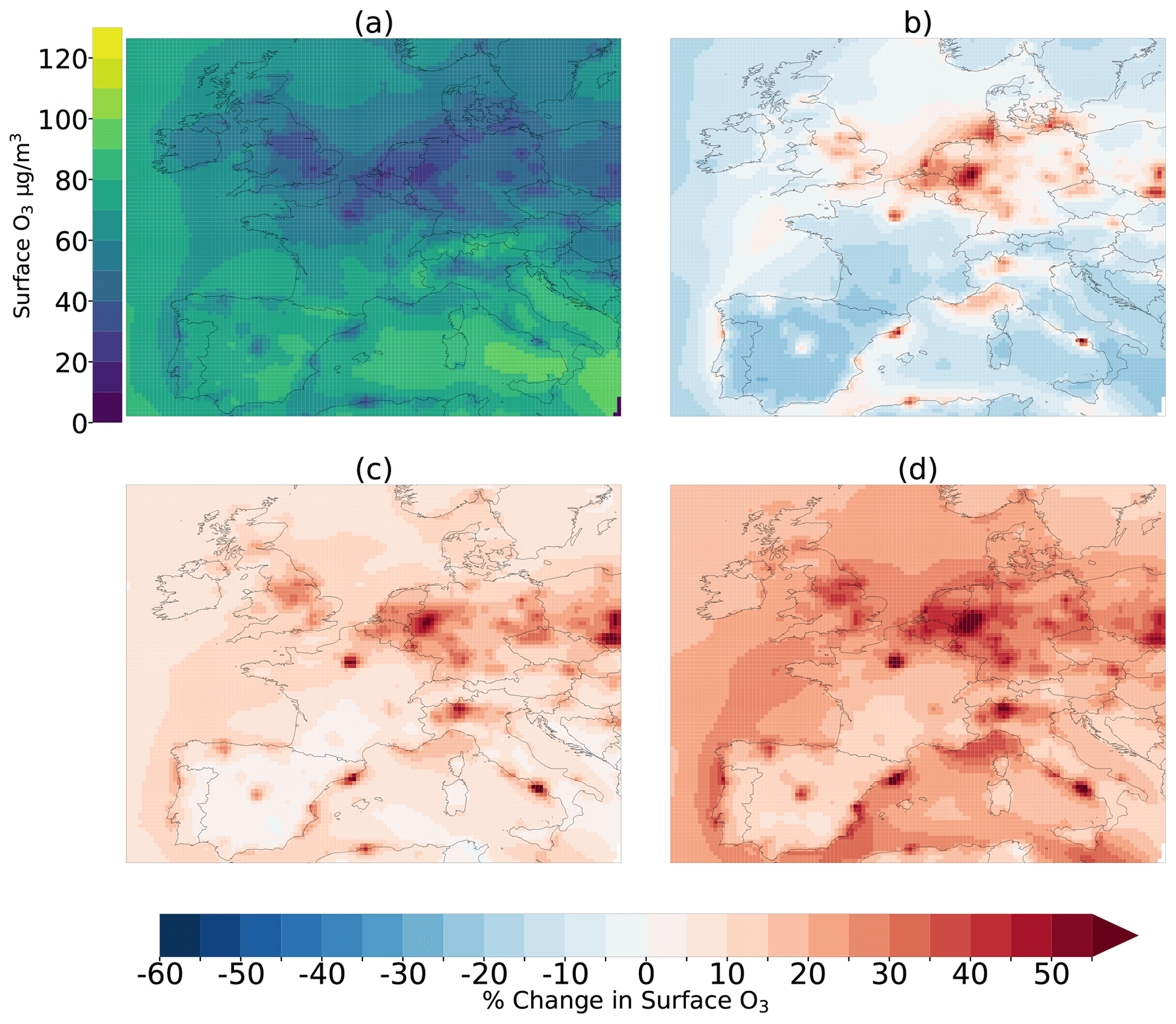
Figure A8 Annual mean O₃ for each scenario. Panel (a) shows this metric for the CMIP6 2014 simulation. Panels (b), (c) and (d) show the percentage change from this for SSP1-2.6, SSP2-4.5 and SSP3-7.0 respectively.

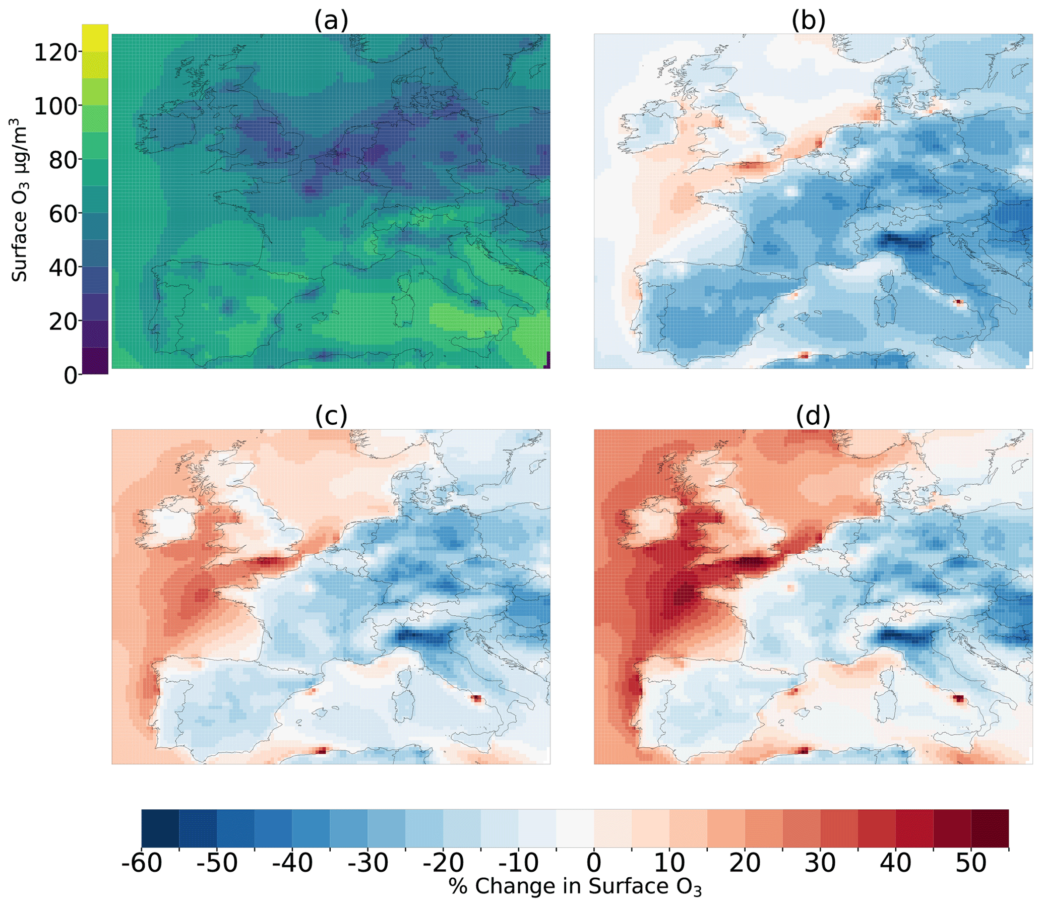
Figure A9 Mean O₃ in January, February and December for each scenario. Panel (a) shows this metric for the CMIP6 2014 simulation. Panels (b), (c) and (d) show the percentage change from this for SSP1-2.6, SSP2-4.5 and SSP3-7.0 respectively.

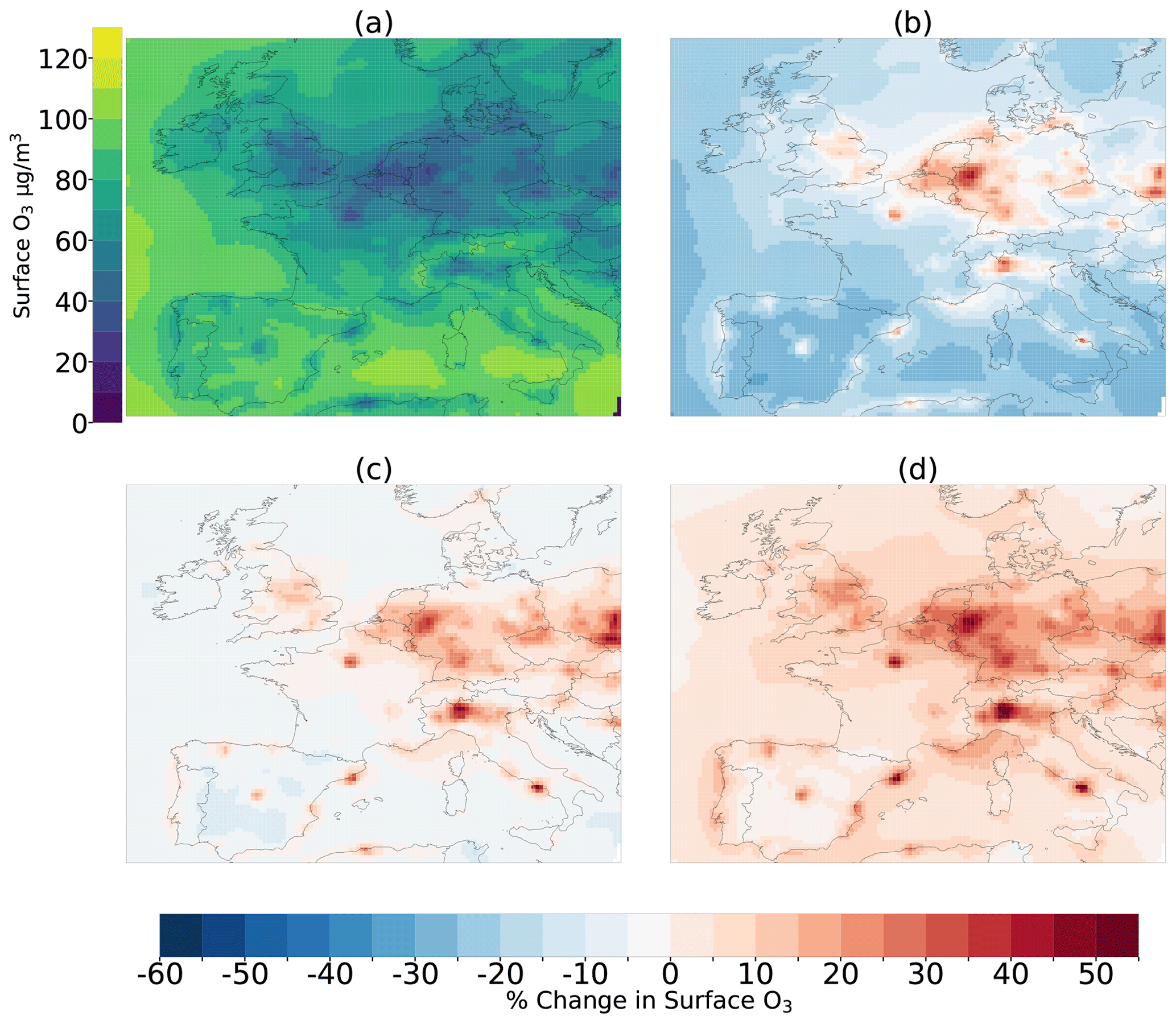
Figure A10 Mean O₃ in March, April and May for each scenario. Panel (a) shows this metric for the CMIP6 2014 simulation. Panels (b), (c) and (d) show the percentage change from this for SSP1-2.6, SSP2-4.5 and SSP3-7.0 respectively.

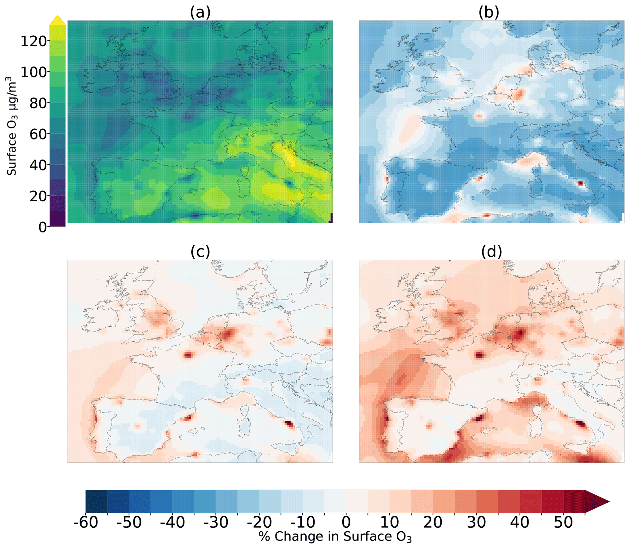
Figure A11 Mean O₃ in June, July and August for each scenario. Panel (a) shows this metric for the CMIP6 2014 simulation. Panels (b), (c) and (d) show the percentage change from this for SSP1-2.6, SSP2-4.5 and SSP3-7.0 respectively.

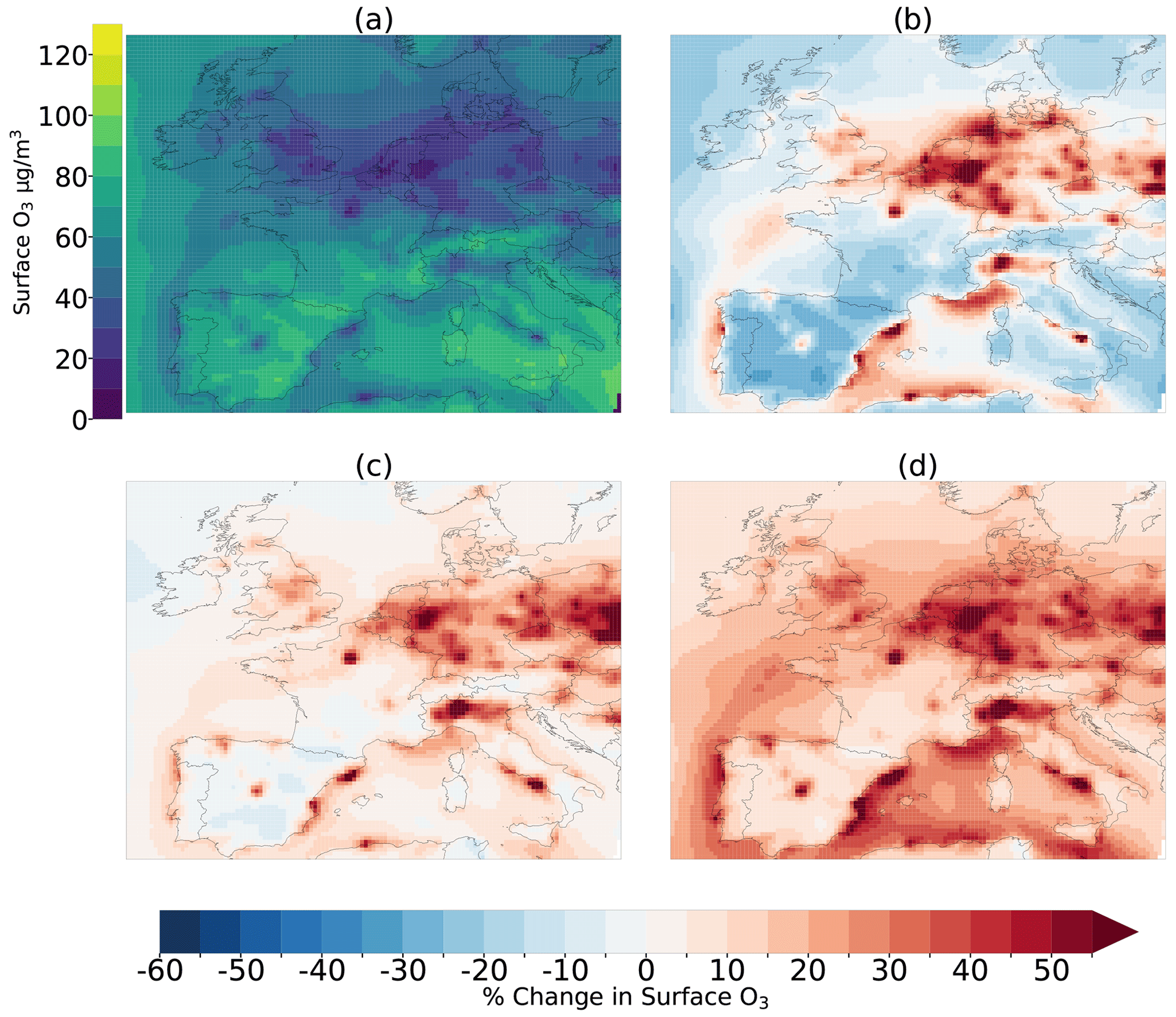
Figure A12 Mean O₃ in September, October and November for each scenario. Panel (a) shows this metric for the CMIP6 2014 simulation. Panels (b), (c) and (d) show the percentage change from this for SSP1-2.6, SSP2-4.5 and SSP3-7.0 respectively.