the Creative Commons Attribution 4.0 License.
the Creative Commons Attribution 4.0 License.
 | 23 Sep 2024
Aerosol composition, air quality, and boundary layer dynamics in the urban background of Stuttgart in winter
Wei Huang
Xiaoli Shen
Ramakrishna Ramisetty
Junwei Song
Olga Kiseleva
Christopher Claus Holst
Basit Khan
Thomas Leisner
Aerosol distributions are of great relevance for air quality, especially for cities like Stuttgart, which has limited air exchange due to its location in a basin. We collected a comprehensive set of data from remote sensing and in situ methods including radiosondes for the urban background of downtown Stuttgart to determine the impact of boundary layer mixing processes on local air quality and to evaluate the simulation results of the high-resolution large eddy simulation (LES) model PALM-4U at 10 m grid spacing. Stagnant meteorological conditions caused accumulation of aerosols, and chemical composition analysis shows that ammonium nitrate (37 ± 9 %) and organic aerosol (OA; 34 ± 9 %) dominated during this winter study. Case studies show that clouds during previous nights can weaken temperature inversion and accelerate boundary layer mixing after sunrise by up to 3 h. This is important for ground-level aerosol dilution during the morning rush hour. Furthermore, our observations validate results of the LES model PALM-4U in terms of boundary layer heights and aerosol mixing for 48 h. The simulated aerosol concentrations follow the trend of our observations but are still underestimated by a factor of 4.5 ± 2.1 due to missing secondary aerosol formation processes and uncertainties of emissions and boundary conditions in the model. This paper firstly evaluates the PALM-4U model performance in simulating aerosol spatio-temporal distributions, which can help to improve the LES model and to better understand sources and sinks for air pollution as well as the role of horizontal and vertical transport.
- Article
(4802 KB) - Full-text XML
-
Supplement
(2316 KB) - BibTeX
- EndNote


The global and regional distribution of aerosol particles is of great concern, partly because these particles are much more visible than gaseous pollution (Chan and Yao, 2008; Guo et al., 2009; Li et al., 2016) and because they have discernible adverse effects on human health (Pöschl, 2005; Shiraiwa et al., 2017). Moreover, airborne particles critically impact Earth's climate through aerosol direct and indirect effects (Kiehl and Briegleb, 1993; Ramanathan et al., 2001; Ackerman et al., 2004; Stocker, 2014; Guo et al., 2017). Regional air quality is greatly affected by the temporal and spatial distribution of aerosol within the planetary boundary layer (Stanier et al., 2004; Li et al., 2017), which is related to the emission, transformation and transport of aerosol particles. In particular, transport depends on local boundary layer structure and meteorological conditions.
The daytime planetary boundary layer (PBL) is typically about 1–2 km thick (10 %–20 % of the troposphere) from the ground surface but can diurnally vary from 10 m to 4 km or more (Stull, 1988). Almost all land-based life on Earth takes place in the PBL. On larger scales, the PBL greatly affects the whole atmospheric system and determines the exchange of heat, moisture, and momentum between the Earth's surface and the free troposphere (Garratt, 1994; Medeiros et al., 2005). The top of the PBL, typically referred to as the boundary layer height (BLH), marks the transition from the layer of thorough mixing due to turbulence to the free troposphere where mixing is comparatively small. The fundamental definition of the PBL has traditionally been turbulence based. If the mixing is induced by convection, it is also called the convective boundary layer (CBL), and during night-time it is referred to as the nocturnal boundary layer (NBL) or stable boundary layer (SBL). The boundary layer is a turbulent layer adjacent to the Earth's surface layer (Stull, 1988).
Many methods have been used to investigate the atmospheric parameters (e.g wind and temperature) and constituents (e.g. water and particles) within the PBL. In situ measurements, such as weather sensors deployed at ground-level meteorological stations or towers that can provide information at the ground level, were used to study the heat, moisture, and momentum in the boundary layer (Stull and Eloranta, 1984; Gentine et al., 2016). In addition, instruments for ground aerosol characterization like a condensation particle counter (CPC), scanning mobility particle sizer (SMPS), optical particle counter (OPC), and aerodynamic particle sizer (APS) are used to investigate the aerosol concentration and particle size information (Bates et al., 2000, 2002; Quan et al., 2013; Shin et al., 2014). Mass spectrometry can be used to study the chemical composition of aerosol and gas (Nash et al., 2006; Jordan et al., 2009; Aljawhary et al., 2013). Furthermore, these in situ instruments can also be deployed on aircraft, balloons, and unoccupied aerial vehicles (UAVs) to get vertical profiles of aerosol concentrations and components in and above the boundary layer (Lenschow, 1986; Greenberg et al., 1999; Neff et al., 2008; Reineman et al., 2016; Kim and Kwon, 2019; Y. Zhang et al., 2020).
In addition to these in situ measurements, remote sensing methods including minisodar (Prabha et al., 2002), sonic anemometer (Neff et al., 2008), and microwave radiometer (Westwater et al., 1999), as well as lidar (light detecting and ranging), are also used to investigate boundary layers. Lidar is an advanced active sensing instrument that can provide range-resolved and continuous measurements with high temporal (e.g. from seconds to several minutes) and spatial (e.g. from several metres to tens of metres) resolution. By now, several types of lidar instruments including temperature lidar (Hammann et al., 2015), Doppler wind lidar (Floors et al., 2013), aerosol lidar (Hennemuth and Lammert-Stockschlaeder, 2006), and water vapour lidar (Froidevaux et al., 2013) have been used to measure the boundary layer structures. The temperature lidar can provide the thermal structure of the boundary layer, whereas the Doppler wind lidar can offer wind and turbulence information. The aerosol and water vapour lidar can illustrate the distribution of these atmospheric components within the boundary layer. However, most lidars provide interpretable data at distances from tens of metres to around 1000 m, which makes it difficult to get valid measurements near the surface level for most vertically pointing lidar system. As the height especially of the nocturnal boundary layer varies only from tens of metres to 200 m (Stull, 1988), it is not easy to determine the structure of the NBL with vertically pointing lidar. But a scanning lidar has the capability to conduct off-zenith measurements or horizontal measurements, hence allowing vertical profiles of aerosols within the nocturnal boundary layer to be deduced.
Large eddy simulations (LESs) constitute a mathematical method for turbulence used in computational fluid dynamics and has been used to simulate atmospheric boundary layers with high spatial resolutions (Mason, 1989; Stoll et al., 2020; Spiga et al., 2021) in the past few years, mainly due to increasing amounts of computational resources being available for research in this field. Khan et al. (2021) developed an atmospheric chemistry model coupled to the turbulence-resolving PALM model system 6.0 (Maronga et al., 2020) (a LES model) to investigate the evolution of gas pollutants (NOx, O3, and CO) in the city of Berlin, Germany. Slater et al. (2020) investigated the aerosol–radiation–meteorology feedback loop using a coupled LES in Beijing, which directly attributes the effect of aerosol loading on boundary layer evolution and aerosol mixing process. Wang et al. (2023) investigated air quality in Hong Kong SAR, combining coupled mesoscale–microscale modelling (WRF-Chem–LES) and in situ sensors to evaluate model performance for different spatial scales. Kurppa et al. (2019) firstly evaluated the vertical variation of aerosol number concentration and size distribution in a simple street canyon without vegetation in Cambridge by embedding the sectional aerosol module SALSA2.0 (Kokkola et al., 2008, 2018) into the large eddy simulation model PALM (Maronga et al., 2020). Weger and Heinold (2023) assessed the impact of meteorology and urban topography on the microscale variability of urban air pollution using a LES and empirical orthogonal function (EOF) analysis for the Dresden basin. Their results showed that the model results are strongly sensitive to atmospheric conditions but generally confirm increased equivalent black carbon (eBC) levels in Dresden due to the topography. Although the LES has been widely used to study urban boundary layer dynamics, the comparison of LES results with observational data, especially with high-resolution lidar measurements, is rarely done, especially for detailed aerosol particle studies.
The city of Stuttgart is an important industrial centre in southwest Germany with a population of more than 600 000 in a metropolitan area of 2.6 million inhabitants. The city is located in the steep valley of the Neckar River, a basin-like area surrounded by a variety of hills, small mountains, and valleys. The undulating terrain would induce a low wind speed and weak synoptic atmospheric circulation, which typically hinders the dispersion of aerosol particles (Schwartz et al., 1991; Hebbert et al., 2012). As one of the most polluted cities in Germany, air quality has been a long-standing concern in Stuttgart (Schwartz et al., 1991; Süddeutsche Zeitung, 2016; LUBW, 2016; Huang et al., 2019). The state environmental protection agency, LUBW (Landesanstalt für Umwelt Baden-Württemberg), attributes 58 % of the annual mean PM10 at their monitoring station “Am Neckartor” in downtown Stuttgart to road traffic (45 % abrasion, 7 % exhaust, 6 % secondary formation), 8 % to small and medium-sized combustion sources, and 27 % to the regional background (Leiber et al., 2016). Mayer (1999) showed the temporal variability of urban air pollutants (NO, NO2, O3, and Ox (sum of NO2 and O3)) caused by motor traffic in Stuttgart based on more than 10 years of recorded data, with higher NO concentrations in winter and higher Ox concentrations in summer. Kiseleva et al. (2021) investigated nocturnal atmospheric conditions and their impact on air pollutant concentrations in the city of Stuttgart, focusing on the connection between atmospheric conditions and air pollutants using radiosonde, wind lidar, and microwave radiometer data and data from near-surface meteorological and air quality observations and turbulence evaluations for PALM-4U conducted later (Kiseleva et al., 2024). Ground-based remote sensing methods were used by Zeeman et al. (2022) to assess boundary layer and local flow processes. For the summer season, Samad et al. (2023) described extensive observational efforts to capture many aspects of atmospheric processes in Stuttgart. Samad and Vogt (2020) assessed the effect of traffic density and cold airflows on the urban air quality in Stuttgart with the complex topography. The results show that the local road traffic emissions account for 52 % for NO2 concentrations and 47 % for PM10 concentration, and the city was less polluted when cold airflows blew from west and southwest directions. Figure S1 in the Supplement shows the seasonal average of PM10 in four LUBW monitoring stations and the average values of these four stations in Stuttgart from 2012 to 2022. This figure shows that the concentration of PM10 is highest in winter (December, January, and February), and the Am Neckartor monitoring station in downtown Stuttgart shows the highest concentration compared with other monitoring stations. Hence, this detailed study on the aerosol evolution and its related boundary dynamics near Am Neckartor during winter can improve our understanding of the mechanisms driving air quality dynamics in Stuttgart.
For the research presented in this paper, we collected comprehensive datasets from one field campaign conducted between 5 February and 5 March 2018 in downtown Stuttgart and simulation data from a LES (PALM-4U) to study the boundary layer dynamics and air quality in the Stuttgart basin. One scanning aerosol lidar, one wind lidar, one microwave radiometer, and one mobile container equipped with aerosol characterization instrumentation and a meteorological sensor, as well as radiosondes, were used in this study. In addition, the large eddy simulation model system, PALM-4U, was used to simulate the airflow and aerosol evolution in the Stuttgart basin domain over a 48 h period. Huang et al. (2019) reported the organic aerosol chemical composition and volatility for both winter and summer, which provided insights into the seasonal variation of the molecular composition and volatility of ambient OA particles and into their potential sources. However, this work is more focused on the boundary layer evolution and associated aerosol spatial distribution within the boundary layer based on the comparison of the comprehensive dataset from remote sensing and in situ measurements and model simulation. To the best of our knowledge, the paper firstly used the above comprehensive datasets to demonstrate boundary layer dynamics and the aerosol mixing process. The objective of this work is to study the characteristic evolution of the wintertime boundary layer and to investigate the impact of vertical and horizontal mixing on surface aerosol concentrations by combining the aforementioned datasets. Our study, therefore, adds an important piece of information on air quality in Stuttgart by investigating the boundary layer dynamics, aerosol chemical composition, and aerosol physical properties.
This paper is organized as follows. Section 2 describes the remote sensing and in situ methods as well as the implementation of the PALM-4U model. Details of the evolution of the boundary layer and the impact of mixing processes on aerosol concentrations are discussed in Sect. 3. In the final section, we provide conclusions.
This study is based on a dataset collected in the structured terrain characterizing the city of Stuttgart in southwestern Germany (refer to Fig. 1). The area of interest includes the relatively broad Neckar valley (width about 2 km), which is orientated from southeast to northwest, and the basin-shaped valley called the Stuttgart basin (about 2.5 km×2.5 km), which opens up to the Neckar valley in the northeast. The valley floor is approximately at an altitude of 300 m above mean sea level (m a.s.l.) and surrounded by hills with ridge heights of up to 520 m a.s.l. A mobile measurement container was installed on a railway bridge in Rosenstein Park (RSP; 247 m a.s.l.; see Fig. 1b) in downtown Stuttgart. Our measurements were done in a park area in downtown Stuttgart with sufficient distance to heavy traffic or other substantial air pollution sources. There were no significant emissions from the electric train tracks nearby. Therefore, we can indeed classify this as an urban background site in a downtown area. Please note that the Am Neckartor monitoring station is about 1.5 km southwest of the measurement location used in this study. A scanning aerosol lidar was installed on the roof of this container equipped with in situ instruments including a high-resolution time-of-flight aerosol mass spectrometer (HR-TOF-AMS), an aethalometer (AE 51), a condensation particle counter (CPC), an optical particle counter (OPC; Fidas-200), trace gas sensors, and meteorological sensors. For further details on the instrumentation, see also Huang et al. (2019). In addition, radiosondes launched at Schnarrenberg (SB; 321 m a.s.l.; see Fig. 1b) by the German weather service (DWD) provided vertically resolved meteorological parameters. A wind lidar and a microwave radiometer deployed at the Stuttgart town hall (TH; 275 m a.s.l., 3.5 km southwest of the measurement container with the lidar; see Fig. 1b) measured vertically resolved wind and temperature, respectively. Furthermore, a LES applying PALM-4U (Maronga et al., 2020) was performed to simulate the complex airflow and resulting aerosol transport in this area.
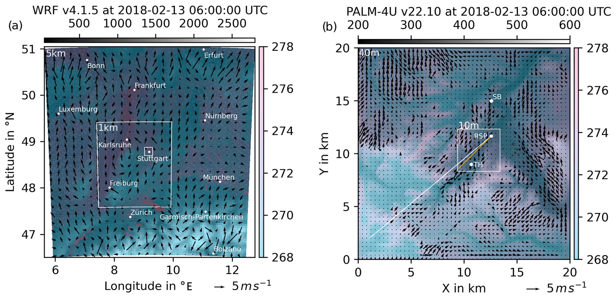
Figure 1The 2 m temperatures (colour) and 10 m winds (vectors) from the WRF simulation over the model topography height in metres above sea level (brightness) are shown in panel (a). The white labels serve for orientation and the white lines mark the approximate domain boundaries. The “5 km” and “1 km” labels shown in the upper-left corner of boundaries represent grid spacing. Around Stuttgart, the PALM-4U outer domain boundaries are shown by a small white box. In panel (b) the PALM-4U domains are presented using the same type of visualization for the same model output time. Shown are the potential temperature and horizontal winds on the second model level above the surface (i.e. 15 m a.g.l.). The labels indicate measurement site locations, and the white line indicates the aerosol laser scan beam, while the orange line indicates the location of the vertical section evaluated from PALM-4U (RSP: Rosenstein Park). The “40 m” and “10 m” labels shown in the upper-left corner of boundaries represent grid spacings.
2.1 Remote sensing
2.1.1 Scanning aerosol lidar
The scanning aerosol lidar (Raymetrics Inc., type LR111-ESS-D200, named KASCAL) used in this campaign is a mobile scanning system with an emission wavelength of 355 nm. The laser pulse energy and repetition frequency are 32.1 mJ and 20 Hz, respectively. The laser head, 200 mm telescope, and lidar signal detection units are mounted on a rotating platform allowing zenith angles from −7 to 90° and azimuth angles from 0 to 360°. This lidar works automatically, scheduled, and continuously via software developed by Raymetrics. Detailed information can be found at https://www.raymetrics.com/product/3d-scanning-lidar, last access: 1 September 2022 (Avdikos, 2015; Zhang et al., 2022). The lidar was put on the roof of the container and conducted zenith scanning measurement with elevation angles from 90 to 5° with a step of 5°. The beam of the lidar was directed along the basin axes as shown by a white line in Fig. 1.
For the data analysis and calibration of the system, we followed the quality standards of the European Aerosol Research Lidar Network (EARLINET) (Freudenthaler, 2016). The data analysis for the zenith measurements employed the Klett–Fernald method to obtain vertical profiles of backscatter coefficients. These vertical aerosol backscatter coefficients were used as the reference values for other elevation angle measurements.
The atmospheric boundary layer heights were determined from lidar data using the Haar wavelet transform (HWT) method (Pal et al., 2010). The method is defined as
where wf is the covariance transform value; X(z) is the range-corrected lidar signal defined as ; and is the Harr wavelet function, defined as follows:
The dilation a is set to be 75 m in this paper, and b is the translation parameter. zmin and zmax are the lower and upper heights of the lidar signal profile, respectively.
2.1.2 Doppler wind lidar
The Doppler wind lidar principle relies on the measurement of the Doppler frequency shift of laser radiation backscattered by the particles in the air (dust, aerosols). WindCube v2 (Leosphere, Vaisala) measures wind speed with a Doppler beam swinging (DBS) technique (Rao et al., 2008), where an optical switch is used to point the lidar beam in the four cardinal directions (north, east, south, and west) at an elevation angle of 62° from the ground, and it allows us to obtain vertical wind profiles of wind speed and direction, turbulence, and wind shear up to a height of 200 m. Detailed information about WindCube v2 is given on the Vaisala home page (Vaisala, 2021).
2.1.3 Microwave radiometer
The microwave profiler HATPRO was manufactured by Radiometer Physics GmbH, Germany (RPG) as a network-suitable microwave radiometer with very accurate retrievals of liquid water path (LWP) and integrated water vapour (IWV) at high temporal resolution (1 s). The spectral characteristics of the instrument also make it possible to observe the temperature profile and also, to a limited extent, the humidity profile (Löhnert and Maier, 2012).
2.2 In situ measurements
The WS700 meteorological sensors (Lufft GmbH) provided air temperature, relative humidity, wind direction, wind speed, global radiation, pressure, and precipitation data. Different trace gas sensors measured O3, CO2, NO2, and SO2 gas compositions. An aethalometer (AE51; Aethlabs Inc.) measured the temporal variability of equivalent black carbon (eBC) concentrations (Petzold et al., 2013). An HR-ToF-AMS equipped with an aerodynamic lens (Williams et al., 2014) was installed in a mobile container to continuously measure total non-refractory particle mass as a function of size (up to 2.5 µm particle aerodynamic diameter) at a temporal resolution of 30 s. The AMS inlet was connected to a PM2.5 head (flow rate 1 m3 h−1; Comde-Derenda GmbH) and a stainless-steel tube of 3.45 m length. The AMS data were analysed with AMS data analysis software packages SQUIRREL (version 1.60C) and PIKA (version 1.20C). Positive matrix factorization (PMF; Paatero and Tapper, 1994; Paatero, 1997) was applied for AMS data to identify different aerosol source factors for source appointment (Ulbrich et al., 2009; DeCarlo et al., 2010; Zhang et al., 2011; Mohr et al., 2012; Canonaco et al., 2013; Crippa et al., 2014; Shen et al., 2019). This allows us to differentiate organic aerosol in terms of, for example, hydrocarbon-like OA (HOA), cooking-related OA (COA), nitrogen-enriched OA (NOA), biomass burning OA (BBOA), semi-volatile oxygenated OA (SV-OOA), and low-volatility oxygenated OA (LV-OOA). The mass spectra of these five OA factors resolved from the PMF analysis are shown in Fig. S2. These in situ data were averaged over 10 min. Detailed information about in situ measurements and aerosol chemical composition is introduced in Huang et al. (2019).
In addition to in situ container measurements, radiosondes at Schnarrenberg meteorological station (SB; see Fig. 1b) were launched by the German weather service (DWD) to measure the vertical profile of meteorological parameters (e.g. temperature, humidity, pressure, and wind). The vertical profiles of temperature and humidity were used to determine boundary layer heights. Detailed descriptions of boundary layer retrieval methods were introduced in previous publications (Hennemuth and Lammert-Stockschlaeder, 2006; Liu and Liang, 2010; Seidel et al., 2010; Guo et al., 2016).
2.3 Modelling
2.3.1 WRF setup
The Weather Research and Forecasting (WRF) model version 4.1.3 (Skamarock et al., 2021) was forced by ERA5 reanalysis data (Hersbach et al., 2020) and local climate zone (LCZ) data (Demuzere et al., 2022a, b) to produce consistent meteorological fields from 11 to 14 February 2018 as forcing for the microscale simulation. Two nested domains with 5 and 1 km horizontal grid spacing have been placed such that Stuttgart is located at the centre and a sufficiently large part of the European continent is covered, to allow for all relevant flow fields to evolve appropriately.
ERA5 is the fifth-generation European Centre for Medium-Range Weather Forecasts (ECMWF) atmospheric reanalyses of the global climate (Hersbach et al., 2020). ERA5 provides multiple climate variables at a spatial resolution of 0.25° (approximately 30 km) for the globe every hour, with 137 levels from the surface up to 0.01 hPa (around 80 km height) (https://doi.org/10.24381/cds.adbb2d47).
2.3.2 PALM-4U setup
PALM-4U (Maronga et al., 2020) is a model system that has been developed to simulate a wide range of urban microscale processes. The centre of this model system is the large eddy simulation model PALM (Raasch and Schröter, 2001) based on non-hydrostatic, filtered, incompressible Navier–Stokes equations in Boussinesq-approximated form. To force this microscale model for realistic cases, meteorological data is required for initial and boundary conditions, as well as detailed information about the modelled surface properties (e.g. topography). Details of the model pipeline are described below.
For the successful simulation of the complex, topographically forced flows around Stuttgart, a relatively large model domain is required. Two nested domains spanning 20 km × 20 km and 4 km × 4 km, with 40 m and 10 m grid spacing, respectively, have been set up. The geostatic data required for these two domains were described by Heldens et al. (2020). The output of the WRF simulation was processed with the PALM-4U package tools for the 48 h period from 12 to 14 February 2018 to create initial and boundary conditions to force PALM-4U. Wind, temperature, moisture, radiative fluxes, and soil variables were assimilated from these WRF data.
Particulate matter (PM10) was simulated with the phstatp chemical mechanism, which allows for emissions, transport, and dry deposition (Kurppa et al., 2019) but neglects other aerosol processes. The emissions sources of the PALM-4U model were parameterized by street type (Maronga et al., 2020), and initial boundary condition profiles were approximated from observed profile values at the simulation initialization time. These profiles persisted as constant boundary conditions for the entire 48 h period. Note that the nested domain is located at a distance of approximately 8 km from the outer boundary, at which this constant nocturnal profile is forced. During stable nocturnal conditions, the profile properties are mostly conserved throughout the transport process (assuming small vertical transport). Convective daily conditions produce adequately mixed particulate profiles at the child domain's boundary, due to the sufficient distance (larger than 3 times the boundary layer height). This simplified approach leads to particulate concentration fields that approach a balance between dry deposition and emission.
The model output was averaged in time over 10 min intervals and output above the model surface (i.e. terrain-following) up to heights of 1500 m a.g.l. to maximize compatibility with the measured data.
In this section, we will firstly review the measurements during this field campaign. Then we will discuss our result on the correlation of boundary layer heights with ground-level aerosol concentrations, especially the relationship at night-time. Afterwards, two selected cases were used to demonstrate the boundary layer evolution and aerosol mixing processes within the boundary layer. Finally, the LES (PALM-4U) was used to simulate the boundary layer processes and to investigate the aerosol transport and mixing processes within the boundary layer in the context of the local and regional flow properties.
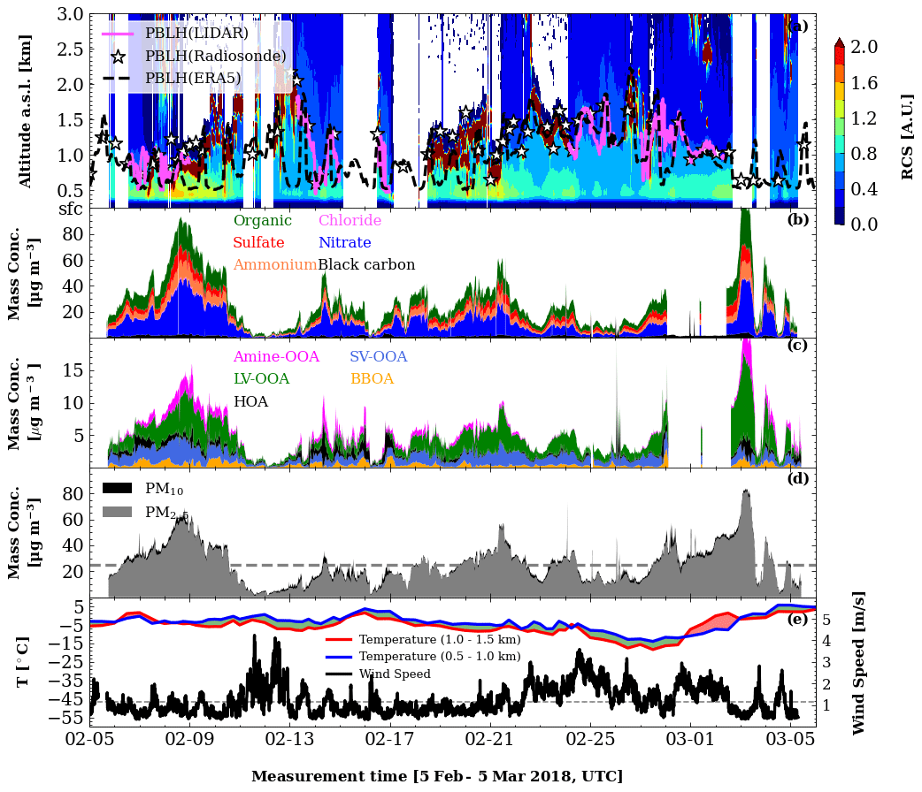
Figure 2Time series of the range-corrected lidar signal (contour) and boundary layer heights derived from the scanning aerosol lidar (pink line), radiosonde (stars), and ERA5 dataset (dashed black line) (a); the aerosol mass concentrations for different chemical components (b); five-factor PMF solutions of organic aerosol (c); the particulate matter concentrations measured by OPC (d); and the temperatures at two different altitude levels measured by radiosondes as well as wind speed measured at 10 m a.g.l. (e).
Figure 2a shows time series of the range-corrected lidar signal (RCS) for the whole observation period as well as boundary layer heights retrieved from lidar during periods that are cloud-free up to 3 km a.g.l. In addition, boundary layer heights derived from radiosonde and ERA5 data are also shown in this figure, as indicated by stars and a dashed black line, respectively. This panel shows good agreement in boundary layer heights among lidar and radiosonde measurements as well as the ERA5 dataset. The correlation of boundary layer height between lidar and radiosonde measurements is shown in the left panel of Fig. S3, which shows that the boundary layer heights retrieved from lidar and radiosonde agree well with each other, with a slope of 1.10 ± 0.14 and a Pearson correlation coefficient of 0.86. The correlation of boundary layer heights between lidar and ERA5 reanalysis is shown in the right panel of Fig. S3, which shows a slope of 0.70 ± 0.07 and a Pearson correlation coefficient of 0.61. The boundary layer heights from the ERA5 reanalysis are systematically lower than those from lidar and radiosonde retrieval but still show the same trend as the lidar measurements. This underestimation was also reported by Dias-Júnior et al. (2022). The inconsistency between observations and ERA5 data is mainly due to the different spatial resolutions of the methods and the relatively complex topography in Stuttgart. The evolution of aerosol composition measured by HR-TOF-AMS as well as the eBC concentrations are shown in Fig. 2b. The data indicate that nitrates (37 ± 9 %) dominated in aerosol chemical composition due to high NOx emissions and lower air temperatures in winter, inhibiting the evaporation of ammonium nitrate (Xie et al., 2020; Z. Zhang et al., 2020). The positive matrix factorization (PMF) analysis of organic aerosol (OA) factors shown in Fig. 2c illustrates that low-volatility oxygenated organic aerosol (LV-OOA) components are dominant (42 ± 15 %) during these measurements. These compounds are mostly attributed to aerosol from regional transport (Song et al., 2022). A detailed analysis of the chemical composition of the aerosol in Stuttgart can be found in Huang et al. (2019). The average temperatures in two altitude ranges (0.5–1.0 and 1.0–1.5 km) measured by radiosondes and wind speed at 10 m above ground level measured by the meteorological sensor (WS700) is shown in Fig. 2e. The temperature inversion (red area between two temperature lines) and low wind speed periods coincide with an accumulation of aerosols (e.g. from 6 to 8 February and from 28 February to 2 March). The obvious temperature inversion and low wind speeds during the above two periods are labelled as stagnant meteorological conditions, which suppressed convection in the troposphere, hence causing a shallow and nocturnal boundary layer and accumulation of aerosols at ground level. Stagnant conditions are also an important reason for air pollution in mega cities (Huang et al., 2018; Katsoulis, 1988; Ji et al., 2014).
Figure S4 shows the vertical profile of temperature (left) and wind speed (right) during the polluted period and a less polluted period. The polluted period is defined for concentration of PM10 exceeding the ambient air quality standard for the European Union (25 µg m−3; https://www.transportpolicy.net/standard/eu-air-quality-standards/, last access: 3 July 2023), which is indicated by the dashed grey line in Fig. 2d. These average profiles of temperature and wind speed shown in Fig. S4 were calculated after excluding the data collected on weekends to avoid the influence of local emission differences between weekdays and weekends. Figure S4 shows a strong temperature inversion and low wind speed during the polluted period, which is the typical structure of vertical thermal and dynamics during stagnant conditions (Huang et al., 2018).
3.1 Correlation between boundary layer heights and ground-level aerosol concentrations
Figure S5a, e, and i show the correlation between boundary layer heights and PM10, eBC, and BBOA concentrations for three different subsets of data, respectively. The colour of the scatter points indicates the relative humidity. For all PM10 data points, an anti-correlation, as shown in Fig. S5a, was found for boundary layer heights above 900 m (, Pearson correlation coefficient, same hereafter). This anti-correlation means that a deeper boundary layer diluted the aerosol, while a shallower boundary layer concentrated aerosol at the ground level. The aerosols were diluted by transporting them from a near-ground level to higher altitudes during boundary layer mixing process. However, we also found a positive correlation between PM10 and boundary layer heights for boundary layer heights below 900 m a.s.l. (R=0.32). This positive correlation is also reported in Yuval et al. (2020) and typically coincided with low wind speed and high relative humidity, indicating typical properties of the nocturnal boundary layers.
Then, the data were divided into three groups for three different time periods – morning (04:00–10:00 UTC) (b, f, j), afternoon (12:00–18:00 UTC) (c, g, k), and night (18:00–04:00 UTC) (d, h, l). The correlation between the boundary layer and surface aerosol concentrations (PM10) in the these three subplots (b–d) is positive for PBL heights below 900 m a.s.l. (R=0.31 (Fig. S5b), 0.58 (Fig. S5d)) and weaker but negative for larger PBL heights ( (Fig. S5b), −0.49 (Fig. S5c), −0.22 (Fig. S5d)). The correlation between boundary layer heights and eBC, as well as BBOA concentrations shown in Fig. S5, revealed that the eBC and BBOA concentrations are always anti-correlated with the boundary layer heights ( (Fig. S5e), 0.21 (Fig. S5i)). The reason for the positive correlation between PM10 and boundary layer height below 900 m a.s.l. is the fact that the local emissions and aerosol water are taken up during the night and in the early morning. The reason for only anti-correlation between the boundary layer heights and eBC, as well as BBOA concentrations, is that the eBC and BBOA emitted particles from sources like biomass burning or traffic are smaller and less hygroscopic and thus could be diluted by boundary layer evolution.
A good case to illustrate this phenomenon is shown in Fig. 4. The chemical composition measured by the AMS is shown in Fig. 4b. From this figure, we found that the mass concentration of various aerosol components (e.g. ammonium sulfate, ammonium nitrate) increased from 13 February at 18:00 to 14 February at 05:00 UTC, while the boundary layer heights increased slowly during this time period, which caused a positive correlation between the boundary layer and PM10 concentration. However, the eBC and BBOA concentrations shown in Fig. 4c and d are constant in the night-time. Hence, the PM10 concentrations can be correlated with boundary layer heights, while eBC and BBOA concentrations are always anti-correlated with boundary layer heights.
The above statistical data analysis of the correlation between ground-level aerosol concentrations and the boundary layer heights is based on data collected during 1 month. More data were analysed to support this relationship. Figure S6 shows the diurnal variations of PM10 and the boundary layer heights based on 2-year data from 1 January 2020 to 31 December 2021 in Stuttgart. The PM10 concentrations are the hourly reported data by LUBW, and the boundary layer heights are from the ERA5 dataset. Figure S6 shows a positive correlation between boundary layer heights and PM10 concentrations between 04:00 and 08:00 UTC as shaded in Fig. S6, and this positive correlation is possibly related to local morning emission or water take up during the morning rush hour. In addition, the increasing boundary layer after sunrise (08:00–12:00 UTC) diluted the aerosol within the boundary layer, thus causing a decrease in PM10 concentrations.
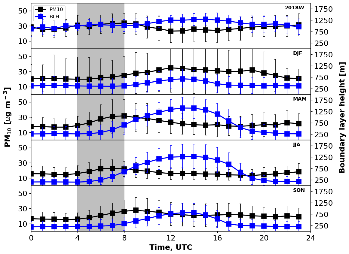
Figure 3Diurnal variations of PM10 concentrations (black) and the boundary layer heights (blue) for the winter of 2018 based on our measurements (top panel) as well as for different seasons (winter: DJF, spring: MAM, summer: JJA, spring: SON) based on 2-year data from 1 January 2020 to 1 January 2022 in Stuttgart. The 2-year PM10 concentrations are hourly reported data by LUBW, and the boundary layer heights are from ERA5 data. The grey-shaded time interval shows correlations between BLH and PM10 for all seasons.
The diurnal variations of PM10 concentrations and the boundary layer heights are shown in Fig. 3 for the winter of 2018 based on our measurement (top panel) as well as different seasons based on LUBW and ERA5 data. This also shows that the ground-level PM10 concentrations are correlated with boundary layer heights from 04:00 to 08:00 UTC for all datasets. However, the strength of the correlation is different for different seasons. The spring (MAM) shows the strongest correlation (Pearson correlation coefficient: 0.83), while the winter (DJF) shows the weakest correlation (Pearson correlation coefficient: 0.26). In addition, the summer has the highest mixing layer height (1283 ± 399 m) while the winter has the lowest mixing layer height (682 ± 542 m) as expected due to the solar radiation being strongest in summer while weakest during winter. The ground-level PM10 aerosol concentrations are anti-correlated with mixing layer heights and show the highest concentrations during winter (33 ± 32 µg m−3) and the lowest concentrations during summer (16 ± 7 µg m−3). From the correlation between PM10 concentrations and boundary layer heights, we conclude that the ground-level PM10 concentrations are anti-correlated with mixing layer heights but correlated with nocturnal boundary layer heights.
3.2 Boundary layer dynamics and surface level aerosol – case studies
In Fig. 2, the evolution of the boundary layer heights and their effect on surface aerosol mixing processes is illustrated for the whole measurement period. In this section, two cases (13–14 and 24–25 February 2018) are selected to demonstrate these processes in detail. The case from 13 to 14 February was selected due to the low wind speed (0.76 ± 0.35 m s−1). The low wind speed minimizes the impact of horizontal transport, allowing for more accurate analysis of local atmospheric conditions. Additionally, the clear skies during this 2 d period ensured sufficient solar radiation to fully engage the boundary layer dynamics. In contrast, the case from 24 to 25 February was chosen due to the presence of clear skies but with relatively stronger wind speeds (2.2 ± 0.6 m s−1). This selection allows for a comparative analysis of these two cases, highlighting the differences that wind speed can introduce to atmospheric conditions under otherwise similar solar radiation conditions.
Figure 4a shows the time series of lidar-retrieved vertical backscatter coefficients, the boundary layer heights (solid white line), the residual layer (RL) heights (dashed white line), and the boundary layer heights from the ERA5 dataset (dashed grey line), as well as the boundary layer heights retrieved from radiosondes (yellow triangles). Please note that the altitude used here is the height above sea level. The reason for using altitude instead of height above ground level is that the altitudes of these three observation stations are different, as shown in Fig. 1a. The vertically distributed backscatter coefficients are shown from the ground level to the free troposphere by merging zenith and near-horizontal (5° above the horizon) measurements. The time series of aerosol chemical composition measured by AMS is shown in Fig. 4b, and the PMF analysis result of the organic aerosol with five factors is shown in Fig. 4c. In addition, the potential temperatures (θ) from the microwave radiometer and turbulent kinetic energy (TKE) from wind lidar data are shown in Fig. 4e and f, respectively. Finally, the eBC concentrations and solar radiation are shown in Fig. 4d and g, respectively.
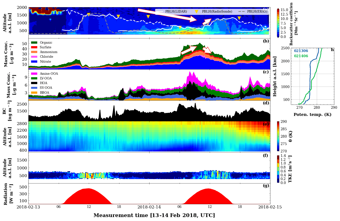
Figure 4Time series of backscatter coefficients from lidar measurements (contour plot), the boundary layer heights from lidar measurement (solid white line), the ERA5 dataset (dashed grey line), and DWD radiosonde (yellow triangle) as well as residual layer heights retrieved from lidar (dashed white line) (a); the aerosol mass concentrations measured by aerosol mass spectrometer (AMS) (b); five-factor positive matrix factorization (PMF) solutions of organic aerosol (c); black carbon concentrations (d); potential temperature measured by microwave radiometer (MWR) (e); turbulence kinetic energy (TKE) retrieved from Doppler lidar (f); and the global radiation measured by meteorological sensors (WS700) (g) for case 1 from 13 to 14 February 2018. The white arrows in panels (a) and (b) show the decreasing or increasing trends of boundary layer height. The plot on the right side shows the potential temperatures measured by radiosondes at 06:00 UTC on 13 and 14 February 2018.
The vertically extended backscatter coefficients in this figure show that most of the aerosol only stayed within the boundary layer or residual layer and could not reach the free troposphere, as stated in previous publications (Guo et al., 2009; Quan et al., 2013; Li et al., 2017; Su et al., 2018; Yuval et al., 2020). We also found that the mixing layer heights measured by lidar and radiosondes show good agreement in this case.
A decreasing trend of the residual layer height and a weakly increasing PBL height at around 550 ± 93 m a.s.l. can be seen during night-time. The shallow and nocturnal boundary layer and increased emissions during the morning rush hour (05:00–10:00 UTC) caused a rapid accumulation of aerosol near the surface, as can be seen from the low-altitude backscatter coefficients and ground-level in situ measurements. Driven by increased solar radiation after 10:00 UTC on 14 February, the boundary layer height increased and diluted the aerosol within the boundary layer, thus causing a decrease in aerosol concentrations at ground level. Furthermore, we found that the aerosol concentrations increased more during the morning rush hour (05:00–10:00 UTC) than during the evening rush hour (17:00–20:00 UTC), mainly due to the shallow boundary layer in the morning. The increased aerosol during the morning and evening rush hour is related to the emissions of traffic (HOA) and industry (amine-based OOA) as can be seen from the PMF analysis results shown in panel (c). At night-time, the potential temperature inversion shown in panel (e) and a small value of turbulent kinetic energy (TKE) shown in panel (f) indicate a stable and shallow boundary layer.
In order to investigate the effect of local emission on ground-level aerosol concentration, we need to normalize aerosol concentration by the boundary layer. The normalization was conducted in two following steps: (1) The boundary layer height was normalized to get unitless boundary layer height. (2) The aerosol concentration was multiplied by the unitless boundary layer height. Figure S7 shows a similar plot to Fig. 4 but with the ground-level aerosol concentration normalized by the boundary layer heights (daytime) or residual layer height (night-time) (Huang et al., 2023; Tsai et al., 2011). This figure shows that the nitrate aerosol particle mass increased from 3.9 to 10.8 µg m−3 in the morning rush hour (06:00–12:00 UTC) on 14 February 2018. While during the night-time (18:00–04:00 UTC), the nitrate aerosol particle mass increased from 2.5 to 3.9 µg m−3, the eBC concentrations decreased by more than 50 % from 1048 to 464 ng m−3. However, we need to be careful with this result, especially during night-time, as the aerosols are not well mixed but instead accumulate near the ground level. Hence, this normalization would be underestimated when considering the total aerosol concentration within the boundary layer. The aerosol horizontal transport source was not considered because the wind speed was 0.76 ± 0.35 (less than 1 m s−1 in most of time) from 18:00 13 February 2018 to 12:00 UTC 14 February 2018. The only considered source during this period is local emission. The reason for the increase in non-refractory particles concentrations but the decrease in eBC concentration is that the non-refractory particles were emitted during the night-time or take up water due to high relative humidity, while the emissions of eBC particles were diluted due to a slight increase in the nocturnal boundary layer during the night-time (Su et al., 2020).
Interestingly, we found in this case that the boundary layer height increased more slowly on the second day (14 February) than that on the first day (13 February). There was a time delay in the boundary layer convection during the second day despite the solar radiation being the same in this 2 d period (Fig. 4g). The reason for these different boundary layer evolutions is different vertical thermal structures, as can be seen in the vertical temperature profiles given in Fig. 4e and h. On the first day, the temperature inversion is weaker, and the TKE is larger than on the second day, as can be seen from Fig. 4e and f, which means that it takes a shorter time to transform the nocturnal boundary layer into the convective boundary layer. Hence, the boundary layer grew faster on the first day than on the second day. One explanation of these thermal structure differences for this 2 d period is the presence of clouds during the first night. They prevented longwave emissions and weakened the temperature inversion, which caused a neutral boundary layer during night-time. Furthermore, the boundary layer grew faster after sunrise due to this neutral boundary layer in the morning. Finally, the delay of the boundary layer convection process on the second day prevented diffusion of aerosol during the morning rush hour (05:00–10:00 UTC, 14 February), thus causing accumulation of aerosol at ground level, as shown in Fig. 4a–c. The conceptual schematic for this phenomenon is summarized in Fig. 5. The different boundary layer mixing in this 2 d period has a substantial impact on ground-level aerosol concentrations. As can be seen from Fig. 4, significantly more aerosol accumulated on 14 February due to lower boundary layer heights before 12:00 UTC. Here we assume similar emissions on these 2 weekdays.
.
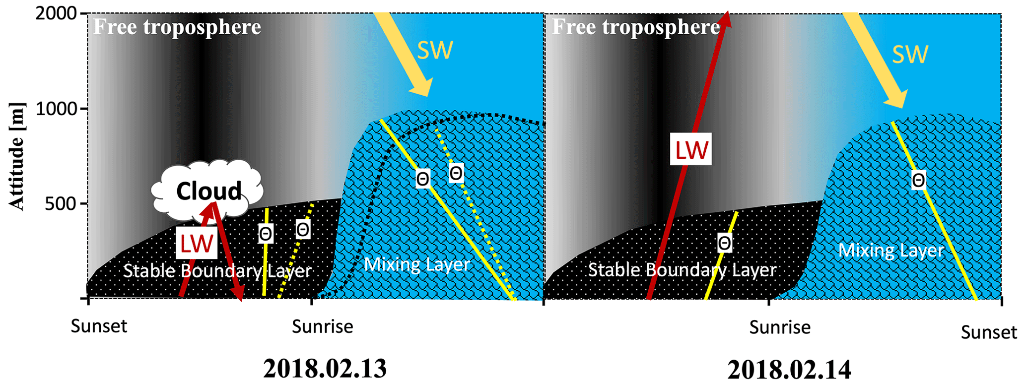
Figure 5Concept of boundary layer and the role of clouds in boundary layer evolution. The gold arrows indicate shortwave radiation, the red arrows indicate longwave radiation, the solid yellow lines indicate the potential temperature, the dotted yellow lines on the left side indicate the potential temperature on 14 February for comparison, the black textured areas indicated the stable boundary layer, the blue textured areas indicate mixing layer, and the dotted black line on the left side indicates the boundary layer height on 14 February for comparison. LW: longwave radiation. SW: shortwave radiation. θ: potential temperature.
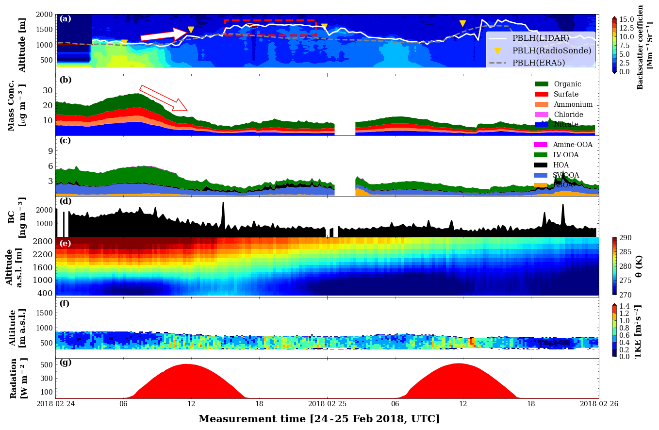
Figure 6Time series of backscatter coefficients from lidar measurements (contour plot), the boundary layer heights from lidar measurement (solid white line), the ERA5 dataset (dashed grey line), and DWD radiosonde (yellow triangle) (a); the aerosol mass concentrations measured by aerosol mass spectrometer (AMS) (b); five-factor positive matrix factorization (PMF) solutions of organic aerosol (c); black carbon concentrations (d); potential temperatures measured by microwave radiometer (MWR) (e); turbulence kinetic energy (TKE) retrieved from Doppler lidar (f); and the global radiation measured by meteorological sensors (WS700) (g) for case 2 from 24 to 25 February 2018.
Figure 6 shows the results during case 2, in which the same methods as in case 1 were applied, but different patterns were shown. The most obvious phenomenon is that a sharp decrease in aerosol concentrations from 07:00 to 12:00 UTC on 24 February was observed, even though the boundary layer heights only increased from 1042 to 1280 m a.s.l. In addition, the boundary layer heights did not decrease after sunset of 24 February, as shown in the red rectangle. Furthermore, the boundary layer heights measured by radiosondes are higher than those derived from lidar measurements, in contrast to case 1 (Fig. 4). The possible reason for the differences in boundary layer height for case 2 could be as follows: the radiosonde site (SB; 321 m a.s.l) is at a relatively higher altitude compared to the lidar site (RSP; 247 m a.s.l.), as shown in Fig. 1b. Additionally, the wind speed is much higher (2.2 ± 0.6 m s−1) for case 2, as shown in Fig. S8. This higher wind speed can induce updrafts, causing an increase in the boundary layer height. We also found that the aerosol concentrations at ground level were much lower on 25 February than those on 24 February, corresponding to a higher boundary layer on 25 February. Finally, the PMF analysis result shown in panel (c) shows a large fraction of LV-OOA for organic composition, which is typically more related to regional transport (Song et al., 2022).
Figures 4 and 6 showed different boundary layer evolution and different patterns of aerosol concentrations at ground level, even with a similar evolution of solar radiation, as shown in panel (g) of both figures. However, the evolution of temperature and wind is different, as shown in Fig. S8. Comparing the meteorological background in these two cases, we found that the temperature decreased more rapidly for case 2, as shown in the bottom panel of this figure. This decrease caused a lower temperature on 25 February. The temperature was below 0 °C, even during the day on 25 February. In addition, a higher wind speed was observed from 07:00 on 24 February to 16:00 UTC on 25 February for case 2. Then, the wind speed began to decrease, and the wind direction also changed from east to north from 16:00 UTC on 25 February. All this meteorological information indicates that a cold front passed by the observation station from 24 and 25 February, affecting local temperature and wind, thus having an impact on the boundary layer evolution and aerosol distributions in the boundary layer. The high wind speed during this cold front causes strong turbulence in the boundary layer, thus increasing the boundary layer heights, especially at night-time. In addition, this high wind speed also blew the local aerosol away and caused a low aerosol concentration on 25 February.
From the above two cases, we conclude that the evolution of the boundary layer was affected by related meteorological factors such as solar radiation, clouds, wind speed, and wind direction, which in turn affect the aerosol distribution in the boundary layer.
3.3 Comparison of large eddy simulations with observations
Case 1 outlined above is a good example of boundary layer evolution and aerosol mixing processes for 2 consecutive days. The comprehensive dataset collected during this case provided us a good opportunity to evaluate the LES model PALM-4U. To simplify, we use the altitude above the ground level (a.g.l.) to compare observational results with model simulations as the coordinate used in the model is the height above ground level.
The diurnal development of the boundary layer temperature fields as simulated by PALM-4U is shown in Fig. 7 as the time–height section above the RSP site, as indicated in Fig. 1b. Nocturnal cooling near the surface underneath the residual heat from the daytime and the stabilization of the boundary layer were captured by the model dynamics. During daytime, neutral, convective conditions were simulated with reoccurring stabilization, after longwave radiative cooling outweighed shortwave radiative heating at the surface. We found these thermally driven circulation processes to be simulated in a plausible way qualitatively, based on the observational data we compared the simulation results to. An exact quantitative comparison and an attribution of deviations have not been part of this study, as the focus was on the measured data. More detailed comparisons between two more scanning Doppler wind lidars and PALM-4U were conducted but will be published elsewhere, as this analysis of the model dynamics is not within the scope of this paper. Turbulence was evaluated for summer cases by Kiseleva et al. (2024).
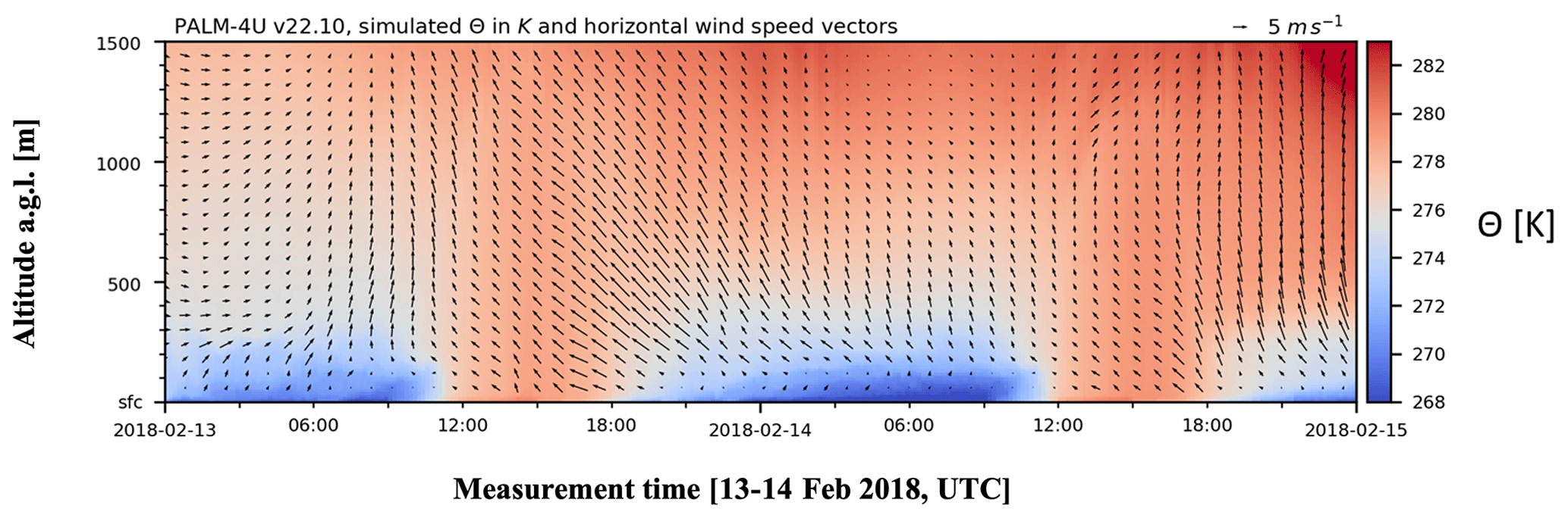
Figure 7Time–height cross section of simulated potential temperature (in K) and horizontal wind (in m s−1) at the RSP site from 13 February to 14 February 2018 from the surface to 1500 m a.g.l.
To compare aerosol spatial concentration between the PALM-4U simulation and observations, we convert lidar-derived extinction coefficients to PM2.5 concentrations using a conversion factor calculated from ground-level PM2.5 concentrations (OPC, Fidas200) and ground-level lidar-derived extinction coefficients. Figure S9 shows a good linear correlation between extinction coefficients and PM2.5 concentrations, with a slope of 78 182.0 ± 1132.0 and Pearson correlation coefficient of 0.822; this good correlation ensures the quality of this conversion. Figure 8 shows the time series of the PM2.5 concentrations retrieved from lidar measurements and PALM-4U. Figure 8c shows time series of PM2.5 concentrations from ground-level OPC measurements and from a PALM-4U simulation, which indicates that the simulated PM2.5 concentrations show a similar trend to the observational data except for the spin-up period (before 12:00 UTC 13 February) but underestimate the PM2.5 concentrations by a factor of 4.5 ± 2.1. The spin-up period ensures that the atmosphere is in balance with the new surface temperature and soil properties and that the atmospheric chemistry approaches an equilibrium state. The comparison of vertical extended PM2.5 concentrations from lidar measurement and the model simulation shows that PALM-4U agrees well with lidar observation in terms of boundary layer evolution and aerosol transport and mixing processes. This is in line with our objectives and the scope this study.
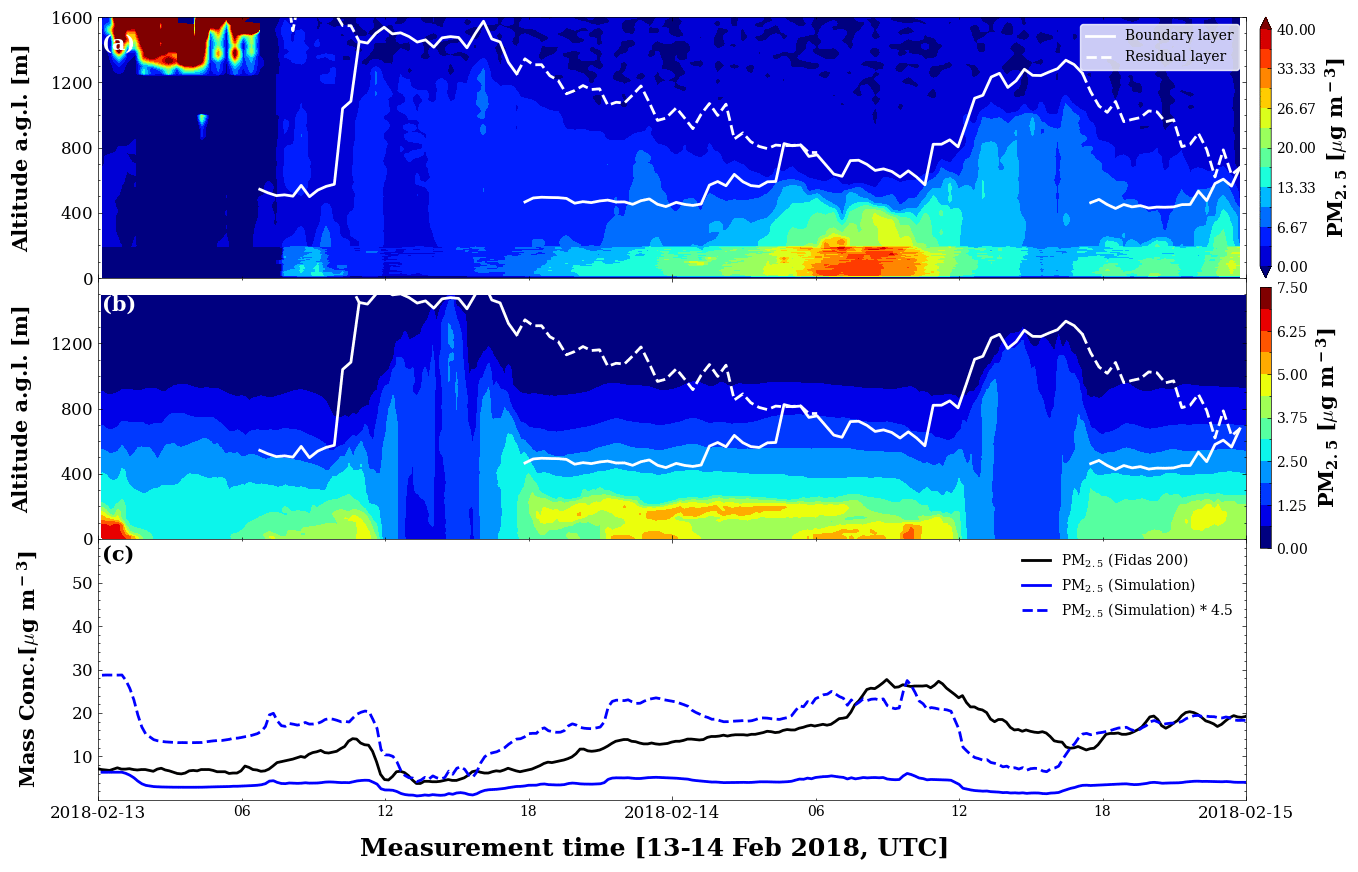
Figure 8Time series of the PM2.5 concentrations retrieved from lidar measurements (a) and PALM-4U (b), the boundary layer height (white line) and residual layer height (dashed white line) retrieved from lidar, and ground-level PM2.5 concentration measured by Fidas200 and modelled by PALM-4U (c) for case 1 from 13 to 14 February 2018.
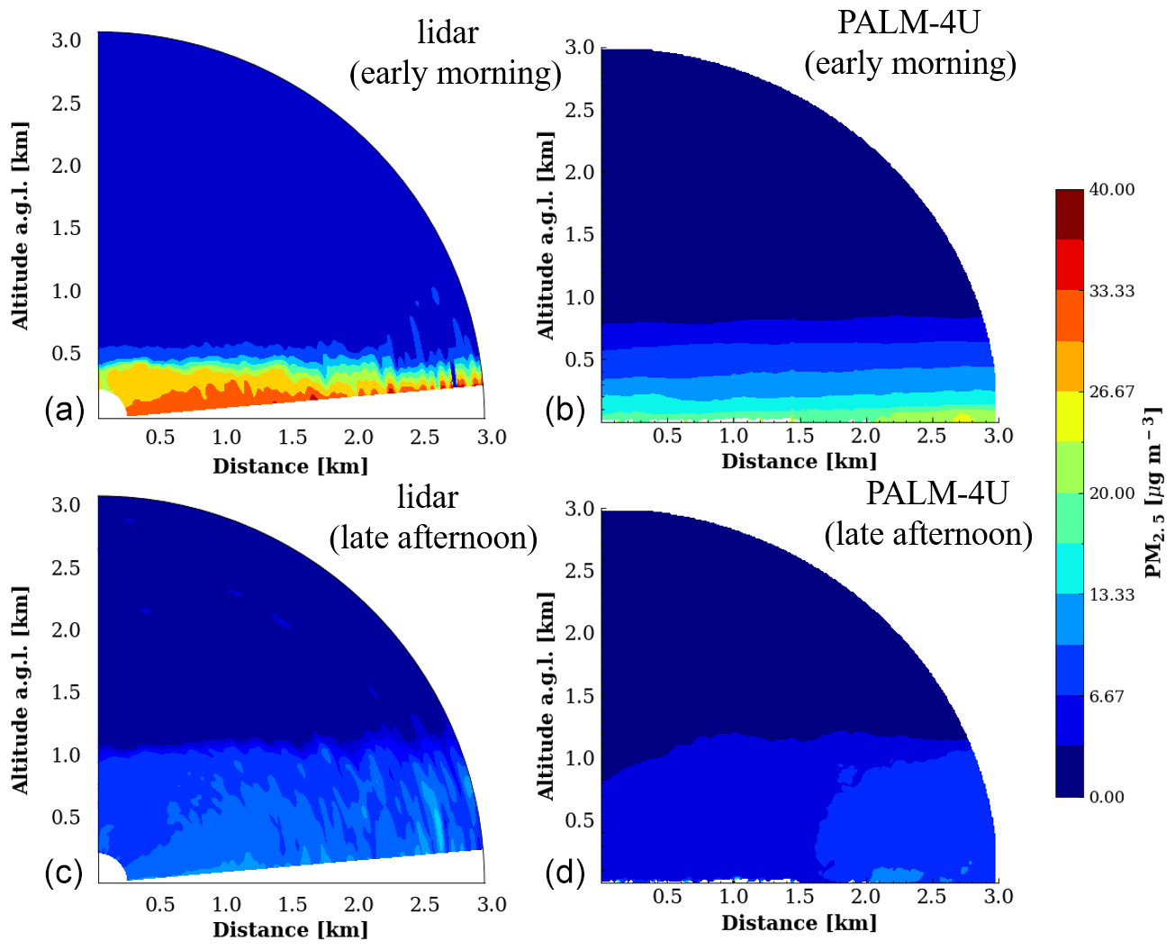
Figure 9Range–height cross section of PM2.5 concentrations from a scanning aerosol lidar (a, c) and the PALM-4U simulation (b, d) at two different periods on 14 February 2018 (a, b: 09:12–09:20 UTC (early morning); c, d: 16:07–16:15 UTC (later afternoon)).
Several factors of uncertainty contribute to this underestimation, namely emissions, transformation processes, and initial and lateral boundary conditions (ICs and LBCs). Residential emissions are not included in this simulation, which we expect to be a significant source in winter. Furthermore, traffic emissions are parameterized based on street type and time of day (Khan et al., 2021). These very simple assumptions cannot accurately simulate the true emissions, especially if traffic congestion amplifies true emissions. High levels of HOA (traffic related aerosol) were identified in the PMF analysis of organic aerosol, as shown in Fig. 4c, which substantiates the assumption that this is a large source of uncertainty in our simulation. Finally, the IC and LBC for this simulations were based on the nocturnal profile on 14 February 2018 at 00:00 UTC. Providing spatially and temporally variable IC and LBC would most likely improve agreement of the regional background concentrations and allow us to disentangle this contribution to the total uncertainty from the local emissions. We found that the large distance from the outer domain boundary to the inner domain boundary (> 3 BLH during daytime) allowed sufficient “spin-up” mixing upstream of the child domain, such that turbulence and vertical distribution behaved plausibly. Depending on the grid spacing of 40 m, the spatial heterogeneity transported into the child domain was however quite diffuse, as expected. It is also noteworthy that only road emissions, transport, and dry deposition were simulated here. Particulate processes like aggregation, wet deposition, chemical transformation or secondary aerosol formation are not accounted for, with the underlying assumption being that on local scales and 24 h timescales, primary emissions and transport are more dominant. As mentioned in the Introduction, 58 % of the PM10 has been attributed to road emissions (Leiber et al., 2016). This being an annual average, the omission of residential heating emissions most likely accounts for a large fraction of the simulated underestimation during this cold winter period. Additionally, most smaller roads are not fully represented in the parent domain with 40 m grid spacing, such that the regional urban background road emissions might be underrepresented with contributions only from highways and other large road structures. This is substantiated by our finding that HOA is dominant in these periods, as shown in Fig. 4d.
Figure 9 shows a range–height cross section of PM2.5 concentrations derived from lidar measurements and the PALM-4U simulation during two different periods (09:12–09:20; 16:07–16:15 UTC) on 14 February 2018. As we already know that the PALM-4U underestimated the PM2.5 concentrations by a factor of 4.5 ± 2.1, we scaled up the PM2.5 concentrations from the PALM-4U simulation by a factor of 4.5 to better demonstrate aerosol spatial distribution. The figure panels in the first row demonstrate the aerosol spatial distribution in the early morning, which reflect a similar shallow boundary layer and high ground-level aerosol loading. The figure panels in the second row show the aerosol spatial distribution in the afternoon, which reflects a well-mixed boundary layer and relatively low-concentration and homogeneous aerosol distributions. Compared with the observational data, PALM-4U simulated the aerosol spatial distribution and boundary layer structure well. However, there is still some inconsistency that needs to be cleared up. Compared to observational data, the model shows more homogeneous spatial and temporal aerosol distribution, especially for the case in the afternoon, as shown in the second row of Fig. 9. One possible reason for this inconsistency is that the PALM-4U did not resolve all turbulent eddies (i.e. limited by 10 m grid spacing) as stable winter conditions might require finer grid spacings. The lack of spatial and temporal detail in the emissions also contributes to the diffuse characteristic of the simulated concentration fields. Another reason for this lack of structure could be associated with the time averaging; 10 min might be long enough to blur many small-scale instantaneous structures that the instrument might detect in a scan.
This study investigates boundary layer dynamics and air quality in a complex terrain by combining a scanning aerosol lidar, a wind lidar, a microwave radiometer, different in situ aerosol characterization instruments, radiosondes, and a large eddy simulation for downtown Stuttgart in winter. The boundary layer heights retrieved from lidar show good agreement with those from radiosondes, with a slope of 1.102 ± 0.135 and a Pearson correlation coefficient of 0.86, respectively. This agreement reflects the good quality of our measurements and retrieval algorithms. Stagnant meteorological patterns with strong temperature inversion and low wind speeds can cause an accumulation of aerosol at ground level, contributing to significant air pollution events, similar to previous observations in other cities (Jia et al., 2021; J. Li et al., 2021; Huang et al., 2018).
Ground-level aerosol concentrations are anti-correlated with mixing layer heights but are correlated with stable boundary layer heights in the later night and early morning as reported by Yuval et al. (2020) and Lou et al. (2019). The anti-correlation indicates that the convection within the boundary layer can dilute ground-level aerosol, whereas the correlation means that this relationship is not only affected by boundary layer mixing process but also by local aerosol emissions (Huang et al., 2023; Tsai et al., 2011).
Two selected cases show that the evolution of boundary layer structures was affected by solar irradiation, clouds, temperature, and wind and is very different under different meteorological conditions (Cao et al., 2020; Y. Li et al., 2021). Cloud cover during previous night-time can significantly weaken the temperature inversion, potentially causing a faster increase in boundary layer heights after sunrise. This is especially important for aerosol dilution during the morning rush hour and demonstrates how strong different meteorological aspects influence air quality levels.
Although the investigated time period is relatively short, the correlation between the boundary layer and aerosol distribution revealed by this dataset fitted well with a 2-year dataset, which supports the robustness of our results. Furthermore, the meteorological conditions during the measurement period can be considered quite typical winter conditions under the influence of a high-pressure system. Therefore, our results have sufficient representativeness to compare with, for example, other seasons.
The comparison of PALM-4U model results with observational data shows that the simulated boundary layer dynamics and aerosol mixing and transport processes are described relatively well by PALM-4U. However, it underestimates the PM2.5 concentrations by a factor of 4.5 ± 2.1. This underestimation is mainly due to uncertainties of emissions as well as initial and lateral boundary conditions (ICs and LBCs) (Khan et al., 2021; Maronga et al., 2020). Although the simulated aerosol concentrations are systematically lower than the observation values, the PALM-4U model still successfully reproduced the boundary layer evolution and its mixing effect on the ground-level aerosol. This helps to better understand the boundary layer dynamics and the aerosol dispersion paths within the boundary layer.
PALM-4U model validation has been conducted at different places in terms of meteorological parameters as well as gas and particle pollutants (e.g. Oklahoma, USA; Münster, Germany; Prague, Czech Republic; Berlin, Germany; Ōtautahi / Christchurch, Aotearoa / New Zealand; Hong Kong SAR, China; Dresden, Germany) (Tewari et al., 2010; Paas et al., 2020; Resler et al., 2021; Khan et al., 2021; Lin et al., 2021; Wang et al., 2023). However, our research aims to contribute additional insights by focusing on the validation of boundary layer dynamics and aerosol mixing and transport processes within the boundary layer in stable winter conditions. This work presents one of the first winter evaluations of PALM-4U in simulating aerosol distributions in a complex basin-like urban area. This study contributes to characterizing the structure of the urban boundary layer in complex terrain and understanding the processes of air pollution in downtown Stuttgart. The impact of local emissions from different sources as well as horizontal and vertical transport can be distinguished based on this work. This is helpful to understand the influence of boundary layer mixing on aerosol evolution and to improve air quality predictions and mitigation measures in urban areas with complex topography.
Furthermore, leveraging comprehensive observed data and high-resolution simulations from model outputs enables the reproduction of urban scenarios at the street level, which will contribute to advancement of the development of a digital twin for urban climates in the future (Chen et al., 2023; Schrotter and Hürzeler, 2020; Caprari et al., 2022).
Regarding future work related to this study, this model version did not consider the aerosol chemical composition, and only PM2.5 and PM10 were predicted via prognostic scalar transport equations. Hence, the formation of secondary aerosol generated by chemical reactions is not considered in this work, and it would be the next step of our work to include this. In the scope of this study we did not have computational resources and personnel to set up and test a full SALSA aerosol physics simulation. Given that we attempted the first winter evaluation of PALM's aerosol simulation behaviour in complex urban terrain, our objective was to mostly check for plausible boundary layer dynamics and spatial patterns. More research is needed with more resources to address this in detail. Also, we acknowledge that the current utilization of the model is somewhat limited, and we are aware of the substantial potential of the PALM-4U model for a more detailed comparison with our comprehensive observations. For instance, we plan to conduct sensitivity tests on the impact of clouds on boundary layer evolution, on aerosol mixing processes, and on aerosol physical and chemical transformation processes. Finally, in an upcoming study we aim to present more details of the model simulations in the context of different dynamic processes. Nonetheless, we think it is useful to demonstrate the actual model capabilities in comparison with these excellent observational data since there are currently very few PALM-4U applications with aerosols.
The code used to analyze the lidar data is the property of Raymetrics, but we have shown that it gives the same results as the code Single Calculus Chain (SCC) provided by EARLINET at https://www.earlinet.org/index.php?id=281 (D'Amico et al., 2015; https://scc.imaa.cnr.it/, last access: 4 June 2024, login required) and publicly available. The code of the PALM-4U model can be found on the PALM website (https://gitlab.palm-model.org/releases/palm_model_system, PALM group, 2024).
The lidar data and in situ measurement data are available via the open-access data repository KITopen (https://doi.org/10.35097/vbjzahy9ej4c1b69, Zhang et al., 2024). The radiosonde data are available upon request from the data originator (DWD; datenservice@dwd.de). The palm simulation data are available upon request from the data originator (christopher.holst@kit.edu).
The supplement related to this article is available online at: https://doi.org/10.5194/acp-24-10617-2024-supplement.
HS, XS, and WH performed the measurements. HZ analysed the scanning lidar data and combined all available data together. OK analysed radiosonde, wind lidar, and temperature lidar data. CCH and BK performed and analysed the WRF and PALM-4U simulations and wrote the corresponding parts of the manuscript. HZ wrote the manuscript with support from HS as well as contributions from all co-authors.
At least one of the (co-)authors is a member of the editorial board of Atmospheric Chemistry and Physics. The peer-review process was guided by an independent editor, and the authors also have no other competing interests to declare.
Publisher's note: Copernicus Publications remains neutral with regard to jurisdictional claims made in the text, published maps, institutional affiliations, or any other geographical representation in this paper. While Copernicus Publications makes every effort to include appropriate place names, the final responsibility lies with the authors.
We acknowledge the technical staff of the Institute of Meteorology and Climate Research and German weather service (DWD), especially Anderas Wieser and Bianca Adler, for their support with wind lidar and microwave radiometer data collection. Financial support was provided by the project Modular Observation Solutions for Earth Systems (MOSES) of the Helmholtz Association (HGF) and the German Federal Ministry of Education and Research (BMBF) under grants 01LP1602 G and 01LP1602 K within the research programme [UC]2. Financial support was also provided by the Horizon 2020 Framework Programme of the European Research Council (CHAPAs, grant no. 850614). This work was supported by the North German Supercomputing Alliance (HLRN). We are grateful to the HLRN supercomputer staff, especially Stefan Wollny for his continual help and support.
This research has been supported by the Helmholtz-Zentrum für Umweltforschung (grant no. 871128), the Bundesministerium für Bildung und Forschung (grant nos. 01LP1602 G and 01LP1602 K), and the EU H2020 European Research Council (grant no. 850614).
The article processing charges for this open-access publication were covered by the Karlsruhe Institute of Technology (KIT).
This paper was edited by Andreas Petzold and reviewed by I. Pérez and one anonymous referee.
Ackerman, A. S., Kirkpatrick, M. P., Stevens, D. E., and Toon, O. B.: The impact of humidity above stratiform clouds on indirect aerosol climate forcing, Nature, 432, 1014–1017, https://doi.org/10.1038/nature03174, 2004. a
Aljawhary, D., Lee, A. K. Y., and Abbatt, J. P. D.: High-resolution chemical ionization mass spectrometry (ToF-CIMS): application to study SOA composition and processing, Atmos. Meas. Tech., 6, 3211–3224, https://doi.org/10.5194/amt-6-3211-2013, 2013. a
Avdikos, G.: Powerful Raman Lidar systems for atmospheric analysis and high-energy physics experiments, EPJ Web Conf., 89, 04003, https://doi.org/10.1051/epjconf/20158904003, 2015. a
Bates, T. S., Quinn, P. K., Covert, D. S., Coffman, D. J., Johnson, J. E., and Wiedensohler, A.: Aerosol physical properties and processes in the lower marine boundary layer: A comparison of shipboard sub-micron data from ACE-1 and ACE-2, Tellus B, 52, 258–272, https://doi.org/10.1034/j.1600-0889.2000.00021.x, 2000. a
Bates, T. S., Coffman, D. J., Covert, D. S., and Quinn, P. K.: Regional marine boundary layer aerosol size distributions in the Indian, Atlantic, and Pacific Oceans: A comparison of INDOEX measurements with ACE-1, ACE-2, and Aerosols99, J. Geophys. Res.-Atmos., 107, INX2–25, https://doi.org/10.1029/2001JD001174, 2002. a
Canonaco, F., Crippa, M., Slowik, J. G., Baltensperger, U., and Prévôt, A. S. H.: SoFi, an IGOR-based interface for the efficient use of the generalized multilinear engine (ME-2) for the source apportionment: ME-2 application to aerosol mass spectrometer data, Atmos. Meas. Tech., 6, 3649–3661, https://doi.org/10.5194/amt-6-3649-2013, 2013. a
Cao, B., Wang, X., Ning, G., Yuan, L., Jiang, M., Zhang, X., and Wang, S.: Factors influencing the boundary layer height and their relationship with air quality in the Sichuan Basin, China, Sci. Total Environ., 727, 138584, https://doi.org/10.1016/j.scitotenv.2020.138584, 2020. a
Caprari, G., Castelli, G., Montuori, M., Camardelli, M., and Malvezzi, R.: Digital Twin for Urban Planning in the Green Deal Era: A State of the Art and Future Perspectives, Sustainability, 14, 6263, https://doi.org/10.3390/su14106263, 2022. a
Chan, C. K. and Yao, X.: Air pollution in mega cities in China, Atmos. Environ., 42, 1–42, https://doi.org/10.1016/j.atmosenv.2007.09.003, 2008. a
Chen, B., Lin, C., Gong, P., and An, J.: Optimize urban shade using digital twins of cities, Nature, 622, 242–242, https://doi.org/10.1038/d41586-023-03189-x, 2023. a
Crippa, M., Canonaco, F., Lanz, V. A., Äijälä, M., Allan, J. D., Carbone, S., Capes, G., Ceburnis, D., Dall'Osto, M., Day, D. A., DeCarlo, P. F., Ehn, M., Eriksson, A., Freney, E., Hildebrandt Ruiz, L., Hillamo, R., Jimenez, J. L., Junninen, H., Kiendler-Scharr, A., Kortelainen, A.-M., Kulmala, M., Laaksonen, A., Mensah, A. A., Mohr, C., Nemitz, E., O'Dowd, C., Ovadnevaite, J., Pandis, S. N., Petäjä, T., Poulain, L., Saarikoski, S., Sellegri, K., Swietlicki, E., Tiitta, P., Worsnop, D. R., Baltensperger, U., and Prévôt, A. S. H.: Organic aerosol components derived from 25 AMS data sets across Europe using a consistent ME-2 based source apportionment approach, Atmos. Chem. Phys., 14, 6159–6176, https://doi.org/10.5194/acp-14-6159-2014, 2014. a
D'Amico, G., Amodeo, A., Baars, H., Binietoglou, I., Freudenthaler, V., Mattis, I., Wandinger, U., and Pappalardo, G.: EARLINET Single Calculus Chain – overview on methodology and strategy, Atmos. Meas. Tech., 8, 4891–4916, https://doi.org/10.5194/amt-8-4891-2015, 2015 (code available at: https://www.earlinet.org/index.php?id=281, last access: 4 June 2024). a
DeCarlo, P. F., Ulbrich, I. M., Crounse, J., de Foy, B., Dunlea, E. J., Aiken, A. C., Knapp, D., Weinheimer, A. J., Campos, T., Wennberg, P. O., and Jimenez, J. L.: Investigation of the sources and processing of organic aerosol over the Central Mexican Plateau from aircraft measurements during MILAGRO, Atmos. Chem. Phys., 10, 5257–5280, https://doi.org/10.5194/acp-10-5257-2010, 2010. a
Demuzere, M., Argüeso, D., Zonato, A., and Kittner, J.: W2W: A Python package that injects WUDAPT's Local Climate Zone information in WRF, Journal of Open Source Software, 7, 4432, https://doi.org/10.21105/joss.04432, 2022a. a
Demuzere, M., Kittner, J., Martilli, A., Mills, G., Moede, C., Stewart, I. D., van Vliet, J., and Bechtel, B.: A global map of local climate zones to support earth system modelling and urban-scale environmental science, Earth Syst. Sci. Data, 14, 3835–3873, https://doi.org/10.5194/essd-14-3835-2022, 2022b. a
Dias-Júnior, C. Q., Carneiro, R. G., Fisch, G., D'Oliveira, F. A. F., Sörgel, M., Botía, S., Machado, L. A. T., Wolff, S., dos Santos, R. M. N., and Pöhlker, C.: Intercomparison of Planetary Boundary Layer Heights Using Remote Sensing Retrievals and ERA5 Reanalysis over Central Amazonia, Remote Sens.-Basel, 14, 4561, https://doi.org/10.3390/rs14184561, 2022. a
Floors, R., Vincent, C. L., Gryning, S.-E., Peña, A., and Batchvarova, E.: The wind profile in the coastal boundary layer: Wind lidar measurements and numerical modelling, Bound.-Lay. Meteorol., 147, 469–491, https://doi.org/10.1007/s10546-012-9791-9, 2013. a
Freudenthaler, V.: About the effects of polarising optics on lidar signals and the Δ90 calibration, Atmos. Meas. Tech., 9, 4181–4255, https://doi.org/10.5194/amt-9-4181-2016, 2016. a
Froidevaux, M., Higgins, C. W., Simeonov, V., Ristori, P., Pardyjak, E., Serikov, I., Calhoun, R., van den Bergh, H., and Parlange, M. B.: A Raman lidar to measure water vapor in the atmospheric boundary layer, Adv. Water Resour., 51, 345–356, https://doi.org/10.1016/j.advwatres.2012.04.008, 2013. a
Garratt, J.: Review: the atmospheric boundary layer, Earth-Sci. Rev., 37, 89–134, https://doi.org/10.1016/0012-8252(94)90026-4, 1994. a
Gentine, P., Chhang, A., Rigden, A., and Salvucci, G.: Evaporation estimates using weather station data and boundary layer theory, Geophys. Res. Lett., 43, 11661–11670, https://doi.org/10.1002/2016GL070819, 2016. a
Greenberg, J., Guenther, A., Zimmerman, P., Baugh, W., Geron, C., Davis, K., Helmig, D., and Klinger, L.: Tethered balloon measurements of biogenic VOCs in the atmospheric boundary layer, Atmos. Environ., 33, 855–867, https://doi.org/10.1016/S1352-2310(98)00302-1, 1999. a
Guo, J., Miao, Y., Zhang, Y., Liu, H., Li, Z., Zhang, W., He, J., Lou, M., Yan, Y., Bian, L., and Zhai, P.: The climatology of planetary boundary layer height in China derived from radiosonde and reanalysis data, Atmos. Chem. Phys., 16, 13309–13319, https://doi.org/10.5194/acp-16-13309-2016, 2016. a
Guo, J., Su, T., Li, Z., Miao, Y., Li, J., Liu, H., Xu, H., Cribb, M., and Zhai, P.: Declining frequency of summertime local-scale precipitation over eastern China from 1970 to 2010 and its potential link to aerosols, Geophys. Res. Lett., 44, 5700–5708, https://doi.org//10.1002/2017GL073533, 2017. a
Guo, J.-P., Zhang, X.-Y., Che, H.-Z., Gong, S.-L., An, X., Cao, C.-X., Guang, J., Zhang, H., Wang, Y.-Q., Zhang, X.-C., Xue, M., and Li, X.-W.: Correlation between PM concentrations and aerosol optical depth in eastern China, Atmos. Environ., 43, 5876–5886, https://doi.org/10.1016/j.atmosenv.2009.08.026, 2009. a, b
Hammann, E., Behrendt, A., Le Mounier, F., and Wulfmeyer, V.: Temperature profiling of the atmospheric boundary layer with rotational Raman lidar during the HD(CP)2 Observational Prototype Experiment, Atmos. Chem. Phys., 15, 2867–2881, https://doi.org/10.5194/acp-15-2867-2015, 2015. a
Hebbert, M., Webb, B., Gossop, C., and Nan, S.: Towards a Liveable Urban Climate: Lessons from Stuttgart, Routledge, United Kingdom, 132–150, ISBN: 978-0-415-50956-5, 2012. a
Heldens, W., Burmeister, C., Kanani-Sühring, F., Maronga, B., Pavlik, D., Sühring, M., Zeidler, J., and Esch, T.: Geospatial input data for the PALM model system 6.0: model requirements, data sources and processing, Geosci. Model Dev., 13, 5833–5873, https://doi.org/10.5194/gmd-13-5833-2020, 2020. a
Hennemuth, B. and Lammert-Stockschlaeder, A.: Determination of the Atmospheric Boundary Layer Height from Radiosonde and Lidar Backscatter, Bound.-Lay. Meteorol., 120, 181–200, https://doi.org/10.1007/s10546-005-9035-3, 2006. a, b
Hersbach, H., Bell, B., Berrisford, P., Hirahara, S., Horányi, A., Muñoz-Sabater, J., Nicolas, J., Peubey, C., Radu, R., Schepers, D., Simmons, A., Soci, C., Abdalla, S., Abellan, X., Balsamo, G., Bechtold, P., Biavati, G., Bidlot, J., Bonavita, M., De Chiara, G., Dahlgren, P., Dee, D., Diamantakis, M., Dragani, R., Flemming, J., Forbes, R., Fuentes, M., Geer, A., Haimberger, L., Healy, S., Hogan, R. J., Hólm, E., Janisková, M., Keeley, S., Laloyaux, P., Lopez, P., Lupu, C., Radnoti, G., de Rosnay, P., Rozum, I., Vamborg, F., Villaume, S., and Thépaut, J.-N.: The ERA5 global reanalysis, Q. J. Roy. Meteor. Soc., 146, 1999–2049, https://doi.org/10.1002/qj.3803, 2020. a, b
Huang, Q., Cai, X., Wang, J., Song, Y., and Zhu, T.: Climatological study of the Boundary-layer air Stagnation Index for China and its relationship with air pollution, Atmos. Chem. Phys., 18, 7573–7593, https://doi.org/10.5194/acp-18-7573-2018, 2018. a, b, c
Huang, W., Saathoff, H., Shen, X., Ramisetty, R., Leisner, T., and Mohr, C.: Seasonal characteristics of organic aerosol chemical composition and volatility in Stuttgart, Germany, Atmos. Chem. Phys., 19, 11687–11700, https://doi.org/10.5194/acp-19-11687-2019, 2019. a, b, c, d, e
Huang, X., Wang, Y., Shang, Y., Song, X., Zhang, R., Wang, Y., Li, Z., and Yang, Y.: Contrasting the effect of aerosol properties on the planetary boundary layer height in Beijing and Nanjing, Atmos. Environ., 308, 119861, https://doi.org/10.1016/j.atmosenv.2023.119861, 2023. a, b
Ji, D., Li, L., Wang, Y., Zhang, J., Cheng, M., Sun, Y., Liu, Z., Wang, L., Tang, G., Hu, B., Chao, N., Wen, T., and Miao, H.: The heaviest particulate air-pollution episodes occurred in northern China in January, 2013: Insights gained from observation, Atmos. Environ., 92, 546–556, https://doi.org/10.1016/j.atmosenv.2014.04.048, 2014. a
Jia, W., Zhang, X., Wang, J., Yang, Y., and Zhong, J.: The influence of stagnant and transport types weather on heavy pollution in the Yangtze-Huaihe valley, China, Sci. Total Environ., 792, 148393, https://doi.org//10.1016/j.scitotenv.2021.148393, 2021. a
Jordan, A., Haidacher, S., Hanel, G., Hartungen, E., Märk, L., Seehauser, H., Schottkowsky, R., Sulzer, P., and Märk, T.: A high resolution and high sensitivity proton-transfer-reaction time-of-flight mass spectrometer (PTR-TOF-MS), Int. J. Mass Spectrom., 286, 122–128, https://doi.org/10.1016/j.ijms.2009.07.005, 2009. a
Katsoulis, B.: Some meteorological aspects of air pollution in Athens, Greece, Meteorol. Atmos. Phys., 39, 203–212, https://doi.org/10.1007/BF01030298, 1988. a
Khan, B., Banzhaf, S., Chan, E. C., Forkel, R., Kanani-Sühring, F., Ketelsen, K., Kurppa, M., Maronga, B., Mauder, M., Raasch, S., Russo, E., Schaap, M., and Sühring, M.: Development of an atmospheric chemistry model coupled to the PALM model system 6.0: implementation and first applications, Geosci. Model Dev., 14, 1171–1193, https://doi.org/10.5194/gmd-14-1171-2021, 2021. a, b, c, d
Kiehl, J. T. and Briegleb, B. P.: The Relative Roles of Sulfate Aerosols and Greenhouse Gases in Climate Forcing, Science, 260, 311–314, https://doi.org/10.1126/science.260.5106.311, 1993. a
Kim, M.-S. and Kwon, B. H.: Estimation of sensible heat flux and atmospheric boundary layer height using an unmanned aerial vehicle, Atmosphere, 10, 363, https://doi.org/10.3390/atmos10070363, 2019. a
Kiseleva, O., Kalthoff, N., Adler, B., Kossmann, M., Wieser, A., and Rinke, R.: Nocturnal atmospheric conditions and their impact on air pollutant concentrations in the city of Stuttgart, Meteorol. Appl., 28, e2037, https://doi.org/10.1002/met.2037, 2021. a
Kiseleva, O., Gantner, L., Kalthoff, N., Kossmann, M., and Holst, C.: Evaluation of the Urban Climate Model PALM-4U over Hilly Terrain Using Wind and Turbulence Observations, Meteorol. Z., 33, 177–198, https://doi.org/10.1127/metz/2024/1193, 2024. a, b
Kokkola, H., Korhonen, H., Lehtinen, K. E. J., Makkonen, R., Asmi, A., Järvenoja, S., Anttila, T., Partanen, A.-I., Kulmala, M., Järvinen, H., Laaksonen, A., and Kerminen, V.-M.: SALSA – a Sectional Aerosol module for Large Scale Applications, Atmos. Chem. Phys., 8, 2469–2483, https://doi.org/10.5194/acp-8-2469-2008, 2008. a
Kokkola, H., Kühn, T., Laakso, A., Bergman, T., Lehtinen, K. E. J., Mielonen, T., Arola, A., Stadtler, S., Korhonen, H., Ferrachat, S., Lohmann, U., Neubauer, D., Tegen, I., Siegenthaler-Le Drian, C., Schultz, M. G., Bey, I., Stier, P., Daskalakis, N., Heald, C. L., and Romakkaniemi, S.: SALSA2.0: The sectional aerosol module of the aerosol–chemistry–climate model ECHAM6.3.0-HAM2.3-MOZ1.0, Geosci. Model Dev., 11, 3833–3863, https://doi.org/10.5194/gmd-11-3833-2018, 2018. a
Kurppa, M., Hellsten, A., Roldin, P., Kokkola, H., Tonttila, J., Auvinen, M., Kent, C., Kumar, P., Maronga, B., and Järvi, L.: Implementation of the sectional aerosol module SALSA2.0 into the PALM model system 6.0: model development and first evaluation, Geosci. Model Dev., 12, 1403–1422, https://doi.org/10.5194/gmd-12-1403-2019, 2019. a, b
Lenschow, D. H. (Ed.): Aircraft measurements in the boundary layer, in: Probing the atmospheric boundary layer, Springer, 39–55, https://doi.org/10.1007/978-1-944970-14-7_5, 1986. a
Li, J., Li, C., Zhao, C., and Su, T.: Changes in surface aerosol extinction trends over China during 1980–2013 inferred from quality-controlled visibility data, Geophys. Res. Lett., 43, 8713–8719, https://doi.org/10.1002/2016GL070201, 2016. a
Li, J., Gao, W., Cao, L., He, L., Zhang, X., Yan, Y., Mao, J., Xin, J., Wang, L., Tang, G., Liu, Z., Ji, D., Hu, B., Zhao, D., Zhao, S., Jia, D., and Wang, Y.: Effects of different stagnant meteorological conditions on aerosol chemistry and regional transport changes in Beijing, China, Atmos. Environ., 258, 118483, https://doi.org/10.1016/j.atmosenv.2021.118483, 2021. a
Li, Y., Li, J., Zhao, Y., Lei, M., Zhao, Y., Jian, B., Zhang, M., and Huang, J.: Long-term variation of boundary layer height and possible contribution factors: A global analysis, Sci. Total Environ., 796, 148950, https://doi.org/10.1016/j.scitotenv.2021.148950, 2021. a
Li, Z., Guo, J., Ding, A., Liao, H., Liu, J., Sun, Y., Wang, T., Xue, H., Zhang, H., and Zhu, B.: Aerosol and boundary-layer interactions and impact on air quality, Natl. Sci. Rev., 4, 810–833, https://doi.org/10.1093/nsr/nwx117, 2017. a, b
Lin, D., Khan, B., Katurji, M., Bird, L., Faria, R., and Revell, L. E.: WRF4PALM v1.0: a mesoscale dynamical driver for the microscale PALM model system 6.0, Geosci. Model Dev., 14, 2503–2524, https://doi.org/10.5194/gmd-14-2503-2021, 2021. a
Liu, S. and Liang, X.-Z.: Observed diurnal cycle climatology of planetary boundary layer height, J. Climate, 23, 5790–5809, https://doi.org/10.1175/2010JCLI3552.1, 2010. a
Löhnert, U. and Maier, O.: Operational profiling of temperature using ground-based microwave radiometry at Payerne: prospects and challenges, Atmos. Meas. Tech., 5, 1121–1134, https://doi.org/10.5194/amt-5-1121-2012, 2012. a
Lou, M., Guo, J., Wang, L., Xu, H., Chen, D., Miao, Y., Lv, Y., Li, Y., Guo, X., Ma, S., and Li, J.: On the relationship between aerosol and boundary layer height in summer in China under different thermodynamic conditions, Earth and Space Science, 6, 887–901, https://doi.org/10.1029/2019EA000620, 2019. a
LUBW: Office for Environmental Protection: Luft: Erfolgreiche Maßnahmen zur Luftreinhaltung in Stuttgart, https://www.stuttgart.de/leben/umwelt/luft/ (last accessed: 18 February 2022), 2016. a
Leiber, T., Scheu-Hachtel, H., Graf, T., Scheinhardt, S., and Wirth, R.: Luft: Erfolgreiche Maßnahmen zur Luftreinhaltung in Stuttgart, Office for Environmental Protection, https://pudi.lubw.de/detailseite/-/publication/37937 (last accessed: 14 September 2024), 2016. a, b
Maronga, B., Banzhaf, S., Burmeister, C., Esch, T., Forkel, R., Fröhlich, D., Fuka, V., Gehrke, K. F., Geletič, J., Giersch, S., Gronemeier, T., Groß, G., Heldens, W., Hellsten, A., Hoffmann, F., Inagaki, A., Kadasch, E., Kanani-Sühring, F., Ketelsen, K., Khan, B. A., Knigge, C., Knoop, H., Krč, P., Kurppa, M., Maamari, H., Matzarakis, A., Mauder, M., Pallasch, M., Pavlik, D., Pfafferott, J., Resler, J., Rissmann, S., Russo, E., Salim, M., Schrempf, M., Schwenkel, J., Seckmeyer, G., Schubert, S., Sühring, M., von Tils, R., Vollmer, L., Ward, S., Witha, B., Wurps, H., Zeidler, J., and Raasch, S.: Overview of the PALM model system 6.0, Geosci. Model Dev., 13, 1335–1372, https://doi.org/10.5194/gmd-13-1335-2020, 2020. a, b, c, d, e, f
Mason, P. J.: Large-eddy simulation of the convective atmospheric boundary layer, J. Atmos. Sci., 46, 1492–1516, https://doi.org/10.1175/1520-0469(1989)046<1492:LESOTC>2.0.CO;2, 1989. a
Mayer, H.: Air pollution in cities, Atmos. Environ., 33, 4029–4037, https://doi.org/10.1016/S1352-2310(99)00144-2, 1999. a
Medeiros, B., Hall, A., and Stevens, B.: What controls the mean depth of the PBL?, J. Climate, 18, 3157–3172, https://doi.org/10.1175/JCLI3417.1, 2005. a
Mohr, C., DeCarlo, P. F., Heringa, M. F., Chirico, R., Slowik, J. G., Richter, R., Reche, C., Alastuey, A., Querol, X., Seco, R., Peñuelas, J., Jiménez, J. L., Crippa, M., Zimmermann, R., Baltensperger, U., and Prévôt, A. S. H.: Identification and quantification of organic aerosol from cooking and other sources in Barcelona using aerosol mass spectrometer data, Atmos. Chem. Phys., 12, 1649–1665, https://doi.org/10.5194/acp-12-1649-2012, 2012. a
Nash, D. G., Baer, T., and Johnston, M. V.: Aerosol mass spectrometry: An introductory review, Int. J. Mass Spectrom., 258, 2–12, https://doi.org/10.1016/j.ijms.2006.09.017, 2006. a
Neff, W., Helmig, D., Grachev, A., and Davis, D.: A study of boundary layer behavior associated with high NO concentrations at the South Pole using a minisodar, tethered balloon, and sonic anemometer, Atmos. Environ., 42, 2762–2779, https://doi.org/10.1016/j.atmosenv.2007.01.033, 2008. a, b
Paas, B., Zimmermann, T., and Klemm, O.: Analysis of a turbulent wind field in a street canyon: Good agreement between LES model results and data from a mobile platform, Meteorol. Z., 30, 45–57, https://doi.org/10.1127/metz/2020/1006, 2020. a
Paatero, P.: Least squares formulation of robust non-negative factor analysis, Chemometr. Intell. Lab., 37, 23–35, https://doi.org/10.1016/S0169-7439(96)00044-5, 1997. a
Paatero, P. and Tapper, U.: Positive matrix factorization: A non-negative factor model with optimal utilization of error estimates of data values, Environmetrics, 5, 111–126, https://doi.org/10.1002/env.3170050203, 1994. a
Pal, S., Behrendt, A., and Wulfmeyer, V.: Elastic-backscatter-lidar-based characterization of the convective boundary layer and investigation of related statistics, Ann. Geophys., 28, 825–847, https://doi.org/10.5194/angeo-28-825-2010, 2010. a
PALM group: PALM model system, GitLab [code], https://gitlab.palm-model.org/releases/palm_model_system, last access: 14 September 2024. a
Petzold, A., Ogren, J. A., Fiebig, M., Laj, P., Li, S.-M., Baltensperger, U., Holzer-Popp, T., Kinne, S., Pappalardo, G., Sugimoto, N., Wehrli, C., Wiedensohler, A., and Zhang, X.-Y.: Recommendations for reporting “black carbon” measurements, Atmos. Chem. Phys., 13, 8365–8379, https://doi.org/10.5194/acp-13-8365-2013, 2013. a
Pöschl, U.: Atmospheric aerosols: composition, transformation, climate and health effects, Angew. Chem. Int. Edit., 44, 7520–7540, https://doi.org/10.1002/anie.200501122, 2005. a
Prabha, T. V., Venkatesan, R., Mursch-Radlgruber, E., Rengarajan, G., and Jayanthi, N.: Thermal internal boundary layer characteristics at a tropical coastal site as observed by a mini-SODAR under varying synoptic conditions, J. Earth Syst. Sci., 111, 63–77, https://doi.org/10.1007/BF02702223, 2002. a
Quan, J., Gao, Y., Zhang, Q., Tie, X., Cao, J., Han, S., Meng, J., Chen, P., and Zhao, D.: Evolution of planetary boundary layer under different weather conditions, and its impact on aerosol concentrations, Particuology, 11, 34–40, https://doi.org/10.1016/j.partic.2012.04.005, 2013. a, b
Raasch, S. and Schröter, M.: PALM – A large-eddy simulation model performing on massively parallel computers, Meteorol. Z., 10, 363–372, https://doi.org/10.1127/0941-2948/2001/0010-0363, 2001. a
Ramanathan, V., Crutzen, P. J., Kiehl, J., and Rosenfeld, D.: Aerosols, climate, and the hydrological cycle, Science, 294, 2119–2124, https://doi.org/10.1126/science.1064034, 2001. a
Rao, I. S., Anandan, V., and Reddy, P. N.: Evaluation of DBS wind measurement technique in different beam configurations for a VHF wind profiler, J. Atmos. Ocean. Tech., 25, 2304–2312, https://doi.org/10.1175/2008JTECHA1113.1, 2008. a
Reineman, B. D., Lenain, L., and Melville, W. K.: The use of ship-launched fixed-wing UAVs for measuring the marine atmospheric boundary layer and ocean surface processes, J. Atmos. Ocean. Tech., 33, 2029–2052, https://doi.org/10.1175/JTECH-D-15-0019.1, 2016. a
Resler, J., Eben, K., Geletič, J., Krč, P., Rosecký, M., Sühring, M., Belda, M., Fuka, V., Halenka, T., Huszár, P., Karlický, J., Benešová, N., Ďoubalová, J., Honzáková, K., Keder, J., Nápravníková, Š., and Vlček, O.: Validation of the PALM model system 6.0 in a real urban environment: a case study in Dejvice, Prague, the Czech Republic, Geosci. Model Dev., 14, 4797–4842, https://doi.org/10.5194/gmd-14-4797-2021, 2021. a
Samad, A. and Vogt, U.: Assessing the Effect of Traffic Density and Cold Airflows on the Urban Air Quality of a City with Complex Topography Using Continuous Measurements, Modern Environmental Science and Engineering, 6, 529–541, https://doi.org/10.15341/mese(2333-2581)/05.06.2020/002, 2020. a
Samad, A., Kiseleva, O., Holst, C. C., Wegener, R., Kossmann, M., Meusel, G., Fiehn, A., Erbertseder, T., Becker, R., Roiger, A., Stanislawsky, P., Klemp, D., Emeis, S., Kalthoff, N., and Vogt, U.: Meteorological and air quality measurements in a city region with complex terrain: influence of meteorological phenomena on urban climate, Meteorol. Z., 32, 293–315, https://doi.org/10.1127/metz/2023/1124, 2023. a
Schrotter, G. and Hürzeler, C.: The digital twin of the city of Zurich for urban planning, PFG–Journal of Photogrammetry, Remote Sensing and Geoinformation Science, 88, 99–112, https://doi.org/10.1007/s41064-020-00092-2, 2020. a
Schwartz, J., Spix, C., Wichmann, H., and Malin, E.: Air pollution and acute respiratory illness in five german communities, Environ. Res., 56, 1–14, https://doi.org/10.1016/S0013-9351(05)80104-5, 1991. a, b
Seidel, D. J., Ao, C. O., and Li, K.: Estimating climatological planetary boundary layer heights from radiosonde observations: Comparison of methods and uncertainty analysis, J. Geophys. Res.-Atmos., 115, D16113, https://doi.org/10.1029/2009JD013680, 2010. a
Shen, X., Vogel, H., Vogel, B., Huang, W., Mohr, C., Ramisetty, R., Leisner, T., Prévôt, A. S. H., and Saathoff, H.: Composition and origin of PM2.5 aerosol particles in the upper Rhine valley in summer, Atmos. Chem. Phys., 19, 13189–13208, https://doi.org/10.5194/acp-19-13189-2019, 2019. a
Shin, D. H., Müller, D., Choi, T., Noh, Y. M., Yoon, Y. J., Lee, K. H., Shin, S. K., Chae, N., Kim, K., and Kim, Y. J.: Influence of wind speed on optical properties of aerosols in the marine boundary layer measured by ship-borne DePolarization Lidar in the coastal area of Korea, Atmos. Environ., 83, 282–290, https://doi.org/10.1016/j.atmosenv.2013.10.027, 2014. a
Shiraiwa, M., Ueda, K., Pozzer, A., Lammel, G., Kampf, C. J., Fushimi, A., Enami, S., Arangio, A. M., Fröhlich-Nowoisky, J., Fujitani, Y., Furuyama, A., Lakey, P. S. J., Lelieveld, J., Lucas, K., Morino, Y., Pöschl, U., Takahama, S., Takami, A., Tong, H., Weber, B., Yoshino, A., and Sato, K.: Aerosol Health Effects from Molecular to Global Scales, Environ. Sci. Technol., 51, 13545–13567, https://doi.org/10.1021/acs.est.7b04417, 2017. a
Skamarock, W. C., Klemp, J. B., Dudhia, J., Gill, D. O., Liu, Z., Berner, J., Wang, W., Powers, J. G., Duda, M. G., Barker, D., and Huang, X.: A Description of the Advanced Research WRF Model Version 4.3, NCAR/TN-556+STR, https://doi.org/10.5065/1dfh-6p97, 2021. a
Slater, J., Tonttila, J., McFiggans, G., Connolly, P., Romakkaniemi, S., Kühn, T., and Coe, H.: Using a coupled large-eddy simulation–aerosol radiation model to investigate urban haze: sensitivity to aerosol loading and meteorological conditions, Atmos. Chem. Phys., 20, 11893–11906, https://doi.org/10.5194/acp-20-11893-2020, 2020. a
Song, J., Saathoff, H., Gao, L., Gebhardt, R., Jiang, F., Vallon, M., Bauer, J., Norra, S., and Leisner, T.: Variations of PM2.5 sources in the context of meteorology and seasonality at an urban street canyon in Southwest Germany, Atmos. Environ., 282, 119147, https://doi.org/10.1016/j.atmosenv.2022.119147, 2022. a, b
Spiga, A., Murdoch, N., Lorenz, R., Forget, F., Newman, C., Rodriguez, S., Pla-Garcia, J., Moreiras, D. V., Banfield, D., Perrin, C., Mueller, N. T., Lemmon, M., Millour, E., and Banerdt, W. B.: A Study of Daytime Convective Vortices and Turbulence in the Martian Planetary Boundary Layer Based on Half-a-Year of InSight Atmospheric Measurements and Large-Eddy Simulations, Journal of Geophysical Research: Planets, 126, e2020JE006511, https://doi.org/10.1029/2020JE006511, 2021. a
Stanier, C. O., Khlystov, A. Y., and Pandis, S. N.: Ambient aerosol size distributions and number concentrations measured during the Pittsburgh Air Quality Study (PAQS), Atmos. Environ., 38, 3275–3284, https://doi.org/10.1016/j.atmosenv.2004.03.020, 2004. a
Stocker, T.: Climate change 2013: the physical science basis: Working Group I contribution to the Fifth assessment report of the Intergovernmental Panel on Climate Change, Cambridge University Press, https://doi.org/10.1017/CBO9781107415324, 2014. a
Stoll, R., Gibbs, J. A., Salesky, S. T., Anderson, W., and Calaf, M.: Large-eddy simulation of the atmospheric boundary layer, Bound.-Lay. Meteorol., 177, 541–581, https://doi.org/10.1007/s10546-020-00556-3, 2020. a
Stull, R. B.: An introduction to boundary layer meteorology, Vol. 13, Springer Science & Business Media, https://doi.org/10.1007/978-94-009-3027-8, 1988. a, b, c
Stull, R. B. and Eloranta, E. W.: Boundary layer experiment–1983, B. Am. Meteorol. Soc., 65, 450–456, https://doi.org/10.1175/1520-0477(1984)065<0450:BLE>2.0.CO;2, 1984. a
Su, T., Li, Z., and Kahn, R.: Relationships between the planetary boundary layer height and surface pollutants derived from lidar observations over China: regional pattern and influencing factors, Atmos. Chem. Phys., 18, 15921–15935, https://doi.org/10.5194/acp-18-15921-2018, 2018. a
Su, T., Li, Z., Li, C., Li, J., Han, W., Shen, C., Tan, W., Wei, J., and Guo, J.: The significant impact of aerosol vertical structure on lower atmosphere stability and its critical role in aerosol–planetary boundary layer (PBL) interactions, Atmos. Chem. Phys., 20, 3713–3724, https://doi.org/10.5194/acp-20-3713-2020, 2020. a
Süddeutsche Zeitung: Stuttgart löst als erste Stadt in Deutschland den Feinstaubalarm aus, http://www.sueddeutsche.de/panorama/luftverschmutzung-stuttgart-loest-als-erste-stadt-in-deutschland-feinstaubalarm-aus-1.2822775 (last accessed: 18 February 2022), 2016 (in German). a
Tewari, M., Kusaka, H., Chen, F., Coirier, W. J., Kim, S., Wyszogrodzki, A. A., and Warner, T. T.: Impact of coupling a microscale computational fluid dynamics model with a mesoscale model on urban scale contaminant transport and dispersion, Atmos. Res., 96, 656–664, https://doi.org/10.1016/j.atmosres.2010.01.006, 2010. a
Tsai, T.-C., Jeng, Y.-J., Chu, D. A., Chen, J.-P., and Chang, S.-C.: Analysis of the relationship between MODIS aerosol optical depth and particulate matter from 2006 to 2008, Atmos. Environ., 45, 4777–4788, https://doi.org/10.1016/j.atmosenv.2009.10.006, 2011. a, b
Ulbrich, I. M., Canagaratna, M. R., Zhang, Q., Worsnop, D. R., and Jimenez, J. L.: Interpretation of organic components from Positive Matrix Factorization of aerosol mass spectrometric data, Atmos. Chem. Phys., 9, 2891–2918, https://doi.org/10.5194/acp-9-2891-2009, 2009. a
Vaisala: Description of Wind cube lidar, Vaisala Inc., https://www.vaisala.com/en/wind-lidars/wind-energy/windcube (last access: 1 September 2022), 2021. a
Wang, Y., Ma, Y.-F., Muñoz-Esparza, D., Dai, J., Li, C. W. Y., Lichtig, P., Tsang, R. C.-W., Liu, C.-H., Wang, T., and Brasseur, G. P.: Coupled mesoscale–microscale modeling of air quality in a polluted city using WRF-LES-Chem, Atmos. Chem. Phys., 23, 5905–5927, https://doi.org/10.5194/acp-23-5905-2023, 2023. a, b
Weger, M. and Heinold, B.: Air pollution trapping in the Dresden Basin from gray-zone scale urban modeling, Atmos. Chem. Phys., 23, 13769–13790, https://doi.org/10.5194/acp-23-13769-2023, 2023. a
Westwater, E., Han, Y., Irisov, V., Leuskiy, V., Kadygrov, E., and Viazankin, S.: Remote sensing of boundary layer temperature profiles by a scanning 5 mm microwave radiometer and RASS: Comparison experiments, J. Atmos. Ocean. Tech., 16, 805–818, https://doi.org/10.1175/1520-0426(1999)016<0805:RSOBLT>2.0.CO;2, 1999. a
Williams, B. J., Jayne, J. T., Lambe, A. T., Hohaus, T., Kimmel, J. R., Sueper, D., Brooks, W., Williams, L. R., Trimborn, A. M., Martinez, R. E., Hayes, P. L., Jimenez, J. L., Kreisberg, N. M., Hering, S. V., Worton, D. R., Goldstein, A. H., and Worsnop, D. R.: The First Combined Thermal Desorption Aerosol Gas Chromatograph–Aerosol Mass Spectrometer (TAG-AMS), Aerosol Sci. Tech., 48, 358–370, https://doi.org/10.1080/02786826.2013.875114, 2014. a
Xie, Y., Wang, G., Wang, X., Chen, J., Chen, Y., Tang, G., Wang, L., Ge, S., Xue, G., Wang, Y., and Gao, J.: Nitrate-dominated PM2.5 and elevation of particle pH observed in urban Beijing during the winter of 2017, Atmos. Chem. Phys., 20, 5019–5033, https://doi.org/10.5194/acp-20-5019-2020, 2020. a
Yuval, Levi, Y., Dayan, U., Levy, I., and Broday, D. M.: On the association between characteristics of the atmospheric boundary layer and air pollution concentrations, Atmos. Res., 231, 104675, https://doi.org/10.1016/j.atmosres.2019.104675, 2020. a, b, c
Zeeman, M., Holst, C. C., Kossmann, M., Leukauf, D., Münkel, C., Philipp, A., Rinke, R., and Emeis, S.: Urban Atmospheric Boundary-Layer Structure in Complex Topography: An Empirical 3D Case Study for Stuttgart, Germany, Front. Earth Sci., 10, 840112, https://doi.org/10.3389/feart.2022.840112, 2022. a
Zhang, H., Wagner, F., Saathoff, H., Vogel, H., Hoshyaripour, G., Bachmann, V., Förstner, J., and Leisner, T.: Comparison of Scanning LiDAR with Other Remote Sensing Measurements and Transport Model Predictions for a Saharan Dust Case, Remote Sens.-Basel, 14, 1693, https://doi.org/10.3390/rs14071693, 2022. a
Zhang, H., Huang, W., Shen, X., Ramisetty, R., Song, J., Kiseleva, O., Holst, C. C., Khan, B., Leisner, T., and Saathoff, H.: Aerosol composition, air quality, and boundary layer dynamics in the urban background of Stuttgart in winter, Karlsruhe Institute of Technology (KIT) [data set], https://doi.org/10.35097/vbjzahy9ej4c1b69, 2024. a
Zhang, Q., Jimenez, J. L., Canagaratna, M. R., Ulbrich, I. M., Ng, N. L., Worsnop, D. R., and Sun, Y.: Understanding atmospheric organic aerosols via factor analysis of aerosol mass spectrometry: a review, Anal. Bioanal. Chem., 401, 3045–3067, https://doi.org/10.1007/s00216-011-5355-y, 2011. a
Zhang, Y., Wang, L., Santanello, J. A., Pan, Z., Gao, Z., and Li, D.: Aircraft observed diurnal variations of the planetary boundary layer under heat waves, Atmos. Res., 235, 104801, https://doi.org/10.1016/j.atmosres.2019.104801, 2020. a
Zhang, Z., Guan, H., Luo, L., Zheng, N., Xiao, H., Liang, Y., and Xiao, H.: Sources and transformation of nitrate aerosol in winter 2017–2018 of megacity Beijing: Insights from an alternative approach, Atmos. Environ., 241, 117842, https://doi.org/10.1016/j.atmosenv.2020.117842, 2020. a