the Creative Commons Attribution 4.0 License.
the Creative Commons Attribution 4.0 License.
 | 12 Sep 2024
Understanding aerosol–cloud interactions using a single-column model for a cold-air outbreak case during the ACTIVATE campaign
Xiang-Yu Li
Jingyi Chen
Armin Sorooshian
Xubin Zeng
Ewan Crosbie
Kenneth L. Thornhill
Luke D. Ziemba
Christiane Voigt
Marine boundary layer clouds play a critical role in Earth's energy balance. Their microphysical and radiative properties are highly impacted by ambient aerosols and dynamic forcings. In this study, we evaluate the representation of these clouds and related aerosol–cloud interaction processes in the single-column version of the E3SM climate model (SCM) against field measurements collected during the NASA ACTIVATE campaign over the western North Atlantic, as well as intercompare results with high-resolution process level models. We show that E3SM SCM reproduces the macrophysical properties of post-frontal boundary layer clouds in a cold-air outbreak (CAO) case well. However, it generates fewer but larger cloud droplets compared to aircraft measurements. Further sensitivity tests show that the underestimation of both aerosol number concentration and vertical velocity variance contributes to this bias. Aerosol–cloud interactions are examined by perturbing prescribed aerosol properties in E3SM SCM with fixed dynamics. Higher aerosol number concentration or hygroscopicity leads to more numerous but smaller cloud droplets, resulting in a stronger cooling via shortwave cloud forcing. This apparent Twomey effect is consistent with prior climate model studies. The cloud liquid water path shows a weakly positive relation with cloud droplet number concentration due to precipitation suppression. This weak aerosol effect on cloud macrophysics may be attributed to the dominant impact of strong dynamical forcing associated with the CAO. Our findings indicate that the SCM framework is a key tool to bridge the gap between climate models, process level models, and field observations to facilitate process level understanding.
- Article
(7339 KB) - Full-text XML
-
Supplement
(1425 KB) - BibTeX
- EndNote


Marine boundary layer (MBL) clouds are the dominant cloud type over oceans with an annual mean occurrence frequency of 45 % (Warren et al., 1988) and coverage of 34 % including stratocumulus, stratus, and fog (Warren et al., 1988) or 23 % for stratocumulus only (Wood, 2012). Its high reflectivity in contrast with the low-reflective ocean surface underneath leads to a strong shortwave cooling effect, but its longwave warming effect is neglectable due to low cloud-top height (Hartmann et al., 1992). In global climate models (GCMs), the representation of MBL clouds and their radiative effects has long been a challenging task (e.g. Bony and Dufresne, 2005; Brunke et al., 2019). Even the latest Coupled Model Intercomparison Project Phase 6 (CMIP6) models still have a large inter-model spread in the cloud shortwave effect (Bock et al., 2020) that introduces large uncertainties to climate projection.
The western North Atlantic Ocean (WNAO) is one of the regions dominated by MBL clouds. The Gulf Stream with a large spatial gradient in sea surface temperature (SST), strong synoptical systems such as tropical and extratropical cyclones, and aerosols generated locally or transported from the adjacent North American continent all contribute to the complex aerosol–cloud–meteorology–ocean interactions over this region (e.g. Painemal et al., 2021; Corral et al., 2021). Recently, Sorooshian et al. (2020) provided an overview of the past atmospheric studies over the WNAO region, followed by more detailed analysis of atmospheric circulation, boundary layer features, clouds, precipitation (Painemal et al., 2021; Kirschler et al., 2022, 2023), and atmospheric chemistry and aerosols (Corral et al., 2021). However, among 715 peer-reviewed publications between 1946 and 2019, only 2 % of the studies are related to aerosol–cloud interactions (ACIs) (Sorooshian et al., 2020). This indicates that ACIs over the WNAO region are underexplored, which is a critical knowledge gap to start filling, as ACIs have long been emphasized as the largest uncertainty source in climate model simulations (IPCC, 2013, 2021).
With limited prior understanding, the Aerosol Cloud meTeorology Interactions oVer the western ATlantic Experiment (ACTIVATE) (Sorooshian et al., 2019) was conducted between 2020 and 2022, targeting the complex ACIs for MBL clouds over the WNAO region. Two aircraft flew simultaneously in spatial coordination: a low-flying aircraft conducted in situ measurements and a high-flying aircraft made remote-sensing measurements and released dropsondes. Among the 162 total joint flights, 12 of them were conducted as “process study” flights (Sorooshian et al., 2023) during which the flight patterns were carefully designed to provide detailed information about the scene encompassing the clouds of interest. In some cases, including the case chosen for this study, the high-flying aircraft released numerous dropsondes along a large circle, and the low-flying aircraft conducted stacked below-, in-, and above-cloud flight legs within the circle. The dropsonde-derived divergence profiles and surface fluxes have been used to constrain process level modelling studies (Chen et al., 2022; Li et al., 2022, 2023).
A few process level studies have been conducted using the Weather Research and Forecasting (WRF) model nested domain regional simulation (Chen et al., 2022) and WRF large-eddy simulation (LES) (Li et al., 2022, 2023). The WRF regional simulation has an inner domain at 1 km convection-permitting horizontal grid spacing, hereafter referred to as the cloud-resolving model (CRM) simulation in this study. Note that this is different from the conventionally defined CRM which is usually run with prescribed large-scale forcing and periodic boundary conditions in a limited region analogous to a single-column model (SCM) (Randall et al., 1996). A post-frontal MBL cloud case related to a winter cold-air outbreak (CAO) was studied in these CRM and LES studies. Chen et al. (2022) successfully simulated the observed cloud roll structure in WRF–CRM. They found that a distinctive boundary layer wind direction shear favours the formation and persistence of cloud rolls. Li et al. (2022) validated the ERA5-derived large-scale forcing with dropsonde-derived forcing and tested the sensitivity of WRF–LES to the large-scale forcing. They furthermore investigated ACIs with a series of LES sensitivity experiments based on spatial variability in aircraft-measured aerosol and cloud properties (Li et al., 2023).
In this study, we focus on SCM simulations for the same CAO case as that being investigated in the CRM/LES studies (Chen et al., 2022; Li et al., 2022, 2023). We tried a few other CAO cases observed during the ACTIVATE campaign, but the SCM cannot produce the observed boundary layer structure and cloud evolution, likely due to the fact that the weaker CAO forcings and boundary conditions are not well defined in the SCM large-scale forcing in those cases. It is critical to have well-simulated clouds for the aerosol–cloud interaction sensitivity tests. Therefore, our study is limited to this single case. With simulations from all of the above models in different complexity and resolution, we are now able to make a detailed process level analysis of ACIs through the multi-scale LES–CRM–SCM intercomparison. This is a step further than studies using individual models. Our first goal is to understand how the CAO-related post-frontal MBL clouds are simulated in the SCM in contrast to observations and the LES and CRM simulations. Another goal is to explore how the simulated MBL clouds respond to perturbations of aerosol properties prescribed into the SCM through sensitivity studies and how the ACI metrics or cloud susceptibility hold under the CAO condition observed during the ACTIVATE campaign. We introduce the selected case, data, and models in Sect. 2; show the general SCM performance and intercomparison with CRM and LES results in Sect. 3; explore the cloud responses to aerosol perturbations through SCM sensitivity studies in Sect. 4; and then further investigate liquid water path (LWP) susceptibility in Sect. 5. Concluding remarks are provided in Sect. 6.
2.1 The CAO case on 1 March 2020
This study focuses on a CAO case observed on 1 March 2020 after the passage of a cold front. A large area of MBL clouds formed associated with warm SST, cold-air advection, and large-scale subsidence. The ACTIVATE campaign deployed two spatially coordinated aircraft to measure the post-frontal MBL clouds from different heights (Fig. 1a). The High Spectral Resolution Lidar – generation 2 (HSRL-2) instrument from the high-flying King Air aircraft measured vertical aerosol backscattering profiles which were used to estimate the cloud-top height. The King Air also released 11 dropsondes in a ∼ 110 km diameter circle centred near 38.1° N, 71.7° W to measure the vertical profiles of the meteorology state. The low-flying Falcon aircraft mainly provided in situ trace gas, aerosol, and cloud microphysical measurements. The entire Falcon flight is divided into many flight “legs” (Dadashazar et al., 2022b). Each flight leg represents a segment during which the flight is measuring under a specific condition at constant altitude (e.g. below, in, and above cloud) or is in a specific operation mode (e.g. ascending or descending). For most of this study, we focus on eight flight legs within or near the dropsonde array domain (Fig. 1b), including two minimum-altitude (MinAlt) legs, two below-cloud-base (BCB) legs, one above-cloud-base (ACB) leg, two below-cloud-top (BCT) legs, and one above-cloud-top (ACT) leg. The first six flight legs were stacked at different heights in a “wall” pattern. The last two legs were flown outside the dropsonde domain but are used here for sensitivity study purposes.
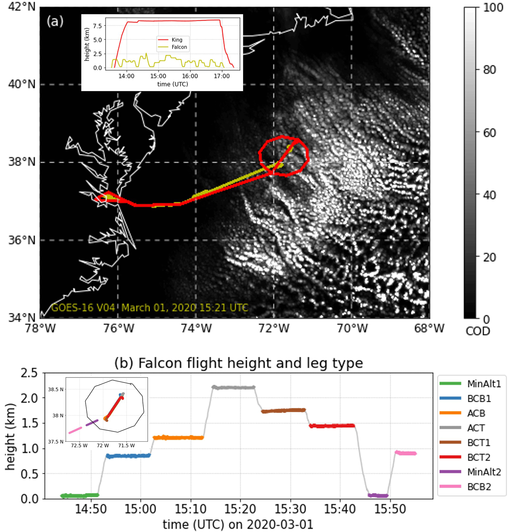
Figure 1(a) ACTIVATE flight tracks for Falcon (yellow) and King Air (red) aircraft on 1 March 2020 (RF13) overlaid with the GOES-16 satellite-measured cloud optical depth (COD) at 15:21 UTC. The insert shows the time series of the flight altitude for both aircraft. (b) Time and height of the eight Falcon flight legs within or near the dropsonde array domain. The insert is the horizontal location of the eight flight legs and the dropsonde domain (thin black line). Acronyms of flight leg types: BCB is for below cloud base, ACB is for above cloud base, ACT is for above cloud top, BCT is for below cloud top, and MinAlt is for minimum altitude (∼ 150 , above ground level).
2.2 Forcing and evaluation data
Table 1 lists the aircraft measurements used in this study. These observational data are used mainly for two purposes: driving models as initial and boundary conditions and evaluating model results. Satellite measurements and reanalysis data are also used to supplement the aircraft measurements to give a more complete view and fill data gaps when aircraft data are unavailable. Specifically, the liquid water path (LWP) and the ice water path (IWP) are retrieved from the GOES-16 geostationary satellite using the Visible Infrared Solar-Infrared Split-Window Technique (VISST) (Minnis et al., 2008, 2011) algorithm from the NASA Langley Satellite Cloud Observations and Radiative Property retrieval System (SatCORPS). ERA5 reanalysis data (Hersbach et al., 2020) are used to provide model initial and boundary conditions to drive the WRF–CRM simulation and to supplement the large-scale forcing used by WRF–LES and E3SM SCM. More details on the large-scale forcing are given in the Sect. 2.3.
Table 1Aircraft measurements used in this study.
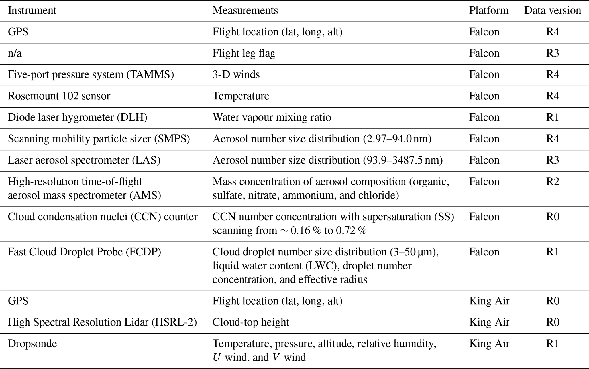
n/a: not applicable.
2.3 Model simulations
The SCM used in this study is based on the Energy Exascale Earth System Model (E3SM) version 2 (Golaz et al., 2022; Bogenschutz et al., 2020). It includes a deep convective parameterization from Zhang and Mcfarlane (1995) with the modification in convective trigger from Xie et al. (2019) to improve the diurnal cycle of precipitation, a two-moment microphysics scheme from Gettelman and Morrison (2015) (MG2), and a Cloud Layers Unified By Binormals (CLUBB) (Golaz et al., 2002; Larson and Golaz, 2005) parameterization for turbulence, shallow convection, and macrophysics all together. Some parameters of these schemes were systematically re-tuned to improve the overall performance of subtropical stratocumulus clouds (Ma et al., 2022). Aerosols generally require a long spin-up time that is unrealistic during the relatively short SCM case durations. Instead of directly using the aerosol scheme, three options have been implemented in E3SM SCM to treat aerosols: specifying droplet and ice number concentrations to “bypass” ACIs, using “prescribed” aerosols from a 10-year E3SM climatology simulation under present-day forcing conditions, or using “observed” aerosol information if available (Bogenschutz et al., 2020). The information of three lognormal distribution modes of aerosols (Aitken, accumulation, and coarse) is needed in the prescribed and observed methods to replace the output from the aerosol scheme, which is a three-mode Modal Aerosol Module (MAM3) (Liu et al., 2012) in the E3SM SCM configuration. Note that this differs from the default MAM4 scheme (Liu et al., 2016) in the E3SM GCM. The observed method currently does not include vertical variation in the aerosols (i.e. observed aerosol information is applied to all vertical layers from the surface to the model top). Therefore, to investigate ACIs and the impact of aerosol vertical distribution on clouds, we use a prescribed–observed hybrid method in this study in which we replace the prescribed aerosol input data with aircraft-measured aerosols or idealized conditions. Note that in this configuration we can only study the impact of aerosols on clouds but not the interactive microphysical and dynamical feedback to aerosols because when aerosols are prescribed, model representations of aerosol sink and source processes such as emissions, scavenging, and deposition are disabled.
E3SM SCM is driven by prescribed large-scale forcing data (i.e. advective tendencies and vertical velocity) and surface turbulent fluxes with a nudging timescale of 3 h to reduce biases in the atmospheric mean state. We use the same forcing data as Li et al. (2022) in their WRF–LES simulations over the dropsonde region (red circle in Fig. 1a). The large-scale forcing fields are shown in Fig. 2. The environment exhibits strong subsidence with cold and dry advection in the lower atmosphere. The near-surface cold and dry air and relatively high SST (not shown) lead to large surface latent (∼ 400 W m−2) and sensible (> 200 W m−2) heat fluxes. Although these data are obtained from the ERA5 reanalysis, which exhibits a cold and dry bias in MBL (Seethala et al., 2021), the wind structure is well captured (Chen et al., 2022), and the ERA5 divergence agrees well with that derived from the ACTIVATE dropsonde array (Li et al., 2022). Overall, it has been shown that the ERA5-derived large-scale forcing and surface turbulent fluxes can reasonably reproduce clouds and boundary layer for this case in WRF–LES simulations (Li et al., 2022, 2023).
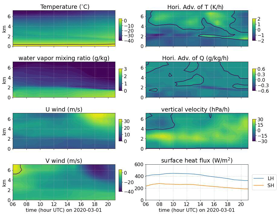
Figure 2Large-scale environmental conditions, large-scale forcing (horizontal advection and vertical velocity), and surface forcings (latent and sensible heat fluxes) over the dropsonde region from ERA5 reanalysis. The black lines in the contour panels mark the zero contour.
The WRF–CRM (Chen et al., 2022) and WRF–LES (Li et al., 2022, 2023) simulations are also used for intercomparison with the E3SM SCM. The WRF–CRM has an outer domain at a 3 km horizontal grid and an inner domain at a 1 km convective-resolving resolution with an interactive land option and prescribed SST from ERA5. It is able to reproduce the “cloud street” feature seen in satellite images (Chen et al., 2022). The comparison of the WRF–CRM nested simulation with ERA5 reanalysis over the dropsonde region and the results of SCM and LES driven by WRF–CRM forcings are given in Figs. S1–S4 in the Supplement. The WRF–LES simulation has a domain size of 60 km × 60 km with a 300 m horizontal grid spacing (Li et al., 2022). Its large-scale forcing and surface turbulent fluxes are prescribed from ERA5, as described above. Nudging is applied only to horizontal winds at a timescale of 1 h, with temperature and moisture freely evolving. In both CRM and LES simulations, a uniform cloud droplet number concentration (Nd) was specified so that ACI processes were bypassed. The specified Nd value of 450 cm−3 was obtained from a previous version of the Fast Cloud Droplet Probe (FCDP) measurements (Li et al., 2022). The newer version of FCDP (see Table 1) with an updated instrument calibration gives a smaller Nd value. As will be seen later (e.g. Fig. 5), the E3SM SCM simulation is more consistent with the updated FCDP data. Note that we keep the original setups of prescribed Nd in CRM and LES for consistency with previous studies (Chen et al., 2022; Li et al., 2022, 2023). As all the simulations are available for the same case, we have the opportunity to demonstrate the value of combining CRM and LES with SCM for the process level understanding of ACIs.
All the E3SM SCM, WRF–LES, and WRF–CRM simulations are initiated at 06:00 UTC on 1 March 2020. With a quick initial spin-up, marine CAO clouds develop between 1 and 2 (above ground level) and then display a gradual reduction in vertical extent, cloud-top height, and cloud water content (Figs. 3 and 4). These are generally consistent with ERA5 reanalysis. Note that the ERA5 cloud properties are also obtained from the reanalysis host model. Both E3SM SCM and WRF–LES generate 100 % cloud fraction most of the time, while the WRF–CRM simulated cloud fraction decreases with time. This is associated with the success of capturing the cloud roll structure in WRF–CRM (Chen et al., 2022). However, this roll structure fails to be simulated in WRF–LES and is not parameterized in E3SM SCM. Both liquid and ice hydrometeors are produced and transformed into rain and snow particles. The total ice (including snow) water content is about 1 order of magnitude smaller than total liquid water (including rain) (Fig. 3b and c). In our further analyses, we ignore ice and only focus on liquid clouds for simplicity. All simulations produce a weak mean surface precipitation of less than 2 mm d−1 (Fig. 4b). The evaluation of surface precipitation versus observations is not conducted here due to the lack of surface measurements and the limited ability of satellite measurements to detect weak precipitation from low-level MBL clouds (e.g. Battaglia et al., 2020).
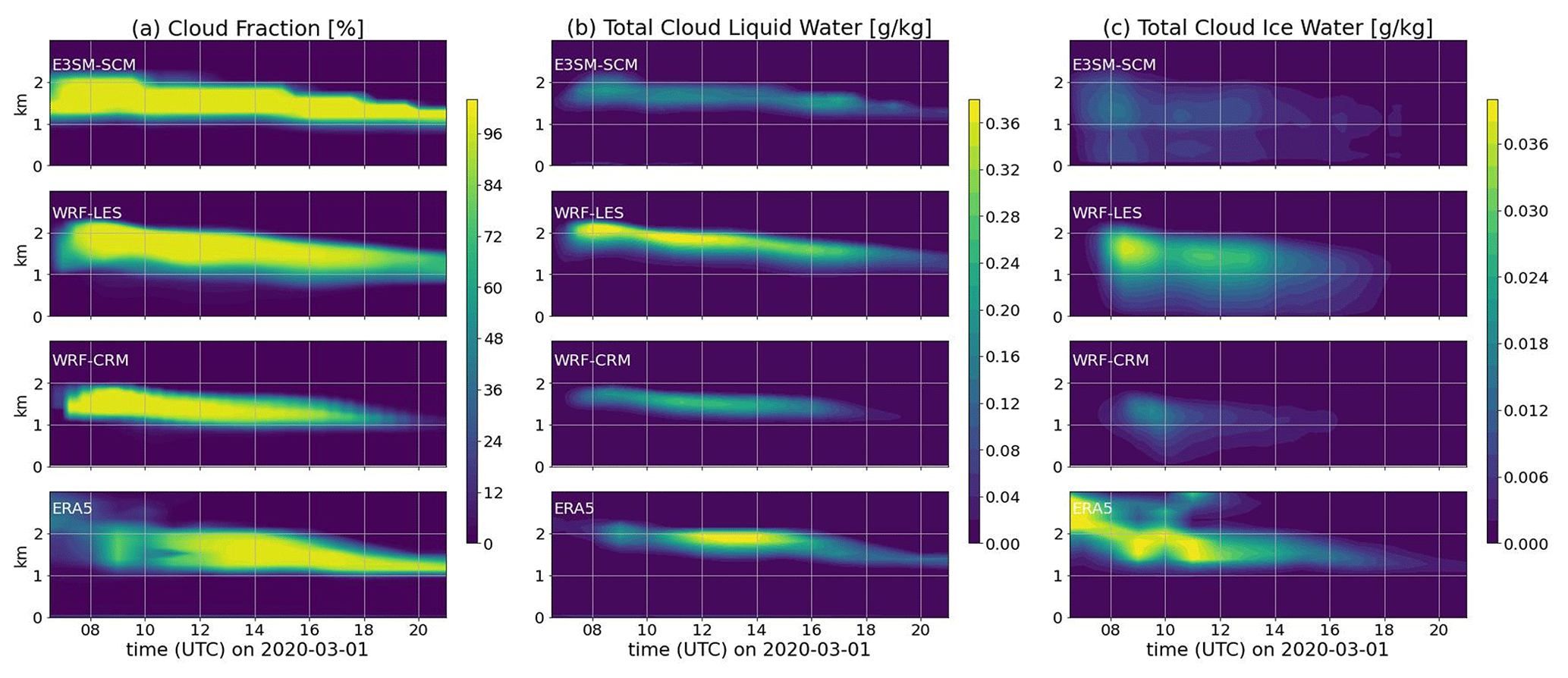
Figure 3Time–height cross sections of cloud fraction, total liquid water, and total ice water produced from different model simulations.
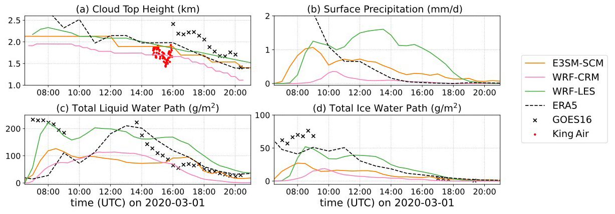
Figure 4Time series of model simulations (lines) compared with observation (dots) for the 1 March 2020 case. Observational data are from King Air HSRL-2 for cloud-top height, GOES-16 retrievals for cloud-top height, total liquid (including rain), and total ice (including snow) water paths for which the data points at a solar zenith angle greater than 65° are removed.
Figure 4a shows the time series of cloud-top height compared with GOES-16 satellite measurements and HSRL-2 measurements from the King Air aircraft. It should be noted that although both are measured from above the cloud, the satellite-measured cloud-top height is about 1 km higher than the aircraft lidar measurement. This might be due to some very thin cirrus clouds that skewed the satellite-measured brightness temperature lower. As this is only a case study, we do not attempt to address whether the satellite measurement has any systematic bias. HSRL-2 detects the top of each individual cloud, which is usually lower than or, at best, equal to the highest cloud top within the area. Therefore, we only compare model results with the highest values of the HSRL-2 measurements. The cloud-top heights in models are derived by integrating cloud-fraction-weighted height levels downward, as described in Varble et al. (2023). E3SM SCM and WRF–LES produce similar cloud-top heights (Fig. 4a), consistent with the highest observed cloud tops in HSRL-2. Ignoring the model spin-up period and high solar zenith angle when satellite retrievals encounter large biases, E3SM SCM and WRF–CRM also reproduced the total liquid water path, while WRF–LES overestimates it by ∼ 50 % after 14:00 UTC compared to the satellite retrievals (Fig. 4c). For the total ice water (including snow), with only a few valid data points in GOES-16 retrievals around 17:00 UTC, SCM and LES seem to overestimate it although the overall magnitude is small (Fig. 4d).
Figure 5 shows the vertical profiles of atmospheric state and cloud variables compared to dropsondes, ERA5 forcing data, and in situ aircraft measurements. The atmospheric state variables are constrained by ERA5 reanalysis, which has a colder and drier boundary layer than the dropsonde measurements (Fig. 5a and b; also reported in Seethala et al., 2021). However, the Falcon data in the boundary layer are also colder and drier than the dropsonde measurements. These differences reflect observational uncertainties to some extent. All models are generally consistent with the observations. However, they do show different temperature biases. E3SM SCM tends to be warmer while WRF–LES and WRF–CRM tend to be colder than the dropsondes. This bias is seen throughout the entire simulation period (not shown), indicating different performances of model parameterizations in E3SM SCM and WRF–LES as they used the same initial conditions and large-scale forcing.
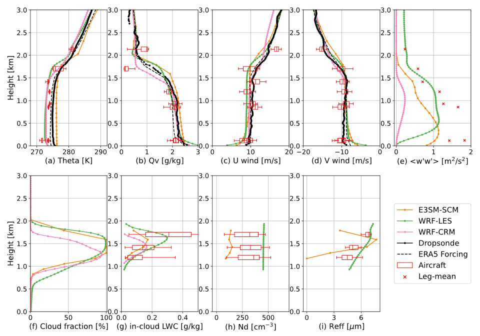
Figure 5Vertical profiles of atmospheric state, vertical velocity variance, and cloud variables over the analysis domain compared with dropsonde and Falcon measurements. Model profiles are averaged between 15:00 and 16:00 UTC during the aircraft measurements. The box plots indicate the interquartile ranges of the aircraft measurements in each flight leg, and the whiskers indicate 5th and 95th percentiles, while the red crosses represent vertical velocity variances calculated from 1 Hz measurements in each flight leg. For cloud microphysical variables, a threshold of in-cloud liquid water content of 0.02 g m−3 and cloud droplet number of 20 cm−3 is applied for both model results and aircraft measurements.
WRF–LES and WRF–CRM both use prescribed Nd obtained from a previous version of Falcon aircraft measurements during the ACB flight leg, which is higher than the re-calibrated value in the current version (Fig. 5h). They produce similar in-cloud liquid water content (LWC) below 1.5 km, but WRF–CRM produces lower LWC above 1.5 km because of its lower cloud-top height (Fig. 5g). WRF–LES produces a slightly greater droplet effective radius (Reff) than the aircraft measurements (Fig. 5i). Together with the large Nd, both contribute to large cloud LWC and LWP. WRF–CRM uses bulk microphysics and does not have Reff. The E3SM-SCM-simulated LWC is consistent with aircraft measurements during the BCT2 flight leg near 1.4 but lower than the other two in-cloud flight legs (Fig. 5g). It also produces larger sizes of cloud droplets around 1.5 (Fig. 5i) but produces much lower Nd (Fig. 5h). Possible causes of the underestimation of Nd include an underestimation of both the aerosol number concentration (see Sect. 4.1) and turbulence (Fig. 5e). Weaker vertical velocity variance than observations is a general bias seen in E3SM for the entire ACTIVATE campaign (Brunke et al., 2022) which may cause lower supersaturation (SS) which activates fewer cloud condensation nuclei (CCN) into cloud droplets (e.g. Kirschler et al., 2022). We further investigate these two factors in Sect. 4.1.
The previous section suggests that the underestimation of Nd in E3SM may be partly due to the underestimation of the aerosol number concentration in the climatological aerosol input for this CAO case. In this section, we use observed aerosols to drive E3SM SCM and conduct two sets of sensitivity studies on aerosol number size distribution and composition to investigate how the input aerosol properties impact clouds and radiative forcing.
4.1 Sensitivity to different aerosol number size distributions
We first test the sensitivity of SCM simulations to different aerosol number size distributions using the measurements from five out-of-cloud legs within or near the dropsonde domain (Fig. 1b). The Falcon aircraft during the ACTIVATE campaign was equipped with a scanning mobility particle sizer (SMPS) and a laser aerosol spectrometer (LAS) (Table 1) to measure the aerosol number size distribution from 2.97 to 94.0 nm (for SMPS) and 93.9 to 3487.5 nm (for LAS), respectively. We merge the two instruments and fit them into three lognormal modes, namely Aitken, accumulation, and coarse modes. For the three parameters in the lognormal distribution function, namely mode total number concentration (N), mode geometric median diameter (μ), and standard deviation (σg), we only fit N and μ. Because σg is also prescribed in other parts of the model (e.g. radiation calculation), we fix σg with the E3SM-prescribed values (1.6 for Aitken and 1.8 for accumulation and coarse modes) for consistency. A sensitivity test shows that using freely fitted N, μ, and σg in E3SM SCM only yields a minor difference compared to using fixed σg (not shown). For most flight legs, the fitting of coarse-mode aerosols exhibits large uncertainties due to limited samples with large variation. As the coarse-mode aerosol number concentration is usually orders of magnitude smaller than that of the Aitken and accumulation modes, the poor fitting of coarse-mode aerosols is not expected to impact the cloud microphysical properties much.
The centre panel of Fig. 6 shows the fitted aerosol number size distributions from different flight legs overlapped with E3SM climatological aerosols near the cloud base height (∼ 900 ). The individual fitting of the three modes, as well as the fitting parameters in each flight leg, is shown in the surrounding panels. It is clearly seen that the below-cloud flight legs (MinAlt and BCB) generally have more aerosols, especially in the accumulation mode, than the above-cloud-top flight leg (ACT). The E3SM climatological aerosols at the cloud base show more and larger Aitken-mode particles and fewer coarse-mode particles than all flight leg measurements. For accumulation-mode particles that are most important for CCN number concentration, the E3SM climatology lies between the ACT leg and below-cloud legs. Although the ACT leg does not represent cloud base aerosol conditions that are more relevant to the aerosol activation process, the inclusion of this leg provides information on how SCM performs in a clean environment.
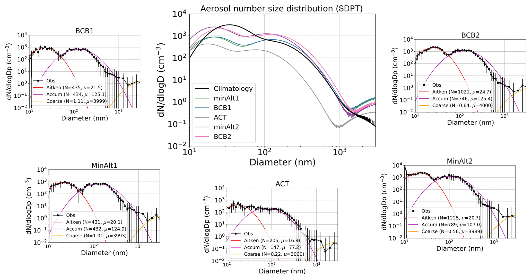
Figure 6The plot in the centre shows the aerosol number size distribution from (black) the E3SM-prescribed aerosol file from a climatological run near the height of simulated cloud base (∼ 900 ) and (colours) the aircraft measurements averaged for each out-of-cloud flight leg fitted to three-mode lognormal distributions. The surrounding plots show the mean observed aerosol number size distribution and 1 standard deviation (vertical lines) from each out-of-cloud flight leg and the lognormal fittings for the Aitken, accumulation, and coarse modes. The fitting parameters (N in cm−3 and μ in µm) are shown in the figure legends with the geometric standard deviation (σg) set as 1.6 for Aitken mode and 1.8 for the accumulation and coarse modes. All data are converted for standard pressure (1013.25 hPa) and temperature (273.15 K) conditions.
The fitted lognormal parameters from aircraft measurements are used to calculate and replace the variables in the E3SM-prescribed aerosol input data. The averaged chemical component fractions below 1.5 km from E3SM aerosol climatology are used to partition the measured aerosol number size distribution so they all have the same fraction of aerosol components. The sensitivity to different aerosol chemical compositions will be discussed in Sect. 4.2, while in this section, we only focus on how aerosol number concentration impacts clouds in E3SM SCM. The prescribed aerosol number concentration has no information on the variation with height. This height-independent assumption is usually used in SCM configurations with observed aerosols (e.g. Liu et al., 2007, 2011; Klein et al., 2009), assuming that only cloud base aerosols are involved in the cloud droplet nucleation process (e.g. Liu et al., 2011).
All simulations are run from 06:00 to 21:00 UTC, which is the same as the previous simulations in Sect. 3. To compare with aircraft measurements, we average the simulations between 15:00 and 16:00 UTC (aircraft sampling time) and plot the vertical profiles in Fig. 7. The large variation in the CCN number concentrations has a very small impact on the cloud fraction and in-cloud LWC. Instead, it mainly impacts the cloud droplet number and size, so more CCN leads to more cloud droplets and a smaller droplet size. However, all the simulations underestimate Nd compared to the aircraft measurements. Another sensitivity test shows that the underestimation of both the aerosol number concentration and turbulence strength contributes to the underestimation of Nd in this case. When doubling the vertical velocity variance to be consistent with the observations and using observed aerosols below the cloud base in the SCM, the simulated Nd then becomes more similar to the aircraft measurements (Fig. 8).
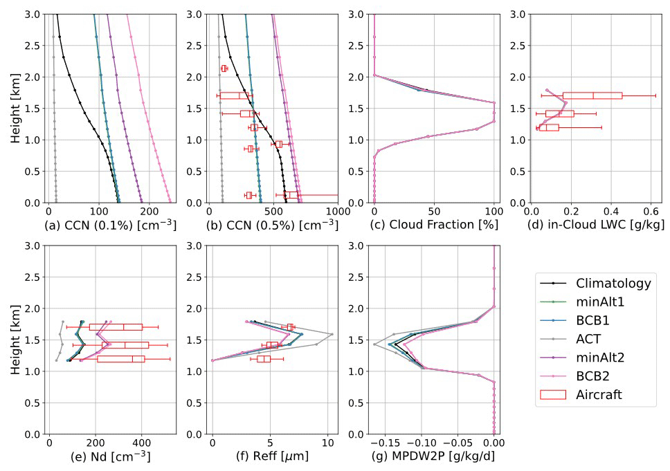
Figure 7Vertical distributions of (a) CCN number concentrations at 0.1 % and (b) 0.5 % supersaturation, (c) cloud fraction, (d) in-cloud LWC, (e) Nd, (f) Reff, and (g) cloud water tendency from the conversion-to-precipitation processes (MicroPhysics tendency Due to Water to Precipitation, MPDW2P) in E3SM SCM simulations with different aerosol specifications averaged between 15:00 and 16:00 UTC. Aircraft measurements of cloud microphysical properties overlaid are the same as in Fig. 5.
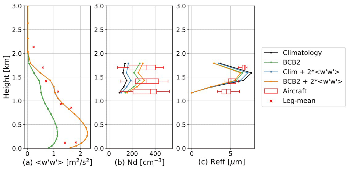
Figure 8(a) Vertical velocity variance , (b) cloud droplet number concentration Nd, and (c) cloud droplet effective radius Reff averaged between 15:00 and 16:00 UTC, which is when the aircraft measurements (shown with red crosses and boxes) were made. In the figure legend, “Climatology” is the original SCM run with prescribed aerosol concentration, “BCB2” is the SCM run with aerosol number concentration from the aircraft measurement at BCB2 leg, and “2* ” means that the vertical velocity variance is enhanced by the factor of 2 in the SCM aerosol activation scheme.
We further plot the simulated cloud droplet number size distribution at three different heights in Fig. 9 with simulations using prescribed aerosols from different flight legs. Compared with the aircraft-measured cloud droplet size distribution at each height, the gamma distribution assumption of the cloud droplet spectrum in MG2 generally captures the observed droplet size distribution and reproduces the mean droplet size well but fails to reproduce the observed peak of Nd at all three heights. A similar sharp peak of Nd around 10 to 20 µm was also observed by aircraft over the Southern Ocean, and the model with the same MG2 microphysics scheme underestimated Nd in a similar way (Gettelman et al., 2020).
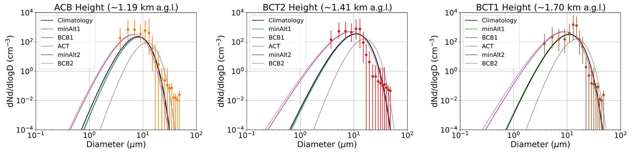
Figure 9E3SM-SCM-simulated cloud droplet size distribution at the height of three in-cloud flight legs (ACB: ∼ 1.20 km, BCT2: ∼ 1.44 km, and BCT1: ∼ 1.74 km). Note that the flight leg name and height in the title above each panel specify from where the cloud data are taken to make the plot, while the flight leg names in each panel legend describe from where the aerosol data are taken to drive the corresponding E3SM SCM simulations. The dots and error bars represent aircraft measurements at the corresponding flight legs and the 5th and 95th percentiles.
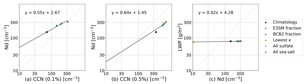
The strong impact of the aerosol number size distribution on cloud microphysical properties (number and size) in SCM indicates that E3SM shows a strong Twomey effect (Twomey, 1977, 1959) for this case. The change in Nd is tightly related to the change in the CCN number concentration (Fig. 10a and b). A recent study of long-term E3SM simulation over the eastern North Atlantic suggests that the Nd susceptibility (i.e. relationship) in E3SM may be too strong comparing to observations (Tang et al., 2023). Previous studies showed that Nd is also impacted by other factors such as updraft velocity (e.g. Kirschler et al., 2022; Chen et al., 2016), which indicates a potential need to examine updraft velocity in E3SM in the future. The surface downward shortwave flux is largely impacted by the change in the cloud droplet number and size due to different aerosol specifications (Fig. 11c), with the differences reaching up to 100 W m−2 during the analysis period (15:00–16:00 UTC).
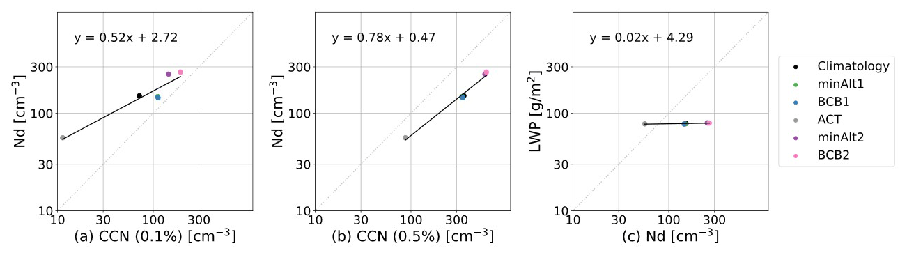
Figure 10Scatter plot between simulated Nd and CCN at two different supersaturations and between LWP and Nd. The linear fit equations representing and are noted in each panel. The standard errors in the slope and intercept for each panel are (0.082, 0.37), (0.048, 0.28), and (0.007, 0.037), respectively.
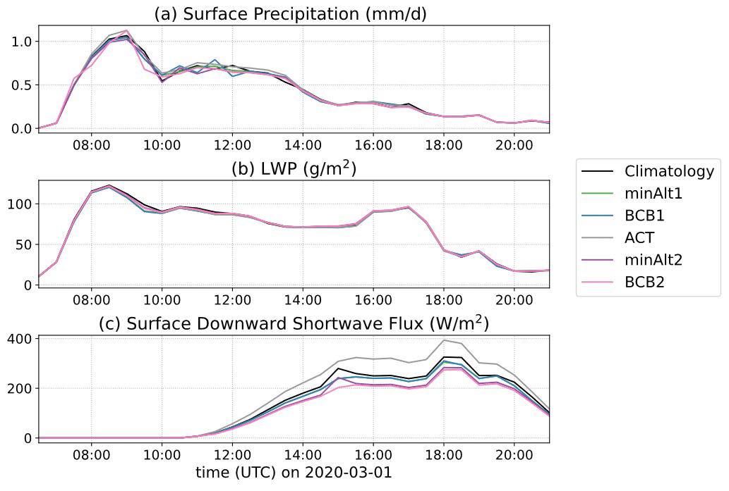
Figure 11Time series of (a) surface precipitation, (b) LWP, and (c) surface downward shortwave flux from E3SM SCM simulations with different aerosol specifications.
In contrast to the strong Twomey effect, the weak impact of aerosols on cloud macrophysical properties (cloud fraction and cloud water content; see Fig. 7) indicates a very weak LWP adjustment in E3SM. The LWP susceptibility is almost zero (Fig. 10c). The slightly positive slope is likely due to the suppression of precipitation processes (Fig. 7g) when cloud droplet sizes decrease in response to more aerosol particles and cloud droplets. However, the magnitude of the precipitation rate change is so small that it can barely change the overall LWP and surface precipitation (Fig. 11). In the CAO case, LWP and other cloud macrophysical properties are likely determined by the strong dynamical and thermodynamical controls (e.g. strong cold-air advection, surface turbulent heat fluxes, and subsidence in Fig. 2). The change in aerosols mainly impacts cloud microphysical properties through altering the cloud droplet number and size, which is shown to have a minimal effect on cloud LWP for this case. We believe that under the synoptic conditions with weaker large-scale forcing and/or stronger precipitation, aerosol effects on cloud macrophysical properties may be stronger. This weakly linear relation in the E3SM SCM simulations is different from the non-linear relation seen in the long-term E3SM GCM run (Tang et al., 2023).
4.2 Sensitivity to different aerosol composition
Aerosol chemical composition is an important property that determines aerosol hygroscopicity (κ) and further impacts the likelihood of aerosols serving as CCN and activating into cloud droplets. In E3SM, the overall κ is calculated assuming internal mixing of aerosol species within each mode and external mixing among different modes (Liu et al., 2012; Liu et al., 2016). Although the aerosol chemical composition also impacts the overall size distribution in reality (Shrivastava et al., 2017), this mechanism is not implemented in the current E3SM. In this section, we investigate the differences in the aerosol composition used in E3SM and observed by Falcon aircraft measurements. We further test the sensitivity of simulated clouds to aerosol composition, and ultimately hygroscopicity, using simulated and observed values and assuming a few extreme conditions.
Figure 12a shows the aerosol mass concentrations for each component in the E3SM aerosol climatology. Most of the aerosols are concentrated within the boundary layer below 1 km, with the Aitken and accumulation modes dominated by sulfate, and the coarse mode dominated by sea salt aerosols. Figure 12b–f all use the same observed aerosol number size distribution, fitted from the BCB2 flight leg but combined with different aerosol component fractions. The setting of “E3SM fraction” uses the aerosol composition from E3SM-prescribed aerosols at the level closest to the BCB2 leg (near ∼ 900 ). The “BCB2 fraction” uses the aerosol composition from the aerosol mass spectrometer (AMS) measurements at the BCB2 leg. Among the five components in AMS measurements (Table 2), sulfate (SO4) and organics are the two dominant species observed during ACTIVATE (Dadashazar et al., 2022a). They are also the only two species specified in E3SM, with assumptions of the composition of organics. Here we assume all AMS-measured organics are secondary organic aerosols (SOAs) and then calculate new aerosol concentrations using the observed mass fraction of SO4 and SOAs while keeping the fraction of other species the same in E3SM. It can be seen that the aircraft-measured SO4 : SOA ratio is about 1:1 in mass and much smaller than in the E3SM climatology. This change results in a reduction in the κ value from 0.46 to 0.31 (Table 2) as the hygroscopicity of SOAs is much smaller than SO4.
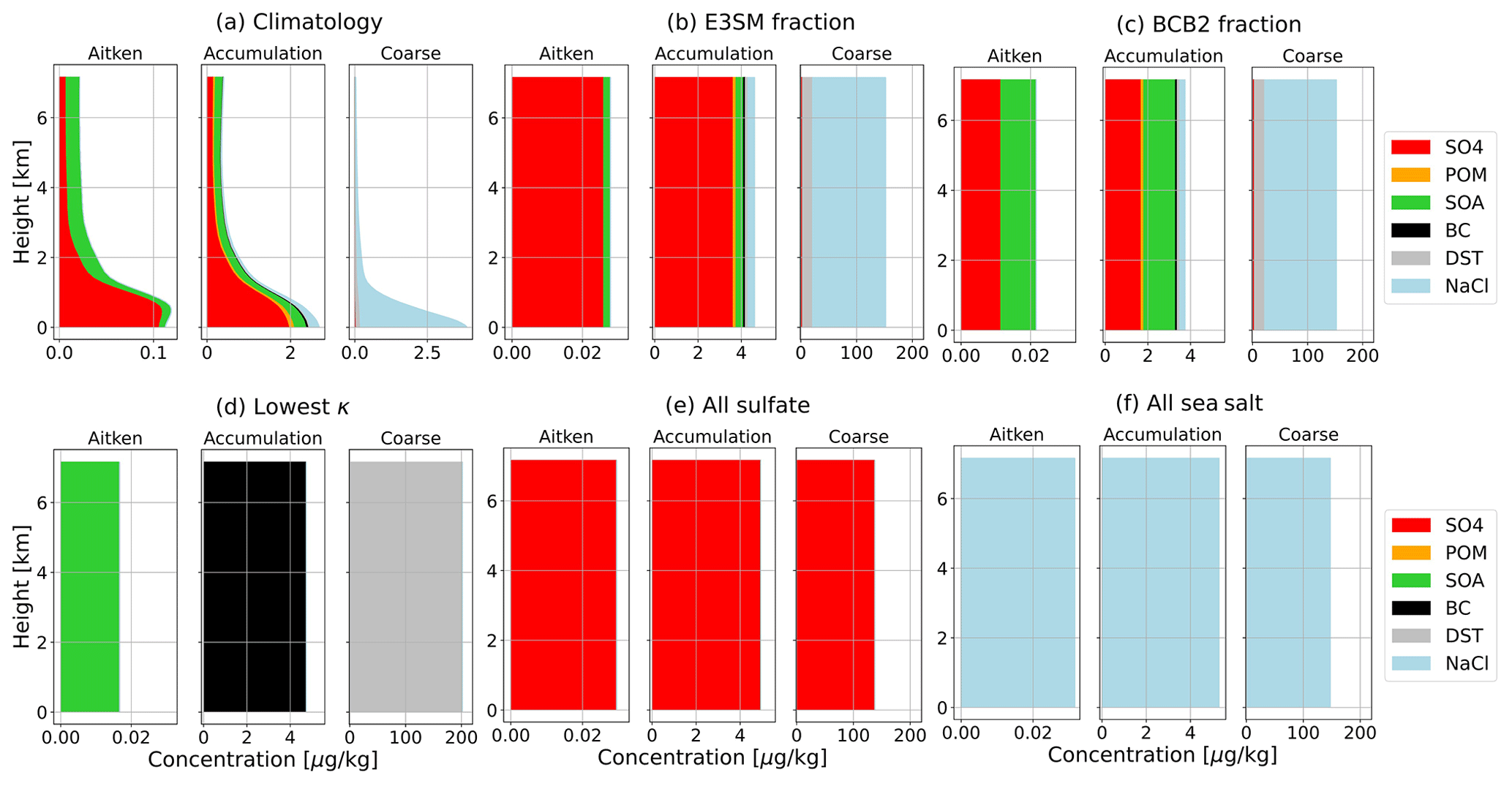
Figure 12Different settings of the aerosol mass concentration for each component used in E3SM from (a) climatology from the E3SM GCM output; (b) applying the composition fraction from E3SM climatology aerosols at the height of the BCB2 flight leg; (c) using an observed fraction of sulfate and organics (assuming SOAs) from the BCB2 flight leg; and (d–f) assuming all aerosols are the lowest-hygroscopicity species (“lowest κ” ) in that mode, in sulfate, and in sea salt aerosols, respectively. Note the different x axis in panels (a) and (b)–(f). In panels (b)–(f), the aerosol number size distributions are from aircraft measurements in the BCB2 flight leg and assume no vertical variation. Notation of aerosol species is as follows: SO4 is for sulfate, POM is for primary organic matter, SOAs is for secondary organic aerosols, BC is for black carbon, DST is for dust, and NaCl is for sea salt.
Table 2Fraction of aerosol species in each mode (Aitken, accumulation, and coarse modes) specified in five sensitivity tests. The dash (“–”) means that the species is not accounted for in the mode.
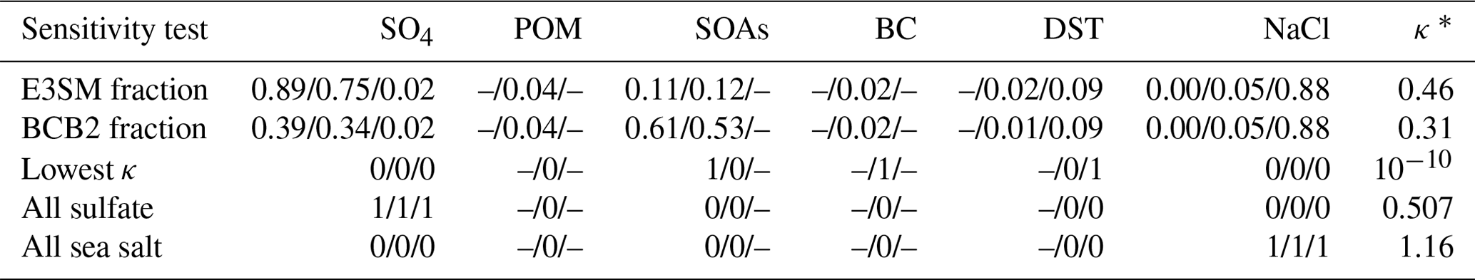
∗ κ is calculated from the accumulation mode.
Three other idealized aerosol settings in extreme conditions are provided for the sensitivity test. The first one, lowest κ, is the option to use the lowest-hygroscopicity species in each mode. The second option assumes all aerosols are SO4 aerosols, and the third one assumes all sea salt aerosols. The corresponding aerosol fraction in each mode and the overall κ values are given in Table 2. The lowest-κ option has an extremely low κ value of 10−10 in the accumulation mode, while the “all sea salt” option has a large κ of 1.16. The other options have κ values varying from 0.3 to 0.5.
The different aerosol hygroscopicity results in different CCN number concentrations (Fig. 13a and b). As SS increases, the critical diameter determining CCN number concentration decreases and becomes less sensitive to hygroscopicity. Therefore, except for the lowest κ sensitivity run in which the CCN number concentration is almost zero, the relative difference in the CCN number concentration with different aerosol composition settings is smaller for 0.5 % SS than 0.1 % SS. Nd and Reff are less sensitive to aerosol hygroscopicity ranging from 0.31 to 1.16 compared to CCN number concentration, and the cloud fraction and LWC vary even less. The only outlier is the lowest κ option with extremely low hygroscopicity. In this case, the extremely low CCN and Nd number concentration (but not zero as the E3SM model sets a lower limit of Nd = 10 cm−3 when a cloud exists) lead to an almost doubled droplet size (Fig. 13f). Therefore, it has much stronger surface downward shortwave radiation (Fig. 14c). The much larger droplet size also contributes to more precipitation conversion (Figs. 13g and 14a) and depletion of cloud liquid water (Fig. 14b). However, the impact is still very weak, and the estimated LWP susceptibility is 0.02 (Fig. 15c).
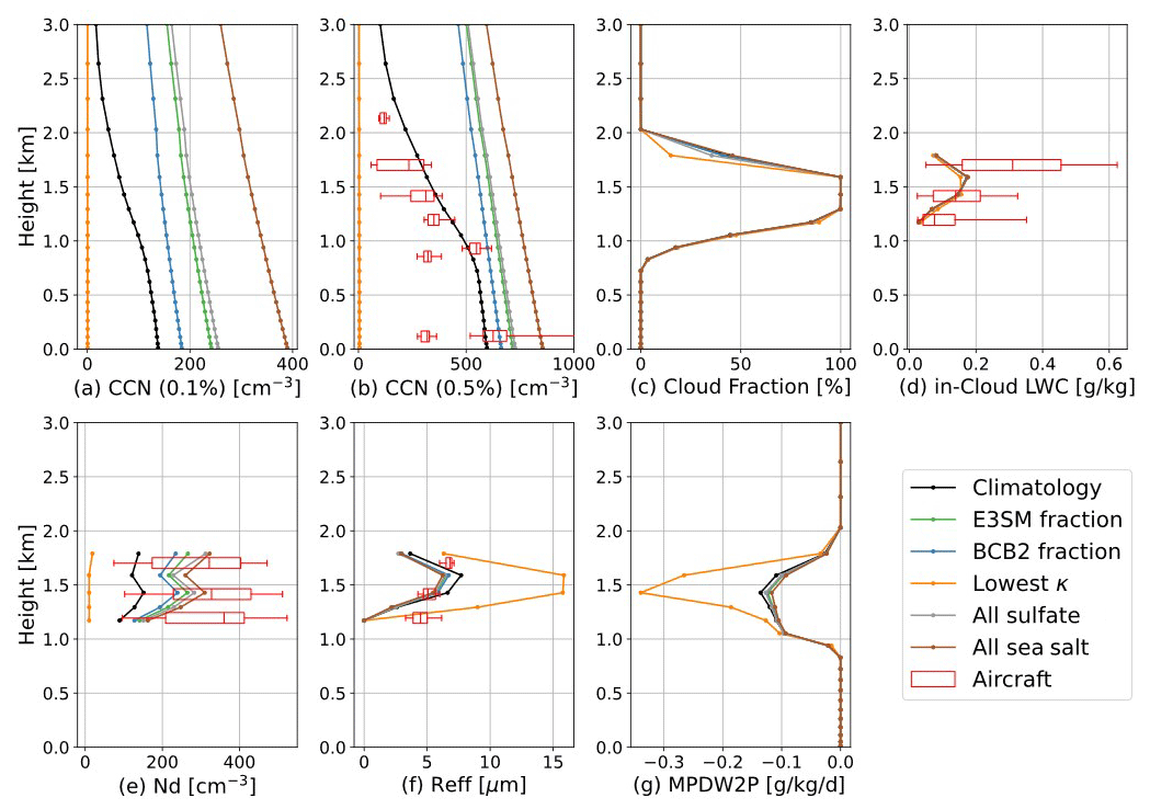
Figure 13Same as Fig. 7 but for E3SM SCM simulations with different aerosol composition profiles and the same aerosol number concentration (except for Climatology) from BCB2 measurements.
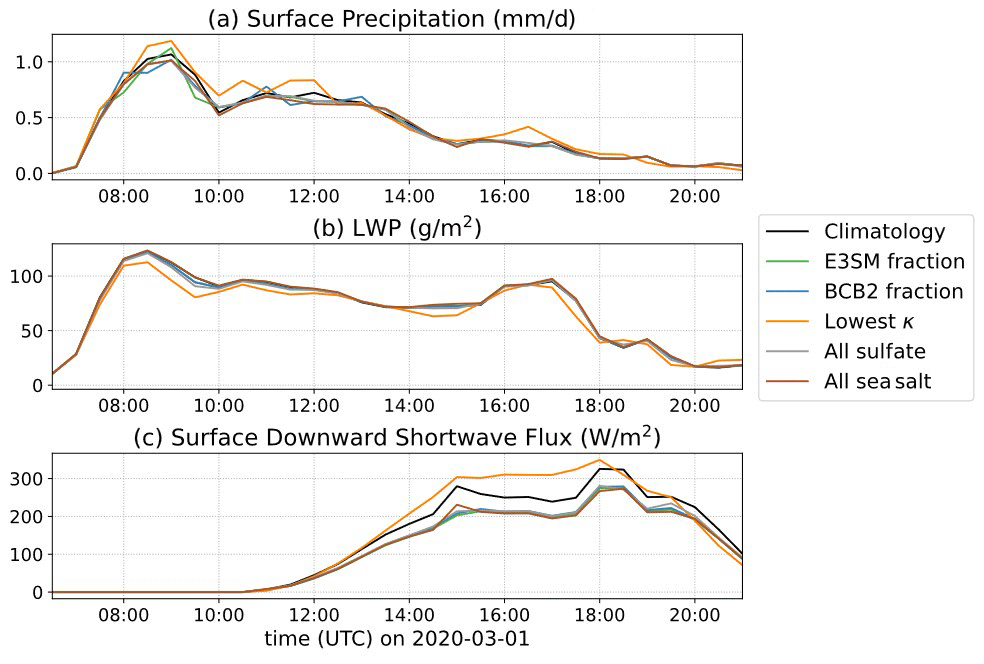
Figure 14Same as Fig. 11 but for E3SM SCM simulations with different aerosol composition profiles.
The previous section shows a weak linear relation in the E3SM SCM simulations associated with aerosol-induced precipitation suppression. This relation is different from the non-linear relations seen in observations and the long-term E3SM GCM simulations (Tang et al., 2023). In this section, we further investigate the LWP susceptibility and the related precipitation processes with additional SCM simulations.
Since some sensitivity tests conducted in Sect. 4 produce similar Nd values (Figs. 10c and 15c), we design new sensitivity tests with prescribed aerosols from aircraft measurements during the BCB2 leg and perturb the observed aerosol number concentration (Na) by 0.125, 0.25, 0.5, 2, 4, and 8 times for SCM to examine the susceptibility of LWP and surface precipitation due to Na perturbations. We also increase the value of a parameter in the E3SM parameterization, known as aggregation enhancement factor, by a factor of 10 to arbitrarily enhance the precipitation suppression effect. The time series of surface precipitation and LWP are shown in Fig. 16. With a higher Na, the surface precipitation is more suppressed, leading to more LWP remaining in the cloud. This effect is more obvious in the first few hours of the simulations. After ∼ 13:00 UTC, the differences in the surface precipitation and LWP induced by the perturbation of Na become much less distinguishable, which is consistent with the very weak relation seen at 15:00–16:00 UTC in Sect. 4. We hypothesize that the dynamical forcing and thermodynamical factors dominate the LWP budget and cloud evolution during this CAO event; therefore, the LWP adjustments due to aerosol perturbations become negligible. Further studies with more cases and associated statistical analyses are needed to verify this hypothesis.
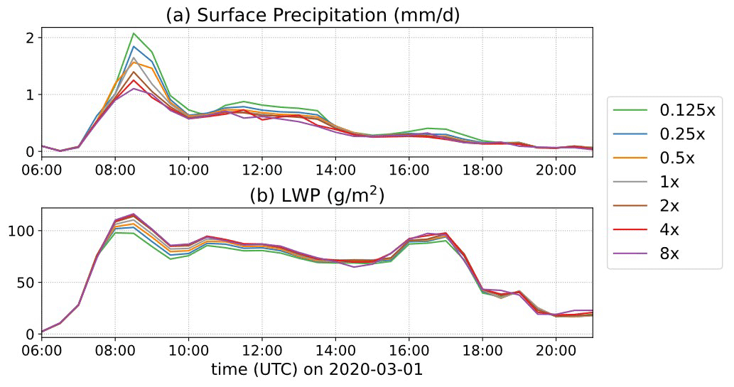
Figure 16Time series of (a) surface precipitation and (b) LWP from E3SM SCM simulations with different aerosol (Na) perturbations observed below cloud base during the CAO case.
The LWP susceptibility , which is now calculated by comparing the perturbed Na run and 1 × Na SCM simulations at each time step (1800 s) between 08:00 and 18:00 UTC, is shown in Fig. 17. Also shown is the susceptibility of surface precipitation . All the Na perturbation tests show a clear positive relation and a negative relation, demonstrating the precipitation suppression effect of aerosols in E3SM SCM. The spread in LWP and precipitation susceptibility becomes wider for higher Na perturbations, indicating that the precipitation suppression effect becomes more uncertain with increasing Na as cloud droplets become smaller and less likely to convert into precipitation. The mean of the median values is 0.03, close to the slopes estimated in Sect. 4. Again, this weak LWP susceptibility relation is likely due to the strong dynamical and thermodynamical control for this specific CAO case. Different cases may give different LWP susceptibility as other processes (e.g. entrainment) may dominate the effect (Mülmenstädt et al., 2024). Therefore, long-term SCM simulations with more cases are needed to obtain a statistically significant conclusion.
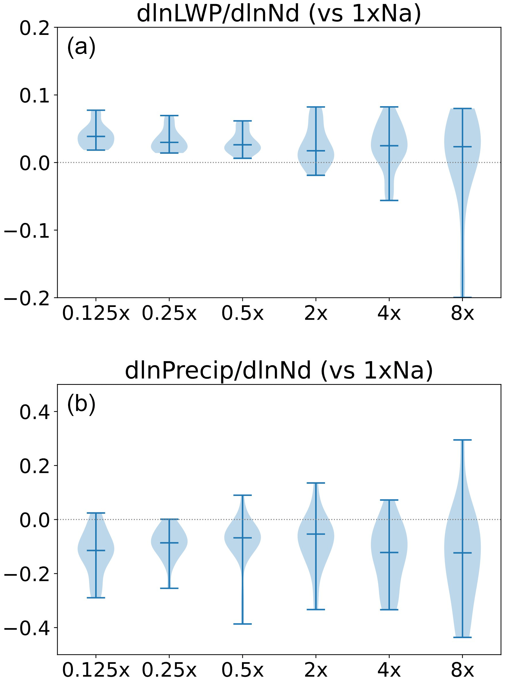
Figure 17Violin plots of (a) and (b) between 08:00 and 18:00 UTC for the different SCM simulations with perturbed Na in contrast to the default 1 × Na. The horizontal bars represent the upper bound, median value, and the lower bound of the data, while the shading represents the probability density of the data at the corresponding values.
Current Earth system models remain largely uncertain in simulating MBL clouds, and aerosol–cloud interactions related to MBL clouds have been underexplored over the WNAO. With the recent ACTIVATE field campaign conducted over the WNAO collecting in situ and remote-sensing measurements using two aircraft flying simultaneously at different heights, we conduct SCM simulations focusing on a selected CAO case, evaluate the results against field observations, and intercompare results with CRM/LES models. Furthermore, we perform several sets of SCM sensitivity experiments to understand the complex aerosol–cloud interactions related to MBL clouds over WNAO. This case study with a comprehensive set of aerosol sensitivity simulations provides insight into further designing long-term SCM simulations for statistical analysis, which is currently under consideration for a future study.
A unique feature of this study is the multi-scale model intercomparison using SCM, CRM, and LES models, which provides a comprehensive process level understanding of ACI in more detail compared to individual models. We conducted E3SMv2 simulations in the SCM mode and compared the results with two WRF model configurations at LES and CRM resolutions, respectively. Overall, the three models all capture the MBL cloud properties, while the E3SM SCM underestimates the cloud droplet number concentration and overestimates the droplet size. This is partly due to the relatively low number concentration of prescribed aerosols from the E3SM climatology compared to field observations in this case and partly due to underestimated updrafts that cannot activate enough aerosol particles into cloud droplets. Note that some parameters in E3SMv2 were tuned to improve the overall performance of subtropical stratocumulus clouds (Ma et al., 2022), but turbulence over the WNAO region is weakened compared to the pre-tuning version (close to E3SMv1) – even in a long-term GCM run (Brunke et al., 2022). The evaluation of SCM simulations against the ACTIVATE measurements can help improve turbulence representation over this region.
Several sets of sensitivity experiments are conducted to examine ACIs by changing the prescribed aerosol number size distribution and aerosol composition in E3SM SCM. Aircraft measurements at different heights are used to provide constraints of the aerosol perturbation. Changing aerosol number size distributions dramatically alters the CCN number concentration, thus largely impacting cloud droplet number concentration and size, further influencing the cloud radiative effect. However, the changing aerosol composition only shows dramatic impacts in the extremely low-hygroscopicity (κ) setting where only very few aerosols are activated into very large cloud droplets. Changing the overall κ from 0.31 to 1.16 has a smaller impact on cloud microphysical properties. The impact of aerosol composition on CCN concentration and cloud microphysics can be larger than that shown here as it may also change the aerosol size distribution (Shrivastava et al., 2017).
In contrast to the clear Twomey effect, the cloud fraction and water content are barely impacted by aerosol perturbations, with a very weak susceptibility of 0.02 during the time of aircraft measurements and 0.03 for the entire simulation period of this case. The slightly positive LWP adjustment is most likely due to the rain suppression effect (Albrecht, 1989). This contradicts the non-linear V-shaped curve shown in the long-term E3SM GCM run over the eastern North Atlantic Ocean (Tang et al., 2023; Varble et al., 2023). Whether this weak positive LWP susceptibility is a case-specific or cloud-regime-specific feature and whether SCM can reveal the same cloud susceptibility as the full GCM both require further study.
We also performed sensitivity tests to examine the impact of large-scale forcing data and aerosol vertical distribution on cloud simulations. Among the three models for intercomparison, E3SM SCM and WRF–LES are driven by the same large-scale and surface forcings derived from ERA5 reanalysis, while the WRF–CRM is run as a regional model with nested domains. With the same large-scale and surface forcings from the WRF–CRM, which has weaker subsidence and stronger low-level cold and dry air advection than the ERA5 forcings, the E3SM SCM and WRF–LES produce much thicker clouds than WRF–CRM (Figs. S2–S4). This indicates that a proper match of large-scale dynamics, sub-grid-scale parameterization, and model configurations is needed to obtain optimal model performance.
In the current SCM framework using observed aerosols, usually only one set of values for aerosol parameters (i.e. particle number size distribution and composition) is fed into the model regardless of the aerosol vertical distribution (Liu et al., 2011, 2007; Klein et al., 2009; Lebassi-Habtezion and Caldwell, 2015; Li et al., 2023). The prescribed aerosol information based on observations is usually taken from in situ measurements below the cloud base (e.g. Liu et al., 2011; Li et al., 2023), assuming that hygroscopic aerosol particles are readily activated into cloud droplets in the saturated air driven by updrafts. However, as aerosol concentration usually decreases with height in the lower atmosphere, regional aerosol vertical distribution may be changed by in-cloud scavenging, horizontal transport, and vertical mixing, which can further affect cloud microphysical properties by secondary activation above cloud base (Wang et al., 2013, 2020). We conducted a sensitivity experiment with a specified aerosol vertical distribution (Fig. S5), but the configuration of prescribed aerosols in the SCM only shows the response of clouds to aerosols given at the level of cloud formation. A more comprehensive consideration of complete aerosol processes (e.g. vertical transport, scavenging, and deposition) is needed (e.g. using WRF–CRM or E3SM) to include the cloud and dynamical feedback on aerosols and better understand the aerosol–cloud interactions.
The E3SMv2 model is available from the U.S. Department of Energy at https://doi.org/10.11578/E3SM/dc.20210927.1 (E3SM Project, 2021). The WRF community model is publicly available from the National Center for Atmospheric Research (NCAR) at http://www2.mmm.ucar.edu/wrf/users/ (NCAR, 2022), and the WRF–LES model code is specifically from https://code.arm.gov/lasso/lasso-wrf (LASSO Team, 2022).
The ACTIVATE aircraft data and GOES-16 satellite data are available from the NASA ACTIVATE project website at https://doi.org/10.5067/SUBORBITAL/ACTIVATE/DATA001 (ACTIVATE Science Team, 2020). ERA5 reanalysis data are available from the Copernicus Climate Change Service Climate Data Store (CDS) at https://doi.org/10.24381/cds.bd0915c6 (Hersbach et al., 2023a) and https://doi.org/10.24381/cds.adbb2d47 (Hersbach et al., 2023b).
The supplement related to this article is available online at: https://doi.org/10.5194/acp-24-10073-2024-supplement.
ST and HW designed the conceptional ideas. AS, HW, and XZ performed the mission planning and supervision. EC, KT, LZ, and CV participated in mission operation and data curation. ST conducted the SCM simulations, XYL conducted the WRF–LES simulations, and JC conducted the WRF–CRM simulations. ST performed the analysis and prepared the original draft. All co-authors contributed to the reviewing and editing of the paper.
At least one of the (co-)authors is a member of the editorial board of Atmospheric Chemistry and Physics. The peer-review process was guided by an independent editor, and the authors also have no other competing interests to declare.
Publisher's note: Copernicus Publications remains neutral with regard to jurisdictional claims made in the text, published maps, institutional affiliations, or any other geographical representation in this paper. While Copernicus Publications makes every effort to include appropriate place names, the final responsibility lies with the authors.
We thank two anonymous reviewers for constructive and insightful comments and suggestions. This work has been supported through the ACTIVATE Earth Venture Suborbital-3 (EVS-3) investigation, which is funded by NASA's Earth Science Division and managed through the Earth System Science Pathfinder Program office. The Pacific Northwest National Laboratory (PNNL) is operated for the U.S. Department of Energy by Battelle Memorial Institute under contract no. DE-AC05-76RLO1830. The simulations were performed using resources available through Research Computing at PNNL.
The PNNL authors have been funded by NASA under project no. 72170. The University of Arizona authors have been funded by NASA (grant no. 80NSSC19K0442). Christiane Voigt has been funded by the German Research Foundation (DFG) within the projects of SPP-1294 HALO (grant nos. VO1504/7-1 and VO1504/9-1).
This paper was edited by Matthew Lebsock and reviewed by two anonymous referees.
ACTIVATE Science Team: Aerosol Cloud meTeorology Interactions oVer the western ATlantic Experiment Data, ASDC (Atmospheric Science Data Center) [data set], https://doi.org/10.5067/SUBORBITAL/ACTIVATE/DATA001, 2020.
Albrecht, B. A.: Aerosols, Cloud Microphysics, and Fractional Cloudiness, Science, 245, 1227–1230, https://doi.org/10.1126/science.245.4923.1227, 1989.
Battaglia, A., Kollias, P., Dhillon, R., Roy, R., Tanelli, S., Lamer, K., Grecu, M., Lebsock, M., Watters, D., Mroz, K., Heymsfield, G., Li, L., and Furukawa, K.: Spaceborne Cloud and Precipitation Radars: Status, Challenges, and Ways Forward, Rev. Geophys., 58, e2019RG000686, https://doi.org/10.1029/2019RG000686, 2020.
Bock, L., Lauer, A., Schlund, M., Barreiro, M., Bellouin, N., Jones, C., Meehl, G. A., Predoi, V., Roberts, M. J., and Eyring, V.: Quantifying Progress Across Different CMIP Phases With the ESMValTool, J. Geophys. Res.-Atmos., 125, e2019JD032321, https://doi.org/10.1029/2019JD032321, 2020.
Bogenschutz, P. A., Tang, S., Caldwell, P. M., Xie, S., Lin, W., and Chen, Y.-S.: The E3SM version 1 single-column model, Geosci. Model Dev., 13, 4443–4458, https://doi.org/10.5194/gmd-13-4443-2020, 2020.
Bony, S. and Dufresne, J.-L.: Marine boundary layer clouds at the heart of tropical cloud feedback uncertainties in climate models, Geophys. Res. Lett., 32, L20806, https://doi.org/10.1029/2005GL023851, 2005.
Brunke, M. A., Ma, P.-L., Reeves Eyre, J. E. J., Rasch, P. J., Sorooshian, A., and Zeng, X.: Subtropical Marine Low Stratiform Cloud Deck Spatial Errors in the E3SMv1 Atmosphere Model, Geophys. Res. Lett., 46, 12598–12607, https://doi.org/10.1029/2019GL084747, 2019.
Brunke, M. A., Cutler, L., Urzua, R. D., Corral, A. F., Crosbie, E., Hair, J., Hostetler, C., Kirschler, S., Larson, V., Li, X.-Y., Ma, P.-L., Minke, A., Moore, R., Robinson, C. E., Scarino, A. J., Schlosser, J., Shook, M., Sorooshian, A., Lee Thornhill, K., Voigt, C., Wan, H., Wang, H., Winstead, E., Zeng, X., Zhang, S., and Ziemba, L. D.: Aircraft Observations of Turbulence in Cloudy and Cloud-Free Boundary Layers Over the Western North Atlantic Ocean From ACTIVATE and Implications for the Earth System Model Evaluation and Development, J. Geophys. Res.-Atmos., 127, e2022JD036480, https://doi.org/10.1029/2022JD036480, 2022.
Chen, J., Liu, Y., Zhang, M., and Peng, Y.: New understanding and quantification of the regime dependence of aerosol–cloud interaction for studying aerosol indirect effects, Geophys. Res. Lett., 43, 1780–1787, https://doi.org/10.1002/2016GL067683, 2016.
Chen, J., Wang, H., Li, X., Painemal, D., Sorooshian, A., Thornhill, K. L., Robinson, C., and Shingler, T.: Impact of Meteorological Factors on the Mesoscale Morphology of Cloud Streets during a Cold-Air Outbreak over the Western North Atlantic, J. Atmos. Sci., 79, 2863–2879, https://doi.org/10.1175/JAS-D-22-0034.1, 2022.
Corral, A. F., Braun, R. A., Cairns, B., Gorooh, V. A., Liu, H., Ma, L., Mardi, A. H., Painemal, D., Stamnes, S., van Diedenhoven, B., Wang, H., Yang, Y., Zhang, B., and Sorooshian, A.: An Overview of Atmospheric Features Over the Western North Atlantic Ocean and North American East Coast – Part 1: Analysis of Aerosols, Gases, and Wet Deposition Chemistry, J. Geophys. Res.-Atmos., 126, e2020JD032592, https://doi.org/10.1029/2020JD032592, 2021.
Dadashazar, H., Corral, A. F., Crosbie, E., Dmitrovic, S., Kirschler, S., McCauley, K., Moore, R., Robinson, C., Schlosser, J. S., Shook, M., Thornhill, K. L., Voigt, C., Winstead, E., Ziemba, L., and Sorooshian, A.: Organic enrichment in droplet residual particles relative to out of cloud over the northwestern Atlantic: analysis of airborne ACTIVATE data, Atmos. Chem. Phys., 22, 13897–13913, https://doi.org/10.5194/acp-22-13897-2022, 2022a.
Dadashazar, H., Crosbie, E., Choi, Y., Corral, A. F., DiGangi, J. P., Diskin, G. S., Dmitrovic, S., Kirschler, S., McCauley, K., Moore, R. H., Nowak, J. B., Robinson, C. E., Schlosser, J., Shook, M., Thornhill, K. L., Voigt, C., Winstead, E. L., Ziemba, L. D., and Sorooshian, A.: Analysis of MONARC and ACTIVATE Airborne Aerosol Data for Aerosol–Cloud Interaction Investigations: Efficacy of Stairstepping Flight Legs for Airborne In Situ Sampling, Atmosphere, 13, 1242, https://doi.org/10.3390/atmos13081242, 2022b.
E3SM Project: Energy Exascale Earth System Model v2.0, DOE CODE [code], https://doi.org/10.11578/E3SM/dc.20210927.1, 2021.
Gettelman, A. and Morrison, H.: Advanced Two-Moment Bulk Microphysics for Global Models. Part I: Off-Line Tests and Comparison with Other Schemes, J. Climate, 28, 1268–1287, https://doi.org/10.1175/jcli-d-14-00102.1, 2015.
Gettelman, A., Bardeen, C. G., McCluskey, C. S., Järvinen, E., Stith, J., Bretherton, C., McFarquhar, G., Twohy, C., D'Alessandro, J., and Wu, W.: Simulating Observations of Southern Ocean Clouds and Implications for Climate, J. Geophys. Res.-Atmos., 125, e2020JD032619, https://doi.org/10.1029/2020JD032619, 2020.
Golaz, J.-C., Larson, V. E., and Cotton, W. R.: A PDF-Based Model for Boundary Layer Clouds. Part I: Method and Model Description, J. Atmos. Sci., 59, 3540–3551, https://doi.org/10.1175/1520-0469(2002)059<3540:apbmfb>2.0.co;2, 2002.
Golaz, J.-C., Van Roekel, L. P., Zheng, X., Roberts, A. F., Wolfe, J. D., Lin, W., Bradley, A. M., Tang, Q., Maltrud, M. E., Forsyth, R. M., Zhang, C., Zhou, T., Zhang, K., Zender, C. S., Wu, M., Wang, H., Turner, A. K., Singh, B., Richter, J. H., Qin, Y., Petersen, M. R., Mametjanov, A., Ma, P.-L., Larson, V. E., Krishna, J., Keen, N. D., Jeffery, N., Hunke, E. C., Hannah, W. M., Guba, O., Griffin, B. M., Feng, Y., Engwirda, D., Di Vittorio, A. V., Dang, C., Conlon, L. M., Chen, C.-C.-J., Brunke, M. A., Bisht, G., Benedict, J. J., Asay-Davis, X. S., Zhang, Y., Zhang, M., Zeng, X., Xie, S., Wolfram, P. J., Vo, T., Veneziani, M., Tesfa, T. K., Sreepathi, S., Salinger, A. G., Jack Reeves Eyre, J. E., Prather, M. J., Mahajan, S., Li, Q., Jones, P. W., Jacob, R. L., Huebler, G. W., Huang, X., Hillman, B. R., Harrop, B. E., Foucar, J. G., Fang, Y., Comeau, D. S., Caldwell, P. M., Bartoletti, T., Balaguru, K., Taylor, M. A., McCoy, R. B., Leung, L. R., and Bader, D. C.: The DOE E3SM Model Version 2: Overview of the physical model and initial model evaluation, J. Adv. Model. Earth Sy., 14, e2022MS003156, https://doi.org/10.1029/2022MS003156, 2022.
Hartmann, D. L., Ockert-Bell, M. E., and Michelsen, M. L.: The Effect of Cloud Type on Earth's Energy Balance: Global Analysis, J. Climate, 5, 1281–1304, https://doi.org/10.1175/1520-0442(1992)005<1281:TEOCTO>2.0.CO;2, 1992.
Hersbach, H., Bell, B., Berrisford, P., Hirahara, S., Horányi, A., Muñoz-Sabater, J., Nicolas, J., Peubey, C., Radu, R., Schepers, D., Simmons, A., Soci, C., Abdalla, S., Abellan, X., Balsamo, G., Bechtold, P., Biavati, G., Bidlot, J., Bonavita, M., De Chiara, G., Dahlgren, P., Dee, D., Diamantakis, M., Dragani, R., Flemming, J., Forbes, R., Fuentes, M., Geer, A., Haimberger, L., Healy, S., Hogan, R. J., Hólm, E., Janisková, M., Keeley, S., Laloyaux, P., Lopez, P., Lupu, C., Radnoti, G., de Rosnay, P., Rozum, I., Vamborg, F., Villaume, S., and Thépaut, J.-N.: The ERA5 global reanalysis, Q. J. Roy. Meteor. Soc., 146, 1999–2049, https://doi.org/10.1002/qj.3803, 2020.
Hersbach, H., Bell, B., Berrisford, P., Biavati, G., Horányi, A., Muñoz Sabater, J., Nicolas, J., Peubey, C., Radu, R., Rozum, I., Schepers, D., Simmons, A., Soci, C., Dee, D., and Thépaut, J.-N.: ERA5 hourly data on pressure levels from 1940 to present, Copernicus Climate Change Service (C3S) Climate Data Store (CDS) [data set], https://doi.org/10.24381/cds.bd0915c6, 2023a.
Hersbach, H., Bell, B., Berrisford, P., Biavati, G., Horányi, A., Muñoz Sabater, J., Nicolas, J., Peubey, C., Radu, R., Rozum, I., Schepers, D., Simmons, A., Soci, C., Dee, D., and Thépaut, J.-N.: ERA5 hourly data on single levels from 1940 to present, Copernicus Climate Change Service (C3S) Climate Data Store (CDS) [data set], https://doi.org/10.24381/cds.adbb2d47, 2023b.
IPCC: Climate Change 2013: The Physical Science Basis. Contribution of Working Group I to the Fifth Assessment Report of the Intergovernmental Panel on Climate Change, edited by: Stocker, T. F., Qin, D., Plattner, G.-K., Tignor, M., Allen, S. K., Boschung, J., Nauels, A., Xia, Y., Bex, V., and Midgley, P. M., Cambridge University Press, Cambridge, United Kingdom and New York, NY, USA, 1535 pp., https://doi.org/10.1017/CBO9781107415324, 2013.
IPCC: Climate Change 2021: The Physical Science Basis. Contribution of Working Group I to the Sixth Assessment Report of the Intergovernmental Panel on Climate Change, Cambridge University Press, Cambridge, United Kingdom and New York, NY, USA, 2391 pp., https://doi.org/10.1017/9781009157896, 2021.
Kirschler, S., Voigt, C., Anderson, B., Campos Braga, R., Chen, G., Corral, A. F., Crosbie, E., Dadashazar, H., Ferrare, R. A., Hahn, V., Hendricks, J., Kaufmann, S., Moore, R., Pöhlker, M. L., Robinson, C., Scarino, A. J., Schollmayer, D., Shook, M. A., Thornhill, K. L., Winstead, E., Ziemba, L. D., and Sorooshian, A.: Seasonal updraft speeds change cloud droplet number concentrations in low-level clouds over the western North Atlantic, Atmos. Chem. Phys., 22, 8299–8319, https://doi.org/10.5194/acp-22-8299-2022, 2022.
Kirschler, S., Voigt, C., Anderson, B. E., Chen, G., Crosbie, E. C., Ferrare, R. A., Hahn, V., Hair, J. W., Kaufmann, S., Moore, R. H., Painemal, D., Robinson, C. E., Sanchez, K. J., Scarino, A. J., Shingler, T. J., Shook, M. A., Thornhill, K. L., Winstead, E. L., Ziemba, L. D., and Sorooshian, A.: Overview and statistical analysis of boundary layer clouds and precipitation over the western North Atlantic Ocean, Atmos. Chem. Phys., 23, 10731–10750, https://doi.org/10.5194/acp-23-10731-2023, 2023.
Klein, S. A., McCoy, R. B., Morrison, H., Ackerman, A. S., Avramov, A., Boer, G. d., Chen, M., Cole, J. N. S., Del Genio, A. D., Falk, M., Foster, M. J., Fridlind, A., Golaz, J.-C., Hashino, T., Harrington, J. Y., Hoose, C., Khairoutdinov, M. F., Larson, V. E., Liu, X., Luo, Y., McFarquhar, G. M., Menon, S., Neggers, R. A. J., Park, S., Poellot, M. R., Schmidt, J. M., Sednev, I., Shipway, B. J., Shupe, M. D., Spangenberg, D. A., Sud, Y. C., Turner, D. D., Veron, D. E., Salzen, K. v., Walker, G. K., Wang, Z., Wolf, A. B., Xie, S., Xu, K.-M., Yang, F., and Zhang, G.: Intercomparison of model simulations of mixed-phase clouds observed during the ARM Mixed-Phase Arctic Cloud Experiment. I: single-layer cloud, Q. J. Roy. Meteor. Soc., 135, 979–1002, https://doi.org/10.1002/qj.416, 2009.
Larson, V. E. and Golaz, J.-C.: Using Probability Density Functions to Derive Consistent Closure Relationships among Higher-Order Moments, Mon. Weather Rev., 133, 1023–1042, https://doi.org/10.1175/mwr2902.1, 2005.
LASSO Team: WRF–LES model code, ARM Data Center [code], https://code.arm.gov/lasso/lasso-wrf, last access: 20 January 2022.
Lebassi-Habtezion, B. and Caldwell, P. M.: Aerosol specification in single-column Community Atmosphere Model version 5, Geosci. Model Dev., 8, 817–828, https://doi.org/10.5194/gmd-8-817-2015, 2015.
Li, X.-Y., Wang, H., Chen, J., Endo, S., George, G., Cairns, B., Chellappan, S., Zeng, X., Kirschler, S., Voigt, C., Sorooshian, A., Crosbie, E., Chen, G., Ferrare, R. A., Gustafson, W. I., Hair, J. W., Kleb, M. M., Liu, H., Moore, R., Painemal, D., Robinson, C., Scarino, A. J., Shook, M., Shingler, T. J., Thornhill, K. L., Tornow, F., Xiao, H., Ziemba, L. D., and Zuidema, P.: Large-Eddy Simulations of Marine Boundary Layer Clouds Associated with Cold-Air Outbreaks during the ACTIVATE Campaign. Part I: Case Setup and Sensitivities to Large-Scale Forcings, J. Atmos. Sci., 79, 73–100, https://doi.org/10.1175/jas-d-21-0123.1, 2022.
Li, X.-Y., Wang, H., Chen, J., Endo, S., Kirschler, S., Voigt, C., Crosbie, E., Ziemba, L. D., Painemal, D., Cairns, B., Hair, J. W., Corral, A. F., Robinson, C., Dadashazar, H., Sorooshian, A., Chen, G., Ferrare, R. A., Kleb, M. M., Liu, H., Moore, R., Scarino, A. J., Shook, M. A., Shingler, T. J., Thornhill, K. L., Tornow, F., Xiao, H., and Zeng, X.: Large-Eddy Simulations of Marine Boundary Layer Clouds Associated with Cold-Air Outbreaks during the ACTIVATE Campaign. Part II: Aerosol–Meteorology–Cloud Interaction, J. Atmos. Sci., 80, 1025–1045, https://doi.org/10.1175/JAS-D-21-0324.1, 2023.
Liu, X., Xie, S., and Ghan, S. J.: Evaluation of a new mixed-phase cloud microphysics parameterization with CAM3 single-column model and M-PACE observations, Geophys. Res. Lett., 34, L23712, https://doi.org/10.1029/2007GL031446, 2007.
Liu, X., Xie, S., Boyle, J., Klein, S. A., Shi, X., Wang, Z., Lin, W., Ghan, S. J., Earle, M., Liu, P. S. K., and Zelenyuk, A.: Testing cloud microphysics parameterizations in NCAR CAM5 with ISDAC and M-PACE observations, J. Geophys. Res.-Atmos., 116, D00T11, https://doi.org/10.1029/2011jd015889, 2011.
Liu, X., Easter, R. C., Ghan, S. J., Zaveri, R., Rasch, P., Shi, X., Lamarque, J.-F., Gettelman, A., Morrison, H., Vitt, F., Conley, A., Park, S., Neale, R., Hannay, C., Ekman, A. M. L., Hess, P., Mahowald, N., Collins, W., Iacono, M. J., Bretherton, C. S., Flanner, M. G., and Mitchell, D.: Toward a minimal representation of aerosols in climate models: description and evaluation in the Community Atmosphere Model CAM5, Geosci. Model Dev., 5, 709–739, https://doi.org/10.5194/gmd-5-709-2012, 2012.
Liu, X., Ma, P.-L., Wang, H., Tilmes, S., Singh, B., Easter, R. C., Ghan, S. J., and Rasch, P. J.: Description and evaluation of a new four-mode version of the Modal Aerosol Module (MAM4) within version 5.3 of the Community Atmosphere Model, Geosci. Model Dev., 9, 505–522, https://doi.org/10.5194/gmd-9-505-2016, 2016.
Ma, P.-L., Harrop, B. E., Larson, V. E., Neale, R. B., Gettelman, A., Morrison, H., Wang, H., Zhang, K., Klein, S. A., Zelinka, M. D., Zhang, Y., Qian, Y., Yoon, J.-H., Jones, C. R., Huang, M., Tai, S.-L., Singh, B., Bogenschutz, P. A., Zheng, X., Lin, W., Quaas, J., Chepfer, H., Brunke, M. A., Zeng, X., Mülmenstädt, J., Hagos, S., Zhang, Z., Song, H., Liu, X., Pritchard, M. S., Wan, H., Wang, J., Tang, Q., Caldwell, P. M., Fan, J., Berg, L. K., Fast, J. D., Taylor, M. A., Golaz, J.-C., Xie, S., Rasch, P. J., and Leung, L. R.: Better calibration of cloud parameterizations and subgrid effects increases the fidelity of the E3SM Atmosphere Model version 1, Geosci. Model Dev., 15, 2881–2916, https://doi.org/10.5194/gmd-15-2881-2022, 2022.
Minnis, P., Nguyen, L., Palikonda, R., Heck, P. W., Spangenberg, D. A., Doelling, D. R., Ayers, J. K., Smith, J. W. L., Khaiyer, M. M., Trepte, Q. Z., Avey, L. A., Chang, F.-L., Yost, C. R., Chee, T. L., and Szedung, S.-M.: Near-real time cloud retrievals from operational and research meteorological satellites, in: Proc. SPIE Europe Remote Sens., Cardiff, Wales, UK,, 15–18 September 2008, 710703, https://doi.org/10.1117/12.800344, 2008.
Minnis, P., Sun-Mack, S., Young, D. F., Heck, P. W., Garber, D. P., Chen, Y., Spangenberg, D. A., Arduini, R. F., Trepte, Q. Z., Smith, W. L., Ayers, J. K., Gibson, S. C., Miller, W. F., Hong, G., Chakrapani, V., Takano, Y., Liou, K. N., Xie, Y., and Yang, P.: CERES Edition-2 Cloud Property Retrievals Using TRMM VIRS and Terra and Aqua MODIS Data—Part I: Algorithms, IEEE T. Geosci. Remote, 49, 4374–4400, https://doi.org/10.1109/TGRS.2011.2144601, 2011.
Mülmenstädt, J., Ackerman, A. S., Fridlind, A. M., Huang, M., Ma, P.-L., Mahfouz, N., Bauer, S. E., Burrows, S. M., Christensen, M. W., Dipu, S., Gettelman, A., Leung, L. R., Tornow, F., Quaas, J., Varble, A. C., Wang, H., Zhang, K., and Zheng, Y.: Can GCMs represent cloud adjustments to aerosol–cloud interactions?, EGUsphere [preprint], https://doi.org/10.5194/egusphere-2024-778, 2024.
NCAR: WRF Model, http://www2.mmm.ucar.edu/wrf/users/, last access: 1 November 2022.
Painemal, D., Corral, A. F., Sorooshian, A., Brunke, M. A., Chellappan, S., Afzali Gorooh, V., Ham, S.-H., O'Neill, L., Smith Jr., W. L., Tselioudis, G., Wang, H., Zeng, X., and Zuidema, P.: An Overview of Atmospheric Features Over the Western North Atlantic Ocean and North American East Coast—Part 2: Circulation, Boundary Layer, and Clouds, J. Geophys. Res.-Atmos., 126, e2020JD033423, https://doi.org/10.1029/2020JD033423, 2021.
Randall, D. A., Xu, K.-M., Somerville, R. J. C., and Iacobellis, S.: Single-Column Models and Cloud Ensemble Models as Links between Observations and Climate Models, J. Climate, 9, 1683–1697, https://doi.org/10.1175/1520-0442(1996)009<1683:SCMACE>2.0.CO;2, 1996.
Seethala, C., Zuidema, P., Edson, J., Brunke, M., Chen, G., Li, X. Y., Painemal, D., Robinson, C., Shingler, T., Shook, M., Sorooshian, A., Thornhill, L., Tornow, F., Wang, H., Zeng, X., and Ziemba, L.: On Assessing ERA5 and MERRA2 Representations of Cold-Air Outbreaks Across the Gulf Stream, Geophys. Res. Lett., 48, e2021GL094364, https://doi.org/10.1029/2021gl094364, 2021.
Shrivastava, M., Cappa, C. D., Fan, J., Goldstein, A. H., Guenther, A. B., Jimenez, J. L., Kuang, C., Laskin, A., Martin, S. T., Ng, N. L., Petaja, T., Pierce, J. R., Rasch, P. J., Roldin, P., Seinfeld, J. H., Shilling, J., Smith, J. N., Thornton, J. A., Volkamer, R., Wang, J., Worsnop, D. R., Zaveri, R. A., Zelenyuk, A., and Zhang, Q.: Recent advances in understanding secondary organic aerosol: Implications for global climate forcing, Rev. Geophys., 55, 509–559, https://doi.org/10.1002/2016RG000540, 2017.
Sorooshian, A., Anderson, B., Bauer, S. E., Braun, R. A., Cairns, B., Crosbie, E., Dadashazar, H., Diskin, G., Ferrare, R., Flagan, R. C., Hair, J., Hostetler, C., Jonsson, H. H., Kleb, M. M., Liu, H., MacDonald, A. B., McComiskey, A., Moore, R., Painemal, D., Russell, L. M., Seinfeld, J. H., Shook, M., Smith, W. L., Thornhill, K., Tselioudis, G., Wang, H., Zeng, X., Zhang, B., Ziemba, L., and Zuidema, P.: Aerosol–Cloud–Meteorology Interaction Airborne Field Investigations: Using Lessons Learned from the U. S. West Coast in the Design of ACTIVATE off the U. S. East Coast, B. Am. Meteorol. Soc., 100, 1511–1528, https://doi.org/10.1175/BAMS-D-18-0100.1, 2019.
Sorooshian, A., Corral, A. F., Braun, R. A., Cairns, B., Crosbie, E., Ferrare, R., Hair, J., Kleb, M. M., Hossein Mardi, A., Maring, H., McComiskey, A., Moore, R., Painemal, D., Scarino, A. J., Schlosser, J., Shingler, T., Shook, M., Wang, H., Zeng, X., Ziemba, L., and Zuidema, P.: Atmospheric Research Over the Western North Atlantic Ocean Region and North American East Coast: A Review of Past Work and Challenges Ahead, J. Geophys. Res.-Atmos., 125, e2019JD031626, https://doi.org/10.1029/2019JD031626, 2020.
Sorooshian, A., Alexandrov, M. D., Bell, A. D., Bennett, R., Betito, G., Burton, S. P., Buzanowicz, M. E., Cairns, B., Chemyakin, E. V., Chen, G., Choi, Y., Collister, B. L., Cook, A. L., Corral, A. F., Crosbie, E. C., van Diedenhoven, B., DiGangi, J. P., Diskin, G. S., Dmitrovic, S., Edwards, E.-L., Fenn, M. A., Ferrare, R. A., van Gilst, D., Hair, J. W., Harper, D. B., Hilario, M. R. A., Hostetler, C. A., Jester, N., Jones, M., Kirschler, S., Kleb, M. M., Kusterer, J. M., Leavor, S., Lee, J. W., Liu, H., McCauley, K., Moore, R. H., Nied, J., Notari, A., Nowak, J. B., Painemal, D., Phillips, K. E., Robinson, C. E., Scarino, A. J., Schlosser, J. S., Seaman, S. T., Seethala, C., Shingler, T. J., Shook, M. A., Sinclair, K. A., Smith Jr., W. L., Spangenberg, D. A., Stamnes, S. A., Thornhill, K. L., Voigt, C., Vömel, H., Wasilewski, A. P., Wang, H., Winstead, E. L., Zeider, K., Zeng, X., Zhang, B., Ziemba, L. D., and Zuidema, P.: Spatially coordinated airborne data and complementary products for aerosol, gas, cloud, and meteorological studies: the NASA ACTIVATE dataset , Earth Syst. Sci. Data, 15, 3419–3472, https://doi.org/10.5194/essd-15-3419-2023, 2023.
Tang, S., Varble, A. C., Fast, J. D., Zhang, K., Wu, P., Dong, X., Mei, F., Pekour, M., Hardin, J. C., and Ma, P.-L.: Earth System Model Aerosol–Cloud Diagnostics (ESMAC Diags) package, version 2: assessing aerosols, clouds, and aerosol–cloud interactions via field campaign and long-term observations, Geosci. Model Dev., 16, 6355–6376, https://doi.org/10.5194/gmd-16-6355-2023, 2023.
Twomey, S.: The nuclei of natural cloud formation part II: The supersaturation in natural clouds and the variation of cloud droplet concentration, Geofisica pura e applicata, 43, 243–249, https://doi.org/10.1007/BF01993560, 1959.
Twomey, S.: The Influence of Pollution on the Shortwave Albedo of Clouds, J. Atmos. Sci., 34, 1149–1152, https://doi.org/10.1175/1520-0469(1977)034<1149:TIOPOT>2.0.CO;2, 1977.
Varble, A. C., Ma, P.-L., Christensen, M. W., Mülmenstädt, J., Tang, S., and Fast, J.: Evaluation of liquid cloud albedo susceptibility in E3SM using coupled eastern North Atlantic surface and satellite retrievals, Atmos. Chem. Phys., 23, 13523–13553, https://doi.org/10.5194/acp-23-13523-2023, 2023.
Wang, H., Easter, R. C., Rasch, P. J., Wang, M., Liu, X., Ghan, S. J., Qian, Y., Yoon, J.-H., Ma, P.-L., and Vinoj, V.: Sensitivity of remote aerosol distributions to representation of cloud–aerosol interactions in a global climate model, Geosci. Model Dev., 6, 765–782, https://doi.org/10.5194/gmd-6-765-2013, 2013.
Wang, H., Easter, R. C., Zhang, R., Ma, P.-L., Singh, B., Zhang, K., Ganguly, D., Rasch, P. J., Burrows, S. M., Ghan, S. J., Lou, S., Qian, Y., Yang, Y., Feng, Y., Flanner, M., Leung, R. L., Liu, X., Shrivastava, M., Sun, J., Tang, Q., Xie, S., and Yoon, J.-H.: Aerosols in the E3SM Version 1: New Developments and Their Impacts on Radiative Forcing, J. Adv. Model. Earth Sy., 12, e2019MS001851, https://doi.org/10.1029/2019ms001851, 2020.
Warren, S. G., Hahn, C. J., London, J., Chervin, R. M., and Jenne, R. L.: Global distribution of total cloud cover and cloud type amounts over the ocean, Technical Report DOE/ER-0406, US DOE Office of Energy Research, Washington, DC, USA, National Center for Atmospheric Research, Boulder, CO, USA, 305 pp, https://doi.org/10.2172/5415329, 1988.
Wood, R.: Stratocumulus Clouds, Mon. Weather Rev., 140, 2373–2423, https://doi.org/10.1175/mwr-d-11-00121.1, 2012.
Xie, S., Wang, Y.-C., Lin, W., Ma, H.-Y., Tang, Q., Tang, S., Zheng, X., Golaz, J.-C., Zhang, G. J., and Zhang, M.: Improved Diurnal Cycle of Precipitation in E3SM With a Revised Convective Triggering Function, J. Adv. Model. Earth Sy., 11, 2290–2310, https://doi.org/10.1029/2019ms001702, 2019.
Zhang, G. J. and McFarlane, N. A.: Sensitivity of climate simulations to the parameterization of cumulus convection in the Canadian climate centre general circulation model, Atmosphere-Ocean, 33, 407–446, https://doi.org/10.1080/07055900.1995.9649539, 1995.
- Abstract
- Introduction
- Case description, observations, and simulations
- SCM performance and intercomparison with CRM/LES
- SCM sensitivity tests
- Further investigation of LWP susceptibility
- Summary and discussion
- Code availability
- Data availability
- Author contributions
- Competing interests
- Disclaimer
- Acknowledgements
- Financial support
- Review statement
- References
- Supplement