Solar FTIR measurements of NO_x vertical distributions – Part 2: Experiment-based scaling factors describing the daytime variation in stratospheric NO_x

Long-term experimental stratospheric NO₂ and NO partial columns measured by means of solar Fourier-transform infrared (FTIR) spectrometry at Zugspitze (47.42° N, 10.98° E; 2964 m a.s.l.), Germany, were used to create a set of experiment-based monthly scaling factors (SF_exp). The underlying data set is published in a companion paper (Nürnberg et al., 2024) and comprises over 25 years of measurements depicting the daytime variability of stratospheric NO₂ and NO partial columns with respect to local solar time (LST). In accordance with simulation-based scaling factors recently published by Strode et al. (2022), we created SF_exp normalized to SZA =72° for NO₂ and NO for every month of the year as a function of solar zenith angle (SZA). Apart from a boundary value problem at minimum SZA values originating from averaging over different times of the month, the obtained scaling factors SF_exp(NO₂) and SF_exp(NO) as a function of SZA represent the daytime behavior already shown in model simulations and experiments in the literature very well. This shows a well-pronounced increase in the NO₂ and NO stratospheric partial column with the time of the day and a flattening of this increase after noon. In addition to the discussion of SF_exp, we validate the simulation-based scaling factors SF_sim(NO₂) (Strode et al., 2022) and present simulation-based scaling factors for NO SF_sim(NO). The simulation-based scaling factors show excellent agreement with the experiment-based ones; i.e., for NO₂ and NO the mean value of the modulus between the experiment and simulation over all SZAs and months is only 0.02 %. We show that recently used model simulations can describe the real behavior of nitrogen oxide (NO_x) variability in the stratosphere very well. Furthermore, we conclude that ground-based FTIR measurements can be used for validation of the output of photochemistry models and for creating experiment-based data sets describing the daytime stratospheric NO_x variability as a function of SZA. This is a contribution to improved satellite validation and a better understanding of stratospheric photochemistry.

1 Introduction

The important role of NO₂ and NO in stratospheric photochemistry has been known for half a century (Crutzen, 1979). Both nitrogen oxides (NO_x) are a product of the photolysis of N₂O and are an important part of the ozone (O₃)-destroying nitrogen catalytic cycle which controls the O₃ abundance in the stratosphere (Johnston, 1992). Additionally, industry and transportation are major sources of tropospheric NO_x in the troposphere (Grewe et al., 2001). In urban areas in particular, NO_x can serve as a precursor for, e.g., O₃ or nitric acid (HNO₃) and can therefore promote smog events and directly affect human health (World Health Organization, Regional Office for Europe, 2003). Furthermore, NO₂ has the potential to cause significant radiative forcing during pollution events with highly elevated NO₂ concentrations in the troposphere (Solomon et al., 1999).

The monitoring and quantification of NO_x total columns have been conducted since 1967 via different satellite missions (Godin-Beekmann, 2010; Rusch, 1973). Therefore, for the observation of tropospheric pollution events (e.g., smog), knowledge of the stratospheric contribution to the total column is crucial. One way to face this problem is the reference sector method, taking unpolluted total columns at a similar latitude (e.g., above the ocean) as a reference and subtracting them from the total column (Richter and Burrows, 2002). The two main assumptions justifying this approach are the longitudinal homogeneity of the stratospheric column and negligible tropospheric columns over the ocean. However, due to the strong diurnal cycle of NO₂ and NO, no time mismatch should occur between both columns.

One method for dealing with the problem of time and site mismatches when comparing different NO_x columns is the use of ground-based Fourier-transform infrared (FTIR) measurements. This method can provide data from any time of the day during sunlight hours, giving the opportunity to describe daytime NO_x variabilities with a high precision, as done for NO₂ by Sussmann et al. (2005). For the first time, they found a reliable daytime NO₂ increasing rate of (1.02±0.12)×10¹⁴ cm⁻² h⁻¹ derived from FTIR measurements at midlatitudes. Additionally, the retrieved FTIR data can have a certain altitude resolution, which allows for conclusions about NO_x partial column variabilities to be made, e.g., of the stratospheric columns (Zhou et al., 2021; Yin et al., 2019). In our companion paper, Part 1 (Nürnberg et al., 2024), we used these advantages of ground-based FTIR measurements to retrieve stratospheric partial columns from long-term NO₂ and NO measurements above Zugspitze (47.42° N, 10.98° E; 2964 m a.s.l.), Germany, yielding information on NO_x daytime variability for every month of the year. This specific data set has the potential to improve satellite validation and can serve as a basis for the description of stratospheric NO_x variabilities with high time resolution. However, the data from ground-based measurements can only be retrieved for the limited number and locations of existing sites.

A method without this site restriction describing stratospheric NO_x concentrations with global coverage is the use of model data from three-dimensional global transport and photochemistry models. The latter is able to describe trace gas concentrations with respect to altitude, latitude and longitude with a very good time resolution. In comparison to one-dimensional models describing only the vertical distribution of atmospheric trace gases (e.g., O₃, NO₂, NO) (Allen et al., 1984; Prather and Jaffe, 1990), three-dimensional models simulate transport fluxes in all three dimensions and are able to include nearly all feedback mechanisms of the real world (McLinden et al., 2000; Chang and Duewer, 1979). Both types of models can account for daytime variabilities and have been used in the last few decades for inter-satellite comparisons (Brohede et al., 2007; Dubé et al., 2020) as well as for satellite data validation (Bracher et al., 2005) and correction (Dubé et al., 2021; Wang et al., 2020). However, these studies differ from case to case and do not provide general global information about NO_x variability. This global information should be site independent and can be applied to any satellite validation or correction all over the planet.

Here, a recent study of Strode et al. (2022) closed this gap by developing a set of simulation-based scaling factors (SF_sim), which describe the daytime variability of NO₂. A given SF_sim is a measure of the change in trace gas concentrations during the day normalized to a specific time (here sunrise or sunset). SF_sim factors are extracted from a three-dimensional model, which considers long-range transport, stratospheric and tropospheric chemistry, aerosol, radiation, and transport. The generated monthly output is available for latitudes between −90 and 90° (1° steps) and altitudes between 6 and 78 km (0.5 km steps) for every time of the day given in solar zenith angle (SZA) values (Strode et al., 2022). This extensive research provides the opportunity for the comparison, validation and correction of remote and ground-based data products by overcoming time or site mismatches.

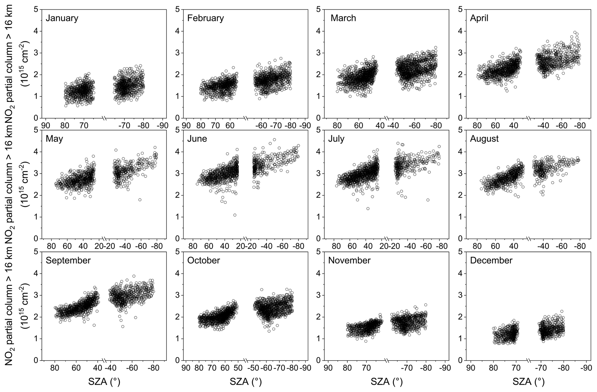
Figure 1 Retrieved NO₂ partial column above 16 km altitude measured at Zugspitze (black symbols) for every month with respect to SZA.

However, an observational counterpart, i.e., an analogous data set of experiment-based scaling factors describing the daytime increase in stratospheric NO_x, still does not exist due to the lack of reliable long-term data comprising the full daytime NO₂ and NO variability. To close this gap, in this paper we create a set of experiment-based scaling factors (SF_exp), analogous to the simulation-based scaling factors published by Strode et al. (2022). On the one hand, this data set should serve as a general set of data describing the NO_x daytime variability with respect to SZA for the given latitude (47° N) of our observation site. On the other hand, we would like to use the data set to validate the recently published model data for SF_sim(NO₂) (Strode et al., 2022) and unpublished model data for SF_sim(NO) (Sarah Strode, personal communication, 2023). For this SF_exp data set, we use the observational results described in Part 1 (Nürnberg et al., 2024), where a reliable long-term data set of NO₂ and NO partial columns above 16 km altitude above Zugspitze was created. As described above, these long-term data are retrieved from ground-based FTIR measurements and describe the daytime variability of stratospheric NO_x within time steps of minutes for every month of the year. The cutoff point at 16 km was chosen to avoid influences of variabilities near the tropopause and in the boundary layer upon the stratospheric partial column. Details are discussed in Part 1. It is outside the scope of this work to describe the strong and fast photochemistry at sunrise and sunset with SF_exp.

In Sect. 2, this paper (Part 2 of our companion paper) briefly describes the experimental setup and the resulting FTIR data taken from Part 1 (Nürnberg et al., 2024). In Sect. 3, the dependence on SZA for NO₂ and NO is shown, and the resulting daytime variations presented in detail in Part 1 are discussed briefly before the NO_x partial columns (>16 km) are converted into experiment-based scaling factors (SF_exp(NO₂) and SF_exp(NO)) in Sect. 4. Finally, the resulting SF_exp factors are compared qualitatively and quantitatively to SF_sim retrieved from model simulations.

2 FTIR data

All data of this study are retrieved from long-term ground-based FTIR solar absorption measurements at Zugspitze, Germany (47.42° N, 10.98° E; 2964 m a.s.l.). The high-altitude observatory at Zugspitze is located in the German Alps and can be regarded as a clean site without strong influences from pollution events in the boundary layer. The Bruker IFS 125HR spectrometer used in this study has been operating continuously since 1995 at Zugspitze. The experimental setup and retrieval strategy are described in the companion paper (Nürnberg et al., 2024). As described in Part 1, we used daily pressure and temperature profiles from the National Centers for Environmental Prediction (NCEP) interpolated to the measurement time. The temperature dependency of the data cannot be discussed in detail here, but it is very likely that the stratospheric temperature affects the NO_x concentration and therefore also the observed diurnal cycle. The pollution-filtered NO and NO₂ stratospheric partial columns (above 16 km altitude) derived in our Part 1 study serve as a basis for the experiment-based scaling factors created now in this Part 2 work. The data set comprises 6213 NO and 16 023 NO₂ partial columns measured at Zugspitze between 1995 and 2022.

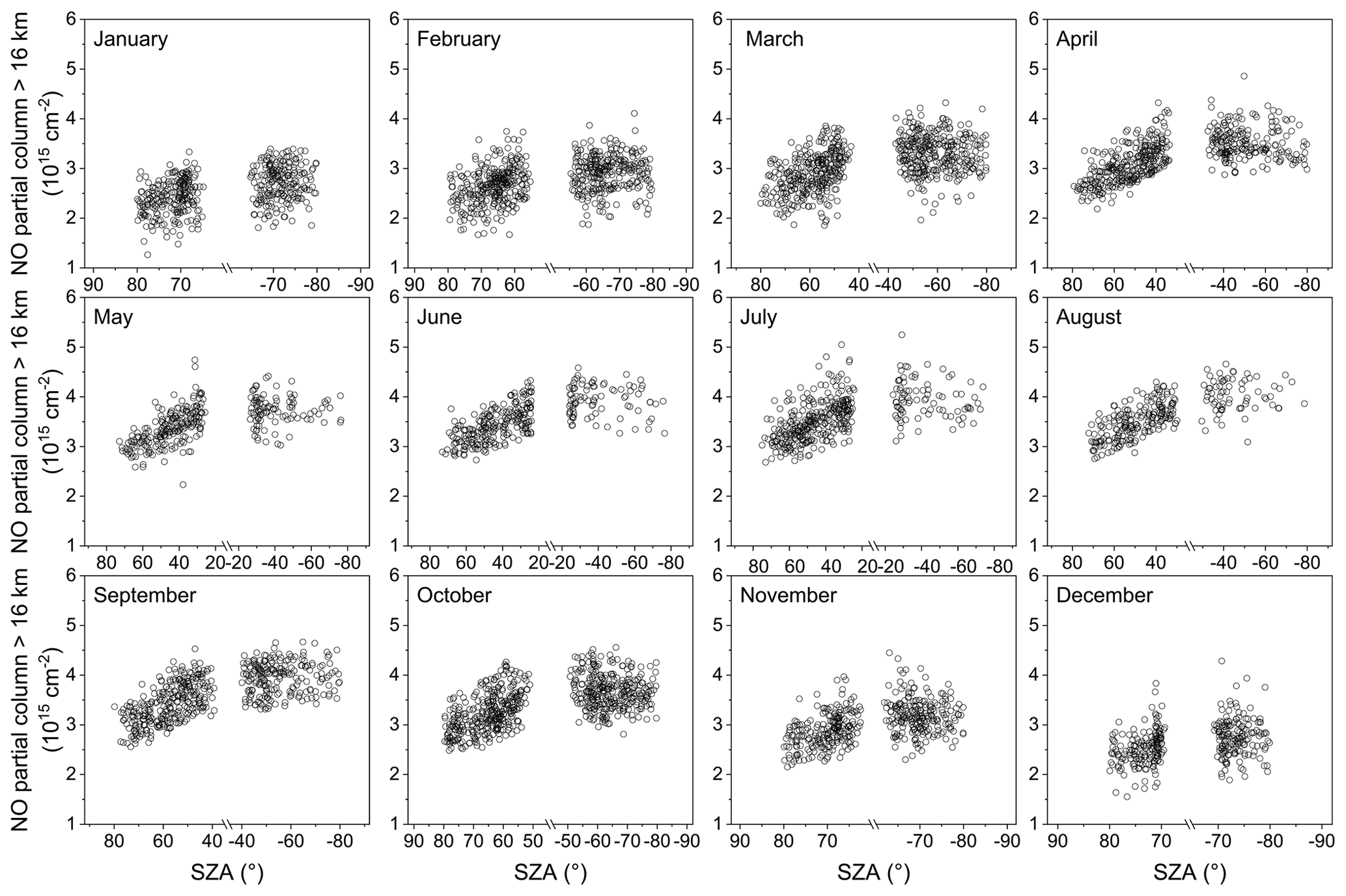
Figure 2 Retrieved NO partial column above 16 km altitude measured at Zugspitze (black symbols) for every month with respect to SZA.

3 Experimental data

NO_x stratospheric partial column dependence on SZA

Figure 1 shows the NO₂ stratospheric partial columns (black symbols) taken from Nürnberg et al. (2024) for every month as a function of SZA. Note this is the same data as shown in our Part 1 (Fig. 3 therein), which had been plotted as a function of local solar time. The x axis is interrupted for SZA values without observations in the respective month. Here, we define SZA to be positive in the morning from sunrise (SZA =90°) to local solar noon (respective minimum value dependent on the season) and to be negative in the afternoon between local solar noon and sunset (SZA $=-\mathrm{90}\mathit{°}$).

As already described and discussed in Part 1, the daytime increase in the NO₂ stratospheric partial column follows for every month a linear behavior from sunrise to sunset. Briefly, this behavior reflects the photolysis of the reservoir species HNO₃ and N₂O₅, resulting in a consecutive increase in NO₂ during daytime (Crutzen, 1970).

Similarly, Fig. 2 shows the NO stratospheric partial columns (black symbols) taken from the same work for every month with respect to SZA (Nürnberg et al., 2024). Note this is the same data as shown in our Part 1 (Fig. 5 therein) as a function of local solar time. Briefly, the data show the typical daytime increase in stratospheric NO described in the literature via model calculations (Dubé et al., 2020; McLinden et al., 2000) or shown experimentally (Zhou et al., 2021; Rinsland et al., 1984) for every month. Here, the photolysis of the reservoir species N₂O leads to a well-pronounced increase in the stratospheric NO concentration in the morning (Crutzen, 1970). After local solar noon, the shift in the NO₂–NO equilibrium, the increasing amount of O₃ and the solar elevation dependency of the involved photochemical reaction lead to a strong flattening of the daytime NO curve as a function of SZA in comparison to NO₂. This afternoon effect is more pronounced in the summertime (middle row) than in the rest of the year (Nürnberg et al., 2024).

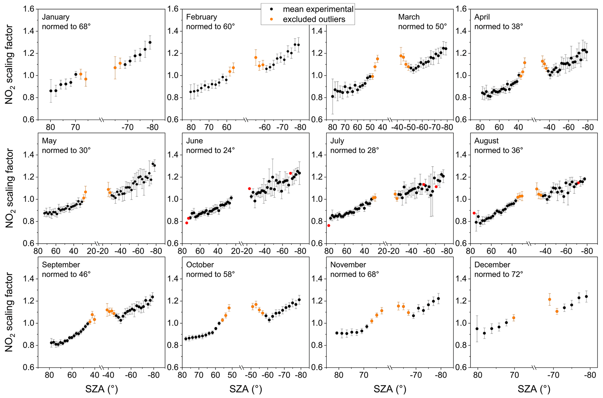
Figure 3 Calculated normalized NO₂ scaling factors SF_exp(NO₂) above 16 km altitude measured at Zugspitze (black; orange symbols are excluded outliers) for every month with respect to the SZA. The values represent the mean value within 2° SZA bins. The error bars represent 2 times the standard error of the mean (±2σ/√(n)) value. Values resulting from only one measurement point are shown in red without error bars.

4 Calculation of experiment-based scaling factors

A set of experiment-based scaling factors (SF_exp) analogous to the model-based scaling factors (SF_sim) published by Strode et al. (2022) was created as follows: the mean values for 2° bins of SZA of the stratospheric partial column (>16 km) were calculated. In a next step, these mean values were normalized to SZA =72° (which is the only value that is present in all monthly data sets), resulting in monthly SF_exp sets for NO₂ and NO shown in Figs. 3 and 4, respectively. These data reflect the daytime variation in stratospheric NO₂ and NO above Zugspitze, Germany. Values resulting from only one measurement point are shown in red without error bars.

SF_exp(NO₂) (Fig. 3, black and orange symbols) increases linearly throughout the day in each month, reflecting the increase in the stratospheric NO₂ concentration. There are two observations which can be pointed out here. First, the error bars in Fig. 3 (i.e., ±2 standard errors of the mean, ±2 SEM $=\pm \mathrm{2}\mathit{\sigma }/\surd \left(n\right))$ are independent of the season and are very small, reflecting a low scattering within the 2° SZA bins and enough averaging data points n. Second, in spring and autumn, at local solar noon (minimum SZA), a significant increase in SF_exp(NO₂) is visible. This effect can be understood as a boundary value problem being due to the relatively fast change in SZA and the NO₂ stratospheric partial column (seasonal variation) during the spring and autumn months, respectively. Here, the combination of both the SZA and the stratospheric partial column changes within 1 month results in an increased averaged NO₂ stratospheric partial column near the minimum SZA. The reason is that for SZA values below the minimum SZA at day 15 of each month, only partial columns from one half of the month can contribute to the average. Unfortunately, the stratospheric partial columns of this half deviate significantly from the monthly mean. Figure S1 in the Supplement illustrates this phenomenon using the NO₂ partial column above 16 km altitude. Here, the first half (red symbols) and the second half (blue symbols) of April are split up into two data sets underlining the described boundary value problem. At low SZA values, only blue data points sum up to the averaged values, considering only the second half of the month. Consequently, the partial column and, of course, the scaling factor increase artificially (pointed out by the blue arrow in the figure). This effect leads us to the exclusion of these data points (Fig. 3, orange symbols) below the minimum SZA reached at day 15 of the respective month. Another opportunity to face this problem would be the choice of a smaller time binning (e.g., 2 weeks, 10 d). However, this would (i) worsen the comparability to the simulation-based scaling factors and (ii) reduce the usable data base per time bin. The entire data set of SF_exp(NO₂) can be found in the Supplement Tables S1–S4.

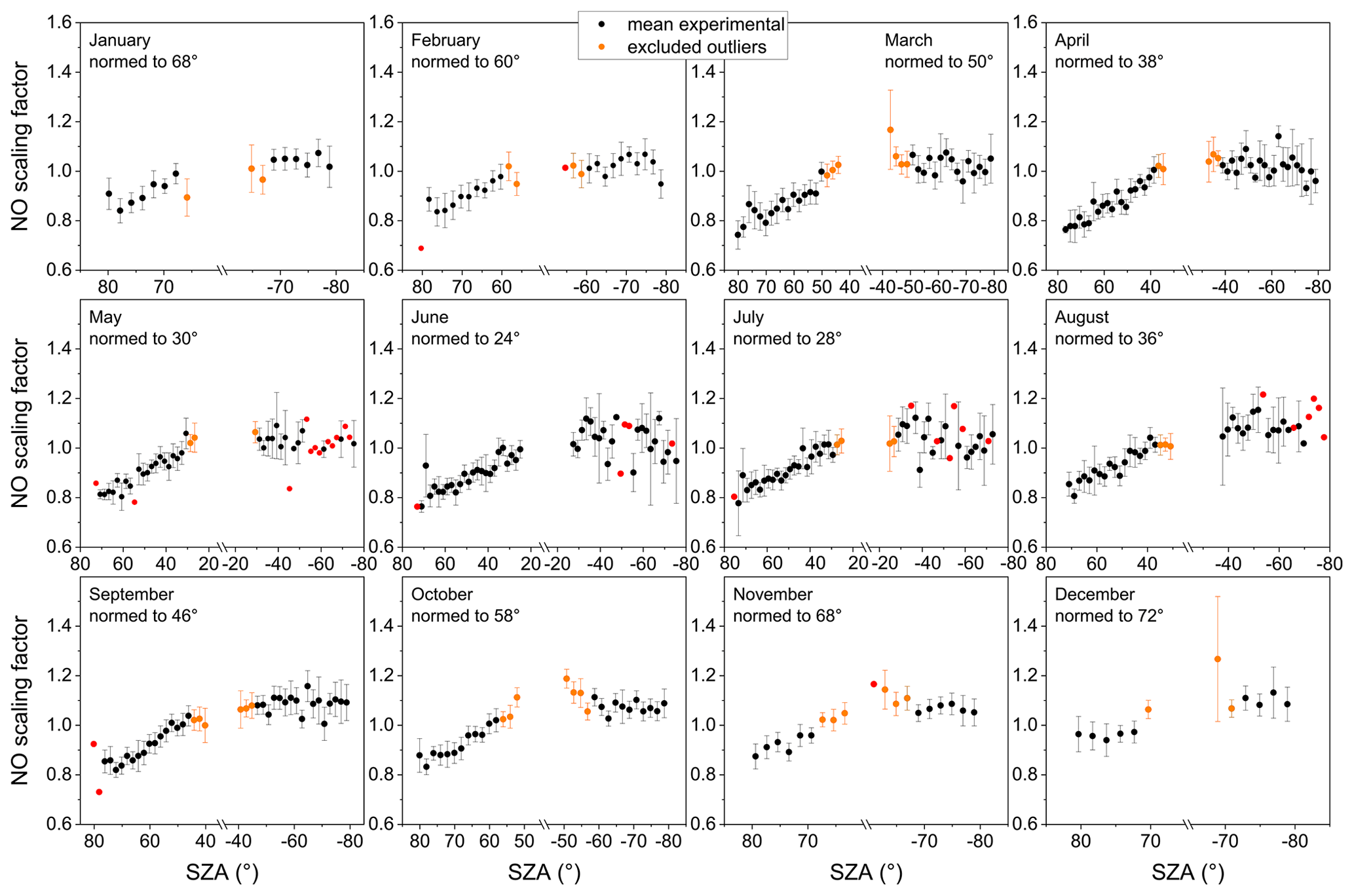
Figure 4 Calculated normalized NO scaling factors SF_exp(NO) above 16 km altitude measured at Zugspitze (black; orange symbols are excluded outliers) for every month with respect to SZA. The values represent the mean value within 2° SZA bins. The error bars represent 2 times the standard error of the mean ($\pm \mathrm{2}\mathit{\sigma }/\surd \left(n\right)$) value. Values resulting from only one measurement point are shown in red without error bars.

For SF_exp(NO) (Fig. 4, black and orange symbols), the difference in daytime increase in comparison to NO₂ is very well pronounced. Before local solar noon, SF_exp increases for every month linearly. After local solar noon, the described flattening of the increase is visible. Here, the NO stratospheric partial column stays almost constant within the scattering until sunset, independent of the season. The ±2 SEM error bars of SF_exp(NO) shown in Fig. 4 are also very small, but more values are excluded (red symbols) due to the availability of only one measurement point within the corresponding 2° SZA bin. This reflects the lower data base of the NO retrieval, originating from the use of another spectral micro-window for analysis. However, the small error bars underline that for most of the mean values, the data base is reliable. A similar but even less pronounced effect can be seen near local solar noon for SF_exp(NO), as described for NO₂. Here, the deviation from the visible trend in spring or autumn months is very small. However, for consistent data handling we also exclude the respective values (orange symbols) for SF_exp(NO) below the minimum SZA at each month on the 15th. The entire data set of SF_exp(NO) can be found in Tables S5–S8.

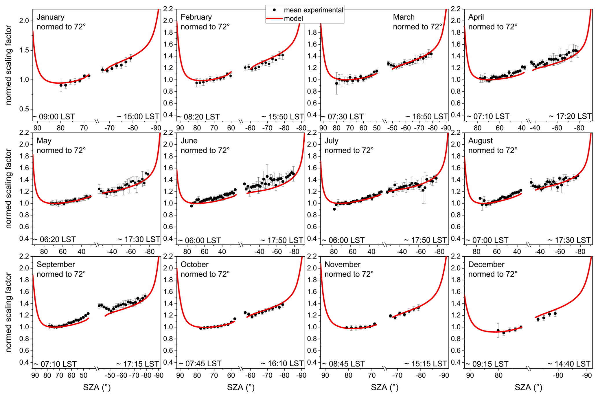
Figure 5 Calculated normalized NO₂ scaling factors SF_exp(NO₂) above 16 km altitude measured at Zugspitze (black) and recalculated normalized NO₂ scaling factors SF_sim(NO₂) above 16 km altitude (red line) for every month with respect to SZA. The experimental values represent the mean value within 2° SZA bins. The error bars represent 2 times the standard error of the mean ($\pm \mathrm{2}\mathit{\sigma }/\surd \left(n\right))$ value.

5 Model comparison of NO_x scaling factors

In the previous section, we created experiment-based averaged monthly scaling factors SF_exp for NO₂ and NO describing the daytime variation in stratospheric NO_x concentration above Zugspitze, Germany. Next, we compare the discussed results for SF_exp to model-based scaling factors SF_sim for NO₂ published by Strode et al. (2022) and for NO calculated from the same GEOS-GMI model simulation as the NO₂ scaling factors. Details of the GEOS model simulation with GMI chemistry (Duncan et al., 2007; Strahan et al., 2007; Nielsen et al., 2017) are described in Strode et al. (2022) and references therein. The model parameters and the analysis method can be found in the literature (Strode et al., 2022). The given scaling factors SF_sim(NO₂) and SF_sim(NO) are available for 146 levels between 6 and 78.5 km altitude in a 0.5 km grid and are normalized to SZA =90° (sunrise). For a better comparison of the experiment and model, we calculated mean values for SF_sim which also represent the stratospheric partial column above 16 km altitude. In order to do so, for each model level z, SF_sim(z) was weighted to the mean monthly partial column profile of the given NO_x retrieval at z, and SF_sim(>16 km) was obtained via averaging over SF_sim(16 km) to SF_sim(78.5 km). Furthermore, SF_sim(>16 km) was normalized to SZA =72° (rather than sunrise/sunset), as done for SF_exp in Sect. 4.

SF_sim(NO₂) and SF_sim(NO) are additionally shown in Figs. 5 and 6, respectively (red line). At first glance, SF_exp (black symbols) and SF_sim (red line) fit together very well, and the model data follow the experimental daytime variation for both NO₂ and NO.

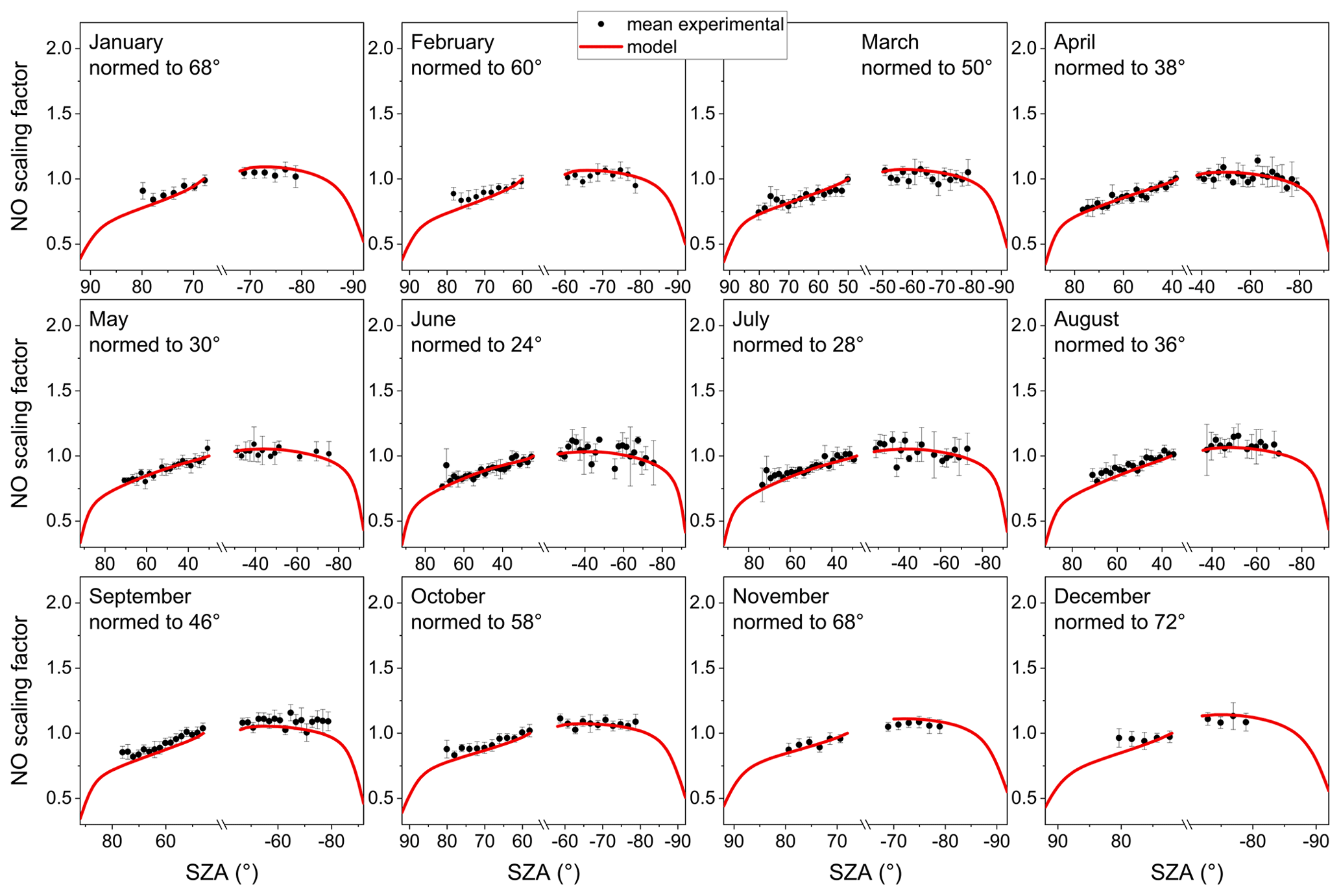
Figure 6 Calculated normalized NO scaling factors SF_exp(NO) above 16 km altitude measured at Zugspitze (black) and recalculated normalized NO scaling factors SF_sim(NO) above 16 km altitude (red line) for every month with respect to SZA. The experimental values represent the mean value within 2° SZA bins. The error bars represent 2 times the standard error of the mean ($\pm \mathrm{2}\mathit{\sigma }/\surd \left(n\right))$ value.

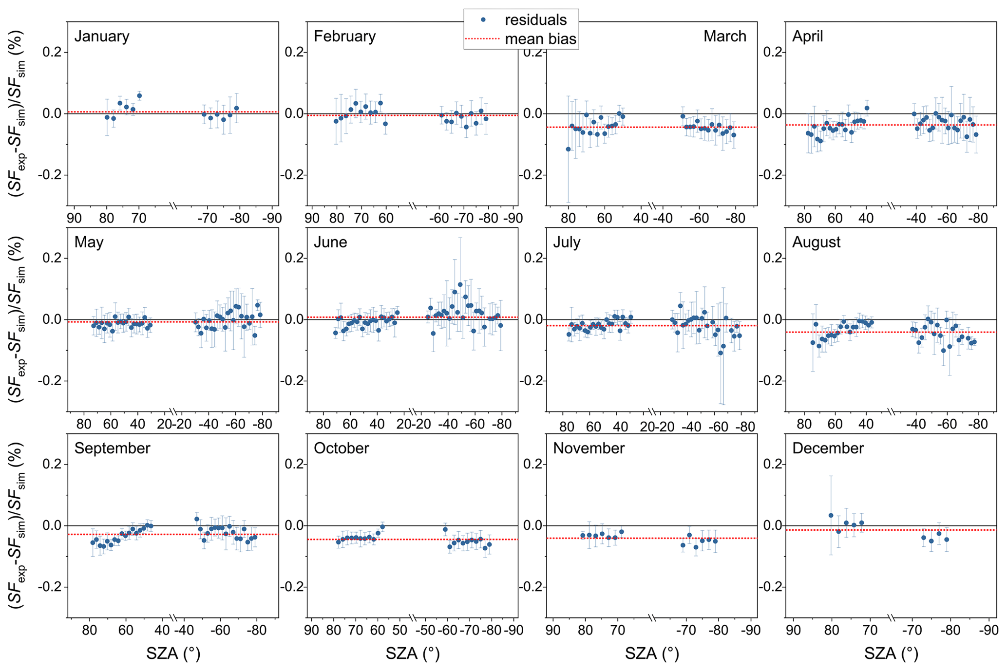
Figure 7 Calculated residuals (SF_exp–SF_sim)/SF_sim between the experimental normalized mean NO₂ scaling factors SF_exp and the simulated normalized NO₂ scaling factors SF_sim, interpolated to the respective SZA for every month with respect to SZA. The error bars represent 2 times the propagated standard error of the mean ($\pm \mathrm{2}\mathit{\sigma }/\surd \left(n\right))$ of the experimental value. The mean bias over all SZAs is shown in red.

Quantitative evaluation

For the quantitative evaluation of the model comparison, the residuals between the experiment and model (SF_exp–SF_sim)/SF_sim are calculated for SF(NO₂) and SF(NO) and are shown in Figs. 7 and 8, respectively. Additionally, the mean bias per month is shown as a mean value over all SZAs (dotted red line).

The residuals of SF(NO₂) (Fig. 7) show over the whole year very good agreement between the experiment and model within ±0.2 %, reflecting the high quality of the GEOS-GMI simulation at midlatitudes. Significant differences between the experiment and model are visible only for a few months. For April, August and September, the morning increase in NO₂ is less pronounced in the model, leading to a significant deviation from the experimental values and an underestimation of the experiment-based scaling factors SF_exp at noon. However, the experimental values describing the stratospheric NO₂ variability can also be influenced by tropospheric variations because the NO₂ partial column used cannot be treated as completely independent of the tropospheric partial column (see Nürnberg et al., 2024). Furthermore, the model data have higher uncertainties during twilight, which can lead to deviations from the experiment (Alvanos and Christoudias, 2019).

Table 1 Calculated mean bias of residuals ([SF_exp–SF_sim]/SF_sim) for every month between the experiment and simulations for NO₂ and 2 times the standard error of the mean ($\mathrm{2}\mathit{\sigma }/\surd \left(n\right))$ of this value.

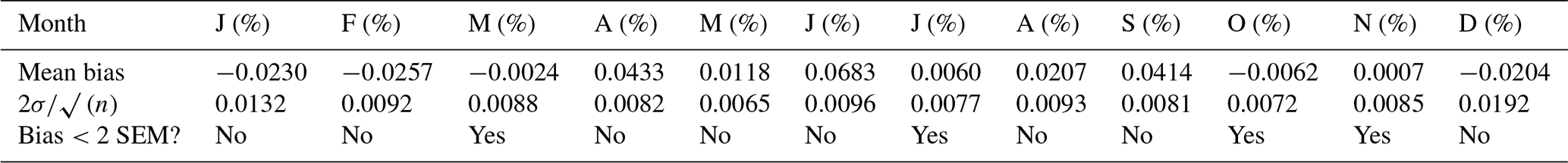
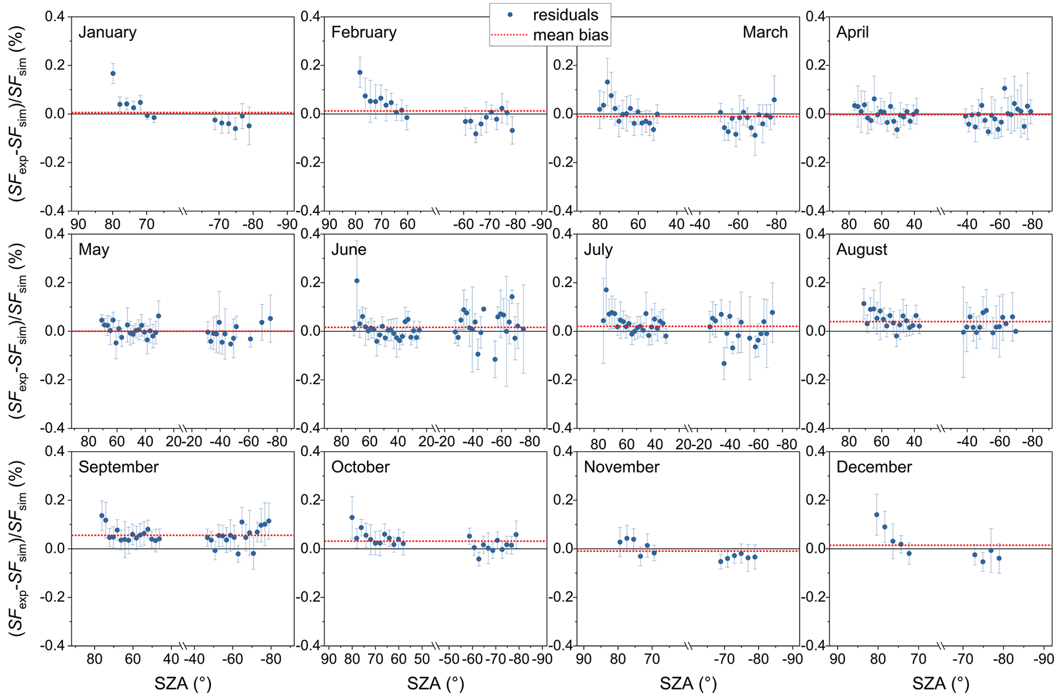
Figure 8 Calculated residuals ([SF_exp–SF_sim]/SF_sim) between the experimental normalized mean NO scaling factors SF_exp and the simulated normalized NO scaling factors SF_sim, interpolated to the respective SZA for every month with respect to SZA. The error bars represent 2 times the propagated standard error of the mean ($\pm \mathrm{2}\mathit{\sigma }/\surd \left(n\right))$ of the experimental value. The mean bias over all SZAs is shown in red.

Table 1 shows the mean bias (see also Fig. 7, dotted red line) for every month calculated from the residuals shown in Fig. 7 together with 2 times the SEM ($\mathrm{2}\mathit{\sigma }/\surd \left(n\right)$). Unfortunately, due to the small values of 2 SEM of 0.0065 % to 0.0192 % for most of the months (except March, July, October, November), 2 SEM is smaller than the mean bias. Therefore, when taking 2 SEM as a quantitative indicator, SF_exp and SF_sim agree only in 4 months within the margin of error. However, when considering the mean deviation between the experiment and model of below $\left|\mathrm{0.068}\mathit{\%}\right|$ per month, we can state that the model data published by Strode et al. (2022) reflect the experimental values retrieved from solar FTIR measurements at midlatitudes sufficiently well.

A very similar behavior can be obtained for SF(NO) (Fig. 8). With a maximum deviation of ±0.2 %, the agreement between the experiment and model is very similar, as seen for NO₂. However, it is remarkable that for the months with the highest SZA (January, February), the first data points after sunrise for which measurements exist (high-SZA region) deviate significantly from 0. Compared to Fig. 6, the experimental values in this region do not seem to follow the continuous increase expected from model descriptions. Here, an error source of the experimental data can be the wide range in photochemical regimes along the line of sight of the FTIR slant column measurements at high SZA: high up in the atmosphere, the sun is already well above the horizon, so there has already been significant NO production, while lower down the atmosphere is still much darker, and NO levels are still lower. The FTIR retrieval leads to an averaging over these effects because NO slant columns along the line of sight are retrieved from the solar measurements, and these are then converted to vertical column densities using a simple cos(SZA) air mass correction.

Furthermore, the NO increase in the morning is more pronounced in the model, leading to a significant deviation from the experimental values and an overestimation of the experiment-based scaling factors SF_exp at noon. In the same manner as discussed before for NO₂, the experimental values describing the stratospheric NO variability can be influenced by tropospheric variations because the NO partial column used cannot be treated as completely independent of the tropospheric partial column (see Nürnberg et al., 2024). Consequently, the lower-stratospheric partial column in the morning is more influenced by the tropospheric partial column than in the evening.

Table 2 Calculated mean bias of residuals ([SF_exp–SF_sim]/SF_sim) for every month between the experiment and simulations for NO and 2 times the standard error of the mean ($\mathrm{2}\mathit{\sigma }/\surd \left(n\right))$ of this value.

In the same way as done for NO₂, the mean bias (see also Fig. 8, dotted red line) and 2$\mathit{\sigma }/\surd \left(n\right)$ (2 SEM) are calculated and are shown in Table 2 for the NO residuals. Here, better agreement between the experiment and model can be quantified. For 6 months (January, June, September, October, November, December) the mean bias is smaller than 2 SEM, indicating agreement between the experiment and model within the error bars. Nevertheless, this observation not only reflects better agreement between the experiment and model but can also be explained by a higher scattering of the residuals, leading to a higher SEM. This can be confirmed when comparing the values for 2 SEM given in Tables 1 and 2. With a mean 2 SEM of the residuals over all months of 0.0096 % for NO₂ and 0.0185 % for NO, the residual scattering with a similar n and a similar mean bias of 0.02 % is 2 times larger for NO.

In conclusion, the quantitative comparison of the experimental-derived scaling factors SF_exp and the scaling factors derived from model simulations SF_sim for NO₂ and NO showed very good agreement between both data sets, with a mean bias between the experiment and model of only 0.02 % over all months, underlining the quality of the model data at midlatitudes and the reliability of the retrieved experiment-based scaling factors.

6 Summary and conclusions

In this work, we reanalyzed an experimental long-term data set from solar FTIR measurements over 25 years of measurement at Zugspitze (47.42° N, 10.98° E; 2964 m a.s.l.), Germany, published in a companion paper (Part 1, Nürnberg et al., 2024). We present for the first time experiment-based scaling factors SF_exp as a function of the solar zenith angle (SZA), representing monthly daytime NO₂ and NO variabilities in the stratosphere (>16 km altitude) within time steps of minutes. SF_exp is a measure of the variability of the NO_x partial column above 16 km altitude in comparison to local solar noon. We calculated SF_exp from the time-dependent monthly NO_x partial columns (published in Part 1) by averaging over SZA bins of 2° and a normalization to SZA=72°. The resulting values of SF_exp(NO₂) and SF_exp(NO) reflect the expected daytime variability of NO₂ and NO described in Part 1 very well (Nürnberg et al., 2024). Only the boundary values in spring and autumn months deviate significantly due to the relatively fast change in the minimum SZA during these months, which influences the average value. Neglecting these values leads to two reliable experiment-based data sets for SF_exp(NO₂) and SF_exp(NO). Furthermore, we used these new experiment-based data sets to validate recently published simulation-based scaling factors SF_sim(NO₂) (Strode et al., 2022) and recently calculated simulation-based scaling factors SF_sim(NO) from a global study representing a similar latitude (47° N). Comparing the experiment and model simulation, we find excellent agreement for stratospheric NO₂ and NO daytime variabilities, with a mean bias of the modulus over all months and SZA of only 0.02 %, with no significant deviating trends for boundary values. These results underline the quality of recent multi-dimensional model simulations of stratospheric trace gases, representing experimental data very well. Additionally, we showed that ground-based FTIR measurements can provide reliable information about stratospheric NO_x variability within time steps of minutes, which can serve as a good basis for the validation of global model simulations and can therefore help to further optimize satellite validations.

The analysis method for retrieving stratospheric NO₂ and NO partial columns over Zugspitze, Germany, published in Part 1 (Nürnberg et al., 2024), combined with the generalization of this data by calculating unitless scaling factors (SFs) and the validation of recently published model data in this paper (Part 2), can be seen as a useful tool for the further validation and correction of global model and satellite data. This approach can be taken for any ground-based FTIR spectrometer generating a global set of experiment-based stratospheric NO₂ and NO partial columns or scaling factors SF_exp(NO₂) and SF_exp(NO).