Stratospheric aerosol size reduction after volcanic eruptions

The stratospheric aerosol layer plays an important role in the radiative balance of Earth primarily through scattering of solar radiation. The magnitude of this effect depends critically on the size distribution of the aerosol. The aerosol layer is in large part fed by volcanic eruptions strong enough to inject gaseous sulfur species into the stratosphere. The evolution of the stratospheric aerosol size after volcanic eruptions is currently one of the biggest uncertainties in stratospheric aerosol science. We retrieved aerosol particle size information from satellite solar occultation measurements from the Stratospheric Aerosol and Gas Experiment III mounted on the International Space Station (SAGE III/ISS) using a robust spectral method. We show that, surprisingly, some volcanic eruptions can lead to a decrease in average aerosol size, like the 2018 Ambae and the 2021 La Soufrière eruptions. In 2019 an intriguing contrast is observed, where the Raikoke eruption (48^∘ N, 153^∘ E) in 2019 led to the more expected stratospheric aerosol size increase, while the Ulawun eruptions (5^∘ S, 151^∘ E), which followed shortly after, again resulted in a reduction in the values of the median radius and absolute distribution width in the lowermost stratosphere. In addition, the Raikoke and Ulawun eruptions were simulated with the aerosol climate model MAECHAM5-HAM. In these model runs, the evolution of the extinction coefficient as well as of the effective radius could be reproduced well for the first 3 months of volcanic activity. However, the long lifetime of the very small aerosol sizes of many months observed in the satellite retrieval data could not be reproduced.

1 Introduction

The variability in stratospheric sulfate aerosol is still not well understood, and the question of whether they increase in size after large SO₂ injections, e.g., by volcanic eruptions reaching the stratosphere, is one of the most important research questions of recent years (Robock, 2015). The size of stratospheric aerosol is a crucial factor for their effect on the lifetime of the aerosol and atmospheric chemistry (Deshler, 2008; Kremser et al., 2016), e.g., on ozone levels, as well as for their effect on the radiative balance of Earth and therefore their net cooling effect on Earth's surface (Lacis et al., 1992). The expectation of how the size distribution of stratospheric aerosol changes after volcanic injections of sulfurous gases into the stratosphere is still largely based on studies on the Mt. Pinatubo eruption in 1991, which led to a significant increase in the size of stratospheric sulfate aerosol (Bingen et al., 2004; Deshler et al., 2003; Deshler, 2008). It was the largest volcanic eruption observed with satellite instruments to date and had a strong impact on the stratospheric aerosol distribution. Because of this, the observations of this eruption are widely used to evaluate aerosol microphysical models (Timmreck, 2001; Aquila et al., 2012; Niemeier et al., 2009; Sukhodolov et al., 2018; Quaglia et al., 2023).

On the other hand, many much smaller volcanic events have been observed by space-based instruments over the past 40 years. Those smaller eruptions may have different effects on the stratospheric aerosol size. In this work, as a part of the research project VolImpact (von Savigny et al., 2020), we investigate the evolution of the stratospheric aerosol size after the eruptions of four volcanoes within the mission time of the Stratospheric Aerosol and Gas Experiment III mounted on the International Space Station (SAGE III/ISS), namely Ambae (15^∘ S, 168^∘ E), Raikoke (48^∘ N, 153^∘ E), Ulawun (5^∘ S, 151^∘ E) and La Soufrière (13^∘ N, 61^∘ W).

Using the remote sensing data set of the SAGE III instrument mounted on the International Space Station (SAGE III/ISS) we retrieved the size distribution parameters of monomodal log-normal size distributions with a robust multi-wavelength method. We show that while the Raikoke eruption had an increasing effect on the average aerosol size, the Ambae, Ulawun and La Soufrière eruptions led to an unexpected and considerable decrease. We also simulated the Raikoke and Ulawun eruptions using the aerosol climate model MAECHAM5-HAM (short ECHAM) (Stier et al., 2005; Niemeier et al., 2009), in order to investigate whether it can be used to identify and understand the main dynamical and microphysical factors controlling the aerosol size evolution caused by the eruptions. This is also relevant for the modeling community, since previous model studies usually concentrated on the long-term development of the particle size (Sukhodolov et al., 2018) instead of on the first few months of its evolution.

In Sect. 2 the instrumental and modeling data sets used and the methods employed are described. In Sect. 3 an overview over the three periods of volcanic activity that are being investigated is given, followed by the presentation of the spatial and temporal evolution of the retrieved aerosol size distribution parameters for those periods (Sect. 4), which is discussed in Sect. 5. Finally, in Sect. 6 model simulations of aerosol extinction and size for the Raikoke and Ulawun eruptive period are presented and compared to the SAGE III/ISS retrieval data.

2 Instruments and methodology

2.1 SAGE III/ISS instrument

The SAGE III/ISS instrument is the latest successor of the previous SAM II (Stratospheric Aerosol Measurement), SAGE I, SAGE II and SAGE III Meteor-3M satellite experiments and aims at the investigation of the stratosphere and upper troposphere. Its mission started in June 2017 with its measurements still ongoing at the time of writing. On board the ISS, which has an orbital inclination of 51.6^∘ and orbits Earth in about 92 min, the instrument performs lunar and solar occultation measurements. Only the latter are used in this work. Due to the platform's orbit SAGE III/ISS observes roughly 15 sunrise and 15 sunset events in 24 h. Sunrise and sunset measurements are taken at different latitudes, and these latitudes oscillate roughly between 70^∘ N and 70^∘ S with a period of around 2 months (Cisewski et al., 2014).

Through the measurement of the solar radiation attenuated by atmospheric constituents the SAGE III/ISS data set provides information on gases like ozone and water vapor as well as on aerosol. Aerosol extinction coefficients are provided at nine spectral channels between 384 and 1544 nm on a 0.5 km grid from Earth's surface up to 45 km altitude. The spectral resolution of the first eight channels between 384 and 1020 nm, which are all covered by a CCD array, is 1–2 nm. The 1544 nm channel is detected by an indium gallium arsenide (InGaAs) infrared photodiode and has a bandwidth of about 30 nm. In this work, version 5.21 of the SAGE III/ISS level 2 data is used (SAGE III Science Team, 2021).

Advantages of using aerosol extinction data from the SAGE III/ISS satellite solar occultation measurements are firstly that there is no need to make assumptions on the particle size distribution (PSD) to retrieve the extinction coefficients in the first place. Secondly, the Sun provides a strong signal, benefitting the signal-to-noise ratio of the data product. Data are provided with a high vertical resolution. Additionally, since the measurements of every sunset or sunrise event are calibrated with corresponding direct solar irradiance measurements between 100 and 300 km, the data set is relatively unaffected by changes in the instrument over time. On the other hand the spatial and temporal coverage is low compared to, e.g., satellite limb measurements. This is because in a single day only around 30 profiles are obtained and only a narrow latitude range is covered. Still, compared to ground-based measurements, an almost global coverage is possible within 1–2 months. Therefore, an analysis of the spatial and temporal evolution of quantities derived from the SAGE III/ISS measurements is feasible (see Sects. 3 and 4) (SAGE III Science Team, 2022).

2.2 Particle size retrieval method

The method that was used for the retrieval of the stratospheric aerosol particle size from the SAGE III/ISS data set has been described in detail in Wrana et al. (2021). Therefore, the size distribution parameter retrieval method employed will only be described briefly here.

A monomodal log-normal shape of the size distribution for stratospheric aerosol is assumed, which is expressed mathematically as follows:

$$\begin{array}{}\text{(1)}& n\left(r\right)={\displaystyle \frac{\mathrm{d}N\left(r\right)}{\mathrm{d}r}}={\displaystyle \frac{N_{\mathrm{0}}}{\sqrt{\mathrm{2}\mathit{\pi }}\cdot r\cdot \ln \mathit{\sigma }}}\cdot \exp \left(-{\displaystyle \frac{{\ln }^{\mathrm{2}}(r/r_{\mathrm{med}})}{\mathrm{2}{\ln }^{\mathrm{2}}\mathit{\sigma }}}\right),\end{array}$$

with N₀ being the total number density, r_med being the median radius and σ being the distribution width of the particle size distribution. These parameters needed to be retrieved.

The aerosol is assumed to be composed of a solution of 75 % H₂SO₄ and 25 % H₂O. Furthermore, stratospheric aerosol is assumed to be spherical in shape; thus the Mie theory can be applied. The possible values of the parameters to be retrieved are assumed to lie between 1 and 1000 nm for the median radius and 1.05 and 2.0 for the distribution width.

Before their use in the retrieval process, the extinction coefficients provided in the SAGE III/ISS data set were smoothed over altitude using a 1–2–1 smoothing scheme, aligning the version 5.21 data set with that of version 5.1, where a similar smoothing of the data was inherent. Two extinction ratios using a total of three wavelengths (449 nm : 756 nm and 1544 nm : 756 nm) are used to retrieve the median radius and the distribution width σ. Using a Mie code (Mie scattering routines, 2018) these extinction ratios were calculated for all combinations of a median radius value between 1 and 1000 nm in 1 nm increments and a distribution width value between 1.05 and 2.0 in steps of 0.1. The real parts of the refractive indices at the wavelengths used were calculated from Palmer and Williams (1975) using Lorentz–Lorenz corrections. These corrections have been described by Steele and Hamill (1981) and were necessary to obtain refractive indices at typical lower-stratospheric temperatures. The results of the Mie calculations are then used as a lookup table, since a given combination of the median radius and σ can be related to a specific combination of the calculated extinction ratios at 449 nm : 756 nm and 1544 nm : 756 nm. Forming extinction ratios at the same wavelengths from the SAGE III/ISS extinction coefficient data set, both size distribution parameters can then be retrieved by means of interpolation using the lookup table. More details are provided in Wrana et al. (2021).

The effective radius which is used for the comparison to the model simulations in Sect. 6 is calculated from the median radius and distribution width with the following relation:

$$\begin{array}{}\text{(2)}& r_{\mathrm{eff}}=r_{\mathrm{med}}\cdot \exp \left({\displaystyle \frac{\mathrm{5}}{\mathrm{2}}}\cdot {\ln }^{\mathrm{2}}\left(\mathit{\sigma }\right)\right).\end{array}$$

Also, an accuracy parameter a as defined by Wrana et al. (2021), which is calculated from the distance between the curves of the lookup table and the error bars of the extinction ratios calculated from the SAGE III/ISS extinction coefficients, is used to exclude noisy data in the retrieved quantities shown in this work.

2.3 ECHAM model

The simulations of the Raikoke and Ulawun volcanic eruptions (see Sect. 6) were performed using MAECHAM5-HAM. ECHAM5 (Giorgetta et al., 2006), a general circulation model, was used in its middle atmosphere (MA) version, with a horizontal resolution of about 1.8^∘. It has a spectral truncation at wavenumber 63 (T63), with 95 vertical layers up to 0.01 hPa (about 80 km). To achieve realistic wind and transport conditions, a nudging of the large wavenumbers of the model to ERA5 reanalysis data was performed (Hersbach et al., 2020).

The aerosol microphysical model HAM (Stier et al., 2005) is interactively coupled to ECHAM. HAM includes the simulation of the oxidation of sulfur and sulfate aerosol formation, including nucleation, accumulation, condensation and coagulation processes. Above the tropopause, a simple stratospheric sulfur chemistry was considered (Timmreck, 2001; Hommel et al., 2011) using prescribed chemical species of OH, NO₂ and O₃. In the simulations, the sulfate aerosol is radiatively active for both shortwave and longwave radiation and coupled to the radiation scheme of ECHAM. The model setup and the setup of the distribution width is described in Niemeier et al. (2009) and Niemeier and Timmreck (2015), respectively. The parametrization of nucleation processes has been updated according to Määttänen et al. (2018), which slightly increased particle nucleation in the model.

2.4 TROPOMI instrument

For the comparison of model to observations data in Sect. 6 the emitted SO₂ masses of the 2019 Raikoke and Ulawun eruptions were estimated from TROPOMI (TROPOspheric Monitoring Instrument) measurements on board of the Sentinel-5 Precursor satellite. The data product used in this study assumes the SO₂ profile as a 1 km thick box filled with SO₂ and centered at 15 km altitude. We defined a grid with a latitude–longitude resolution of 0.1^∘ × 0.1^∘ from 30^∘ N to 30^∘ S and 110^∘ E to 100^∘ W. For the June and August 2019 eruptions of Ulawun, only SO₂ total vertical column data with a solar zenith angle less than 70^∘ (Theys et al., 2021) and with values less than 1000 mol m⁻² were used. The vertical columns were multiplied by the SO₂ molar mass in order to obtain an SO₂ mass loading in units of grams per square meter. Different thresholds of either 0 or 0.05 g m⁻² were applied to distinguish the volcanic signal from the background. The data were averaged for each grid segment, and the SO₂ mass in units of grams was determined for each segment. Since some orbits spatially overlap, 14 consecutive orbits were bundled into a batch that covered approximately 24 h and averaged for each grid segment of the batch. The SO₂ mass in all grid segments of a batch were summed up to finally receive the total SO₂ mass per batch. Depending on the threshold, estimates for the SO₂ mass were 0.12–0.16 Tg for the June 2019 eruption and 0.18–0.2 Tg for the August eruption. The SO₂ mass emitted by the Raikoke eruption in June 2019 was calculated using no threshold with no restriction on the solar zenith angle but with the requirement that the quality value needs to be larger than 0.5. This is described in more detail in Muser et al. (2020) and resulted in an SO₂ mass estimate of 1.37 Tg.

3 SAGE III/ISS timeline

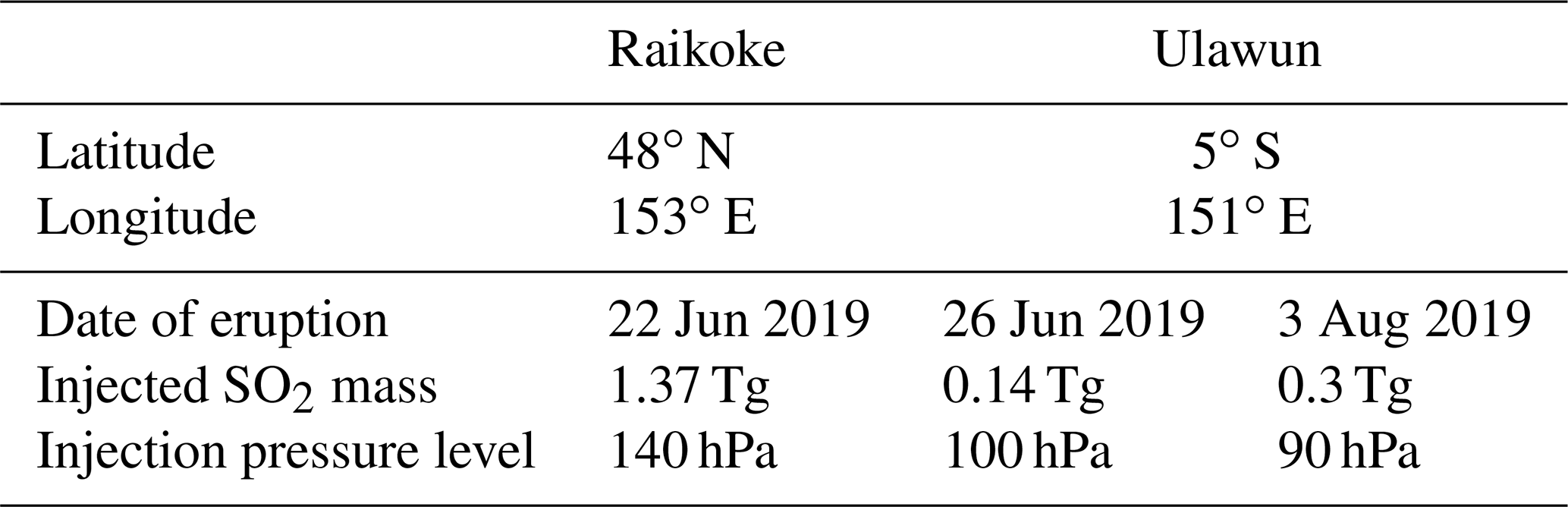
In this section an overview of the volcanic eruptions investigated in this work is given. Three main periods of volcanic activity will be looked at: the Ambae eruptions of 2018, the Raikoke and Ulawun eruptions of 2019, and the La Soufrière eruption of 2021. Table 1 summarizes information on the most important eruptions and eruptive phases in that time frame, important insofar as the eruptions were explosive enough to inject SO₂ directly into the stratosphere.

Table 1 Information related to the most important volcanic eruptions and eruptive phases leading to direct injections of SO₂ into the lower stratosphere in the time period discussed in this work and covered by the SAGE III/ISS instrument, i.e., 2018–2021. Sources: Muser et al. (2020), Kloss et al. (2020), Kloss et al. (2021), Joseph et al. (2022) and Bruckert et al. (2023).

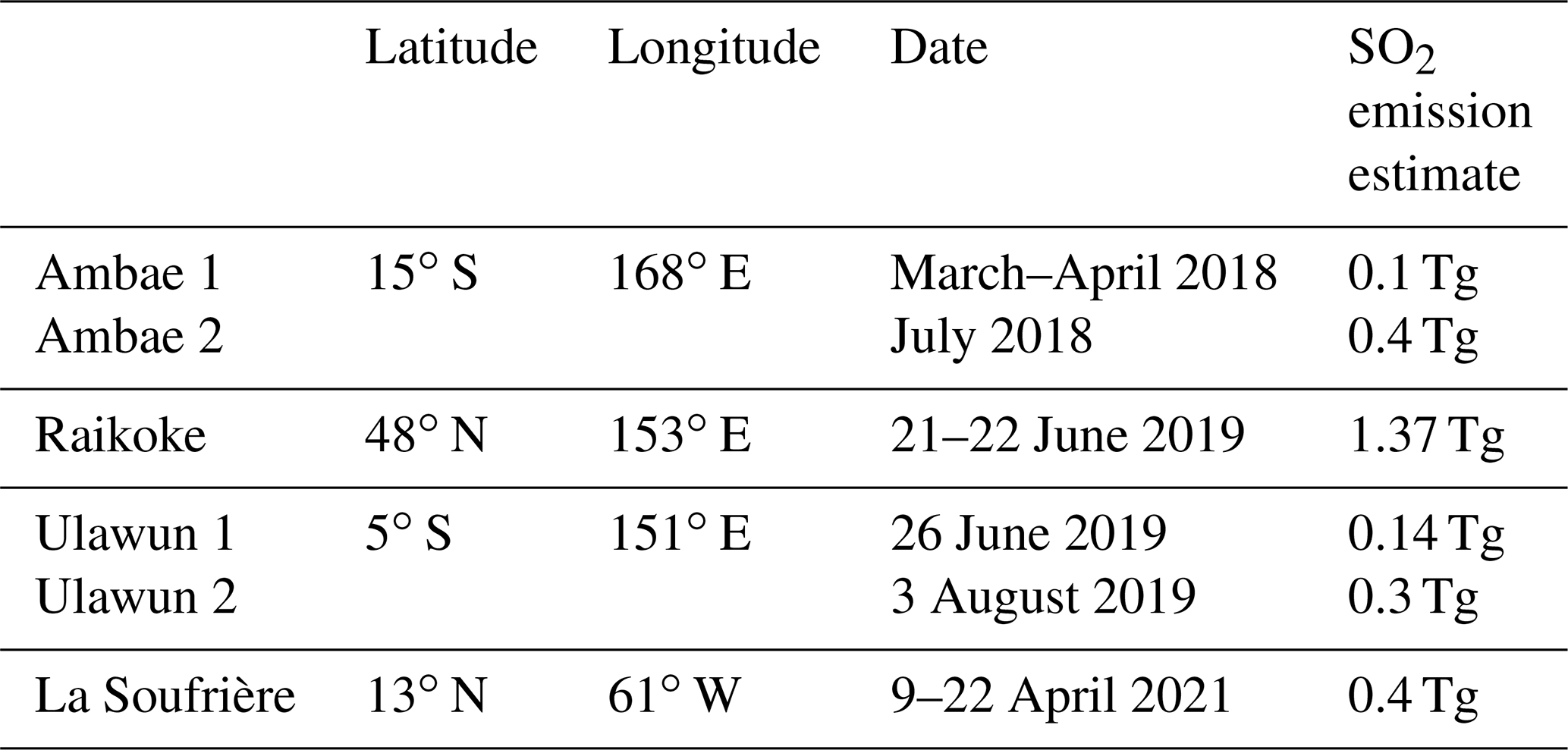
Figure 1 gives an overview of the evolution of the extinction coefficient at 449 nm from the SAGE III/ISS data in the tropics to give a sense of the temporal order of the volcanic eruptions investigated in this work. Daily zonal averages between 30^∘ S and 30^∘ N are shown for the time between 2018 and early 2022. Darker colors indicate higher values. The panel above shows which latitude the measurements of the averaged profiles beneath correspond to, due to the latitudinal shift in the SAGE III/ISS measurements. Dashed red lines indicate the dates of volcanic eruptions, whose signatures can be seen as darker colors in the contour plot. Since the latitudes of the SAGE III/ISS occultation measurements change from day to day, there are gaps in the sampling of any particular latitude band, such as the tropics in this case, which explains the time gaps in the color plots.

We observe that the aerosol extinction coefficient at 449 nm is around 10⁻⁴ km⁻¹ in the main aerosol layer from the start of the mission until the April 2018 eruption of Ambae. As would be expected, extinction increases in the lower stratosphere after each individual volcanic eruption. As described by Vernier et al. (2011), the new aerosol in the lower tropical stratosphere rises slowly to higher altitudes in a manner that mimics the water vapor “tape recorder”.

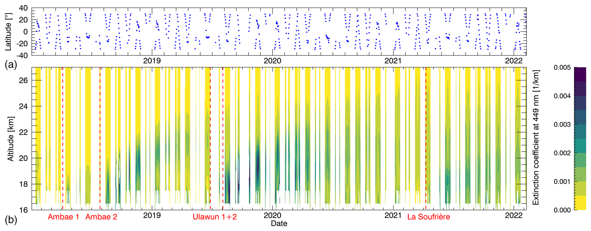
Figure 1 (b) Daily zonal means of the extinction coefficient at 449 nm between 30^∘ S and 30^∘ N. (a) Geolocations of the SAGE III/ISS solar occultation measurements used. Dashed vertical lines indicate volcanic eruptions that happened during the depicted time frame and reached the stratosphere.

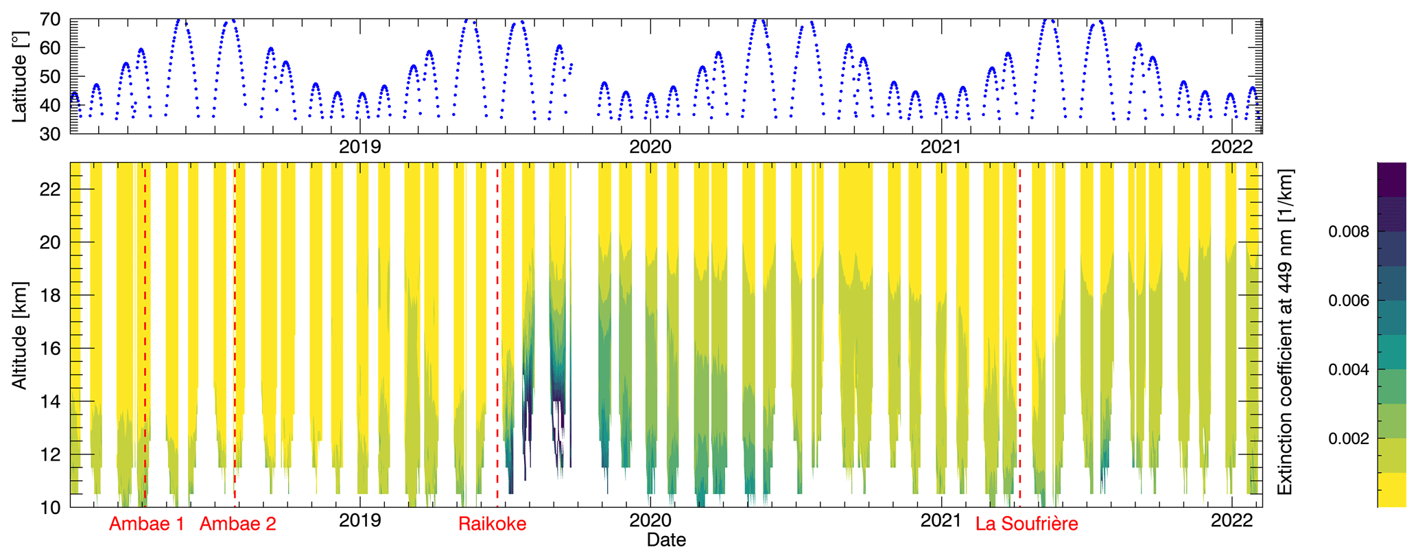
Similarly to Fig. 1, Fig. 2 shows the extinction coefficient at 449 nm but for latitudes between 35 and 70^∘ N. Due to the lower tropopause height here, which also results in the stratospheric aerosol layer residing at lower altitudes, a different altitude window is shown. Notice also the difference in the color scale value range. Here, the signature of the Raikoke eruption, which was the strongest of the eruptions discussed in this work, dominates. It has to be noted that, in this region, as well as in Fig. 1, the signatures of the Raikoke and Ulawun eruptions cannot be clearly separated from each other. Although the perturbations are much lower, it can be seen that the aerosol plumes of the Ambae and La Soufrière eruptions also reach the higher northern latitudes. After the Ambae eruptions this takes several months, which is most likely because the Ambae volcano is located in the Southern Hemisphere (15^∘ S) but may also have to do with the stronger second eruption happening in July, when transport out of the tropics into the Northern Hemisphere is blocked by the subtropical transport barriers (Shuckburgh et al., 2001; Niemeier and Schmidt, 2017). The lower bound of the individual daily averaged profiles within a month and the extinction signals visibly correlate with latitude, which is again due to the tropopause height strongly varying with latitude in this latitude range.

Figure 2 As Fig. 1 but for the Northern Hemisphere between 35 and 70^∘ N. Notice the different altitude and color scale ranges.

4 SAGE III/ISS monthly zonal means

In this section, the temporal and spatial evolution of different quantities related to the stratospheric aerosol size distribution during the three major phases of volcanic activity that are visible in Figs. 1 and 2 is discussed. Figure 4 relates to the months around the Ambae eruptions in 2018, Fig. 5 relates to the Raikoke and Ulawun eruptions in 2019 and Fig. 6 relates to the La Soufrière eruption in 2021. Within each of these figures a row corresponds to a certain month. Note that only a selection of months is shown, which are chosen to give a good overview of the evolution of the particle size distribution from before the start of the eruption(s) (top row) to the waning of the observed signals. Besides saving space this is also done because some of the months not shown here contain large data gaps for broad latitude bands due to the orbit of the ISS. Each column depicts a different parameter. Those are, from left to right, the median radius, the absolute distribution width (see below), the number density and the extinction coefficient at 449 nm. The distribution width σ and the effective radius are shown in the Appendix, since both quantities are not essential for the understanding of the observed effects. Each individual plot within Figs. 4 to 6 contains monthly zonal means for 5^∘ latitude bins. The red line indicates the tropopause height as provided in the SAGE III/ISS data set. All plots of the same parameter are shown with the same value range to enable an easy overview of its temporal evolution. The median radius and absolute distribution width are plotted linearly, while the number density and extinction coefficient are plotted logarithmically, due to the wide value range of the latter two parameters. To make this difference more apparent, two different color schemes are used, but in both of them lighter colors correspond to higher values. Only data points above the tropopause are shown. The latitudinal locations of the volcanoes relevant for the particular volcanic period are marked with triangles on the bottom of each plot.

It should be noted that, within each plot, profiles of different latitude bins correspond to different days within the month depicted. This is because of the latitudinal shift in the SAGE III/ISS sunrise and sunset measurements, which in turn is a result of the solar occultation geometry combined with the orbit parameters of the ISS.

The absolute distribution width ω (second column in Figs. 4 to 6) is the standard deviation of the monomodal log-normal distribution in linear space, as introduced by Malinina et al. (2018). It is calculated from the median radius and distribution width σ in the following way:

$$\begin{array}{}\text{(3)}& \mathit{\omega }=\sqrt{r_{\mathrm{med}}^{\mathrm{2}}\cdot \exp \left({\ln }^{\mathrm{2}}\right(\mathit{\sigma }\left)\right)\cdot \left(\exp \right({\ln }^{\mathrm{2}}\left(\mathit{\sigma }\right))-\mathrm{1})}.\end{array}$$

The absolute distribution width ω is shown here instead of σ because it is easier to interpret and because it provides direct information on the shape of the size distribution. In contrast, σ cannot be interpreted independently from the median radius in linear radius space and is, therefore, much less useful to understand how broad the particle size distribution actually is. This is illustrated in Fig. 3, where three exemplary monomodal log-normal size distributions with the same number density but varying combinations of the median radius and distribution width σ are shown. In addition, the corresponding values of the absolute distribution width ω are given in the figure legend. As can be seen here, ω is strongly related to the radius range covered by the particle size distribution, while σ is not when the median radius is changed.

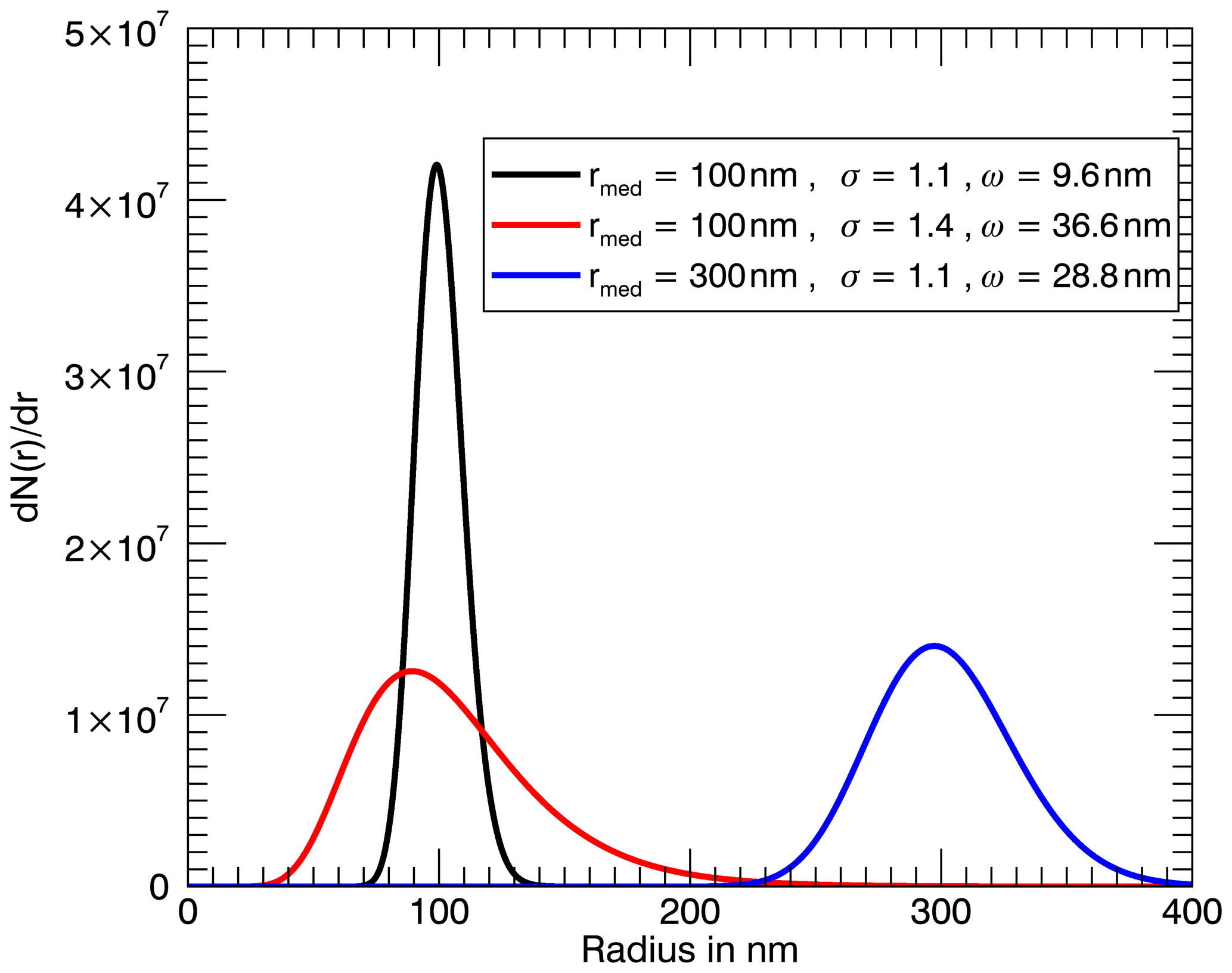
Figure 3 Three exemplary monomodal log-normal size distributions with different combinations of the median radius and distribution width σ. Additionally, the absolute distribution width ω is given. This figure illustrates that ω is more closely related to the width of the PSD in linear radius space, i.e., the radius range covered by the distribution, than σ.

4.1 Ambae eruptions, 2017–2018

In Fig. 4, the effects of the Ambae eruptions on the stratospheric aerosol layer can be seen.

In the first row of plots the closest to background conditions before the two main eruptive phases in April and July 2018 are shown, namely monthly averages for March. Nevertheless, the number density and the extinction coefficient are already enhanced. For the Northern Hemisphere this can be attributed primarily to the Canadian wildfires of 2017, which was the burning season with the largest area burned in British Columbia since beginning of the recording (Ansmann et al., 2018). However, there is also a signal in the Southern Hemisphere with enhanced number densities and extinction coefficients and low median radius values. This signal first showed up in the Southern Hemisphere in October 2017 (not shown). This is more of a mystery but could be a consequence of several smaller tropical volcanic eruptions in late 2017, which, to our knowledge, did not directly inject SO₂ above the tropopause. These include the Tinakula (10.4^∘ S) eruption on 21 October, whose ash and gas plume reached up to 10.7 km altitude (Laiolo et al., 2018); the Agung (10.4^∘ S) eruption on 21 November, with an ash plume reaching 9.1 km (Global Volcanism Program, 2023); and Ambae's (15^∘ S) first two, less explosive eruptive phases, which lasted from 22 September to 6 October 2017 and from 21 October to 7 December 2017 (Moussalam et al., 2019). Since these are all tropical volcanoes, it is conceivable that some of the sulfur precursor gases emitted could have been transported into the lower stratosphere across the tropical tropopause layer (TTL) (Kremser et al., 2016).

The second row of plots in Fig. 4 depicts the month of June. Here, the effects of the third eruptive phase can be seen, which lasted from mid-March to mid-April 2018. This third eruptive phase was explosive enough to inject SO₂ directly into the lower stratosphere, with the largest injection period occurring on 6 April. In the third row, which shows monthly means for September 2018, the impacts of the fourth and most active eruptive period of Ambae in July are visible. In July the largest amount of SO₂ was emitted, with 0.35–0.4 Tg SO₂ (Global Volcanism Program, 2023).

The extinction coefficient and the number density both show a distinct enhanced layer in the lowermost stratosphere above the tropopause that stands out from the much lower values at higher altitudes, where the signals of the Canadian wildfires and the unknown perturbation in the Southern Hemisphere in 2017 still relax more towards background conditions. This enhanced layer can be seen in June after the third eruptive phase, but it becomes much stronger after the July eruptions. As described before, both hemispheres are affected by the eruptions (Malinina et al., 2021).

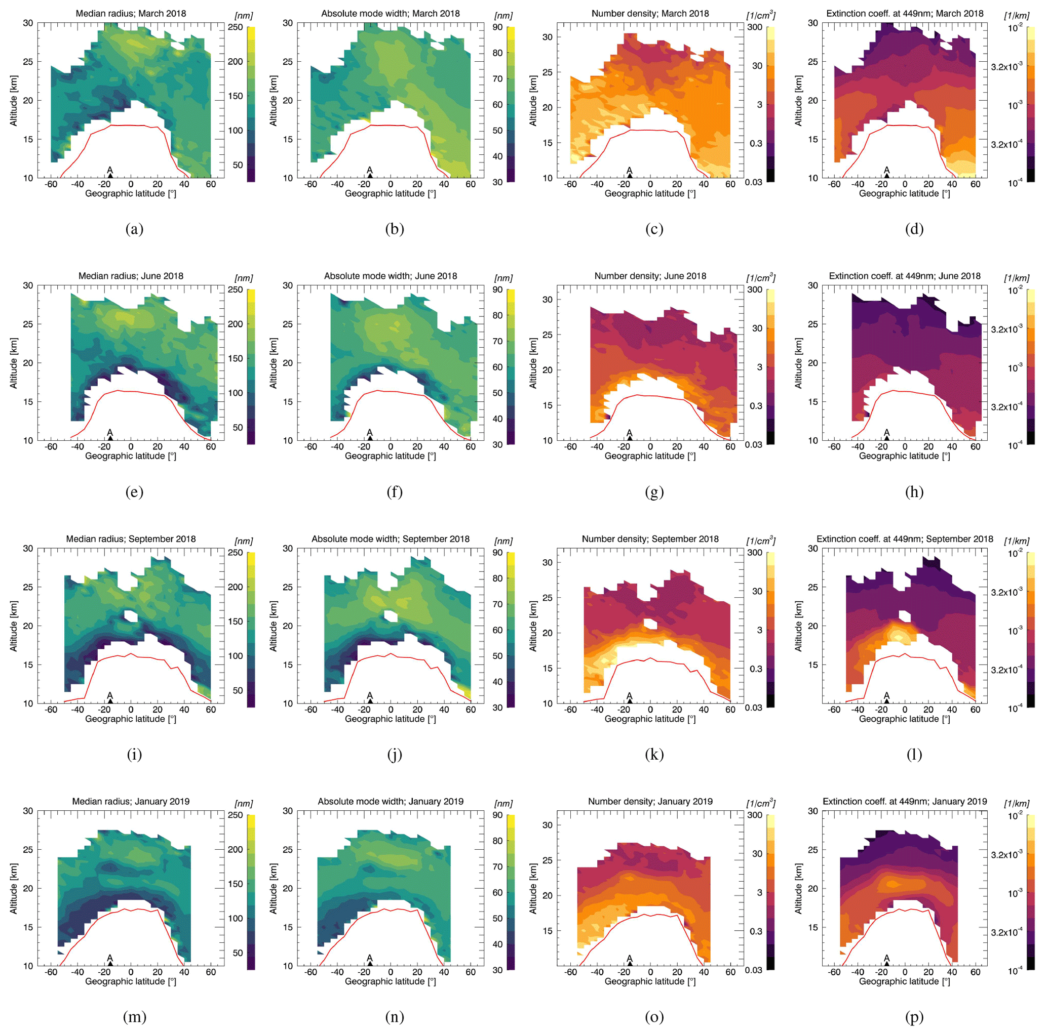
Figure 4 Median radius (leftmost column), absolute distribution width ω (second column), number density (third column) and extinction coefficient at 449 nm (rightmost column) for characteristic months before and after the Ambae eruptions in 2018. The location of the volcano is marked with a triangle and letter on the bottom of each plot, and tropopause height is indicated by a red line.

The most notable and surprising signal, though, is the strong decrease in the median radius and absolute distribution width in that same enhanced layer above the tropopause, mostly below 20 km altitude. This means that the particle size distribution (PSD) shifts towards smaller aerosol radii, while also becoming more narrow. Therefore the Ambae eruptions seem to have led to a domination of a large number of smaller aerosol droplets in the lowermost stratosphere. It is also remarkable that the PSD stays in this configuration of on average very small aerosol particles for many months, as in January the signal is still very clear, although already diminished. These findings will be discussed more in depth in Sect. 5. Over time, an interesting layering emerges in the tropics that is best visible in January 2019 (lowermost row), where a layer of larger values of the median radius and absolute distribution width resides at roughly 21 km altitude with very small average aerosol sizes above and below.

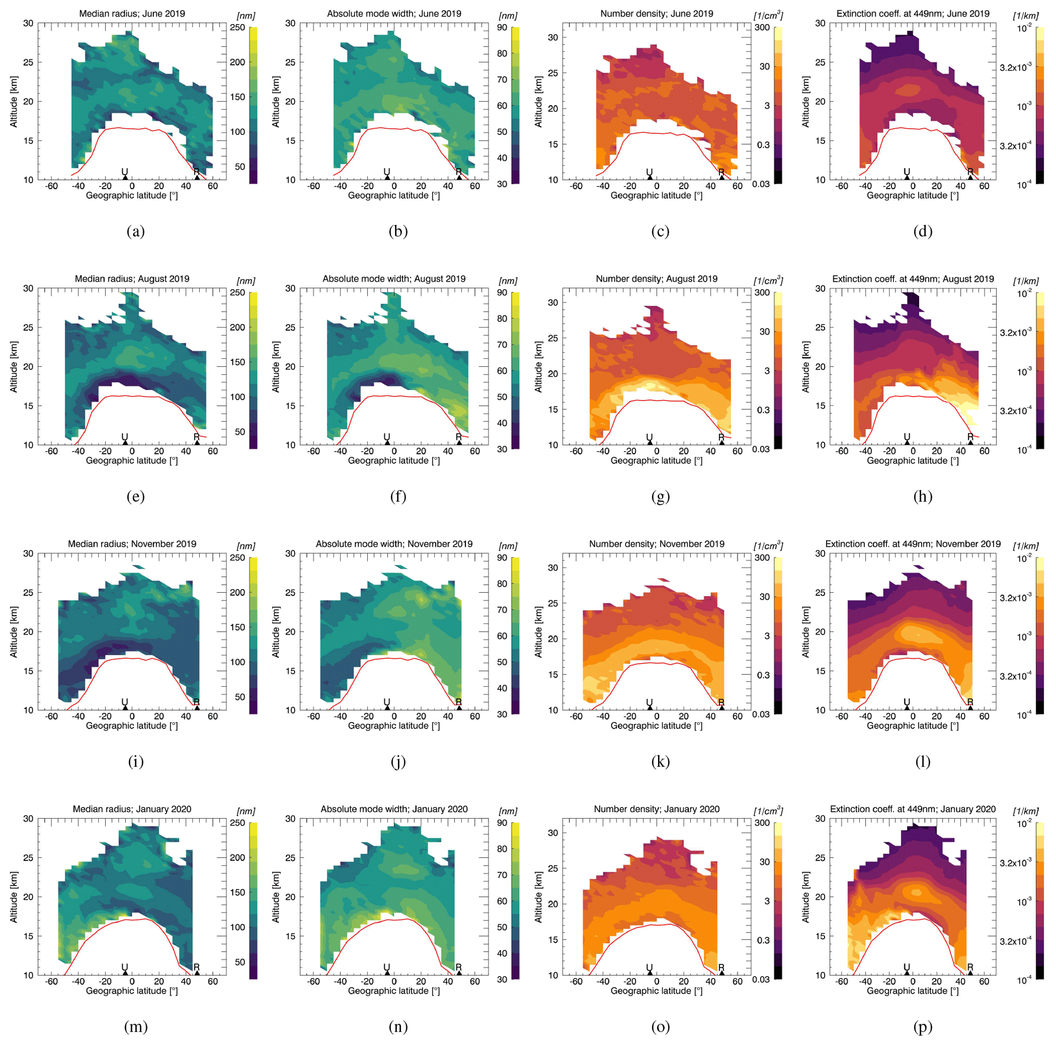
4.2 Raikoke and Ulawun eruptions, 2019

In Fig. 5 the PSD parameter evolution for the eruptions of Raikoke and Ulawun in the summer of 2019 are depicted. In the first row, an average over the time between 1 to 20 June is shown, i.e., before the Raikoke and Ulawun eruptions on 22 and 26 June, respectively. This is the closest to background conditions before this phase of volcanic activity. At this point, the effects of the Ambae eruptions in the year before have diminished strongly, although the extinction coefficient is still slightly enhanced throughout the main Junge layer.

In August, after the June eruptions of Raikoke and Ulawun and after the second Ulawun eruption on 3 August, an increase in the extinction coefficient over both the Northern and Southern Hemisphere occurred, as expected. The signal is much stronger in the Northern Hemisphere, since the Raikoke eruption emitted more SO₂ (around 1.37 Tg) than both Ulawun eruptions together (around 0.44 Tg combined).

However, regarding the PSD parameters a unique pattern emerges, where Ulawun and Raikoke had opposite effects. Over the broad Raikoke area and in the lowermost stratosphere below roughly 15 km, the median radius, absolute distribution width and number density increase from June to August. In contrast, in the Southern Hemisphere values of the median radius and absolute distribution width show a strong decrease. This goes along with an especially strong increase in the number density in the Southern Hemisphere. This means that the Southern Hemisphere is dominated by a high number of very small aerosol particles below roughly 20 km, which notably stay small until the end of the year, similar to the effects of the Ambae eruptions in the previous year. The average aerosol size stays small at least until November 2019. In January 2020 the signal is covered by emissions stemming from the Australian wildfires of 2019–2020, which were unprecedented in the destruction caused and in the area affected by high-severity fire (Collins et al., 2021). The PSD parameters affected by these wildfires in the last row of plots are not reliable though, since the assumptions on the shape of the size distribution as well as on the refractive indices of the aerosol made in the retrieval of this work may not be realistic for these conditions.

Although the Raikoke eruption emitted around 15 Tg of ash (Osborne et al., 2022), it was only detectable in the atmosphere for a few days and roughly 90 % of it was removed from the atmosphere within 48 h (Prata et al., 2022). Therefore, it is unlikely to play a big role in the retrieval data presented in Fig. 5. Nevertheless, the signals visible in the Northern Hemisphere may not be attributable to the Raikoke eruption alone, since there also have been two different severe wildfire events in the Northern Hemisphere in 2019 that were strong enough to reach the stratosphere (Voronova et al., 2020; Osborne et al., 2022). It is still not clear if and to what extent there was interaction between smoke and the sulfate aerosol plume originating from the Raikoke eruption. Therefore it cannot be excluded that smoke might have played a role in the aerosol size increase retrieved in the volcanic period displayed in the Northern Hemisphere.

Figure 5 Analogous to Fig. 4 but for the months around the Raikoke and Ulawun eruptions.

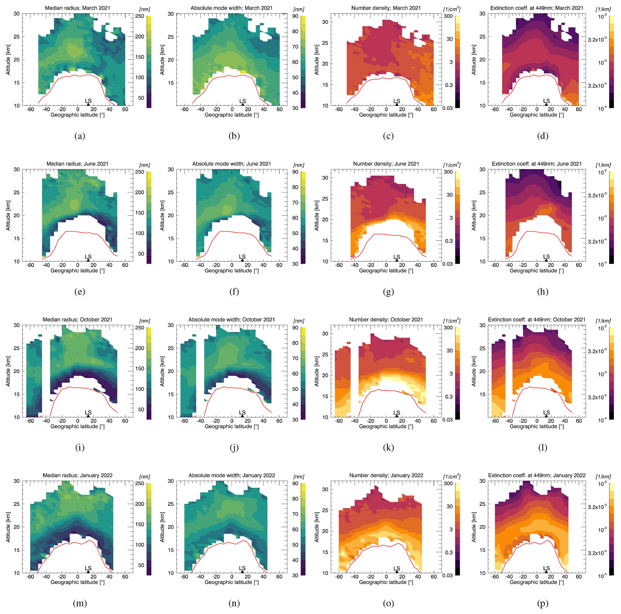
4.3 La Soufrière eruption, 2021

In Fig. 6, the period of volcanic activity before and after the La Soufrière eruptions between 9–22 April 2021 is depicted.

The first explosive eruptions happened on 9 April throughout the day with the ash plume reaching up to 8 km. Explosive activity on 10 and 11 April led to ash plumes rising up to 16 km in altitude. In the following days more volcanic activity was observed, although plume heights did not exceed 12 km anymore (Yue et al., 2022; Bruckert et al., 2023). Based on TROPOMI measurements, La Soufrière emitted roughly 0.4 Tg of SO₂.

The patterns in the PSD parameters as well as in the extinction coefficient that emerge are very similar to those observed for the period of the Ambae eruptions in 2018 (Fig. 4). The aerosol cloud spreads over both hemispheres, visible in an increase in the number density and extinction coefficient in the lowermost stratosphere slowly affecting higher altitudes over time. Notably, there again is a strong decrease in median radii and absolute distribution widths after the La Soufrière eruptions in both hemispheres in the same altitude region. Both parameters stay very low due to the eruptions at least until January 2022. A slow rising of the enhanced aerosol layer in the tropics from around 20 km altitude in June 2021 up to around 23 km in November 2021 can be observed in all PSD parameters. On 15 January the Hunga Tonga–Hunga Ha'apai eruption happened, which was very unusual in many ways and introduced perturbations into the stratosphere which are not shown or discussed here (Legras et al., 2022).

Figure 6 Analogous to Fig. 4 but for the months around the La Soufrière eruption.

5 Discussion of the SAGE III/ISS retrieval results

This satellite observation of the size reduction in the aftermath of the Ambae, Ulawun and La Soufrière eruptions is unprecedented. While there is some evidence in previously published literature that some volcanic eruptions lead to changes in extinction ratios at two wavelengths (Rieger et al., 2014; Thomason et al., 2021), this cannot easily be interpreted as an increase or decrease in aerosol size, as will be shown below. Indeed, this kind of analysis using two wavelengths can be helpful to detect differences in the effect of volcanic eruptions on the aerosol size in the first place, but the amount of concrete information on the particle size distribution itself is inherently limited, since with only two pieces of independent spectral information the distribution width σ is usually fixed at an assumed value in order to retrieve the median radius. This is a large source of error, since the retrieval carried out in this work using the SAGE III/ISS data set strongly suggests that the distribution width of a monomodal log-normal size distribution of stratospheric aerosol varies in time and space. As Malinina et al. (2019) pointed out, there are a lot of different possible combinations of the median radius and distribution width values that would lead to the same extinction ratio at two wavelengths.

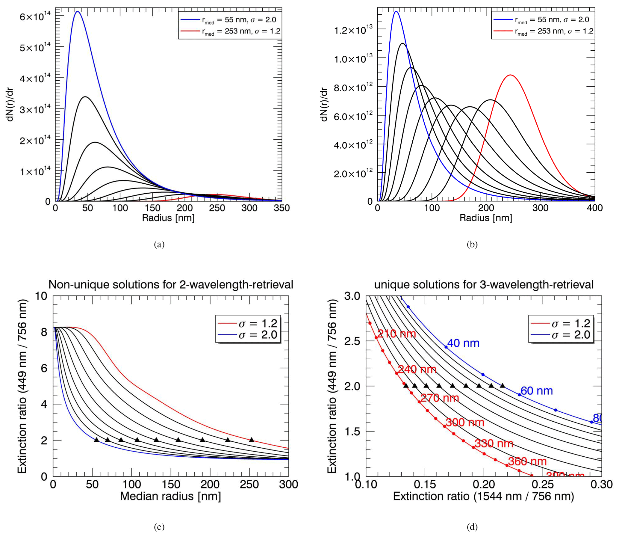
Figure 7 Panel (a) shows nine different monomodal log-normal size distributions that are all valid solutions for an exemplary extinction ratio of 2 at the wavelengths 449 nm : 756 nm. The individual curves with different median radii and number densities result from a different assumption on the distribution width σ (in steps of 0.1 between 1.2 and 2.0), which is necessary when only two wavelengths are used. For visual clarity (b) shows the same PSDs as (a) but with their number densities scaled to the same value. Panel (c) shows the lookup table used to retrieve the median radii of the PSDs in (a) and (b), using two wavelengths, with which the true size distribution cannot be identified. Triangles indicate the different non-unique solutions. Panel (d) shows a lookup table using three wavelengths and two extinction ratios, for which unique solutions exist, since each triangle corresponds to a different value of the second extinction ratio.

This is illustrated in Fig. 7a, where nine different calculated monomodal log-normal size distributions are shown that are all consistent with the same exemplary extinction ratio of 2.0 for the wavelengths 449 nm : 756 nm, which in this case functions as hypothetical measurement data. Since only two wavelengths are used, the distribution width has to be assumed. Each of the depicted PSDs is based on the retrieval of the median radius assuming a different distribution width between 1.2 and 2.0 in steps of 0.1 using the extinction ratio of 2.0 with a standard two-wavelength retrieval method. After the retrieval of the median radius the number density was calculated. The PSD plotted in blue is the result for the maximum assumed distribution width of 2.0, which resulted in a median radius of 55 nm (corresponding to an effective radius of 183 nm); the red curve corresponds to the smallest assumed σ of 1.2 with a retrieved median radius of 253 nm (effective radius of 275 nm). All depicted PSDs, including the red and blue curves, represent possible solutions if the aerosol size retrieval was performed using only two wavelengths. These solutions are very different, and we would not know which one is closest to the truth; therefore we could not conclude in which way the size distribution of the stratospheric aerosol changes after volcanic eruptions when using only two wavelengths. To emphasize this, note that the median radius values in this example almost span the range of the median radius variability observed in the SAGE III/ISS retrieval data of this work. Fig. 7b shows the same PSDs as Fig. 7a, but each distribution is scaled to the same number density to help visual distinction of the different curves. In Fig. 7c, the curves of the lookup table that was used to retrieve the median radii of the PSDs in Fig. 7a are depicted. For each curve extinction ratios at the wavelengths 449 nm : 756 nm were calculated using Mie theory for a range of median radius values. Each curve corresponds to a single σ value between 1.2 and 2.0. A different median radius value will be retrieved depending on the assumption of the distribution width (i.e., no unique solution exists), as illustrated by the triangles marking the position of the exemplary extinction ratio of 2.0. In contrast, using the second lookup table shown in Fig. 7d (similar to what was used in this work), the distribution width σ can be retrieved along with the median radius, since, here, two extinction ratios using three wavelengths are used. These curves are calculated in the same way as the ones of Fig. 7b, except that a third wavelength – in this case 1544 nm – is included. If such a lookup table is used, the triangles, although still marking the extinction ratio at 449 nm : 756 nm of 2.0, do not mark equally valid solutions for the particle size retrieval. Instead, due to the second extinction ratio, the distribution width can be retrieved along with the median radius and does not have to be assumed anymore. This way, a unique solution emerges for both parameters, and the ambiguity illustrated by the large differences between the size distributions of Fig. 7a is eliminated.

This is where the observational data set presented in this work can contribute to our understanding of how the stratospheric aerosol size changes after volcanic eruptions. Since the retrieval method is based on three wavelengths (Wrana et al., 2021), much more information on the actual shape of the size distribution is gained, still under the assumption of a monomodal log-normal PSD.

While the small sample size of volcanic eruptions investigated in this work makes it difficult to draw generalized conclusions, the volcanic eruptions of Ambae in 2018, Ulawun in 2019 and La Soufrière in 2021 which produced the strong reduction in average stratospheric aerosol size share some similarities. They emitted similar amounts of SO₂, i.e., close to 0.4 Tg. In contrast, Raikoke, whose eruption in 2019 did not lead to an observed size decrease but instead to an increase, emitted around 1.37 Tg SO₂. In addition, the former three volcanoes are all tropical, whereas Raikoke is situated in northern middle latitudes, at around 48^∘ N. This could be important insofar as, depending on the season, there are temperature differences in the lowermost stratosphere between low and middle latitudes. Temperature is an important factor in nucleation and condensation rates, which are integral lifetime processes of stratospheric aerosol and play an important role in their size evolution (Kremser et al., 2016). Nucleation strongly increases with decreasing temperatures (Vehkamäki et al., 2002; Korhonen et al., 2003), which can shift the sulfate aerosol size distribution towards smaller sizes (Pirjola et al., 1999).

The assumption that the true size distribution of stratospheric aerosol can be described well by a monomodal log-normal size distribution is at the core of the observational data presented here. This assumption is made frequently for satellite retrieval data sets, not only because it is a reasonable assumption for many cases but also because it is often necessary to limit the number of unknown variables of the PSD in order to still be able to solve for them using the limited amount of independent information contained within a measurement. Indeed, in some cases the truth is probably closer to a bimodal log-normal distribution (Deshler et al., 2003). However, the false assumption of a monomodal log-normal size distribution in a bimodal log-normal case would lead to an overestimation of the particle size in a satellite occultation measurement data set like the SAGE III/ISS data used in this work (von Savigny and Hoffmann, 2020). This is because the second mode, although containing far fewer aerosol particles, would contain larger aerosol particles which, in the size regime typical of stratospheric aerosol, are much more efficient scatterers and would dominate the spectral signal picked up by the instrument. In turn, a retrieval based on the assumption of a monomodal log-normal size distribution would produce a PSD shifted towards larger radii. Therefore, the signal of a size distribution shifted towards very small radii, which is observed in the volcanic periods discussed in this study, cannot be the result of a wrong assumption on the size distribution shape.

6 Comparison: model vs. observations

In order to learn whether current models, in this case the ECHAM model, can help us to identify and understand the main dynamical and microphysical factors controlling the aerosol size evolution after volcanic eruptions, specifically the observed particle size reduction, model simulations of the time period before and after the Raikoke and Ulawun eruptions in 2019 were carried out. This period of volcanic activity was chosen because here an average aerosol size reduction is found in the Southern Hemisphere and tropics (over Ulawun) alongside an average aerosol size increase in the Northern Hemisphere (over Raikoke) at the same time. This makes it a useful case to test whether the model can reproduce the differences in aerosol size evolution after these eruptions in order for it to be used to gain a better understanding of the related processes.

6.1 Simulation of Raikoke and Ulawun, 2019

In the simulations, SO₂ masses that are vertically resolved in three altitude levels are injected into the lower stratosphere at the locations of the Raikoke and Ulawun volcano at the time of each of the eruptions. Consequently, the evolution of the particle size distribution of the forming sulfate aerosol is calculated. Multiple model runs were performed with varying input parameters. The relevant parameters used for the best model run, which is used in this work, are shown in Table 2. The SO₂ mass injected into the stratosphere for the second eruption of Ulawun is taken from Kloss et al. (2021), and parameters for the other two eruptions come from our own SO₂ mass estimation using the TROPOMI data set. Like in the SAGE III/ISS retrieval the stratospheric aerosol is assumed to be composed of sulfuric acid and water only. In order to start the Raikoke and Ulawun simulations with background conditions comparable to the observations, the simulation is started from a 10-year simulation on 1 January 2018. By doing that, the Ambae eruptions are included in the run. If the Ambae eruptions were not included, the simulated atmosphere would end up too “clean” in June 2019, before the Raikoke and Ulawun eruptions, and therefore not be comparable to observations.

Table 2 Relevant parameters of the Raikoke and Ulawun eruptions as used in the ECHAM simulations.

In the model simulations ash is included, but there is no interaction with the sulfate aerosol; i.e., no mixed ash–sulfate aerosol is calculated. Regarding the aerosol particle size, ECHAM uses a modal model. Four log-normal distributions are considered, which are called, sorted from smaller to larger radii, the nucleation mode, Aitken mode, accumulation mode and coarse mode. Each of these modes has a fixed distribution width σ and a median radius that can change within certain value ranges. The number densities within the individual modes change as well, as a result of the calculated microphysical processes like the nucleation, condensation and coagulation rates.

6.2 Extinction

Here, the extinction coefficient at 550 nm is compared between the observational SAGE III/ISS data and the ECHAM simulations. In the SAGE III/ISS solar occultation level 2 data set the extinction coefficient is not provided at 550 nm directly. To address this, a third-order polynomial was fitted to the extinction spectra using the six most reliable wavelength channels of the data set, i.e., 449, 521, 756, 869, 1021 and 1544 nm, to retrieve extinction coefficients at 550 nm that can then be used for comparison.

In Fig. 8, zonal averages of the extinction coefficient at 550 nm are depicted for the time before the volcanic eruptions (left column), i.e., between 1 and 20 June 2019, and for August of 2019 (right column). The panels in the upper row show the data that were calculated from the SAGE III/ISS measurements, while the panels in the lower row depict results from the ECHAM simulations. As explained in Sect. 2, the spatial and temporal sampling of SAGE III/ISS is limited. Therefore, to acquire actually comparable temporal and spatial coverage between the observational and model data set, we applied the sampling of the SAGE III/ISS measurements to the model output. In other words, only profiles from the ECHAM simulations for locations and times were included, where SAGE III/ISS measurements happened on the same day within 1^∘ of longitude and 2.5^∘ of latitude. As in Sect. 4 this means that data in different latitude bins correspond to different days within the month depicted. The tropopause height shown was provided in the SAGE III/ISS level 2 data set, taken from the MERRA-2 (Modern-Era Retrospective analysis for Research and Applications) reanalysis data. The blue line marks a 1 km interval above this calculated tropopause height, above which it is unlikely that the measurements are affected by clouds or include tropospheric air in general.

The background conditions in prevolcanic June 2019 are reproduced very well by the ECHAM simulations, both in magnitude of the values and in the spatial patterns emerging, aside from an enhanced extinction between 40^∘ N and 60^∘ N below 14 km in the SAGE III/ISS data. This perturbation may be smoke from the two larger wildfires that reached the lowermost stratosphere, which is not included in the model. For August 2019, in general the ECHAM simulations could reproduce the observations as well, although in the SAGE III/ISS data the perturbations of the extinction coefficient partly reach higher altitudes in the northern latitudes. Both the model and observations show a strong increase in the extinction, with a much stronger effect over the latitudes near Raikoke.

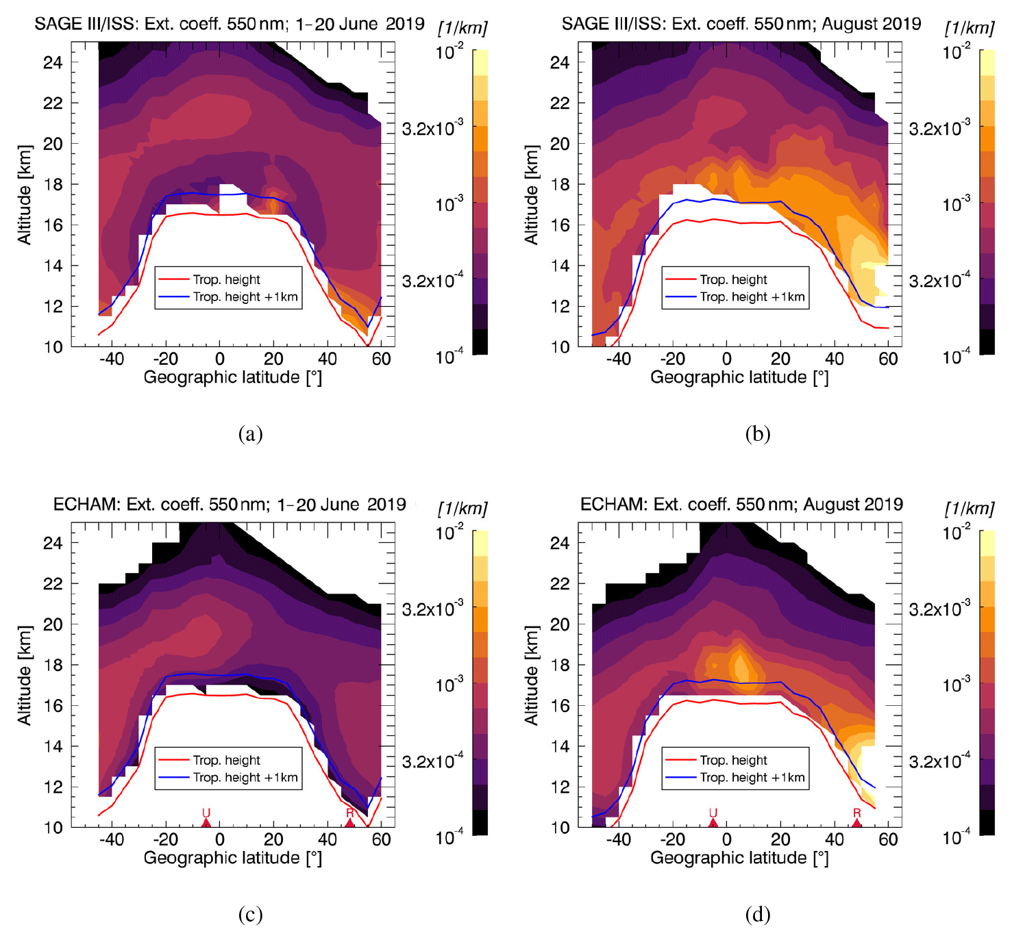
Figure 8 Zonal means of the aerosol extinction coefficient at 550 nm for (a, c) 1 to 20 June and (b, d) August 2019 from the (a, b) SAGE III/ISS data set and from the (c, d) ECHAM simulations using the spatial and temporal sampling of SAGE III/ISS. Triangles and letters on the bottom of each plot indicate the locations of the Ulawun (U) and Raikoke (R) volcano. Tropopause height is illustrated by a red line, with the blue line indicating an uncertainty interval of 1 km above the tropopause height.

6.3 Effective radius

The effective radius is the area-weighted mean radius of the size distribution (Grainger, 2017). It is a useful quantity since with it a particle size distribution can be expressed using only one parameter. Furthermore, it can be used to compare PSDs of different shapes. This is necessary in this case, since our SAGE III/ISS retrieval data set includes monomodal log-normal size distribution, while in the ECHAM model output, the PSD is expressed in terms of four individual log-normal modes. The effective radius r_eff from the ECHAM simulations, representing these four modes, is calculated in the following way:

$$\begin{array}{}\text{(4)}& r_{\mathrm{eff}}={\displaystyle \frac{\int r^{\mathrm{3}}n\left(r\right)\mathrm{d}r}{\int r^{\mathrm{2}}n\left(r\right)\mathrm{d}r}}={\displaystyle \frac{m_{\mathrm{3}}}{m_{\mathrm{2}}}},\end{array}$$

where m₃ is the third moment and m₂ is the second moment of the particle size distribution.

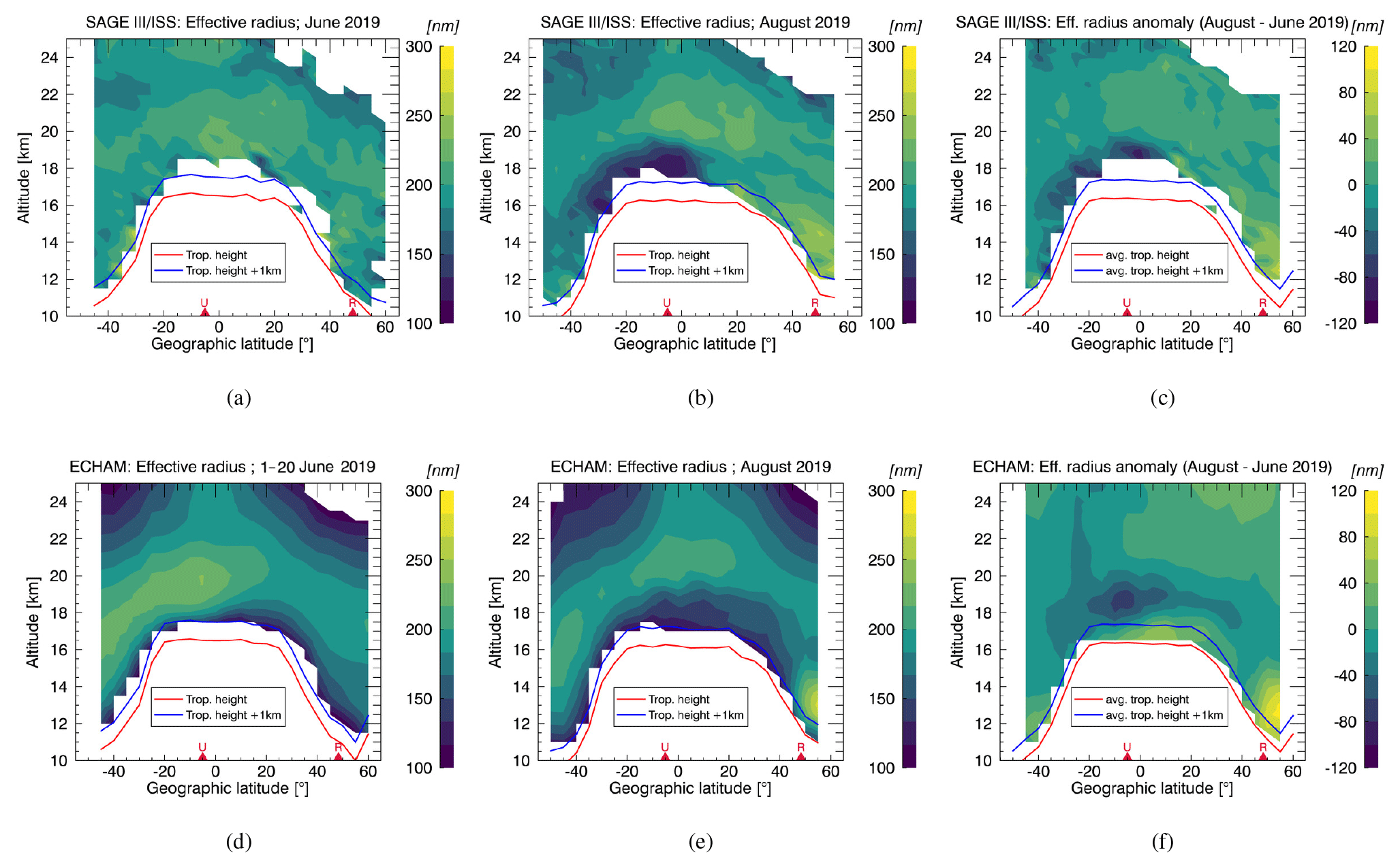
Figure 9 Zonal means of the effective radius (a–c) retrieved from SAGE III/ISS and (d–f) calculated with the ECHAM model using the spatial and temporal sampling of SAGE III/ISS for (a, d) 1 to 20 June and (b, e) August 2019. Panels (c) and (f) show the temporal anomaly of the effective radius, i.e., the difference between the first two plots in each row. Triangles and letters on the bottom of each plot indicate the locations of the Ulawun (U) and Raikoke (R) volcano. Tropopause height is illustrated by a red line, with the blue line indicating an uncertainty interval of 1 km above the tropopause height.

The effective radii retrieved from the SAGE III/ISS observations in Fig. 9a and b show an increase over the Raikoke area from June to August 2019 in the lowermost stratosphere roughly between 40 and 60^∘ N. Most notably, there is a large reduction in the effective-radius values over the Ulawun area (around 5^∘ N to 35^∘ S) over the same time span, analogous to the reduction in the median radius and absolute distribution width that was discussed before in Sect. 5. This reduction in average particle size persists at least until November 2019 (see Appendix). In Fig. 9c, the effective-radius temporal anomaly, i.e., the difference between Fig. 9b and a, is depicted, which makes it clear where the effective radius increased and where it decreased from June to August. Over the Raikoke area an increase in the effective radius by up to 87 nm is found, and in the tropics and southern subtropics there is a decrease by up to 123 nm. It has to be noted that part of the Raikoke plume has been missed because of the limited spatial coverage of the SAGE III/ISS measurements, since a substantial part of the plume was transported further north than 60^∘ N (Kloss et al., 2021).

The lower row of panels in Fig. 9 is analogous to the upper row but shows the ECHAM simulations for the same time frames. For the background conditions (Fig. 9d) effective radii in the lowermost kilometer above the tropopause are much lower than in the SAGE III/ISS retrieval data. Apart from this effective radii are close to the observations. In August, the qualitative pattern of high values in the lowermost stratosphere over Raikoke and low values over the broad Ulawun region is reproduced by the model. Also in Fig. 9f, which again shows the temporal anomaly, the absolute increases and decreases in the regions affected by the volcanic eruptions mostly match the observations well. The effective-radius increase over the Raikoke area in the lowermost stratosphere is stronger in the model, which is because of the low effective radii in this region in the model's background. The smaller effective radii in Fig. 9e and the region of decrease in Fig. 9f reach further into the Northern Hemisphere than in the observations.

Starting in September 2019, the model and observations start to diverge: effective radii stay very low over the tropics and southern subtropics in the SAGE III/ISS retrieval data until December of 2019, before the Australian wildfires cover the signal in January 2020. In contrast, the model calculates strong particle growth in the months after August, with effective radii increasing far beyond the background at higher altitudes. This suggests that the MAECHAM5-HAM model can be used to learn about the stratospheric aerosol evolution and its underlying mechanisms in the short term after volcanic eruptions. In the longer term, however, the comparison reveals differences which may point towards the microphysical evolution in the model. Identifying the cause of this discrepancy between the model and observations is difficult. Possible causes could in principal be an overestimation of coagulation by the model, a lack of interactive OH chemistry in the model, deviations in dynamics (e.g., due to smaller vertical advection in ECHAM compared to other models; Niemeier et al., 2020), or biases in the observational data set or the retrieval algorithm. To investigate this, comparisons with different models need to be conducted.

7 Conclusions

Using a multi-wavelength extinction ratio approach we retrieved particle size distribution parameters of stratospheric aerosol from the SAGE III/ISS satellite solar occultation data set. As a result of the assumption of a monomodal log-normal size distribution, we retrieved the median radius, distribution width and total number density, as well as the absolute distribution width and effective radius for understandability and comparison purposes.

We looked at the temporal evolution of these parameters in three different periods of volcanic activity in the SAGE III/ISS data set, the first one being associated with the eruptions of Ambae in 2018, the second one being associated with the Raikoke and Ulawun eruptions in 2019, and the third one being associated with the La Soufrière eruption of 2021. Surprisingly, we found that the average aerosol size decreased for all of the mentioned eruptions, except for the Raikoke eruption. This is very different from, e.g., the Mt. Pinatubo eruption of 1991, which is probably the volcanic eruption on which the most research was done in total, where aerosol size increased (Deshler et al., 2003). For the Ambae, Ulawun and La Soufrière eruptions instead, the median radius, absolute distribution width and effective radius decreased strongly; i.e., the PSD became narrower and shifted towards smaller radii. We also showed that, for this finding, the use of a three-wavelength extinction approach to retrieving stratospheric aerosol size as opposed to a standard two-wavelength extinction approach was crucial. This way, the distribution width did not have to be assumed, and the strong ambiguity inherent to two-wavelength retrievals is removed. Notably, this strong reduction in average aerosol size also lasted for months in each case and even over a year in La Soufrière's case, when the perturbed aerosol layer could evolve more or less undisturbed.

In order to better understand the importance of different microphysical and dynamical processes at play in the size decrease as well as in the long lifetime of the very small average aerosol sizes, atmospheric models will be a necessary and important tool of investigation. Because of this we performed simulations of the Raikoke and Ulawun volcanic activity period in 2019 with the aerosol climate model MAECHAM5-HAM. To compare the monomodal log-normal size distributions of our SAGE III/ISS retrieval data with the four-mode log-normal PSD of the ECHAM model, the effective radius was used. The model was able to reproduce well the spatial and temporal patterns that were observed in the SAGE III/ISS data in the extinction coefficient at 550 nm and the effective radius from June to August 2019, i.e., the decrease in average stratospheric aerosol size over Ulawun and the increase over Raikoke. In this study we found it to be essential to include preceding large injections of sulfur-containing gases into the stratosphere, in this case the eruptions of the Ambae volcano in 2018, since without them the simulated atmosphere would be too clean in the background conditions before Raikoke and Ulawun compared to observations. Despite this encouraging agreement with the SAGE III/ISS retrieval data in the first 2 months, there is a growing discrepancy between the model and observations in the months thereafter. In other words, the model could not reproduce the long lifetime of the small aerosol size, and instead the effective radii strongly increased in the simulations after the initial PSD parameter reduction over Ulawun.

Further research is needed, especially on the conditions necessary for a stratospheric aerosol average size decrease after volcanic eruptions to occur as opposed to a size increase. This may be an important pathway to improve the capability of climate models to reproduce observed effects of volcanism on climate and reduce uncertainty in simulations when including volcanic eruptions. For this we will need more intercomparisons between observational data and model simulations in terms of stratospheric aerosol size.

Appendix A: Other quantities related to aerosol size

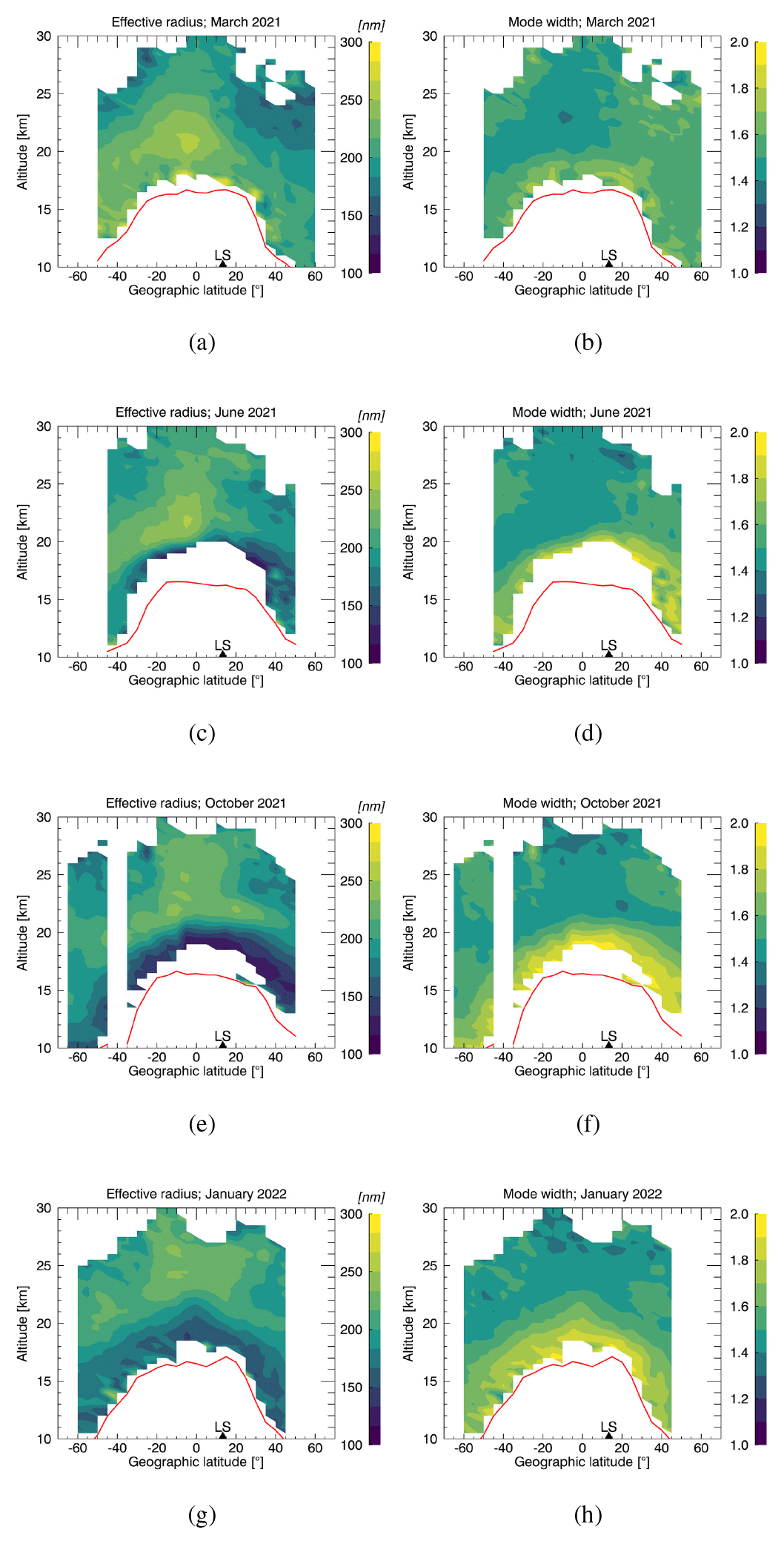
Here, we provide two additional quantities related to the stratospheric aerosol size distributions retrieved from the SAGE III/ISS data set for the three main volcanic periods covered in Figs. 4 to 6. The two quantities are the effective radius, which is explained in Sect. 6.3, and the distribution width σ or geometric standard deviation, which is part of Eq. (1).

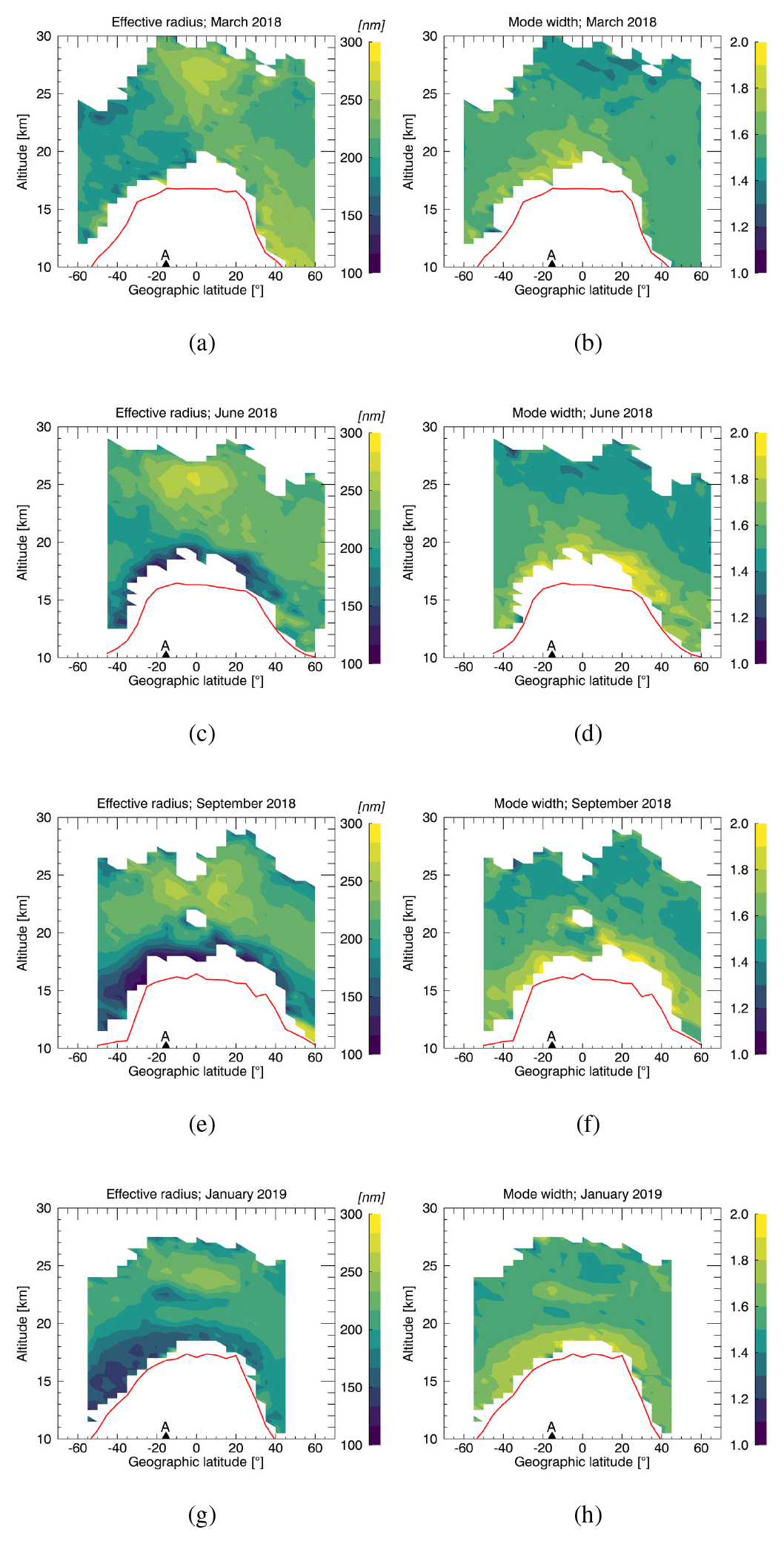
Figure A1 Analogous to Fig. 4 but showing the effective radius and the distribution width σ for the characteristic months before and after the Ambae eruptions in 2018.

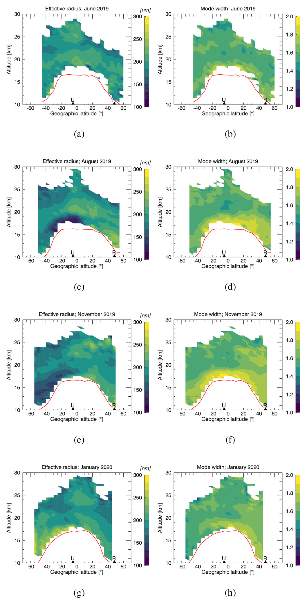
Figure A2 Analogous to Fig. A1 but for the characteristic months before and after the Raikoke and Ulawun eruptions in 2019.

Figure A3 Analogous to Fig. A1 but for the characteristic months before and after the La Soufrière eruption in 2021.