the Creative Commons Attribution 4.0 License.
the Creative Commons Attribution 4.0 License.
 | 24 Aug 2023
Explaining apparent particle shrinkage related to new particle formation events in western Saudi Arabia does not require evaporation
Ville Vakkari
Heikki Lihavainen
Antti-Pekka Hyvärinen
Kimmo Neitola
Jenni Kontkanen
Veli-Matti Kerminen
Markku Kulmala
Tuukka Petäjä
Tareq Hussein
Mamdouh I. Khoder
Mansour A. Alghamdi
Pauli Paasonen
The majority of new particle formation (NPF) events observed in Hada Al Sham, western Saudi Arabia, during 2013–2015 showed an unusual progression where the diameter of a newly formed particle mode clearly started to decrease after the growth phase. Many previous studies refer to this phenomenon as aerosol shrinkage. We will opt to use the term decreasing mode diameter (DMD) event, as shrinkage bears the connotation of reduction in the sizes of individual particles, which does not have to be the case. While several previous studies speculate that ambient DMD events are caused by evaporation of semivolatile species, no concrete evidence has been provided, partly due to the rarity of the DMD events. The frequent occurrence and large number of DMD events in our observations allow us to perform statistically significant comparisons between the DMD and the typical NPF events that undergo continuous growth. In our analysis, we find no clear connection between DMD events and factors that might trigger particle evaporation at the measurement site. Instead, examination of air mass source areas and the horizontal distribution of anthropogenic emissions in the study region leads us to believe that the observed DMD events could be caused by advection of smaller, less-grown particles to the measurement site after the more-grown ones. Using a Lagrangian single-particle growth model, we confirm that the observed particle size development, including the DMD events, can be reproduced by non-volatile condensation and thus without evaporation. In fact, when considering increasing contributions from a semivolatile compound, we find deteriorating agreement between the measurements and the model. Based on these results, it seems unlikely that evaporation of semivolatile compounds would play a significant role in the DMD events at our measurement site. In the proposed non-volatile explanation, the DMD events are a result of the observed particles having spent an increasing fraction of their lifetime in a lower-growth environment, mainly enabled by the lower precursor vapor concentrations further away from the measurement site combined with decreasing photochemical production of condensable vapors in the afternoon. Correct identification of the cause of the DMD events is important as the fate and the climate relevance of the newly formed particles heavily depend on it – if the particles evaporated, their net contribution to larger and climatically active particle sizes would be greatly reduced. Our findings highlight the importance of considering transport-related effects in NPF event analysis, which is an often overlooked factor in such studies.
- Article
(10401 KB) - Full-text XML
- BibTeX
- EndNote


The largest uncertainty in our ability to quantify present-day climate change is related to the role of atmospheric aerosols (IPCC, 2021). The climate impact of aerosol particles mainly stems from aerosol–cloud interactions. Thus, particles large enough (diameter Dp > 50–100 nm) to act as cloud condensation nuclei (CCN) are of specific interest. In the atmosphere, the majority of CCN form via the growth of sub-CCN-sized aerosol particles that originate from either atmospheric new particle formation (NPF), in which new particles are formed from vapor molecules, or emissions of small primary particles (Merikanto et al., 2009; Kerminen et al., 2012; Paasonen et al., 2013; Gordon et al., 2017; Liu and Matsui, 2022). Therefore, the growth of small particles plays an essential role in aerosol–climate interactions, but the dynamics causing the particle growth and the chemical compounds involved are not yet adequately quantified (Zhang et al., 2012; Tröstl et al., 2016; Paasonen et al., 2018; Semeniuk and Dastoor, 2018).
In general, the most important driver of small particle growth up to CCN sizes is considered to be the condensation of low-volatility oxidation products of volatile organic compounds (VOCs) (Smith et al., 2008; Laaksonen et al., 2008; Jimenez et al., 2009; Riipinen et al., 2012; Ehn et al., 2014; Kerminen et al., 2018; Dall'Osto et al., 2018). However, in many environments the measured concentrations of condensable species give underestimates for the growth of the newly formed particles (Tröstl et al., 2016; Qiao et al., 2021). There are several possible candidates for this mismatch, including undetected condensable species and heterogeneous or particle-phase formation of organic salts and oligomers, which reduce the volatilities of the sorbed compounds. Simultaneous measurements of the gas- and particle-phase compounds point towards lower-volatility products in the particle phase than expected directly from the gas-phase measurements (Baltensperger et al., 2005; Häkkinen et al., 2023; Zhao et al., 2023). These observations suggest that the hypothetically reversible condensation–evaporation dynamics governing aerosol growth might have a preferential direction towards accumulating more mass into the aerosols.
In light of the low, and lower than expected, volatilities of ambient aerosol particles, the observations of aerosol shrinkage events (or decreasing mode diameter (DMD) events, as referred to in this study) are somewhat perplexing. In these events, the average diameter of a particle mode formed in an NPF event begins to decrease soon after the growth phase. At least at first glance, these observations suggest reduction in the particles' sizes due to evaporation, which would require a significant fraction of the particles' mass to consist of semivolatile species that can quickly partition in and out of the condensed phase. DMD events have been reported especially in subtropical climate (Yao et al., 2010; Backman et al., 2012; Cusack et al., 2013; Young et al., 2013; Zhang et al., 2016; Alonso-Blanco et al., 2017) but also in temperate climate (Skrabalova, 2015; Salma et al., 2016). At many of these sites, DMD events are only observed during spring and summer months, which leads to speculations or conclusions stating that these events are enabled by aerosol evaporation at high temperatures. Dilution of vapor concentrations due to higher wind speeds or reduced photochemical production of condensable species is identified as another potentially determining factor. The evaporating species are thought to be semivolatile organic compounds (SVOCs), originating either from anthropogenic or biogenic sources, or ammonium nitrate, which shows significant evaporation already at relatively low temperatures (Hong et al., 2017).
DMD events have, however, been observed in a wide range of temperatures, and alternative explanations for evaporation exist. For example, Salma et al. (2016) report a DMD event on a day with a median temperature of −2.2 °C with no significant diurnal variation. Under such conditions, Salma et al. (2016) deem temperature-driven particle evaporation an unrealistic explanation and propose changes in particle formation and growth rates during air mass transport as an explanation for the observation. Spatially and temporally differing growth rates are explicitly addressed in a modeling study by Kivekäs et al. (2016). In their study, Kivekäs et al. (2016) display an example case of a DMD event at Sammaltunturi, Finland, that can be explained by varying conditions during transport if the particles are set to grow more slowly during the night and over the ocean. In this explanation, no reduction in the size of any individual particle is needed.
Understanding the dynamics leading to the observed DMD events is important for our capability to estimate the influence of NPF events on the climate: if the newly formed particles are reversibly evaporated back into the gas phase, their contribution to CCN is practically nonexistent. Even partial evaporation would decrease the fluxes of particles above a certain size. However, if the growth is essentially irreversible and the DMD results from transport effects, all of the observed particles can either potentially become CCN in the future or maintain their already-acquired status as potential CCN.
In this study, we investigate the cause of DMD events in Hada Al Sham, Saudi Arabia, where such events were found to be exceptionally frequent (Hakala et al., 2019). We begin by looking into the local meteorological conditions and their changes with respect to the occurrence of the DMD events. Our aim is to see whether there are clear and consistent changes in factors that could trigger particle evaporation at the measurement site. We then extend our analysis to account for moving air masses and investigate the potential source areas of the particles observed during the growth and DMD phases of the NPF events. In order to account for the varying conditions during air mass transport, we develop a Lagrangian single-particle growth model and evaluate the model-predicted diameter development of the NPF events against observations. We run the model in multiple different configurations in order to cover a wide range of possible conditions and effects from poorly constrained or quantified factors. Our goal is to find out the main contributing factors to the DMD events observed in Hada Al Sham, with a specific focus on the question of whether particle evaporation is needed for explaining the observations or not. Similar methods to those developed and applied in this study could also be used on other sites to study the cause of DMD events or the role of transport effects in aerosol growth analysis in general.
2.1 Measurement site and instrumentation
The measurements were conducted in Hada Al Sham (21.802° N, 39.729° E; 254 m a.s.l.), a small city in western Saudi Arabia roughly 60 km east of Jeddah and the Red Sea, in February 2013–February 2015 (Lihavainen et al., 2016; Hakala et al., 2019). The container where the instruments were deployed was situated at the Agricultural Research Station of King Abdulaziz University. The particle number size distribution (PNSD) in the mobility diameter range of 7–850 nm was measured with a twin DMPS (differential mobility particle sizer; Wiedensohler et al., 2012) and meteorological parameters (temperature, relative humidity, wind speed and wind direction) with a Vaisala WXT weather station. In addition to the in situ data, we utilize the SO2 planetary boundary layer product (Li et al., 2013) derived from the Ozone Monitoring Instrument (OMI) satellite data (Levelt et al., 2006) to estimate the spatial variability of anthropogenic precursor vapors in the surroundings of Hada Al Sham.
While there are no strong sources of anthropogenic emission in Hada Al Sham, the coastal area is a global hotspot of SO2 emissions, mainly due to the oil and gas industry in the region (Krotkov et al., 2016; Ukhov et al., 2020b). Measured SO2 concentrations in the coastal area range from below 10 to over 100 ppb (Al-Jeelani, 2009, 2014; Munir et al., 2013; Ukhov et al., 2020b; Osipov et al., 2022), and the PM2.5 varies between some tens and several hundreds of micrograms per cubic meter. The submicron particle mass (PM1) is dominated by anthropogenic species and the coarse mode (PM10) by mineral dust, while the PM2.5 is significantly influenced by both (Khodeir et al., 2012; Lihavainen et al., 2016; Ukhov et al., 2020a; Osipov et al., 2022). Biogenic sources of aerosol precursors in the surrounding areas are weak due to the arid desert climate (Sindelarova et al., 2014).
2.2 NPF event classification and progression
NPF event days were identified based on the criteria presented in Dal Maso et al. (2005). The NPF days were further separated into DMD days and non-DMD days based on whether the mean diameter of the mode formed in an NPF event clearly started to decrease after the growth phase or not (see Fig. 1). In Alonso-Blanco et al. (2017), the DMD events (therein referred to as shrinkage events) were divided into three subclasses based on whether the DMD event was preceded by (1) NPF, (2) particle growth without NPF, or (3) no NPF or growth. Although all of these types were found in our measurements, we will only focus on the DMD events preceded by NPF for two reasons. First, this was by far the most common type in our observations, and second, we think the most meaningful way of finding an explanation for the DMD events is to compare the conditions between “regular” NPF events and NPF + DMD events as well as the conditions between the growth phase and those during the DMD phase. In addition, our analysis of the NPF footprint areas (Sect. 2.3.1) requires the start time of NPF to be defined, and this can only be determined for the DMD events that are observed to be preceded by NPF.
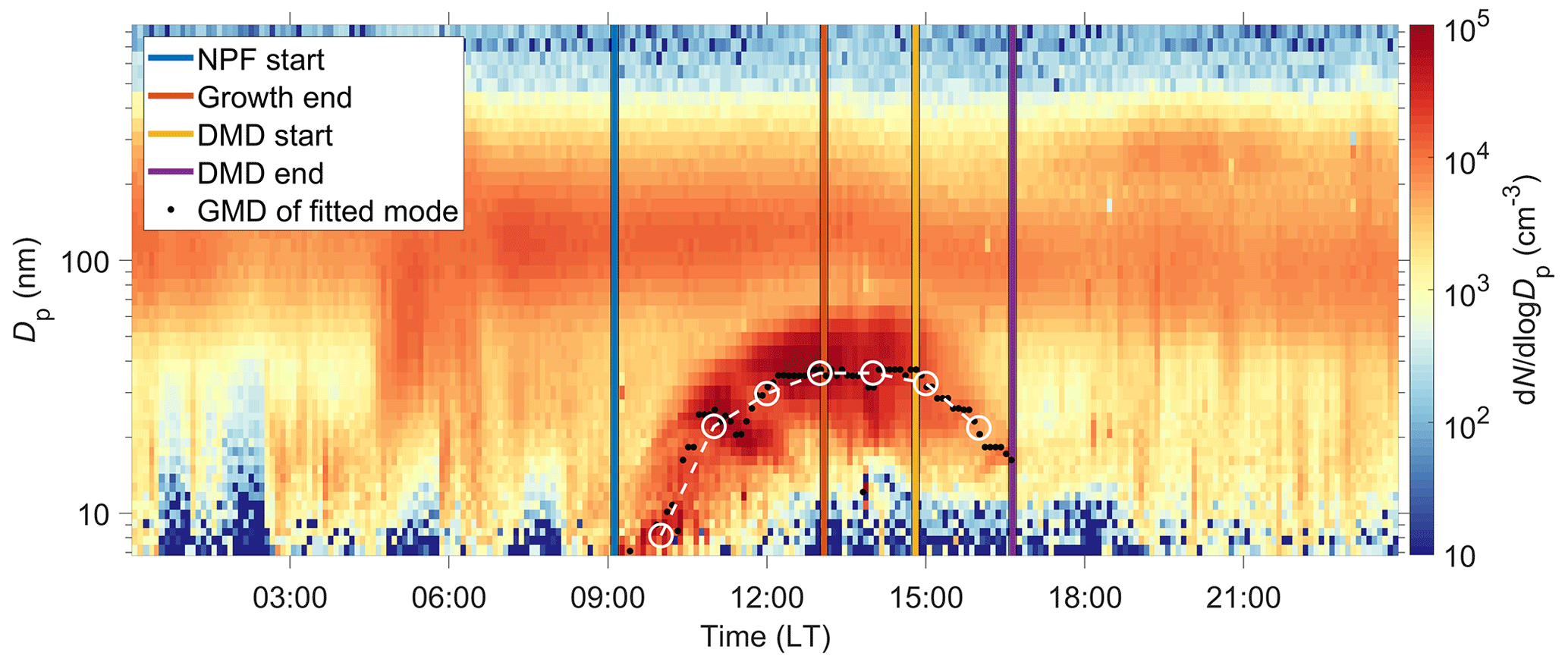
Figure 1Particle number size distribution measured by the DMPS showing an NPF event with a decreasing mode mean diameter (after 15:00 LT; UTC + 3) in Hada Al Sham on 9 July 2013. The figure also illustrates an example of the times describing the progression of the NPF events (colored vertical lines), the geometric mean diameters (GMDs) for the NPF-related particle mode from the fitting algorithm (black dots) and the hourly average diameters used in the model comparison (white circles).
The following points in time were determined visually from the PNSD data to characterize the progression of the NPF events. (1) NPF is first observed in the smallest DMPS size bins (Dp= 7 nm). (2) Clear growth of the mode formed in the NPF event ends. (3) The mode diameter of the newly formed particles starts to decrease. (4) The decreasing mode diameter is no longer observed. These times are referred to as NPF start, growth end, DMD start and DMD end, respectively (Fig. 1). The general criterion in defining the growth end and DMD start times was to find the points in time when both the upper and lower edges of the NPF mode were seen to either increase or decrease simultaneously. On most of the DMD days, the growth end times and the DMD start times are the same. However, sometimes there is a transition period between the clear growth and DMD phases, and in some cases a growing mode and a DMD mode might also be observed simultaneously. In our analysis, the growth and DMD phases are defined as the periods between NPF start and growth end and between DMD start and DMD end, respectively. Therefore, the possible transition periods (between growth end and DMD start) are not included in either of these categories.
In Sect. 4.3, we simulate the NPF event progression using a Lagrangian single-particle growth model and compare the modeled particle diameters against observed ones. In this comparison, the observed diameters are defined using the output of an automated fitting algorithm (Hussein et al., 2005). The algorithm fits log-normal distributions to the measured PNSD data and gives the geometric mean diameters (GMDs) of the fitted distributions. From these, we select the GMDs representing the particle mode produced in an NPF event, apply a robust (outlier-dampening) moving average filter and calculate the hourly geometric mean values. In Fig. 1, the selected GMDs from the fitting algorithm are shown with black dots and the average diameters, used in the model comparison, with white circles connected by a dashed line.
2.3 Air mass history
We use the Lagrangian particle dispersion model FLEXPART (FLEXible PARTicle) v9.02 (Pisso et al., 2019) with ECMWF (European Centre for Medium-Range Weather Forecasts) operational forecast data (0.15° horizontal and 1 h temporal resolution) to compute hourly air mass retroplumes for the study period. In each simulation, 50 000 passive air tracers are released from 0 to 100 m above the location of the measurement site and traced backwards for 3 d. The gridded residence times of the tracer retroplumes are used for estimating the source areas of the NPF-related particles, while the plume trajectories (retroplume centroids) are used in the Lagrangian single-particle growth model (Stohl et al., 2002; Seibert and Frank, 2004).
2.3.1 NPF footprint area
In Sect. 4.2, we utilize the air mass retroplumes to estimate the potential source areas of NPF-related particles. This is done by calculating the locations of air masses, observed at different stages of the NPF progression, at the onset time of the regional NPF event. We refer to this potential source area as the NPF footprint area. In terms of the FLEXPART output, the NPF footprint area for particles observed at tobs is defined as the residence time of the air mass tracers, released at tobs, in the lowest 500 m (a.g.l.) at the backward calculation time of tobs – NPF start. Here NPF start is as defined in Sect. 2.2 but rounded down to the nearest full hour. The rounding-down is done to compensate for the determination of NPF start at Dp= 7 nm, while the actual NPF takes place earlier in smaller particle sizes. Note that interpreting the NPF footprint area as the area where new particle formation took place includes the assumption that regional NPF occurs simultaneously in the whole study domain. However, even if this is not the case, the NPF footprint area is still meaningful in showing the air mass location at the time when NPF was observed to take place around the measurement site.
2.4 Lagrangian single-particle growth model
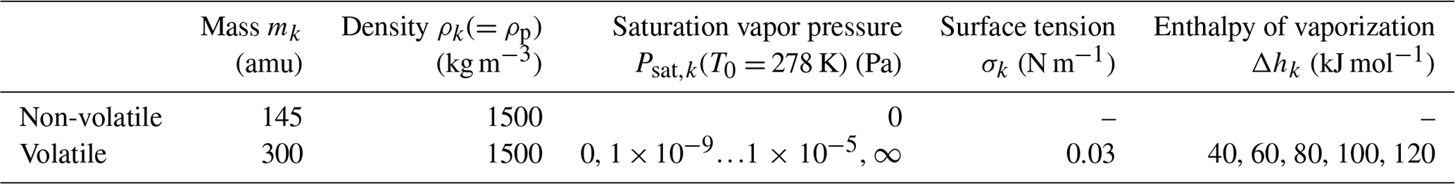
In our model, the idea is to represent particle (formation and) growth within a system consisting of a non-volatile compound and some potentially volatile compound whose evaporation could cause the observed DMD events. The compounds are referred to with the subscripts “non” and “vol”, respectively, and the potentially volatile compound will be referred to as the volatile compound for short. The compounds are also interchangeably referred to as the non-volatile or volatile “species” or “components”, depending slightly on the context. In practice, the non-volatile compound represents sulfuric acid neutralized with base molecules, and the volatile compound represents a low-volatility to semivolatile oxidation product of some anthropogenic organic precursor. Such vapors would produce particles consisting mainly of ammonium sulfate and organic matter, which are reported to be the main components of fine particle mass in the United Arab Emirates (Kesti et al., 2022), representing a similar region to that of our measurements. The relevant values for these compounds are presented in Table 1. Note that, in terms of initial particle formation, the non-volatile compound in practice represents sulfuric acid neutralized with an abundant base stronger than ammonia, e.g., dimethyl amine, which can form effectively stable heterodimers with sulfuric acid and allow for kinetically controlled particle formation without a free energy barrier (Cai et al., 2022). Although the non-volatile assumption is made here mostly due to the lack of measurement data and to simplify the result interpretation, conditions close to these might also prevail in the real atmosphere (Kürten et al., 2018; Cai et al., 2022).
Table 1Properties of the considered compounds in the single-particle growth model. The saturation vapor pressure range of 1 × 10⁻⁹… 1 × 10⁻⁵ Pa is studied using 15 logarithmically spaced values, and it corresponds to a saturation mass concentration range of log10(Csat)= −2.8… 1.2 µg m−3 at T= 300 K using Δhk= 80 kJ mol−1. This covers the transition between low-volatility and semivolatile organic compounds (at log10(Csat)= −0.5) as defined in Donahue et al. (2012).
2.4.1 Formulation of the particle growth rate
An expression for the growth rate of a spherical particle as a function of its mass change rate can be obtained by differentiating the mass expressed as a product of density and volume (Seinfeld and Pandis, 2016):
Here the subscript p refers to particle. mp (kg), ρp (kg m−3) and Dp (m) are the particle mass, density and diameter, respectively. GR (m s−1) is the growth rate (time derivative of the particle diameter). In the derivation of Eq. (1), changes in particle density were assumed to be minor.
Changes in particle mass occur through the collision and coalescence of molecular species or smaller particles with the inspected particle or through the dissociation of material from the particle. In our single-particle growth model, we will not consider particle–particle collisions, and thus we formulate the GR as the condensational growth rate (GRcond; Olenius et al., 2018) using the condensation and evaporation rates of molecular species k, i.e., either non or vol:
Kk,p (m3 s−1) is the collision coefficient between the particle and a molecule of species k. Ck (m−3), γk (s−1) and mk (kg) are the number concentration, evaporation rate and mass of species k, respectively. The evaporation rate γk can be written as
where Kk,p is again the collision coefficient. Psat,k(T) is the temperature-dependent saturation vapor pressure of pure k over a flat surface (Pa; kg m−1 s−2), which is converted into vapor concentration (m−3) by dividing by the Boltzmann constant kB (m2 kg s−2 K−1) and temperature (K). xk is the molar fraction, Γa,k is the activity coefficient and σk is the surface tension (N m−1; kg s−2). The multiplication by the molar fraction in Eq. (3) describes the reduction in the saturation vapor pressure of k in a (dilute) solution according to Raoult's law. The saturation vapor pressure (or evaporation rate) can be further decreased or increased depending on the relative strength of interactions between k and the solvent molecules as compared to those in pure k. This interaction strength is described by the activity coefficient Γa,k. In our calculations, however, Γa,k is set to 1. The last term in Eq. (3), known as the Kelvin term, describes the increasing tendency to evaporate with increasing surface curvature (decreasing particle size) due to the reduced number of neighboring molecules. The temperature dependency of the saturation vapor pressure is expressed with the Clausius–Clapeyron equation:
where Psat,k(T0) is the saturation vapor pressure of pure k over a flat surface at a reference temperature T0. Δhk is the enthalpy of vaporization (J mol−1), which has been assumed to be constant as a function of temperature, and R is the molar gas constant (J mol−1 K−1).
In our growth model, we will only consider collisions between vapor molecules and particles in (or near) the ultrafine range (Dp < 100 nm). Thus, the collision coefficient Kk,p in Eqs. (2) and (3) is approximated using the free molecular regime collision coefficient for hard spheres (Nieminen et al., 2010), with no interactions over distance:
where Dp and Dk are the diameters of the particle and vapor molecule, respectively. and are their mean thermal velocities:
2.4.2 Estimating the concentrations of the condensing species
In the Lagrangian framework, the concentrations of the condensing species need to be evaluated along the air mass transport routes. Essentially, this would require information on the spatial and temporal variability of the species within the whole study domain. As no such measurement network exists, we utilize the satellite-derived [SO2] field to describe the spatial variability of the precursor vapor concentrations and use a simple pseudo-steady-state proxy equation, similar to those in Petäjä et al. (2009), Mikkonen et al. (2011) and Kontkanen et al. (2016), to estimate the concentrations of the condensing species. The same basic formulation, whose assumptions and details are discussed further in the following paragraphs, is used for calculating the spatiotemporally varying concentrations of both the non-volatile (Cnon) and volatile (Cvol) compounds:
Here, [SO2] is the average daytime concentration of SO2 (DU, Dobson units, expressing the atmospheric column burden) for NPF event days from the satellite retrievals (shown in Fig. 6d). The subscript ij represents variable dependency on the latitude and longitude coordinates of a trajectory. “rad” is the calculated theoretical no-sky radiation (W m−2), BLH is the boundary layer height (m) obtained from the ECMWF meteorological data used in the trajectory calculations (based on the bulk Richardson method), and WS and CS are the wind speed and condensation sink (describing the loss rate of the condensing species to pre-existing particles) measured at Hada Al Sham. k is a scaling factor whose value and units depend on the exponents eBLH, eWS and eCS. The value of k is chosen so that the growth from the non-volatile component alone at Cnon=Cij(t) (i.e., fnon= 1 in Eq. 8) exceeds the typically observed growth rates, and the units of k convert the units of the final concentration to molecules per cubic meter. That is, we use the observed PNSD development (growth rate) to constrain the maximum concentration of the non-volatile compound in the absence of gas-phase measurements. The concentrations and relative contributions of both the non-volatile and volatile components are then varied in different model runs by varying the concentration-multiplying factors fnon and fvol in Eqs. (8) and (9). In the case of the volatile component, we additionally vary the saturation vapor pressure and the enthalpy of vaporization (as shown in Table 1) in order to cover the relevant range of condensation–evaporation dynamics.
SO2 is the precursor for the non-volatile component (neutralized sulfuric acid in a system assumed to be saturated with base molecules), and it is mainly emitted from anthropogenic sources. As the volatile (organic) compound is also likely to be of anthropogenic origin, we assume in Eq. (9) that the precursors for the volatile compound have the same spatial distribution as the non-volatile one described by [SO2]ij. This is supported by a similar spatial distribution of the satellite-retrieved formaldehyde (De Smedt et al., 2021), which is an intermediate gas in the oxidation chains of VOCs. The multiplication of [SO2] and rad represents the photochemical production of condensable vapors via OH oxidation, which is likely to be the dominant formation pathway for both sulfuric acid and condensable products from anthropogenic VOCs during daytime (Bourtsoukidis et al., 2019; Srivastava et al., 2022). We do not, however, expect the concentrations of the condensing species to go to zero with the radiation and therefore set a minimum value of 100 W m−2 for the radiation in the calculations after noon, which represents maintained production of the condensable compounds via other oxidation pathways. This roughly corresponds to observations of sulfuric acid concentrations being 1 order of magnitude lower (compared to noon) during non-solar hours, when the production occurs via stabilized Criegee intermediates from the ozonolysis of alkenes (Dada et al., 2020). The same relative strength of the production pathways between the solar and non-solar hours is also assumed for the volatile organic compound, as roughly observed, e.g., in the southeastern US (Krechmer et al., 2015) in a low-NOx and high-radiation environment.
The [SO2] field implemented in the calculations does not vary in time and only represents the total atmospheric column burden of SO2 instead of the surface (or boundary layer) concentration, which are presumably more relevant for our calculations. Because of this, the BLH and WS terms are included to describe the possible variation in the precursor vapor concentrations caused by differing dilution conditions. CS describes the loss of the condensing vapors, which is assumed to be in a pseudo steady state with the production. The strengths of the aforementioned effects are determined by the exponents eBLH, eWS and eCS, which are considered unknown and varied in different model runs. Even though the dilution by BLH and WS would only include negative values for eBLH and eWS in Eq. (7), we extend the inspected range to also include positive exponents. This is partly to account for the fact that the possible diurnal and seasonal variation in the precursor emissions is not included in Eq. (7), which could counteract or change the signs of the exponents in case of similar variability. In addition, the response in precursor concentrations with respect to increasing BLH depends on the unknown vertical distribution of the precursors. Similarly, we extend the range of eCS to negative exponents, since in Hakala et al. (2019) we found the particle formation and growth rates to be positively correlated with CS, which is likely caused by shared sources of precursor vapors and particles acting as the sink. Varying signs and magnitudes for the CS term exponent have been found for similar proxy equations in different environments (Mikkonen et al., 2011). Further regarding the CS term, we wish to point out that using the CS measured at our station is not ideal in the Lagrangian framework, as we do not expect the sink to be horizontally homogeneous. We also note that, in our calculations, the CS term affects both Cnon and Cvol similarly, regardless of the actual saturation ratio of the volatile component.
In addition to the effects explicitly shown and discussed here, we experimented with several other factors that could affect the concentrations of the condensable species experienced by the air mass. These included testing varying exponents for the [SO2] and rad terms, using temporally varying [SO2] fields and applying a concentration dependency based on the height of the trajectory with respect to the boundary layer. We also considered a case where the boundary layer would only affect the concentrations during its growth but not during its collapse. However, none of these was found to improve our results, although not all of the possible combinations of effects were tested.
2.4.3 Modeled particle diameter and the contributions from condensational growth and transport
In our model, the diameter developments of particles arriving at the measurement site at different observation times (tobs) are modeled separately. For a particle observed at tobs, the diameter at time t during its transport is calculated as
where GRcond is the growth or evaporation rate given by Eq. (2), Dp,init is the diameter of the initial “particle” (diameter of the non-volatile vapor molecule, obtained from its mass and density), and Cij(t) is the baseline concentration of condensing species (given by Eq. 7) at the location where a trajectory arriving at the measurement site at tobs is located at time t. Here, new particle formation occurs without a nucleation barrier through the condensation of the non-volatile component onto the initial particle. With larger particle diameters (reduced Kelvin effect), the volatile compound can also contribute to the growth, depending on its saturation ratio. Each day is modeled separately, and t= 0 refers to the zeroth hour of the day. The integration is performed with a 6 min time step to better account for particle diameter and composition-dependent changes, while the particle location and the input data have a 1 h resolution.
The contributions from condensational growth or evaporation (GRtrue) and transport (GRtransport) to the modeled diameter changes between subsequent “observation” times are separated and defined as
Hence, GRtrue is the diameter change rate of the particle observed at tobs, before its arrival at the measurement site, while GRtransport is the difference in the sizes of consecutively arriving particles (particles observed at tobs and tobs−Δt) at the arrival time of the first particle (at time tobs−Δt) divided by the time step. That is, if the particle observed later was already larger or smaller than the particle observed first at the arrival time of the first particle, this difference is attributed to transport, as it originates from the different transport paths taken by the particles. With these definitions, the apparent growth rate in the modeled observations (referred to simply as GRmodel), which conceptually corresponds to the apparent growth rate directly obtainable from the observations, is
as it should be. Note that the common practice of referring to the directly observed diameter changes as growth rates always includes the assumption that the contributions from transport (and coagulation) are zero or negligible, given that the growth rate is understood to be the real diameter change that an individual particle would experience. Here, we use the term apparent growth rate to refer to the observed diameter changes that can include contributions from both the real growth and shrinkage immediately prior to the observations as well as the earlier variations in the growth rate caused by differing environmental conditions along the different transport paths.
2.4.4 Model evaluation metrics
The model performance is evaluated against observations using three different metrics. The three evaluation metrics are the following.
-
Evaluation metric 1: Pearson's correlation coefficient (r) between the logarithms of the hourly observed and modeled particle diameters.
-
Evaluation metric 2: goodness of fit (square root of the coefficient of determination) between the observed and modeled diameter changes with a line passing through the origin during well-defined growth and DMD periods.
-
Evaluation metric 3: exponential of the mean absolute log error between the hourly observed and modeled diameters; i.e.,
The first two evaluation metrics only depend on how well the observed shape of the diameter development is reproduced by the model, irrespective of the actual numerical agreement. The second evaluation metric is specifically included to indicate whether the model is able to produce both increasing and decreasing diameters, as the correlation with a line passing through the origin should not be strong in the case of monotonic growth, while the diameter correlation (metric 1) could still give relatively high values. The third evaluation metric gives the average value by which the model Dp needs to be multiplied or divided in order to arrive at the observed value and therefore assigns the same error for modeled diameters that are a factor of x larger or smaller than the observed ones. This metric depends on the numerical agreement between the observed and modeled diameters and therefore also constrains the concentrations of the condensing species.
In this section, we will briefly summarize some of the relevant results of our previous study, which focused on the general characteristics of NPF at the Hada Al Sham site (Hakala et al., 2019) in order to lay the foundation for the work presented in this study. We will also hypothesize the possible causes of the DMD events based on the previously obtained results. Here, the additional motive is to explain and illustrate the conceptually more complex process resulting in the DMD, which we refer to as the apparent shrinkage process.
NPF events were observed on 73 % of the measurement days (n= 454), and 76 % of these NPF events were further classified as DMD events (Hakala et al., 2019). The frequent occurrence of NPF was found to be linked to the transport of anthropogenic emissions from the coastal regions caused by a highly regular sea and land breeze circulation. The infrequent presence of clouds in the region (Stubenrauch et al., 2010) is also favorable for NPF. Clear nonevent days were only observed when the sea breeze was blocked by strong easterly winds from the inland, preventing the transport of NPF precursors to the measurement site. NPF events were found to start (observed at Dp= 7 nm) a few hours after sunrise throughout the year, and the DMD phase typically started in the afternoon around 6 h after the NPF start. A few hours later, the particles clearly associated with NPF typically disappeared completely from our observations, regardless of whether a clear DMD phase was seen or not. The disappearance of the NPF-related particle mode suggests that NPF is only taking place in a spatially limited area (Hussein et al., 2009). Especially in the DMD cases, the mode disappearance can also be related to the smaller particles being lost to coagulation as a result of increased coagulation efficiency with decreasing particle size. The mean lifetime of, e.g., a 10 nm particle is on the order of a few hours with the typical coagulation sink at the measurement site (10−4 s−1). While there was no clear seasonal variation in the overall NPF frequency, the DMD events were found to be more common during the warmer and windier summer months (Hakala et al., 2019).
Based on the initial result obtained in our previous study, we briefly speculated on the reasons that could be causing the observed DMD events in Hada Al Sham. The first possibility is particle evaporation due to decreasing vapor concentrations and increasing volatility in the afternoon. The decreasing vapor concentrations could possibly be caused by decreasing emissions, increasing sinks, or increasing dilution with increasing wind and BLH in the afternoon. The volatility changes could be related to the changes in temperature. The onset of the DMD events was typically found around the daily maximum temperature, BLH and wind speed (Hakala et al., 2019). Almost all of the DMD events started after the time of maximum solar radiation, when the concentrations of condensable vapors may also decrease due to their decreasing photochemical production rate.
Another possible explanation for the DMD events is a process which we refer to as apparent shrinkage (illustrated in Fig. 2) and in which no real shrinkage of the particles occurs. Apparent shrinkage can be caused by consecutive observations of particles that have grown less during their lifetime than the previously observed particles (Kivekäs et al., 2016). The possibility of this process is supported by the observation that the NPF events seemed to occur only in a limited area whose extent roughly matched that of a high-SO2-concentration area determined from satellite observations (Hakala et al., 2019). Particle formation and growth rates associated with the NPF are expected to decrease when moving further away from the high-concentration area. Thus, particles formed further away from the measurement site are likely to be smaller (at a given time) than those formed in the high-concentration area. Since, on average, we observed no change in the wind direction during the transition from the growth phase to the DMD phase, it is likely that the air masses observed during the DMD phase would have travelled over the same high-concentration areas as the previous air masses. Therefore, in addition to the slower initial growth, the occurrence of the apparent shrinkage requires that the particles observed during the DMD phase also grow less during the transport over the high-concentration areas; otherwise, they would grow at least as much as the previous particles due to the longer growth time resulting from the later time of observation. The lesser growth in the high-concentration area can occur if the particles travel more quickly over the high-concentration area or if the particle growth rates decrease as the day progresses. The decreasing growth rate can be caused by all the same phenomena as discussed above in the context of particle evaporation. However, in the case of particle evaporation, the effects of these phenomena would need to be so strong that not only would the growth rates decrease but they would also become negative. We note that in the initially clean and remote air masses, new particles could also form later in the day (compared to those initially in the high-concentration area) once they are transported over the strong emission sources. Such a delayed NPF start could also result in a DMD event, especially since in this case the total growth time between the formation and detection of the particles would no longer increase as the day progresses if a constant wind speed is assumed.
In summary, for the apparent shrinkage, both conditions (1) and (2) below must be fulfilled by any combination of (a) and/or (b).
-
Air mass in which the DMD is observed must be outside the high-concentration area during the regional NPF event start.
This leads to
- a.
slower initial growth due to lower vapor concentrations or
- b.
later formation of particles once the air mass is transported to an area with sufficiently high vapor concentrations for NPF.
Importantly, in both (a) and (b), the result is smaller (or no) particles in the DMD air mass compared to those initially inside the high-concentration area at any time t.
- a.
-
Particles in the air mass described in (1) must grow less during their transport over the high-concentration area compared to the particles initially in the high-concentration area.
This can be achieved by
- a.
a decreased concentration or higher evaporation rate of condensable vapors in the high-concentration area (possibly caused by enhanced dilution due to increasing BLH and wind speed, reduced production due to weakening photochemistry, decreased emissions, an increased sink, or increased volatility due to increased temperature) or
- b.
faster transport across the high-concentration area (due to increasing wind speed or shifts in wind direction). Note that in this case slower growth in the high-concentration area is not necessary.
- a.
This will allow the particles to be observed at smaller sizes compared to the previous ones, provided that the initial diameter setback in (1) is larger than the additional diameter gained due to the later observation time.
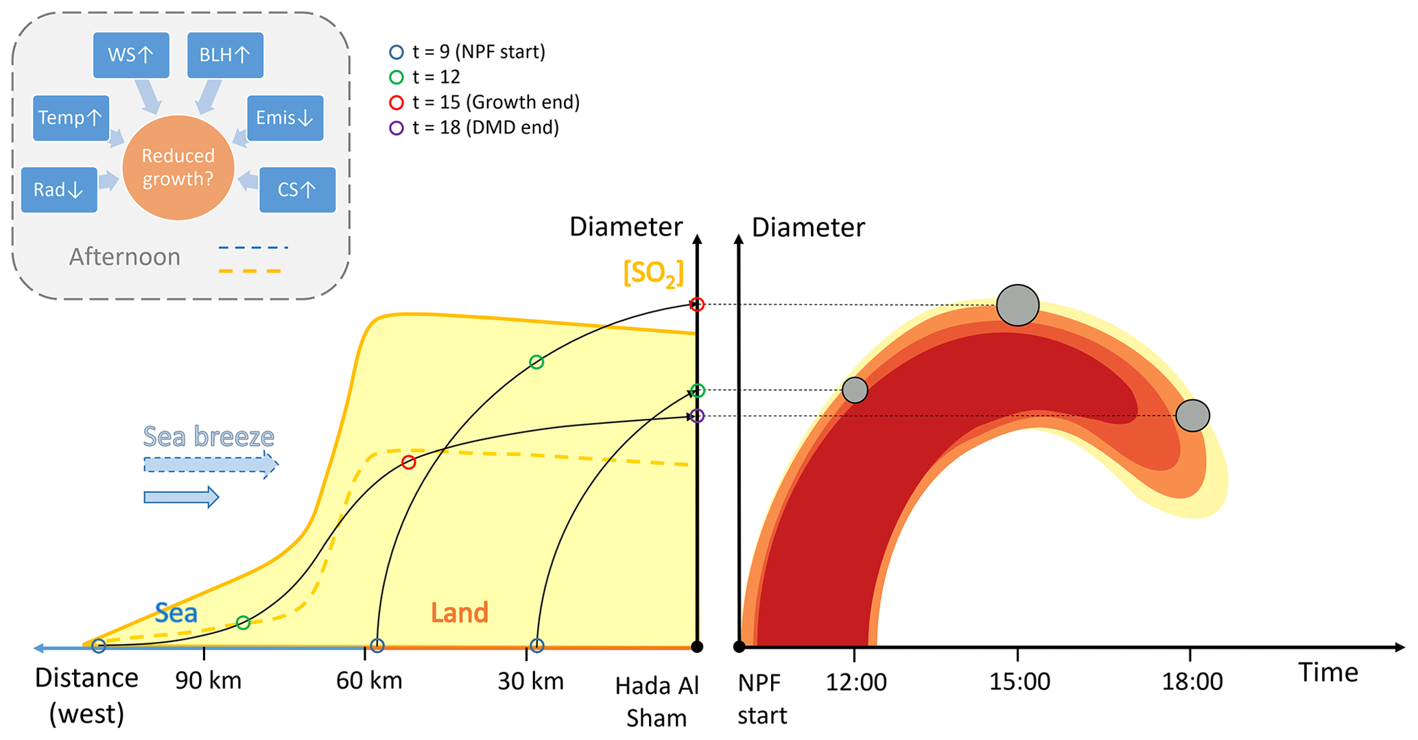
Figure 2A schematic figure illustrating the apparent shrinkage process and the factors possibly contributing to its occurrence. Left panel: longitudinal cross section of the study region with the horizontal axis representing the distance towards the west from the measurement site. The yellow-shaded area represents the average daytime horizontal distribution of the SO2 concentration (vertical axis), which is high over land but drops significantly over the ocean (see Fig. 6d). The black arrows represent particles formed simultaneously at 09:00 in a regional NPF event at different locations. For the arrows, the vertical axis corresponds to diameters of the particles as they are transported towards the measurement site by the sea breeze. The particle diameters and horizontal locations at different times of day are specified with the colored circles. Once the particles arrive at the measurement site (right border of the left panel), their diameters are plotted in the right panel as a function of time to illustrate the observed particle size distribution. In the afternoon, several factors can contribute to reduced growth of particles (see the text and the box in the upper-left corner), which could result in the observation of a decreasing mode diameter even if the individual particles are constantly growing in size.
4.1 Meteorological conditions during growth and DMD periods
If local meteorological conditions and their changes are triggering particle evaporation and causing the DMD events, we expect to find significant differences in these conditions between the DMD and non-DMD cases. We will first compare the average meteorological conditions in the afternoon (12:00–18:00) over the annual cycle between days when NPF events were observed either with or without a DMD phase (Fig. 3; DMD and non-DMD days, respectively). Many of the previous studies on DMD events suggest that temperature and wind speed play major roles in the occurrence of the DMD events (Alonso-Blanco et al., 2017). The significance of the differences between the DMD and non-DMD days in Fig. 3 is evaluated using the Mann–Whitney U test (at the 5 % significance level) separately for each month. Statistically significant differences are highlighted with green shading if they support the speculated causes that could be triggering particle evaporation, i.e., whether temperature, wind speed and boundary layer height are higher or whether the radiation is lower for the DMD days. Statistically significant differences towards the opposing direction are highlighted with red.
Looking first at the temperatures, we find mostly similar conditions between the DMD and non-DMD days, and the only significant difference in February shows higher temperatures on the non-DMD days (Fig. 3a). We can also see that the DMD events can occur even on the lowest-temperature days during the winter. This indicates that the afternoon average temperatures are not a controlling factor in the DMD occurrence in Hada Al Sham. However, we note that even the wintertime temperatures at this site are high compared with many other locations.
In the case of the daytime wind speeds (Fig. 3b), more significant differences are found between the DMD and non-DMD days. The wind speeds are found to be higher on the DMD days in 6 of the 12 months, mostly during the winter. During the generally windier summer months (month nos. 4–9), the number of non-DMD days is overall low, with a maximum of four cases in each month. Examining the fraction of the non-DMD events as a function of wind speed shows some interesting statistics: when the daytime average wind speed exceeds 5.5 m s−1, only ∼ 7 % (7 out of 97) of the NPF days were non-DMD days, whereas with WS < 3.5 m s−1 the fraction is ∼ 70 % (24 out of 35). Therefore, high wind speeds seem clearly favorable for the DMD events, and the seasonal changes in wind speed could possibly explain the higher frequency of the DMD events in summer.
In Fig. 3c and d, we show the boundary layer height (from the ECMWF meteorological data) and the theoretical no-sky radiation. The BLHs are mostly similar, and the significant differences in February and August show higher BLHs on non-DMD days, which does not support stronger (vertical) dilution as a cause of the DMD events. No difference is either seen or expected in the theoretical radiation conditions, and the values are shown here to illustrate the overall seasonal variability.
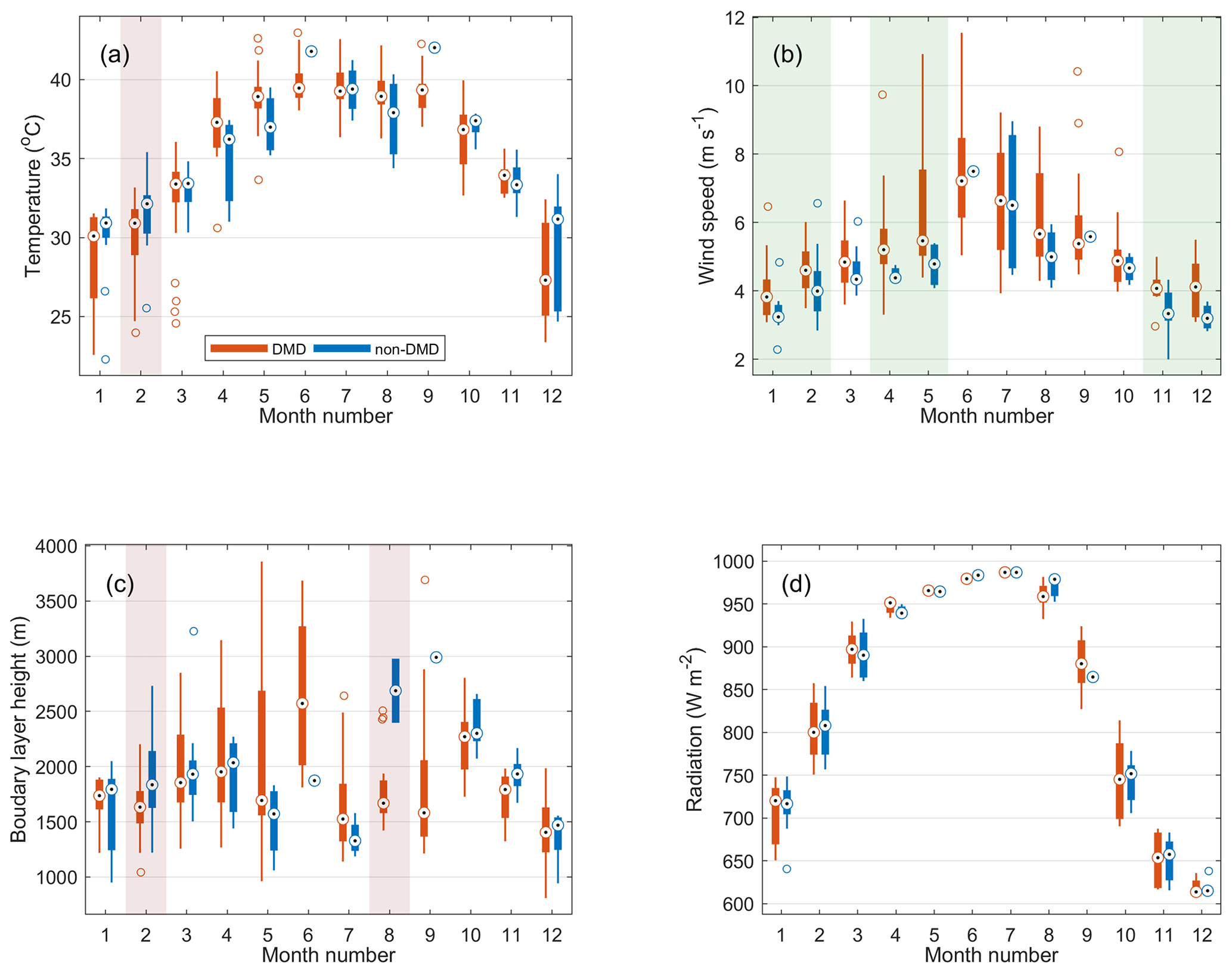
Figure 3Monthly distribution of afternoon (12:00–18:00 LT) mean (a) temperature, (b) wind speed, (c) boundary layer height and (d) theoretical no-sky radiation, separately for DMD days (red) and non-DMD days (blue). The time window is selected to cover the typical onset times of the DMD events (Hakala et al., 2019). Statistically significant differences (one-sided Mann–Whitney U test at the 5 % significance level) between the DMD and non-DMD cases are highlighted with green shading if the difference is in line with the hypothesized triggers for particle evaporation and with red shading for significant differences towards the opposite direction. For each box, the central mark indicates the median, and the bottom and top edges of the box indicate the 25th and 75th percentiles, respectively. The whiskers extend to the most extreme data points not considered outliers, and the outliers (distance from the top or bottom edge of the box more than 1.5 times the interquartile range) are plotted individually using the “o” symbols.
In Figs. 4 and 5, we focus on the diurnal variation in the meteorological conditions (temperature, wind speed, boundary layer height and theoretical no-sky radiation) to obtain a closer look at the potential causes of the DMD events. Similar figures for relative humidity and wind direction are provided in the Appendix (Figs. A1 and A2). In these figures, we do not separate the days into DMD and non-DMD days but instead consider all NPF events and make the separation only based on the current phase (growth or DMD) of the event (see Sect. 2.2 and Fig. 1 for details). In Fig. 4, we compare the conditions of NPF events in the DMD phase with those that still display growth at the same time of day (on another day). In Fig. 5 we focus on the changes in the meteorological conditions, specifically at the onset times of the DMD events, and compare them against the changes on days when growth still continues at the same time. This investigation should more specifically pinpoint any significant differences between the growth and DMD cases. In both figures, the results are shown separately for summer and winter in order to reduce the bias that would arise from the DMD events being more frequent during summer. The significance of the differences is evaluated in the same manner as in Fig. 3.
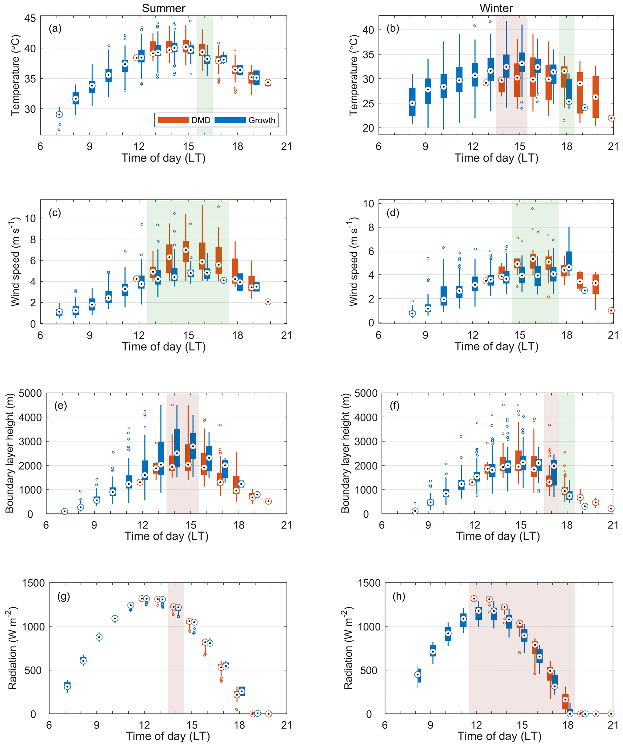
Figure 4Comparison of hourly mean (a, b) temperature, (c, d) wind speed, (e, f) boundary layer height and (g, h) theoretical no-sky radiation between NPF events in the growth phase (blue bars) and DMD phase (orange bars) separately for summer (months: April–September, a, c, e, g) and winter (months: October–March, b, d, f, h). Statistically significant differences (one-sided Mann–Whitney U test at the 5 % significance level) between the DMD and growth cases are highlighted with green shading if the difference is in line with the hypothesized triggers for particle evaporation and with red shading for significant differences towards the opposite direction. For each box, the central mark indicates the median, and the bottom and top edges of the box indicate the 25th and 75th percentiles, respectively. The whiskers extend to the most extreme data points not considered outliers, and the outliers (distance from the top or bottom edge of the box more than 1.5 times the interquartile range) are plotted individually using the o symbols.
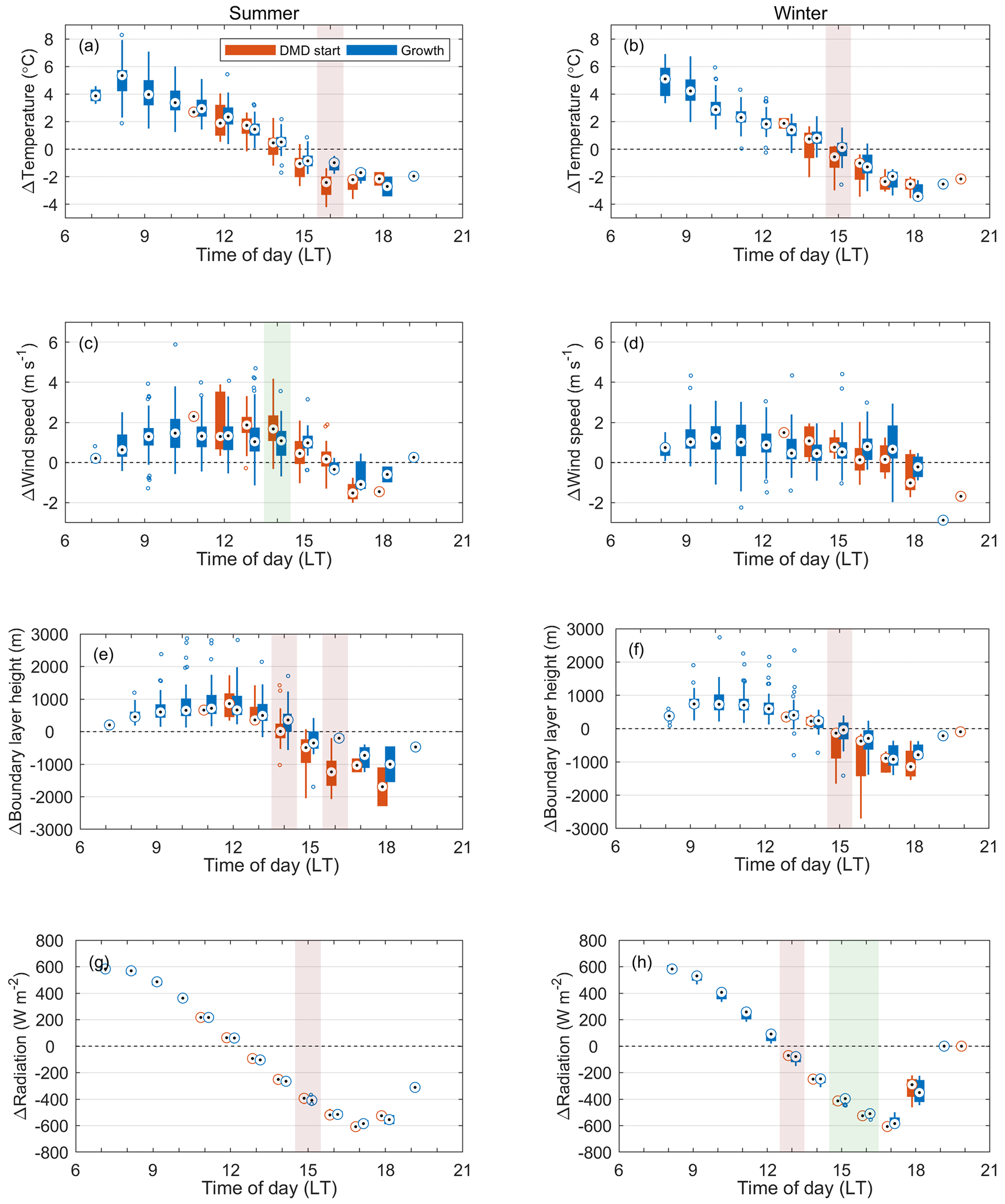
Figure 5Comparison of changes in (a, b) temperature, (c, d) wind speed, (e, f) boundary layer height and (g, h) theoretical no-sky radiation between growth hours (blue bars) and the hours when transition into the DMD phase occurs (orange bars) separately for summer (months: April–September, a, c, e, g) and winter (months: October–March, b, d, f, h). For variable X the change ΔX at time t is calculated as the difference between the hourly means at t+1 h and t−1 h. Values are included in the DMD start category at time t if the DMD start time is found at t ± 0.5 h. Statistically significant differences (one-sided Mann–Whitney U test at the 5 % significance level) between the DMD start and growth cases are highlighted with green shading if the difference is in line with the hypothesized triggers for particle evaporation and with red shading for significant differences towards the opposite direction. For each box, the central mark indicates the median, and the bottom and top edges of the box indicate the 25th and 75th percentiles, respectively. The whiskers extend to the most extreme data points not considered outliers, and the outliers (distance from the top or bottom edge of the box more than 1.5 times the interquartile range) are plotted individually using the o symbols.
The main findings from Figs. 4 and 5 are summarized below.
Temperature is generally not higher during the DMD phase, and in winter it often seems to be even lower during the DMD phase than during the growth phase (Fig. 4a, b). The observed differences in winter should not be due to an uneven representation of different months in the DMD and non-DMD cases since the DMD events are biased towards the warmer months, as confirmed by the higher theoretical radiation on the DMD days (Fig. 4g, h). Changes in temperature during the DMD transition can be either positive or negative, depending mostly on the time of day, and the changes are neither large nor significantly different from those during the growth hours (Fig. 5a, b). The two cases of significant differences (at 16:00 LT in summer and 15:00 LT in winter) show temperatures decreasing more around the DMD start than during growth at the same time. None of these findings supports temperature-driven evaporation as the cause of the DMD events.
Wind speeds are consistently higher during the DMD periods, although in winter slightly less so (Fig. 4c, d). WS is typically increasing around the DMD transition in summer, but in winter this is less clear (Fig. 5c, d). The change is typically not significantly higher around the DMD start than during the growth hours. The higher wind speed during DMD could support dilution-driven evaporation or DMD by transport of particles from further-away regions, as the higher wind speeds leave less time for particles in the DMD air masses to grow as they travel over the high-concentration areas. Wind direction is typically from the east during the day, but the DMD phase shows some preference towards northeasterly winds, while southeasterly winds are more common during the growth hours (Fig. A1c, d). No clear differences are seen in the change in wind direction around the DMD onset times (Fig. A2c, d).
BLH is generally lower during the DMD phase, especially in summer (Fig. 4e, f). The DMD start times can be associated with both increasing and decreasing BLH (Fig. 5e, f). The significant differences show smaller increases and larger decreases in the BLH during the DMD transition. These results do not support DMD being caused by increased vertical mixing.
In the case of the theoretical no-sky radiation (Figs. 4g, h and 5g, h), any significant differences are a result of uneven distributions of the cases between the different months. The theoretical radiation values are shown to display that radiation is almost always decreasing during the DMD phase, and thus the reduced photochemical production of condensable vapors could contribute to the DMD events. However, decreasing radiation at some point during the NPF progression happens with most regional NPF events around the world, and this does not systematically trigger DMD events. Also here, the growth phase often continues even after the radiation starts to decrease, and some of the DMD events are found to start while the radiation is still increasing.
Overall, the only consistent difference in the meteorological conditions is the higher wind speeds on the DMD days and during the DMD phase. However, since (1) the magnitude of the difference is quite small compared to the growth cases, (2) the DMD onset is not related to any unusually large changes in WS, (3) the wind direction does not change significantly during the transition and (4) the BLH is not consistently higher or increasing significantly, we consider it unlikely that a wind-driven increase in dilution would be enough to trigger significant particle evaporation. The role of evaporation in the DMD events is still examined further in Sect. 4.3 using the Lagrangian single-particle growth model. In the next section, however, we will inspect the prerequisites for the transport-driven apparent shrinkage process.
4.2 NPF footprint areas for the growth and DMD phases
In Sect. 3, we speculated that in order to produce apparent shrinkage, the air masses observed during the DMD phase would need to be located outside the region of high precursor concentrations at the onset time of NPF. That is, the NPF footprint area (as defined in Sect. 2.3.1) of the particles observed in the DMD phase should lie in the less polluted regions. The fruition of this condition is studied in Fig. 6.
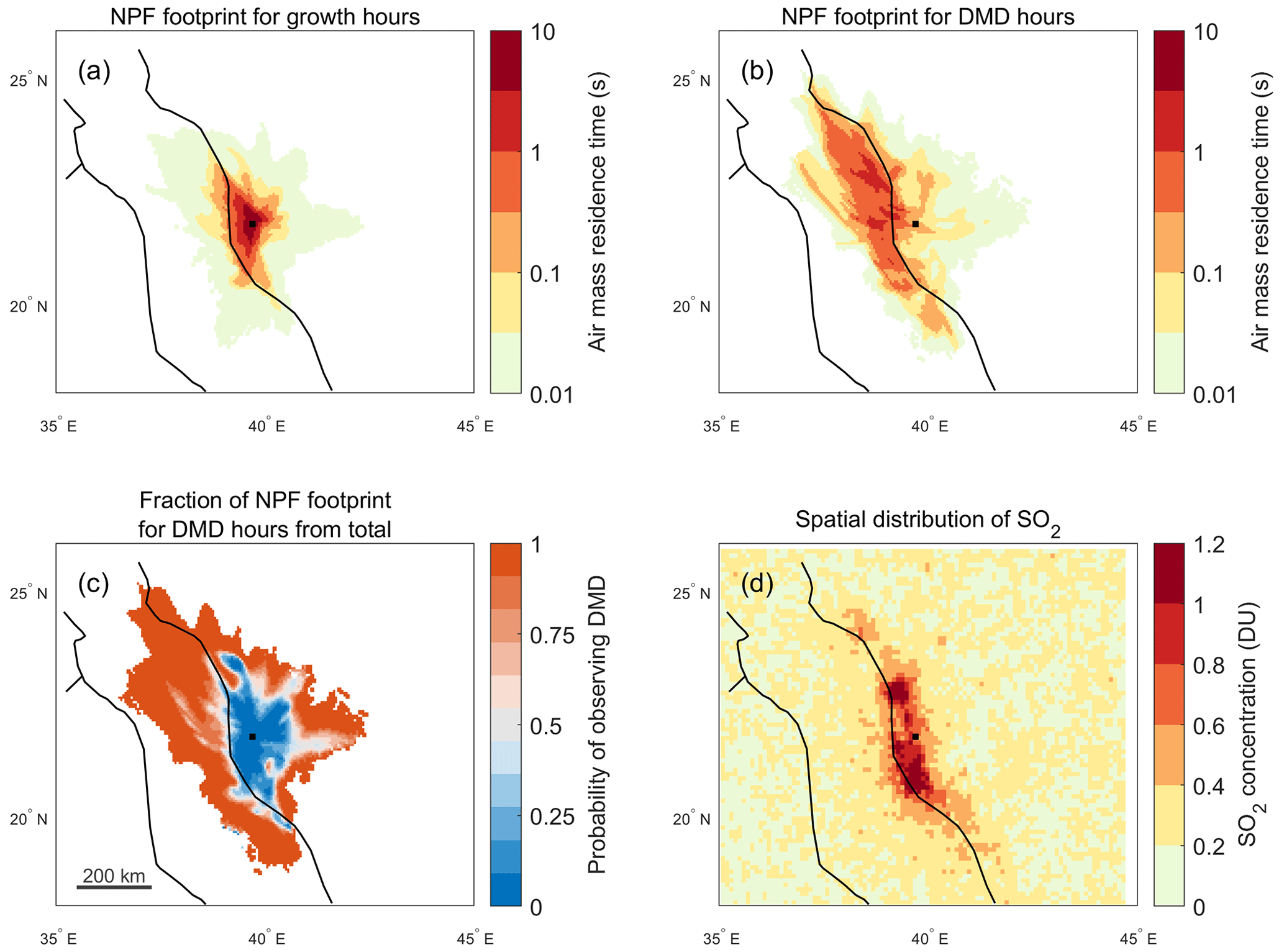
Figure 6Average NPF footprint areas (see Sect. 2.3.1) for (a) growth hours and (b) DMD hours. Panel (c) shows the fraction of the (non-averaged) NPF footprint of the DMD hours from the total NPF footprint (growth + DMD). The result in panel (c) corresponds to the likelihood of observing DMD at the measurement station with respect to the air mass location at the onset time of NPF. A value of 1 means that air masses located in these regions at the onset time of NPF will always result in a DMD once transported to the measurement site, provided that a mode related to an NPF event is observed. Conversely, a value of 0 means that particle growth is always observed. In panel (d) the average SO2 column concentration (1 DU = 2.69 × 10¹⁶ molec. cm−2), obtained from the OMI Level 2 SO2 planetary boundary layer product (Li et al., 2013), in the surroundings of Hada Al Sham during NPF days is shown.
In Fig. 6a and b, we show the NPF footprint areas for the growth and DMD phases, respectively. In order to illustrate the transition region between these cases more clearly, we show the fraction of the NPF footprint for DMD from the total NPF footprint in Fig. 6c. In Fig. 6c, the values are related to the probability of observing DMD at the measurement site with respect to the air mass location during NPF start. The NPF footprint area for the growth hours and the probability of observing an NPF event in the growth phase show a clear resemblance to the areas of high SO2 concentrations shown in Fig. 6d. By contrast, the DMD footprint and the probability of observing an NPF event in the DMD phase are very much focused on the cleaner regions, mainly above the ocean (note the logarithmic axis in Fig. 6a and b). Towards the west, the transition consistently occurs along the coastline, where the concentration of SO2 is seen to drop significantly. Towards north and south, the growth-favoring region extends clearly further, consistent with the high-concentration region. This implies that the smaller particles observed during the DMD phase are indeed formed in initially less polluted air masses, in line with the first hypothesized condition that would be needed for the apparent shrinkage process (see Sect. 3).
However, in order to produce a DMD, lesser growth during transport over the high-concentration area would additionally be required (the second hypothesized condition in Sect. 3). The higher wind speeds observed during the DMD phase (Fig. 4c, d) already provide a possible explanation for the lesser growth, as they contribute to shorter residence times over the higher-concentration area and potentially dilute the concentrations as well. While the behavior of temperature and BLH did not seem to support evaporation (or reduced growth) at the measurement site during the times when the DMD was observed to take place, they might still contribute to evaporation or reduced growth at different times during transport. In the following section, we consider the spatiotemporal variability in the conditions that could modulate aerosol growth during air mass transport and study their effects on the resulting particle size distribution using a Lagrangian single-particle growth model.
4.3 Modeling the NPF development with a Lagrangian single-particle model
In order to get a more complete picture of the processes contributing to the DMD events, we develop a Lagrangian single-particle growth model utilizing the available data (see Sect. 2.4) and apply it to model the diameter development of newly formed particles on NPF event days. In short, the model considers the condensation and evaporation of two species, of which one is completely non-volatile (representing neutralized sulfuric acid) and the other is potentially volatile (representing some low-volatility to semivolatile organic compounds of anthropogenic origin). Overall, the model relies on the assumption that the general spatial distributions of the precursor vapors for both the non-volatile and volatile species are described by the satellite-retrieved SO2 distribution (shown in Fig. 6d) and that the production of the condensable vapors from the precursors depends linearly on radiation. Additionally, we consider the possible modulating effects of BLH, WS and CS on the vapor concentrations, but both the magnitudes and directions of these effects (i.e., the exponents eBLH, eWS and eCS in Eq. 7) are treated as unknowns. Due to no measurement data, the true concentrations and properties of the condensing species are also unknown, but the measured particle size distribution constrains the space of possibilities and can be used to infer the more likely effects and conditions. In practice, our approach is to perform a multitude of model runs with varying model configurations in order to find the best-performing description, determined by the model evaluation metrics (described in Sect. 2.4.4). If we then assume this description to be the most likely representation of the real case, we can disentangle the contributions from evaporation and transport as well as the factors affecting their occurrence.
4.3.1 Finding the best-performing model configuration
The results of our model evaluation are presented in Figs. A3–A6 in the Appendix and in Fig. 7 in the main text. In detail, the model evaluation proceeds by first setting all the exponents eBLH, eWS and eCS in Eq. (7) to zero and the concentration multiplier fvol and enthalpy of vaporization Δhvol of the volatile component to 1 and 80 kJ mol−1, respectively. We then vary each of the exponents (in the order stated above) and inspect the model performance based on the evaluation metrics over the full possible range of concentrations of the non-volatile component (from 0 to values where the non-volatile condensation alone overestimates the growth, represented by the range of fnon = 0 … 1) and saturation vapor pressures of the volatile component (from fully volatile to non-volatile, with a specific focus on the low-volatility to semivolatile range, represented by the range of 0, 1 × 1, ∞ Pa). From Figs. A3, A4 and 7, which show the performance with varying eBLH, eWS and eCS, respectively, we can see that any single evaluation metric displays improvement or deterioration over the full range of fnon and Psat,vol(T0) and that the responses of the different evaluation metrics correlate with one another with the varying exponents. This makes the selection of the best-performing exponents straightforward, and the obtained values are eBLH = 0.5, eWS = 0 and eCS = −0.5. We will next discuss the implications of the obtained exponents and then inspect the effects of varying fvol and Δhvol, which result in more subtle changes in the model performance (Figs. A4 and A5).
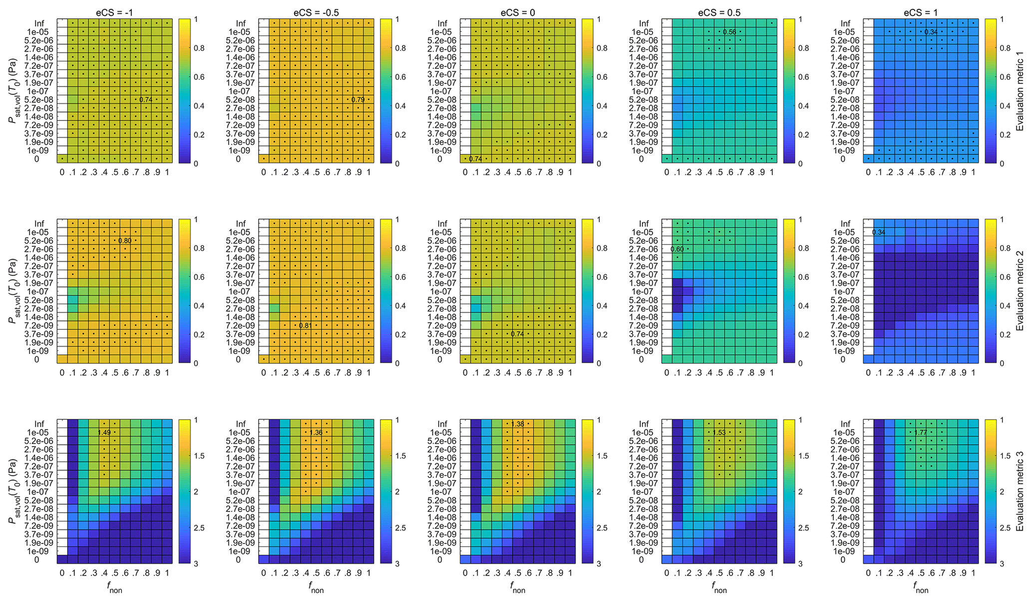
Figure 7Evaluation of the model performance with different exponents for the condensation sink term (eCS) when eBLH = 0.5, eWS = 0, fvol= 1 and Δhvol= 80 kJ mol−1. Each column of panels contains the performance matrices of the three evaluation metrics (see Sect. 2.4.4 for explanations of the metrics) as a function of the concentration multiplier for the non-volatile compound (fnon) and the saturation vapor pressure of the volatile compound (Psat,vol(T0)) with a specific eCS value. In the first two rows, higher correlation values of the evaluation metrics indicate better model performance, while in the last row, lower deviations correspond to better results (better results are always towards the yellow colors). In each panel, the value of the evaluation metric for the best model performance is shown in numbers. Values close to the best one (difference less than 0.015 in the correlation values and less than 5 % in the deviation value) are highlighted with black dots. Each model run, resulting in a single data point for each of the evaluation metrics, comprises 138 NPF event days.
The positive exponent for the BLH term produces higher vapor concentrations with increasing BLH. This is in contrast to the expected effect of increasing dilution by increasing boundary layer height but matches the observations of generally lower BLH during DMD events found in Sect. 4.1. Positive exponents for the BLH term could result from the residual layer containing similar or higher amounts of precursor vapors than the mixing layer or by the CS being diluted relatively more with increased vertical mixing than the precursor vapors. Such a situation could potentially arise from the consistent sea breeze circulation in the study region (Parajuli et al., 2020) and elevated stack emissions over the shallow nocturnal boundary layer (Ukhov et al., 2020b), with additional contributions from the higher dry deposition velocities of gases compared to particles in the ∼ 100 nm range that control the CS (Seinfeld and Pandis, 2016). In the United Arab Emirates, Kesti et al. (2022) report indications of elevated layers with high SO2 concentrations as the surface concentrations often increase with entrainment from the residual layer. Recent modeling studies over China have also suggested that more favorable conditions for new particle formation and growth, including higher concentrations of precursor vapors and oxidants as well as a lower sink and temperature, might exist higher up in the atmosphere, causing increased vertical mixing to result in enhanced particle formation at the surface (Lai et al., 2022a, b). However, in our case the positive eBLH could also be related to the diurnal and/or seasonal variation in emissions, which are not considered in the model, through the increase in both BLH and emissions with temperature in a region where energy consumption responds to the need for air conditioning (Ukhov et al., 2020b). An increase in the BLH value during transport may also signal the arrival of an air mass, initially located over the sea, over land areas, where the magnitude in the diurnal variation of BLH is much stronger. Considering this, the positive eBLH could stem from the concentration gradient between land and sea being stronger in reality than described by the satellite-retrieved distribution used here. However, we also briefly tested higher exponents for the [SO2] term, which result in an increased contrast between the high- and low-concentration areas, but this did not yield improved results. While several possible explanations for the positive eBLH exist, we are unable to pinpoint the underlying effects.
Higher wind speed was found to favor the occurrence of DMD events in Sect. 4.1. The obtained zero exponent for the WS term here suggests that this connection is related to transport effects rather than dilution effects. This is because the transport-related effects of wind speed are inherently included in the Lagrangian framework via the use of air mass trajectories, and thus their contribution is not expected to show up in the exponent here (whereas the dilution effects would be). While the wind conditions will certainly modulate the precursor concentrations to some degree, it seems that the major influence of wind speed comes from its effect on the air mass travel time over the high-concentration area.
The negative exponent for the CS term is in contrast to the expectation of decreasing concentrations of condensing vapors with an increasing sink. However, it is not completely unexpected at this particular site, as we previously found particle formation and growth rates to be positively correlated with the CS (Hakala et al., 2019). We believe this to reflect the common anthropogenic sources of NPF precursor vapors and large (possibly primary) particles that mainly control the CS. That being said, faster particle growth over the anthropogenically active areas should ideally be already accounted for by the [SO2] field without the need for additional input from the observed CS. As such, the improved model performance when using eCS = −0.5 might act to correct some of the errors that undoubtedly arise from the highly simplistic description of the precursor vapor distribution and the representation of the air mass movements by the trajectories. Since the measured CS is expected to increase as a result of particle growth, it might provide direct input on the intensity of condensation that is not otherwise captured by the model.
In terms of changing the concentration multiplier (fvol) and the enthalpy of vaporization (Δhvol) for the volatile component, the responses in the overall model performance are much less pronounced (Figs. A5 and A6). Varying either of these does not significantly affect the best model performance within any metric but mostly shifts the regions in which a similar model performance is found. The shifting of the regions is expected, as largely analogous conditions are obtained by combining higher concentrations of the volatile component with higher saturation vapor pressures and higher enthalpies of vaporization with lower saturation vapor pressures (the slope of the saturation vapor pressure curve with respect to temperature increases with increasing Δhvol, and thus, in order to reach similar Psat,vol(T) values at a specific T > T0, a lower initial Psat,vol(T0) is needed). The conditions are, however, not exactly the same as both the fvol and Δhvol can affect the timing and intensity of the condensation–evaporation dynamics over the diurnal cycle, with a higher fvol essentially promoting more intense condensation and evaporation and a higher Δhvol making the saturation vapor pressure more sensitive to the diurnal variation in temperature. From Fig. A5 we can see that, while the best model performance is not affected by the choice of fvol, the worse-performing regions deteriorate with increasing fvol. This suggests that strong contributions from the volatile component are not favorable for the model performance. The very low overall model sensitivity to variations in Δhvol (Fig. A6) in turn signals that the changes in the concentrations of the volatile component dominate over the temperature-dependent changes in the saturation vapor pressure over the diurnal cycle. As such, the choice of the value of Δhvol seems largely inconsequential in terms of further analysis, while choosing the value of fvol still requires further considerations.
In the next section, we will focus on the model performance between individual model runs with specific concentration multipliers of the non-volatile component (determined by fnon) and saturation vapor pressures of the volatile component Psat,vol(T0). The discussion is based on the results shown in the second column of Fig. 7, which are considered to represent the best-performing model configuration: eBLH = 0.5, eWS = 0, eCS = −0.5, fvol= 1 and Δhvol= 80 kJ mol−1. As mentioned, the value of fvol is still discussed further.
4.3.2 Contributions from the volatile and non-volatile components
In the previous section, we found the best overall model performance (with any fnon and Psat,vol(T0)) when eBLH = 0.5, eWS = 0, eCS = −0.5 and Δhvol= 80 kJ mol−1 (and fvol= 1) (Fig. 7). Here we will discuss the results in terms of varying contributions from the volatile and non-volatile components, determined by fnon and Psat,vol(T0), respectively. In general, we find quite low sensitivity to changes in fnon and Psat,vol(T0) in the first two model evaluation metrics (Fig. 7, first two rows), which depend only on the shape (and not the absolute values) of the modeled diameter development. However, a band of poorer performance that covers a specific Psat,vol(T0) range and extends towards higher volatilities with increasing fnon can be seen especially in the second evaluation metric. The same region was found to be more pronounced with higher fvol (Fig. A5). In this region, the condensation–evaporation dynamics of the volatile component are particularly sensitive to the saturation vapor pressure. This can be inferred from the fact that above and below this region the behavior resembles that of completely volatile and non-volatile vapors, respectively, as seen from the similar values to the cases of and 0. This shows that some combinations of fnon and Psat,vol(T0) lead to semivolatile dynamics that do not match the observed shape of the particle diameter development, while a wide range of conditions produce results close to the best obtained values.
The third evaluation metric (Fig. 7, third row), which reflects the numerical agreement between the observed and modeled diameter values, naturally places much stricter limits on the choice of fnon and Psat,vol(T0). With no contribution from the volatile component (), we find a local maximum in the performance with fnon= 0.5. Note that this local maximum is very close to the global maximum found at fnon= 0.5 and 1 × 10⁻⁵ Pa, which we will later show to represent practically non-volatile condensation with a negligible contribution from the volatile component. With fnon > 0.5, the contribution from the non-volatile component already exceeds the typically observed particle diameters, and thus the model performance decreases monotonically with an increasing contribution from either the non-volatile or volatile component. Therefore, the region of interest lies in the values of fnon≤ 0.5, where a decreasing contribution from the non-volatile compound needs to be compensated for by an increasing contribution from the volatile compound. However, when looking at the performance of the third evaluation metric in Fig. 7, we quickly come to realize that the increasing need for the volatile compound (decreasing fnon) simultaneously results in worse model performance, regardless of the chosen Psat,vol(T0). This is related to the fact that, in order to get a quantitatively suitable contribution from the volatile compound when fvol= 1, its Psat,vol(T0) needs to lie in the range where the condensation is clearly modulated by the saturation vapor pressure; with very high Psat,vol(T0), no condensation will occur, and the resulting particles will be too small (especially when fnon≤ 0.3), whereas with very low Psat,vol(T0), the condensation will approach that of a non-volatile compound, which will produce overly large particles if fvol = 1. This is because a non-volatile compound alone already produces overly large particles with > 0.5, as discussed above. However, this same semivolatile regime, where the volatile component needs to lie, was found to worsen the model performance, especially in terms of the second evaluation metric, indicating a poorer match in the shape of the modeled particle diameter development with the observations.
The “problem” of having to place the volatile component in the semivolatile regime can, of course, be circumvented by using an fvol value lower than 0.5. However, in this case the best model performance is found when the volatile component simply behaves as another non-volatile one, as can be seen from the case of fvol= 0.2 in Fig. A5. In this case, no evaporation is possible. The fvol range between 0.2 and 0.5 was further studied with small increments of 0.05 to confirm that the best performance is never found in the semivolatile regime (Fig. A7). Thereby, any significant contribution from a truly semivolatile component does not aid in reproducing the observed diameter development with our model. This suggests that the evaporation of a volatile compound is unlikely to be an important contributor to the DMD events.
Based on the results and discussion above, we deem the case of fnon= 0.5 and 1 × 10⁻⁵ Pa (with eBLH = 0.5, eWS = 0, Δhvol= 80 kJ mol 1; Fig. 7) to be representative of the best-obtainable results by our model. The strong correlation between the modeled and observed diameters and their changes (r= 0.79 and r= 0.80, evaluation metrics 1 and 2, respectively) and the modeled particle diameters being on average within a factor of 1.36 from the observed ones (evaluation metric 3) indicate good performance of the model. In the next section, we will illustrate the model-produced particle diameter development and address the causes of the DMD events more specifically.
4.3.3 Contributions from evaporation and transport
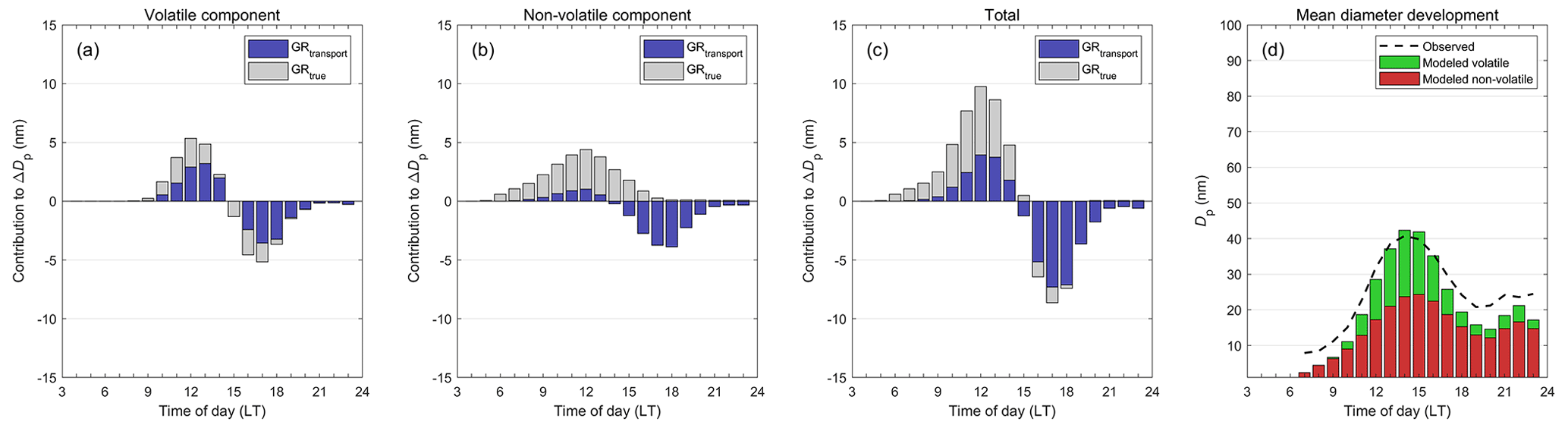
In Figs. 8 and 9, we illustrate the development of the observed and modeled mean particle diameters together with the modeled contributions from true diameter changes and transport effects (see Sect. 2.4.3) for two cases chosen based on Fig. 7. In Fig. 8, we show the case of the best model performance (fnon= 0.5 and 1 × 10⁻⁵ Pa), while in Fig. 9 we illustrate an example of a case where the non-volatile component alone is clearly insufficient in explaining the observed particle diameters (here fnon= 0.3, 5.2 × 10⁻⁸ Pa). In the latter case, a clear contribution from the volatile component is needed, which results in a poorer model performance.
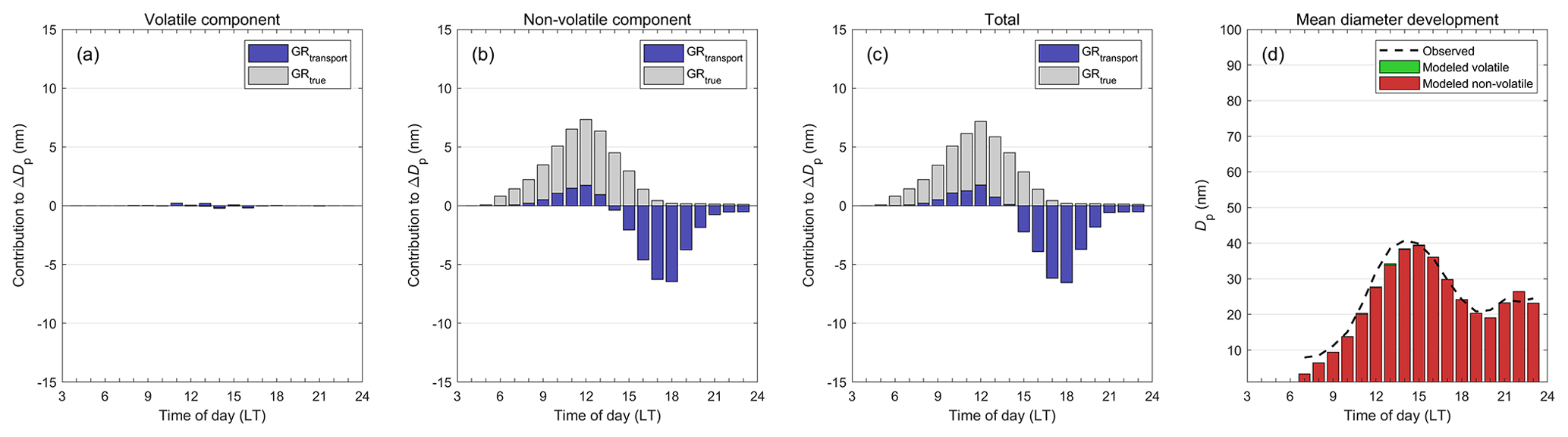
Figure 8Mean contributions to modeled diameter changes by (a) the volatile component, (b) the non-volatile component and (c) both the volatile and non-volatile components when using the best-performing model configuration (eBLH = 0.5, eWS = 0, eCS = −0.5, Δhvol= 80 kJ mol−1, fvol= 1, 1 × 10⁻⁵ Pa and fnon = 0.5). The diameter contributions are separated into contributions from true diameter changes (GRtrue; condensation, evaporation) and transport (GRtransport) described in Sect. 2.4.3. (d) Observed and modeled mean particle diameter. All the panels contain data from 138 NPF event days. In panel (d), only hours when the observed mode diameter is defined are included.
From Fig. 8 we can see that in the case of the best model performance, the contribution from the volatile component is on average negligible. Despite this, the mean diameter development – including the DMD behavior – is reproduced remarkably well. With the non-volatile component, no evaporation is possible, and thus the DMD events are caused by the apparent shrinkage process. In this process, the decreasing size of the observed particles results from differing conditions during transport, as directly shown by the strongly negative contributions from GRtransport to the diameter changes, especially in the afternoon (Fig. 8b or c). In addition to the negative contribution from transport, we can also see a smaller positive contribution during the earlier growth hours. This is caused by the generally increasing concentrations of the precursors from the immediate vicinity of the measurement site towards the high-emission areas along the coast (Fig. 6d). Therefore, according to the model results, calculating particle growth rates directly from the observed size distribution would typically give an overestimate of the real condensational growth at the measurement site during the early hours. However, a much more severe misjudgment would be made if the DMD events were similarly interpreted as representing net evaporation of particles, since the true diameter changes in individual particles are continuously positive.
If we choose a worse-performing model configuration where a significant contribution from the volatile component is needed, net evaporation of the volatile component is also found to contribute to the diameter changes (Fig. 9a). The evaporation peaks around 16:00 LT, when the photochemical production rate has significantly dropped from its midday maximum while the temperature is still around its highest values (see Fig. 4). However, while evaporation can be significant for the volatile component, in the total contributions some of the evaporation is compensated for by simultaneous condensation of the non-volatile compound, and overall the DMD is still predominantly caused by transport in the displayed case. The relative contributions of the different terms are obviously dependent on the chosen value of fnon, but we remind the reader that the overall agreement between the observations and the model was found to weaken with decreasing fnon. With lower fnon and a higher contribution from a semivolatile compound, both the early morning and late evening diameters become progressively more underestimated, while the daily maximum diameters are overestimated due to the strong diurnal variation in the condensation–evaporation dynamics of the semivolatile component. Such variation is not in line with the observed diameter development, making significant contributions from volatile compounds and evaporation seem unlikely.
4.3.4 Hypotheses vs. model results
Lastly, we comment on the hypothesized causes of the DMD events presented in Sect. 3 based on the obtained model results. We found that effectively non-volatile condensation best explains the observations. This suggests that the DMD events are caused by the apparent shrinkage process enabled by differing conditions during transport. In Fig. 10, we illustrate these differing conditions in terms of the concentration of the non-volatile component and the contributing factors for the daily largest and smallest modeled particles using the best-performing model configuration. In agreement with the first hypothesized condition for the apparent shrinkage (Sect. 3), we found that the particles observed during the DMD phase are located outside the high-concentration region around the onset of NPF (Fig. 6). This can also be seen from Fig. 10b and identified as a major contributor to the DMD events, since most of the diameter difference (reflected by the integral of the concentration difference in Fig. 10c) between the daily largest and smallest particles results from the DMD air mass being located in the lower-concentration area until 14:00 LT. In addition to the lower [SO2], the lower BLH in the DMD air mass also contributes to the slower initial growth in our model.
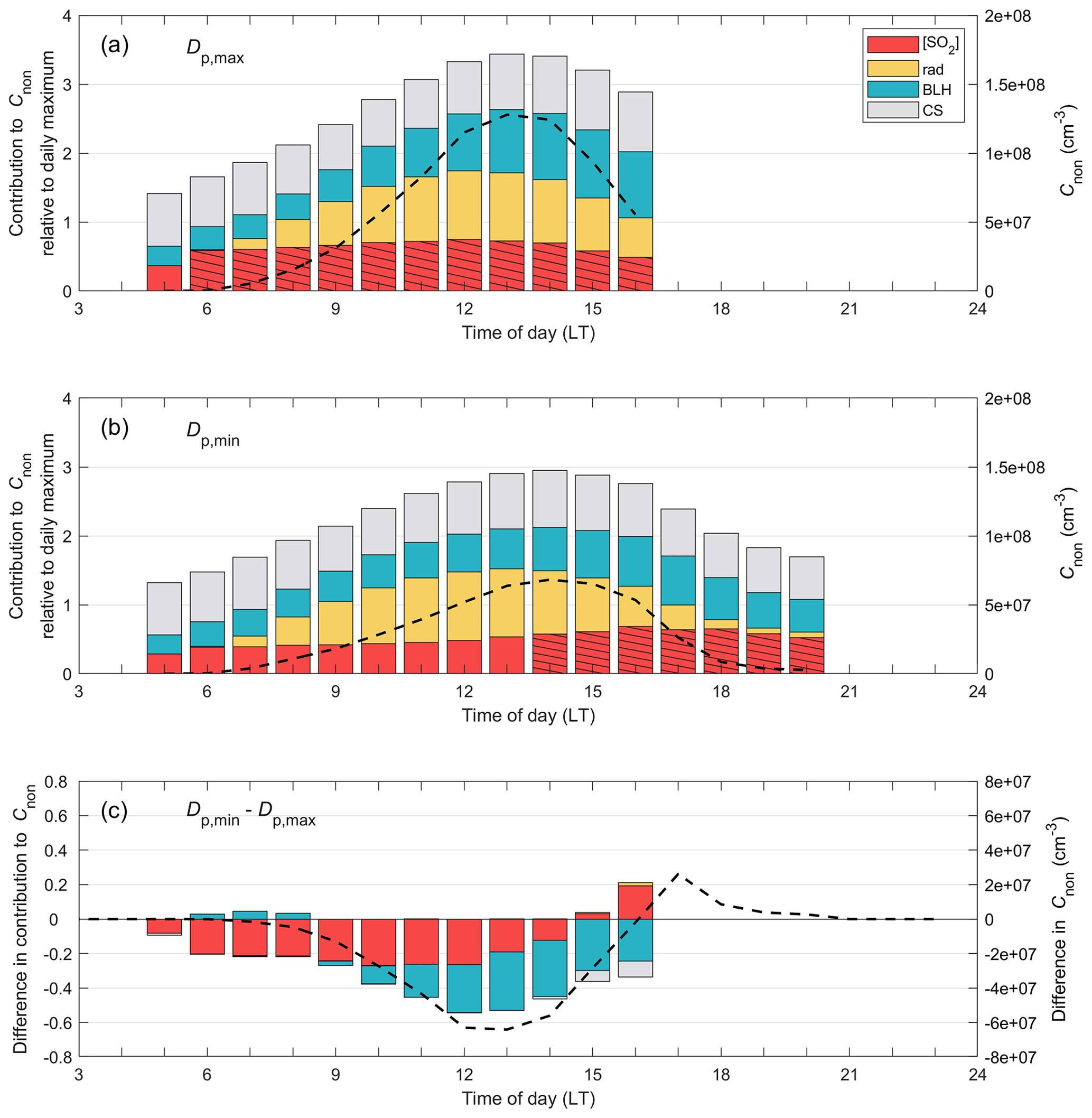
Figure 10(a, b) Left axis (bars): mean contributions of the different factors (relative to the daily maximum) affecting the calculated concentration of the non-volatile component (Cnon) during air mass transport to the measurement site. Right axis (dashed black line): the concentration of the non-volatile component (note that the concentration responds to the product of the different factors). In panel (a), we show the mean conditions resulting in the daily largest modeled particle (Dp,max) and in panel (b) the mean conditions resulting in the smallest modeled particle in the evening (Dp,min) during the time when the NPF-related mode is still observed in the measurements. Only the most typical arrival times for the largest and smallest particles are considered (n > 10; hours 13–16 for the largest particles and hours 17–20 for the smallest particles). The dashed bars mark the times when the air masses are typically located over the high-concentration area (here defined as [SO2] > 0.55 DU). (c) The difference between the conditions resulting in the smallest and largest particles (b) − (a). The concentration line in panel (c) is also shown after 16:00 LT to display the small positive contribution from the additional growth time compared to the negative contribution resulting from less favorable conditions for growth during transport. The difference in the sizes of the smallest and largest particles at a given time is reflected by the integral of the concentration difference in panel (c) up to that time.
We are not able to comment on whether in reality the later NPF start or the slower growth in the initially cleaner air masses (subpoints of the first hypothesized condition in Sect. 3) is the main cause of the initial setback in the diameter development. This is because in our model any non-zero value of radiation will simultaneously initiate particle growth everywhere, regardless of the SO2 concentration. Thus our model only considers the first option, while in reality, slowly growing particles formed far away from the measurement site could be lost to coagulation before they reach our observations. Therefore, particles formed later in the day closer to the measurement site might also be relevant.
In Sect. 3, we stated that after the initial diameter setback, the particles in the DMD air mass need to grow less during the transport over the high-concentration area in order to not catch up with the earlier-observed particles despite the extended growth time. We presented several factors that could potentially lead to such conditions. Since the practically non-volatile case was found to perform best, the particle growth is not hindered by the effects of temperature on volatility in our model. Further, we found a zero exponent for the WS term and a positive exponent for the BLH term, meaning that diluted precursor concentrations due to increasing wind or boundary layer height are also not causing the reduced growth. In fact, the DMD air masses seemed to be related to a lower BLH, and thus letting the lower BLH contribute to lower vapor concentrations was found to benefit our model. The lower BLH, which was already found to contribute to the initial diameter setback, is also partly responsible for the reduced growth over the high-concentration area (Fig. 10b, c). While a minor contribution is also found from the CS term, the main reason for the reduced growth over the high-concentration area in the DMD air mass is the significantly reduced photochemical production of the non-volatile vapor in the afternoon due to the reduced radiation. This becomes more evident if Fig. 10 is plotted with the horizontal axis in hours relative to the observation time of the arriving particles instead of the time of day (shown in Fig. A8).
We also find that the DMD air masses, in which the smallest particles in the afternoon are observed, travel over the high-concentration area slightly more quickly, with the mean residence times being 8 and 7 h for the air masses containing the daily largest and smallest particles, respectively. However, such a small difference should not be a significant contributor to the overall diameter difference, especially when considering that the concentration gradient is in reality less pronounced than illustrated in the exaggerating schematic (Fig. 10b vs. Fig. 2). This also suggests that the clear difference found in the wind speeds between the DMD and growth phases (Fig. 4c, d) could simply be related to an earlier onset of DMD on the overall windier days, as the air masses that resided in the low-concentration regions around NPF start would be transported to the measurement site sooner. Overall higher wind speeds will also result in more pronounced transport effects. This could possibly skew our identification of the DMD cases towards stronger winds, as clear signals of DMD were required in the classification.
Both observational and modeling studies suggest that a very high fraction, up to 80 %, of the non-dust PM2.5 in the Arabian Peninsula region consists of sulfate (Kesti et al., 2022; Ukhov et al., 2020a; Randles et al., 2017). This results from the high emissions of SO2 (Liu et al., 2018) and low emissions of VOCs (Henze et al., 2008; Alghamdi et al., 2014; Sindelarova et al., 2014). Therefore, it can be expected that a significant fraction of the ultrafine particles formed in NPF events in this region would also consist of sulfate. Sulfate aerosol does not show significant evaporation at ambient temperatures (Huffman et al., 2009; Xu et al., 2019). In our observations, we often find drastic decreases in particle diameters, e.g., from 80 to 20 nm. If evaporation alone was responsible for such diameter changes, 98 % of the particle mass would have to evaporate. This is in clear contradiction with the expected role of sulfate in the region and thus supports our results of apparent shrinkage being the main cause of the DMD events.
Hada Al Sham is surrounded by the Sahara and the Red Sea in the west and the Arabian Desert in the east, with populated areas concentrated on a narrow band along the coast of the Red Sea. With the mostly barren surroundings, the sources of NPF precursor vapors are highly localized and practically limited to anthropogenic sources (assuming that marine emissions of, e.g., iodine and dimethyl sulfide are of secondary importance compared to the strong anthropogenic emissions). This creates a distinct contrast in the NPF characteristics between the nearby and further-away areas, and the presence of this contrast can be regularly experienced in Hada Al Sham due to the consistently effective transport conditions created by the sea breeze. Since the apparent shrinkage process depends on the presence of such conditions, this could explain why the DMD events are so common in Hada Al Sham.
Many of the other DMD events reported in the literature are also observed in the vicinity of urban or coastal areas (Alonso-Blanco et al., 2017), where clear emission and concentration gradients are expected. However, most of the measurement locations could potentially be more homogeneous in terms of NPF precursor vapors due to the widespread urbanized areas in Europe and East Asia and the non-urban areas often being covered by some form of vegetation. Biogenic VOCs can be a significant contributor to particle growth even in urban areas (Guo et al., 2012; Huang et al., 2016). Thus, at urban sites surrounded by vegetation, the transition from local anthropogenic NPF to more regional NPF, controlled mostly by biogenic emissions, might occur without any striking changes in the PNSD development. For example, Huang et al. (2016) compare two NPF events in Nanjing, one influenced mainly by anthropogenic emissions and the other by biogenic emissions, and report similar growth rates in both cases despite the differing source regions. Such effects could contribute to the lower frequency of DMD events found at other sites. In addition, the overall frequency of NPF is typically clearly lower at most sites around the globe compared to Hada Al Sham (Nieminen et al., 2018; Hakala et al., 2019), making the exotic exceptions that much more unlikely to come by.
Regarding the interpretation of our modeling results, we wish to point out that while the best model performance was found with practically only the non-volatile component, which was described as representing neutralized sulfuric acid, we do not mean to claim that only neutralized sulfuric acid would be responsible for the growth of the particles. As seen in Fig. A5, very similar results can be obtained with lower contributions from the non-volatile component with a suitable amount of other low-volatility (organic) vapors, e.g., fnon= 0.3 and fvol= 0.2. A similar result could also be obtained with higher-volatility vapors if their particle face activities were high or if, e.g., oligomerization suppresses their evaporation.
We acknowledge that our modeling results, and thus also the conclusions drawn from them, are based on a large number of simplistic assumptions, which are made due to either lack of observational data or more sophisticated approaches being outside the scope of this paper. Below we discuss some of the aspects that could potentially affect the conclusions drawn from our modeling results.
As the explanations of the best-performing exponents for the CS and BLH terms (eCS = −0.5 and eBLH = 0.5) are somewhat ambiguous, and since the CS provides direct input from the observed PNSD, we comment on the model–observation agreement with varying fnon and Psat,vol(T0) when eCS = 0 and eBLH = 0 (the results can be seen in Fig. A3, middle column). With this configuration, the model performance decreases less with decreasing fnon and an increasing contribution from the volatile component, but the best results, in terms of metric 3, are obtained with only the non-volatile compound included. While the model performance is naturally worse than in the best case, the mean diameter development is still reproduced relatively well. The cases where significant contributions from the volatile component are needed (e.g., fnon= 0.3, 1.4 × 10⁻⁸ Pa) also remain qualitatively similar, with transport still being the main cause of DMD. Therefore, our conclusion about the unlikely role of semivolatile evaporation as the cause of the DMD events is not dependent on the chosen exponents for the CS and BLH terms.
In order to further test the robustness of our results and to disentangle the reasons for the overall poorer performance with the volatile component, we performed test runs where the factors affecting the evaporation rate of the volatile component in our model were turned on or off one at a time. These are the effects of temperature on the saturation vapor pressure, particle size (Kelvin effect) and molar fraction of the volatile component (Raoult's law). We found that including the temperature dependence of the evaporation rate and Raoult's law improves the agreement between the model and the observations, while the Kelvin effect weakens it. However, even when neglecting the Kelvin effect, we were unable to improve (or match) the results of purely non-volatile condensation (when fnon= 0.5) by applying fnon < 0.5. Therefore, our results are not dependent on some of the main assumptions regarding the evaporation rate of the volatile component.
While the precursors of the organic aerosol, represented by the volatile compound in our model, are likely to be of anthropogenic origin, their spatial distribution might differ from that of the SO2, depending on the relative emission intensities of VOCs and SO2 from different sectors (e.g., energy, industry, residential, transport) and the geographical distribution of these sectors. Although not explicitly included for either of the components, the diurnal variation in the emissions of the precursors might also be different. Concerning the production of the condensable vapors, chlorine might play a meaningful role in the VOC oxidation in this region in addition to OH (Bourtsoukidis et al., 2019), which is primarily accounted for in the model. We did not attempt to account for such factors.
We did, however, consider the unlikely scenario where the implemented Lagrangian framework and the assumed spatial distribution of the precursors send completely false signals to the aerosol growth modeling; we did this by performing a similar model evaluation to Sect. 4.3.1 but using stationary air masses. In this case, no transport effects are possible, and only evaporation can produce the DMD events. Quite expectedly, this setup resulted in considerably weakened model performance, highlighting the important role of the transport effects and the usefulness of the simplistic approach in describing the spatial distribution of the precursors.
In this study, we focused on investigating the cause of the frequently observed DMD events in Hada Al Sham. We considered two fundamentally differing processes as the possible explanations, i.e., particle evaporation and apparent shrinkage. In the latter process, no actual reduction in the sizes of individual particles would occur, as the DMD events would be caused by consecutive transport of less-grown particles to the observation site after the more-grown ones.
We first compared the meteorological conditions between the DMD and non-DMD days as well as those between the DMD and growth phases. While several other studies suggest that DMD events could be caused by changes in local meteorological conditions that initiate particle evaporation, we did not find consistent evidence supporting such conclusions.
Estimating the source areas of the particles related to the NPF events indicated that the air masses, in which the DMD events are observed, were consistently located outside the region of strong anthropogenic influence around the start time of NPF. This finding supports the apparent shrinkage process being the cause of the DMD events, since the initial residence in a lower precursor environment could cause a needed lag in the particle diameter development compared to the particles in a higher-precursor environment.
The dynamics of the DMD events were studied further using a Lagrangian single-particle growth model. The Lagrangian framework is essential for studying the apparent shrinkage process, as the process relies on particles observed at different times having undergone different conditions during their transport to the measurement site. In addition, the model also allowed us to address the possible role of evaporation more thoroughly. In our model, we consider the condensation and evaporation of two species, of which one is completely non-volatile, while the other is potentially volatile and thus able to condense or evaporate depending on the prevailing conditions. Our main assumptions concerning the concentrations of these species were that both of them are predominantly produced photochemically from precursor vapors whose spatial distribution is described by the satellite-retrieved SO2 concentration in the study region.
Despite the additional degrees of freedom provided by the potentially volatile component, we found the best agreement between the modeled and observed particle diameters when practically only the non-volatile component was responsible for the diameter changes. Our results clearly demonstrate that the observed DMD events can be produced by the apparent shrinkage process with physically sensible assumptions, without the need for particle evaporation. Further, the deteriorating model–observation agreement with increasing contributions from a semivolatile compound suggests that evaporation is, in fact, unlikely to play a significant role in our observations. The main enabling factor for the apparent shrinkage is the distinct gradient in the aerosol precursor concentrations near the measurement location.
If the DMD events in Hada Al Sham are indeed caused by the apparent shrinkage process, the relevance of the NPF events for CCN production is greatly enhanced in this region compared to evaporation being the cause. This is simply because, in the apparent shrinkage process, none of the particles that reach large enough sizes to become climatically active is inactivated in the future, barring losses to coagulation or deposition. In addition, even the smaller, slowly growing particles observed during the DMD events can continue their growth towards larger sizes.
Similar transport-related effects to those found in this study might also cause or contribute to the DMD events observed elsewhere. Spatially varying growth rates, which enable the apparent shrinkage, could occur in many environments, especially due to the emission differences between land and sea areas as well as those between urban and natural areas. To give a rough guideline, if a notable decrease in aerosol precursor concentrations can be expected approximately within the distance covered by the mean wind from the onset of NPF to the onset of DMD (in our case ∼ 10 km h−1 × 6 h = 60 km), the apparent shrinkage process should be considered as a likely candidate for the DMD. If the precursor source distribution varies in different directions from the measurement site, the occurrence of DMD with wind direction shifting away from stronger source areas could also be indicative of the apparent shrinkage. In a broader context, this study highlights the overall importance of considering effects arising from horizontal heterogeneities and transport in the analysis of aerosol growth rates from fixed-point ambient observations, especially in relation to NPF events.
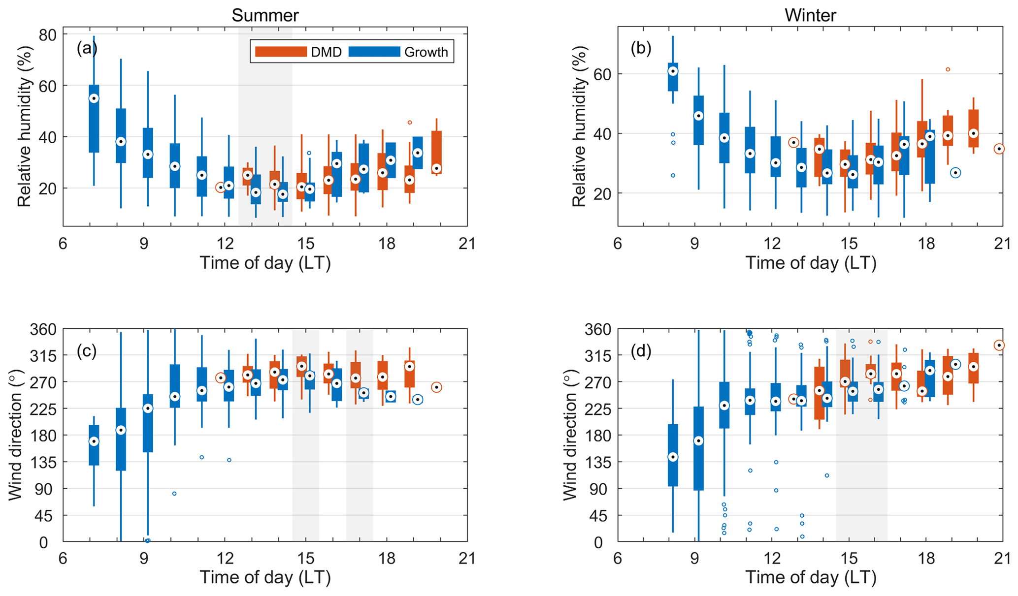
Figure A1Comparison of hourly mean (a, b) relative humidity and (c, d) wind direction between NPF events in the growth phase (blue bars) and DMD phase (orange bars) separately for summer (months: April–September, a, c) and winter (months: October–March, b, d). Statistically significant differences (two-sided Mann–Whitney U test at the 5 % significance level) between the DMD and growth cases are highlighted with grey shading. For each box, the central mark indicates the median, and the bottom and top edges of the box indicate the 25th and 75th percentiles, respectively. The whiskers extend to the most extreme data points not considered outliers, and the outliers (distance from the top or bottom edge of the box more than 1.5 times the interquartile range) are plotted individually using the o symbols.
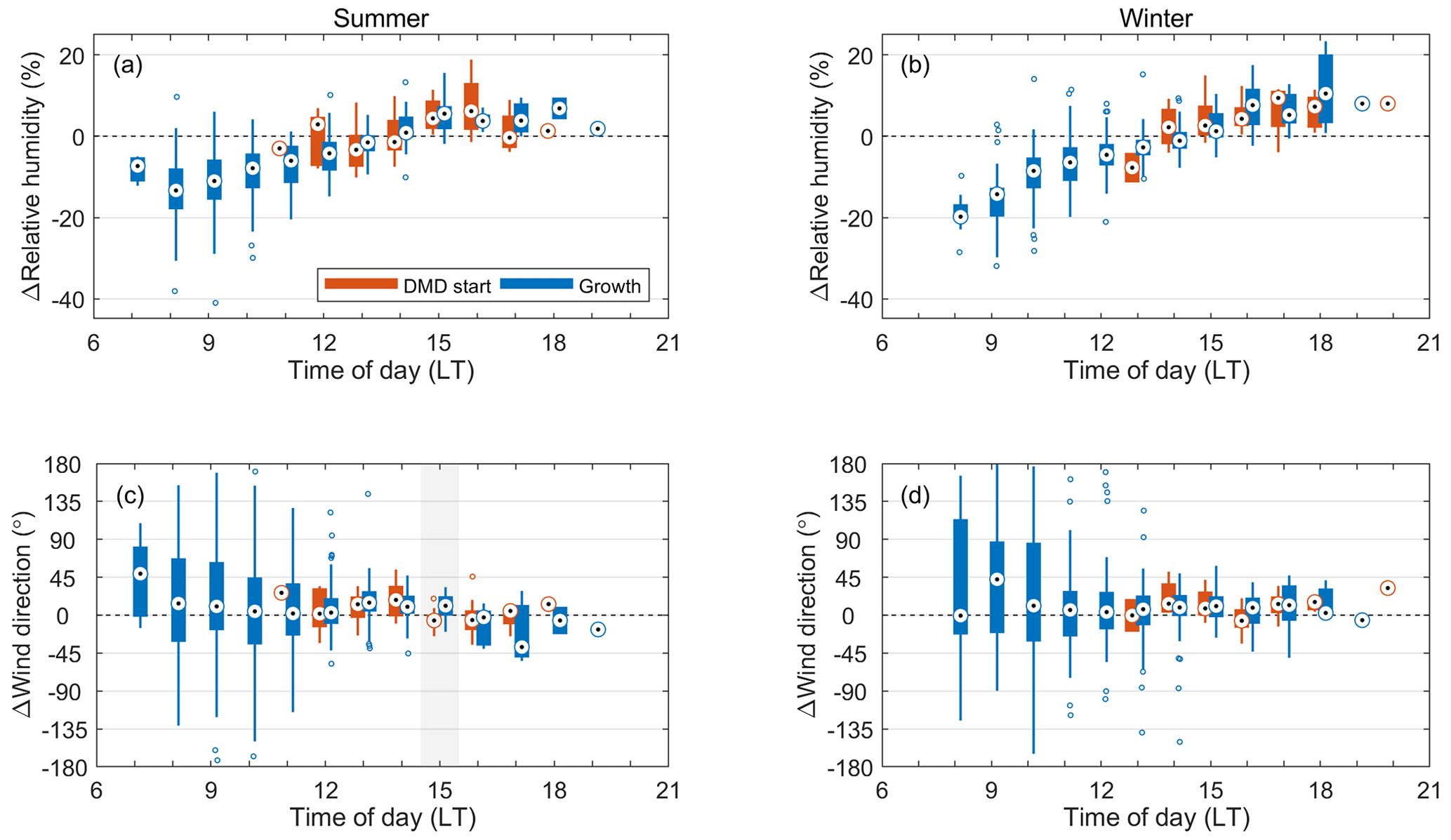
Figure A2Comparison of changes in (a, b) relative humidity and (c, d) wind direction between growth hours (blue bars) and the transition into the DMD phase (orange bars) separately for summer (months: April–September, a, c) and winter (months: October–March, b, d). For variable X the change ΔX at time t is calculated as the difference between the hourly means at t+1 h and t−1 h. Values are included in the DMD start category at time t if the DMD start time is found at t ± 0.5 h. Statistically significant differences (two-sided Mann–Whitney U test at the 5 % significance level) between the DMD start and growth cases are highlighted with grey shading. For each box, the central mark indicates the median, and the bottom and top edges of the box indicate the 25th and 75th percentiles, respectively. The whiskers extend to the most extreme data points not considered outliers, and the outliers (distance from the top or bottom edge of the box more than 1.5 times the interquartile range) are plotted individually using the o symbols.
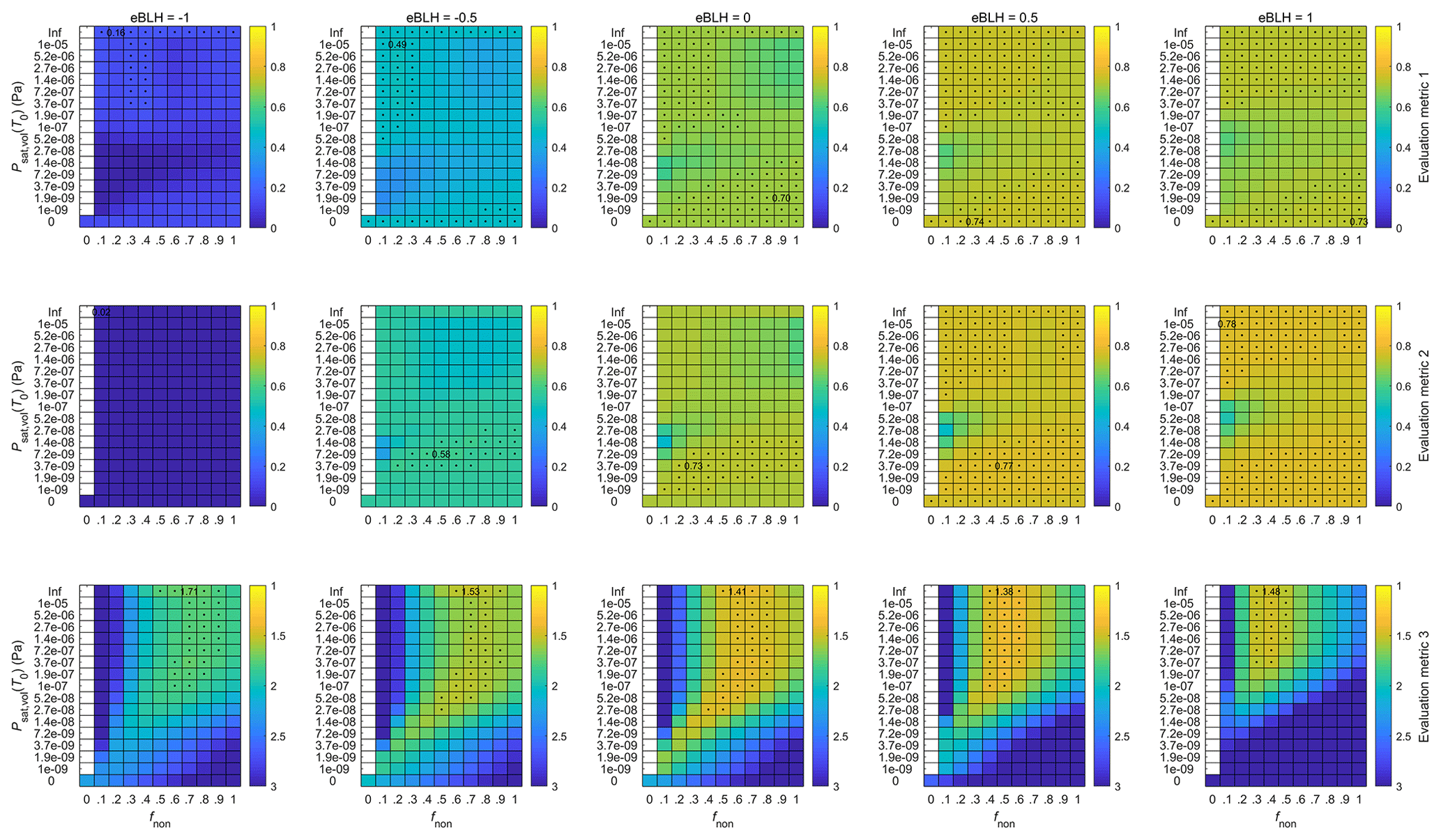
Figure A3Evaluation of the model performance with different exponents for the boundary layer height term (eBLH) when eWS = 0, eCS = 0, fvol = 1 and Δhvol= 80 kJ mol−1. Each column of panels contains the performance matrices of the three different evaluation metrics as a function of the concentration multiplier for the non-volatile compound (fnon) and the saturation vapor pressure of the volatile compound (Psat,vol(T0)) with a specific eBLH value. In the first two rows, higher correlation values of the evaluation metrics indicate better model performance, while in the last row, lower deviations correspond to better results. In each panel, the value of the best model performance is shown in numbers. Values close to the best one (differences of less than 0.015 in the correlation values and less than 5 % in the deviation value) are highlighted with black dots. Each model run, resulting in a single data point for each of the evaluation metrics, comprises 138 NPF event days.
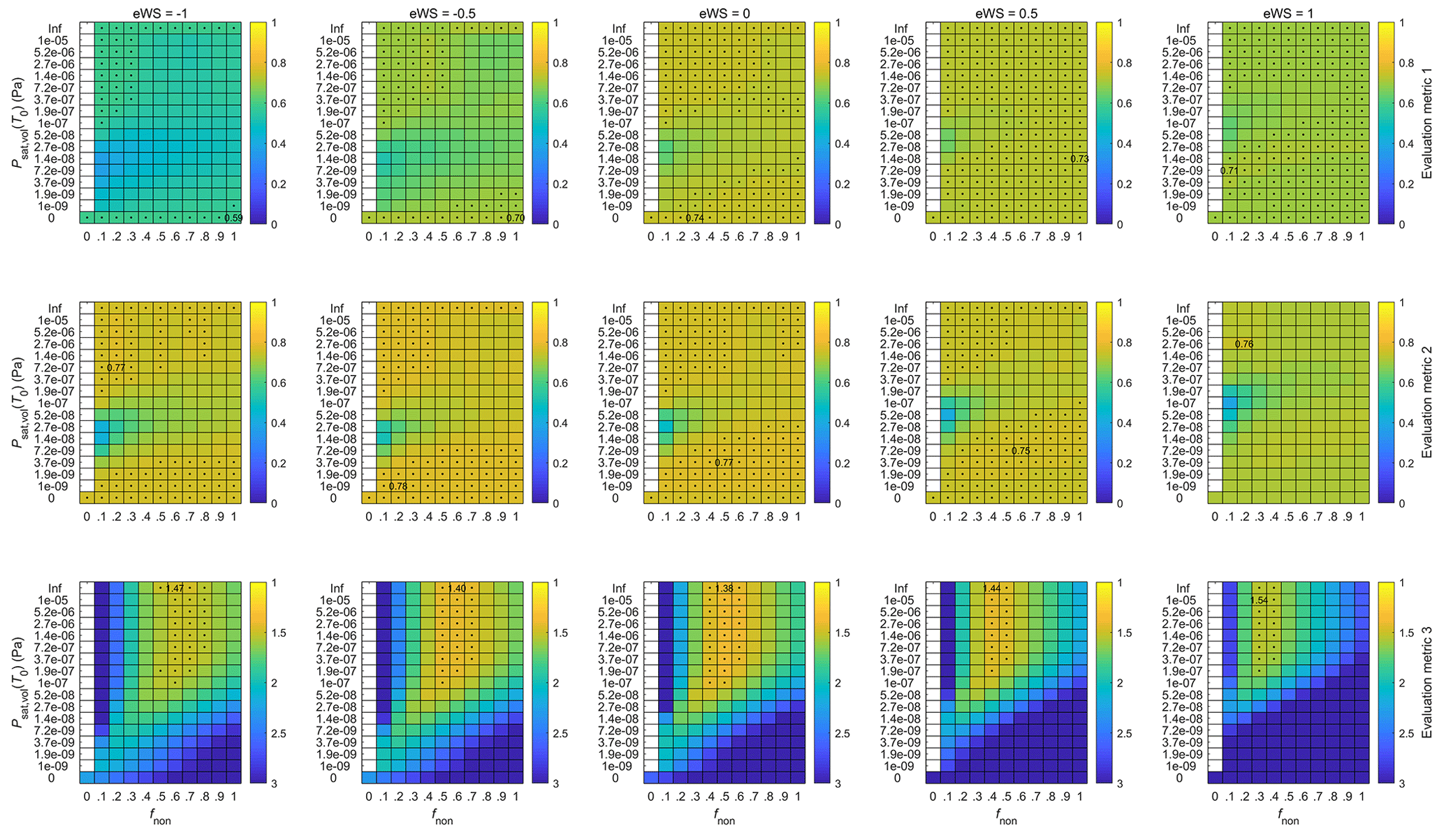
Figure A4Evaluation of the model performance with different exponents for the wind speed term (eWS) when eBLH = 0.5, eCS = 0, fvol= 1 and Δhvol= 80 kJ mol−1. Each column of panels contains the performance matrices of the three different evaluation metrics as a function of the concentration multiplier for the non-volatile compound (fnon) and the saturation vapor pressure of the volatile compound (Psat,vol(T0)) with a specific eWS value. In the first two rows, higher correlation values of the evaluation metrics indicate better model performance, while in the last row, lower deviations correspond to better results. In each panel, the value of the best model performance is shown in numbers. Values close to the best one (differences of less than 0.015 in the correlation values and less than 5 % in the deviation value) are highlighted with black dots. Each model run, resulting in a single data point for each of the evaluation metrics, comprises 138 NPF event days.
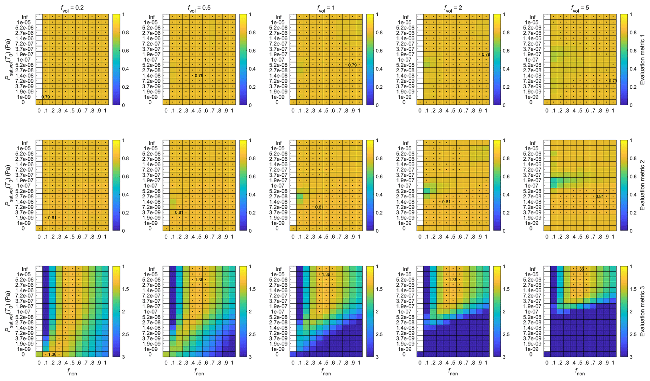
Figure A5Evaluation of the model performance with different concentration multipliers for the volatile component (fvol) when eBLH = 0.5, eWS = 0, eCS = −0.5 and Δhvol= 80 kJ mol−1. Each column of panels contains the performance matrices of the three different evaluation metrics as a function of the concentration multiplier for the non-volatile compound (fnon) and the saturation vapor pressure of the volatile compound (Psat,vol(T0)) with a specific fvol value. In the first two rows, higher correlation values of the evaluation metrics indicate better model performance, while in the last row, lower deviations correspond to better results. In each panel, the value of the best model performance is shown in numbers. Values close to the best one (differences of less than 0.015 in the correlation values and less than 5 % in the deviation value) are highlighted with black dots. Each model run, resulting in a single data point for each of the evaluation metrics, comprises 138 NPF event days.
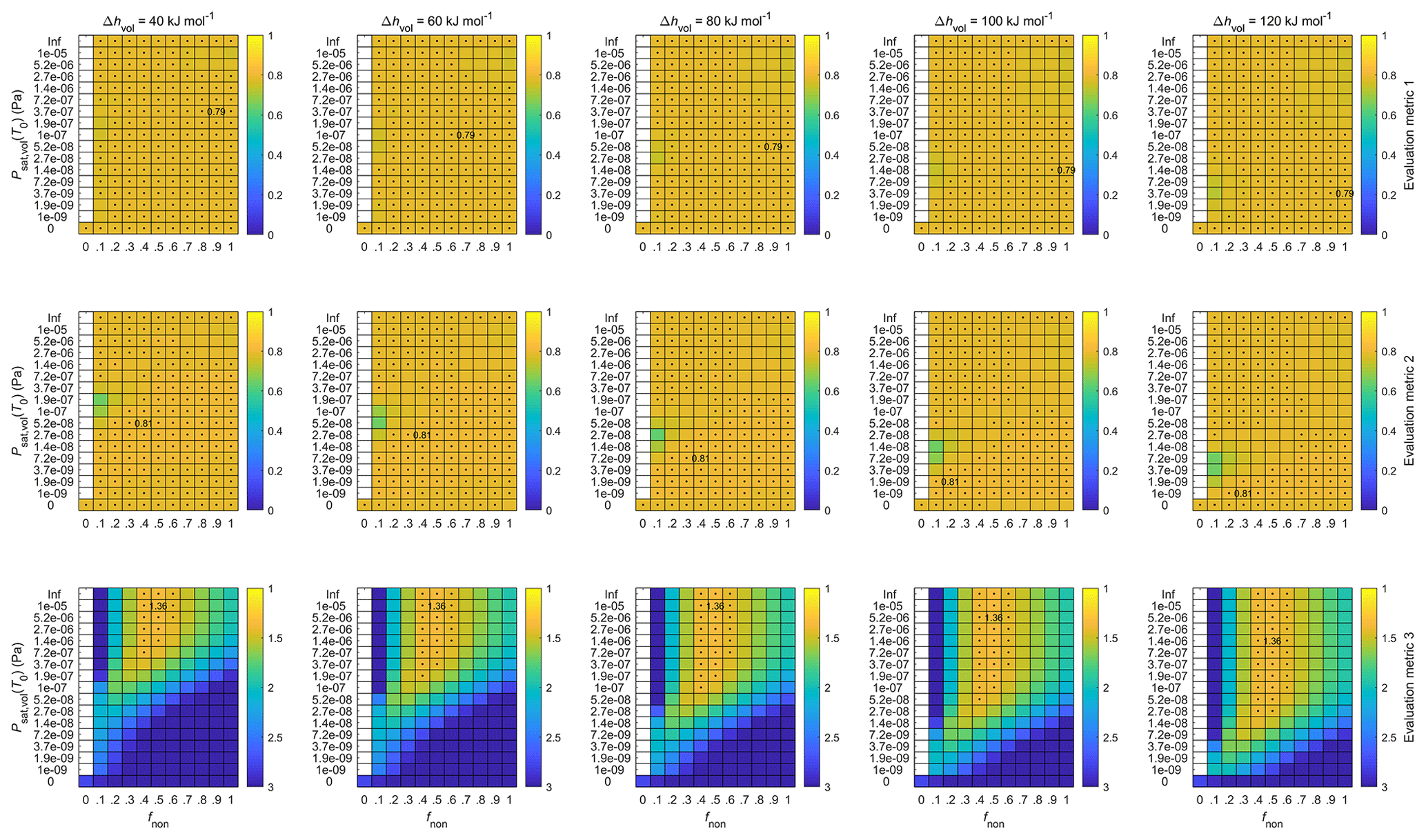
Figure A6Evaluation of the model performance with different enthalpies of vaporization for the volatile component (Δhvol) when eBLH = 0.5, eWS = 0, eCS = −0.5 and fvol= 80 kJ mol−1. Each column of panels contains the performance matrices of the three different evaluation metrics as a function of the concentration multiplier for the non-volatile compound (fnon) and the saturation vapor pressure of the volatile compound (Psat,vol(T0)) with a specific Δhvol value. In the first two rows, higher correlation values of the evaluation metrics indicate better model performance, while in the last row, lower deviations correspond to better results. In each panel, the value of the best model performance is shown in numbers. Values close to the best one (differences of less than 0.015 in the correlation values and less than 5 % in the deviation value) are highlighted with black dots. Each model run, resulting in a single data point for each of the evaluation metrics, comprises 138 NPF event days.
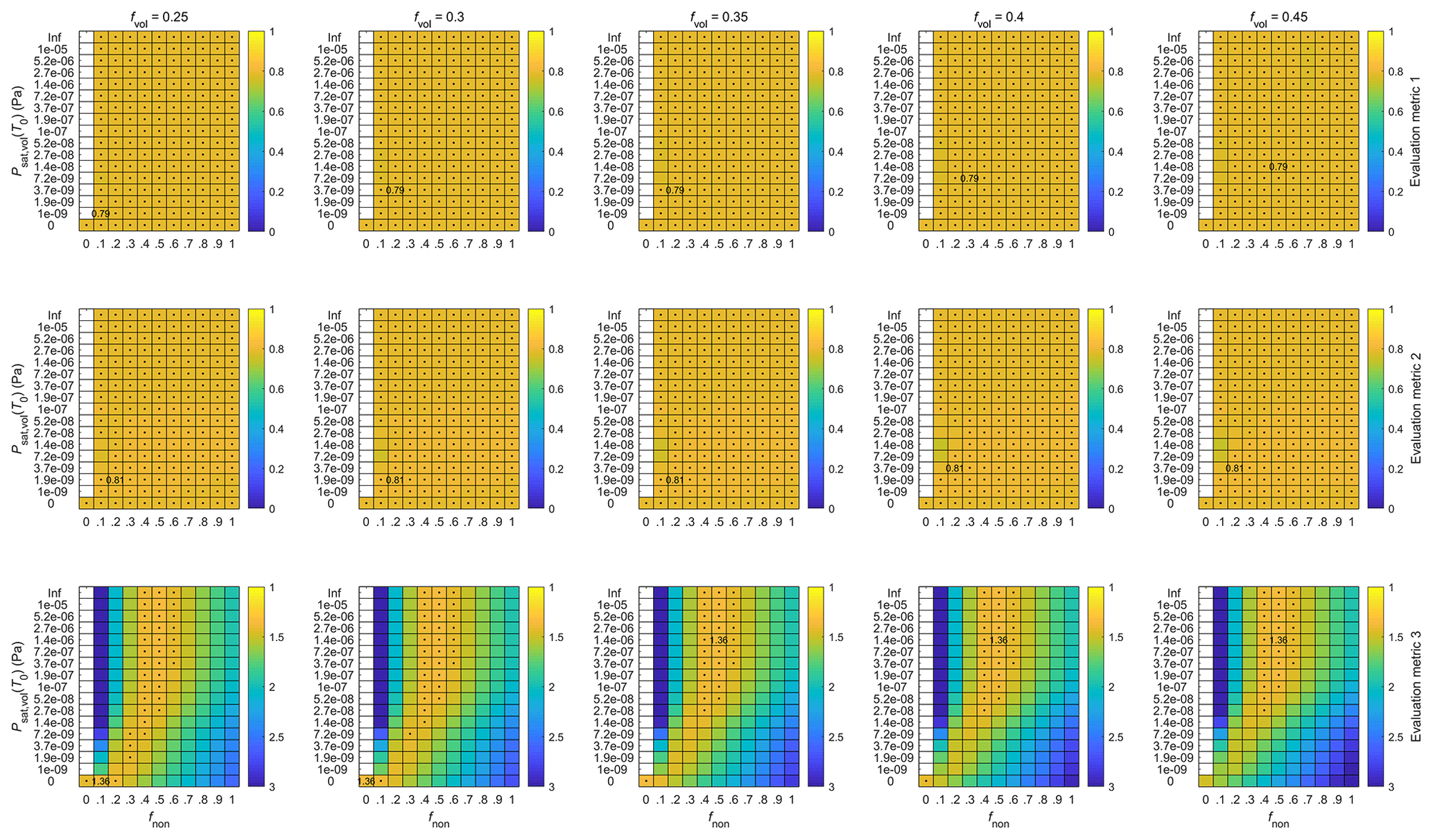
Figure A7Evaluation of the model performance with different concentration multipliers for the volatile component (fvol) in the 0.2–0.5 range when eBLH = 0.5, eWS = 0, eCS = −0.5 and Δhvol= 80 kJ mol−1. Each column of panels contains the performance matrices of the three different evaluation metrics as a function of the concentration multiplier for the non-volatile compound (fnon) and the saturation vapor pressure of the volatile compound (Psat,vol(T0)) with a specific fvol value. In the first two rows, higher correlation values of the evaluation metrics indicate better model performance, while in the last row, lower deviations correspond to better results. In each panel, the value of the best model performance is shown in numbers. Values close to the best one (differences of less than 0.015 in the correlation values and less than 5 % in the deviation value) are highlighted with black dots. Each model run, resulting in a single data point for each of the evaluation metrics, comprises 138 NPF event days.
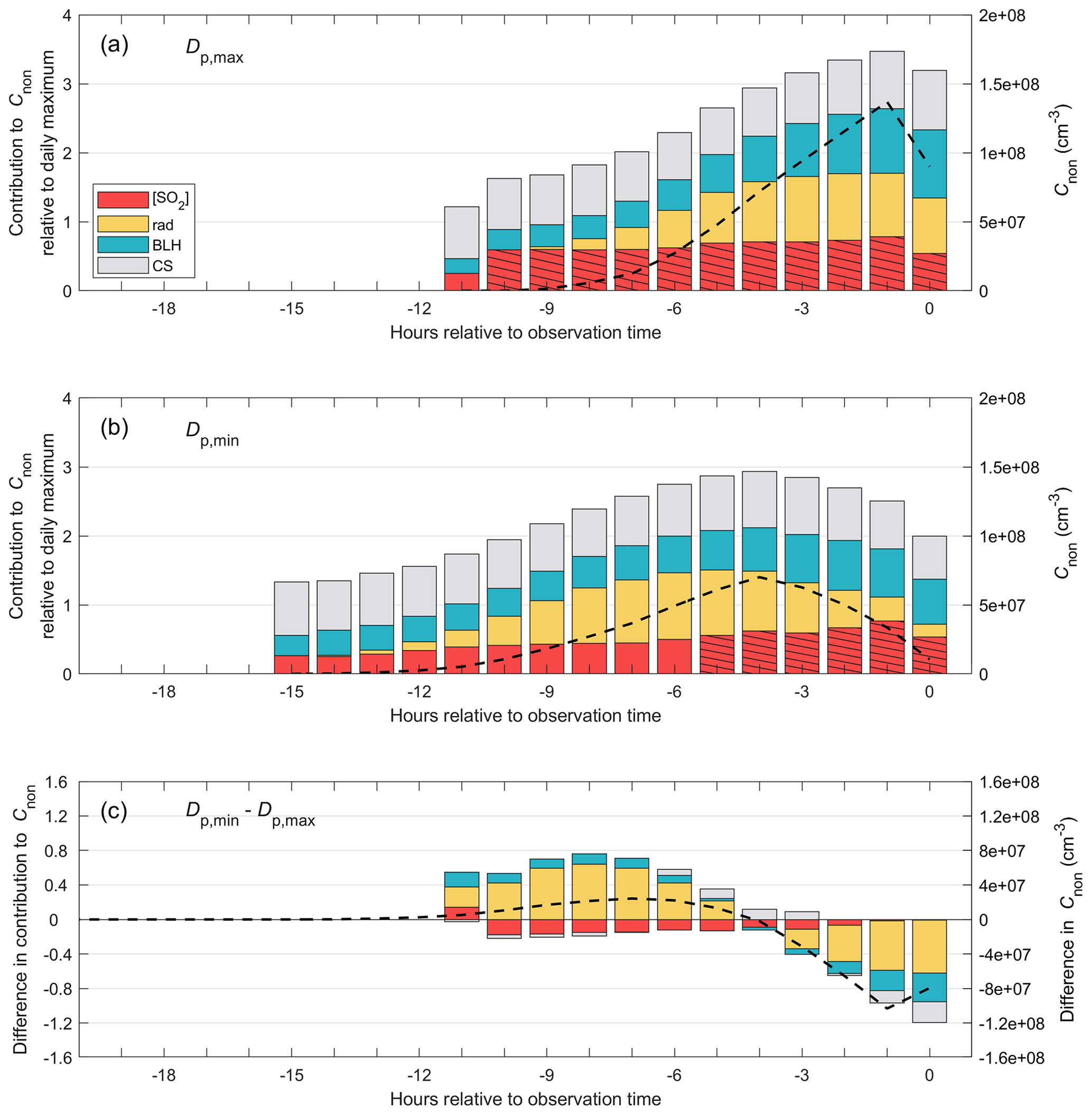
Figure A8Same as Fig. 10 in the main text but with the horizontal axis in hours relative to the observation time of (a) the daily largest modeled particle (Dp,max) and (b) the smallest modeled particle in the evening (Dp,min) instead of the local time.
Data used in this study are available from the corresponding author upon request (simo.hakala@helsinki.fi).
The work was conceptualized by SH and PP. SH was responsible for the methodology, formal analysis, visualization and writing of the original draft. Funding for the work was acquired by SH, MK, TP, TH, MIK, MAA and PP, while the investigation was performed by HL, APH, KN and MIK. HL, APH, TP and TH were responsible for the project administration and PP, MK and VMK supervised the work. VV provided software regarding the computation of the air mass back-trajectories. All the authors contributed to reviewing and editing the manuscript.
At least one of the (co-)authors is a member of the editorial board of Atmospheric Chemistry and Physics. The peer-review process was guided by an independent editor, and the authors also have no other competing interests to declare.
Publisher’s note: Copernicus Publications remains neutral with regard to jurisdictional claims in published maps and institutional affiliations.
The authors wish to thank CSC – IT Center for Science, Finland, for generous computational resources and Anu-Maija Sundström for their contributions towards utilizing the OMI satellite data. Tareq Hussein thanks the Eastern Mediterranean and Middle East Climate and Atmosphere Research (EMME-CARE) project, which received funding from the European Union's Horizon 2020 research and innovation program (grant no. 856612) and the government of Cyprus. The sole responsibility for this publication lies with the authors.
This study was funded by the Deanship of Scientific Research (DSR, grant no. I-122-430) at King Abdulaziz University (KAU), the Academy of Finland (ACCC Flagship, project 337549; Centre of Excellence program, projects 272041 and 307331; Profi 3 program, project 311932; Academy professorship, project 302958; and projects 325656 and 325647), the European Research Council (ERC) under the European Union's Horizon 2020 research and innovation program (ATM-GTP, grant no. 742206; FORCeS, grant no. 821205), the Horizon Europe project FOCI, Non-CO2 Forcers and Their Climate, Weather, Air Quality and Health Impacts (project 101056783) and the Doctoral Programme in Atmospheric Sciences at the University of Helsinki (ATM-DP).
Open-access funding was provided by Helsinki University Library.
This paper was edited by Joachim Curtius and reviewed by two anonymous referees.
Al-Jeelani, H. A.: Diurnal and Seasonal Variations of Surface Ozone and Its Precursors in the Atmosphere of Yanbu, Saudi Arabia, J. Environm. Prot., 5, 408–422, https://doi.org/10.4236/jep.2014.55044, 2014.
Al-Jeelani, H. A.: Evaluation of air quality in the Holy Makkah during Hajj season 1425 H, Journal of Applied Sciences Research, 5, 115–121, 2009.
Alghamdi, M. A., Khoder, M., Abdelmaksoud, A. S., Harrison, R. M., Hussein, T., Lihavainen, H., Al-Jeelani, H., Goknil, M. H., Shabbaj, I. I., Almehmadi, F. M., Hyvärinen, A. P., and Hämeri, K.: Seasonal and diurnal variations of BTEX and their potential for ozone formation in the urban background atmosphere of the coastal city Jeddah, Saudi Arabia, Air Qual. Atmos. Hlth., 7, 467–480, https://doi.org/10.1007/s11869-014-0263-x, 2014.
Alonso-Blanco, E., Gómez-Moreno, F. J., Núñez, L., Pujadas, M., Cusack, M., and Artíñano, B.: Aerosol particle shrinkage event phenomenology in a South European suburban area during 2009–2015, Atmos. Environ., 160, 154–164, doi”10.1016/j.atmosenv.2017.04.013, 2017.
Backman, J., Rizzo, L. V., Hakala, J., Nieminen, T., Manninen, H. E., Morais, F., Aalto, P. P., Siivola, E., Carbone, S., Hillamo, R., Artaxo, P., Virkkula, A., Petäjä, T., and Kulmala, M.: On the diurnal cycle of urban aerosols, black carbon and the occurrence of new particle formation events in springtime São Paulo, Brazil, Atmos. Chem. Phys., 12, 11733–11751, https://doi.org/10.5194/acp-12-11733-2012, 2012.
Baltensperger, U., Kalberer, M., Dommen, J., Paulsen, D., Alfarra, M. R., Coe, H., Fisseha, R., Gascho, A., Gysel, M., Nyeki, S., Sax, M., Steinbacher, M., Prevot, A. S. H., Sjögren, S., Weingartner, E., and Zenobi, R.: Secondary organic aerosols from anthropogenic and biogenic precursors, Faraday Discuss., 130, 265–278, https://doi.org/10.1039/B417367H, 2005.
Bourtsoukidis, E., Ernle, L., Crowley, J. N., Lelieveld, J., Paris, J.-D., Pozzer, A., Walter, D., and Williams, J.: Non-methane hydrocarbon (C2–C8) sources and sinks around the Arabian Peninsula, Atmos. Chem. Phys., 19, 7209–7232, https://doi.org/10.5194/acp-19-7209-2019, 2019.
Cai, R., Yin, R., Yan, C., Yang, D., Deng, C., Dada, L., Kangasluoma, J., Kontkanen, J., Halonen, R., Ma, Y., Zhang, X., Paasonen, P., Petäjä, T., Kerminen, V.-M., Liu, Y., Bianchi, F., Zheng, J., Wang, L., Hao, J., Smith, J. N., Donahue, N. M., Kulmala, M., Worsnop, D. R., and Jiang, J.: The missing base molecules in atmospheric acid–base nucleation, Natl. Sci. Rev., 9, nwac137, https://doi.org/10.1093/nsr/nwac137, 2022.
Cusack, M., Alastuey, A., and Querol, X.: Case studies of new particle formation and evaporation processes in the western Mediterranean regional background, Atmos. Environ., 81, 651–659, https://doi.org/10.1016/j.atmosenv.2013.09.025, 2013.
Dada, L., Ylivinkka, I., Baalbaki, R., Li, C., Guo, Y., Yan, C., Yao, L., Sarnela, N., Jokinen, T., Daellenbach, K. R., Yin, R., Deng, C., Chu, B., Nieminen, T., Wang, Y., Lin, Z., Thakur, R. C., Kontkanen, J., Stolzenburg, D., Sipilä, M., Hussein, T., Paasonen, P., Bianchi, F., Salma, I., Weidinger, T., Pikridas, M., Sciare, J., Jiang, J., Liu, Y., Petäjä, T., Kerminen, V.-M., and Kulmala, M.: Sources and sinks driving sulfuric acid concentrations in contrasting environments: implications on proxy calculations, Atmos. Chem. Phys., 20, 11747–11766, https://doi.org/10.5194/acp-20-11747-2020, 2020.
Dal Maso, M., Kulmala, M., Riipinen, I., Wagner, R., Hussein, T., Aalto, P. P., and Lehtinen, K. E. J.: Formation and growth of fresh atmospheric aerosols: eight years of aerosol size distribution data from SMEAR II, Hyytiälä, Finland, Boreal Environ. Res., 10, 323–336, 2005.
Dall'Osto, M., Beddows, D. C. S., Asmi, A., Poulain, L., Hao, L., Freney, E., Allan, J. D., Canagaratna, M., Crippa, M., Bianchi, F., de Leeuw, G., Eriksson, A., Swietlicki, E., Hansson, H. C., Henzing, J. S., Granier, C., Zemankova, K., Laj, P., Onasch, T., Prevot, A., Putaud, J. P., Sellegri, K., Vidal, M., Virtanen, A., Simo, R., Worsnop, D., O'Dowd, C., Kulmala, M., and Harrison, R. M.: Novel insights on new particle formation derived from a pan-european observing system, Sci. Rep.-UK, 8, 1482, https://doi.org/10.1038/s41598-017-17343-9, 2018.
De Smedt, I., Pinardi, G., Vigouroux, C., Compernolle, S., Bais, A., Benavent, N., Boersma, F., Chan, K.-L., Donner, S., Eichmann, K.-U., Hedelt, P., Hendrick, F., Irie, H., Kumar, V., Lambert, J.-C., Langerock, B., Lerot, C., Liu, C., Loyola, D., Piters, A., Richter, A., Rivera Cárdenas, C., Romahn, F., Ryan, R. G., Sinha, V., Theys, N., Vlietinck, J., Wagner, T., Wang, T., Yu, H., and Van Roozendael, M.: Comparative assessment of TROPOMI and OMI formaldehyde observations and validation against MAX-DOAS network column measurements, Atmos. Chem. Phys., 21, 12561–12593, https://doi.org/10.5194/acp-21-12561-2021, 2021.
Donahue, N. M., Kroll, J. H., Pandis, S. N., and Robinson, A. L.: A two-dimensional volatility basis set – Part 2: Diagnostics of organic-aerosol evolution, Atmos. Chem. Phys., 12, 615–634, https://doi.org/10.5194/acp-12-615-2012, 2012.
Ehn, M., Thornton, J. A., Kleist, E., Sipila, M., Junninen, H., Pullinen, I., Springer, M., Rubach, F., Tillmann, R., Lee, B., Lopez-Hilfiker, F., Andres, S., Acir, I. H., Rissanen, M., Jokinen, T., Schobesberger, S., Kangasluoma, J., Kontkanen, J., Nieminen, T., Kurten, T., Nielsen, L. B., Jorgensen, S., Kjaergaard, H. G., Canagaratna, M., Dal Maso, M., Berndt, T., Petaja, T., Wahner, A., Kerminen, V. M., Kulmala, M., Worsnop, D. R., Wildt, J., and Mentel, T. F.: A large source of low-volatility secondary organic aerosol, Nature, 506, 476–479, https://doi.org/10.1038/nature13032, 2014.
Gordon, H., Kirkby, J., Baltensperger, U., Bianchi, F., Breitenlechner, M., Curtius, J., Dias, A., Dommen, J., Donahue, N. M., Dunne, E. M., Duplissy, J., Ehrhart, S., Flagan, R. C., Frege, C., Fuchs, C., Hansel, A., Hoyle, C. R., Kulmala, M., Kurten, A., Lehtipalo, K., Makhmutov, V., Molteni, U., Rissanen, M. P., Stozkhov, Y., Trostl, J., Tsagkogeorgas, G., Wagner, R., Williamson, C., Wimmer, D., Winkler, P. M., Yan, C., and Carslaw, K. S.: Causes and importance of new particle formation in the present-day and preindustrial atmospheres, J. Geophys. Res.-Atmos., 122, 8739–8760, https://doi.org/10.1002/2017jd026844, 2017.
Guo, H., Wang, D. W., Cheung, K., Ling, Z. H., Chan, C. K., and Yao, X. H.: Observation of aerosol size distribution and new particle formation at a mountain site in subtropical Hong Kong, Atmos. Chem. Phys., 12, 9923–9939, https://doi.org/10.5194/acp-12-9923-2012, 2012.
Hakala, S., Alghamdi, M. A., Paasonen, P., Vakkari, V., Khoder, M. I., Neitola, K., Dada, L., Abdelmaksoud, A. S., Al-Jeelani, H., Shabbaj, I. I., Almehmadi, F. M., Sundström, A.-M., Lihavainen, H., Kerminen, V.-M., Kontkanen, J., Kulmala, M., Hussein, T., and Hyvärinen, A.-P.: New particle formation, growth and apparent shrinkage at a rural background site in western Saudi Arabia, Atmos. Chem. Phys., 19, 10537–10555, https://doi.org/10.5194/acp-19-10537-2019, 2019.
Häkkinen, E., Zhao, J., Graeffe, F., Fauré, N., Krechmer, J. E., Worsnop, D., Timonen, H., Ehn, M., and Kangasluoma, J.: Online measurement of highly oxygenated compounds from organic aerosol, Atmos. Meas. Tech., 16, 1705–1721, https://doi.org/10.5194/amt-16-1705-2023, 2023.
Henze, D. K., Seinfeld, J. H., Ng, N. L., Kroll, J. H., Fu, T.-M., Jacob, D. J., and Heald, C. L.: Global modeling of secondary organic aerosol formation from aromatic hydrocarbons: high- vs. low-yield pathways, Atmos. Chem. Phys., 8, 2405–2420, https://doi.org/10.5194/acp-8-2405-2008, 2008.
Hong, J., Äijälä, M., Häme, S. A. K., Hao, L., Duplissy, J., Heikkinen, L. M., Nie, W., Mikkilä, J., Kulmala, M., Prisle, N. L., Virtanen, A., Ehn, M., Paasonen, P., Worsnop, D. R., Riipinen, I., Petäjä, T., and Kerminen, V.-M.: Estimates of the organic aerosol volatility in a boreal forest using two independent methods, Atmos. Chem. Phys., 17, 4387–4399, https://doi.org/10.5194/acp-17-4387-2017, 2017.
Huang, X., Zhou, L., Ding, A., Qi, X., Nie, W., Wang, M., Chi, X., Petäjä, T., Kerminen, V.-M., Roldin, P., Rusanen, A., Kulmala, M., and Boy, M.: Comprehensive modelling study on observed new particle formation at the SORPES station in Nanjing, China, Atmos. Chem. Phys., 16, 2477–2492, https://doi.org/10.5194/acp-16-2477-2016, 2016.
Huffman, J. A., Docherty, K. S., Aiken, A. C., Cubison, M. J., Ulbrich, I. M., DeCarlo, P. F., Sueper, D., Jayne, J. T., Worsnop, D. R., Ziemann, P. J., and Jimenez, J. L.: Chemically-resolved aerosol volatility measurements from two megacity field studies, Atmos. Chem. Phys., 9, 7161–7182, https://doi.org/10.5194/acp-9-7161-2009, 2009.
Hussein, T., Dal Maso, M., Petaja, T., Koponen, I. K., Paatero, P., Aalto, P. P., Hameri, K., and Kulmala, M.: Evaluation of an automatic algorithm for fitting the particle number size distributions, Boreal Environ. Res., 10, 337–355, 2005.
Hussein, T., Junninen, H., Tunved, P., Kristensson, A., Dal Maso, M., Riipinen, I., Aalto, P. P., Hansson, H.-C., Swietlicki, E., and Kulmala, M.: Time span and spatial scale of regional new particle formation events over Finland and Southern Sweden, Atmos. Chem. Phys., 9, 4699–4716, https://doi.org/10.5194/acp-9-4699-2009, 2009.
IPCC: Climate Change 2021: The Physical Science Basis. Contribution of Working Group I to the Sixth Assessment Report of the Intergovernmental Panel on Climate Change, edited by: Masson-Delmotte, V., Zhai, P., Pirani, A., Connors, S. L., Péan, C., Berger, S., Caud, N., Chen, Y., Goldfarb, L., Gomis, M. I., Huang, M., Leitzell, K., Lonnoy, E., Matthews, J. B. R., Maycock, T. K., Waterfield, T., Yelekçi, O., Yu, R., and Zho, B., Cambridge University Press, Cambridge, United Kingdom and New York, NY, USA, 2391 pp., https://doi.org/10.1017/9781009157896, 2021.
Jimenez, J. L., Canagaratna, M. R., Donahue, N. M., Prevot, A. S. H., Zhang, Q., Kroll, J. H., DeCarlo, P. F., Allan, J. D., Coe, H., Ng, N. L., Aiken, A. C., Docherty, K. S., Ulbrich, I. M., Grieshop, A. P., Robinson, A. L., Duplissy, J., Smith, J. D., Wilson, K. R., Lanz, V. A., Hueglin, C., Sun, Y. L., Tian, J., Laaksonen, A., Raatikainen, T., Rautiainen, J., Vaattovaara, P., Ehn, M., Kulmala, M., Tomlinson, J. M., Collins, D. R., Cubison, M. J., null, n., Dunlea, J., Huffman, J. A., Onasch, T. B., Alfarra, M. R., Williams, P. I., Bower, K., Kondo, Y., Schneider, J., Drewnick, F., Borrmann, S., Weimer, S., Demerjian, K., Salcedo, D., Cottrell, L., Griffin, R., Takami, A., Miyoshi, T., Hatakeyama, S., Shimono, A., Sun, J. Y., Zhang, Y. M., Dzepina, K., Kimmel, J. R., Sueper, D., Jayne, J. T., Herndon, S. C., Trimborn, A. M., Williams, L. R., Wood, E. C., Middlebrook, A. M., Kolb, C. E., Baltensperger, U., and Worsnop, D. R.: Evolution of Organic Aerosols in the Atmosphere, Science, 326, 1525–1529, https://doi.org/10.1126/science.1180353, 2009.
Kerminen, V.-M., Paramonov, M., Anttila, T., Riipinen, I., Fountoukis, C., Korhonen, H., Asmi, E., Laakso, L., Lihavainen, H., Swietlicki, E., Svenningsson, B., Asmi, A., Pandis, S. N., Kulmala, M., and Petäjä, T.: Cloud condensation nuclei production associated with atmospheric nucleation: a synthesis based on existing literature and new results, Atmos. Chem. Phys., 12, 12037–12059, https://doi.org/10.5194/acp-12-12037-2012, 2012.
Kerminen, V. M., Chen, X., Vakkari, V., Petäjä, T., Kulmala, M., and Bianchi, F.: Atmospheric new particle formation and growth: review of field observations, Environ. Res. Lett., 13, 103003, https://doi.org/10.1088/1748-9326/aadf3c, 2018.
Kesti, J., Backman, J., O'Connor, E. J., Hirsikko, A., Asmi, E., Aurela, M., Makkonen, U., Filioglou, M., Komppula, M., Korhonen, H., and Lihavainen, H.: Aerosol particle characteristics measured in the United Arab Emirates and their response to mixing in the boundary layer, Atmos. Chem. Phys., 22, 481–503, https://doi.org/10.5194/acp-22-481-2022, 2022.
Khodeir, M., Shamy, M., Alghamdi, M., Zhong, M., Sun, H., Costa, M., Chen, L.-C., and Maciejczyk, P.: Source apportionment and elemental composition of PM2.5 and PM10 in Jeddah City, Saudi Arabia, Atmos. Pollut. Res., 3, 331–340, https://doi.org/10.5094/APR.2012.037, 2012.
Kivekäs, N., Carpman, J., Roldin, P., Leppa, J., O'Connor, E., Kristensson, A., and Asmi, E.: Coupling an aerosol box model with one-dimensional flow: a tool for understanding observations of new particle formation events, Tellus B, 68, 29706, https://doi.org/10.3402/tellusb.v68.29706, 2016.
Kontkanen, J., Paasonen, P., Aalto, J., Bäck, J., Rantala, P., Petäjä, T., and Kulmala, M.: Simple proxies for estimating the concentrations of monoterpenes and their oxidation products at a boreal forest site, Atmos. Chem. Phys., 16, 13291–13307, https://doi.org/10.5194/acp-16-13291-2016, 2016.
Krechmer, J. E., Coggon, M. M., Massoli, P., Nguyen, T. B., Crounse, J. D., Hu, W., Day, D. A., Tyndall, G. S., Henze, D. K., Rivera-Rios, J. C., Nowak, J. B., Kimmel, J. R., Mauldin III, R. L., Stark, H., Jayne, J. T., Sipilä, M., Junninen, H., St. Clair, J. M., Zhang, X., Feiner, P. A., Zhang, L., Miller, D. O., Brune, W. H., Keutsch, F. N., Wennberg, P. O., Seinfeld, J. H., Worsnop, D. R., Jimenez, J. L., and Canagaratna, M. R.: Formation of Low Volatility Organic Compounds and Secondary Organic Aerosol from Isoprene Hydroxyhydroperoxide Low-NO Oxidation, Environ. Sci. Technol., 49, 10330–10339, https://doi.org/10.1021/acs.est.5b02031, 2015.
Krotkov, N. A., McLinden, C. A., Li, C., Lamsal, L. N., Celarier, E. A., Marchenko, S. V., Swartz, W. H., Bucsela, E. J., Joiner, J., Duncan, B. N., Boersma, K. F., Veefkind, J. P., Levelt, P. F., Fioletov, V. E., Dickerson, R. R., He, H., Lu, Z., and Streets, D. G.: Aura OMI observations of regional SO2 and NO2 pollution changes from 2005 to 2015, Atmos. Chem. Phys., 16, 4605–4629, https://doi.org/10.5194/acp-16-4605-2016, 2016.
Kürten, A., Li, C., Bianchi, F., Curtius, J., Dias, A., Donahue, N. M., Duplissy, J., Flagan, R. C., Hakala, J., Jokinen, T., Kirkby, J., Kulmala, M., Laaksonen, A., Lehtipalo, K., Makhmutov, V., Onnela, A., Rissanen, M. P., Simon, M., Sipilä, M., Stozhkov, Y., Tröstl, J., Ye, P., and McMurry, P. H.: New particle formation in the sulfuric acid–dimethylamine–water system: reevaluation of CLOUD chamber measurements and comparison to an aerosol nucleation and growth model, Atmos. Chem. Phys., 18, 845–863, https://doi.org/10.5194/acp-18-845-2018, 2018.
Laaksonen, A., Kulmala, M., O'Dowd, C. D., Joutsensaari, J., Vaattovaara, P., Mikkonen, S., Lehtinen, K. E. J., Sogacheva, L., Dal Maso, M., Aalto, P., Petäjä, T., Sogachev, A., Yoon, Y. J., Lihavainen, H., Nilsson, D., Facchini, M. C., Cavalli, F., Fuzzi, S., Hoffmann, T., Arnold, F., Hanke, M., Sellegri, K., Umann, B., Junkermann, W., Coe, H., Allan, J. D., Alfarra, M. R., Worsnop, D. R., Riekkola, M.-L., Hyötyläinen, T., and Viisanen, Y.: The role of VOC oxidation products in continental new particle formation, Atmos. Chem. Phys., 8, 2657–2665, https://doi.org/10.5194/acp-8-2657-2008, 2008.
Lai, S., Hai, S., Gao, Y., Wang, Y., Sheng, L., Lupascu, A., Ding, A., Nie, W., Qi, X., Huang, X., Chi, X., Zhao, C., Zhao, B., Shrivastava, M., Fast, J. D., Yao, X., and Gao, H.: The striking effect of vertical mixing in the planetary boundary layer on new particle formation in the Yangtze River Delta, Sci. Total Environ., 829, 154607, https://doi.org/10.1016/j.scitotenv.2022.154607, 2022a.
Lai, S., Huang, X., Qi, X., Chen, L., Ren, C., Wang, Z., Wang, J., Lou, S., Chi, X., Gao, Y., Hai, S., Petäjä, T., Kerminen, V.-M., Kulmala, M., and Ding, A.: Vigorous New Particle Formation Above Polluted Boundary Layer in the North China Plain, Geophys. Res. Lett., 49, e2022GL100301, https://doi.org/10.1029/2022GL100301, 2022b.
Levelt, P. F., Van den Oord, G. H. J., Dobber, M. R., Malkki, A., Visser, H., de Vries, J., Stammes, P., Lundell, J. O. V., and Saari, H.: The Ozone Monitoring Instrument, IEEE T. Geosci. Remote, 44, 1093–1101, https://doi.org/10.1109/Tgrs.2006.872333, 2006.
Li, C., Joiner, J., Krotkov, N. A., and Bhartia, P. K.: A fast and sensitive new satellite SO2 retrieval algorithm based on principal component analysis: Application to the ozone monitoring instrument, Geophys. Res. Lett., 40, 6314–6318, https://doi.org/10.1002/2013gl058134, 2013.
Lihavainen, H., Alghamdi, M. A., Hyvarinen, A. P., Hussein, T., Aaltonen, V., Abdelmaksoud, A. S., Al-Jeelani, H., Almazroui, M., Almehmadi, F. M., Al Zawad, F. M., Hakala, J., Khoder, M., Neitola, K., Petaja, T., Shabbaj, I. I., and Hameri, K.: Aerosols physical properties at Hada Al Sham, western Saudi Arabia, Atmos. Environ., 135, 109–117, https://doi.org/10.1016/j.atmosenv.2016.04.001, 2016.
Liu, F., Choi, S., Li, C., Fioletov, V. E., McLinden, C. A., Joiner, J., Krotkov, N. A., Bian, H., Janssens-Maenhout, G., Darmenov, A. S., and da Silva, A. M.: A new global anthropogenic SO2 emission inventory for the last decade: a mosaic of satellite-derived and bottom-up emissions, Atmos. Chem. Phys., 18, 16571–16586, https://doi.org/10.5194/acp-18-16571-2018, 2018.
Liu, M. and Matsui, H.: Secondary Organic Aerosol Formation Regulates Cloud Condensation Nuclei in the Global Remote Troposphere, Geophys. Res. Lett., 49, e2022GL100543, https://doi.org/10.1029/2022GL100543, 2022.
Merikanto, J., Spracklen, D. V., Mann, G. W., Pickering, S. J., and Carslaw, K. S.: Impact of nucleation on global CCN, Atmos. Chem. Phys., 9, 8601–8616, https://doi.org/10.5194/acp-9-8601-2009, 2009.
Mikkonen, S., Romakkaniemi, S., Smith, J. N., Korhonen, H., Petäjä, T., Plass-Duelmer, C., Boy, M., McMurry, P. H., Lehtinen, K. E. J., Joutsensaari, J., Hamed, A., Mauldin III, R. L., Birmili, W., Spindler, G., Arnold, F., Kulmala, M., and Laaksonen, A.: A statistical proxy for sulphuric acid concentration, Atmos. Chem. Phys., 11, 11319–11334, https://doi.org/10.5194/acp-11-11319-2011, 2011.
Munir, S., Habeebullah, T. M., Seroji, A. R., Morsy, E. A., Mohammed, A. M. F., Saud, W. A., Abdou, A. E. A., and Awad, A. H.: Modeling Particulate Matter Concentrations in Makkah, Applying a Statistical Modeling Approach, Aerosol Air Qual. Res., 13, 901–910, https://doi.org/10.4209/aaqr.2012.11.0314, 2013.
Nieminen, T., Lehtinen, K. E. J., and Kulmala, M.: Sub-10 nm particle growth by vapor condensation – effects of vapor molecule size and particle thermal speed, Atmos. Chem. Phys., 10, 9773–9779, https://doi.org/10.5194/acp-10-9773-2010, 2010.
Nieminen, T., Kerminen, V.-M., Petäjä, T., Aalto, P. P., Arshinov, M., Asmi, E., Baltensperger, U., Beddows, D. C. S., Beukes, J. P., Collins, D., Ding, A., Harrison, R. M., Henzing, B., Hooda, R., Hu, M., Hõrrak, U., Kivekäs, N., Komsaare, K., Krejci, R., Kristensson, A., Laakso, L., Laaksonen, A., Leaitch, W. R., Lihavainen, H., Mihalopoulos, N., Németh, Z., Nie, W., O'Dowd, C., Salma, I., Sellegri, K., Svenningsson, B., Swietlicki, E., Tunved, P., Ulevicius, V., Vakkari, V., Vana, M., Wiedensohler, A., Wu, Z., Virtanen, A., and Kulmala, M.: Global analysis of continental boundary layer new particle formation based on long-term measurements, Atmos. Chem. Phys., 18, 14737–14756, https://doi.org/10.5194/acp-18-14737-2018, 2018.
Olenius, T., Pichelstorfer, L., Stolzenburg, D., Winkler, P. M., Lehtinen, K. E. J., and Riipinen, I.: Robust metric for quantifying the importance of stochastic effects on nanoparticle growth, Sci. Rep.-UK, 8, 14160, https://doi.org/10.1038/s41598-018-32610-z, 2018.
Osipov, S., Chowdhury, S., Crowley, J. N., Tadic, I., Drewnick, F., Borrmann, S., Eger, P., Fachinger, F., Fischer, H., Predybaylo, E., Fnais, M., Harder, H., Pikridas, M., Vouterakos, P., Pozzer, A., Sciare, J., Ukhov, A., Stenchikov, G. L., Williams, J., and Lelieveld, J.: Severe atmospheric pollution in the Middle East is attributable to anthropogenic sources, Commun. Earth Environ., 3, 203, https://doi.org/10.1038/s43247-022-00514-6, 2022.
Paasonen, P., Asmi, A., Petäjä, T., Kajos, M. K., Äijälä, M., Junninen, H., Holst, T., Abbatt, J. P. D., Arneth, A., Birmili, W., van der Gon, H. D., Hamed, A., Hoffer, A., Laakso, L., Laaksonen, A., Richard Leaitch, W., Plass-Dülmer, C., Pryor, S. C., Räisänen, P., Swietlicki, E., Wiedensohler, A., Worsnop, D. R., Kerminen, V.-M., and Kulmala, M.: Warming-induced increase in aerosol number concentration likely to moderate climate change, Nat. Geosci., 6, 438–442, https://doi.org/10.1038/ngeo1800, 2013.
Paasonen, P., Peltola, M., Kontkanen, J., Junninen, H., Kerminen, V.-M., and Kulmala, M.: Comprehensive analysis of particle growth rates from nucleation mode to cloud condensation nuclei in boreal forest, Atmos. Chem. Phys., 18, 12085–12103, https://doi.org/10.5194/acp-18-12085-2018, 2018.
Parajuli, S. P., Stenchikov, G. L., Ukhov, A., Shevchenko, I., Dubovik, O., and Lopatin, A.: Aerosol vertical distribution and interactions with land/sea breezes over the eastern coast of the Red Sea from lidar data and high-resolution WRF-Chem simulations, Atmos. Chem. Phys., 20, 16089–16116, https://doi.org/10.5194/acp-20-16089-2020, 2020.
Petäjä, T., Mauldin, III, R. L., Kosciuch, E., McGrath, J., Nieminen, T., Paasonen, P., Boy, M., Adamov, A., Kotiaho, T., and Kulmala, M.: Sulfuric acid and OH concentrations in a boreal forest site, Atmos. Chem. Phys., 9, 7435–7448, https://doi.org/10.5194/acp-9-7435-2009, 2009.
Pisso, I., Sollum, E., Grythe, H., Kristiansen, N. I., Cassiani, M., Eckhardt, S., Arnold, D., Morton, D., Thompson, R. L., Groot Zwaaftink, C. D., Evangeliou, N., Sodemann, H., Haimberger, L., Henne, S., Brunner, D., Burkhart, J. F., Fouilloux, A., Brioude, J., Philipp, A., Seibert, P., and Stohl, A.: The Lagrangian particle dispersion model FLEXPART version 10.4, Geosci. Model Dev., 12, 4955–4997, https://doi.org/10.5194/gmd-12-4955-2019, 2019.
Qiao, X., Yan, C., Li, X., Guo, Y., Yin, R., Deng, C., Li, C., Nie, W., Wang, M., Cai, R., Huang, D., Wang, Z., Yao, L., Worsnop, D. R., Bianchi, F., Liu, Y., Donahue, N. M., Kulmala, M., and Jiang, J.: Contribution of Atmospheric Oxygenated Organic Compounds to Particle Growth in an Urban Environment, Environ. Sci. Technol., 55, 13646–13656, https://doi.org/10.1021/acs.est.1c02095, 2021.
Randles, C. A., da Silva, A. M., Buchard, V., Colarco, P. R., Darmenov, A., Govindaraju, R., Smirnov, A., Holben, B., Ferrare, R., Hair, J., Shinozuka, Y., and Flynn, C. J.: The MERRA-2 Aerosol Reanalysis, 1980 Onward. Part I: System Description and Data Assimilation Evaluation, J. Climate, 30, 6823–6850, https://doi.org/10.1175/JCLI-D-16-0609.1, 2017.
Riipinen, I., Yli-Juuti, T., Pierce, J. R., Petäjä, T., Worsnop, D. R., Kulmala, M., and Donahue, N. M.: The contribution of organics to atmospheric nanoparticle growth, Nat. Geosci., 5, 453–458, https://doi.org/10.1038/ngeo1499, 2012.
Salma, I., Németh, Z., Weidinger, T., Kovács, B., and Kristóf, G.: Measurement, growth types and shrinkage of newly formed aerosol particles at an urban research platform, Atmos. Chem. Phys., 16, 7837–7851, https://doi.org/10.5194/acp-16-7837-2016, 2016.
Seibert, P. and Frank, A.: Source-receptor matrix calculation with a Lagrangian particle dispersion model in backward mode, Atmos. Chem. Phys., 4, 51–63, https://doi.org/10.5194/acp-4-51-2004, 2004.
Seinfeld, J. H. and Pandis, S. N.: Atmospheric chemistry and physics: from air pollution to climate change, John Wiley & Sons, Hoboken, New Jersey, ISBN 1118947401, 2016.
Semeniuk, K. and Dastoor, A.: Current state of aerosol nucleation parameterizations for air-quality and climate modeling, Atmos. Environ., 179, 77–106, https://doi.org/10.1016/j.atmosenv.2018.01.039, 2018.
Sindelarova, K., Granier, C., Bouarar, I., Guenther, A., Tilmes, S., Stavrakou, T., Müller, J.-F., Kuhn, U., Stefani, P., and Knorr, W.: Global data set of biogenic VOC emissions calculated by the MEGAN model over the last 30 years, Atmos. Chem. Phys., 14, 9317–9341, https://doi.org/10.5194/acp-14-9317-2014, 2014.
Skrabalova, L.: Shrinkage of Newly Formed Particles in an Urban Environment, Aerosol Air Qual. Res., 15, 1313–1324, https://doi.org/10.4209/aaqr.2015.01.0015, 2015.
Smith, J. N., Dunn, M. J., VanReken, T. M., Iida, K., Stolzenburg, M. R., McMurry, P. H., and Huey, L. G.: Chemical composition of atmospheric nanoparticles formed from nucleation in Tecamac, Mexico: Evidence for an important role for organic species in nanoparticle growth, Geophys. Res. Lett., 35, L04808, https://doi.org/10.1029/2007gl032523, 2008.
Srivastava, D., Vu, T. V., Tong, S., Shi, Z., and Harrison, R. M.: Formation of secondary organic aerosols from anthropogenic precursors in laboratory studies, NPJ Clim. Atmos., 5, 22, https://doi.org/10.1038/s41612-022-00238-6, 2022.
Stohl, A., Eckhardt, S., Forster, C., James, P., Spichtinger, N., and Seibert, P.: A replacement for simple back trajectory calculations in the interpretation of atmospheric trace substance measurements, Atmos. Environ., 36, 4635–4648, https://doi.org/10.1016/S1352-2310(02)00416-8, 2002.
Stubenrauch, C. J., Cros, S., Guignard, A., and Lamquin, N.: A 6-year global cloud climatology from the Atmospheric InfraRed Sounder AIRS and a statistical analysis in synergy with CALIPSO and CloudSat, Atmos. Chem. Phys., 10, 7197–7214, https://doi.org/10.5194/acp-10-7197-2010, 2010.
Tröstl, J., Chuang, W. K., Gordon, H., Heinritzi, M., Yan, C., Molteni, U., Ahlm, L., Frege, C., Bianchi, F., Wagner, R., Simon, M., Lehtipalo, K., Williamson, C., Craven, J. S., Duplissy, J., Adamov, A., Almeida, J., Bernhammer, A. K., Breitenlechner, M., Brilke, S., Dias, A., Ehrhart, S., Flagan, R. C., Franchin, A., Fuchs, C., Guida, R., Gysel, M., Hansel, A., Hoyle, C. R., Jokinen, T., Junninen, H., Kangasluoma, J., Keskinen, H., Kim, J., Krapf, M., Kurten, A., Laaksonen, A., Lawler, M., Leiminger, M., Mathot, S., Mohler, O., Nieminen, T., Onnela, A., Petaja, T., Piel, F. M., Miettinen, P., Rissanen, M. P., Rondo, L., Sarnela, N., Schobesberger, S., Sengupta, K., Sipila, M., Smith, J. N., Steiner, G., Tome, A., Virtanen, A., Wagner, A. C., Weingartner, E., Wimmer, D., Winkler, P. M., Ye, P., Carslaw, K. S., Curtius, J., Dommen, J., Kirkby, J., Kulmala, M., Riipinen, I., Worsnop, D. R., Donahue, N. M., and Baltensperger, U.: The role of low-volatility organic compounds in initial particle growth in the atmosphere, Nature, 533, 527–531, https://doi.org/10.1038/nature18271, 2016.
Ukhov, A., Mostamandi, S., da Silva, A., Flemming, J., Alshehri, Y., Shevchenko, I., and Stenchikov, G.: Assessment of natural and anthropogenic aerosol air pollution in the Middle East using MERRA-2, CAMS data assimilation products, and high-resolution WRF-Chem model simulations, Atmos. Chem. Phys., 20, 9281–9310, https://doi.org/10.5194/acp-20-9281-2020, 2020a.
Ukhov, A., Mostamandi, S., Krotkov, N., Flemming, J., da Silva, A., Li, C., Fioletov, V., McLinden, C., Anisimov, A., Alshehri, Y. M., and Stenchikov, G.: Study of SO Pollution in the Middle East Using MERRA-2, CAMS Data Assimilation Products, and High-Resolution WRF-Chem Simulations, J. Geophys. Res.-Atmos., 125, e2019JD031993, https://doi.org/10.1029/2019JD031993, 2020b.
Wiedensohler, A., Birmili, W., Nowak, A., Sonntag, A., Weinhold, K., Merkel, M., Wehner, B., Tuch, T., Pfeifer, S., Fiebig, M., Fjäraa, A. M., Asmi, E., Sellegri, K., Depuy, R., Venzac, H., Villani, P., Laj, P., Aalto, P., Ogren, J. A., Swietlicki, E., Williams, P., Roldin, P., Quincey, P., Hüglin, C., Fierz-Schmidhauser, R., Gysel, M., Weingartner, E., Riccobono, F., Santos, S., Grüning, C., Faloon, K., Beddows, D., Harrison, R., Monahan, C., Jennings, S. G., O'Dowd, C. D., Marinoni, A., Horn, H.-G., Keck, L., Jiang, J., Scheckman, J., McMurry, P. H., Deng, Z., Zhao, C. S., Moerman, M., Henzing, B., de Leeuw, G., Löschau, G., and Bastian, S.: Mobility particle size spectrometers: harmonization of technical standards and data structure to facilitate high quality long-term observations of atmospheric particle number size distributions, Atmos. Meas. Tech., 5, 657–685, https://doi.org/10.5194/amt-5-657-2012, 2012.
Xu, W., Xie, C., Karnezi, E., Zhang, Q., Wang, J., Pandis, S. N., Ge, X., Zhang, J., An, J., Wang, Q., Zhao, J., Du, W., Qiu, Y., Zhou, W., He, Y., Li, Y., Li, J., Fu, P., Wang, Z., Worsnop, D. R., and Sun, Y.: Summertime aerosol volatility measurements in Beijing, China, Atmos. Chem. Phys., 19, 10205–10216, https://doi.org/10.5194/acp-19-10205-2019, 2019.
Yao, X. H., Choi, M. Y., Lau, N. T., Lau, A. P. S., Chan, C. K., and Fang, M.: Growth and Shrinkage of New Particles in the Atmosphere in Hong Kong, Aerosol Sci. Technol., 44, 639–650, https://doi.org/10.1080/02786826.2010.482576, 2010.
Young, L.-H., Lee, S.-H., Kanawade, V. P., Hsiao, T.-C., Lee, Y. L., Hwang, B.-F., Liou, Y.-J., Hsu, H.-T., and Tsai, P.-J.: New particle growth and shrinkage observed in subtropical environments, Atmos. Chem. Phys., 13, 547–564, https://doi.org/10.5194/acp-13-547-2013, 2013.
Zhang, J., Chen, Z., Lu, Y., Gui, H., Liu, J., Wang, J., Yu, T., and Cheng, Y.: Observations of New Particle Formation, Subsequent Growth and Shrinkage during Summertime in Beijing, Aerosol Air Qual. Res., 16, 1591–1602, https://doi.org/10.4209/aaqr.2015.07.0480, 2016.
Zhang, R., Khalizov, A., Wang, L., Hu, M., and Xu, W.: Nucleation and Growth of Nanoparticles in the Atmosphere, Chem. Rev., 112, 1957–2011, https://doi.org/10.1021/cr2001756, 2012.
Zhao, J., Häkkinen, E., Graeffe, F., Krechmer, J. E., Canagaratna, M. R., Worsnop, D. R., Kangasluoma, J., and Ehn, M.: A combined gas- and particle-phase analysis of highly oxygenated organic molecules (HOMs) from α-pinene ozonolysis, Atmos. Chem. Phys., 23, 3707–3730, https://doi.org/10.5194/acp-23-3707-2023, 2023.