Measurement report: Assessment of Asian emissions of ethane and propane with a chemistry transport model based on observations from the island of Hateruma

The island of Hateruma is the southernmost inhabited island of Japan. Here we interpret observations of ethane (C₂H₆) and propane (C₃H₈) together with carbon monoxide (CO), nitrogen oxides (NO_x and NO_y) and ozone (O₃) carried out in the island in 2018 with the GEOS-Chem atmospheric chemistry transport model. We simulated the mixing ratios of these species within a nested grid centred over the site, with a model resolution of 0.5^∘ × 0.625^∘. We use the Community Emissions Data System (CEDS) dataset for anthropogenic emissions and add a geological source of C₂H₆ and C₃H₈. The model captured the seasonality of primary pollutants (CO, C₂H₆, C₃H₈) at the site – high mixing ratios in the winter months when oxidation rates are low and flow is from the north and low mixing ratios in the summer months when oxidation rates are higher and flow is from the south. It also simulates many of the synoptic-scale events with Pearson's correlation coefficients (r) of 0.74, 0.88 and 0.89 for CO, C₂H₆ and C₃H₈, respectively. Mixing ratios of CO are simulated well by the model (slope of the linear fit between model results and measurements is 0.91), but simulated mixing ratios of C₂H₆ and C₃H₈ are significantly lower than the observations (slopes of the linear fit between model results and measurements are 0.57 and 0.41, respectively), most noticeably in the winter months. Simulated NO_x mixing ratios were underestimated, but NO_y appears to be overestimated. The mixing ratio of O₃ is moderately well simulated (slope of the linear fit between model results and observations is 0.76, with an r of 0.87), but there is a tendency to underestimate mixing ratios in the winter months. By switching off the model's biomass burning emissions we show that during winter, biomass burning has limited influence on the mixing ratios of compounds but can represent a more sizeable fraction in the summer. We also show that increasing the anthropogenic emissions of C₂H₆ and C₃H₈ within the domain by factors of 2.22 and 3.17 increases the model's ability to simulate these species in the winter months, consistent with previous studies.

1 Introduction

Transboundary flow of pollutants in the atmosphere is a major global issue (Itahashi et al., 2017; Shairsingh et al., 2019; Qu et al., 2021). This is very concerning in some parts such as East Asia where highly polluting regions can significantly impact the atmospheric composition at large distances downwind due to the transport of long-lived atmospheric pollutants. As well as the transport of primary pollutants, secondary, en route production of pollutants such as ozone (O₃) and particulate matter (PM) can impact the concentration of these pollutants at long distances from their sources (Griffith et al., 2020; Itahashi et al., 2017; Kim, 2019).

Ozone in the troposphere is produced from the oxidation of primary emitted compounds such as volatile organic compounds (VOCs), carbon monoxide (CO) and methane (CH₄) in the presence of oxides of nitrogen (NO_x). Thus increases in the emissions of these compounds can be expected to lead to increases in the concentration of O₃ downwind of the emission sites. The rapid industrialization in East Asia has led to increased emissions of these primary compounds, and this in turn has led to increases in the concentration of O₃ (Gaudel et al., 2018). Over the coming decades, there are predictions for this trend to continue (Naja and Akimoto, 2004; Li et al., 2016). It is therefore important to measure the regional concentrations of atmospheric pollutants such as O₃ and its precursors (VOCs, NO_x, CO, etc.) in East Asian source regions and downwind over the coming years.

Finding suitable sites for making these long-term downwind measurements is, however, difficult. Sites need to be remote from local influences, yet sufficiently accessible for staff to visit for instrument maintenance and upgrades and for data to be transmitted back for processing, etc. Hateruma Island is a small island (12.7 km²) located off the coasts of both Taiwan and Japan's main islands and so is subject to East Asian outflow (Fig. 1a and b). It is the southernmost inhabited island (24.05^∘ N, 123.80^∘ E) in the Japanese archipelago, 500 km south-west of Japan's Okinawa Island, and is 250 km off the coast of Taiwan in the Pacific Ocean (Yokouchi et al., 2011). As a part of its global monitoring effort, the Japanese National Institute for Environmental Studies' (NIES) Centre for Global Environmental Research (CGER) operates an atmospheric observatory on the island to carry out atmospheric measurements. CGER has made measurements of atmospheric constituents at the site over a number of years. During the winter the site is characterized by northerly winds and elevated pollution influenced by emissions from East Asian countries, whereas in the summer the air comes from the south and is typically cleaner (Tohjima et al., 2002, 2010). Observations of atmospheric composition at Hateruma Island have been used to analyse different problems. For example, Yokouchi et al. (2006) and Shirai et al. (2010) used observations from Hateruma to assess national emissions of hydrofluorocarbons (HFCs) and hydrochlorofluorocarbons (HCFCs) from China, Korea and Japan. Saito et al. (2010) continuously measured the atmospheric mixing ratios of perfluorocarbons (PFCs) at Hateruma Island and Cape Ochi-ishi since 2006, to infer their global and regional emissions. Tohjima et al. (2014) used observation of carbon monoxide (CO), carbon dioxide (CO₂) and methane (CH₄) to assess changing emissions from China and then went on to use a similar technique to assess the drop in CO₂ emissions from China due to COVID-19 regulations (Tohjima et al., 2020).

A wider range of observations are made at the site than have been previously published. These include measurements of CO, ethane (C₂H₆), propane (C₃H₈), nitrogen oxides (NO_x and NO_y) and O₃. Although these observations themselves are useful, the use of a chemical transport model allows observations to be put into the context of our wider understanding of atmospheric emissions – deposition, transport and chemistry allowing.

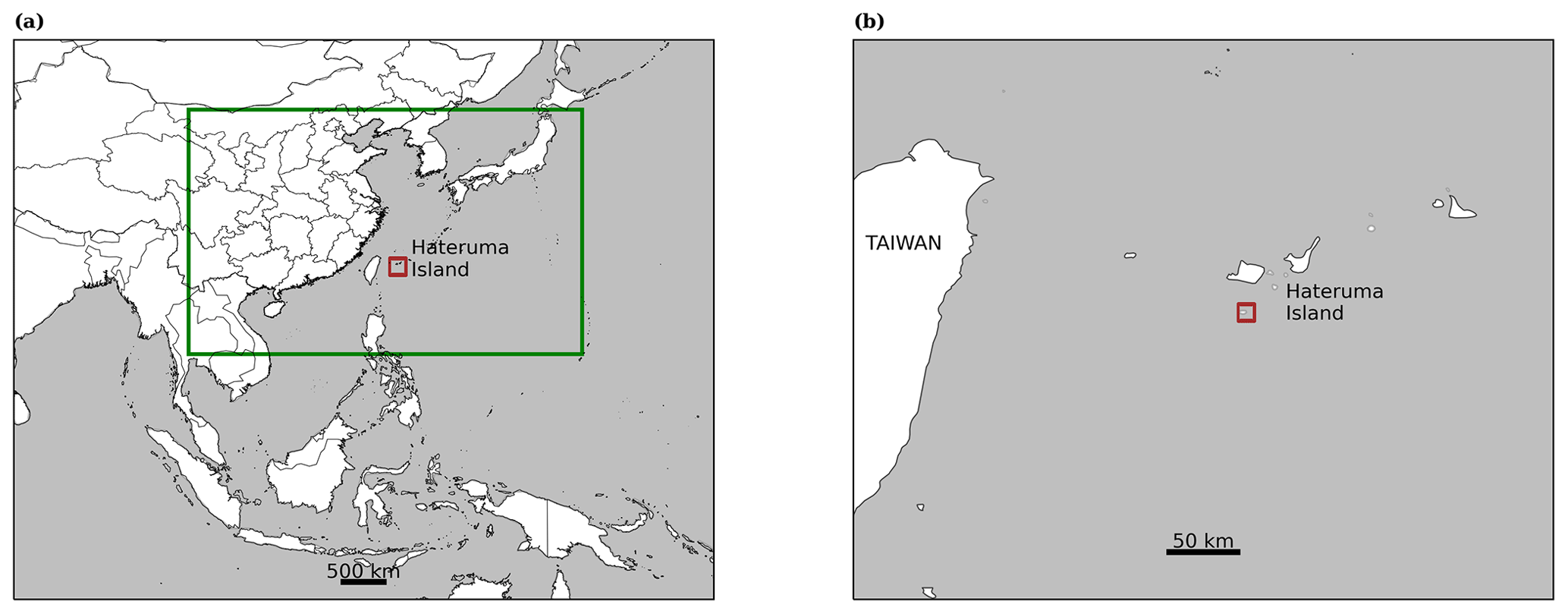
Figure 1 (a) The region of the high-resolution modelling domain spans from 14 to 42^∘ N and 100 to 145^∘ E, indicated by the green box; (b) zoomed-in image to show the location of the island of Hateruma: 24.05^∘ N, 123.80^∘ E, inside the red square.

Here we use a chemical transport model (GEOS-Chem) together with observations of the key atmospheric gases (CO, C₂H₆, C₃H₈, NO, NO₂, NO_y and O₃) measured at the observatory in Hateruma in 2018 to evaluate the model's ability to simulate the long-range transport of key species to the island of Hateruma and our understanding of emissions in the region. We start with a description of the observations made at the site (Sect. 2) and provide a meteorological context for the observations using back trajectories. We then describe the GEOS-Chem model configuration in Sect. 3 and show an evaluation of the model performance in Sect. 4. Based on this evaluation we assess the sensitivity of the model to biomass burning emissions in Sect. 5, and in Sect. 6 we explore scaling anthropogenic Asian C₂H₆ and C₃H₈ emissions to better reflect the observations at the site. We draw conclusions in Sect. 7.

2 Observations and meteorological context

In this section, we describe the observations made at the site used for this study and the meteorological context of the air arriving at the site.

2.1 Observations

The observatory is located on the eastern corner of the island, with a disused airport and the populated area (with electricity generation from diesel engines and wind power) located to the west. We expect limited local anthropogenic emissions on the island because of its small size and population. The location of the population and power generation to the west of the observations also limits potential contamination at the site from most wind directions. A number of different observations are made at the site, but we are only concerned with a subset of the observations in this study. Table 1 gives the observations used in the study and the method used to make them. Observations are available hourly for most of 2018 with some missing periods.

Shirai et al. (2010)Shirai et al. (2010)Tohjima et al. (2014)Saito et al. (2010)Saito et al. (2010)

Table 1 Physical and chemical variables measured hourly at Hateruma between 1 January to 31 December 2018 (see references for QA/QC information). Data capture indicates the number of hours when observations are available out of the 8760 h for the year.

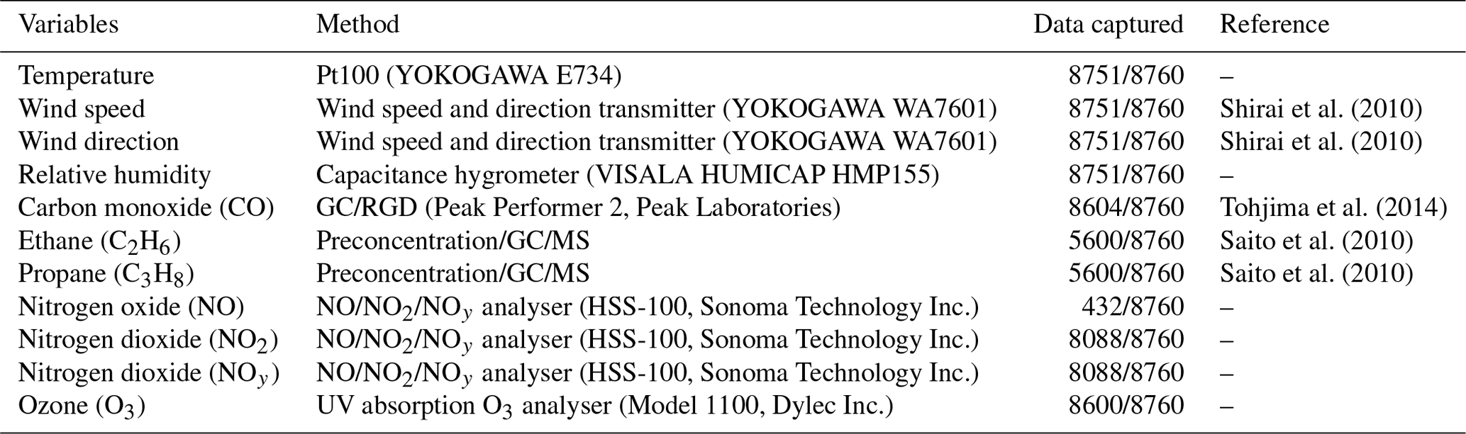
Measurements of CO, ethane and propane were made with outside air drawn from a main tower (sampling inlet: 36.5 m above ground and 46.5 m above sea level). CO was measured with a gas chromatograph–reduction gas detector (GC/RGD; Peak Performer 2, Peak Laboratories) (Tohjima et al., 2014). Ethane and propane were measured with an automated preconcentration–gas-chromatography–mass-spectrometry (GC/MS) instrument (7890B/5977B, Agilent Technologies) designed for hourly measurements of natural and anthropogenic halocarbons (Yokouchi et al., 2006; Saito et al., 2010). Ethane and propane measurements were calibrated using a gravimetrically prepared standard gas (Taiyo Nippon Sanso Co. Ltd.).

Air for $\mathrm{NO}/{\mathrm{NO}}_{\mathrm{2}}/{\mathrm{NO}}_{\mathit{\text{y}}}$ and O₃ measurements was drawn from a sub-tower (sampling inlet: 14.8 m above ground and 24.8 m above sea level). Measurements of NO, NO₂ and NO_y were made by HSS-100 (Sonoma Technology Inc. (STI)) with a blue light converter for NO₂ (NO_x converter) and a molybdenum converter for NO_y (NO_y converter) (Galbally, 2020). The conversion efficiencies of the converters were monitored daily with NO₂ gas (≈ 5 ppb) generated by a gas dilution system with gas phase titration (NO_x: 79±3 %, NO_y: 98±1 %). The detection limit of the NO measurement was about 2 ppt for 1 min acquisition. Ozone concentration was measured by UV absorption (Dylec 1100, Dylec Co., Ltd), which was calibrated with Standard Reference Photometer No. 35 (National Institute for Standard and Technology) located at NIES.

2.2 Meteorological context

Over the course of 1 year, the observatory is exposed to air masses from a wide range of locations. We calculate 10 d back trajectories for the site every hour from January to December in 2018 (52 weeks duration) using meteorological data from NCEP Global Forecast System (National Centers for Environmental Prediction, National Weather Service, NOAA, U.S. Department of Commerce, 2015) and the FLEXible PARTicle dispersion model (FLEXPART)  (Stohl et al., 2003, 2005).

Figure 2b shows the ratio of the time that these 10 d trajectories spent over the different regions shown in Fig. 2a. Over the year, most of the air is oceanic in origin from either the North or South Pacific (43 % and 34 %). However, the air masses can also spend a significant fraction of time over inland China (3.6 %), Russia (4.6 %), Korea (1.7 %), Japan (3.9 %), South-East Asia (3.1 %), the Philippines (1.2 %) and the three east China city regions (Beijing, Shanghai, Hong Kong) (3.7 %).

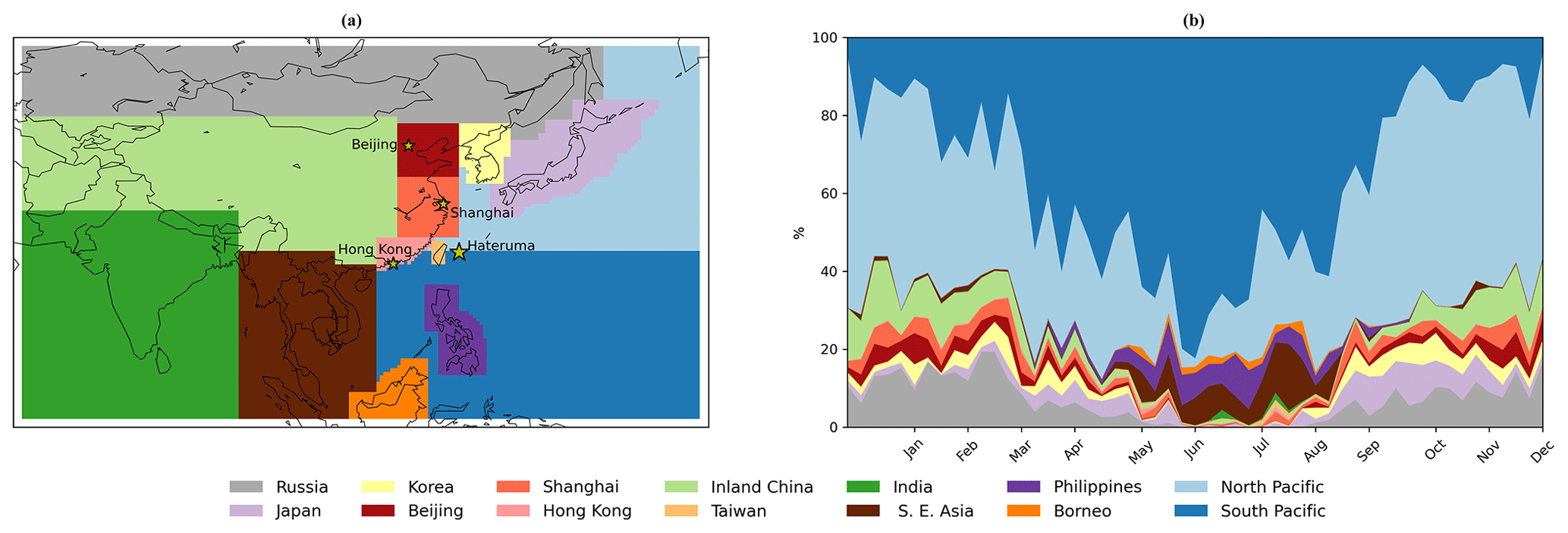
Figure 2 Trajectory analysis of air arriving at Hateruma: (a) location of the regions analysed; (b) weekly average percentage of time air masses spent over these regions.

There is, however, significant seasonal variation in air mass origin. The fraction that is oceanic (North and South Pacific) is lowest in the winter at around 60 % and is more prevalent in the summer at around 80 %. There is a shift in origin from the North Pacific region in the winter to the South Pacific region in the summer. This pattern can be attributed to the annual meteorological cycle of this region characterized by the East Asian monsoon seasons (Shirai et al., 2010; Yokouchi et al., 2006, 2011, 2017). For the remaining 20 %–40 % of the time, flow from China, Japan, Korea and Russia dominates in the winter, spring and autumn. During the summer months (April to August), the air originates from a southerly direction (Philippines, South-East Asia, Borneo).

The site is therefore mainly subject to relatively clean oceanic air with occasional exposure to air from Russia, Korea and China in the winter and the Philippines, South-East Asia and Borneo in the summer.

3 Chemical transport model configuration

We use a chemical transport model, GEOS-Chem version 12.7.1 (https://doi.org/10.5281/zenodo.3676008, The International GEOS-Chem Community, 2020) to help analyse the measurements made at Hateruma. The model was first described by Bey et al. (2001) but has had substantial improvements since then (https://geoschem.github.io/, last access: 11 August 2023). We use a regional simulation with a spatial resolution of 0.5^∘ × 0.625^∘ over the domain shown in Fig. 1a. The model includes a detailed HO_x–NO_x–VOC-ozone–halogen–aerosol tropospheric chemistry as described by Sherwen et al. (2016) and is driven by offline meteorology from the NASA Global Modelling and Assimilation Office (http://gmao.gsfc.nasa.gov, last access: 5 September 2021) forward-processing product (GEOS-FP).

To generate restart files and boundary conditions, the model was run in a global configuration at a 4^∘ × 5^∘ horizontal resolution for 2 years (1 January 2017–1 January 2019) with the first year regarded as spin-up. We then run the model in its regional configuration using the boundary conditions derived from the global simulation and output the result every hour. Figures A1–A4 in the Appendix show a comparison between the model simulations run at the native meteorological resolution of 0.25^∘ × 0.3125^∘ and the simulation run at 0.5^∘ × 0.625^∘. The differences between the two models are minimal, so we adopt the coarser 0.5^∘ × 0.625^∘ resolution version as it is substantially faster to run with only a small degradation in performance.

We run the model in a slightly different emission configuration than its default. We use the Community Emissions Data System (CEDS) emissions with applied monthly and diurnal variability as described in Hoesly et al. (2018) for all anthropogenic emissions other than for those from aircraft where we use the Aviation Emissions Inventory Code (AEIC) (Stettler et al., 2011). This contrasts with the model default configuration which uses Tzompa-Sosa et al. (2017) and Xiao et al. (2008) for anthropogenic ethane and propane emissions but does makes our simulation consistent with recent Coupled Model Intercomparison Project (CMIP) model evaluations (Griffiths et al., 2021). The CEDS emissions were available at 0.1^∘ resolution and the Harmonized Emissions Component (HEMCO) module (Keller et al., 2014; Lin et al., 2021)) interpolates all emissions to the grid resolution (0.5^∘ × 0.625^∘) of the model.

We also include geological emissions of ethane and propane that may represent a normally missing source (Etiope et al., 2019; Dalsøren et al., 2018). We assume a global total of 3.0 Tg yr⁻¹ of ethane and 1.7 Tg yr⁻¹ of propane (Dalsøren et al., 2018). We spatially distribute these emissions using a geological methane emission dataset (Etiope et al., 2018). This source represents only 10 %–20 % of the global emissions of both ethane and propane, and we do not believe that these geological emissions are of specific importance for this region.

Other emissions include offline soil NO_x (Weng et al., 2020) and online lightning NO_x emissions (Murray et al., 2012). The PARANOX ship plume model by Holmes et al. (2014), which calculates the ageing of emissions in ship exhaust plumes for NO_x, HNO₃ and O₃ was applied to the CEDS shipping emissions  (Hoesly et al., 2018). Biomass burning emissions use the Global Fire Emissions Database GFED 4.1 (Andreae and Merlet, 2001; Akagi et al., 2011; Giglio et al., 2013; Randerson et al., 2012; van der Werf et al., 2017). Biogenic emissions follow the estimation from the Model of Emissions of Gases and Aerosols from Nature (MEGAN) 2.1 (Guenther et al., 2012). The natural emissions of acetaldehyde follow the calculation from Millet et al. (2010). Natural sources of NH₃ are adapted from the Global Emission InitiAtive (GEIA) as described by Bouwman et al. (1997), with the inclusion of the Arctic seabird emissions (Riddick et al., 2012).

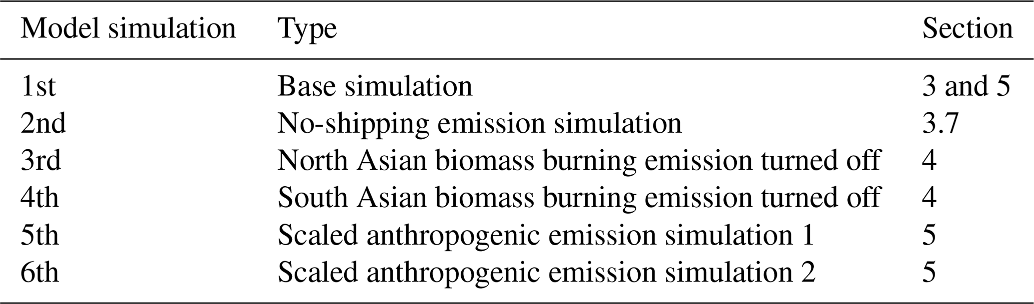
Table 2 gives the list of simulations performed and the sections in which these simulations are discussed.

Table 2 Summary of GEOS-Chem model simulations and reference sections.

4 Model results and performance

In order to assess the veracity of the GEOS-Chem model simulation we compare its performance: first against the meteorological observations made at the site and then against measurements of atmospheric chemical constituents. Since the model and observation data are available hourly and observation data capture is high in most cases, instances of missing data were dropped for both the observation and the model before comparison. The observation data were adjusted from Japan standard time (JST) to model default time (UTC). We compare hourly values from the observations and from the model for the physical and chemical variables except for NO, NO₂ and NO_y, where we compare local daylight averages due to high variability.

We use a number of standard metrics for describing the measurements and model (mean, median, standard deviation, 25th and 75th percentiles). When assessing the model performance we assess this in terms of the root mean square error (RMSE), mean bias and Pearson's correlation coefficient (r). We also calculate the slope of the best-fit lines using orthogonal distance regression (ODR).

In the case of wind direction, which is circular and not linear, the methodology for the estimation of RMSE and bias follows Ferreira et al. (2008) and Carvalho et al. (2012).

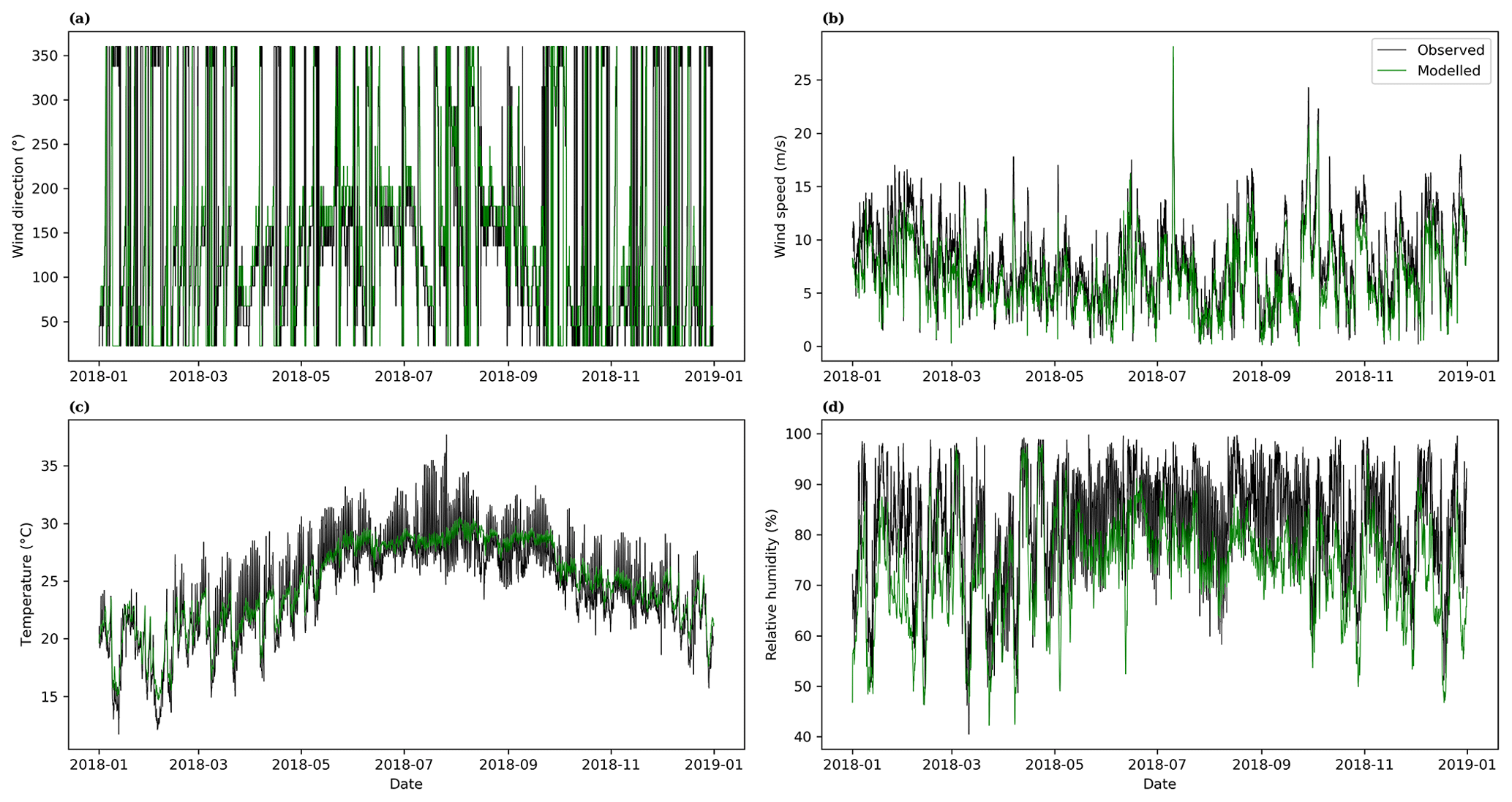
Figure 3 Observed and modelled (a) wind direction, (b) wind speed , (c) temperature and (d) relative humidity at Hateruma.

4.1 Meteorological variables

Figure B1 in Appendix B shows the wind rose representing observed and modelled wind speed and direction at the site. As the populated part of the island lies to the west of the site, this highlights that the local contamination is likely small. Figure 3 shows a comparison between the hourly observed and modelled time series for wind speed, wind direction, temperature and relative humidity at the observatory.

The wind direction (10 m above surface) is plotted in Fig. 3a as the incidence angle of the wind (north: 0 and 360^∘). The observations are given with a resolution of 22.5^∘ clockwise, which gives them a blocky appearance. Overall, the model captured the observed wind direction well throughout the year with few discrepancies. The modelled wind direction has a low RMSE (6.5^∘) and a slightly positive bias (6.5^∘). This could be attributed to a small error in meteorological fields used in our simulations or to potentially a small error in the measurements. The seasonal variability in wind direction is well represented in Fig. 3b, with the summer time characterized by winds coming from the south and the winter having winds from a more northerly direction.

The modelled wind speed has a correlation coefficient (r) of 0.90 and a RMSE of 2.17 m s⁻¹ (Fig. 3b). The wind speeds are lower in the model (mean of 6.43 ± 3.12 (1σ) m s⁻¹) than in the observations (mean of 7.83 ± 3.79 (1σ) m s⁻¹). This may reflect local reductions in wind speed over the island due to increased surface drag not being represented in the model due to its grid resolution.

Surface temperatures (2 m above surface) show a high degree of correlation (r=0.92) and a RMSE of 1.75 ^∘C, with the mean observed surface temperature (24.53 ± 4.27 (1σ) ^∘C) close to that simulated (24.76 ± 3.67 (1σ) ^∘C). There is, however, significant hourly variation not captured by the model (Fig. 3c). This again could be due to resolution impacts at different scales since the island is smaller than the model grid box at Hateruma. Local heating and cooling at the observatory and the island will not be represented in the model fields.

The modelled surface relative humidity (RH at 2 m above the surface in Fig. 3d) is less well captured (r=0.77; RMSE = 11.26 %), with the modelled mean (73.09 ± 9.89 (1σ) %) lower than the observed mean (82.00 ± 10.32 (1σ) %). This difference could again be attributed to the sub-grid issues where the meteorology used in the model is on a fairly coarse scale compared to the observations.

In general, the model performance compared to the meteorological observations is relatively good, reflecting the observational data assimilated into the GEOS-FP meteorological fields. We can now assess the model performance in simulating the mixing ratio of the trace gases observed at the site.

4.2 Carbon monoxide

Figure 4a (left) shows the time series of CO measured and modelled at the site, with Fig. 4a (right) showing the correlation between the hourly modelled and measured values. Mixing ratios are highest in the winter months reflecting transport from north Asia (China, Korea, Japan) and the North Pacific (Fig. 2) and lower oxidation by OH in the winter months (Schlesinger and Bernhardt, 2020). The mixing ratios are lower in the summer reflecting transport from southern regions (they are further away and typically have lower emissions) and increased oxidation due to enhanced OH concentrations in the summer (Schlesinger and Bernhardt, 2020). Koike et al. (2006) measured CO in northern Japan and reported a similar seasonality in CO mixing ratios over the year.

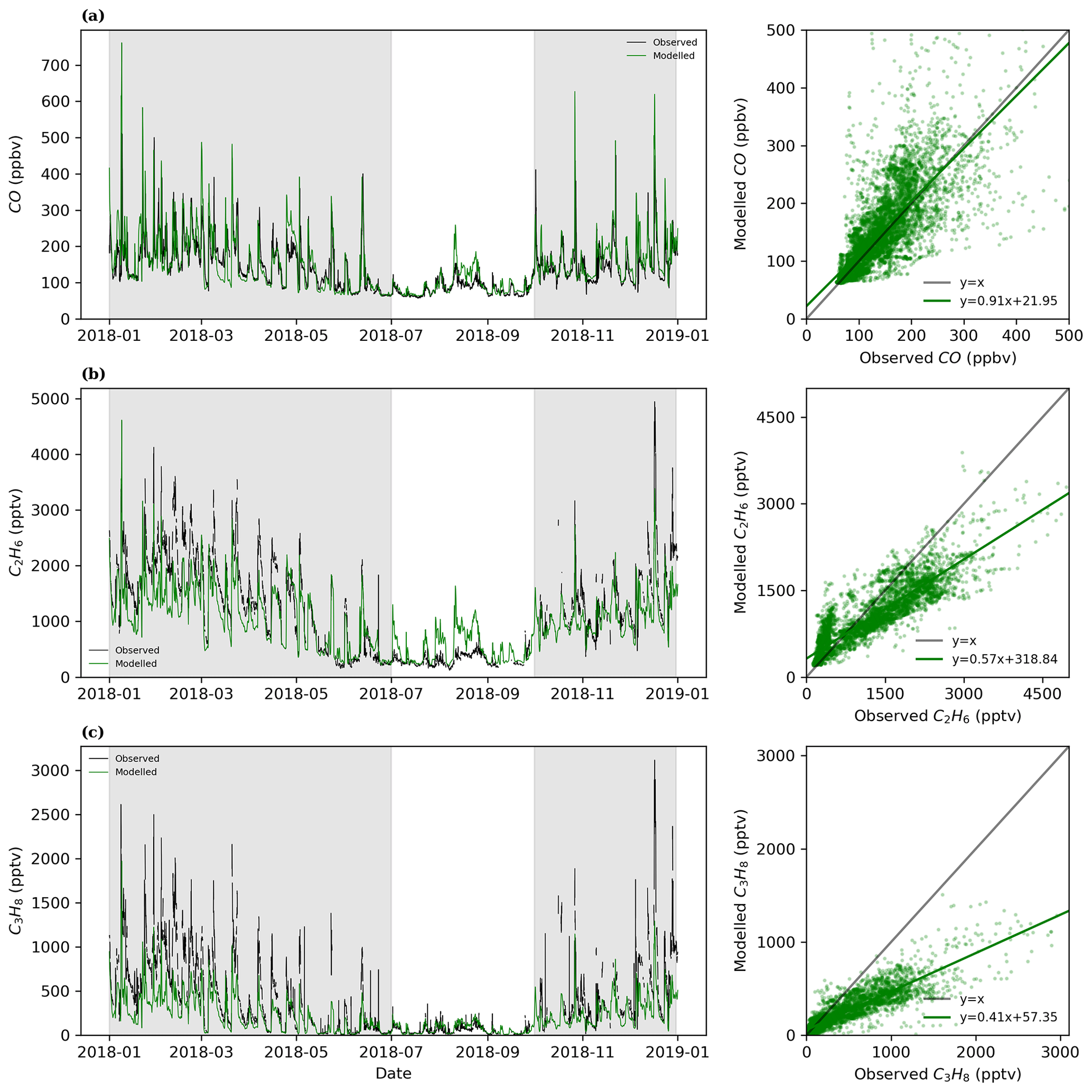
Figure 4 Modelled and measured hourly (a) CO, (b) C₂H₆ and (c) C₃H₈ mixing ratios calculated for the Hateruma site.

Over the year, the model simulates the CO mixing ratio well with a mean value of 146 ± 77 (1σ) ppbv compared to mean observations of 136 ± 62 (1σ) ppbv. The median CO mixing ratios calculated and measured are 127 and 122 ppbv, respectively. The 25th and 75th percentile modelled is 89 and 180 ppbv compared to 89 and 169 ppbv observed. There is a good degree of correlation (r=0.74) between the model and measurements with a RMSE of 53 ppbv and the line of best fit having a slope of 0.91.

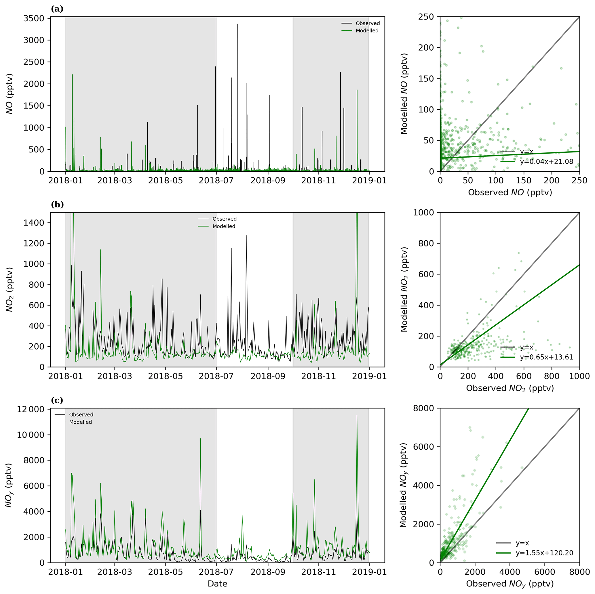
Figure 5 Modelled and measured mean daytime (a) NO, (b) NO₂ and (c) NO_y mixing ratios calculated for Hateruma.

4.3 Ethane

Similar to CO, the highest observed ethane (C₂H₆) mixing ratios occur in the winter, while the mixing ratios in the summer are substantially lower (Fig. 4b – left). The model results underestimate the mean mixing ratio (972 ± 541 (1σ) pptv) compared to the observations (1188 ± 842 (1σ) pptv)) with a RMSE of 481 pptv. Also, a median mixing ratio is calculated to be 942 pptv, with a 25th to 75th percentile spread of 552–1386 ppbv, while the median from observation is 1134 pptv with a spread of 368–1825 pptv. This underestimate in modelled ethane results is most noticeable in the winter months. However, in the summer the model outputs can give overestimates. This leads to two populations in the model–measurement scatter plot (Fig. 4b – right) with a strongly correlated but overestimated population at observed mixing ratios below 500 pptv (in the summer) and another population with underestimated mixing ratios above this (in winter). The correlation coefficient between model outputs and measurements is relatively high at 0.88, but the linear fit between model results and measurements is dominated by the wintertime underestimate to give a slope of 0.57.

4.4 Propane

Figure 4c (left) shows the comparison between the measured and modelled time series for propane (C₃H₈). A similar pattern to C₂H₆ is seen with high wintertime mixing ratios and much lower values in the summer. Unlike C₂H₆ though, a summer time overestimate is not evident. The model captures much of the variability in the C₃H₈ mixing ratios with a correlation coefficient of 0.89 (Fig. 4c – right). The mean mixing ratio of C₃H₈ is 391 ± 432 (1σ) pptv for the measurements and 210 ± 198 (1σ) pptv for the model. The median C₃H₈ mixing ratio calculated and measured is 156 pptv (25th and 75th percentiles of 69 and 335 pptv) and 221 pptv (25th and 75th percentiles of 62 and 611 pptv), respectively. The RMSE is 320 pptv, and the slope of the linear fit between calculated results and measurements is 0.41. Thus, similar to the situation with C₂H₆, the model substantially underestimates C₃H₈ mixing ratios.

4.5  NO_x

Here, we evaluate the model's performance in simulating NO and NO₂ (collectively known as NO_x). The short lifetime of NO and NO₂ (on the order of minutes to hours during the day) makes evaluation against model data difficult due to large and rapid variations. During the day NO mixing ratios are high due to the photolysis of NO₂. During the night, away from recent emissions, its mixing ratios are effectively zero. For this evaluation, we compare mean day values (06:00 to 18:00 local time) between the model results and observations. Figure 5a shows the comparison between the measured and modelled daytime mean for the NO mixing ratio. The mean observed value (7 ± 28 (1σ) pptv) is substantially lower than the modelled value (21 ± 41 (1σ) pptv). The model also shows very little skill in the day-to-day variability with an r of 0.03 and a slope of 0.5 for the linear fit.

Figure 6 Modelled and measured hourly O₃ mixing ratios calculated for the Hateruma site.

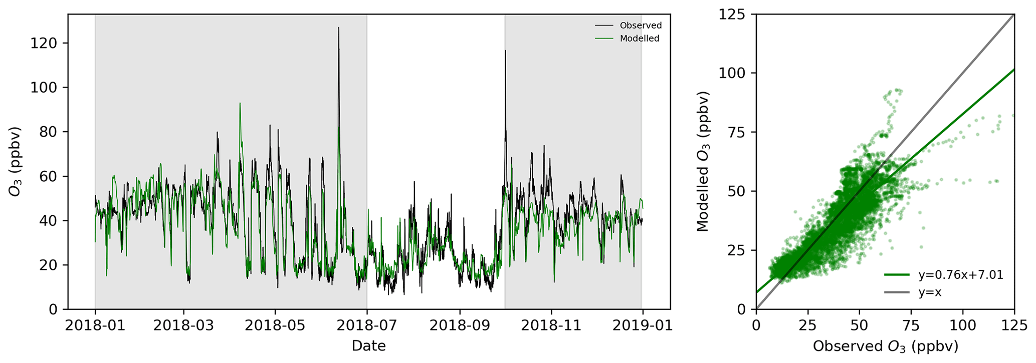
Figure 5b (left) compares the time series of daily average NO₂ between the measured and modelled, with Fig. 5b (right) showing the relationship as a scatter plot and best-fit line. The model simulates NO₂ better than NO. The mean NO₂ mixing ratio measured is 260 ± 185 (1σ) pptv, while the modelled NO₂ mean mixing ratio is 182 ± 323 (1σ) pptv. The median NO₂ mixing ratio observed is 198 pptv with a 25th and 75th percentile range of 127 and 335 pptv, whereas the calculated ratio is 121 pptv, with a 25th to 75th percentile range of 97 and 152 pptv. The correlation coefficient between observation and measurement is, however, low (0.36) with a RMSE of 322 pptv, and the slope of the linear fit is 0.65.

Generally, the model performance for the NO_x species is poorer than for other species. This likely reflects a number of problems. It is difficult to make observations at these low concentrations (Reed et al., 2016), and for many days the NO observations are below the detection limit. It also likely reflects the short lifetime of NO_x making it susceptible to local chemical and emissions processes which the model cannot resolve. Summer NO and NO₂ observed at Hateruma is higher than model estimates, which is similar to the observations by Han et al. (2019) over Mongolia where thermally decomposed peroxyacetyl nitrate (PAN) during the warmer season contributes to higher NO₂ levels in remote regions. However, in general the modelled NO_x at Hateruma (dominated by NO₂) underestimates the observed values.

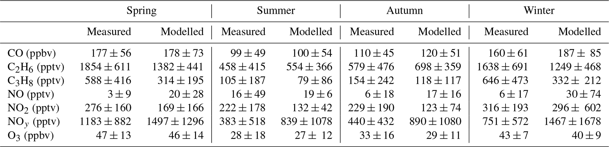
Table 3 Mean and standard deviations in mixing ratios of measured and modelled species over different seasons between 1 January 2018–31 December 2018.

4.6 NO_y

Figure 5c (left) shows the daily average measured and modelled time series for gas phase reactive nitrogen species (NO_y). We define here NO_y for the model as NO + NO₂ + 2×N₂O₅ + HNO₂ + HNO₃ + PAN (which will tend to marginally underestimate the true modelled NO_y as it misses halogen nitrates and some other minor constituents such as NO₃ and some organic nitrates). We assumed that none of the particulate nitrate is measured. Figure 5c (right) shows the scatter plot with the line of best fit between measurements and calculations. The mean observed NO_y mixing ratio is 683 ± 698 (1σ) pptv, while the mean modelled NO_y mixing ratio is 1173 ± 1340 (1σ) pptv. The correlation coefficient between observation and model calculations is 0.79 with a RMSE of 1035 pptv. The slope of the best-fit line is 1.55. Thus, the model appears to overestimate NO_y mixing ratios by roughly 50 % despite not including some of the NO_y species and the potential for some particulate NO_y being sampled by the observations. The model performance is better than for NO_x. However, whereas the NO_x appears to be underestimated in the model, the NO_y is overestimated. HNO₃ and PAN are dominant in the model-estimated NO_y levels at Hateruma. Thus, the NO_y overestimate and the NO_x underestimate could be related to NO₂ formation and loss pathways (Han et al., 2019).

A simulation without shipping emissions within the high-resolution domain reduces NO_y mixing ratios by 25 %. Thus, even switching off these emissions entirely does not compensate fully for the model overestimate and makes the model underestimation of NO_x worse. It is therefore unclear why the model overestimates the NO_y mixing ratios. This could indicate excessive emissions in the region, too long a modelled NO_y lifetime or some difficulty in the model chemistry. Further work will be necessary to understand NO_x and NO_y in the region.

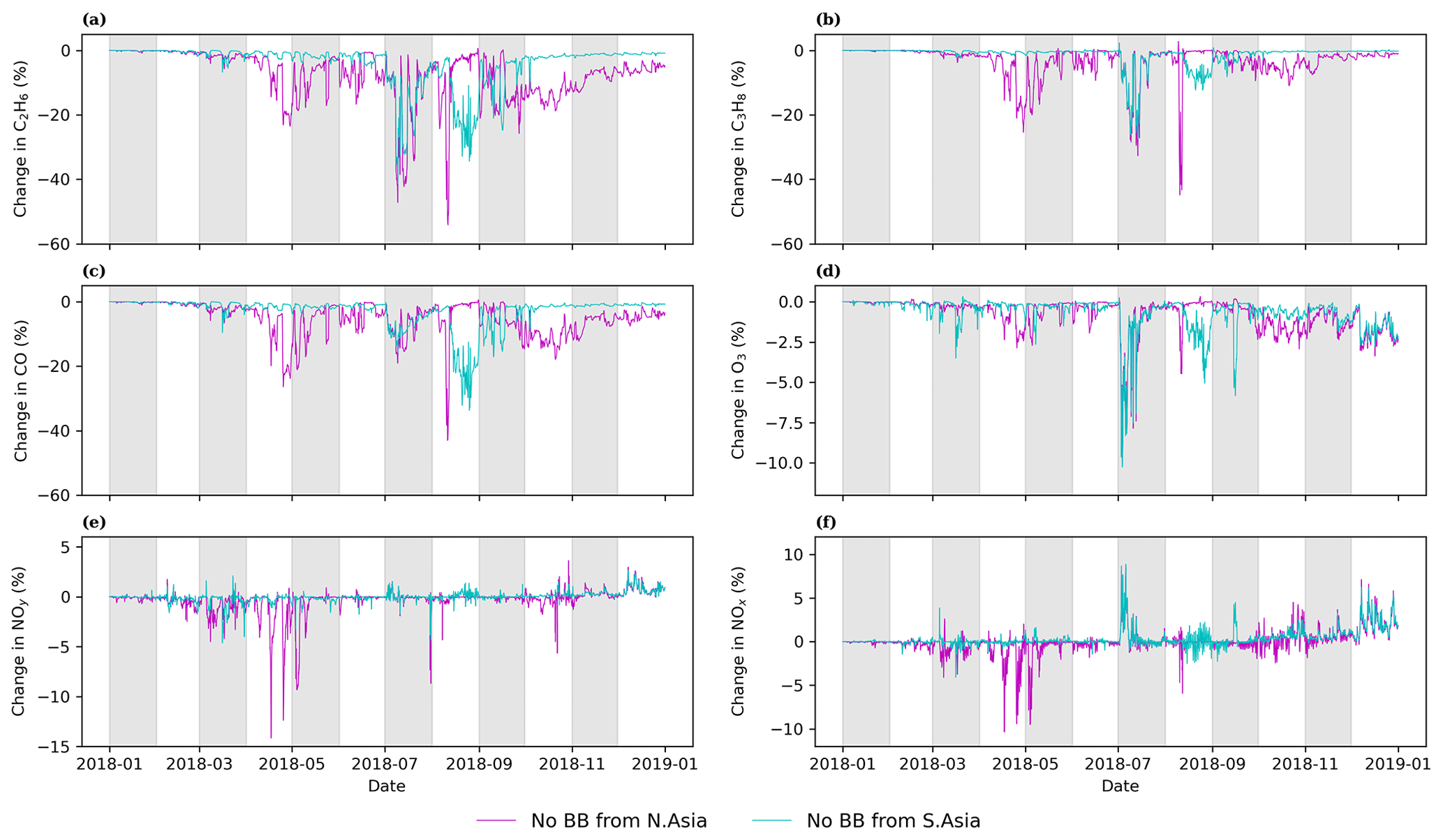
Figure 7 Percentage change in (a) C₂H₆, (b) C₃H₈, (c) CO, (d) O₃, (e) NO_y and (f) NO_x mixing ratios between standard and simulations without north Asian or south Asian biomass burning.

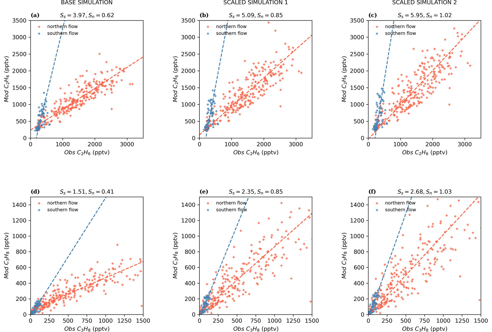
Figure 8 C₂H₆ and C₃H₈ modelled plotted against measurements in the base simulation (a and d) and scaled anthropogenic emission simulations with initial correction factor (b and e) and optimized correction factor (c and f). Data are split into a southern-flow period (July–September) in blue and a northern-flow period (October–June) in red. S_s and S_n give the slope of the line of best fit for the time series in southern- and northern-flow periods, respectively.

4.7 Ozone

Figure 6 (left) shows the measured and modelled time series for O₃. In general, the model performs well (RMSE of 8 ppbv; mean measured O₃ of 38 ± 16 (1σ) ppbv; mean model O₃ of 36 ± 14 (1σ) ppbv) and simulates much of the variability with a correlation coefficient (r) of 0.87. However, the line of best fit between observations and model results is low, with a slope of 0.76 (Fig. 6 – right). The median O₃ mixing ratio calculated is 35 ppbv (25th and 75th percentiles of 22 and 46 ppbv), whereas the corresponding measurement is 40 ppbv (25th and 75th percentiles of 24 and 49 ppbv).

During the summer, there are periods of low O₃, reaching 6.5 ppbv. The model fails to capture these low mixing ratios and simulated a minimum of 10 ppbv. Conversely, in the winter months, the model reproduces much of the variability but has a tendency to underestimate the observed mixing ratios. Overall, this leads to overestimates for low mixing ratios and underestimates for high mixing ratios. Thus, there is a reduced slope of the linear fit in the scatter plot (Fig. 6).

4.8 Summary

In general the model has some skill at picking out the variations in meteorological history of the air masses arriving at the site, reflected in the generally high correlation coefficients between the model and the measurements. This mainly reflects the quality of the data assimilation used in the NASA-generated meteorological fields. The success in simulating the absolute mixing ratios is more varied. Table 3 summarizes the mean calculated and measured mixing ratios for spring (February–April), summer (May–July), autumn (August–October) and winter (November–January).

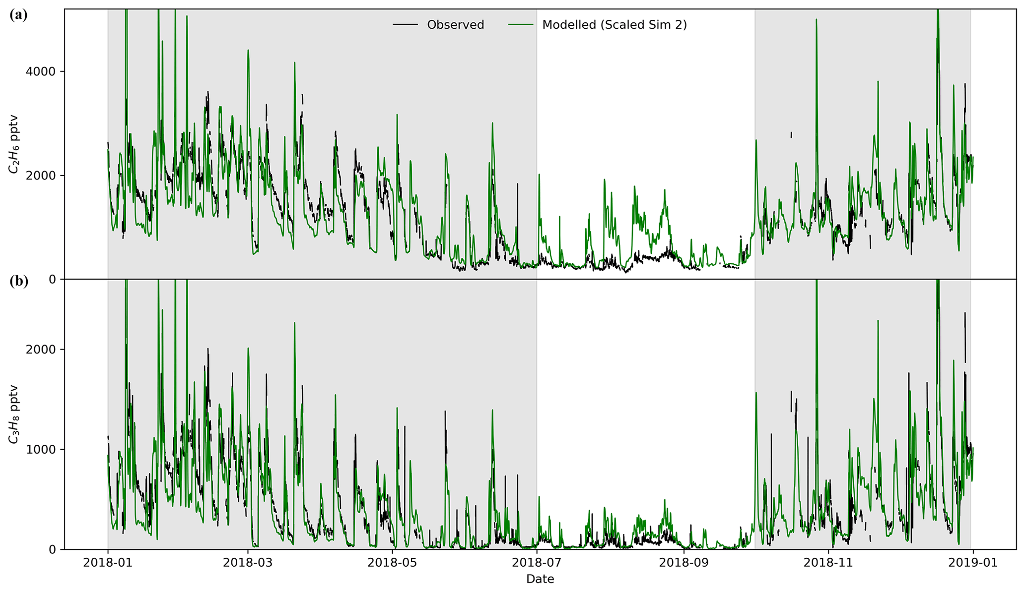
Figure 9 Time series of hourly C₂H₆ (a) and C₃H₈ (b) observed and modelled mixing ratios (scaled anthropogenic emission simulation 2).

There is a clear seasonality in the observations at Hateruma, and this is similar to other oceanic sites in East Asia. Such a seasonality is reported at Cape Ochi-ishi (43^∘10′ N, 145^∘30′ E) and the Oki Islands (36^∘17′ N, 133^∘11′ E), where Asian outflows amplifies the winter concentrations of hydrocarbons (Tohjima et al., 2002; Sharma et al., 2000). While NO_x has a very short atmospheric lifetime and its formation and loss are related to NO_y species such as HNO₃ and PAN, it is reported to have different seasonality in polluted and remote regions (Han et al., 2019).

As shown in Table 3, carbon monoxide mixing ratios are relatively well simulated in all seasons with a small bias toward high values in the autumn and winter. Ethane is underestimated in the spring and winter but overestimated in the summer and autumn. Propane mixing ratios are underestimated in all seasons. NO_y observations are overestimated by the model, whereas NO and NO₂ mixing ratios are underestimated.

Although the largest divergences in the model results compared to observations are found for NO_x and NO_y species, there is uncertainty about the accuracy of these measurements at such low mixing ratios. Thus, we focus on the hydrocarbons in which we have more confidence. The model underestimates C₂H₆ and C₃H₈ mixing ratios especially in the spring and winter. We therefore conduct a number of model experiments to investigate these observations. We first run simulations to assess the role of biomass burning in controlling the mixing ratios of these species at the site, we then assess how much the Asian anthropogenic source of these compounds would have to increase by in order to give agreement between the model and the measurements in the winter months.

5 Biomass burning sources

In order to understand the impact of biomass burning on the composition of the air arriving at the site, we conduct an additional simulation, switching off the biomass burning emissions from north Asia and South Asia separately as shown in Fig. B2. Two global simulations were run switching off the northern or southern Asian biomass burning to generate new boundary conditions, and then these were used for the two regional simulations which again switched off the biomass burning in either the north or south of Asia.

Figure 7a–f show the time series of the percentage change in modelled mixing ratios of C₂H₆, C₃H₈, CO, O₃, NO_x and NO_y at the site when biomass burning emissions in either the northern or southern domain are switched off. Given the short lifetime of NO_y and NO_x, the site is less sensitive to biomass burning NO_x than CO, C₂H₆ and C₃H₈, and Fig. 7d and f show the correlation between O₃ and NO_x when less ozone is formed due to switching off emissions, more NO_x is accumulated.

During the winter months the contributions from north and South Asia are relatively small; however, in the summer, both sources can contribute significantly (20 %–35 %) to the modelled C₂H₆, C₃H₈ and CO. The contributions are smaller for O₃ reaching a maximum at 10 % during events in the summer. There is a sharp dip around 10 August where CO, C₂H₆ and C₃H₈ levels drop by around 40 %–50 % due to switching off north Asian biomass burning emissions. After this sharp dip, the next decline from 16 August was more sustained and due to South Asian biomass burning emission. These sharp dips correspond to the passing of typhoons in the area, which can rapidly draw air from different direction for short period of time. Figure B3 shows the back-trajectory analysis for this period when the wind direction rapidly changed. There is also a tendency for increased Asian fire activity in the summer which explains why the strong and rapidly changing wind would bring in more emissions.

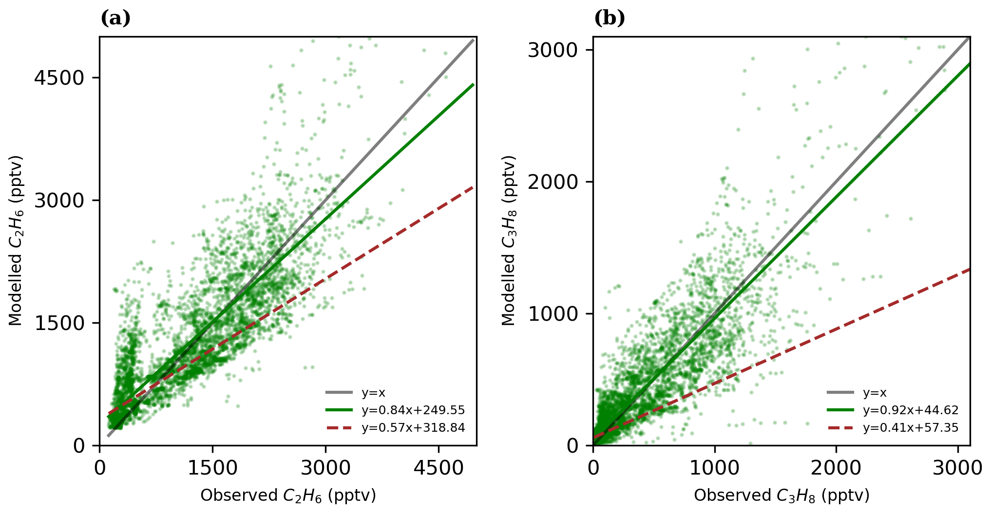
Figure 10 Scatter plot showing hourly (a) C₂H₆ and (b) C₃H₈ mixing ratios between observation mixing ratios and model calculations with scaling (scaled anthropogenic emission simulation 2). Red dashed line shows best-fit line before scaling.

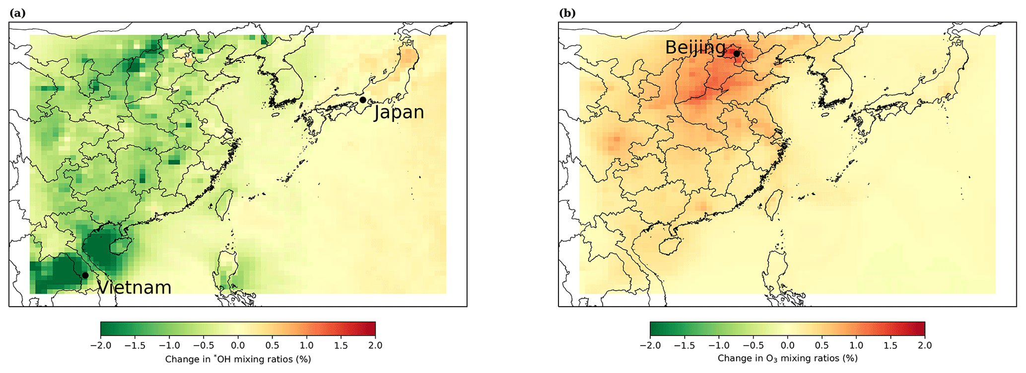
Figure 11 Percentage changes in average July mixing ratios of (a) OH and (b) O₃ after increasing Asian ethane and propane anthropogenic emissions.

The periods of model overestimate in summer ethane, notably in August (Fig. 4b), correspond to periods with a high fraction of modelled ethane biomass burning (∼ 30 %). However, the model overestimate (see Fig. 4b) is much large than this (∼ 100 %). Thus, even if the biomass burning is switched off all together, the model overestimate during the summer would still remain. This suggests that the model overestimate of C₂H₆ in the summer is not primarily related to the modelled representation of biomass burning but likely results in uncertainties in the anthropogenic emissions of ethane south of Hateruma.

During the wintertime the model underestimates the observed ethane and propane. This is a period when the contribution from biomass burning is relatively low (<10 %). Thus the potential for the underestimate in wintertime ethane and propane to be related to errors in the biomass burning appears to be small. Instead, we now evaluate how much the Asian anthropogenic source of ethane and propane would have to be increased by in order to fit the observed mixing ratios.

6 Anthropogenic emissions

The period between October to June (Figs. 4–6) is characterized by elevated levels of pollution at the site due to flow from Russia, China, Korea and Japan (Fig. 2). It is also a period when the model substantially underestimates the mixing ratios of ethane and propane. In this section we explore what scaling factor would have to be applied to the Asian anthropogenic emissions of ethane and propane within the high-resolution domain to better fit those observations.

Figure 8a and d show modelled ethane and propane plotted against observations in our base model. We separate the plot into two periods here as southern flow (blue, July–September) and northern flow (red, October–June). It is obvious from the comparison that during the northern-flow period, the model-measured slope is lower than expected (0.62 for ethane and 0.41 propane), whereas in the southern-flow period it is substantially overestimated for ethane (3.97) and to a smaller extent also for propane (1.51).

Given the site's largest exposure to relatively recent north Asian emissions in the northern-flow period, we focus on this. We multiply the Asian anthropogenic emission of ethane and propane within the high-resolution domain by a first rough estimate of a correction factor “A” (1.75 for ethane and 2.58 for propane, which are roughly the reciprocal of the model– measurement slopes show in Fig. 8, i.e. 1$/$0.62 and 1$/$0.41) aimed at making the slope of the linear fit in the northern-flow period become 1. This would represent a correction factor if all of the ethane and propane observed at the site were from within the high-resolution simulation domain and the oxidation lifetimes were correct.

The annual simulation was re-run with the anthropogenic emissions of ethane and propane increased by the A factor within the “Asian” high-resolution domain (Fig. 8b and e). Assuming a linear response, these two simulations allow the mixing ratios of ethane and propane in the base simulation to be represented as $\left[X\right]=[X{]}_{\mathrm{Asian}}+[X{]}_{\mathrm{Rest}\mathrm{of}\mathrm{the}\mathrm{world}}$ and the mixing ratios in the simulation with increased emissions to be represented as $\left[X\right]=\mathrm{1.75}\times [X{]}_{\mathrm{Asian}}+[X{]}_{\mathrm{Rest}\mathrm{of}\mathrm{the}\mathrm{world}}$ for ethane and $\left[X\right]=\mathrm{2.58}\times [X{]}_{\mathrm{Asian}}+[X{]}_{\mathrm{Rest}\mathrm{of}\mathrm{the}\mathrm{world}}$ for propane. The base mixing ratios at each time point can then be decomposed to give an Asian component (although this is only the component within the higher-resolution domain) and a “Rest of the world” component. A scaling can then be applied, which optimizes the fit between the measurement and the model by finding an optimized multiplier for the Asian emission: A_optimized.

The value of A_optimized is found to be 2.22 and 3.17 for ethane and propane, respectively, if the best-fit line is optimized (Fig. 8). This is consistent with the value found by optimizing the ratio of mean mixing ratios in the period when the wind flow is northerly (calculated as 2.24 and 3.14, for ethane and propane, respectively). Re-running the model with these increases in the ethane and propane emissions within the domain gives a scatter plot of ethane and propane measurements versus model values in Fig. 8c and f, a time series shown in Fig. 9, and a correlation between the whole dataset in Fig. 10. The correlation coefficient (r) is slightly reduced after the scaling (0.88 to 0.84 and 0.89 to 0.86 for C₂H₆ and C₃H₈, respectively).

For the northern-flow period (October to June), when the air is predominantly off north Asia, the modelled ethane now has a mean of 1443 ± 737 (1σ) pptv compared to an observed mean of 1449 ± 725 (1σ) pptv. The propane simulation has a mean of 493 ± 418 (1σ) pptv compared to an observed mean of 494 ± 407 (1σ) pptv. During the southern-flow period (July–September), the model now significantly overestimates the ethane (mean simulated = 587 ± 352 (1σ) pptv; mean observed = 308 ± 99 (1σ) pptv) and propane (mean simulated = 105 ± 88 (1σ) pptv; mean observed = 60 ± 37 (1σ) pptv).

The improvement in model performance during the northern flow and the degradation in performance during the southern flow point towards a non-uniformity in the correction factor. This could indicate a difference in the seasonality of the emissions compared to those used in Hoesly et al. (2018) with a significant reduction in the summer time emissions compared to the winter, or it could indicate a different reason for the increase in north Asia compared to south Asia, which is primarily sampled in the summer.

The comparison of ethane and propane observations with model results shows that a large increase in the prescribed emissions of these tracers is necessary, in agreement with previous studies. Dalsøren et al. (2018) found it necessary to increase CEDS anthropogenic ethane emissions by a factor of roughly 2 and CEDS propane emission by a factor of nearly 3 to get agreement between their model and observations. These are very similar to the ratios found here. Tzompa-Sosa et al. (2017) found it necessary to substantially increase anthropogenic ethane sources to fit observations. Mo et al. (2020) measured vertical profiles of VOCs (including C₂H₆ and C₃H₈) and reported that emission fluxes were up to 3 times larger than in the Multi-resolution Emission Inventory for China (MEIC) inventory estimates. It seems likely that current estimates of north Asian emissions of ethane and propane are currently underestimated.

Figure 11a and b show the impact of the increase (with the optimized factors) in Asian ethane and propane anthropogenic emissions on the mixing ratios of average hydroxyl radical and ozone in the region in July, respectively. This is the period of the highest ozone mixing ratios over China. The effect on the OH mixing ratios in July was small and patchy with up to a 2 % reduction in some places. On the other hand, O₃ mixing ratios increased slightly, reaching a maximum over Beijing, where that amounts to a 2 % (around 1 ppbv) increase.

7 Conclusions

Measurements were made of a number of compounds in the air over the island of Hateruma (CO, C₂H₆, C₃H₈, NO, NO₂, NO_y and O₃). We show that the site is mainly subject to clean Pacific air throughout the year. If the site is subject to polluted air masses, these are more likely to have originated from north Asia (Russia, China, Japan, Korea, etc.) in the winter months and from south Asia (Philippines, Borneo and other regions in South-East Asia including Vietnam, Indonesia, peninsular Malaysia and Thailand) in the summer months. This gives the site a significant seasonal cycle in the mixing ratios of pollutants considered in this study except NO_x.

We have compared these observations to the output of the GEOS-Chem model, run in a regional configuration. We find that CO and O₃ are well simulated; the model overestimates NO_y observations but tends to underestimates NO, NO₂, ethane and propane.

The underestimates in ethane and propane during the wintry months are unlikely to be reconciled by increases in biomass burning emissions but could be reconciled by substantial (factors of 2–3) increases in the Asian anthropogenic source of these compounds (consistent with previous studies). These large increases in emissions have negligible influence on the hydroxyl radical mixing ratios and very little impact on the ozone in the region's cities such as Beijing, where there is up to 1 ppbv change in ozone mixing ratios in July.

We do not believe the overestimates of NO_y can be attributed to problems with the simulation of shipping NO_x, as even switching off the shipping NO_x emissions does not remove the overestimate. Also, biomass burning emissions can only contribute up to 10 % of NO_x levels estimated at the site; therefore, the overestimates likely lies in the emissions of NO_x from industrial regions close by, in issues with the chemistry or in the observations.

The site's location is unusual and is subject to air masses from a large number of sites and so can be used to understand emissions of compounds from a number of location. Future plans to enhance the measurement capability at the site with a gas-chromatography–mass-spectrometry system (GC-MS) should allow an evaluation of a large number of different organic compounds, further enhancing the capacity to understand sources of pollution in the region.

Appendix A: Comparison of simulation resolutions

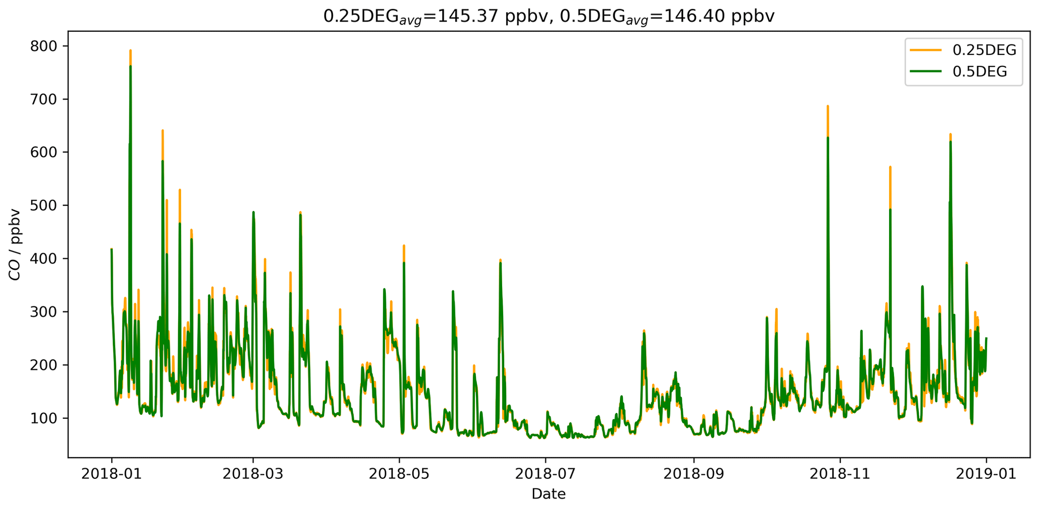
Figure A1 Modelled time series comparing CO simulation at 0.25^∘ × 0.3125^∘ and 0.5^∘ × 0.625^∘ resolution at the site.

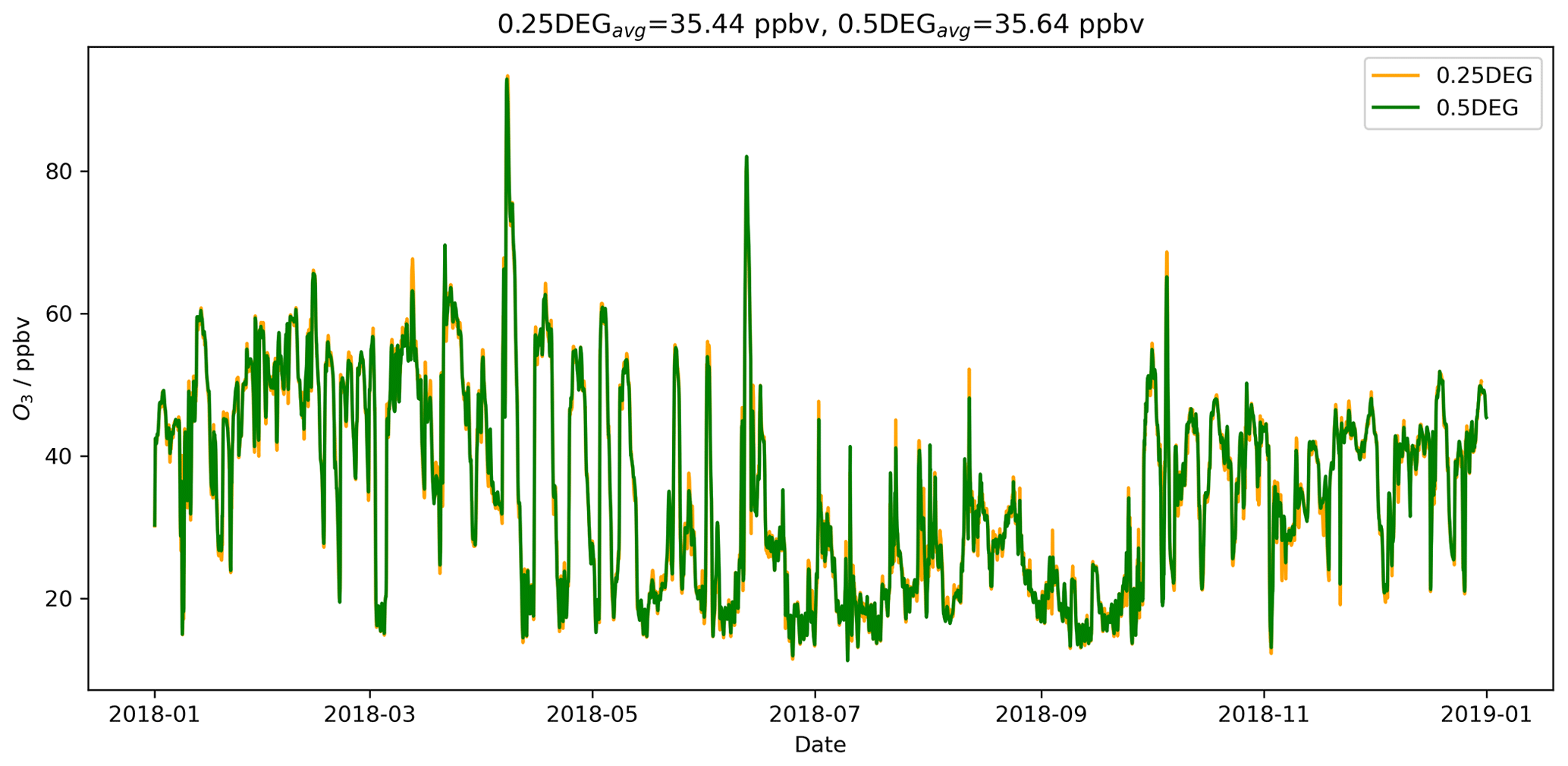
Figure A2 Modelled time series comparing O₃ simulation at 0.25^∘ × 0.3125^∘ and 0.5^∘ × 0.625^∘ resolution at the site.

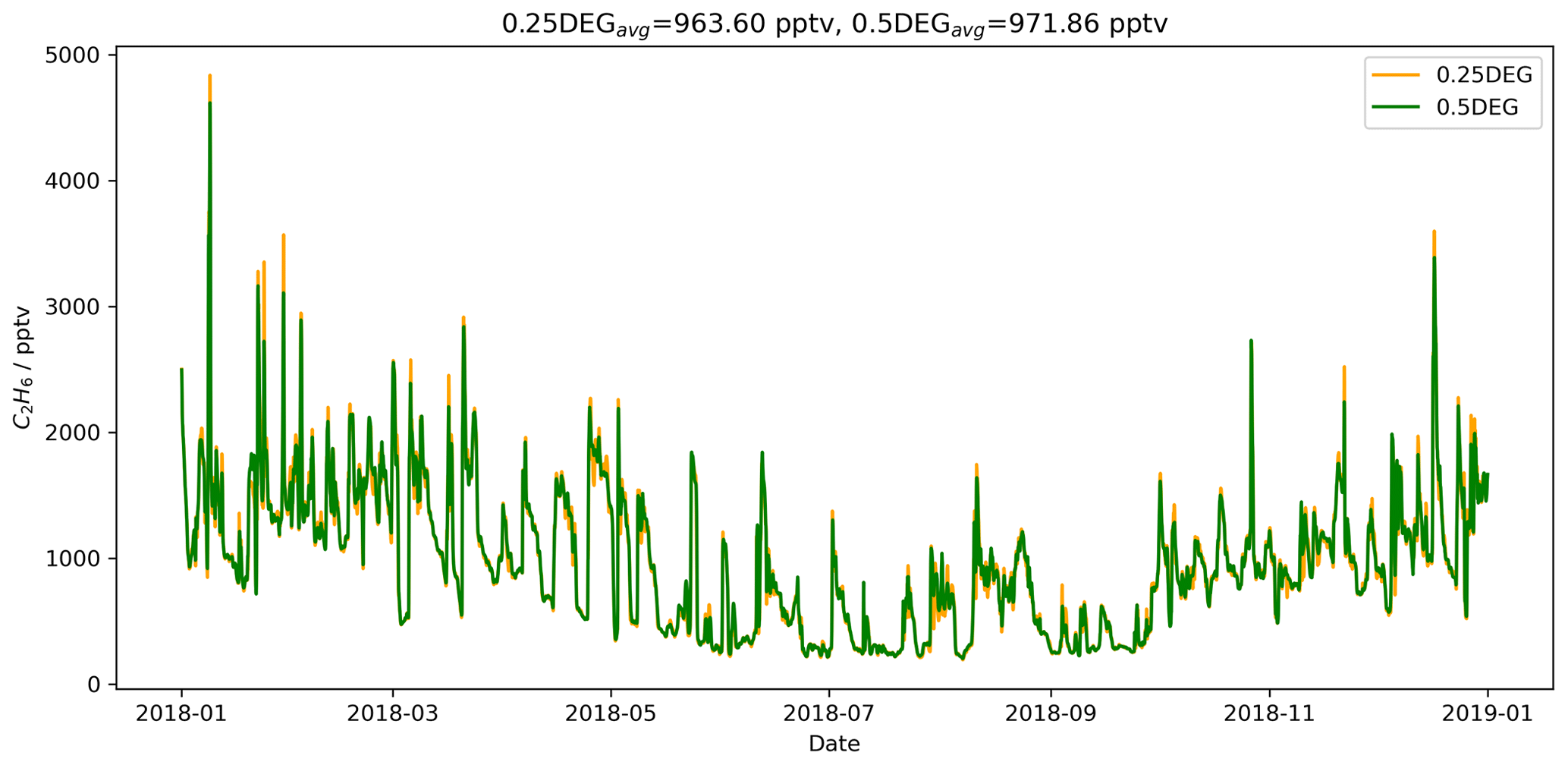
Figure A3 Modelled time series comparing C₂H₆ simulation at 0.25^∘ × 0.3125^∘ and 0.5^∘ × 0.625^∘ resolution at the site.

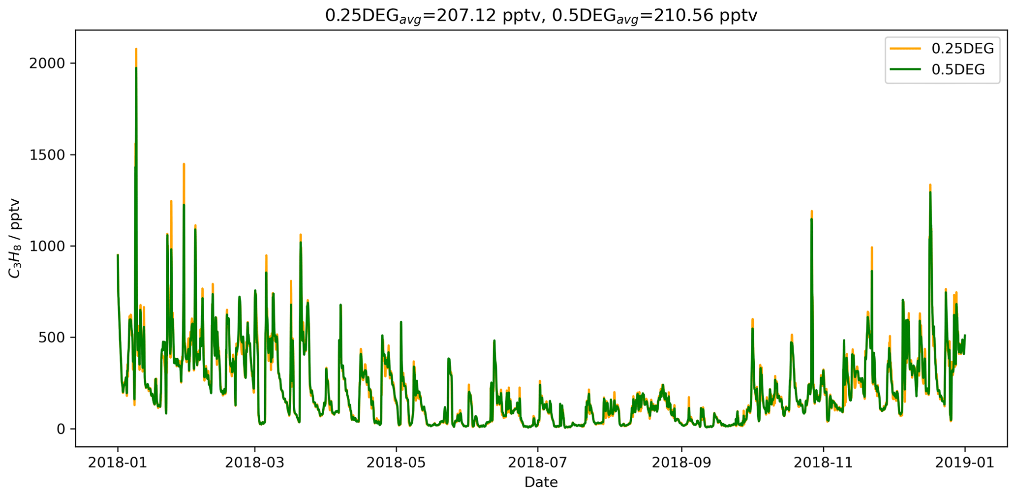
Figure A4 Modelled time series comparing C₃H₈ simulation at 0.25^∘ × 0.3125^∘ and 0.5^∘ × 0.625^∘ resolution at the site.

Appendix B: Other figures

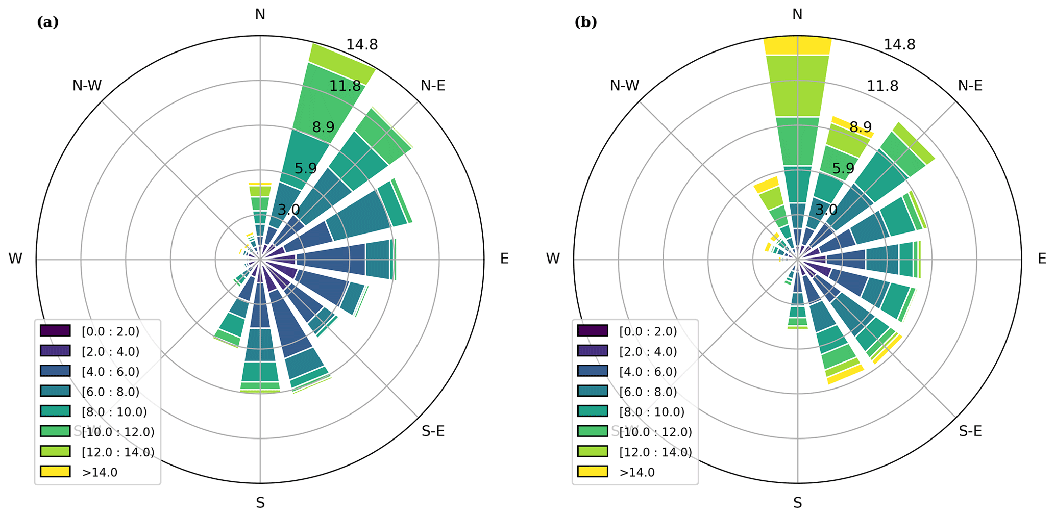
Figure B1 Wind rose for (a) observed and (b) modelled wind speed (m s⁻¹) and direction at Hateruma.

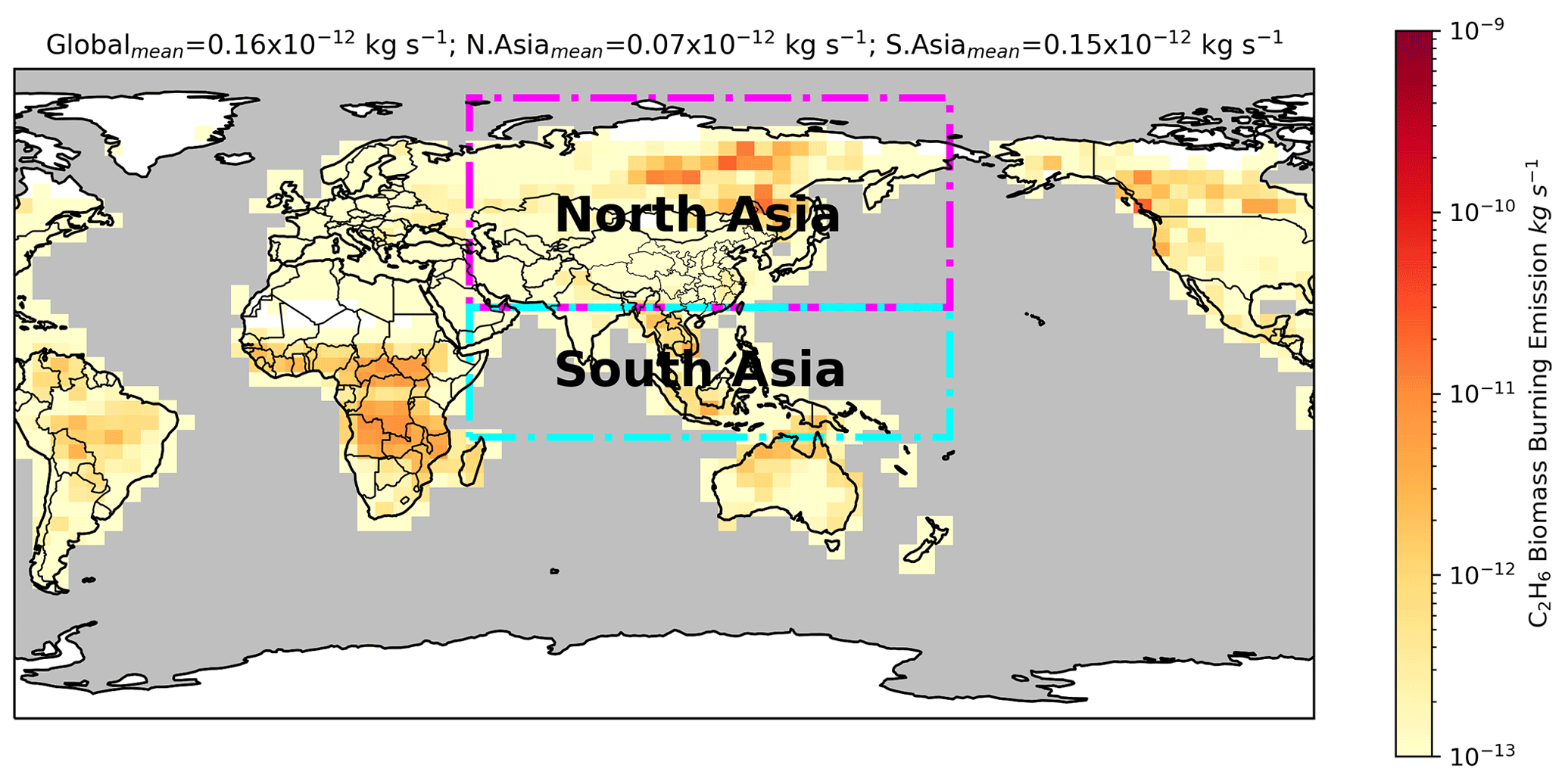
Figure B2 Annual mean biomass burning emission flux for C₂H₆ in 2018 (GFED). Regions indicated are the north and South Asia region, which had biomass burning emissions switched off in the simulations. The Asia box extends from 46 to 180^∘ E; north Asia box covers 82 to 24^∘ N, while South Asia spans −12 to 24^∘ N.

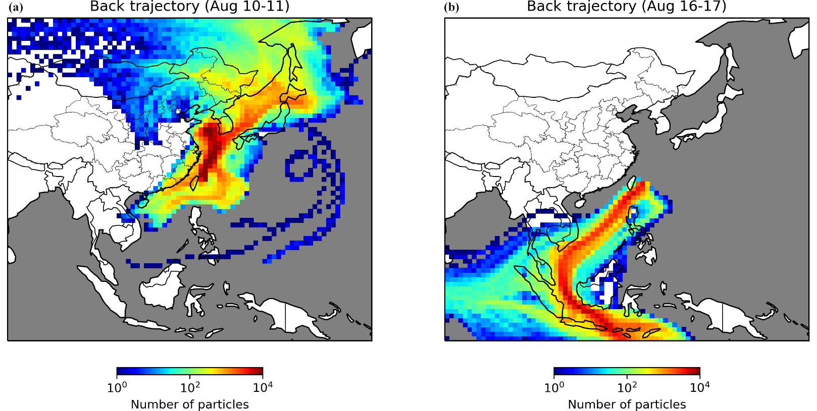
Figure B3 Back-trajectory analysis showing air masses arriving at Hateruma between (a) 10–11 August and (b) 16–17 August.