the Creative Commons Attribution 4.0 License.
the Creative Commons Attribution 4.0 License.
 | 21 Aug 2023
Sensitivity of northeastern US surface ozone predictions to the representation of atmospheric chemistry in the Community Regional Atmospheric Chemistry Multiphase Mechanism (CRACMMv1.0)
Bryan K. Place
William T. Hutzell
K. Wyat Appel
Sara Farrell
Lukas Valin
Benjamin N. Murphy
Karl M. Seltzer
Golam Sarwar
Christine Allen
Ivan R. Piletic
Emma L. D'Ambro
Emily Saunders
Heather Simon
Ana Torres-Vasquez
Jonathan Pleim
Rebecca H. Schwantes
Matthew M. Coggon
William R. Stockwell
Chemical mechanisms describe how emissions of gases and particles evolve in the atmosphere and are used within chemical transport models to evaluate past, current, and future air quality. Thus, a chemical mechanism must provide robust and accurate predictions of air pollutants if it is to be considered for use by regulatory bodies. In this work, we provide an initial evaluation of the Community Regional Atmospheric Chemistry Multiphase Mechanism (CRACMMv1.0) by assessing CRACMMv1.0 predictions of surface ozone (O3) across the northeastern US during the summer of 2018 within the Community Multiscale Air Quality (CMAQ) modeling system. CRACMMv1.0 O3 predictions of hourly and maximum daily 8 h average (MDA8) ozone were lower than those estimated by the Regional Atmospheric Chemistry Mechanism with aerosol module 6 (RACM2_ae6), which better matched surface network observations in the northeastern US (RACM2_ae6 mean bias of +4.2 ppb for all hours and +4.3 ppb for MDA8; CRACMMv1.0 mean bias of +2.1 ppb for all hours and +2.7 ppb for MDA8). Box model calculations combined with results from CMAQ emission reduction simulations indicated a high sensitivity of O3 to compounds with biogenic sources. In addition, these calculations indicated the differences between CRACMMv1.0 and RACM2_ae6 O3 predictions were largely explained by updates to the inorganic rate constants (reflecting the latest assessment values) and by updates to the representation of monoterpene chemistry. Updates to other reactive organic carbon systems between RACM2_ae6 and CRACMMv1.0 also affected ozone predictions and their sensitivity to emissions. Specifically, CRACMMv1.0 benzene, toluene, and xylene chemistry led to efficient NOx cycling such that CRACMMv1.0 predicted controlling aromatics reduces ozone without rural O3 disbenefits. In contrast, semivolatile and intermediate-volatility alkanes introduced in CRACMMv1.0 acted to suppress O3 formation across the regional background through the sequestration of nitrogen oxides (NOx) in organic nitrates. Overall, these analyses showed that the CRACMMv1.0 mechanism within the CMAQ model was able to reasonably simulate ozone concentrations in the northeastern US during the summer of 2018 with similar magnitude and diurnal variation as the current operational Carbon Bond (CB6r3_ae7) mechanism and good model performance compared to recent modeling studies in the literature.
- Article
(6260 KB) - Full-text XML
- Companion paper
-
Supplement
(4961 KB) - BibTeX
- EndNote


Both short-term acute and long-term chronic exposure to elevated surface ozone (O3) concentrations can be detrimental to human and ecosystem health (Bell et al., 2005; Rich et al., 2006; Larrieu et al., 2007; Iriti and Faoro, 2008; Ghosh et al., 2018; U.S. Environmental Protection Agency, 2020). The buildup of O3 in the lower atmosphere also has a noticeable impact on earth's radiative budget (e.g., Brasseur et al., 1998; Stevenson et al., 2013). As a result, many countries and governments across the world have enacted legislation to limit surface ozone pollution. In the United States the current National Ambient Air Quality Standards (NAAQS) for maximum daily 8 h average ozone (MDA8 O3) is set at 70 parts per billion by volume (ppb) (Bachmann, 2007; U.S. Environmental Protection Agency, 2015). Despite reductions in emissions of precursor gases that lead to O3 formation, many areas across the US are still in non-attainment of these standards (U.S. Environmental Protection Agency, 2022a). Thus, understanding current O3 pollution mitigation strategies and developing new strategies for the future are pivotal if air quality standards are to be met.
The chemistry of tropospheric O3 formation is complex and involves the non-linear reactions of nitrogen oxides (NOx = NO + NO2) with reactive organic carbon (ROC) compounds (Seinfeld and Pandis, 2006; Jacob, 1999; Heald and Kroll, 2020). Similarly, the formation of secondary fine-particle (PM2.5) species such as sulfate, nitrate, and secondary organic aerosol (SOA) involves complex chemistry in multiple phases and is dependent on concentrations of numerous precursor species and atmospheric oxidants. In total, this chemistry can involve thousands of individual chemical compounds and over 10 000 chemical reactions (Dodge, 2000; Stockwell et al., 2012; Jenkin et al., 2015). Due to these complex interactions as well as the role of meteorological and dry deposition processes on O3 and PM2.5 (Seinfeld and Pandis, 2006), regulatory bodies use numerical models to simulate past, current, and future (e.g., under modified emission scenarios) concentrations to inform air quality management. Rather than simulating the explicit chemistry of every known atmospheric compound and reaction, these models usually employ chemical mechanisms which simplify the atmospheric chemistry into a more limited number of species and reactions in order to capture the most important pathways for forming O3 and PM2.5 in a computationally efficient manner (Gery et al., 1989; Carter, 1990; Stockwell et al., 1997). Typically, the chemistry leading to O3 is represented separately from the chemistry leading to PM2.5 and SOA formation in chemical transport models (e.g., Pye et al., 2010; Koo et al., 2014).
The Community Multiscale Air Quality (CMAQ) model is a numerical model developed by the United States Environmental Protection Agency (U.S. EPA) to estimate O3, PM2.5, and other pollutants, both regionally in the US and in other parts of the world (http://www.epa.gov/cmaq, last access: 8 August 2023; U.S. Environmental Protection Agency, 2022b). CMAQ is available online (see “Code and data availability”) and is distributed publicly with three types of chemical mechanisms: the Regional Atmospheric Chemistry Mechanism (RACM), Carbon Bond (CB), and SAPRC. These three chemical mechanisms represent ozone chemistry with less than 1000 reactions and up to ∼ 200 species and have been tested on multiple model domains where they show acceptable performance at estimating ambient O3 concentrations (e.g., Sarwar et al., 2008, 2013; Yu et al., 2010; Mathur et al., 2017; Appel et al., 2021). Currently, Carbon Bond version 6 (CB6r3 as of CMAQv5.3) is the most common mechanism used by the U.S. EPA for predicting O3 (Appel et al., 2021).
The Community Regional Atmospheric Chemistry Multiphase Mechanism version 1.0 (CRACMMv1.0) (Pye et al., 2023) is a next-generation chemical mechanism that was distributed for the first time with the release of CMAQv5.4 in October 2022 (U.S. EPA Office of Research and Development, 2022). CRACMMv1.0 builds on the RACM2 framework (Goliff et al., 2013) and includes new representations of several organic systems, most notably monoterpenes and aromatics, and couples gas-phase with particle-phase products. In addition, the CRACMMv1.0 mechanism provides built-in transparent mapping of emissions to mechanism species and was designed to conserve emitted carbon as well as track carbon in products as gases react and evolve. These features were included in CRACMMv1.0 to represent particulate matter formation more accurately while also maintaining the ability to predict O3 concentrations.
The goal of this work is to compare CRACMMv1.0 O3 predictions with the previously well-established RACM2 and CB6r3 chemical mechanisms and understand drivers of differences between CRACMMv1.0 and these mechanisms. Future work will present analyses evaluating CRACMMv1.0 PM2.5 predictions. For the comparison presented here we used the CMAQ model and performed simulations at 4 km × 4 km horizontal grid resolution for the northeastern United States (US) domain during summer 2018 (Torres-Vazquez et al., 2022). This domain was chosen specifically because areas in the northeastern US frequently violate the O3 NAAQS (U.S. Environmental Protection Agency, 2022a). In addition, past field studies such as the Long Island Sound Tropospheric Ozone Study (LISTOS) and future field studies (e.g., Atmospheric Emissions and Reactions Observed from Megacities to Marine Areas, AEROMMA; Warneke et al., 2022) have been designed to specifically address the issue of high O3 events in the New York City metropolitan area. Air Quality System (AQS) observations made during the summer of 2018 were used to aid in the evaluation. Finally, a box model was employed to study the different chemical systems and updates that were driving differences in O3 predictions between RACM2 and CRACMMv1.0.
2.1 CMAQ model
CMAQ simulations were performed for the northeastern United States (NE US) domain at 4 km × 4 km horizontal grid resolution with 35 vertical layers from 1 June through 31 August 2018 with 2 through 31 May as the simulation spinup period. In addition to CRACMMv1.0, simulations were also performed with CB6r3 using aerosol module 7 (CB6r3_ae7; AERO7) (Appel et al., 2021) and with RACM2 using aerosol module 6 (RACM2_ae6; AERO6) (Sarwar et al., 2013), both of which are available in the standard CMAQv5.3.3 release (used here) and v5.4 (latest public release). The major difference between AERO6 and AERO7 is in the representation of monoterpene SOA, with AERO7 producing more monoterpene SOA from photooxidation (Xu et al., 2018) and organic nitrates (Pye et al., 2015) than AERO6. Chemical initial and boundary conditions for the NE US domain were generated from previous nested WRF-CMAQ simulations (Weather Research and Forecasting) (12 km), which used CB6r3_ae7 (Torres-Vazquez et al., 2022). The initial and boundary conditions from CB6r3_ae7 were mapped to CRACMMv1.0 and RACM2_ae6. See the CMAQv5.4 code repository for the mapping of Carbon Bond-based mechanisms to CRACMMv1.0 for boundary and initial condition purposes. Meteorological files for the simulation were generated offline using the Weather Research Forecasting (WRF version 4.1.2) model as described by Torres-Vazquez et al. (2022), and the files were pre-processed through the Meteorology-Chemistry Interface Processor (MCIP) (Otte and Pleim, 2010) for input to the CMAQ simulations.
2.2 Emissions
Anthropogenic emissions were created following the 2016 version 7.2 North American Emissions Modeling Platform (Torres-Vazquez et al., 2022; U.S. Environmental Protection Agency, 2019) with updates described below. The anthropogenic emissions for CB6r3_ae7 are the same as those for the 4 km domain in the work by Torres-Vazquez et al. (2022) and include year-specific mobile emissions predicted by the MOtor Vehicle Emission Simulator (MOVES) model, airport emissions following the 2017 National Emissions Inventory (NEI) estimates from the Federal Aviation Administration (FAA) airport model, year-specific wildland fires, monitored electric generating unit (EGU) emissions, year-specific commercial marine vehicle emissions, and emissions from other sectors following the 2016v7.2 modeling platform. Primary organic aerosol (POA) in CB6r3_ae7 was considered semivolatile, and evaporated POA was allowed to undergo gas-phase reaction with OH following the work of Murphy et al. (2017). The empirical representation of anthropogenic SOA sources (potential combustion SOA, pcSOA; Murphy et al., 2017) was turned off in all cases. For a more complete description of the anthropogenic emissions employed in the CB6r3_ae7 simulations, see the work by Torres-Vazquez et al. (2022). Biogenic emissions for all mechanism simulations were calculated within CMAQv5.3.3 using the EPA's Biogenic Emission Inventory System (BEIS v3.6.1) (Bash et al., 2016).
CRACMMv1.0 emission inputs build on the same methods as the CB6r3_ae7 inputs with a few additional updates. The total mass and speciation of emissions from volatile chemical products were updated to follow VCPy, a model for predicting volatile chemical product (VCP) emissions (Seltzer et al., 2021). Individual ROC species were mapped to CRACMMv1.0 species as described by Pye et al. (2023). Primary organic aerosol in CRACMMv1.0 was considered semivolatile with volatility profiles of alkane-like emissions for diesel vehicles, gasoline vehicles, and aircraft (Lu et al., 2020) and slightly oxygenated species profiles for biomass burning and all other POA sources. For sources without specific volatility profiles, the volatility profile of meat-cooking emissions was used to produce a lower bound on the evaporation of semivolatile species (Woody et al., 2016; Mohr et al., 2009). Semivolatile POA was implemented using the Detailed Emissions Scaling, Isolation, and Diagnostic (DESID) module in all cases (Murphy et al., 2021).
The anthropogenic emissions created for CRACMMv1.0 were also used with slight adjustments for RACM2_ae6 simulations in CMAQ (see Table S1 in the Supplement for mappings). For the RACM2_ae6 simulations, primary organic aerosol (POA) was treated as semivolatile with the same volatility profiles as in the CRACMMv1.0 simulations but with the chemistry of AERO6 (Murphy et al., 2017). Alkane-like semivolatile and intermediate-volatility organic compounds (S/IVOCs) emitted in the gas phase were ignored in RACM2_ae6, and the empirical representation of anthropogenic SOA sources (pcSOA, Murphy et al., 2017) was turned off in RACM2_ae6 as in CB6r3_ae7.
2.3 Air quality network observations
Surface-level network observations of air pollutants made in the northeastern US between June and August 2018 were used to evaluate CMAQ model outputs. Hourly measurements of O3 and NOx were obtained from the AQS database using the available pre-generated files and paired in time and space with model quantities using the Atmospheric Model Evaluation Tool (AMET) (Appel et al., 2011). The observations in AQS were quality-assured by the reporting agency (e.g., EPA, states, tribes), and therefore no additional quality checks of AQS data were done in AMET. In the case of time periods with missing data, those missing periods were removed from the analysis. In cases where multiple observations were reported for a single site using different parameter occurrence codes (POCs), those observations were treated as individual measurements with the POC number used to distinguish between the different measurements for the same site.
2.4 Box modeling in F0AM
The Framework for 0-D Atmospheric Modeling (F0AMv4.2) box model was used as a tool to examine differences in chemistry between the mechanisms (Wolfe et al., 2016). Chemical species and reactions from the RACM2 and CRACMMv1.0 mechanisms were ported into F0AM from CMAQ-ready mechanism files using a custom MATLAB script (see “Code and data availability”). Photolysis rates in RACM2 and CRACMMv1.0 were matched to existing Master Chemical Mechanism (MCM) rates in F0AM, and the F0AM default example actinic flux rates were prescribed for all simulations. Three chamber experiments were run by initiating experiments with 10 ppb of either α-pinene, isoprene, or benzene under high- (5 ppb) and low-NOx (0.5 ppb) conditions at standard temperature (T= 298 K) and pressure (P= 1013 mbar). Hydrogen peroxide, set at 200 ppb, was used as the radical OH source (∼ 2 × 10⁻⁴ ppb initial OH), and relative humidity was set at 10 % across all simulations. After initiation, each chemical system was allowed to evolve for 24 h to reach steady state before the simulation was terminated. In addition, to gain insight into the role organic vs. inorganic updates played in O3 production in CRACMMv1.0, all three ROC precursors were re-run in simulations using a modified RACM2 mechanism (RACM2_mod) where all inorganic rate constants in RACM2 were updated to match those in CRACMMv1.0. This was needed because the development of CRACMMv1.0 not only incorporated updates to various ROC reaction systems in terms of product yields and chemical fates but also included inorganic rate constant updates (> 20 rate constants) to reflect current literature values, which differ from those prescribed in RACM2.
3.1 Ozone predictions by mechanism
Figure 1a shows the June–August average surface ozone concentration (averaged for all hours) predicted by the CRACMMv1.0 chemical mechanism across the northeastern US model domain. CRACMMv1.0 average ozone predictions ranged from 16–32 parts per billion by volume (ppb), with the highest average ozone predictions occurring over the Great Lakes region, Appalachian Mountain region, and the Atlantic coastline. The higher average O3 predictions (28–32 ppb) in the Great Lakes region and around Chesapeake Bay (Fig. 1) have been shown to be driven by land–water circulation due to the difference in daytime planetary boundary layer (PBL) heights over cool water (typically < 300 m) compared to much higher PBL heights over land (often 1500–2500 m) (Dye et al., 1995; Lennartson and Schwartz, 2002; Foley et al., 2011; Dreessen et al., 2019; Cleary et al., 2022). In particular, O3 exceedance events around Lake Michigan have been predominantly attributed to the northeasterly transport of O3 and O3 precursors to the lake, where photochemical O3 production then becomes intensified under conditions of lower vertical mixing and lower dry deposition (Sillman et al., 1993; Dye et al., 1995; Lennartson and Schwartz, 2002; Foley et al., 2011; Cleary et al., 2022). These lake effects often lead to regular NAAQS exceedances in the region (Foley et al., 2011). The elevated O3 concentrations predicted for the Appalachian Mountain region have also been shown to be driven primarily by the transport of O3 and other pollutants from nearby urban centers and coal-fired power plants (Aneja et al., 1991; Neufeld et al., 2019). In addition, O3 losses in the region have been measured to be lower at the higher elevation on the mountaintops, which leads to the buildup of O3 during the night (Aneja et al., 1991; Neufeld et al., 2019).
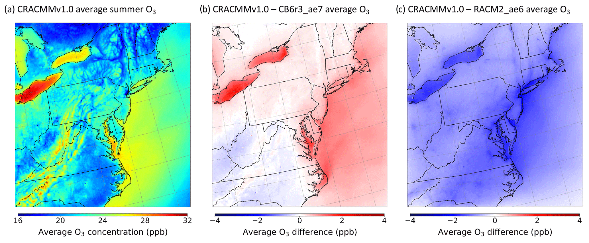
Figure 1(a) Simulated summer (June–August) 2018 surface ozone average (all hours) as predicted by CRACMMv1.0. Simulated summer ozone average (all hours) differences of (b) CRACMMv1.0 − CB6r3_ae7 and (c) CRACMMv1.0 − RACM2_ae6.
The magnitude of the ozone concentrations predicted by CRACMMv1.0 was in good agreement with O3 predictions from the base CB6r3_ae7 simulation, with inland differences typically falling below ±1 ppb across the model domain (Fig. 1b). These absolute differences corresponded to relative differences of ±5 % (Fig. S1a). The largest observed spatial discrepancies between the two mechanisms occurred near bodies of water, where CRACMMv1.0-estimated average ozone was ∼ 2–4 ppb higher than estimates made by the CB6r3_ae7 chemical mechanism. The higher predicted differences near water are likely explained by intensified chemistry due to the land–water circulation effect described previously, which generally drives the higher O3 concentrations in the regions. In addition, Foley et al. (2011) and Vermeuel et al. (2019) found that O3 production showed greater NOx sensitivity as urban plumes advected across Lake Michigan. Thus, differences in O3 production near waterbodies between the simulations were influenced by the representation of O3–NOx–ROC chemistry in the two mechanisms and their characterization of the chemical regime. Differences in chemical production of O3 between CRACMMv1.0 and CB6r3_ae7 are discussed and further explored later (Sect. 4.2). The differences over water between CB6r3_ae7 and CRACMMv1.0 were not expected to be driven by dry deposition over the Great Lakes as deposition is largely suppressed over water (Sillman et al., 1993).
Because different VCP emission inventories were employed between the CRACMMv1.0 and CB6r3_ae7 simulations (see Sect. 2.2), differences in the two inventory methods, in addition to differences in chemistry, could account for a small fraction of the differences shown in Fig. 1b. This would be expected to have the most pronounced effect over urban areas, where VCP emissions are largest. In a previous model study, simulations showed that a complete removal of VCP emissions led to a 1 ppb O3 change in downtown New York City over a 24 h period (Seltzer et al., 2022); thus, the choice of VCP inventory is expected to result in differences much less than 1 ppb.
In comparison with RACM2_ae6, CRACMMv1.0 estimated a lower average concentration (average O3 difference of 2–4 ppb) across the model domain, with the largest differences in predictions occurring near urban centers in the metropolitan northeastern US in addition to coastal areas along the Great Lakes region and the Atlantic seaboard (Fig. 1c). The mechanism-to-mechanism average O3 differences presented in Fig. 1c corresponded to relative average O3 differences of 0 %–15 % between the mechanisms across the model domain (Fig. S1b). The coupling of meteorology and chemistry, similar to the situation discussed for Lake Michigan, could again explain the larger relative differences in O3 concentrations near waterbodies (Fig. 1c). Since RACM2_ae6 emissions were mapped from CRACMMv1.0 inputs, the differences between these simulations were due to chemical differences between the mechanisms alone. Over land, differences in O3 predictions between CRACMMv1.0 and RACM2_ae6 were smaller (< 2 ppb, < 7 %) but were consistently biased in one direction (Figs. 1c, S1b). These findings suggest that updates in chemistry between RACM2_ae6 and CRACMMv1.0 led to a ubiquitous reduction in O3 across the model domain. The role of chemistry as a driver in mechanism-to-mechanism ozone differences between RACM2_ae6 and CRACMMv1.0 is revisited in Sect. 4.
3.2 Evaluation of spatial distribution
Hourly ozone performance statistics were calculated by pairing CMAQ outputs in space and time with 313 AQS sites that reported hourly observations between the months of June and August 2018 using AMET (See Sect. 2.3). Figure 2a and b show the spatial distribution in model–observation hourly mean biases and linear correlations (r) between predictions and observations for all hourly observations covered by the CRACMMv1.0 simulation. In general, the hourly O3 mean bias (MB) indicates a high bias across the model domain, with the highest biases (> 15 ppb) occurring along the North Carolina–Tennessee border (Fig. 2a). Model biases were much lower around the metropolitan NE US (Washington, DC; Maryland; New Jersey; New York City–Long Island regions), where predictions fell within ±4 ppb of the observed average values. Linear correlations between hourly O3 estimates and observations at a given AQS site were typically high (r > 0.8) in the northeastern US (Fig. 2b). Correlations between hourly observations and predictions were the weakest at sites located in the Appalachian Mountain region (r= 0.4–0.6) and were strongest at sites located in the metropolitan northeastern US (r > 0.9). The hourly O3 normalized mean bias (NMB) and normalized mean error (NME) across the domain can be found in the Supplement (Fig. S2), and values followed a similar spatial distribution as Fig. 2a and b, with lower NMB (−20 % to +20 %) and NME (< 30 %) values nearer population centers (e.g., Washington, DC; Baltimore; Philadelphia; Boston) and higher NMB (+ 20 %–100 %) and NME (> 40 %) at sites further from city centers (Fig. S2). Even so, hourly ozone predictions had values of NMB between ±20 % at 250 out of 313 sites and NME less than 30 % at 227 out of 313 of the reporting sites.
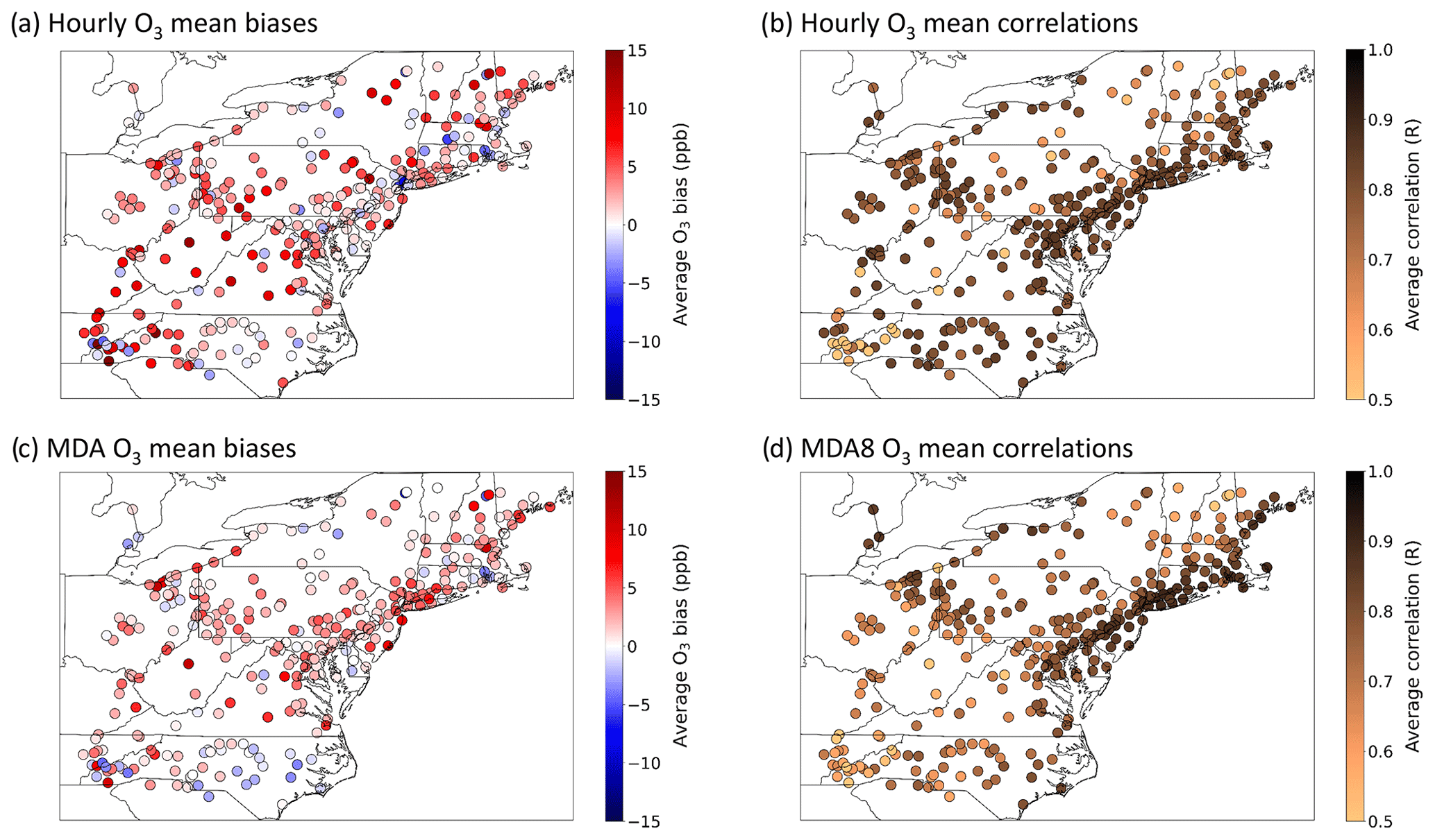
Figure 2Ozone (a, c) mean biases (in ppb) and (b, d) correlations between predictions and observations for (a–b) all hourly O3 values and (c–d) MDA8 O3 values across the NE US for CRACMMv1.0 calculated using AQS observations between June–August 2018.
The bias and correlation for daily maximum 8 h average ozone concentration (MDA8 O3) were also calculated for CRACMMv1.0 at each site (Fig. 2c, d). Predictions of MDA8 O3 are often used by regulating bodies, such as the U.S. EPA, to determine whether regions are in attainment or non-attainment of national ozone air quality standards. Predictions of MDA8 O3 also reflect a model's ability to estimate daytime O3 concentrations as O3 concentrations are higher during the day. CRACMMv1.0 MDA8 O3 mean biases were similar to the reported hourly O3 biases and ranged from −4 to +16 ppb across the model domain, with model–observation biases falling within ±4 ppb at 245 out of 313 sites (Fig. 2c). Correlations between modeled and observed MDA8 O3 were also determined to be high (Fig. 2d), and CRACMMv1.0 MDA8 O3 predictions showed a stronger correlation than hourly O3 predictions at the Appalachian Mountain sites (e.g., North Carolina–Tennessee border) but were weaker in central North Carolina and in Ohio. MDA8 O3 normalized mean biases did not exceed ±40 %, with 305 sites reporting normalized mean biases within ±20 % (Fig. S2c). MDA8 O3 normalized mean errors did not exceed 45 % across the domain, and NME values were lower than 20 % for the majority (95 %) of sites (Fig. S2d).
Hourly and MDA8 O3 predictions that were biased high were not isolated to the CRACMMv1.0 simulation as both the CB6r3_ae7 and RACM2_ae6 hourly and MDA8 O3 estimates showed high biases over the northeastern US in summer 2018 (Figs. S3–S6). High summer O3 daytime and nighttime biases have been noted in previous studies in CMAQ investigating air quality over the northeastern US and contiguous US (CONUS) using the RACM2 and CB6 mechanisms (Appel et al., 2021; Sarwar et al., 2013; Cheng et al., 2022). Cheng et al. (2022) noted in their study that daytime high O3 biases were reduced by a more accurate representation of cloud cover via the assimilation of satellite data. Nighttime overestimation of O3 in a previous study using CMAQ, on the other hand, was attributed to high O3 coming in from the domain boundaries and low vertical mixing (Li and Rappenglueck, 2018). The exact drivers of the high summer O3 estimates in CMAQ, however, are still under investigation. The calculated hourly and MDA8 ozone statistics for the CB6r3_ae7 and RACM2_ae6 simulations were found to be of very similar spatial distribution and magnitude to those calculated for CRACMMv1.0 (Figs. 2 and S2–S6), where both simulations reported lower biases in the metropolitan NE US and higher biases in other areas of the domain. Given that all mechanism O3 biases were lowest nearer to major cities, this suggests that the CMAQ simulations better estimated O3 concentrations in areas exposed to higher levels of anthropogenic pollutants.
Table 1 summarizes the domain-wide averages of site-specific ozone performance statistics for all three mechanisms and highlights that CRACMMv1.0 performed well when compared with domain-wide hourly and MDA8 O3 estimates from RACM2_ae6 and CB6r3_ae7. The lower O3 estimates by CB6r3_ae7 across the domain most closely matched observations and showed the lowest domain-wide hourly and MDA8 O3 mean bias (MB), normalized mean bias (NMB), and normalized mean error (NME). CRACMMv1.0 hourly O3 predictions showed a similar MB (+2.7 ppb vs. +2.4 ppb) and NMB (+8.8 % vs. +7.9 %) to CB6r3_ae7, while CRACMMv1.0 MDA8 O3 MB (+2.1 ppb vs. +1.5 ppb) and NMB (+7.7 % vs. +3.4 %) values were slightly higher than CB6r3_ae7.
While on average, hourly O3 and MDA8 O3 were slightly overestimated by all mechanisms, the highest O3 values were generally underestimated by all mechanisms (Table 1). For the subset of conditions where observed O3 was above 50 ppb (approximately the highest 10 % of concentrations) RACM2_ae6 (MB of −1.7 ppb) performed best followed by CRACMMv1.0 (MB of −4.7 ppb) and then CB6r3_ae7 (MB of −6.2 ppb). CRACMMv1.0 with the Automated MOdel REduction (AMORE) representation of isoprene chemistry (CRACMM1AMORE) is expected to perform even better than CRACMMv1.0 at high ozone concentrations (Wiser et al., 2022).
Table 1Performance of domain-wide site-specific average hourly O3 (number of observations, n= 652 476), MDA8 O3 (n= 27 037), and hourly O3 above 50 ppb (n= 69 103) in terms of mean bias (MB), the Pearson correlation coefficient (r), normalized mean bias (NMB), and normalized mean error (NME) for the CRACMMv1.0, and CB6r3_ae7, and RACM2_ae6 simulations. The last rows reflect conditions when observed hourly ozone was above 50 ppb.
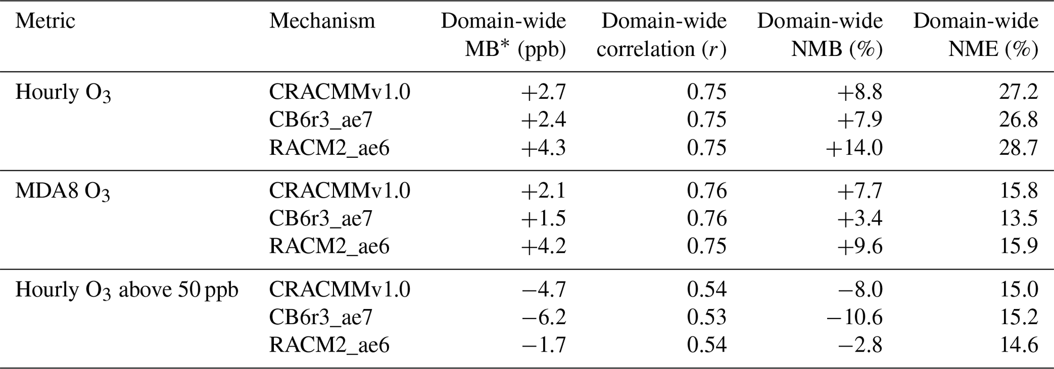
* Equations used for the calculations of MB, r, NMB, and NME are reported in the Supplement.
Emery et al. (2017) characterized NMB and NME model statistics from modeling studies reported in the literature (Simon et al., 2012) and found that two-thirds of modeling studies reported hourly and MDA8 NMB of <15 %, NME of <25 %, and r of >0.50. With the exception of domain-wide hourly O3 NME, all mechanisms examined here had model performance (NMB, NME, and r) within the range reported in the literature. By these metrics, CRACMMv1.0 performs consistently with state-of-science criteria for predicting O3 in photochemical models while also treating the loss of mass to SOA formation.
3.3 Evaluation of diurnal distribution
Figure 3a shows the diurnal average hourly ozone surface concentrations (±1 standard deviation) estimated by CRACMMv1.0 (blue trace) compared to average hourly network observations (±1 standard deviation) for all AQS sites (black trace) that reported measurements during the summer of 2018 within the domain. Figure 3a shows that CRACMMv1.0 captured the general diurnal pattern of the observed ozone concentrations across the model domain, and predictions fell within the standard deviation of the observations. CMAQ simulations using CRACMMv1.0 predicted a similar onset in O3 production and an earlier and sharper decline in afternoon O3 than what was typically observed at the AQS sites. The model also predicted higher average nighttime minimum O3 than what was observed. The average summer diurnal O3 concentrations predicted by CMAQ using the CB6r3_ae7 (dashed red trace) and RACM2_ae6 (dashed green trace) mechanisms followed the same diurnal trend, with CRACMMv1.0 and CB6r3_ae7 simulations showing better agreement with hourly observations than the RACM2_ae6 simulation (Fig. 3a).
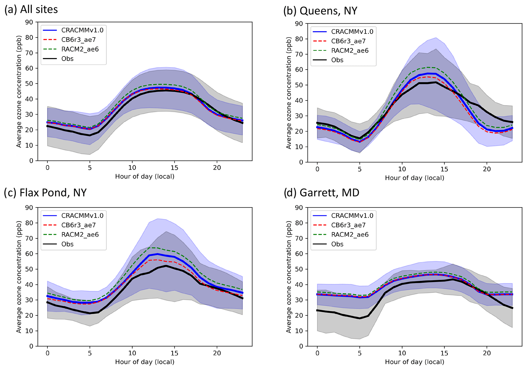
Figure 3Average (± standard deviation) hourly O3 concentrations predicted by CMAQ using CRACMMv1.0 (blue trace) and observed (black trace) at (a) all AQS sites within the domain; (b) Queens, NY (AQS site 36-081-0124); (c) Flax Pond, NY (AQS site 36-103-0044); and (d) Garrett, MD (AQS site 24-023-0002) during June, July, and August 2018. Predicted average hourly O3 values in the CB6r3_ae7 CMAQ simulation (dashed red trace) and the RACM2_ae6 CMAQ simulation (dashed green trace) are also overlaid in each panel.
Because the offset observed in morning growth and late-afternoon decline in O3 between CMAQ and the AQS observations was predicted by all mechanism simulations, meteorology was likely a driving contributor to the model–observation discrepancies during these time periods. For example, a previous study comparing CMAQ O3 predictions across North America determined that the timing of the diurnal ozone signal was likely driven by boundary layer dynamics in the model over emissions or chemistry (Solazzo et al., 2017). As mentioned in Sect. 3.2 the high nighttime biases observed in Fig. 3a could have also been driven by meteorology or by O3 coming in from the boundaries (Li and Rappenglueck, 2018). However, mechanism-to-mechanism differences and, more specifically, predictions of peak O3 during the daytime are influenced by the different treatments of chemistry between the simulations.
To further examine how different treatments of chemistry and/or emissions impacted hourly O3 differences between mechanisms compared to observations, comparisons at three selected AQS sites (one urban, one suburban, and one rural site) were also plotted in Fig. 3b, c, and d. Queens, NY, was chosen as a representative urban site (average hourly [NOx]mod ≈ 12 ppb); Flax Pond, NY, was chosen as a representative suburban site (average hourly [NOx]mod≈ 3 ppb); and Garrett, MD, was chosen as a representative rural/remote site (average hourly [NOx]mod < 1 ppb). Similar to Fig. 3a, all mechanism predictions fell within the standard deviation of the observations at all hours for all three sites (Fig. 3b, c, d). The RACM2_ae6 simulation showed the greatest diurnal change in hourly O3 concentrations (daytime ozone production) and highest daytime biases, while CB6r3_ae7 predicted the smallest changes in hourly O3 (daytime ozone production) and showed the lowest daytime biases at all three sites. All simulations showed the lowest hourly relative biases (±10 %) at the urban site (Queens, NY), suggesting that the model provides reasonable prediction of O3 production under high-NOx conditions. This reduced bias in an urban area is consistent with the hourly O3 biases shown previously across the northeastern US (Figs. 2 and S2–S6), where spatial biases were found to be lowest in the metropolitan NE US where local ozone formation is expected to make up a larger fraction of total ozone than at more rural locations. Larger differences between hourly mechanism-to-mechanism O3 predictions were observed at the more polluted sites. In particular, the daytime O3 estimated by RACM2_ae6 at Queens and Flax Pond (Fig. 3b, c) showed a much larger relative increase to CRACMMv1.0 and CB6r3_ae7 than what was seen at Garrett, MD (Fig. 3d). Again, this may in part be due to larger relative contribution from boundary conditions and transported ozone at rural locations vs. urban locations. Modeled NOx concentrations at all the sites were similar between mechanisms (within ±0.05 ppb), and the relationship between ozone production and NOx is further explored in the following section.
In this section, CMAQ simulations with emission perturbations are combined with box modeling to understand drivers of ozone formation. In addition, mechanism ozone production efficiency is quantified using modeled NOx and O3 concentrations across the northeastern US.
4.1 Sensitivity to specific ROC emissions
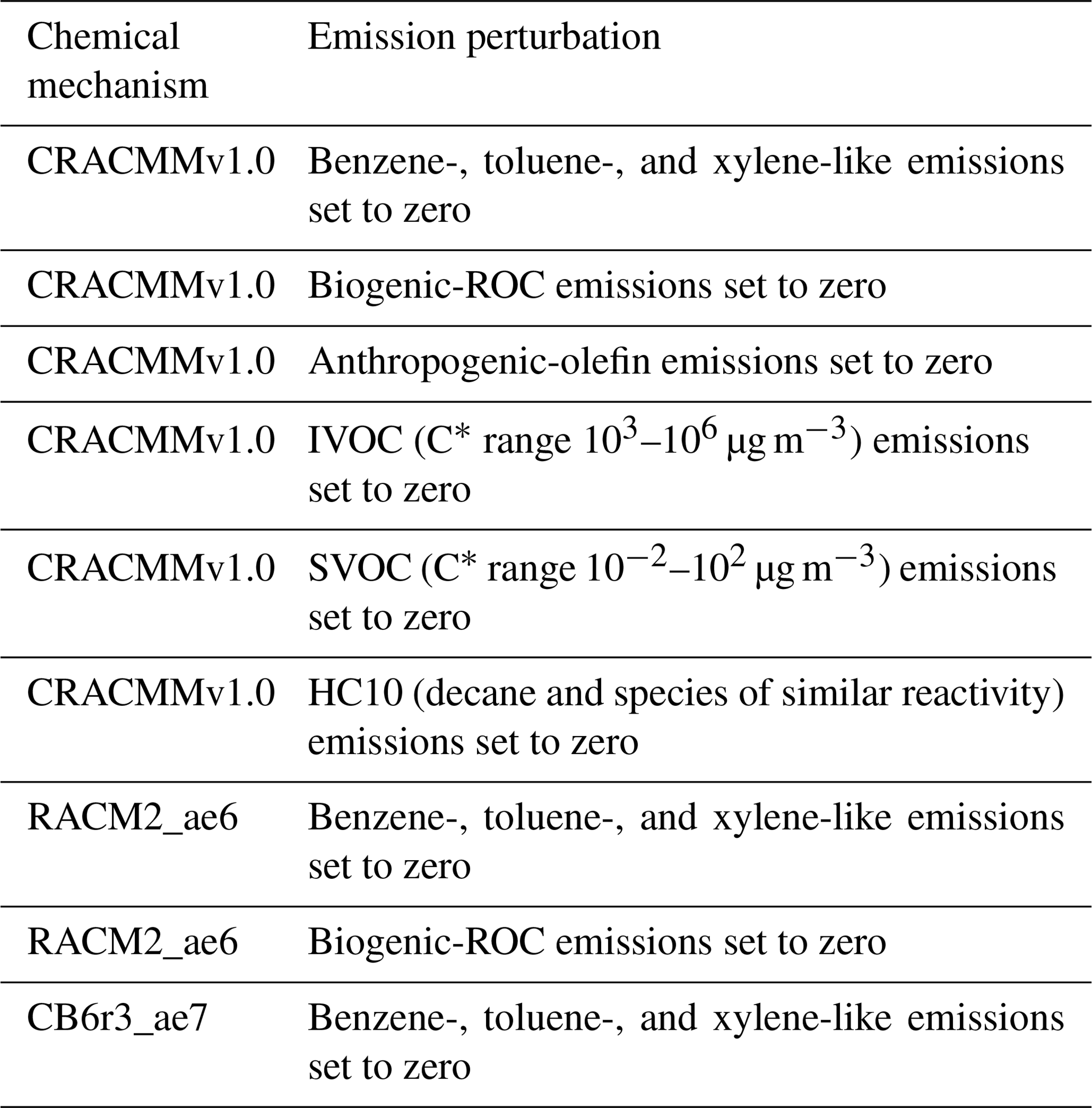
A series of emission sensitivity simulations were performed in CMAQ to gain insight into the precursor ROC systems important for O3 formation in CRACMMv1.0 across the NE US summer 2018 model domain. The sensitivity simulations were conducted by running a set of zeroed emission simulations (i.e., setting emissions of a chemical class or emission sector to zero) and determining the response in O3 concentrations to the emission perturbation. A list of all the zeroed emission simulations can be found in Table 2. Due to the non-linear response of ozone production to perturbations in NOx concentrations, the interpretations of zeroed emission simulations can be challenging. Nonetheless, these types of perturbations provide an initial assessment of the ozone production response in CRACMMv1.0 and provide insight into how chemical systems respond to lower ROC emissions in CRACMMv1.0 vs. RACM2_ae6 and CB6r3_ae7. Figure 4 shows domain-wide percent differences in average ozone concentrations (ΔO3) between the base CRACMMv1.0 simulation and a series of zeroed emission simulations. The largest ΔO3 response occurred when emissions from biogenic sources were excluded from the simulation (Fig. 4a). The zeroed biogenic-emission simulation resulted in percent changes in average O3 concentrations ranging from −10 % to +3 %. Spatially, average O3 concentrations decreased by ∼ 5 %–10 % in the metropolitan northeastern US and increased in the southern part of the model domain in response to the perturbation. Relatively large changes in ΔO3 were also predicted in the zeroed olefin and benzene–toluene–xylene (BTX) emission simulations, with average O3 concentration changes ranging from −4 % to +2 % (Fig. 4b, c). A similar spatial response in ΔO3 was seen between the zeroed biogenic-emission and anthropogenic-olefin emission simulations (Fig. 4a, b), while the response of ΔO3 in the zeroed BTX emission simulation was localized to urban areas, particularly in the metropolitan NE US and never indicated disbenefits (Fig. 4c). The chemical formation of O3 in CRACMMv1.0 was less sensitive to large alkanes (HC10) and semivolatile and intermediate-volatility organic compound (S/IVOC) emissions across the model domain as a ΔO3 response of +1 % was predicted in these simulations (Fig. 4d, e). All five sensitivity simulations showed some reduction in O3 in the New York City urban core with ROC reductions indicating ROC-sensitive ozone formation.
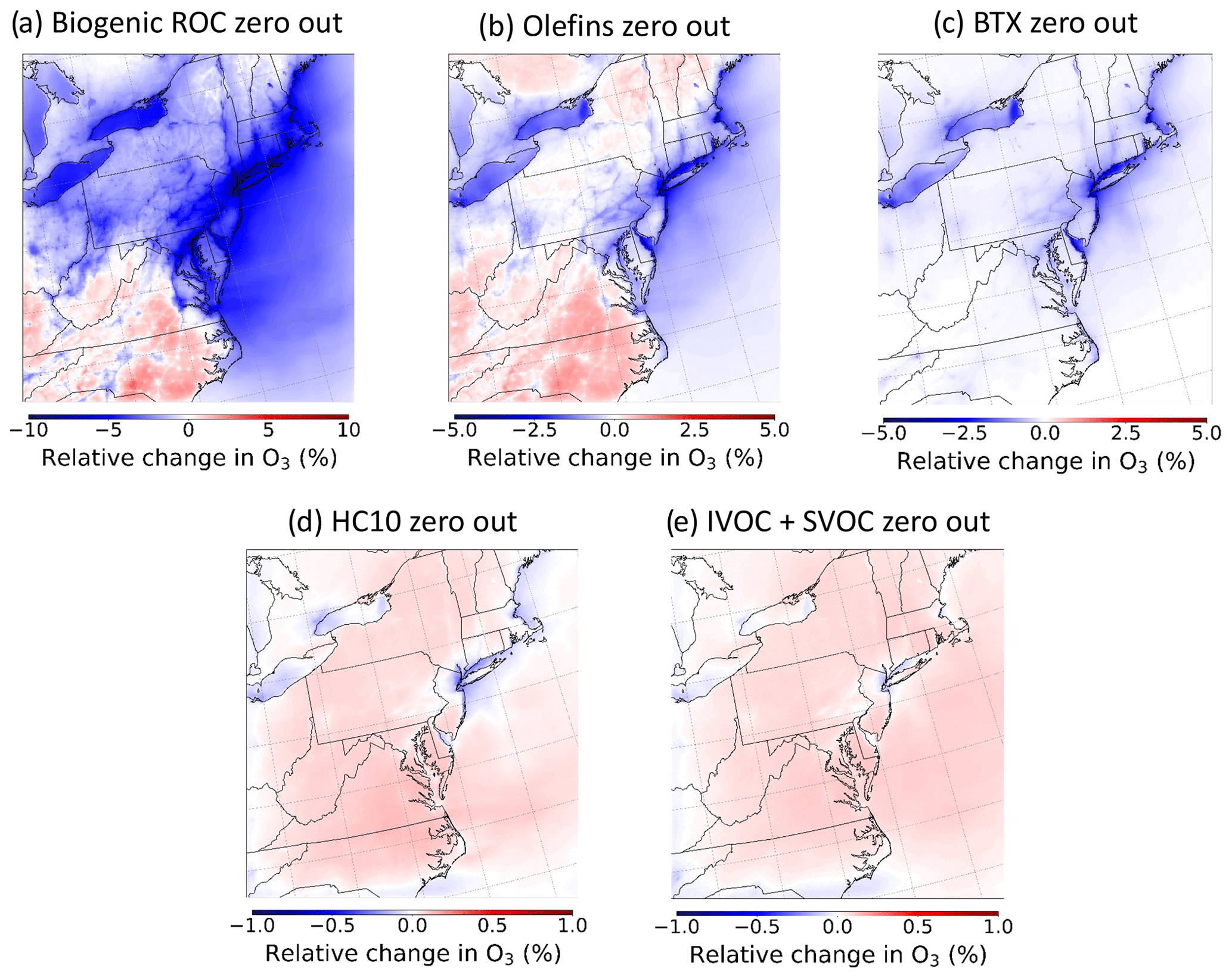
Figure 4Relative changes in O3 concentrations from the CRACMMv1.0 base simulation (zeroed emissions − base) for the (a) zeroed biogenic-emission scenario, (b) zeroed olefin emission scenario, (c) zeroed BTX emission scenario, (d) zeroed HC10 emission scenario, and (e) zeroed S/IVOC emission scenario.
Table 2List of emission perturbations relative to the base simulations in CMAQ. In the case of IVOC and SVOC emission perturbations, species over a saturation concentration, C*, range are modified.
A ΔO3 response like the one in CRACMMv1.0 was also predicted when biogenic emissions were zeroed in a simulation run with RACM2_ae6 (+3 % to −10 %) (Fig. S7), indicating that biogenic emissions were important to O3 formation across chemical mechanisms in the northeastern US domain. This strong sensitivity of O3 formation to biogenic-ROC emissions in the eastern and northeastern United States has also been noted in previous chemical transport model studies (e.g., Hogrefe et al., 2004; Fiore et al., 2005). A slightly higher and more widespread decrease in ΔO3 was seen in the RACM2_ae6 zeroed biogenic-emission simulation (Fig. S7) than in the CRACMMv1.0 zeroed emission simulation (Fig. 4a), which suggests different representations of biogenic-ROC chemistry between CRACMMv1.0 and RACM2_ae6 lead to some of the differences in modeled O3 concentration shown in Figs. 2 and 4. Zeroed BTX emission simulations run using RACM2_ae6 and CB6r3_ae7 (Figs. S8 and S9) resulted in ΔO3 responses (−2 % to −4 %) around urban areas similar to those that were observed in the CRACMMv1.0 zeroed BTX emission simulation (Fig. 4c). Domain-wide BTX emission effects on ozone were lower than biogenic-emission effects and more pronounced in urban source regions. Unlike CRACMMv1.0, the RACM2_ae6 and CB6r3_ae7 simulations predicted slightly higher ozone concentrations (ΔO3 = +1 %) in non-urban regions in the domain in the zeroed BTX emission simulations compared to the base model run (Figs. S8 and S9). Note that the organic nitrate yield in aromatic systems was reduced from 8.2 % to 0.2 % based on recent work by Xu et al. (2020) in CRACMMv1.0 (Pye et al., 2023). This change increases NO-to-NO2 conversion, which indicates BTX oxidation generally leads to ozone production in CRACMMv1.0. However, CRACMMv1.0 also removes radicals from the gas phase when autoxidation or phenol chemistry leads to SOA, thus reducing radical abundances, and Sect. 4.2 will illustrate that CRACMMv1.0 has a different baseline O3 prediction than RACM2_ae6 for benzene. These results indicate that the differing representation of aromatic chemical systems within the mechanisms explains some of the differences in modeled O3 concentrations shown in Sect. 3.
The modeled reductions in O3 seen near urban regions (Fig. 4a–c) and in the New York City urban core specifically (Fig. 4a–e) are mechanistically consistent for regions expected to have relatively high emissions of NOx, and thus reductions in ROC would lead to less ozone production. In these more ROC-sensitive regions, ozone production drops due to changes in total ROC reactivity. When ROC emission reductions are large enough (such as in the zeroed biogenic-ROC emission simulation in Fig. 4a), even NOx-sensitive locations could transition to a NOx-saturated chemical regime, where ROC reductions reduce ozone. The zeroed emission simulations often showed less sensitivity in the ΔO3 response to emission reductions in rural/remote regions (Fig. 4a–c) and even predicted an increase in O3 formation in rural regions in response to some emission perturbations (Fig. 4a, b, d, e). S/IVOCs and large alkanes (HC10) in particular suppressed ozone formation in the base simulation as indicated by their zeroed emission simulations, leading to increases in ozone with the exception of the New York City urban core (Fig. 4d, e). The ozone formation potential for HC10 compounds across the entire US for all of 2017 was high in previous work due to the overall abundance of emissions despite low maximum incremental reactivity (MIR) (Pye et al., 2023); however a much smaller change in average O3 concentration (±1 %) was observed in the zeroed HC10 emission simulation here compared to the olefin and BTX simulations. This result suggests that the emissions of HC10 compounds were relatively less important to ozone formation in the NE US domain compared to the entire US for all of 2017. Given the low MIR of IVOC and SVOC compounds, zeroing the emissions of these compounds was expected to have mild impacts on O3 formation, and Fig. 4e showed that O3 concentrations increased by ∼ 0.5 % across the full domain.
The emission perturbation results suggest that large volatile alkanes (HC10 and S/IVOCs) primarily act to sequester oxidants such as OH and NOx, thus resulting in increases in O3 for the zeroed emission simulations. Specifically, S/IVOC alkanes as well as HC10 in CRACMMv1.0 sequester NOx with the high efficiency due to a 26 %–28 % yield of alkyl nitrates (Pye et al., 2023). This hypothesis is supported by observed domain-wide increases (up to 4 %) in NO2 when both HC10 and SVOC emissions are removed from the simulations (Figs. S10 and S11). In addition, organic nitrates decrease up to 10 % near the urban core when HC10 emissions are omitted from the simulation (Fig. S12). Decreases in organic nitrate formation due to emission removal could also explain the increases in O3 formation seen in the rural regions of the zeroed biogenic-emission and olefin emission simulations (Fig. 4a, b), where O3 formation would increase in response to less NOx loss in a NOx-sensitive regime.
4.2 Ozone production efficiency
Ozone production efficiency (OPE) is defined as the number of molecules of O3 produced per molecule of NOx loss and can be viewed as a metric describing chain length in O3 propagation before NOx is chemically removed from the atmosphere (Jacob, 1999). Thus, model-constrained OPE estimates can provide mechanistic insight into O3–NOx–ROC cycling within a given chemical system or region. Operationally, OPE has been calculated using the slope of the linear regression between O3 and the sum of all NOx oxidation products (NOz) as O3 and NOz evolve during the photochemically active hours of the day (e.g., Arnold et al., 2003; Sarwar et al., 2013; Henneman et al., 2017). This OPE proxy (ΔO3 NOz) provides a good first-order approximation of OPE but may not sufficiently capture ozone recycling in regions impacted by fresh NOx emissions and regions where NOx and NOz losses through deposition are high. Using this proxy (i.e., ΔO3 NOz) we estimated mechanism domain-wide OPE values for the northeastern US (Fig. 5). This calculation leveraged the fact that different locations experienced air masses of different ages and ΔO3 NOz can be calculated using the linear relationship between O3 and NOz concentrations across all grid cells in the model domain for each hour of the day. The OPE proxy showed very strong linear correlations between O3 and NOz (r> 0.7) between the hours of 11:00 and 17:00 local time. The ΔO3 NOz values showed a linear increase from the morning to the evening for all three mechanisms and were consistently highest for the RACM2_ae6 simulation and consistently lowest for the CB6r3_ae7 mechanism for all hours of the day. The OPE values evolved at similar rates during the day between the three mechanisms and reached a peak between the hours of 16:00 and 17:00 local time (Fig. 5).
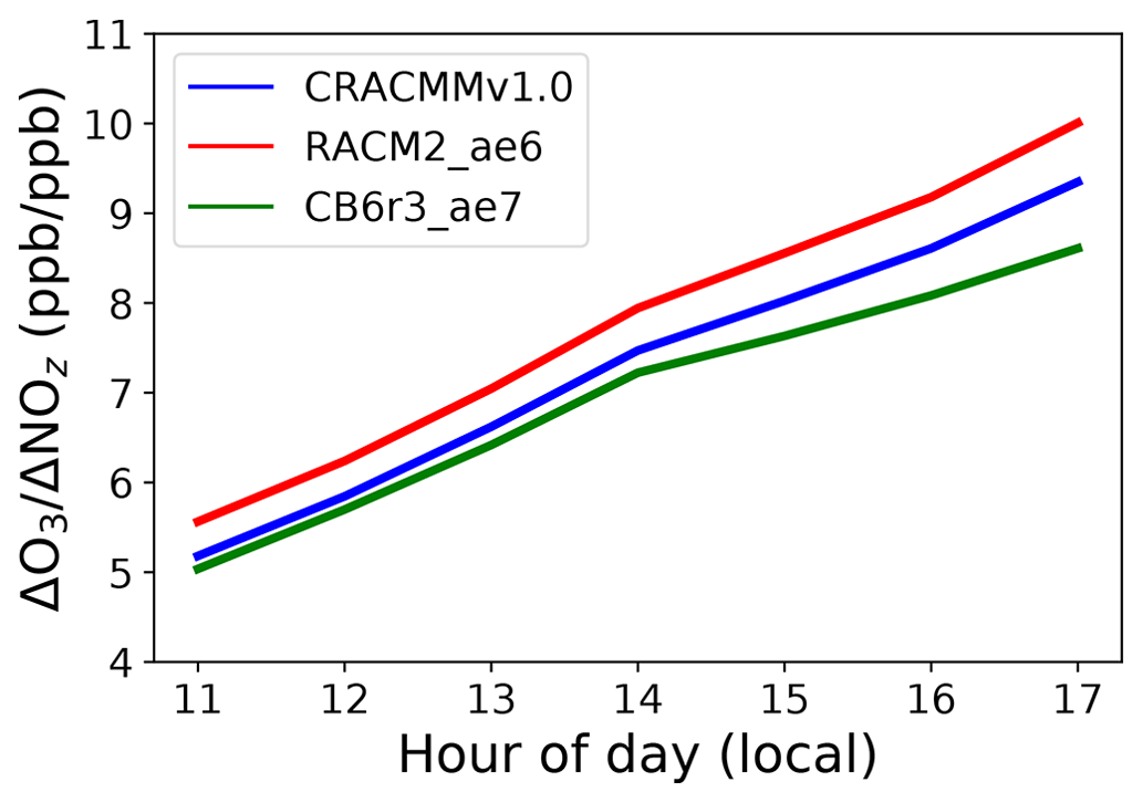
Figure 5Average domain-wide hourly ozone production efficiency (OPE) calculated from the slope of the linear regression between NOz and O3 at a given hour between 11:00 and 17:00 local time for the CRACMMv1.0, RACM2_ae6, and CB6r3_ae7 mechanism base simulations.
Figure 5 indicates that there are either differences in O3 production or NOx recycling or a combination of both between mechanisms and that these differences persist at all hours during the day. The trend in OPE values (CB6r3_ae7 < CRACMMv1.0 < RACM2_ae6) is consistent with the diurnal trends in the modeled O3 concentrations observed in Fig. 3. This trend in mechanisms was noted in a previous study model where RACM2_ae6 OPE predictions were shown to be consistently higher than Carbon Bond version 5 (specifically CB05TUCL) OPE predictions, leading to a poorer match with observations than Carbon Bond in the southeastern US (Sarwar et al., 2013). Figure 5 confirms that updates between RACM2_ae6 and CRACMMv1.0 led to decreases in OPE and improvement in CRACMM O3 predictions with observations in the northeastern US (Fig. 2; Table 1). In the following section, differences in the representation of chemical systems between RACM2_ae6 and CRACMMv1.0 that may have led to differences in ozone production and/or NOx loss between the two mechanisms are further explored.
4.3 Box model simulations
The F0AM box model (Wolfe et al., 2016) was used to further probe the mechanistic drivers of differences between the CRACMMv1.0 and RACM2 chemical mechanisms that could be important for photochemical O3 production. Note that, for this study, only the gas-phase aspects of the RACM2 base mechanism from CMAQ were ported and tested in F0AM; thus, RACM2 rather than RACM2_ae6 nomenclature will be used to refer to these results throughout this section. The box model investigation focused on RACM2 and CRACMMv1.0 because the definitions of chemical species and ROC families are similar between mechanisms, allowing for a more direct chemical comparison between the mechanisms. In addition, CRACMMv1.0 was built upon the RACM2 framework and can be more incrementally tested. Differences in chemistry between Carbon Bond- and RACM-based mechanisms have been explored previously (Sarwar et al., 2013), and detailed analyses are beyond the scope of this study.
Box model simulations were initiated in batch mode with 10 ppb of a precursor ROC, 200 ppb of H2O2 (OH source), and either 5 ppb of NO2 (NOx conditions typically observed at the Queens, NY, and Flax pond, NY, sites from Fig. 3) or 0.5 ppb NO2 (NOx conditions typically observed at the Garrett, MD, site from Fig. 3). The chemical systems were allowed to evolve for 24 h to reach steady state (see Sect. 2.5 for a full description of the model setup). The dominant fate of RO2 in simulations under high-NOx conditions was confirmed to be RO2 + NO, while simulations initiated with NOx concentrations of 0.5 ppb were dominated by RO2 + RO2 reactions. For each simulation, the evolution of O3 was monitored over time. Box model simulations were run with α-pinene, isoprene, and benzene as the ROC precursors because the α-pinene and aromatic chemical systems underwent major updates in CRACMM compared to RACM2. Additionally, the CRACMMv1.0 and RACM2 zeroed biogenic-emission and BTX emission simulations (Figs. 4 and S7–S9) showed substantial impact on ambient O3 concentration (anthropogenic-olefin chemistry, although important for O3 formation, remained unchanged between RACM2 and CRACMMv1.0).
The production of O3 over time predicted by RACM2 and CRACMMv1.0 under both high- and low-NOx conditions is plotted in Fig. 6 for all three ROC precursor system simulations. The evolution of O3 over time followed similar trends in both mechanisms and confirms that updates made to the different ROC systems in CRACMMv1.0 did not lead to massive changes in the kinetics of ozone production. For all three high-NOx (5 ppb) simulations, RACM2 led to higher-O3 predictions than CRACMMv1.0. The largest mechanism differences in O3 production occurred in the simulation run with α-pinene under higher-NOx conditions, where 31.1 ppb of O3 was produced by CRACMMv1.0 vs. 35.8 ppb produced by RACM2 by the end of the simulation (Fig. 6a). The absolute difference in O3 production between RACM2 and CRACMMv1.0 (CRACMMv1.0 − RACM2, −3.2 ppb) in the α-pinene high-NOx simulation corresponded to a relative difference of −13.1 % (Table 3). The differences in O3 between CRACCMv1.0 and RACM2 for the simulations run with isoprene (36.8 vs. 38.9 ppb of O3) and benzene (33.3 vs. 34.2 ppb of O3) under high-NOx conditions were lower than those predicted for α-pinene (Fig. 6b, c) but still indicated mechanism differences of up to −5.7 % (Table 3). The total amount of O3 produced in the three simulations under low-NOx conditions (0.5 ppb) was lower and ranged from 4.7 to 9.9 ppb (Fig. 6), with the overall changes in ozone between mechanisms very minor for the isoprene and benzene systems (O3 changes within 2.2 %). The largest relative changes in O3 production under lower-NOx conditions (−26.3 %) between the mechanisms was again observed in the simulation initiated with α-pinene.
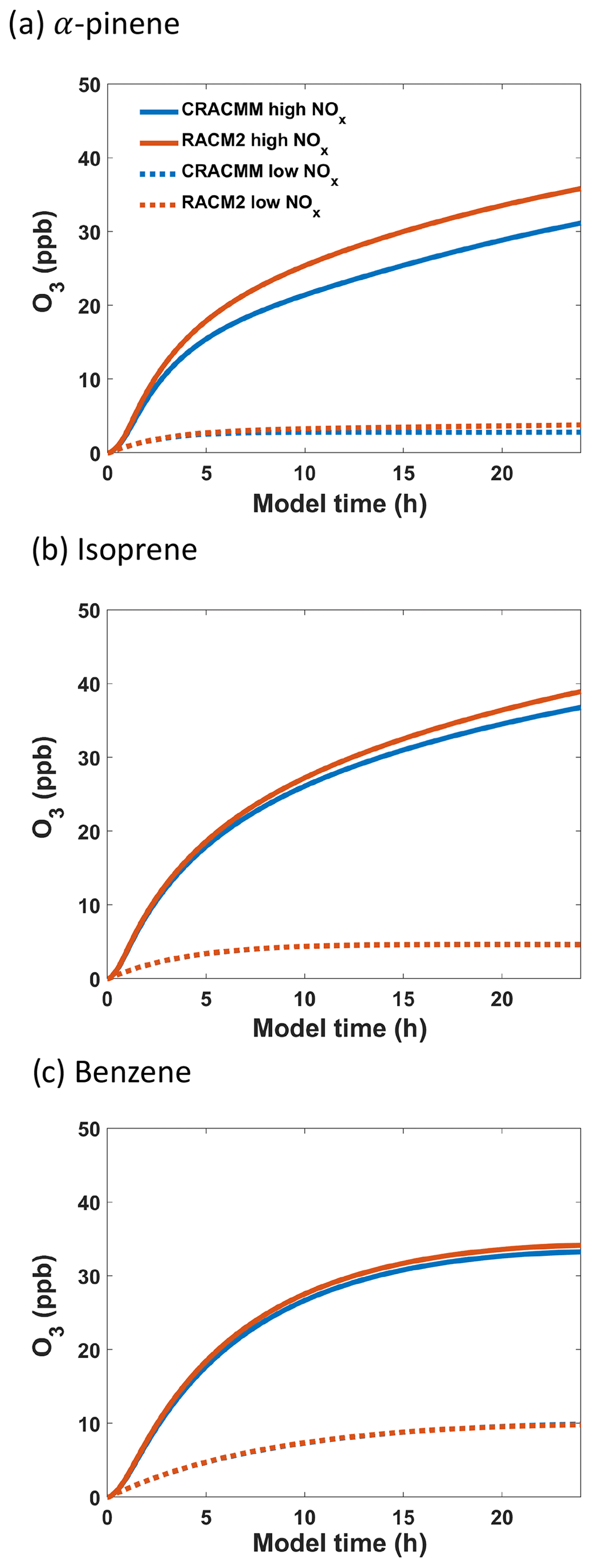
Figure 6Evolution of O3 from photochemical oxidation simulations in the F0AM box model using (a) α-pinene, (b) isoprene, and (c) benzene as ROC precursors under high-NOx (5 ppb) and low-NOx (0.5 ppb) conditions.
The absolute and relative differences in O3 production between the two mechanisms were reduced in almost all simulations when RACM2 inorganic rates were updated (RACM2_mod) to match those in CRACMMv1.0 (Table 3). The relative difference in O3 production in the simulations initiated with 5 ppb NO2 and 10 ppb ROC using RACM2_mod decreased from −13.1 % to −10.4 % in the α-pinene simulation, decreased from −5.7 % to −2.1 % in the isoprene simulation, and decreased from −2.6 % to −1.8 % in the benzene simulation. Further, in the low-NOx simulations run with RACM2_mod, O3 differences were reduced to within 0.5 % of CRACMMv1.0 for the isoprene and benzene systems. The only simulation that showed an increase in O3 production when RACM2_mod was run in place of RACM2 was the simulation run with α-pinene under low-NOx conditions, where relative differences in O3 production increased from −26.3 % to −28.2 %.
Table 3Absolute and relative differences between CRACMMv1.0 and RACM2 in the amount of ozone produced (ppb) in box model simulations run with α-pinene, isoprene and benzene under both low-NOx (0.5 ppb) and high-NOx (5 ppb) conditions. All results are reported relative to CRACMMv1.0.
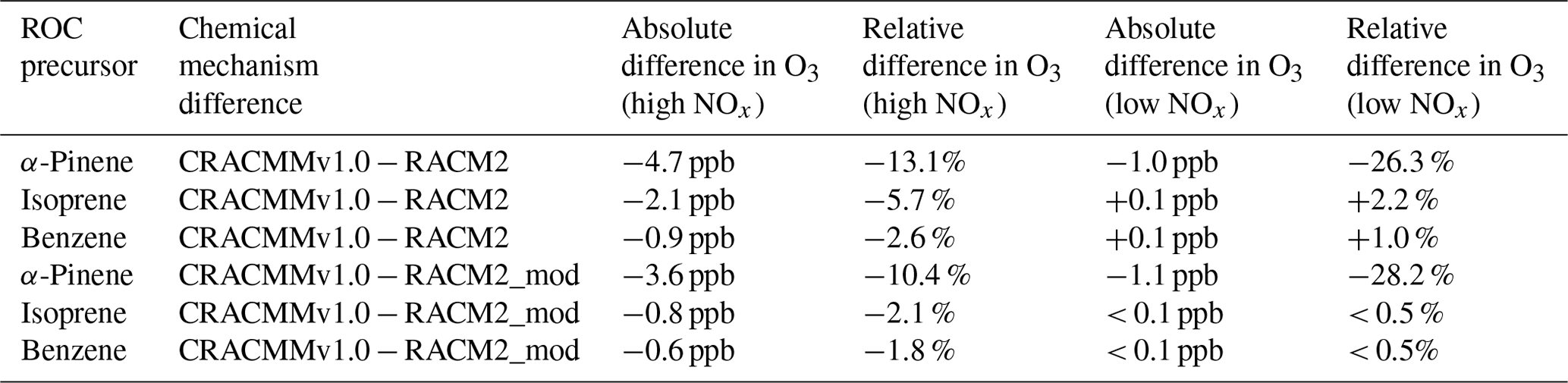
The results presented in Table 3 indicate that differences in the representation of organic chemistry in CRACMMv1.0 vs. RACM2 do partially explain the differences in O3 concentrations from CMAQ across the northeastern US model domain, given that mechanism differences in O3 production still remained in all simulations after inorganic rate constants were matched between the mechanisms. In particular, a majority of the observed O3 differences in the α-pinene–NOx–O3 system (≥ 80 %) under both high- and low-NOx conditions resulted from changes to the organic reactions alone. A large fraction of the O3 differences (∼ 70 %) in the benzene–NOx–O3 system were also driven by organic reaction updates for the simulations run with higher NOx. As anticipated, organic reaction change updates played a smaller role in the simulations with isoprene; however a difference in O3 production of 2 % still remained after running the simulations with RACM2_mod. Since RACM2_ae6 O3 predictions in CMAQ were shown to be generally biased high for the northeastern US (Table 1) and biogenic emissions were shown to be important for ozone formation (Fig. 4a), reductions in O3 production in CRACMMv1.0 contributed to the more accurate average O3 predictions across the northeastern US compared to RACM2_ae6. Previous work has found properly representing monoterpene chemistry, in particular, is important for accurately predicting organic nitrates and thereby ozone across North America (Browne et al., 2014; Fisher et al., 2016; Zare et al., 2018), including in the northeastern US (Schwantes et al., 2020).
Further investigation into the mechanisms revealed that there were also differences in the predicted loss of NOx between RACM2_mod and CRACMMv1.0 (Fig. S13) and that the differences in the evolution of NOx with time were highest in the experiment run with α-pinene. Thus, the parameterization of monoterpene reactions (which included the addition of autoxidation and explicit second-generation chemistry of monoterpene nitrates and aldehydes) led to both decreased O3 production and increased loss of NOx in CRACMMv1.0 vs. RACM2. Despite a reduction in organic nitrate yield in the benzene system (0.2 % in CRACMMv1.0 and 8.2 % in RACM2_mod), there was also higher NOx loss observed in the benzene simulation run with 5 ppb NO2 (Fig. S13). Overall, the mechanism differences in NOx loss, in addition to ozone production, are consistent with predicted differences in OPE across the northeastern US in CRACMMv1.0 vs. RACM2 (Fig. 5).
This study provides the first evaluation of O3 predictions using the newly developed CRACMMv1.0 chemical mechanism in the context of other currently available mechanisms and demonstrates CRACMMv1.0 can provide accurate ozone predictions. Average O3 predictions across CRACMMv1.0, CB6r3_ae7, and RACM2_ae6 simulations during the summer of 2018 over the northeastern US were generally within ±10 % of each other, and all had domain-wide mean biases of less than 5 ppb. Mechanism differences were most pronounced over bodies of water, where meteorology amplified differences. Over land, domain-wide O3 estimates in CRACMMv1.0 were found to be of similar magnitude to the CMAQv5.3.3.3 operational mechanism (CB6r3_ae7) (±1 ppb) but were universally lower in the mechanism upon which CRACMMv1.0 was built (RACM2_ae6) by 1–3 ppb. The lower O3 concentrations and OPE in the CRACMMv1.0 simulation compared to RACM2_ae6 resulted in better predictions of all-hour and MDA8 O3 concentrations across the NE US region as indicated by reductions in the mean bias, normalized mean bias, and normalized mean error.
CRACMMv1.0 evaluation against AQS ozone observations indicated it is more skilled at predicting ozone in locations with elevated ozone, which is important for understanding sources of exposure at concentrations most likely to cause harm. CRACMMv1.0 showed improved performance over the current CMAQ operational mechanism (CB6r3_ae7) when hourly ozone was elevated above 50 ppb. Spatially, CRACMMv1.0 showed lower bias in the northeastern US urban corridor and higher bias at rural sites, particularly in the Appalachian Mountains. Similar results were found for diurnal predictions at individual sites where CRACMM best matched O3 observations at a site that experienced higher NOx concentrations. As regional boundary conditions for CRACMMv1.0 were obtained from CB6r3_ae7, the full effects of CRACMMv1.0 on regional background air quality and long-range transport predictions have yet to be fully examined. Further, since the coupling of meteorology and chemistry has been shown to play a major role in O3 distributions, the robustness of the mechanism should also be tested on a variety of domains that encompass different terrains.
Improvements in CRACMMv1.0 compared to RACM2_ae6 O3 predictions were driven by updates to the inorganic reaction rate constants as well as updates in the representation of organic chemistry. These updates also caused slight changes in the sensitivity of ozone–ROC precursor emissions. Box model simulations in F0AM showed lower O3 production and higher NOx loss for monoterpene oxidation consistent with the lower overall OPE predicted across the northeastern US with CRACMMv1.0 compared to RACM2_ae6. The zeroed emission simulations revealed that domain-wide average O3 estimates slightly increased when emissions of S/IVOCs were omitted, suggesting the inclusion of these emissions played a role in O3 formation and mainly acted to reduce ozone. As S/IVOCs are not integrated with radical chemistry leading to ozone in RACM2_ae6 or CB6r3_ae7, some changes in the sensitivity of ozone to emissions are expected in CRACMMv1.0 compared to current mechanisms. As a further example, zeroed BTX emissions indicated rural ozone is relatively insensitive to aromatic emissions in CRACMMv1.0, whereas RACM2_ae6 (and CB6r3_ae6) predicted ozone disbenefits (increases) in the rural northeastern US when aromatic emissions were removed.
Isoprene and monoterpenes, largely from biogenic sources, are examples of chemical systems where accurate representation of their chemistry across phases is critical to improve prediction of both ozone and fine-particle endpoints. As with RACM2_ae6, CRACMMv1.0 O3 concentrations showed great sensitivity to biogenic emissions, emphasizing the need to represent their NOx cycling and radical chemistry well. In addition, autoxidation products with low volatility that sequester radicals are abundant from monoterpenes and critical for SOA formation (Pye et al., 2019). Separate work building on CRACMMv1.0 demonstrated that updated isoprene chemistry led to improved ozone predictions at high (> 50 ppb) concentrations as well as predictions of isoprene epoxydiol SOA precursors (Wiser et al., 2022). This need to have gas-phase mechanisms predict intermediates leading to SOA and have SOA products removed from the gas phase was a major motivation behind the development of CRACMM. Future evaluation of the fine-particle predictions of CRACMMv1.0 will provide even further constraints on the radical chemistry leading to ozone explored here.
The implementation of RACM2_ae6 and CB6r3_ae7 used here is available in CMAQv5.3.3 (https://doi.org/10.5281/zenodo.5213949, U.S. Environmental Protection Agency Office of Research and Development, 2021). CRACMMv1.0 is available in CMAQv5.4 (https://doi.org/10.5281/zenodo.7218076, U.S. EPA Office of Research and Development, 2022). Supporting data for CRACMM including guidance on emission preparation and species metadata (including SMILES identifiers; simplified molecular-input line-entry system) are available at https://github.com/USEPA/CRACMM (U.S. Environmental Protection Agency, 2022c and in the work of Pye et al., 2023). AMET is available at https://github.com/USEPA/AMET (U.S. Environmental Protection Agency, 2022d) and https://doi.org/10.5281/zenodo.8156171 (Appel and Gilliam, 2023). F0AM is available at https://github.com/AirChem/F0AM (Wolfe, 2022). Specific analyses and scripts used in this paper, such as the modeled and observed ozone concentrations, F0AM box model inputs, and exact CMAQ code used, are archived at https://doi.org/10.23719/1528552 (Pye, 2023).
The supplement related to this article is available online at: https://doi.org/10.5194/acp-23-9173-2023-supplement.
BKP: conceptualization, data curation, formal analysis, investigation, methodology, software, visualization, and writing – original draft preparation. WTH: resources and software (CMAQ and F0AM model code). KWA: data curation, resources, and software (observational data and processing routines). SF, BNM, KMS, GS, IRP, ELD, ES, RHS, MMC, LX, and WRS: software (CMAQ model science algorithms). LV and HS: methodology. CA, AT-V, and JP: resources (CMAQ model inputs). HOTP: conceptualization, data curation, funding acquisition, investigation, methodology, project administration, resources, software, supervision, and writing – original draft preparation. All authors reviewed and/or edited the manuscript.
The contact author has declared that none of the authors has any competing interests.
The views expressed in this article are those of the authors and do not
necessarily represent the views or policies of the U.S. Environmental
Protection Agency, Department of Energy (DOE), or Oak Ridge Institute of
Science and Education (ORISE).
Publisher’s note: Copernicus Publications remains neutral with regard to jurisdictional claims in published maps and institutional affiliations.
This work was supported by the U.S. Environmental Protection Agency Office of Research and Development. This research was supported in part by an appointment to the U.S. Environmental Protection Agency (EPA) Research Participation Program administered by ORISE through an interagency agreement between the U.S. DOE and the U.S. Environmental Protection Agency. ORISE is managed by Oak Ridge Associated Universities (ORAU; DOE contract no. DE-SC0014664). We thank Kathleen Fahey and Barron Henderson for providing comments on a draft of this paper. Matthew M. Coggon, Rebecca H. Schwantes, and Lu Xu acknowledge support through the EPA STAR program (Science to Achieve Results; grant no. 84001001) and the CIRES cooperative agreement (Cooperative Institute for Research in Environmental Science. Lu Xu also acknowledges NASA. The EPA does not endorse any products or commercial services mentioned in this publication.
This research has been supported by the U.S. Environmental Protection Agency (grant no. 84001001), the National Oceanic and Atmospheric Administration (grant no. NA17OAR4320101), and the National Aeronautics and Space Administration (grant no. 80NSSC21K1704).
This paper was edited by Joshua Fu and reviewed by two anonymous referees.
Aneja, V. P., Businger, S., Li, Z., Claiborn, C. S., and Murthy, A.: Ozone Climatology at High Elevations in the Southern Appalachians, J. Geophys. Res.-Atmos., 96, 1007–1021, https://doi.org/10.1029/90jd02022, 1991.
Appel, K. W. and Gilliam, R.: USEPA/AMET: AMETv1.5, Zenodo [code], https://doi.org/10.5281/zenodo.8156171 (last access: 9 August 2023), 2023.
Appel, K. W., Gilliam, R. C., Davis, N., Zubrow, A., and Howard, S. C.: Overview of the atmospheric model evaluation tool (AMET) v1.1 for evaluating meteorological and air quality models, Environ. Modell. Softw., 26, 434–443, https://doi.org/10.1016/j.envsoft.2010.09.007, 2011.
Appel, K. W., Bash, J. O., Fahey, K. M., Foley, K. M., Gilliam, R. C., Hogrefe, C., Hutzell, W. T., Kang, D., Mathur, R., Murphy, B. N., Napelenok, S. L., Nolte, C. G., Pleim, J. E., Pouliot, G. A., Pye, H. O. T., Ran, L., Roselle, S. J., Sarwar, G., Schwede, D. B., Sidi, F. I., Spero, T. L., and Wong, D. C.: The Community Multiscale Air Quality (CMAQ) model versions 5.3 and 5.3.1: system updates and evaluation, Geosci. Model Dev., 14, 2867–2897, https://doi.org/10.5194/gmd-14-2867-2021, 2021.
Arnold, J. R., Dennis, R. L., and Tonnesen, G. S.: Diagnostic evaluation of numerical air quality models with specialized ambient observations: testing the Community Multiscale Air Quality modeling system (CMAQ) at selected SOS 95 ground sites, Atmos. Environ., 37, 1185–1198, https://doi.org/10.1016/S1352-2310(02)01008-7, 2003.
Bachmann, J.: Will the Circle Be Unbroken: A History of the U.S. National Ambient Air Quality Standards, J. Air Waste Manage., 57, 652–697, https://doi.org/10.3155/1047-3289.57.6.652, 2007.
Bash, J. O., Baker, K. R., and Beaver, M. R.: Evaluation of improved land use and canopy representation in BEIS v3.61 with biogenic VOC measurements in California, Geosci. Model Dev., 9, 2191–2207, https://doi.org/10.5194/gmd-9-2191-2016, 2016.
Bell, M. L., Dominici, F., and Samet, J. M.: A meta-analysis of time-series studies of ozone and mortality with comparison to the national morbidity, mortality, and air pollution study, Epidemiology, 16, 436–445, https://doi.org/10.1097/01.ede.0000165817.40152.85, 2005.
Brasseur, G. P., Kiehl, J. T., Muller, J. F., Schneider, T., Granier, C., Tie, X. X., and Hauglustaine, D.: Past and future changes in global tropospheric ozone: Impact on radiative forcing, Geophys. Res. Lett., 25, 3807–3810, https://doi.org/10.1029/1998gl900013, 1998.
Browne, E. C., Wooldridge, P. J., Min, K.-E., and Cohen, R. C.: On the role of monoterpene chemistry in the remote continental boundary layer, Atmos. Chem. Phys., 14, 1225–1238, https://doi.org/10.5194/acp-14-1225-2014, 2014.
Carter, W. P. L.: A Detailed Mechanism for the Gas-Phase Atmospheric Reactions of Organic-Compounds, Atmos. Environ. A-Gen., 24, 481–518, https://doi.org/10.1016/0960-1686(90)90005-8, 1990.
Cheng, P. Y., Pour-Biazar, A., White, A. T., and McNider, R. T.: Improvement of summertime surface ozone prediction by assimilating Geostationary Operational Environmental Satellite cloud observations, Atmos. Environ., 268, 118751, https://doi.org/10.1016/j.atmosenv.2021.118751, 2022.
Cleary, P. A., Dickens, A., McIlquham, M., Sanchez, M., Geib, K., Hedberg, C., Hupy, J., Watson, M. W., Fuoco, M., Olson, E. R., Pierce, R. B., Stanier, C., Long, R., Valin, L., Conley, S., and Smith, M.: Impacts of lake breeze meteorology on ozone gradient observations along Lake Michigan shorelines in Wisconsin, Atmos. Environ., 269, 118834, https://doi.org/10.1016/j.atmosenv.2021.118834, 2022.
Dodge, M. C.: Chemical oxidant mechanisms for air quality modeling: critical review, Atmos. Environ., 34, 2103–2130, https://doi.org/10.1016/S1352-2310(99)00461-6, 2000.
Dreessen, J., Orozco, D., Boyle, J., Szymborski, J., Lee, P., Flores, A., and Sakai, R. K.: Observed ozone over the Chesapeake Bay land-water interface: The Hart-Miller Island Pilot Project, J. Air Waste Manage., 69, 1312–1330, https://doi.org/10.1080/10962247.2019.1668497, 2019.
Dye, T. S., Roberts, P. T., and Korc, M. E.: Observations of Transport Processes for Ozone and Ozone Precursors during the 1991 Lake-Michigan Ozone Study, J. Appl. Meteorol., 34, 1877–1889, https://doi.org/10.1175/1520-0450(1995)034<1877:Ootpfo>2.0.Co;2, 1995.
Emery, C., Liu, Z., Russell, A. G., Odman, M. T., Yarwood, G., and Kumar, N.: Recommendations on statistics and benchmarks to assess photochemical model performance, J. Air Waste Manage., 67, 582–598, https://doi.org/10.1080/10962247.2016.1265027, 2017.
Fisher, J. A., Jacob, D. J., Travis, K. R., Kim, P. S., Marais, E. A., Chan Miller, C., Yu, K., Zhu, L., Yantosca, R. M., Sulprizio, M. P., Mao, J., Wennberg, P. O., Crounse, J. D., Teng, A. P., Nguyen, T. B., St. Clair, J. M., Cohen, R. C., Romer, P., Nault, B. A., Wooldridge, P. J., Jimenez, J. L., Campuzano-Jost, P., Day, D. A., Hu, W., Shepson, P. B., Xiong, F., Blake, D. R., Goldstein, A. H., Misztal, P. K., Hanisco, T. F., Wolfe, G. M., Ryerson, T. B., Wisthaler, A., and Mikoviny, T.: Organic nitrate chemistry and its implications for nitrogen budgets in an isoprene- and monoterpene-rich atmosphere: constraints from aircraft (SEAC4RS) and ground-based (SOAS) observations in the Southeast US, Atmos. Chem. Phys., 16, 5969–5991, https://doi.org/10.5194/acp-16-5969-2016, 2016.
Fiore, A. M., Horowitz, L. W., Purves, D. W., Levy II, H., Evans, M. J., Wang, Y., Li, Q., and Yantosca, R. M.: Evaluating the contribution of changes in isoprene emissions to surface ozone trends over the eastern United States, J. Geophys. Res.-Atmos., 110, 2004JD005485, https://doi.org/10.1029/2004JD005485, 2005.
Foley, T., Betterton, E. A., Robert Jacko, P. E., and Hillery, J.: Lake Michigan air quality: The 1994–2003 LADCO Aircraft Project (LAP), Atmos. Environ., 45, 3192–3202, https://doi.org/10.1016/j.atmosenv.2011.02.033, 2011.
Gery, M. W., Whitten, G. Z., Killus, J. P., and Dodge, M. C.: A Photochemical Kinetics Mechanism for Urban and Regional Scale Computer Modeling, J. Geophys. Res.-Atmos., 94, 12925–12956, https://doi.org/10.1029/JD094iD10p12925, 1989.
Ghosh, A., Singh, A. A., Agrawal, M., and Agrawal, S. B.: Ozone Toxicity and Remediation in Crop Plants, Sustain. Agr. Rev., 27, 129–169, https://doi.org/10.1007/978-3-319-75190-0_5, 2018.
Goliff, W. S., Stockwell, W. R., and Lawson, C. V.: The regional atmospheric chemistry mechanism, version 2, Atmos. Environ., 68, 174–185, https://doi.org/10.1016/j.atmosenv.2012.11.038, 2013.
Heald, C. L. and Kroll, J. H.: The fuel of atmospheric chemistry: Toward a complete description of reactive organic carbon, Sci. Adv., 6, eaay8967, https://doi.org/10.1126/sciadv.aay8967, 2020.
Henneman, L. R. F., Shen, H., Liu, C., Hu, Y., Mulholland, J. A., and Russell, A. G.: Responses in Ozone and Its Production Efficiency Attributable to Recent and Future Emissions Changes in the Eastern United States, Environ. Sci. Technol., 51, 13797–13805, https://doi.org/10.1021/acs.est.7b04109, 2017.
Hogrefe, C., Lynn, B., Civerolo, K., Ku, J.-Y., Rosenthal, J., Rosenzweig, C., Goldberg, R., Gaffin, S., Knowlton, K., and Kinney, P. L.: Simulating changes in regional air pollution over the eastern United States due to changes in global and regional climate and emissions, J. Geophys. Res.-Atmos., 109, 2004JD004690, https://doi.org/10.1029/2004JD004690, 2004.
Iriti, M. and Faoro, F.: Oxidative stress, the paradigm of ozone toxicity in plants and animals, Water Air Soil Poll., 187, 285–301, https://doi.org/10.1007/s11270-007-9517-7, 2008.
Jacob, D. J.: Introduction to Atmospheric Chemistry, Princeton University Press, ISBN 9780691001852, 1999.
Jenkin, M. E., Young, J. C., and Rickard, A. R.: The MCM v3.3.1 degradation scheme for isoprene, Atmos. Chem. Phys., 15, 11433–11459, https://doi.org/10.5194/acp-15-11433-2015, 2015.
Koo, B., Knipping, E., and Yarwood, G.: 1.5-Dimensional volatility basis set approach for modeling organic aerosol in CAMx and CMAQ, Atmos. Environ., 95, 158–164, https://doi.org/10.1016/j.atmosenv.2014.06.031, 2014.
Larrieu, S., Jusot, J. F., Blanchard, M., Prouvost, H., Declercq, C., Fabre, P., Pascal, L., Le Tertre, A., Wagner, V., Riviere, S., Chardon, B., Borrelli, D., Cassadou, S., Eilstein, D., and Lefranc, A.: Short term effects of air pollution on hospitalizations for cardiovascular diseases in eight French cities: The PSAS program, Sci. Total Environ., 387, 105–112, https://doi.org/10.1016/j.scitotenv.2007.07.025, 2007.
Lennartson, G. J. and Schwartz, M. D.: The lake breeze-ground-level ozone connection in eastern Wisconsin: A climatological perspective, Int. J. Climatol., 22, 1347–1364, https://doi.org/10.1002/joc.802, 2002.
Li, X. S. and Rappenglueck, B.: A study of model nighttime ozone bias in air quality modeling, Atmos. Environ., 195, 210–228, https://doi.org/10.1016/j.atmosenv.2018.09.046, 2018.
Lu, Q., Murphy, B. N., Qin, M., Adams, P. J., Zhao, Y., Pye, H. O. T., Efstathiou, C., Allen, C., and Robinson, A. L.: Simulation of organic aerosol formation during the CalNex study: updated mobile emissions and secondary organic aerosol parameterization for intermediate-volatility organic compounds, Atmos. Chem. Phys., 20, 4313–4332, https://doi.org/10.5194/acp-20-4313-2020, 2020.
Mathur, R., Xing, J., Gilliam, R., Sarwar, G., Hogrefe, C., Pleim, J., Pouliot, G., Roselle, S., Spero, T. L., Wong, D. C., and Young, J.: Extending the Community Multiscale Air Quality (CMAQ) modeling system to hemispheric scales: overview of process considerations and initial applications, Atmos. Chem. Phys., 17, 12449–12474, https://doi.org/10.5194/acp-17-12449-2017, 2017.
Mohr, C., Huffman, J. A., Cubison, M. J., Aiken, A. C., Docherty, K. S., Kimmel, J. R., Ulbrich, I. M., Hannigan, M., and Jimenez, J. L.: Characterization of Primary Organic Aerosol Emissions from Meat Cooking, Trash Burning, and Motor Vehicles with High-Resolution Aerosol Mass Spectrometry and Comparison with Ambient and Chamber Observations, Environ. Sci. Technol., 43, 2443–2449, https://doi.org/10.1021/es8011518, 2009.
Murphy, B. N., Woody, M. C., Jimenez, J. L., Carlton, A. M. G., Hayes, P. L., Liu, S., Ng, N. L., Russell, L. M., Setyan, A., Xu, L., Young, J., Zaveri, R. A., Zhang, Q., and Pye, H. O. T.: Semivolatile POA and parameterized total combustion SOA in CMAQv5.2: impacts on source strength and partitioning, Atmos. Chem. Phys., 17, 11107–11133, https://doi.org/10.5194/acp-17-11107-2017, 2017.
Murphy, B. N., Nolte, C. G., Sidi, F., Bash, J. O., Appel, K. W., Jang, C., Kang, D., Kelly, J., Mathur, R., Napelenok, S., Pouliot, G., and Pye, H. O. T.: The Detailed Emissions Scaling, Isolation, and Diagnostic (DESID) module in the Community Multiscale Air Quality (CMAQ) modeling system version 5.3.2, Geosci. Model Dev., 14, 3407–3420, https://doi.org/10.5194/gmd-14-3407-2021, 2021.
Neufeld, H. S., Sullins, A., Sive, B. C., and Lefohn, A. S.: Spatial and temporal patterns of ozone at Great Smoky Mountains National Park and implications for plant responses, Atmos. Environ., 2, 100023, https://doi.org/10.1016/j.aeaoa.2019.100023, 2019.
Otte, T. L. and Pleim, J. E.: The Meteorology-Chemistry Interface Processor (MCIP) for the CMAQ modeling system: updates through MCIPv3.4.1, Geosci. Model Dev., 3, 243–256, https://doi.org/10.5194/gmd-3-243-2010, 2010.
Pye, H.: Data for Sensitivity of Northeast U.S. surface ozone predictions to the representation of atmospheric chemistry in CRACMMv1.0, U.S. EPA Office of Research and Development [data set and code], https://doi.org/10.23719/1528552 (last access: 7 May 2023), 2023.
Pye, H. O. T., Chan, A. W. H., Barkley, M. P., and Seinfeld, J. H.: Global modeling of organic aerosol: the importance of reactive nitrogen (NOx and NO3), Atmos. Chem. Phys., 10, 11261–11276, https://doi.org/10.5194/acp-10-11261-2010, 2010.
Pye, H. O. T., Luecken, D. J., Xu, L., Boyd, C. M., Ng, N. L., Baker, K. R., Ayres, B. R., Bash, J. O., Baumann, K., Carter, W. P. L., Edgerton, E., Fry, J. L., Hutzell, W. T., Schwede, D. B., and Shepson, P. B.: Modeling the current and future roles of particulate organic nitrates in the southeastern United States, Environ. Sci. Technol., 49, 14195–14203, https://doi.org/10.1021/acs.est.5b03738, 2015.
Pye, H. O. T., D'Ambro, E. L., Lee, B. H., Schobesberger, S., Takeuchi, M., Zhao, Y., Lopez-Hilfiker, F., Liu, J., Shilling, J. E., Xing, J., Mathur, R., Middlebrook, A. M., Liao, J., Welti, A., Graus, M., Warneke, C., de Gouw, J. A., Holloway, J. S., Ryerson, T. B., Pollack, I. B., and Thornton, J. A.: Anthropogenic enhancements to production of highly oxygenated molecules from autoxidation, P. Natl. Acad. Sci. USA, 116, 6641, https://doi.org/10.1073/pnas.1810774116, 2019.
Pye, H. O. T., Place, B. K., Murphy, B. N., Seltzer, K. M., D'Ambro, E. L., Allen, C., Piletic, I. R., Farrell, S., Schwantes, R. H., Coggon, M. M., Saunders, E., Xu, L., Sarwar, G., Hutzell, W. T., Foley, K. M., Pouliot, G., Bash, J., and Stockwell, W. R.: Linking gas, particulate, and toxic endpoints to air emissions in the Community Regional Atmospheric Chemistry Multiphase Mechanism (CRACMM), Atmos. Chem. Phys., 23, 5043–5099, https://doi.org/10.5194/acp-23-5043-2023, 2023.
Rich, D. Q., Mittleman, M. A., Link, M. S., Schwartz, J., Luttmann-Gibson, H., Catalano, P. J., Speizer, F. E., Gold, D. R., and Dockery, D. W.: Increased risk of paroxysmal atrial fibrillation episodes associated with acute increases in ambient air pollution, Environ. Health Persp., 114, 120–123, https://doi.org/10.1289/ehp.8371, 2006.
Sarwar, G., Luecken, D., Yarwood, G., Whitten, G. Z., and Carter, W. P. L.: Impact of an updated carbon bond mechanism on predictions from the CMAQ modeling system: Preliminary assessment, J. Appl. Meteorol., 47, 3–14, https://doi.org/10.1175/2007jamc1393.1, 2008.
Sarwar, G., Godowitch, J., Henderson, B. H., Fahey, K., Pouliot, G., Hutzell, W. T., Mathur, R., Kang, D., Goliff, W. S., and Stockwell, W. R.: A comparison of atmospheric composition using the Carbon Bond and Regional Atmospheric Chemistry Mechanisms, Atmos. Chem. Phys., 13, 9695–9712, https://doi.org/10.5194/acp-13-9695-2013, 2013.
Schwantes, R. H., Emmons, L. K., Orlando, J. J., Barth, M. C., Tyndall, G. S., Hall, S. R., Ullmann, K., St. Clair, J. M., Blake, D. R., Wisthaler, A., and Bui, T. P. V.: Comprehensive isoprene and terpene gas-phase chemistry improves simulated surface ozone in the southeastern US, Atmos. Chem. Phys., 20, 3739–3776, https://doi.org/10.5194/acp-20-3739-2020, 2020.
Seinfeld, J. H. and Pandis, S. N.: Atmospheric Chemistry and Physics: From Air Pollution to Climate Change, John Wiley & Sonds, New York, ISBN 0471720186, 2006.
Seltzer, K. M., Pennington, E., Rao, V., Murphy, B. N., Strum, M., Isaacs, K. K., and Pye, H. O. T.: Reactive organic carbon emissions from volatile chemical products, Atmos. Chem. Phys., 21, 5079–5100, https://doi.org/10.5194/acp-21-5079-2021, 2021.
Seltzer, K. M., Murphy, B. N., Pennington, E. A., Allen, C., Talgo, K., and Pye, H. O. T.: Volatile Chemical Product Enhancements to Criteria Pollutants in the United States, Environ. Sci. Technol., 56, 6905–6913, https://doi.org/10.1021/acs.est.1c04298, 2022.
Sillman, S., Samson, P. J., and Masters, J. M.: Ozone Production in Urban Plumes Transported over Water – Photochemical Model and Case-Studies in the Northeastern and Midwestern United-States, J. Geophys. Res.-Atmos., 98, 12687–12699, https://doi.org/10.1029/93jd00159, 1993.
Simon, H., Baker, K. R., and Phillips, S.: Compilation and interpretation of photochemical model performance statistics published between 2006 and 2012, Atmos. Environ., 61, 124–139, https://doi.org/10.1016/j.atmosenv.2012.07.012, 2012.
Solazzo, E., Hogrefe, C., Colette, A., Garcia-Vivanco, M., and Galmarini, S.: Advanced error diagnostics of the CMAQ and Chimere modelling systems within the AQMEII3 model evaluation framework, Atmos. Chem. Phys., 17, 10435–10465, https://doi.org/10.5194/acp-17-10435-2017, 2017.
Stevenson, D. S., Young, P. J., Naik, V., Lamarque, J.-F., Shindell, D. T., Voulgarakis, A., Skeie, R. B., Dalsoren, S. B., Myhre, G., Berntsen, T. K., Folberth, G. A., Rumbold, S. T., Collins, W. J., MacKenzie, I. A., Doherty, R. M., Zeng, G., van Noije, T. P. C., Strunk, A., Bergmann, D., Cameron-Smith, P., Plummer, D. A., Strode, S. A., Horowitz, L., Lee, Y. H., Szopa, S., Sudo, K., Nagashima, T., Josse, B., Cionni, I., Righi, M., Eyring, V., Conley, A., Bowman, K. W., Wild, O., and Archibald, A.: Tropospheric ozone changes, radiative forcing and attribution to emissions in the Atmospheric Chemistry and Climate Model Intercomparison Project (ACCMIP), Atmos. Chem. Phys., 13, 3063–3085, https://doi.org/10.5194/acp-13-3063-2013, 2013.
Stockwell, W. R., Kirchner, F., Kuhn, M., and Seefeld, S.: A new mechanism for regional atmospheric chemistry modeling, J. Geophys. Res.-Atmos., 102, 25847–25879, https://doi.org/10.1029/97JD00849, 1997.
Stockwell, W. R., Lawson, C. V., Saunders, E., and Goliff, W. S.: A Review of Tropospheric Atmospheric Chemistry and Gas-Phase Chemical Mechanisms for Air Quality Modeling, Atmosphere-Basel, 3, 1–32, https://doi.org/10.3390/atmos3010001, 2012.
Torres-Vazquez, A., Pleim, J., Gilliam, R., and Pouliot, G.: Performance Evaluation of the Meteorology and Air Quality Conditions from Multiscale WRF-CMAQ Simulations for the Long Island Sound Tropospheric Ozone Study (LISTOS), J. Geophys. Res.-Atmos., 127, e2021JD035890, https://doi.org/10.1029/2021JD035890, 2022.
U.S. Environmental Protection Agency: National Ambient Air Quality Standards for Ozone, Washington, D.C.EPA-HQ-OAR-2008-0699, https://www.federalregister.gov/documents/2015/10/26/2015-26594/national-ambient-air-quality-standards-for-ozone (last access: 9 August 2023), 2015.
U.S. Environmental Protection Agency: Technical support document (TSD) preparation of emissions inventories for the version 7.2 2016 North American emissions modeling platform, Research Triangle Park, NC, https://www.epa.gov/air-emissions-modeling/2016-version-72-technical-support-document (last access: 9 August 2023), 2019.
U.S. Environmental Protection Agency: Integrated science assessment for ozone and related photochemical oxidants U.S. Environmental Protection Agency, Washington, D.C.EPA/600/R-20/012, https://www.epa.gov/isa/integrated-science-assessment-isa-ozone-and-related-photochemical-oxidants (last access: 9 August 2023), 2020.
U.S. Environmental Protection Agency: Nonattainment Areas for Criteria Pollutants (Green Book), https://www.epa.gov/green-book (last access: 13 May 2022), 2022a.
U.S. Environmental Protection Agency: CMAQ: The Community Multiscale Air Quality Modeling System, https://www.epa.gov/cmaq (last access: 21 November 2022), 2022b.
U.S. Environmental Protection Agency: CRACMM, GitHub [data set], https://github.com/USEPA/CRACMM (last access: 21 November 2022), 2022c.
U.S. Environmental Protection Agency: Atmospheric Model Evaluation Tool (AMETv1.5), GitHub [code], https://github.com/USEPA/AMET (last access: 21 November 2022), 2022d.
U.S. Environmental Protection Agency Office of Research and Development: CMAQ (Version 5.3.3), Zenodo [code], https://doi.org/10.5281/zenodo.5213949, (last access: 8 August 2023), 2021.
U.S. EPA Office of Research and Development: CMAQ Version 5.4, Zenodo [code], https://doi.org/10.5281/zenodo.7218076, 2022.
Vermeuel, M. P., Novak, G. A., Alwe, H. D., Hughes, D. D., Kaleel, R., Dickens, A. F., Kenski, D., Czarnetzki, A. C., Stone, E. A., Stanier, C. O., Pierce, R. B., Millet, D. B., and Bertram, T. H.: Sensitivity of Ozone Production to NOx and VOC Along the Lake Michigan Coastline, J. Geophys. Res.-Atmos., 124, 10989–11006, https://doi.org/10.1029/2019jd030842, 2019.
Warneke, C., Schwantes, R., Veres, P., Rollins, A., Brewer, W. A., McDonald, B., Brown, S., Frost, G., Fahey, D., Aikin, K., Judd, L., Lefer, B., Pierce, R. B., Kondragunta, S., Stockwell, C., Gentner, D., Krechmer, J., Lambe, A., Millet, D., Farmer, D., Ng, N. L., Kaiser, J., Young, C., Mak, J., Wolfe, G., Sullivan, J., Mueller, K., Karion, A., Valin, L., Witte, M., Russell, L., Ren, X., Dickerson, R., and Decarlo, P.: The AEROMMA 2023 experiment (Atmospheric Emissions and Reactions Observed from Megacities to Marine Areas), https://csl.noaa.gov/projects/aeromma/whitepaper.pdf (last access: 9 August 2023), 2022.
Wiser, F., Place, B. K., Sen, S., Pye, H. O. T., Yang, B., Westervelt, D. M., Henze, D. K., Fiore, A. M., and McNeill, V. F.: AMORE-Isoprene v1.0: a new reduced mechanism for gas-phase isoprene oxidation, Geosci. Model Dev., 16, 1801–1821, https://doi.org/10.5194/gmd-16-1801-2023, 2023.
Wolfe, G. M.: Framework for 0-D Atmospheric Modeling, GitHub [code], https://github.com/AirChem/F0AM (last access: 21 November 2022), 2022.
Wolfe, G. M., Marvin, M. R., Roberts, S. J., Travis, K. R., and Liao, J.: The Framework for 0-D Atmospheric Modeling (F0AM) v3.1, Geosci. Model Dev., 9, 3309–3319, https://doi.org/10.5194/gmd-9-3309-2016, 2016.
Woody, M. C., Baker, K. R., Hayes, P. L., Jimenez, J. L., Koo, B., and Pye, H. O. T.: Understanding sources of organic aerosol during CalNex-2010 using the CMAQ-VBS, Atmos. Chem. Phys., 16, 4081–4100, https://doi.org/10.5194/acp-16-4081-2016, 2016.
Xu, L., Pye, H. O. T., He, J., Chen, Y., Murphy, B. N., and Ng, N. L.: Experimental and model estimates of the contributions from biogenic monoterpenes and sesquiterpenes to secondary organic aerosol in the southeastern United States, Atmos. Chem. Phys., 18, 12613–12637, https://doi.org/10.5194/acp-18-12613-2018, 2018.
Xu, L., Møller, K. H., Crounse, J. D., Kjaergaard, H. G., and Wennberg, P. O.: New Insights into the Radical Chemistry and Product Distribution in the OH-Initiated Oxidation of Benzene, Environ. Sci. Technol., 54, 13467–13477, https://doi.org/10.1021/acs.est.0c04780, 2020.
Yu, S., Mathur, R., Sarwar, G., Kang, D., Tong, D., Pouliot, G., and Pleim, J.: Eta-CMAQ air quality forecasts for O3 and related species using three different photochemical mechanisms (CB4, CB05, SAPRC-99): comparisons with measurements during the 2004 ICARTT study, Atmos. Chem. Phys., 10, 3001–3025, https://doi.org/10.5194/acp-10-3001-2010, 2010.
Zare, A., Romer, P. S., Nguyen, T., Keutsch, F. N., Skog, K., and Cohen, R. C.: A comprehensive organic nitrate chemistry: insights into the lifetime of atmospheric organic nitrates, Atmos. Chem. Phys., 18, 15419–15436, https://doi.org/10.5194/acp-18-15419-2018, 2018.