the Creative Commons Attribution 4.0 License.
the Creative Commons Attribution 4.0 License.
 | 08 Aug 2023
The characteristics of atmospheric boundary layer height over the Arctic Ocean during MOSAiC
Shijie Peng
Qinghua Yang
Matthew D. Shupe
Xingya Xi
Bo Han
Dake Chen
Sandro Dahlke
The important roles that the atmospheric boundary layer (ABL) plays in the central Arctic climate system have been recognized, but the atmospheric boundary layer height (ABLH), defined as the layer of continuous turbulence adjacent to the surface, has rarely been investigated. Using a year-round radiosonde dataset during the Multidisciplinary drifting Observatory for the Study of Arctic Climate (MOSAiC) expedition, we improve a Richardson-number-based algorithm that takes cloud effects into consideration and subsequently analyze the characteristics and variability of the ABLH over the Arctic Ocean. The results reveal that the annual cycle is clearly characterized by a distinct peak in May and two respective minima in January and July. This annual variation in the ABLH is primarily controlled by the evolution of the ABL thermal structure. Temperature inversions in the winter and summer are intensified by seasonal radiative cooling and warm-air advection with the surface temperature constrained by melting, respectively, leading to the low ABLH at these times. Meteorological and turbulence variables also play a significant role in ABLH variation, including the near-surface potential temperature gradient, friction velocity, and turbulent kinetic energy (TKE) dissipation rate. In addition, the MOSAiC ABLH is more suppressed than the ABLH during the Surface Heat Budget of the Arctic Ocean (SHEBA) experiment in the summer, which indicates that there is large variability in the Arctic ABL structure during the summer melting season.
- Article
(7680 KB) - Full-text XML
- BibTeX
- EndNote


In recent years, rapid climate change and declining sea ice in the Arctic have been reported by numerous studies (e.g., Matveeva and Semenov, 2022; Meier and Stroeve, 2022; Esau et al., 2023). The Arctic near-surface temperature is increasing at a rate that is 2–3 times faster than the global average, which is referred to as Arctic amplification (Overland et al., 2019; Blunden and Arndt, 2019), and the Arctic has entered the “new Arctic” period (Landrum and Holland, 2020). As a key component of the Arctic climate system, the atmospheric boundary layer (ABL) over the Arctic Ocean is closely associated with Arctic warming and has a large impact on sea-ice loss (Francis and Hunter, 2006; Graversen et al., 2008; Wetzel and Bruemmer, 2011). Thus, it is critical to improve our understanding of Arctic ABL processes under new Arctic conditions.
The ABL structure over the Arctic Ocean has unique characteristics due to the presence of semipermanent sea ice, and it is shaped by various mechanisms, including interactions with the surface, free atmosphere, and wave activity. Most studies of the Arctic ABL structure have been based on coastal observatories and limited drifting ice stations (Knudsen et al., 2018; Vullers et al., 2021). It has been found that a predominant temperature inversion in the lower troposphere exists in all seasons, and this is referred to as the “Arctic inversion” (Andreas et al., 2000; Tjernström et al., 2009). The Arctic inversion is sometimes elevated, with regions of near-neutral stability below the inversion (Persson et al., 2002; Tjernström et al., 2012). The Arctic vertical structure is influenced by many factors, such as warm-air advection, surface melt, cloud-top cooling, and turbulent mixing (Busch et al., 1982; Vihma et al., 2011; Vihma, 2014). Investigations of the ABL structure evolution and its controlling factors are the key to establishing the ABL's role in the Arctic atmosphere (Sterk et al., 2014).
The atmospheric boundary layer height (ABLH), here defined as the height of continuous turbulent mixing extending up from the surface, is the key indicator of the ABL structure (Seibert et al., 2000; Seidel et al., 2012). It determines the vertical extent of many atmospheric processes, such as convective transport and aerosol distribution, and is an important parameter for weather and climate models (Holtslag et al., 2013; Mahrt, 2014; Davy and Esau, 2016). In some previous studies, the ABLH over the Arctic Ocean has been defined as the height of the surfaced-based inversion top or the capping inversion base (e.g., Tjernström et al., 2009; Sotiropoulou et al., 2014). However, as the most fundamental characteristic of the ABL, turbulence is not fully considered in this definition. There are two primary layers of turbulent mixing in the Arctic atmosphere. First, the surface layer, formed by turbulent mixing processes near the surface, is frequently shallower than the Arctic inversion layer (Mahrt, 1981; Andreas et al., 2000). Second, the turbulence associated with low-level clouds, which is driven by radiative cooling near the cloud top, forms a cloud-induced mixed layer (Solomon et al., 2011; Shupe et al., 2013). This cloud-driven mixed layer is sometimes decoupled from the surface mixed layer, whereas it extends down to form a coupled, well-mixed layer all the way to the surface at other times (Shupe et al., 2013; Brooks et al., 2017). Wind-shear-induced turbulence can also play a role in both of these layers and their interactions. Based on different turbulence characteristics, the ABLH is commonly determined using profiles of potential temperature, wind speed, and humidity, and various methods have been proposed for calculating the ABLH (Seibert et al., 2000; Seidel et al., 2010). However, the applicability of these methods in the Arctic needs to be further assessed.
Due to the lack of observations, there are few analyses of the ABLH over the Arctic Ocean based on observational data. Distributions of the Arctic ABLH have been investigated by Tjernström and Graversen (2009), Liu and Liang (2010), and Dai et al. (2011), but their studies were all based on the Surface Heat Budget of the Arctic Ocean (SHEBA) campaign conducted 25 years ago (Uttal et al., 2002). To improve our understanding of the ABL structure and ABLH characteristics under new Arctic conditions, we need new, comprehensive observations in this environment. The Multidisciplinary drifting Observatory for the Study of Arctic Climate (MOSAiC) expedition was, in part, designed to achieve this goal (Shupe et al., 2022). Based on and around a drifting research vessel in the central Arctic for a whole year, the MOSAiC expedition provided a wealth of data and related data products with an unprecedented high temporal resolution and year-round temporal coverage. These data make a more detailed analysis of the ABL structure evolution and ABLH variability possible.
In this study, based on observational data from the MOSAiC expedition, we propose an improved ABLH algorithm and then examine the characteristics of the ABL evolution over the new Arctic sea-ice surface. This paper is organized as follows: Sect. 2 briefly describes the MOSAiC expedition and the observations; Sect. 3 provides an ABLH determination method to evaluate several automated algorithms, and develops an improved ABLH algorithm; Sect. 4 presents the results with respect to the ABLH variation over the annual cycle, the controlling factors of ABLH variation, and mechanisms of ABL development and suppression; Sect. 5 compares the difference in the ABLHs between SHEBA and MOSAiC; and conclusions are given in Sect. 6.
In this study, the SHEBA-based sounding data (Moritz, 2017) and multiple MOSAiC data are used. Here, we mainly introduce the MOSAiC expedition. The MOSAiC track is shown in Fig. 1, which is based on the research vessel Polarstern (Knust, 2017), with the main period of atmospheric state observations starting in October 2019 and ending in September 2020. Polarstern drifted across the central Arctic Ocean and navigated through the sea ice north of 78∘ N during most of the MOSAiC year. The whole drifting period is divided into five parts, and the vessel sailed in the gap period between some of those parts. More details are provided in Shupe et al. (2022). Descriptions of the instruments and data products used in this paper are given in the following.
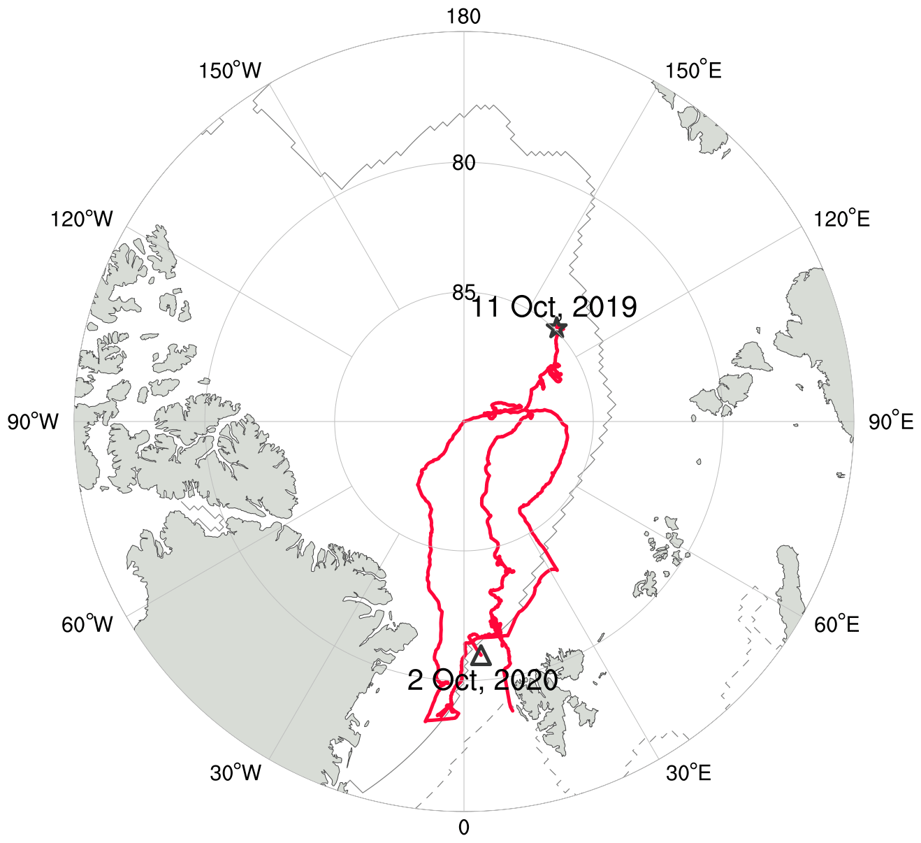
Figure 1The MOSAiC expedition track from (star) 11 October 2019 through to (triangle) 2 October 2020 is shown using the red line. Solid and dashed gray lines denote the approximate sea-ice edge at the minimum (15 September 2020) and the maximum (5 March 2020), respectively.
2.1 Radiosonde observations and relevant data products
The radiosonde data were obtained through a partnership between the leading Alfred Wegener Institute (AWI); the Atmospheric Radiation Measurement (ARM) User Facility, a US Department of Energy (DOE) facility managed by the Biological and Environmental Research program; and the German Weather Service (DWD) (Maturilli et al., 2022). Vaisala RS41-SGP radiosondes were regularly launched on board throughout the whole MOSAiC year (from October 2019 to September 2020), including periods when the vessel was in transit. The sounding frequency is normally four times per day (launched at about 05:00, 11:00, 17:00, and 23:00 UTC) but is increased to seven times per day during periods of exceptional weather or coordination with other observational activities. The radiosoundings provide data on the atmospheric state, including vertical profiles of pressure, temperature, relative humidity (RH), and winds, from 12 m up to 30 km with a vertical resolution of 5 m. However, the sounding data below ∼ 100 m altitude may be contaminated by the vessel itself. To avoid contamination affecting our analysis, we use a merged data product that combines the soundings with measurements from a meteorological tower on the sea ice away from the vessel; the abovementioned merged product was specifically designed to minimize ship effects and provide more reliable profiles in the lowest 100 m, and it will be made available on PANGAEA (Dahlke et al., 2023). In this paper, data quality control and a six-point moving average in height are applied to the merged profile data to eliminate invalid data and measurement noise, and all data are interpolated onto a regular vertical grid with 10 m intervals. In total, there are 1484 sounding profiles available. In addition, DOE-ARM provides a “Planetary Boundary Layer Height Value Added Product” (PBLHT VAP; Riihimaki et al., 2019), which uses several different automated algorithms to compute ABLH estimates based on radiosonde profiles. This VAP provides 964 ABLH estimates, and we select 914 samples from these to ensure that the estimates obtained by all algorithms are available.
2.2 Meteorological and turbulence measurements near the surface
Meteorological and turbulence measurements were made from a tower on the sea ice at “Met City”, which was located 300–600 m away from the vessel (Cox et al., 2023). The u-Sonic-3 Cage MP anemometers by METEK GmbH and HMT300 air temperature sensors by Vaisala were fixed at nominal heights of 2, 6, and 10 m on the meteorological tower. The tower was set up during the periods when the vessel passively drifted with an ice floe (i.e., from mid-October 2019 to mid-May 2020, from mid-June through July 2020, and from late August to mid-September 2020). The sampling frequency of fast-response instruments (i.e., u-Sonic-3 Cage MP anemometer) was at 20 Hz, resampled to 10 Hz. To derive turbulence parameters, the following processes were carried out: despiking, block averaging over a 10 min interval, coordinate rotating via double rotation, frequency correcting, and virtual temperature correcting. In this study, sensible heat flux (SH, defined as positive upwards), near-surface air temperature at 2 m, friction velocity, and turbulent kinetic energy (TKE) dissipation rate are used. Based on a footprint analysis using the Kljun et al. (2015) model, 90 % of the sensible heat flux measurements have a source area fetch of no more than 275 m, a region that was typically dominated by consistent sea ice throughout the year. Although the sounding site may typically be outside the source region of these flux measurements, we assume that the conditions at the two sites are equivalent, which is also assumed in the merged sounding–tower product.
2.3 Cloud properties derived from combined sensors
Cloud-related measurements come from the ShupeTurner cloud microphysics product (Shupe, 2022). This product uses multiple measurement sources (e.g., cloud radar, ceilometer, depolarization lidar, and microwave radiometer) to derive time–height data, including cloud-phase type and condensed water content for both liquid and ice. Details of the retrieval algorithm, its application, and uncertainties are provided in Shupe et al. (2015). In our study, the condensed water content data are linearly interpolated onto the vertical grid with a resolution of 10 m for consistency. The cloud-phase-type data are used to determine clear and cloudy environments. A grid point is labeled as “cloudy” if clouds are identified in the upper and lower cloud-phase-type data points adjacent to the grid; otherwise, the grid point is labeled as “clear”.
The most objective method of ABLH determination is based on profiles of turbulence measurements deployed on aircraft or other platforms, but such measurements were not routinely carried out during the MOSAiC expedition. Thus, the ABLH determination in our study is based on the thermal and dynamic structure of radiosoundings. In previous literature, the ABLH is determined through multiple profiles of atmospheric variables and manual visual inspection, which can be considered as the “observed” ABLH (Liu and Liang, 2010; Zhang et al., 2014; Jozef et al., 2022). In this section, we will describe the manually labeled ABLH determination method and derive an ABLH for each sounding. Next, we will use these ABLHs as a reference to evaluate the automated ABLH algorithms provided by the PBLHT VAP. Finally, we will develop and evaluate an improved ABLH automated algorithm that is suitable for the Arctic atmosphere and further discuss an important parameter for the algorithms and its stability dependence.
3.1 ABL regime classification and ABLH determination
The ABLH determination method starts with the classification of ABL regimes. Based on previous studies (e.g., Vogelezang and Holtslag, 1996; Liu and Liang, 2010), we divide the ABLs into three types corresponding to three different stability states near the surface: stable boundary layer (SBL), near-neutral boundary layer (NBL), and convective boundary layer (CBL). We first use SH to diagnose the ABL regime types. The specific classification formula is presented below:
where δ is the critical value that is specified as 2 W m−2, following Steeneveld et al. (2007b). If corresponding SH data are unavailable, the difference in the equivalent potential temperature (θE) between the 100 and 50 m heights (θE difference) derived from the sounding profile is used to determine the ABL type. Specifically, if the θE difference is larger than 0.2 K, the ABL is identified as SBL; if the θE difference is less than −0.2 K, the ABL is identified as CBL; and other profiles are labeled as NBLs, roughly following Liu and Liang (2010).
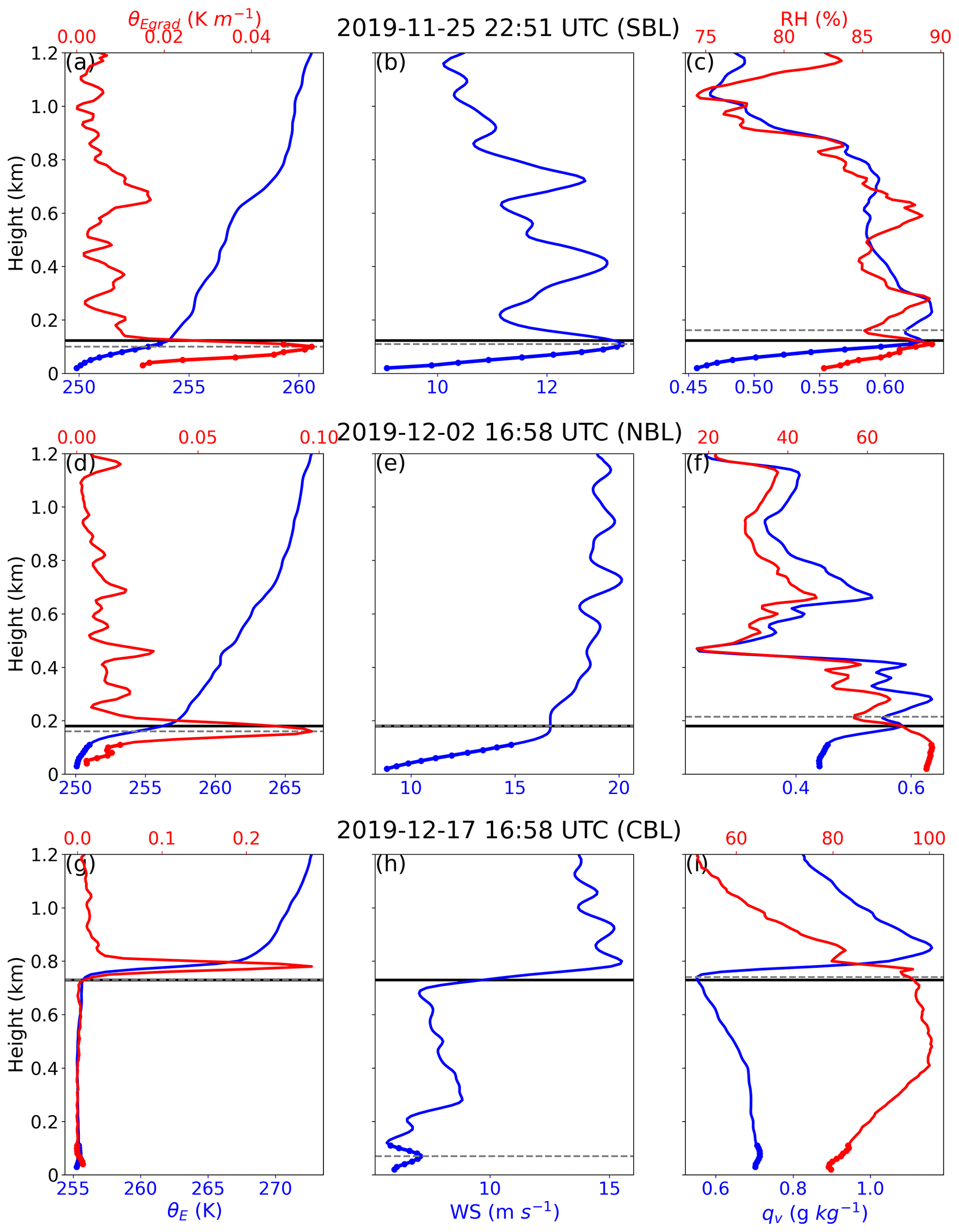
Figure 2Vertical profiles of (a, d, g) equivalent potential temperature (θE), equivalent potential temperature gradients (θEgrad), (b, e, h) wind speed (WS), and (c, f, i) relative humidity (RH) and specific humidity (qv) on (a–c) 25 November 2019 at 22:51 UTC, (d–f) 2 December 2019 at 16:58 UTC, and (g–i) 17 December 2019 at 16:58 UTC. Boundary layers at the three aforementioned times represent a stable boundary layer (SBL), a near-neutral boundary layer (NBL), and a convective boundary layer (CBL), respectively. The dashed horizontal gray lines denote the atmospheric boundary layer height (ABLH) estimates based only on the profile shown in that panel, and the solid horizontal black lines denote the manually observed ABLHs. The dots in the lowest 100 m denote the section of the profiles impacted by the radiosonde–tower merging.
The manually labeled ABLH determination in our study is based on characteristics of sounding profiles and regime types. For each atmospheric sounding profile, equivalent potential temperature (θE), equivalent potential temperature gradient (θEgrad), wind speed (WS), specific humidity (qv), and RH are used to obtain multiple estimates of the ABLH, which are used to determine the final estimate. Three cases to describe the method are presented in Fig. 2. Figure 2a, b, and c illustrate the case of an SBL, which features surface-based temperature and humidity inversions. Figure 2d, e, and f show the case of an NBL, with approximately constant θE from the surface up to the inversion base and strong horizontal wind. Figure 2g, h, and i present the case of a CBL, with a deeper well-mixed layer and low-level cloud coupled to the surface (e.g., Shupe et al., 2013). In terms of θE profiles, the estimated ABLH is the level at which the θEgrad reaches its maximum for SBL and NBL cases, whereas it is the level at which it reaches the base of the θE inversion for CBL cases (Martucci et al., 2007). In terms of WS profiles, the ABLH is estimated to be the height of the WS maximum for all three regime types (Mahrt et al., 1979). In terms of humidity profiles, the estimated ABLH is the level at which the RH rapidly decreases for SBL and NBL cases, whereas it is the base of the qv inversion for CBL cases (Lenschow et al., 2000). The manually observed ABLHs (solid black lines in Fig. 2) are then determined via the consideration of these three distinct estimates using the following rules: (1) if the estimates differ slightly from each other, take the average of these estimates as the ABLH; (2) if a strong characteristic (sharp gradients or peaks) of the profile is evident, select the estimate obtained based on this characteristic; (3) if the ABL structure is similar to that at the previous time, select the estimate with the smallest change to ensure that the ABLHs are consistent in time. It is evident that the lowest layers of profiles have a great impact on the ABLH determination, particularly for shallow SBLs and NBLs. Thus, the merged radiosonde–tower profiles help make the ABLH determination more reliable than when using radiosondes alone.
3.2 Automated algorithm evaluation
The automated ABLH algorithms consist of various empirical formulas. Based on these empirical formulas, estimated ABLHs are determined automatically and without manual intervention. Therefore, these algorithms can perform real-time and fast calculations on large amounts of data and are widely used in model simulations (Seibert et al., 2000; Konor et al., 2009). However, automated algorithms might lead to large errors in estimating ABLHs, and the parameter selection in these algorithms will have a great impact on the results. In our study, estimated ABLHs obtained using three automated algorithms are compared with manually labeled ABLHs to evaluate their performance over the Arctic Ocean. These algorithms, including the Liu–Liang algorithm, the Heffter algorithm, and the bulk Richardson number algorithm, are all available in the PBLHT VAP, as described in Sivaraman et al. (2013). Here, we give a brief description of the three algorithms.
The Liu–Liang algorithm determines the ABLH based on potential temperature and wind speed according to Liu and Liang (2010). For CBL regimes, the definition of the ABLH is the height at “which an air parcel rising adiabatically from the surface becomes neutrally buoyant” and the temperature excess value is 0.1 K. For SBL regimes, two different estimates of the ABLH are obtained, if possible, based on stability criteria and wind shear criteria, respectively. For stability, the ABLH is defined as the lowest level, k, at which the θEgrad reaches a minimum and meets either of the following two conditions:
where the subscripts (k, k−1, k+1, and k+2) represent the θEgrad at corresponding levels. For wind shear, the ABLH is defined as the height at which the wind speed reaches a maximum that is at least 2 m s−1 stronger than the layers immediately above and below while decreasing monotonically toward the surface (i.e., a low-level jet). The final ABLH is defined as the lower of the two heights.
The Heffter algorithm, which was suggested by Heffter (1980), is a widely used algorithm (e.g., Marsik et al., 1995; Snyder and Strawbridge, 2004). The algorithm determines the ABLH through the strength of the inversion and potential temperature difference across the inversion. The ABLH is defined as the lowest layer in which the potential temperature difference between the top and bottom of the inversion is greater than 2 K. If no layer meets the criteria, the ABLH is defined as the layer at which the potential temperature gradient reaches the largest maximum.
The bulk Richardson number algorithm is based on the profile of the bulk Richardson number (Rib) and has been shown to be a reliable algorithm for determining ABLHs (Seidel et al., 2012). Rib is a dimensionless number that represents the ratio of thermally produced turbulence to that induced by mechanical shear. The Rib formula used in the PBLHT VAP (Sørensen et al., 1998; Sivaraman et al., 2013) is expressed as follows:
where g is the acceleration of gravity; θvh and θv0 are the virtual potential temperature at height h and the surface, respectively; and uh and vh are the horizontal wind speed components at height h. The ABLH is defined as the height of Rib exceeding a critical threshold (the critical bulk Richardson number, Ribc; Seibert et al., 2000). The PBLHT VAP includes ABLH estimates based on two widely used Ribc values: 0.25 and 0.5.
To quantitatively evaluate the performance of each automatic algorithm, we introduce the correlation coefficient R and two other statistical measures: the dimensionless Bias and the median absolute error (MEAE; Steeneveld et al., 2007a). The formulas for these measures are as follows:
where Hauto is the ABLH obtained by the automated algorithm, Hobs is the manually determined ABLH, and n is the number of valid sounding profile samples. According to the definitions of these statistical measures, larger R and smaller Bias and MEAE mean a better performance of the automated algorithm.
We also analyze the algorithms' performance for cloudy and clear conditions, considering that low-level clouds containing liquid water play an important role in the Arctic ABL (Shupe and Intrieri, 2004; Brooks et al., 2017). In our study, the RH threshold of 96 % (Silber and Shupe, 2022) and the cloud source flag data are used for cloud detection. If a cloud is detected in the cloud source flag data and the RH is higher than 96 %, the profile is labeled as cloudy. The sounding profiles that contain at least one identified cloud layer below 1500 m are classified as cloudy; otherwise, they are classified as clear.
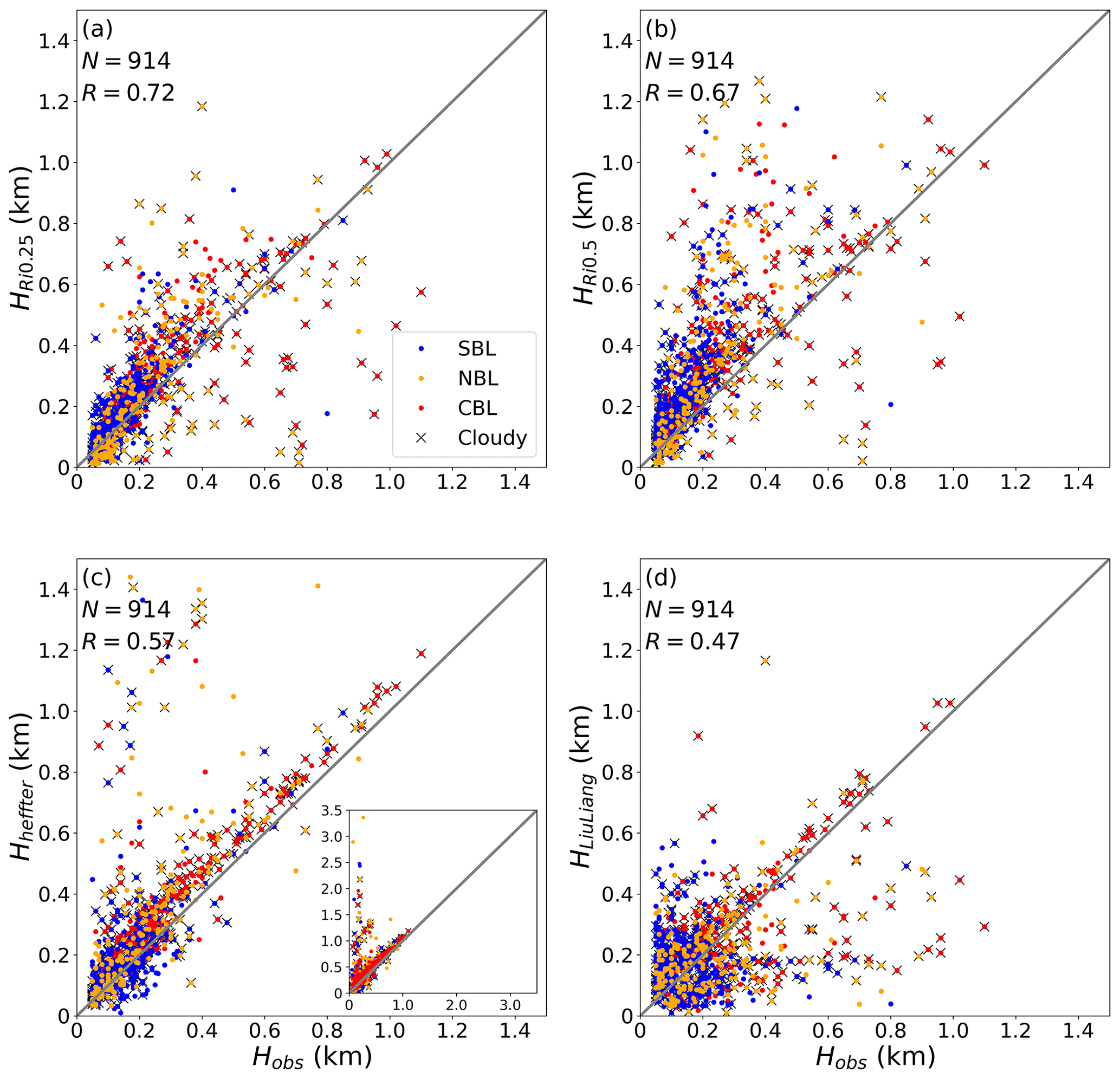
Figure 3Comparisons of the ABLHs determined from radiosonde profiles using the bulk Richardson number (Rib) algorithm with the critical values (Ribc) of (a) 0.25 and (b) 0.5, (c) the Heffter algorithm, and (d) the Liu–Liang algorithm with the manually identified “observed” ABLHs. The blue, yellow, and red colors indicate SBL, NBL, and CBL regime types, respectively. The “x” markers indicate cloudy ABLs. The case numbers (N) and correlation coefficients (R) are given in each panel. The inset in panel (c) denotes all data points ranging from 0 to 3.5 km.
Table 1The statistical measures (R, Bias, and MEAE) for the four algorithms applied to the radiosonde dataset. All correlation coefficients are statistically significant (p < 0.05), except for SBL types in the Liu–Liang algorithm.
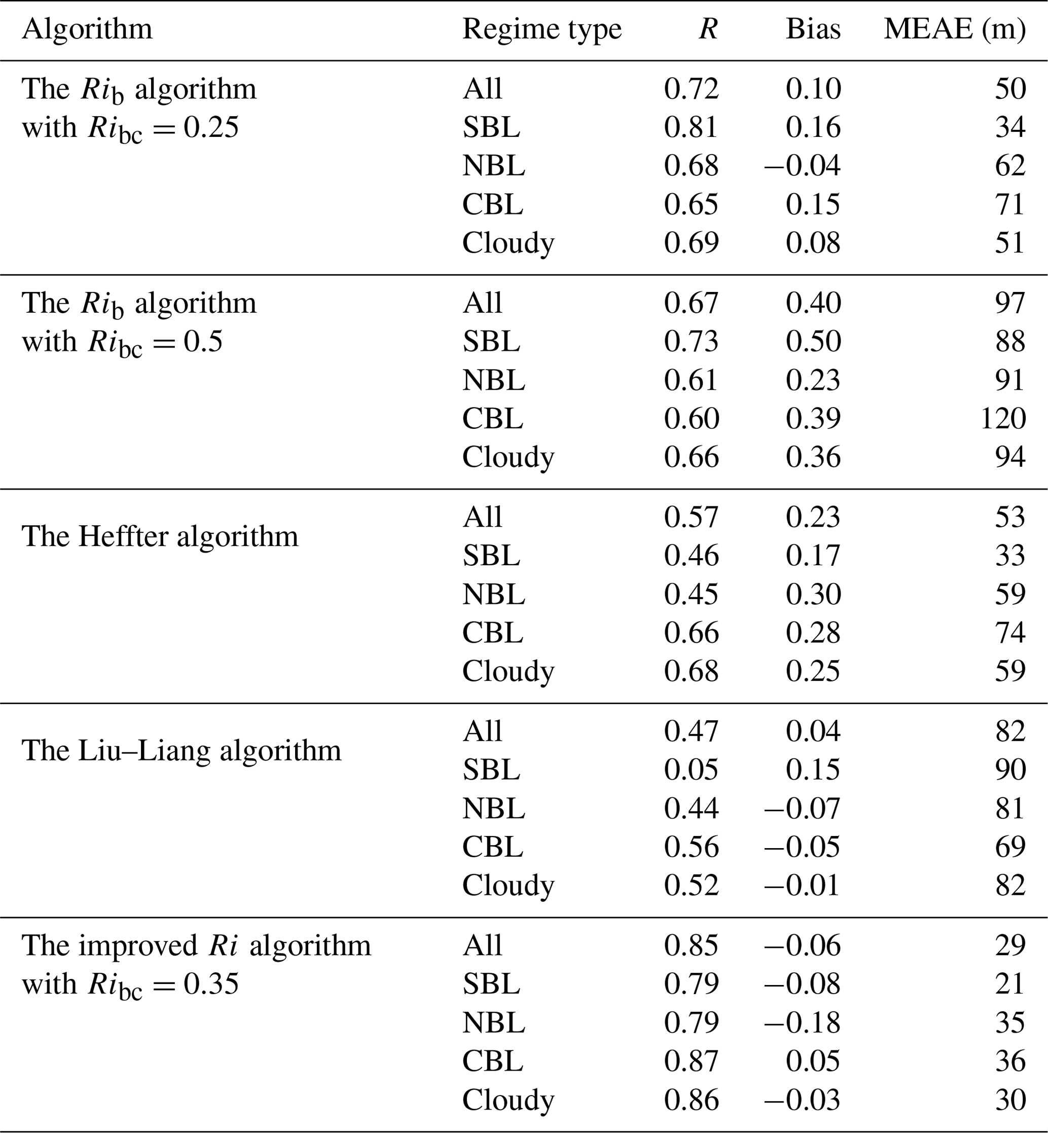
Figure 3 presents the comparisons of estimated ABLHs with the manually labeled ABLHs, and the associated statistical measures are given in Table 1. The results show that the Rib algorithm with an Ribc of 0.25 performs best overall, particularly for SBL cases. The performance of the Rib algorithm with an Ribc of 0.5 is poorer than that of the Rib algorithm with an Ribc of 0.25, with overestimations of the ABLHs in general as well as larger errors with lower correlation coefficients for all types of ABLs. The Heffter algorithm performs well in cases with a high ABLH and particularly for cloudy and CBL cases, but it does significantly overestimate the ABLH in a large number of cases, as shown in the inset in Fig. 3c. This is attributed to the determination criterion of the Heffter algorithm, i.e., ABLHs are determined by inversion layers, which means that large errors occur when the inversion layer is higher than the mixed layer. Additionally, while the Heffter algorithm's performance under many of the ABL conditions is only marginally worse statistically than the Rib algorithm with an Ribc of 0.25, its correlations are notably worse for SBL and NBL cases. The performance of the Liu–Liang algorithm is generally poorer than the other algorithms, particularly with respect to the correlation coefficient, which is probably due to the impact of noise in the lower ABLH profiles and unsuitable parameters in the algorithm. In summary, the Rib algorithm is reliable over the Arctic Ocean and performs better than other algorithms, and this result agrees with Jozef et al. (2022). Furthermore, we will explore ways to improve the Rib algorithm to make it more suitable for cloudy and convective conditions.
3.3 An improved Ri algorithm considering the cloud effect
As a traditional Rib formula, Eq. (3) may break down in cases with ABLs with a relatively high wind speed and upper-level stratification due to the overestimation of shear production (Kim and Mahrt, 1992). Vogelezang and Holtslag (1996) proposed a finite-difference Ri formula, which is expressed as follows:
where zs is the lower boundary for the ABL; θvs, us, and vs are the θv and wind components at the height zs, respectively; b is an empirical coefficient; and u∗ is the surface friction velocity. RiF is considered for a parcel located somewhat above the surface to avoid the above problem, and u∗ is also taken into account to avoid underestimation in the situation of a uniform wind profile in the upper layer. Here, we use RiF for clear-sky profiles and take zs and b values of 40 m and 100, respectively, according to Zhang et al. (2020).
As shown in Fig. 3, the estimations of cloudy ABLHs are sometimes quite poor, which motivates us to further improve the algorithm. Under cloudy conditions, the moist Richardson number (Rim) can be used to include cloud effects on the buoyancy term. Brooks et al. (2017) adopted the Rim formula that is expressed as follows:
where T is air temperature, Γm is the moist adiabatic lapse rate, L is the latent heat of vaporization, qs is the saturation mixing ratio, and qw is the total water mixing ratio (i.e., , where qL is the liquid water mixing ratio and is obtained based on the condensed water content). However, Eq. (7) is a gradient Ri and is calculated based on local gradients of wind speed, temperature, and humidity. To be consistent with the Ri formula proposed by Vogelezang and Holtslag (1996), we rewrite the formula in a finite-difference form that is expressed as follows:
where the subscripts (h and s) of the variables denote the calculated height, similar to Eq. (6); however, it should be noted that s and zs are adjusted to 130 m, given the cloud radar blind zone. Considering that Rim is only appropriate for the liquid-bearing-cloud cases, we use RiF for clear grid points and Rim for cloudy grid cells. Using this improved approach, we evaluated the best value of Ric to minimize the errors compared to the reference dataset, arriving at an optimal value of Ric=0.35. The comparison of ABLH estimates obtained through the improved Ri algorithm with the manually labeled ABLHs demonstrates significant improvement relative to other algorithms, particularly for cloudy conditions (Fig. 4, Table 1).
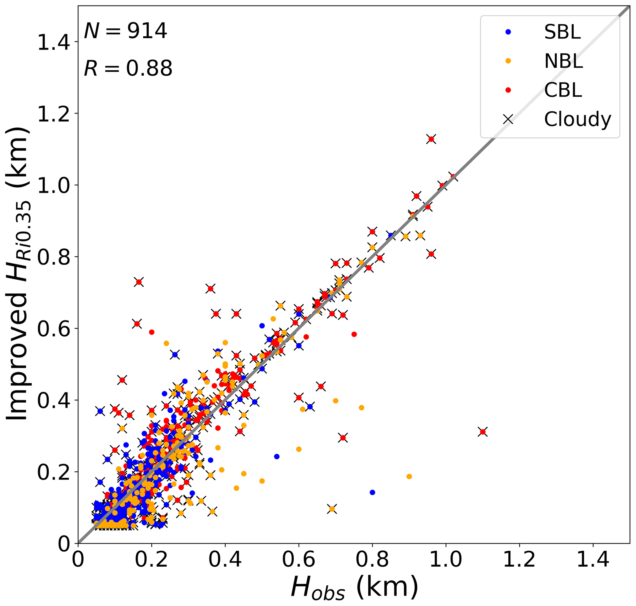
Figure 4Similar to Fig. 3 but for the comparison of the ABLHs determined by the improved Ri algorithm with the observed ABLHs. The case number (N) and correlation coefficient (R) are given.
As some other studies have proposed different Ric values for MOSAiC (e.g., Jozef et al., 2022; Barten et al., 2023; Akansu et al., 2023), we will discuss the difference in Ric values here. The first thing to make clear is that these studies use different formulas to obtain Ri profiles. Barten et al. (2023) and Akansu et al. (2023) both used the traditional Rib algorithm based on Eq. (3), but they used Ric values of 0.4 and 0.12, respectively. This difference was likely caused by the different methods employed to manually derive their reference ABLH datasets. Jozef et al. (2022) calculated the Ri over a rolling 30 m altitude range, labeled as Rir, and the criterion was modified to require four consecutive data points to be above the Ric of 0.75. In our study, we use RiF proposed by Vogelezang and Holtslag (1996) for clear-sky conditions, and we utilize Rim for cloudy conditions. Based on the results presented here, it is apparent that this more complex approach improves the error statistics relative to approaches based on Eq. (3). In addition, some of the differences may also be related to authors using different datasets or time periods. For instance, Akansu et al. (2023) primarily used sounding data based on a tether balloon for a specific subperiod of MOSAiC, whereas Jozef et al. (2022) used radiosondes from periods for which they had concurrent UAV observations. The data used in our study are based on a merged sounding–tower product, as mentioned above.
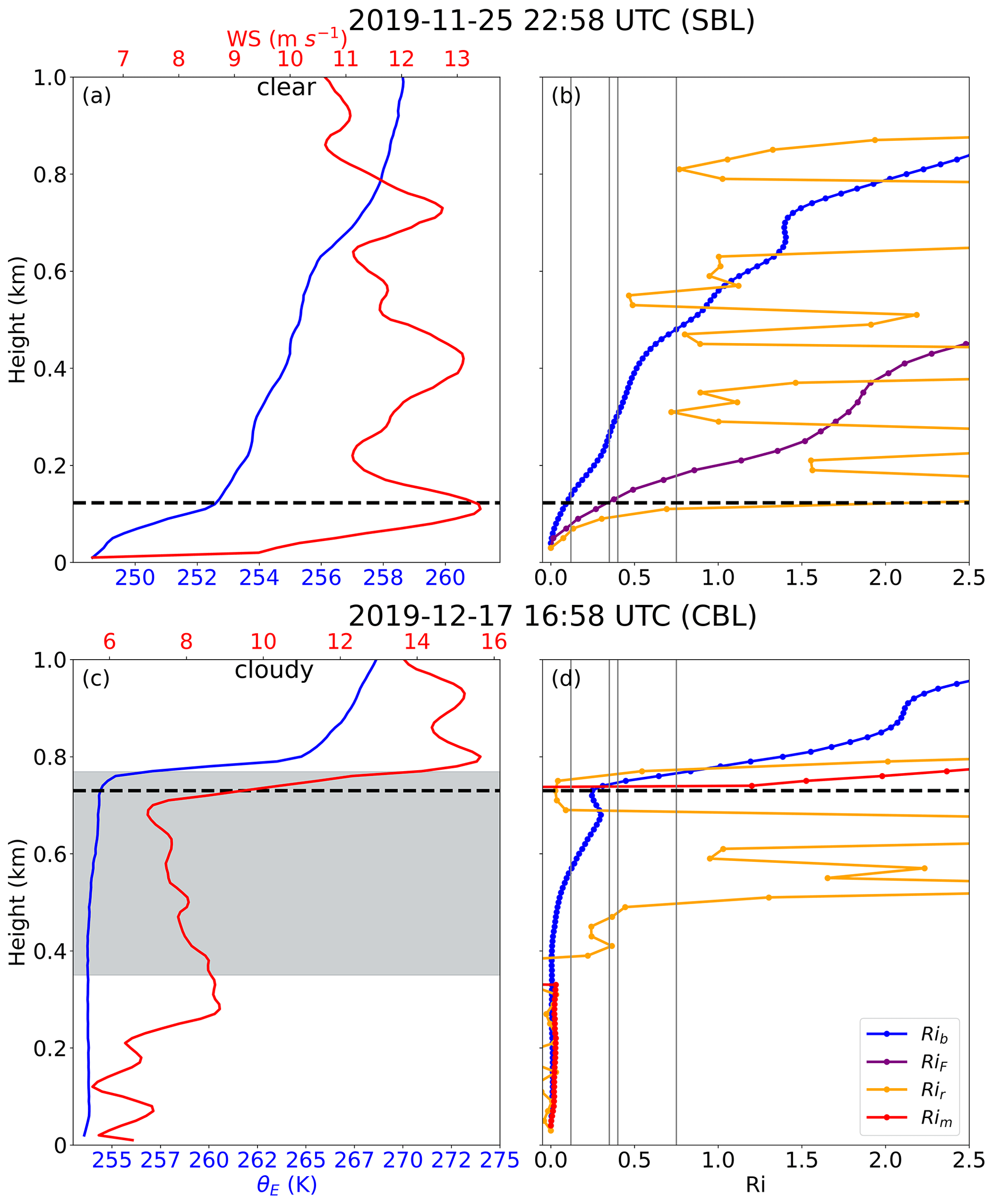
Figure 5Vertical profiles of (a, c) θE and wind speed and of (b, d) Ri based on different formulas on (a–b) 25 November 2019 at 22:58 UTC and (c–d) 17 December 2019 at 16:58 UTC. Boundary layers at the two times represent a clear-sky SBL and a cloudy-sky CBL, respectively. The dashed horizontal black lines denote the manually identified ABLH, and the solid vertical gray lines denote the different Ric values, including 0.12, 0.35, 0.4, and 0.75. The gray shading in panel (c) denotes the cloud layer.
To further explore the differences among the four different approaches, we examine one SBL and CBL case. For a clear-sky SBL case (Fig. 5a, b), the approaches from Akansu et al. (2023), Jozef et al. (2022), and this study all agree closely with the manual ABLH, whereas the Barten et al. (2023) approach results in a significant overestimation. For a cloudy-sky CBL case (Fig. 5c, d), the approach from this study agrees with the manual ABLH, whereas the approach from Barten et al. (2023) overestimates the ABLH by about 30 m and the approaches from Akansu et al. (2023) and Jozef et al. (2022) underestimate the ABLH by 130 and 230 m, respectively. These results further demonstrate how Ric depends on the choice of the Ri formula. Moreover, Ric is not analytically derived from basic physical principles (Zilitinkevich et al., 2007), and the concept of Ric is challenged by nonsteady regimes (Zilitinkevich and Baklanov, 2002) and the hysteresis phenomenon (Banta et al., 2003; Tjernström et al., 2009). Therefore, an objective Ric does not exist; rather, it is empirically used as an algorithmic parameter to simply derive the ABLH.
3.4 The stability dependence of the critical Richardson number
Richardson et al. (2013) and Basu et al. (2014) suggested that there is a stability dependence of Ric under stable conditions, which is different from the constant Ric=0.35 used in our improved algorithm. In this section, we will discuss the impact of this dependence on the ABLH estimation. We use the improved Ri algorithm to calculate the Ri at the manually labeled ABLH (h). This new parameter is named Rih to distinguish it from the constant Ric. To be consistent with Basu et al. (2014), the bulk stability parameter is used for our analysis, where L is the Obukhov length at the surface. Based on these two variables, the stability dependence can be expressed as follows:
where α is a proportionality constant. As suggested in Basu et al. (2014), the data for convective, near-neutral, and very stable conditions are excluded to obtain a credible α. Specifically, data points that meet the thresholds (L > 500 m and L < Lmin) are excluded in our analysis, where the Lmin corresponds to the heat flux minimum (Basu et al., 2008) and is assumed to be 20 m here. Finally, we select 168 samples. The Rih plotted as a function of for these selected data is presented in Fig. 6, and the value of L is colored to probe if the dependence is simply due to self-correlation. The results show Rih values that mostly range from 0 to 0.75, and the best-fit line indicates an overall positive correlation trend, with α=0.11. The α value is somewhat larger than the results in Richardson et al. (2013) and Basu et al. (2014), which is attributed to the different Ri algorithm used in our study. In addition, if a few of the extreme points are removed, the bulk of the data does not show a strong dependence and is instead fairly well represented by a constant Rih = 0.35, which is also suitable for convective conditions (e.g., Fig. 5c and d).
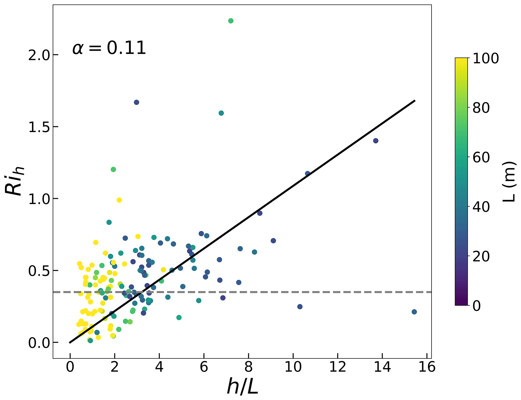
Figure 6Rih versus for selected cases. The data points are colored based on the value of L. The solid black line is the best fit for the selected data points, and the best-fit α value is also given. The gray dashed line is the constant Ric = 0.35 used in the improved Ri algorithm.
In summary, we assess the stability dependence of Ric based on our improved Ri algorithm, and the results present an overall positive correlation trend. However, this type of stability dependence of Ric is challenging to use in practical applications because the sensitivity of α to surface characteristics and atmospheric conditions can additionally degrade the accuracy of ABLH estimates. In addition, Eq. (9) requires a priori determination of the ABLH, which also causes difficulties with respect to the practical application of such an approach. Therefore, we still use the Ri algorithm with a fixed Ric = 0.35 for simplicity.
4.1 Overall distribution of the ABLH
In this section, we analyze the ABLH variation during the MOSAiC expedition as well as relevant controlling factors, based on the manually labeled ABLH dataset and the ABL types that are determined via Eq. (1), or only the θE difference if SH is unavailable. The full time series of the ABLH during the MOSAiC expedition is presented in Fig. 7 and forms the basis for the remaining analyses. According to near-surface conditions and the sea-ice state, the whole MOSAiC observation period is divided into “freeze-up”, “winter”, “transition”, and “summer melt” periods (Shupe et al., 2022), roughly corresponding to the seasons of autumn, winter, spring, and summer, respectively. In Fig. 7, the solid black lines indicate persistent low-level clouds that exist for more than 12 h; these occur most frequently in the late summer and autumn (the freeze-up period), which agrees with Shupe et al. (2011). Note that the gray dots indicate that the ABL data were observed while the vessel was in transit, and the representativity of the ABLH data should be considered in this context. For the first such period, the vessel left the MOSAiC ice floe in mid-May and slowly progressed south through tightly consolidated sea ice, such that the data are generally representative of the sea-ice pack in the region. Measurements from early June when the vessel was near or in open water close to Svalbard have been excluded entirely from the analysis. In the middle of June, as the vessel returned to the original MOSAiC ice floe, the sea ice was not as tightly consolidated and the vessel preferentially went through leads; the preferentially lower ice fraction along this transit could have impacted the thermal structure of the ABL. For the 3 weeks in early August, the vessel moved around in the Fram Strait area and then made its way north to another passive sea-ice drifting position near the North Pole, again transiting through regions with lower sea-ice fraction. Finally, at the very end of the expedition, the vessel took some time to exit the sea ice, stopping a few times to allow for work on the ice.
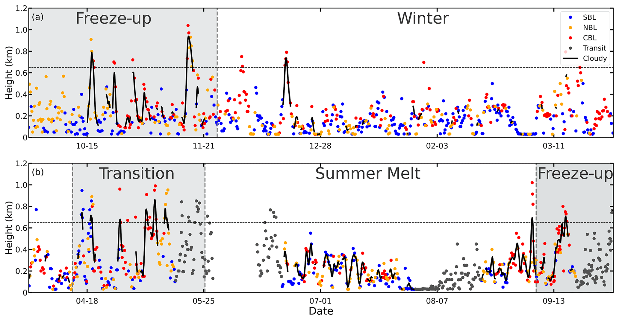
Figure 7The time series of ABLHs throughout the MOSAiC year is divided into panels (a) and (b). The blue, yellow, and red dots indicate the SBL, NBL, and CBL heights, respectively. The gray dots indicate ABL data observed while the vessel was in transit. The solid black lines indicate the heights of cloudy ABLs that persist for at least 12 h. The dashed horizontal gray line denotes the 95th percentile of the ABLH (650 m). The gray and white shaded background areas indicate the periods under different surface-melting states, i.e., the freeze-up, winter, transition, and summer melt periods.
Overall, as shown in Fig. 7, the mean ABLH during the whole observation period is 231 m. This is lower than the typical ABLH over the Arctic land surface (Liu and Liang, 2010), which is primarily attributed to the stronger suppression of the temperature inversion over the sea-ice surface. The Arctic ABL is suppressed for most of the MOSAiC year, although it intensively develops for several days at a time, most commonly when clouds and a CBL are present, for a few periods. For instance, frequent, intensive ABL development occurs in the transition period from 13 April through to 24 May 2020. In this period, the convective thermal structure and cloud effects contribute to the ABLH reaching over the 95th percentile of the ABLH data (horizontal dotted line) for about 7 d, with a maximum ABLH of 1100 m. In contrast, the ABL is strongly suppressed in the period from 15 July through to 30 August 2020, with a mean ABLH of only 136 m. The specific mechanisms of ABL development and suppression in these two cases will be analyzed in Sect. 4.3 and 4.4, respectively.
Figure 8 presents the frequency distribution of the ABLH under SBL, NBL, and CBL regime types. Overall, the sample number of SBL cases is more than that of NBL and CBL cases during the MOSAiC period (43 % for SBL, 31 % for NBL, and 26 % for CBL). These occurrence frequencies roughly agree with Jozef et al. (2023), although their results show more NBL and CBL and less SBL. This is likely to be attributed to differences in the classification criteria. The distributions of SBL and NBL ABLHs are skewed towards small values, with 94 % and 79 % of the ABLH values lower than 400 m, and mean values of 165 and 256 m, respectively. For CBL, the distribution is shifted somewhat towards larger values, with 23 % of the ABLH values higher than 600 m and a mean value of 309 m.
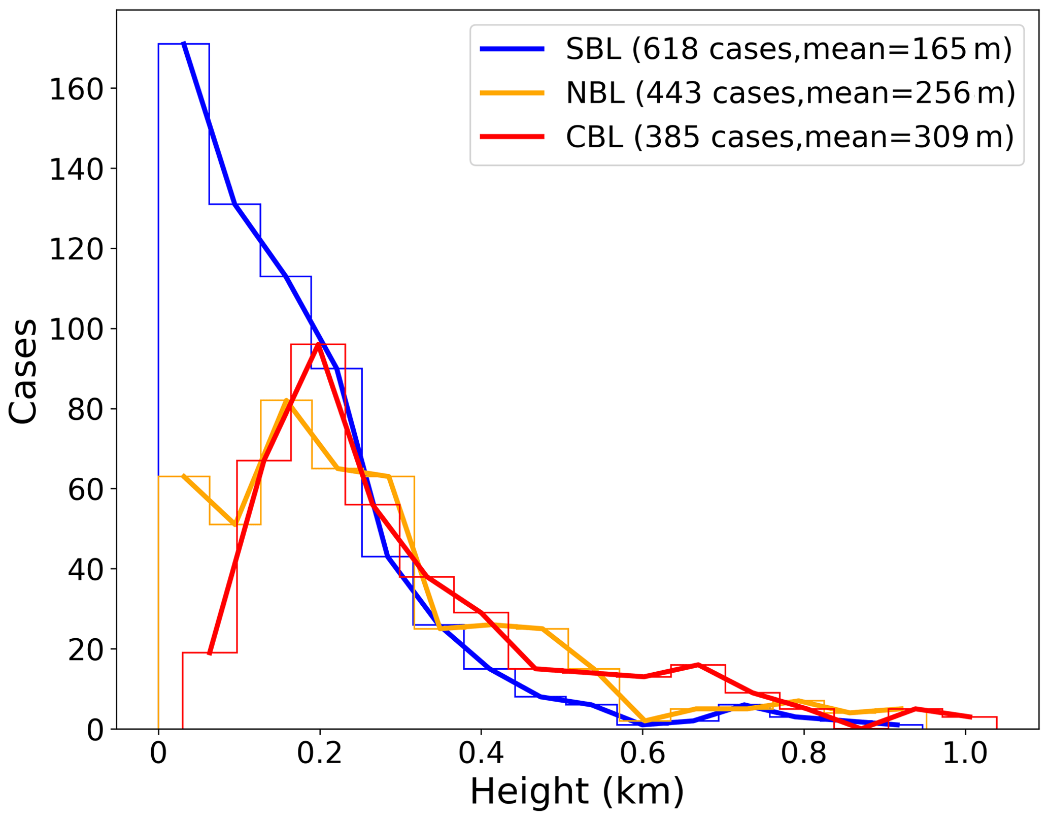
Figure 8Frequency distribution of SBL height (blue), NBL height (yellow), and CBL height (red). The case numbers and the mean values of the ABLH for SBL, NBL, and CBL conditions are also given.
4.2 Annual cycle of the ABLH and related factors
Figure 9 presents the annual cycle of the monthly ABLH statistics during the MOSAiC expedition in terms of the 5th, 25th, 50th, 75th, and 95th percentiles of the ABLH (box plots) and the mean value (“x” markers and solid and dashed lines). The box-and-whisker plots show a distinct peak in May, with a median value of 363 m and the 95th percentile reaching over 800 m. An abrupt decrease occurs in the following July and August, and another minimum occurs in January, all with median values below 150 m. It should be noted that the ABLH data in transit (gray dots in Fig. 7), which could have been potentially impacted by more open-surface water conditions, are also included in the statistics. Specifically, the ABLH data during transit periods cause a higher mean ABLH for June and a lower mean ABLH for August (see Fig. 7). The comparison between cloudy and clear-sky ABLHs indicates that the low-level clouds significantly contribute to the Arctic ABL development during the MOSAiC year, except in winter, when low-level clouds are rare.
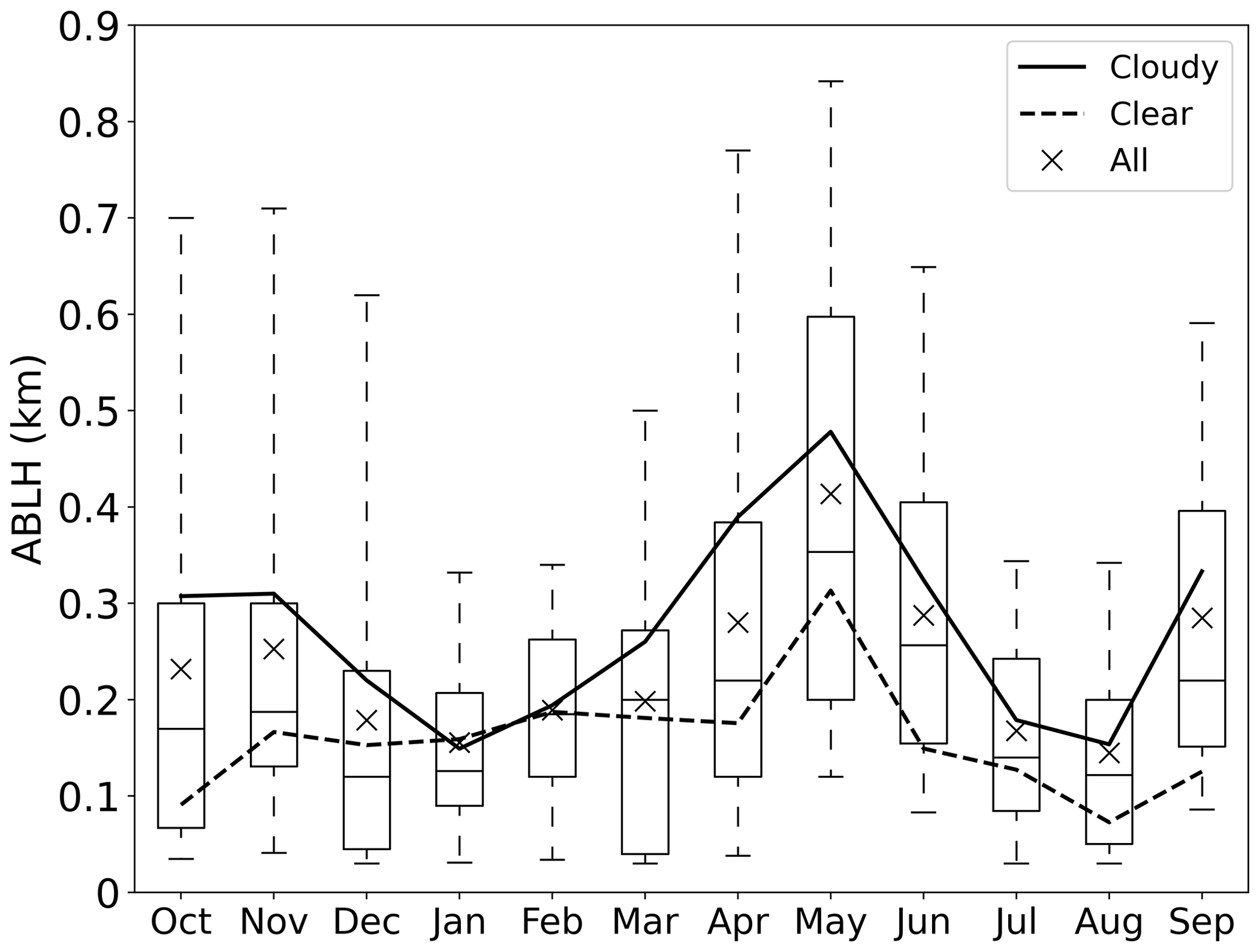
Figure 9Box-and-whisker plots of the ABLH distribution in each month throughout the MOSAiC year. The whiskers, the boxes, and the horizontal black lines show the 5th, 25th, 50th, 75th, and 95th percentile values of the ABLH. The solid and dashed lines and the “x” markers indicate the mean ABLH of cloudy, clear, and all ABL types, respectively.
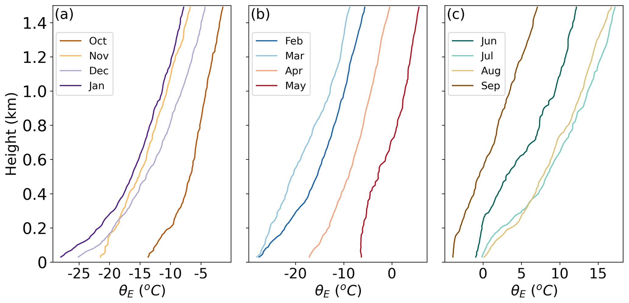
Figure 10Monthly median profiles of equivalent potential temperature throughout the MOSAiC year. Panel (a) represents October–January, panel (b) represents February–May, and panel (c) represents June–September.
The annual cycle of the ABLH is determined by the seasonal evolution of the ABL structure (Tjernström et al., 2009; Palo et al., 2017), as revealed through median profiles of θE in each month (Fig. 10). The results show that, from the start of the MOSAiC expedition (October 2019), the near-surface θE gradually decreases due to seasonal surface radiative cooling in the absence of sunlight, more rapidly than the atmosphere cools, which causes a strong surface temperature inversion. The increasing inversion strength through January leads to a decreasing ABLH into “winter.” In February and March, the surface remains steady while the atmosphere cools more, leading to a diminished temperature inversion strength and a small increase in the ABLH. After March 2020, with the return of sunlight, the θE starts to rise over the whole lower atmosphere, and the near-surface air temperature warms somewhat more than the atmosphere above. This differential warming leads to more frequent near-neutral or convective thermal structures and contributes to a high ABLH during the transition period. In July and August, the upper-layer temperature continues to rise while the near-surface temperature is constrained to ∼ 0∘ due to the melting sea-ice surface, which leads again to a surface inversion and a diminished ABLH during the summer melt period. In September, as the Sun descends to much lower angles, the θE across the whole lower atmosphere starts to drop, with more rapid cooling in the atmosphere relative to the near-surface resulting again in near-neutral or convective thermal structures and an increase in the CBL height during the freeze-up period. The whole process forms these general shifts over the annual cycle. In addition, we examined the potential implications of the diurnal cycle on the ABL thermal structure. Monthly profiles based on different moments of a day were found to show little variability (not shown), such that the impact of the diurnal cycle is minimal.
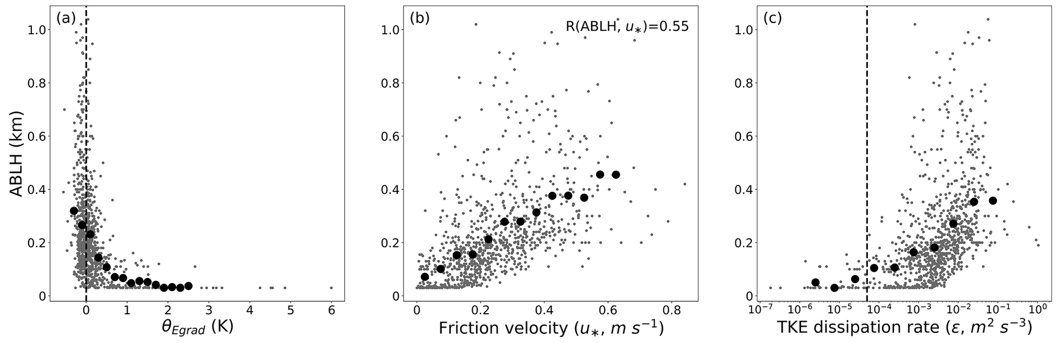
Figure 11The ABLHs and bin-averaged values for (a) equivalent potential temperature gradient, θEgrad (K); (b) friction velocity, u∗ (m s−1); and (c) turbulent kinetic energy dissipation rate, ε (m2 s−3). The average bins for θEgrad, u∗, and ε logarithm are 0.2 K, 0.05 m s−1, and 0.5m2 s−3, respectively. The correlation coefficient R is given in panel (b), which shows statistically significant results (p < 0.05). The dashed vertical lines indicate the thresholds of (a) θEgrad = 0 K and (c) ε = 5 × 10⁻⁵ m2 s−3.
To further explore the relations between surface conditions and the ABLH, we evaluate the correlations between the ABLH and three near-surface meteorological and turbulence parameters during the MOSAiC period, including the near-surface equivalent potential temperature gradient (), friction velocity (u∗), and TKE dissipation rate (ε). The results are shown in Fig. 11. Generally, the near-surface buoyancy and shear effects both modulate these variables. In Fig. 11a, the ABLH distribution for negative θEgrad has a wide range from the lowest level to above 1 km. As θEgrad becomes positive and increases, the ABLH distribution rapidly narrows to below 200 m. In general, positive θEgrad means a stably stratified ABL and surface-based temperature inversion, both of which lead to a low ABLH, and negative θEgrad means that atmospheric stability near the surface is near-neutral or convective, which is necessary for ABL development. The u∗ presents a significant correlation with the ABLH, with correlation coefficient of 0.58 (Fig. 11b). High u∗ values, which are related to strong mechanical mixing, contribute to the ABL development. However, it is worth noting that intensive ABL development (an ABLH over 600 m) only occurs as u∗ ranges between 0.2 and 0.5 m s−1, which suggests that other factors exist to facilitate further development of the ABL, such as cloud effects (see Fig. 9). The ε indicates the rate at which the TKE is changing, and the high value of ε means well-developed turbulence. In Fig. 11c, when ε is less than 5 × 10⁻⁵ m2 s−3, turbulence in the ABL is limited with almost all ABLH values below 200 m. As ε increases and becomes larger than 5 × 10⁻⁵ m2 s−3, the average ABLH increases with active turbulent mixing in the ABL. The threshold of 5 × 10⁻⁵ m2 s−3 was proposed by Brooks et al. (2017) as the distinction between turbulent and nonturbulent flows.
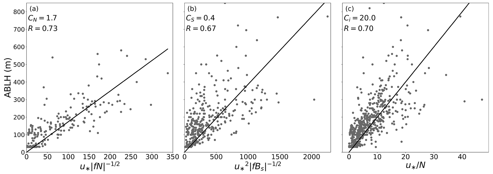
Figure 12The ABLHs versus three expressions in Eqs. (10)–(12). The empirical coefficients CN, CS, and Ci are given in panels (a), (b), and (c), respectively, and represent the slope of the best-fit line (black line). The correlation coefficient R is given in each panel and is statistically significant (p < 0.05).
The free-flow stability (characterized by the free-flow Brunt–Väisälä frequency, N) can affect the ABLH (Zilitinkevich, 2002; Zilitinkevich and Baklanov, 2002; Zilitinkevich and Esau, 2002, 2003) and, therefore, is also examined here. Based on the buoyancy flux at the surface (Bs) and N, the NBLs and SBLs can be further divided into four types: the truly neutral (TN; Bs = 0 and N = 0), the conventionally neutral (CN; Bs = 0 and N > 0), the nocturnal stable (NS; Bs < 0 and N = 0), and the long-lived stable (LS; Bs < 0 and N > 0) boundary layer. According to Zilitinkevich and Baklanov (2002), we calculate the N and Bs and reclassify the SBLs and NBLs. We find that the percentages of N > 0.015 in SBLs and NBLs are 89 % and 80 %, which indicates that LS and CN types dominate the stable and neutral conditions for MOSAiC, respectively. As only 80 TN cases were identified, these are deemed to be too few for additional analysis of this type. Zilitinkevich and Esau (2003) gave ABLH equations relevant to each ABL type as follows:
where hE is the equilibrium ABLH, f is the Coriolis parameter, and CN and CS are empirical coefficients. In addition, Vogelezang and Holtslag (1996) and Steeneveld et al. (2007a) also explore a hE equation without explicitly considering f:
where Ci is an empirical coefficient. Here, we select the CN, NS, and LS ABLH dataset, and fit the data with the corresponding expressions in Eqs. (10)–(12) to obtain the empirical coefficients, and the results are presented in Fig. 12. All three expressions tend to represent the ABLHs well, with significant correlation coefficients. The empirical coefficients CN and CS are 1.7 and 0.4, respectively, which are close to the typical values determined through large-eddy simulations (Zilitinkevich, 2012). The coefficient Ci = 20 in Fig. 12c is double the typical value of 10 (Vogelezang and Holtslag, 1996), but it agrees with the results reported by Overland and Davidson (1992) for the ABL over sea ice. The difference in Ci may be attributed to the unique free-flow stability or other potential mechanisms of ABL development in the Arctic atmosphere.
In summary, near-surface conditions and free-flow stability play a key role in ABL development and are also indicators (in that one can roughly determine the development state of the whole ABL from these basic variables).
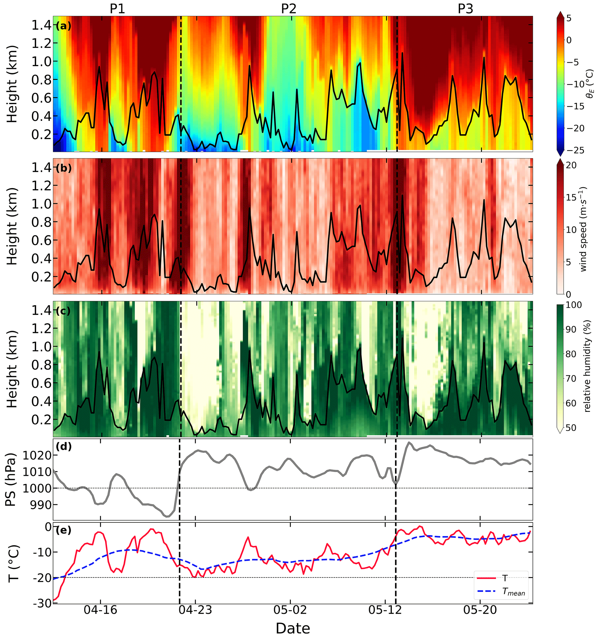
Figure 13Time–height sections of (a) equivalent potential temperature, (b) horizontal wind speed, and (c) relative humidity; time series of (d) surface pressure; and time series of (e) near-surface air temperature (red line) and the 7 d running mean of near-surface temperature (blue line). The whole period is from 13 April 2020 to 24 May 2020. Vertical dashed lines mark the identified periods of P1 to P3. The solid black lines in panels (a)–(c) denote the ABLH during this period.
4.3 Case study no. 1: intensively developed ABL, 13 April–24 May 2020
To investigate the ABL development and its controlling factors, we analyze the association of the ABLH with the vertical thermal structure and near-surface conditions during the transition period (see Fig. 7) when the ABLH was generally the highest. Figure 13 presents time–height cross sections of θE, wind speed, and RH as well as the time series of near-surface temperature and surface pressure during this period. We divide the whole period into three parts based on the ABLH and the vertical structure of the lower troposphere. Overall, the near-surface temperature is generally warmer than −20 ∘C and shows gradual warming towards the melting point. In Period 1 (P1), a warm- and moist-air advection event affects the measurement area, resulting in an increased air temperature, near-saturated RH, strong winds throughout the lower troposphere, and low surface pressure. The approximately constant θE profile near the surface facilitates exchange between the upper and lower layers, and the high-speed wind profile enhances mechanical mixing, leading to a highly developed ABL and ABLH exceeding 600 m. In Period 2 (P2), the near-surface air temperature drops again to between −20 and −10 ∘C, which causes a temperature inversion and partially suppresses the ABL development. However, periodic layers of near-saturated RH extending up to 600 m or more indicate the presence of clouds. The ABLH at these times is related to the depth of the near-saturated layer, consistent with a structure in which the cloud-induced mixed layer aloft couples with the near-surface mixed layer, forming a deeper ABL and higher ABLH (Wang et al., 2001; Shupe et al., 2013). In Period 3 (P3), a high-pressure synoptic system occurs and suppresses the development of the ABL, but cloud-driven turbulent mixing still exists and counteracts the influence of the high-pressure system. In summary, the development of the ABL mainly depends on large-scale synoptic processes, especially warm-air advection events. Additionally, the interaction between the surface-mixed layer and cloud-mixed layer also plays a significant role in the ABL development.
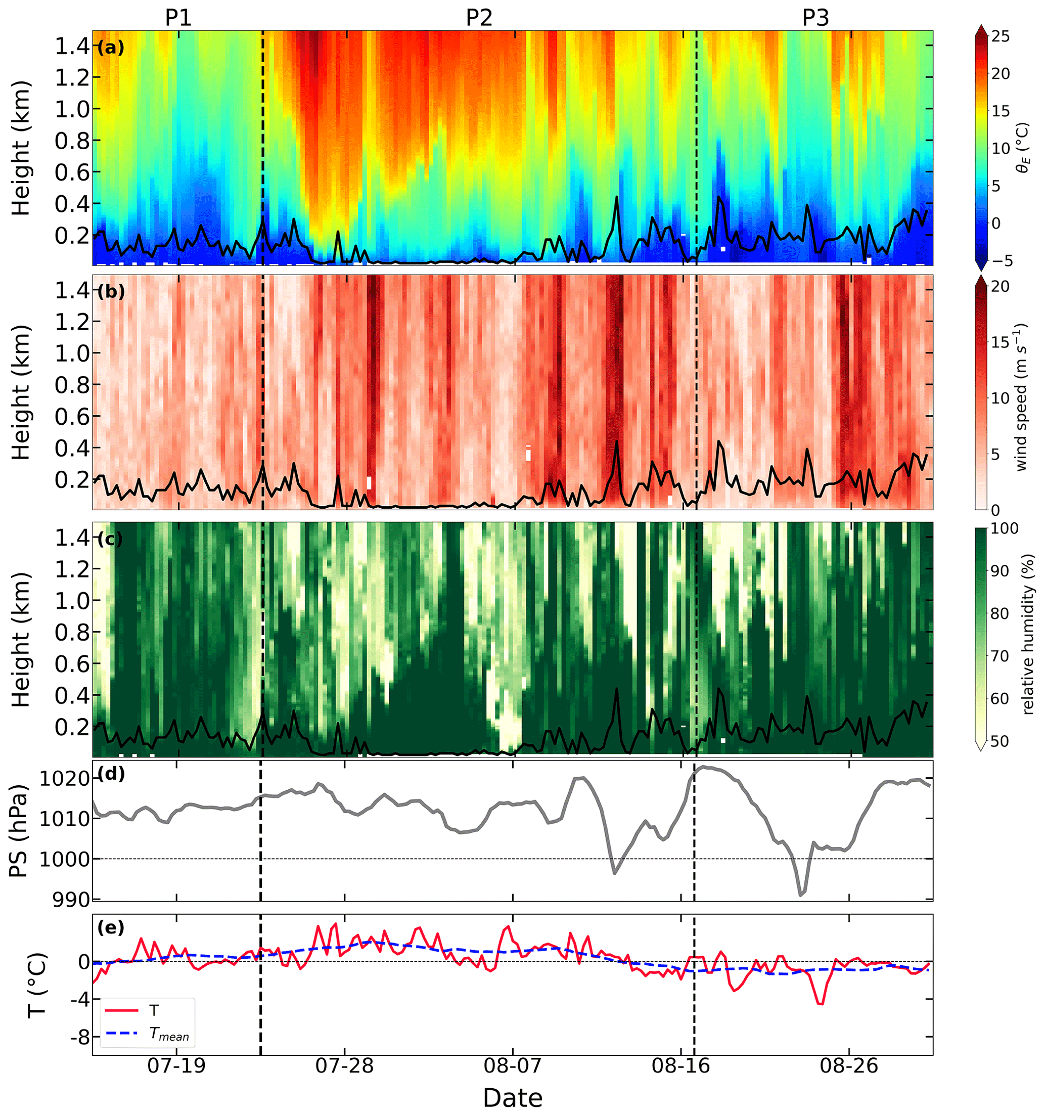
4.4 Case study no. 2: severely suppressed ABL, 15 July–30 August 2020
The Arctic ABL is suppressed most of the time, especially in the late summer for more than a month. We choose the severely suppressed ABL in this period as a case to analyze the influences of the vertical thermal structure and near-surface conditions on the ABLH. The results are shown in Fig. 14, and the whole period is divided into three parts, similar to Fig. 13. In P1, the near-surface air temperature is constrained to ∼ 0 ∘C due to the melting surface, and the temperature inversion and weak wind are dominant throughout the lower troposphere, which suppresses the ABL development. In P2, warm-air advection occurs in the lower troposphere, strengthening the temperature inversion and contributing to further ABL suppression and an ABLH often lower than 100 m. Because of the constrained near-surface temperature, this structure is distinct from that of the spring transition period when warm-air advection facilitates ABL development. In P3, the near-surface and upper-layer temperatures start to decrease and the temperature inversion weakens, which makes the ABLH periodically increase up to ∼ 400 m. Despite that, the ABL is still stably stratified, and the ample moisture and clouds cannot contribute significantly to the ABL development, which is consistent with Shupe et al. (2013). It is important to note that the Polarstern transited from near the sea-ice edge to near the North Pole during the second half of P2; thus, the transition towards weaker temperature inversions is related to both spatial and seasonal shifts. In summary, the suppression of the ABL during the summer melt period results from strong temperature inversions and weak winds, and cloud-driven turbulent mixing is inhibited from interacting with the surface layer due to the near-surface stability. In this period, warm-air advection events enhance the ABL suppression, which is the inverse of the behavior observed during the transition period.
The MOSAiC and SHEBA observations were both made over Arctic sea ice during yearlong periods. In terms of the location of observation sites, the SHEBA campaign took place in the Beaufort and Chukchi seas (Perovich et al., 2003), whereas MOSAiC observations took place along the transpolar drift for much of the year, in the higher latitudes of the Fram Strait in June, July, and early August, and again near the North Pole in late August and September. The comparison between the two campaigns could provide insight into the spatial and temporal variability in the Arctic ABL structure. The monthly ABLHs of the two campaigns are presented in Fig. 15a. The overall distributions of the ABLH are similar during the annual cycle; however, the SHEBA ABLH is significantly higher than the MOSAiC ABLH in June and August. We will discuss these differences based on the ABL thermal structure.
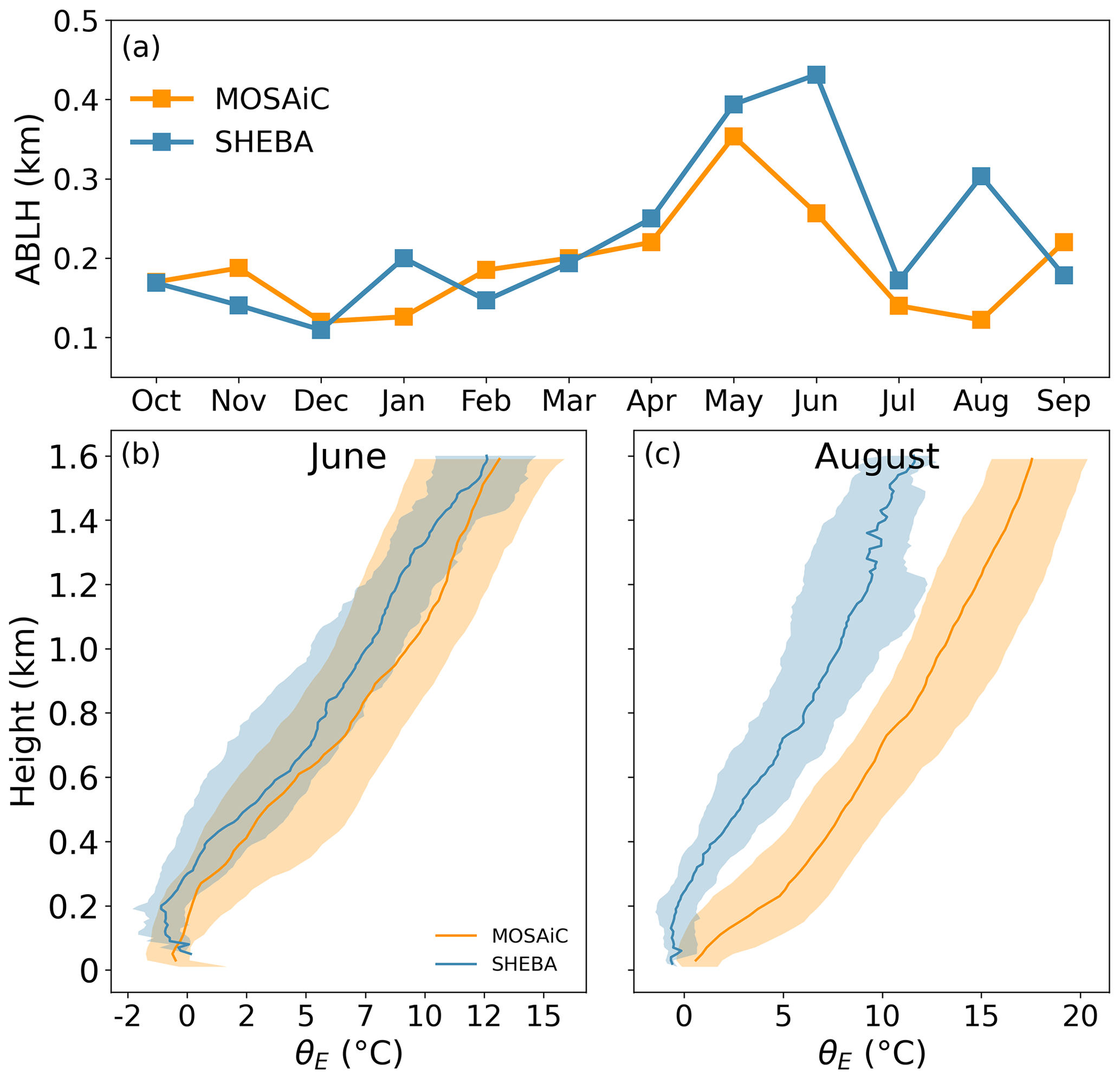
Figure 15Comparison of the ABL during SHEBA (blue squares, lines, and shading) and MOSAiC (yellow squares, lines, and shading), including (a) the annual cycle of the monthly median ABLH and monthly θE profiles in (b) June and (c) August. The solid lines in panels (b) and (c) indicate the median profiles, and the shading indicates the range of 25th and 75th percentile profiles. The median ABLHs of SHEBA are from Dai et al. (2011).
Comparisons of monthly θE profiles between the two campaigns during June and August are presented in Fig. 15b and c. It is clear that θE within the lower troposphere during MOSAiC is much higher than that during SHEBA, especially in August. In June, the near-surface θE values from both campaigns are close, as both were over melting sea ice. However, on average, the upper-layer θE during SHEBA is lower than that during MOSAiC, especially at a height of around 200 m, which results in decreased low-level stability that supports ABL development. This difference explains why the monthly SHEBA ABLH increases from May to June, but the monthly MOSAiC ABLH decreases at this time. For SHEBA, the increased air temperature in the lower troposphere combined with constrained near-surface θE results in a significant temperature inversion in July that suppresses the ABL development (not shown). Thus, the ABLH values for SHEBA and MOSAiC are comparable in July. In August, the θE profiles from the two campaigns are significantly different. The surface at both locations is still mostly constrained to be near the melting point, while the lower troposphere at SHEBA starts to cool more than that at MOSAiC. The SHEBA θE profile exhibits a near-neutral or convective state, while the MOSAiC θE profile shows a further enhanced surface temperature inversion due to warm-air advection aloft, which maintains the ABL suppression. In summary, the increase in air temperature in the lower troposphere in early summer during MOSAiC precedes that during SHEBA, whereas the cooling of the lower troposphere in late summer during MOSAiC lags that during SHEBA. These are the main factors contributing to the ABLH differences between the two campaigns.
The atmospheric warming during the MOSAiC summer may be attributed to ongoing Arctic warming that contributes a different atmospheric structure, but the impacts of transit periods and different synoptic backgrounds should also be considered. First, there is the complexity of the transit periods during MOSAiC. During the first half of June, Polarstern traveled northward into a somewhat loosened sea-ice pack and followed open-water areas as much as possible. If anything, the higher fraction of open water along this transit path would promote more heat exchange between the surface and ABL and a higher ABLH than the regional ice pack (e.g., Fig. 7), which suggests that the observed difference between MOSAiC and SHEBA cannot be explained by this transit period. However, in the first part of August, when Polarstern transited preferentially through open-water areas during its movement further north, the transit environment was in a persistent melting state with warm-air advection aloft. It is not clear how this transit ultimately impacted the monthly ABLH results, although the values during the transit period were lower than those during the final 10 d of August when Polarstern was again passively drifting with the sea ice (Figs. 7, 14). Thus, some of the difference compared with SHEBA at this time could have been attributed to the specific conditions encountered during movement of the vessel. Additionally, these two campaigns were in different storm tracks with markedly different types of regional advection patterns. For example, in summer, MOSAiC was approaching the Fram Strait where northward warm-air advection is common. Thus, synoptic variability likely plays a big role in the ABL thermal structure. In summary, there is large variability in the Arctic ABL structure during summer caused by the surface melting state, and more detailed assessments are needed to study the specific causes of atmospheric warming and the possible influences of changing Arctic conditions on the ABL structure.
This study is carried out using merged radiosounding data and corresponding surface meteorological observations and cloud properties collected during the MOSAiC expedition over a yearlong period. A number of ABLH algorithms are first evaluated, prompting us to implement an improved Ri algorithm that takes cloud effects into consideration. We propose a critical Ri = 0.35 and further analyze its value choice and stability dependence. Subsequently, we use the manually labeled ABLH dataset to study how the atmospheric thermal structure and near-surface conditions impact the characteristics and evolution of the ABL during the MOSAiC year. Lastly, we use two cases to explore the mechanisms of ABL development and suppression over the Arctic sea-ice surface. The main conclusions are outlined in the following.
During the MOSAiC year, the mean ABLH is 231 m, with SBLs, NBLs, and CBLs accounting for 43 %, 31 %, and 26 % of the profiles, respectively. The annual cycle of the Arctic ABLH is clearly characterized by a distinct peak in May and two respective minima in January and July–August. Low-level clouds significantly contribute to the Arctic ABL development during the MOSAiC year, except in winter, when low-level clouds are less frequent. Compared with the SHEBA ABLH, the MOSAiC ABLH is suppressed in June and August, which is caused by increased atmospheric warming in the MOSAiC ABL during the summer melt period compared with SHEBA.
The annual cycle of the ABLH over the Arctic Ocean is primarily controlled by the seasonal evolution of the ABL thermal structure and near-surface meteorological conditions. In the winter period, temperature inversions form due to negative net radiation at the surface and are associated with low ABLHs. In the spring transition period, the rapid increase in the near-surface temperature weakens the temperature inversion, facilitating the development of the ABL. In the summer melt period, temperature inversions result from a fixed surface temperature at the melting point and warm-air advection aloft, which suppresses the ABL development. For near-surface conditions and free-flow stability, a negative θEgrad and large TKE dissipation rate are characteristic of significant ABL development. In addition, empirical formulas relating the ABLH to friction velocity, near-surface, and free-flow stabilities are also tested, and the results suggest that the MOSAiC ABLH can be roughly estimated based on these basic variables.
During MOSAiC, the development of the ABL is irregular and only occurs during intermittent periods. The year is characterized by occasions of abrupt growth of the ABLH and intensive ABLH variation for several days thereafter. These unique features are caused by large-scale synoptic processes (e.g., advection events) that bring heat, moisture, and clouds. It is worth noting that some large-scale events can have the opposite effect on the ABL. For example, warm-air advection can facilitate ABL development in the spring transition period but can cause ABL suppression in the summer melt period, when the constrained near-surface temperature cannot respond to the warmth aloft.
The findings reported here provide new insight into the annual variability and properties of the ABL and ABLH over sea ice in the new Arctic. The ABLH contains information directly related to the thermal structure of the ABL and includes the impacts of weather events and large-scale circulations on the ABL structure. The ABL development supported by cloud processes was captured by the improved Ri algorithm, which is similar to Brooks et al. (2017). However, the representativity of these results must still be established by comparing them to additional observations, and the influences of other variables (e.g., energy budget terms) on the ABLH should also be considered in future research.
The radiosonde data are available from the PANGAEA Data Publisher at https://doi.org/10.1594/PANGAEA.943870 (Maturilli et al., 2022). All value-added products and surface meteorological data are available from the archive of the US Department of Energy Atmospheric Radiation Measurement program. The Planetary Boundary Layer Height Value Added Product is available at https://doi.org/10.5439/1150253 (Riihimaki et al., 2019). The cloud property data are available at https://doi.org/10.5439/1871015 (Shupe, 2022). The MOSAiC surface flux and other meteorological data are available from the Arctic Data Center at https://doi.org/10.18739/A2PV6B83F (Cox et al., 2023). The merged sounding–tower data are available from PANGAEA. The SHEBA-based sounding data are available at https://doi.org/10.5065/D6FQ9V0Z (Moritz, 2017).
SP: formal analysis, investigation, methodology, visualization, writing – original draft, and writing – review and editing. QY: conceptualization, formal analysis, project administration, writing – review and editing, funding acquisition, and supervision. MDS: data curation, formal analysis, validation, resources, and writing – review and editing. XX: methodology, validation, and writing – review and editing. BH: formal analysis, validation, and writing – review and editing. DC: formal analysis, validation, writing – review and editing, and supervision. SD: data curation, validation, and writing – review and editing. CL: data curation, formal analysis, validation, visualization, writing – original draft, and writing – review and editing.
The contact author has declared that none of the authors has any competing interests.
Publisher's note: Copernicus Publications remains neutral with regard to jurisdictional claims in published maps and institutional affiliations.
Data used in this paper were produced as part of the international Multidisciplinary drifting Observatory for the Study of Arctic Climate (MOSAiC) expedition with the tag MOSAiC20192020. We thank everyone involved in the expedition of the research vessel Polarstern during MOSAiC in 2019–2020 (AWI_PS122_00), as listed in Nixdorf et al. (2021). A subset of data was obtained from the Atmospheric Radiation Measurement (ARM) User Facility, a US Department of Energy (DOE) Office of Science user facility managed by the Biological and Environmental Research program. The Alfred Wegener Institute, the DOE ARM program, and the German Weather Service are acknowledged for their contributions to the MOSAiC sounding program.
This study has been supported by the National Natural Science Foundation of China (grant nos. 42105072 and 41941009), the National Key Research and Development Program of China (grant no. 2022YFE0106300), the Guangdong Basic and Applied Basic Research Foundation (grant nos. 2021A1515012209 and 2020B1515020025), the China Postdoctoral Science Foundation (grant no. 2021M693585), and the Norges Forskningsråd (grant no. 328886). MDS was supported by the US National Science Foundation (grant no. OPP-1724551), the DOE Atmospheric System Research program (grant nos. DE-SC0019251 and DE-SC0023036), and the National Oceanic and Atmospheric Administration Global Ocean Monitoring and Observing program (FundRef NA22OAR4320151).
This paper was edited by Thijs Heus and reviewed by two anonymous referees.
Akansu, E. F., Dahlke, S., Siebert, H., and Wendisch, M.: Determining the surface mixing layer height of the Arctic atmospheric boundary layer during polar night in cloudless and cloudy conditions, EGUsphere [preprint], https://doi.org/10.5194/egusphere-2023-629, 2023.
Andreas, E. L., Claffy, K. J., and Makshtas, A. P.: Low-level atmospheric jets and inversions over the western Weddell Sea, Bound.-Lay. Meteorol., 97, 459–486, https://doi.org/10.1023/A:1002793831076, 2000.
Banta, R. M., Pichugina, Y. L., and Newsom, R. K.: Relationship between low-level jet properties and turbulence kinetic energy in the nocturnal stable boundary layer, J. Atmos. Sci., 60, 2549–2555, https://doi.org/10.1175/1520-0469(2003)060<2549:RBLJPA>2.0.CO;2, 2003.
Barten, J. G. M., Ganzeveld, L. N., Steeneveld, G. J., Blomquist, B. W., Angot, H., Archer, S. D., Bariteau, L., Beck, I., Boyer, M., von der Gathen, P., Helmig, D., Howard, D., Hueber, J., Jacobi, H.-W., Jokinen, T., Laurila, T., Posman, K. M., Quéléver, L., Schmale, J., Shupe, M. D., and Krol, M. C.: Low ozone dry deposition rates to sea ice during the MOSAiC field campaign: Implications for the Arctic boundary layer ozone budget, Elementa: Sci. Anthrop., 11, 00086, https://doi.org/10.1525/elementa.2022.00086, 2023.
Basu, S., Holtslag, A. A. M., van de Wiel, B. J. H., Moene, A. F., and Steeneveld, G. J.: An inconvenient “truth” about using sensible heat flux as a surface boundary condition in models under stably stratified regimes, Acta Geophys., 56, 88–99, https://doi.org/10.2478/s11600-007-0038-y, 2008.
Basu, S., Holtslag, A. A. M., Caporaso, L., Riccio, A., and Steeneveld, G. J.: Observational Support for the Stability Dependence of the Bulk Richardson Number Across the Stable Boundary Layer, Bound.-Lay. Meteorol., 150, 515–523, https://doi.org/10.1007/s10546-013-9878-y, 2014.
Blunden, J. and Arndt, D. S.: A Look at 2018: Takeaway Points from the State of the Climate Supplement, B. Am. Meteorol. Soc., 100, 1625–1636, https://doi.org/10.1175/bams-d-19-0193.1, 2019.
Brooks, I. M., Tjernström, M., Persson, P. O. G., Shupe, M. D., Atkinson, R. A., Canut, G., Birch, C. E., Mauritsen, T., Sedlar, J., and Brooks, B. J.: The Turbulent Structure of the Arctic Summer Boundary Layer During The Arctic Summer Cloud-Ocean Study, J. Geophys. Res.-Atmos., 122, 9685–9704, https://doi.org/10.1002/2017jd027234, 2017.
Busch, N., Ebel, U., Kraus, H., and Schaller, E.: The structure of the subpolar inversion-capped ABL, Arch. Meteor. Geophy. A, 31, 1–18, https://doi.org/10.1007/BF02257738, 1982.
Cox, C., Gallagher, M., Shupe, M., Persson, O., Blomquist, B., Grachev, A., Riihimaki, L., Kutchenreiter, M., Morris, V., Solomon, A., Brooks, I., Costa, D., Gottas, D., Hutchings, J., Osborn, J., Morris, S., Preusser, A., Uttal, T.: Met City meteorological and surface flux measurements (Level 3 Final), Multidisciplinary drifting Observatory for the Study of Arctic Climate (MOSAiC), central Artic, October 2019–September 2020, Arctic Data Center [data set], https://doi.org/10.18739/A2PV6B83F, 2023.
Dahlke, S., Shupe, M. D., Cox, C., Brooks, I. M., Blomquist, B., and Persson, P. O. G.: Extended radiosonde profiles 2019/09–2020/10 during MOSAiC Legs PS122/1–PS122/5, PANGAEA [data set], submitted, 2023.
Dai, C., Gao, Z., Wang, Q., and Cheng, G.: Analysis of Atmospheric Boundary Layer Height Characteristics over the Arctic Ocean Using the Aircraft and GPS Soundings, Atmospheric Ocean. Sci., 4, 124–130, https://doi.org/10.1080/16742834.2011.11446916, 2011.
Davy, R. and Esau, I.: Differences in the efficacy of climate forcings explained by variations in atmospheric boundary layer depth, Nat. Commun., 7, 11690, https://doi.org/10.1175/BAMS-D-11-00187.1, 2016.
Esau, I., Pettersson, L. H., Cancet, M., Chapron, B., Chernokulsky, A., Donlon, C., Sizov, O., Soromotin, A., and Johannesen, J. A.: The Arctic Amplification and Its Impact: A Synthesis through Satellite Observations, Remote Sens.-Basel, 15, 1354, https://doi.org/10.3390/rs15051354, 2023.
Francis, J. A. and Hunter, E.: New insight into the disappearing Arctic sea ice, Eos T. Am. Geophys. Un., 87, 509–511, https://doi.org/10.1029/2006EO460001, 2006.
Graversen, R. G., Mauritsen, T., Tjernström, M., Kallen, E., and Svensson, G.: Vertical structure of recent Arctic warming, Nature, 451, 53–56, https://doi.org/10.1038/nature06502, 2008.
Heffter, J. L.: Transport layer depth calculations, Second Joint Conference on Applications of Air Pollution Meteorology, New Orleans, La., United States, 24–27 March 1980, 781–787, https://doi.org/10.1175/1520-0477-61.1.65, 1980.
Holtslag, A. A. M., Svensson, G., Baas, P., Basu, S., Beare, B., Beljaars, A. C. M., Bosveld, F. C., Cuxart, J., Lindvall, J., Steeneveld, G. J., Tjernström, M., and Van De Wiel, B. J. H.: Stable atmospheric boundary layers and diurnal cycles: Challenges for weather and climate models, B. Am. Meteorol. Soc., 94, 1691–1706, https://doi.org/10.1038/ncomms11690, 2013.
Jozef, G., Cassano, J., Dahlke, S., and de Boer, G.: Testing the efficacy of atmospheric boundary layer height detection algorithms using uncrewed aircraft system data from MOSAiC, Atmos. Meas. Tech., 15, 4001–4022, https://doi.org/10.5194/amt-15-4001-2022, 2022.
Jozef, G. C., Cassano, J. J., Dahlke, S., Dice, M., Cox, C. J., and de Boer, G.: An Overview of the Vertical Structure of the Atmospheric Boundary Layer in the Central Arctic during MOSAiC, EGUsphere [preprint], https://doi.org/10.5194/egusphere-2023-780, 2023.
Kim, J. and Mahrt, L.: Simple Formulation of Turbulent Mixing in the Stable Free Atmosphere and Nocturnal Boundary Layer, Tellus, 44A, 381–39, https://doi.org/10.3402/tellusa.v44i5.14969, 1992.
Kljun, N., Calanca, P., Rotach, M. W., and Schmid, H. P.: A simple two-dimensional parameterisation for Flux Footprint Prediction (FFP), Geosci. Model Dev., 8, 3695–3713, https://doi.org/10.5194/gmd-8-3695-2015, 2015.
Knudsen, E. M., Heinold, B., Dahlke, S., Bozem, H., Crewell, S., Gorodetskaya, I. V., Heygster, G., Kunkel, D., Maturilli, M., Mech, M., Viceto, C., Rinke, A., Schmithüsen, H., Ehrlich, A., Macke, A., Lüpkes, C., and Wendisch, M.: Meteorological conditions during the ACLOUD/PASCAL field campaign near Svalbard in early summer 2017, Atmos. Chem. Phys., 18, 17995–18022, https://doi.org/10.5194/acp-18-17995-2018, 2018.
Knust, R.: Polar Research and Supply Vessel POLARSTERN operated by the Alfred-Wegener-Institute, Journal of Large-scale Research Facilities JLSRF, 3, 119, https://doi.org/10.17815/jlsrf-3-163, 2017.
Konor, C. S., Boezio, G. C., Mechoso, C. R., and Arakawa, A.: Parameterization of PBL Processes in an Atmospheric General Circulation Model: Description and Preliminary Assessment, Mon. Weather Rev., 137, 1061–1082, https://doi.org/10.1175/2008mwr2464.1, 2009.
Landrum, L. and Holland, M. M.: Extremes become routine in an emerging new Arctic, Nat. Clim. Change, 10, 1108–1115, https://doi.org/10.1038/s41558-020-0892-z, 2020.
Lenschow D. H., Zhou M., Zeng X., Chen L., and Xu X.: Measurements of fine-scale structure at the top of marine stratocumulus, Bound.-Lay. Meteorol., 97, 331–357, https://doi.org/10.1023/A:1002780019748, 2000.
Liu, S. and Liang, X.: Observed Diurnal Cycle Climatology of Planetary Boundary Layer Height, J. Climate, 23, 5790–5809, https://doi.org/10.1175/2010jcli3552.1, 2010.
Mahrt, L.: Modelling the depth of the stable boundary-layer, Bound.-Lay. Meteorol., 21, 3–19, https://doi.org/10.1007/BF00119363, 1981.
Mahrt, L.: Stably stratified atmospheric boundary layers, Annu. Rev. Fluid Mech., 46, 23–45, https://doi.org/10.1146/annurev-fluid-010313-141354, 2014.
Mahrt L., Heald R. C., Lenschow D. H., Stankov B. B., and Troen I. B.: An observational study of the structure of the nocturnal boundary layer, Bound.-Lay. Meteorol., 17, 247–264, https://doi.org/10.1007/BF00117983, 1979.
Marsik, F. J., Fischer, K. W., McDonald, T. D., and Samson, P. J.: Comparison of Methods for Estimating Mixing Height Used during the 1992 Atlanta Field Intensive, J. Appl. Meteorol. Clim., 34, 1802–1814, https://doi.org/10.1175/1520-0450(1995)034<1802:Comfem>2.0.Co;2, 1995.
Martucci, G., Matthey, R., and Mitev, V.: Comparison between backscatter lidar and radiosonde measurements of the diurnal and nocturnal stratification in the lower troposphere, J. Atmos. Ocean. Tech., 24, 1231–1244, https://doi.org/10.1175/JTECH2036.1, 2007.
Maturilli, M., Sommer, M., Holdridge, D. J., Dahlke, S., Graeser, J., Sommerfeld, A., Jaiser, R., Deckelmann, H., and Schulz, A.: MOSAiC radiosonde data (level 3) [data set], PANGAEA, https://doi.org/10.1594/PANGAEA.943870, 2022.
Matveeva, T. A. and Semenov, V. A.: Regional Features of the Arctic Sea Ice Area Changes in 2000–2019 versus 1979–1999 Periods, Atmosphere, 13, 1434, https://doi.org/10.3390/atmos13091434, 2022.
Meier, W. N., and Stroeve, J.: An updated assessment of the changing Arctic sea ice cover, Oceanography, 35, 10–19, https://doi.org/10.5670/oceanog.2022.114, 2022.
Moritz, R.: Soundings, Ice Camp NCAR/GLAS raobs. (ASCII). Version 2.0., University of Washington, UCAR/NCAR – Earth Observing Laboratory [data set], https://doi.org/10.5065/D6FQ9V0Z, 2017.
Nixdorf, U., Dethloff, K., Rex, M., Shupe, M., Sommerfeld, A., Perovich, D. K., Nicolaus, M., Heuze, C., Rabe, B., Loose, B., Damm, E., Gradinger, R., Fong, A., Maslowski, W., Rinke, A., Kwok, R., Spreen, G., Wendisch, M., Herber, A., Hirsekorn, M., Mohaupt, V., Frickenhaus, S., Immerz, A., Weiss-Tuider, K., Koenig, B., Mengedoht, D., Regnery, J., Gerchow, P., Ransby, D., Krumpen, T., Morgenstern, A., Haas, C., Kanzow, T., Rack, F., Saitzev, V., Sokolov, V., Makarov, A., Schwarze, S., Wunderlick, T., Wurr, K., Boetius, A.: MOSAiC extended acknowledgement, Zenodo, https://doi.org/10.5281/zenodo.5541624, 2021.
Overland, J. E. and Davidson, K. L.: Geostrophic drag coefficients over sea ice, Tellus A, 44, 54–66, https://doi.org/10.3402/tellusa.v44i1.17118, 1992.
Overland, J. E., Dunlea, E. J., Box, J. E., Corell, R. W., Forsius, M., Kattsov, V. M., Olsen, M. S., Pawlak, J., Reiersen, L. O., and Wang, M.: The urgency of Arctic change, Polar Sci., 21, 6–13, https://doi.org/10.1016/j.polar.2018.11.008, 2019.
Palo, T., Vihma, T., Jaagus, J., and Jakobson, E.: Observations of temperature inversions over central Arctic sea ice in summer, Q. J. Roy. Meteor. Soc., 143, 2741–2754, https://doi.org/10.1002/qj.3123, 2017.
Perovich, D. K., Grenfell, T. C., Richter-Menge, J. A., Light, B., Tucker III, W. B., and Eicken, H.: Thin and thinner: Sea ice mass balance measurements during SHEBA, J. Geophys. Res.-Oceans, 108, 8050, https://doi.org/10.1029/2001JC001079, 2003.
Persson, P. O. G., Fairall, C. W., Andreas, E. L., Guest, P. S., and Perovich, D. K.: Measurements near the Atmospheric Surface Flux Group tower at SHEBA: Near-surface conditions and surface energy budget, J. Geophys. Res.-Oceans, 107, 35, https://doi.org/10.1029/2000jc000705, 2002.
Pollard R. T., Rhines P. B., and Thompson R.: The deepening of the wind-mixed layer, Geophys. Fluid Dyn., 3, 381–404, https://doi.org/10.1080/03091927208236105, 1973.
Richardson, H., Basu, S., and Holtslag, A. A. M.: Improving Stable Boundary-Layer Height Estimation Using a Stability-Dependent Critical Bulk Richardson Number, Bound.-Lay. Meteorol., 148, 93–109, https://doi.org/10.1007/s10546-013-9812-3, 2013.
Riihimaki, L., Sivaraman, C., and Zhang, D.: Planetary Boundary Layer Height (PBLHTSONDE1MCFARL), Atmospheric Radiation Measurement (ARM) User Facility, ARM Data Center [data set], https://doi.org/10.5439/1150253, 2019.
Seibert, P., Beyrich, F., Gryning, S. E., Joffre, S., Rasmussen, A., and Tercier, P.: Review and intercomparison of operational methods for the determination of the mixing height, Atmos. Environ., 34, 1001–1027, https://doi.org/10.1016/s1352-2310(99)00349-0, 2000.
Seidel, D. J., Ao, C. O., and Li, K.: Estimating climatological planetary boundary layer heights from radiosonde observations: Comparison of methods and uncertainty analysis, J. Geophys. Res.-Atmos., 115, D16113, https://doi.org/10.1029/2009JD013680, 2010.
Seidel, D. J., Zhang, Y. H., Beljaars, A., Golaz, J. C., Jacobson, A. R., and Medeiros, B.: Climatology of the planetary boundary layer over the continental United States and Europe, J. Geophys. Res.-Atmos., 117, 15, https://doi.org/10.1029/2012jd018143, 2012.
Shupe, M. D.: ShupeTurner cloud microphysics product, ARM Mobile Facility (MOS) MOSAiC (Drifting Obs – Study of Arctic Climate), ARM Data Center [data set], https://doi.org/10.5439/1871015, 2022.
Shupe, M. D., and Intrieri, J. M.: Cloud radiative forcing of the Arctic surface: The influence of cloud properties, surface albedo, and solar zenith angle, J. Climate, 17, 616–628, https://doi.org/10.1175/1520-0442(2004)017<0616:CRFOTA>2.0.CO;2, 2004.
Shupe, M. D., Walden, V. P., Eloranta, E., Uttal, T., Campbell, J. R., Starkweather, S. M., and Shiobara, M.: Clouds at Arctic Atmospheric Observatories. Part I: Occurrence and Macrophysical Properties, J. Appl. Meteorol. Clim., 50, 626–644, https://doi.org/10.1175/2010JAMC2467.1, 2011.
Shupe, M. D., Persson, P. O. G., Brooks, I. M., Tjernström, M., Sedlar, J., Mauritsen, T., Sjogren, S., and Leck, C.: Cloud and boundary layer interactions over the Arctic sea ice in late summer, Atmos. Chem. Phys., 13, 9379–9399, https://doi.org/10.5194/acp-13-9379-2013, 2013.
Shupe, M. D., Turner, D. D., Zwink, A., Theiman, M. M., Mlawer, M. J., and Shippert T. R.: Deriving Arctic cloud microphysics at Barrow: Algorithms, results, and radiative closure, J. Appl. Meteorol. Clim., 54, 1675–1689, https://doi.org/10.1175/JAMC-D-15-0054.1, 2015.
Shupe, M. D., Rex, M., Blomquist, B., Persson, P. O. G., Schmale, J., Uttal, T., Althausen, D., Angot, H., Archer, S., Bariteau, L., Beck, I., Bilberry, J., Bucci, S., Buck, C., Boyer, M., Brasseur, Z., Brooks, I. M., Calmer, R., Cassano, J., Castro, V., Chu, D., Costa, D., Cox, C. J., Creamean, J., Crewell, S., Dahlke, S., Damm, E., de Boer, G., Deckelmann, H., Dethloff, K., Dütsch, M., Ebell, K., Ehrlich, A., Ellis, J., Engelmann, R., Fong, A. A., Frey, M. M., Gallagher, M. R., Ganzeveld, L., Gradinger, R., Graeser, J., Greenamyer, V., Griesche, H., Griffiths, S., Hamilton, J., Heinemann, G., Helmig, D., Herber, A., Heuzé, C., Hofer, J., Houchens, T., Howard, D., Inoue, J., Jacobi, H.-W., Jaiser, R., Jokinen, T., Jourdan, O., Jozef, G., King, W., Kirchgaessner, A., Klingebiel, M., Krassovski, M., Krumpen, T., Lampert, A., Landing, W., Laurila, T., Lawrence, D., Lonardi, M., Loose, B., Lüpkes, C., Maahn, M., Macke, A., Maslowski, W., Marsay, C., Maturilli, M., Mech, M., Morris, S., Moser, M., Nicolaus, M., Ortega, P., Osborn, J., Pätzold, F., Perovich, D. K., Petäjä, T., Pilz, C., Pirazzini, R., Posman, K., Powers, H., Pratt, K. A., Preußer, A., Quéléver, L., Radenz, M., Rabe, B., Rinke, A., Sachs, T., Schulz, A., Siebert, H., Silva, T., Solomon, A., Sommerfeld, A., Spreen, G., Stephens, M., Stohl, A., Svensson, G., Uin, J., Viegas, J., Voigt, C., von der Gathen, P., Wehner, B., Welker, J. M., Wendisch, M., Werner, M., Xie, Z., and Yue, F.: Overview of the MOSAiC expedition – Atmosphere, Elementa: Sci. Anthrop., 10, 00060, https://doi.org/10.1525/elementa.2021.00060, 2022.
Silber, I. and Shupe, M. D.: Insights on sources and formation mechanisms of liquid-bearing clouds over MOSAiC examined from a Lagrangian framework, Elementa: Sci. Anthrop., 10, 000071, https://doi.org/10.1525/elementa.2021.000071, 2022.
Sivaraman, C., McFarlane, S., Chapman, E., Jensen, M., Toto, T., Liu, S., and Fischer, M.: Planetary Boundary Layer Height (PBL) Value Added Product (VAP): Radiosonde Retrievals, University of Maryland, United States, DOE/SC-ARM/TR-132, https://doi.org/10.2172/1808688, 2013.
Snyder, B. J. and Strawbridge, K. B.: Meteorological analysis of the Pacific 2001 air quality field study, Atmos. Environ., 38, 5733–5743, https://doi.org/10.1016/j.atmosenv.2004.02.068, 2004.
Solomon, A., Shupe, M. D., Persson, P. O. G., and Morrison, H.: Moisture and dynamical interactions maintaining decoupled Arctic mixed-phase stratocumulus in the presence of a humidity inversion, Atmos. Chem. Phys., 11, 10127–10148, https://doi.org/10.5194/acp-11-10127-2011, 2011.
Sørensen, J. H., Rasmussen, A., Ellermann, T., and Lyck, E.: Mesoscale influence on long-range transport – evidence from ETEX modelling and observations, Atmos. Environ., 32, 4207–4217, https://doi.org/10.1016/S1352-2310(98)00183-6, 1998.
Sotiropoulou, G., Sedlar, J., Tjernström, M., Shupe, M. D., Brooks, I. M., and Persson, P. O. G.: The thermodynamic structure of summer Arctic stratocumulus and the dynamic coupling to the surface, Atmos. Chem. Phys., 14, 12573–12592, https://doi.org/10.5194/acp-14-12573-2014, 2014.
Steeneveld, G. J., van de Wiel, B. J. H., and Holtslag, A. A. M.: Comments on deriving the equilibrium height of the stable boundary layer, Q. J. Roy. Meteor. Soc., 133, 261–264, https://doi.org/10.1002/qj.26, 2007a.
Steeneveld, G. J., van de Wiel, B. J. H., and Holtslag, A. A. M.: Diagnostic Equations for the Stable Boundary Layer Height: Evaluation and Dimensional Analysis, J. Appl. Meteorol. Clim., 46, 212–225, https://doi.org/10.1175/JAM2454.1, 2007b.
Sterk, H. A. M., Steeneveld G. J., and Holtslag A. A. M.: The role of snow-surface coupling, radiation, and turbulent mixing in modeling a stable boundary layer over Arctic sea ice, J. Geophys. Res.-Atmos., 118, 1199–1217, https://doi.org/10.1002/jgrd.50158, 2014.
Tjernström, M. and Graversen, R. G.: The vertical structure of the lower Arctic troposphere analysed from observations and the ERA-40 reanalysis, Q. J. Roy. Meteor. Soc., 135, 431–443, https://doi.org/10.1002/qj.380, 2009.
Tjernström, M., Balsley, B. B., Svensson, G., and Nappo, C. J.: The Effects of Critical Layers on Residual Layer Turbulence, J. Atmos. Sci., 66, 468–480, https://doi.org/10.1175/2008jas2729.1, 2009.
Tjernström, M., Birch, C. E., Brooks, I. M., Shupe, M. D., Persson, P. O. G., Sedlar, J., Mauritsen, T., Leck, C., Paatero, J., Szczodrak, M., and Wheeler, C. R.: Meteorological conditions in the central Arctic summer during the Arctic Summer Cloud Ocean Study (ASCOS), Atmos. Chem. Phys., 12, 6863–6889, https://doi.org/10.5194/acp-12-6863-2012, 2012.
Uttal, T., Curry, J. A., McPhee, M. G., Perovich, D. K., Moritz, R. E., Maslanik, J. A., Guest, P. S., Stern, H. L., Moore, J. A., Turenne, R., Heiberg, A., Serreze, M. C., Wylie, D. P., Persson, O. G., Paulson, C. A., Halle, C., Morison, J. H., Wheeler, P. A., Makshtas, A., Welch, H., Shupe, M. D., Intrieri, J. M., Stamnes, K., Lindsey, R. W., Pinkel, R., Pegau, W. S., Stanton, T. P., and Grenfeld, T. C.: Surface Heat Budget of the Arctic Ocean, B. Am. Meteorol. Soc., 83, 255–276, https://doi.org/10.1175/1520-0477(2002)083<0255:Shbota>2.3.Co;2, 2002.
Vihma, T.: Effects of Arctic Sea Ice Decline on Weather and Climate: A Review, Surv. Geophys., 35, 1175–1214, https://doi.org/10.1007/s10712-014-9284-0, 2014.
Vihma, T., Kilpelainen, T., Manninen, M., Sjoblom, A., Jakobson, E., Palo, T., Jaagus, J., and Maturilli, M.: Characteristics of Temperature and Humidity Inversions and Low-Level Jets over Svalbard Fjords in Spring, Adv. Meteorol., 2011, 14, https://doi.org/10.1155/2011/486807, 2011.
Vogelezang, D. H. P. and Holtslag, A. A. M.: Evaluation and model impacts of alternative boundary-layer height formulations, Bound.-Lay. Meteorol., 81, 245–269, https://doi.org/10.1007/BF02430331, 1996.
Vüllers, J., Achtert, P., Brooks, I. M., Tjernström, M., Prytherch, J., Burzik, A., and Neely III, R.: Meteorological and cloud conditions during the Arctic Ocean 2018 expedition, Atmos. Chem. Phys., 21, 289–314, https://doi.org/10.5194/acp-21-289-2021, 2021.
Wang, S., Wang, Q., Jordan, R. E., and Persson, P. O. G.: Interactions among longwave radiation of clouds, turbulence, and snow surface temperature in the Arctic: A model sensitivity study, J. Geophys. Res.-Atmos., 106, 15323–15333, https://doi.org/10.1029/2000JD900358, 2001.
Wetzel, C. and Bruemmer, B.: An Arctic inversion climatology based on the European Centre Reanalysis ERA-40, Meteorol. Z, 20, 589–600, https://doi.org/10.1127/0941-2948/2011/0295, 2011.
Zhang, Y., Gao, Z., Li, D., Li, Y., Zhang, N., Zhao, X., and Chen, J.: On the computation of planetary boundary-layer height using the bulk Richardson number method, Geosci. Model Dev., 7, 2599–2611, https://doi.org/10.5194/gmd-7-2599-2014, 2014.
Zhang, Y. J., Sun, K., Gao, Z. Q., Pan, Z. T., Shook, M. A., and Li, D.: Diurnal Climatology of Planetary Boundary Layer Height Over the Contiguous United States Derived From AMDAR and Reanalysis Data, J. Geophys. Res.-Atmos., 125, e2020JD032803, https://doi.org/10.1029/2020JD032803, 2020.
Zilitinkevich, S. S.: On the determination of the height of the Ekman boundary layer, Bound.-Lay. Meteorol., 3, 141–145, https://doi.org/10.1007/BF02033914, 1972.
Zilitinkevich, S. S.: Third-order transport due to internal waves and non-local turbulence in the stably stratified surface layer, Q. J. Roy. Meteor. Soc., 128, 913–925, https://doi.org/10.1256/0035900021643746, 2002.
Zilitinkevich, S. S.: The height of the atmospheric planetary boundary layer: State of the art and new development, in: National Security and Human Health Implications of Climate Change (NATO Science for Peace and Security Series C: Environmental Security), edited by: Fernando, H. J. S., Klaić, Z., and McCulley, J., Springer, Dordrecht, 147–161, https://doi.org/10.1007/978-94-007-2430-3_13, 2012.
Zilitinkevich, S. S. and Baklanov, A.: Calculation Of The Height Of The Stable Boundary Layer In Practical Applications, Bound.-Lay. Meteorol., 105, 389–409, https://doi.org/10.1023/A:1020376832738, 2002.
Zilitinkevich, S. S. and Esau, I. N.: On Integral Measures Of The Neutral Barotropic Planetary Boundary Layer, Bound.-Lay. Meteorol., 104, 371–379. https://doi.org/10.1023/A:1016540808958, 2002.
Zilitinkevich, S. S. and Esau I. N.: The effect of baroclinicity on the depth of neutral and stable planetary boundary layers, Q. J. Roy. Meteor. Soc., 129, 3339–3356, https://doi.org/10.1256/qj.02.94, 2003.
Zilitinkevich, S. S., Elperin, T., Kleeorin, N., and Rogachevskii, I.: Energy- and flux-budget (EFB) turbulence closure model for stably stratified flows. Part I: steady-state, homogeneous regimes. Bound.-Lay. Meteorol., 125, 167–191, https://doi.org/10.1007/s10546-007-9189-2, 2007.
- Abstract
- Introduction
- Measurements
- ABLH determination method and algorithm evaluation
- MOSAiC ABLH variation and controlling factors
- MOSAiC–SHEBA comparison
- Conclusions
- Data availability
- Author contributions
- Competing interests
- Disclaimer
- Acknowledgements
- Financial support
- Review statement
- References