the Creative Commons Attribution 4.0 License.
the Creative Commons Attribution 4.0 License.
 | 21 Jul 2023
Examining cloud vertical structure and radiative effects from satellite retrievals and evaluation of CMIP6 scenarios
Johannes Quaas
Yong Han
Clouds exhibit a wide range of vertical morphologies that are regulated by distinct atmospheric dynamics and thermodynamics and are related to a diversity of microphysical properties and radiative effects. In this study, the new CERES-CloudSat-CALIPSO-MODIS (CCCM) RelD1 dataset is used to investigate the morphology and spatial distribution of different cloud vertical structure (CVS) types during 2007–2010. The combined active and passive satellites provide a more precise CVS than those only based on passive imagers or microwave radiometers. We group the clouds into 12 CVS classes based on how they are located or overlapping in three standard atmospheric layers with pressure thresholds of 440 and 680 hPa. For each of the 12 CVS types, the global average cloud radiative effects (CREs) at the top of the atmosphere, within the atmosphere and at the surface, as well as the cloud heating rate (CHR) profiles are examined. The observations are subsequently used to evaluate the variations in total, high-, middle- and low-level cloud fractions in CMIP6 models. The “historical” experiment during 1850–2014 and two scenarios (ssp245 and ssp585) during 2015–2100 are analyzed. The observational results show a substantial difference in the spatial pattern among different CVS types, with the greatest contrast between high and low clouds. Single-layer cloud fraction is almost 4 times larger on average than multi-layer cloud fraction, with significant geographic differences associated with clearly distinguishable regimes, showing that overlapping clouds are regionally confined. The global average CREs reveal that four types of CVSs warm the planet, while eight of them cool it. The longwave component drives the net CHR profile, and the CHR profiles of multi-layer clouds are more curved and intricate than those of single-layer clouds, resulting in complex thermal stratifications. According to the long-term analysis from CMIP6, the projected total cloud fraction decreases faster over land than over the ocean. The high clouds over the ocean increase significantly, but other types of clouds over land and the ocean continue to decrease, helping to offset the decrease in oceanic total cloud fraction. Moreover, it is concluded that the spatial pattern of CVS types may not be significantly altered by climate change, and only the cloud fraction is influenced. Our findings suggest that long-term observed CVS should be emphasized in the future to better understand CVS responses to anthropogenic forcing and climate change.
- Article
(12368 KB) - Full-text XML
-
Supplement
(6931 KB) - BibTeX
- EndNote


Clouds, as primary regulators of Earth's climate system, have a considerable impact on the radiative budget, the hydrological cycle and the global circulation (Hartmann et al., 1992; Stephens, 2005; Norris et al., 2016). Cloud cover is composed of numerous cloud types that are governed by distinctive atmospheric motions and are associated with various microphysical properties and radiative effects (Chen et al., 2000; Oreopoulos et al., 2017; Wang et al., 2023). Small changes in cloud properties have the potential to either mitigate or amplify the warming effects of greenhouse gases, causing clouds to be one of the most significant sources of uncertainty in climate change research (Slingo, 1990; Garrett and Zhao, 2006).
The overall impact of clouds on the radiative budget is difficult to quantitatively estimate, since it comprises two opposing effects (cooling and warming) depending on the cloud types (Ramanathan et al., 1989). In general, low, highly reflective clouds cool the surface by reflecting the solar radiation, while high, semi-transparent clouds warm it by enabling shortwave radiation to pass through but blocking longwave radiation (Slingo, 1990; Lohmann and Roeckner, 1995). The approximately balanced cloud albedo and greenhouse effect prevent deep convective clouds from either warming or cooling the Earth system (Hartmann and Berry, 2017). However, complex multi-layered clouds have uncertain impacts on the radiative budget due to the coexistence of incompatible magnitudes of warming and cooling effects (Li et al., 2011; Matus and L'ecuyer, 2017). While the global-scale horizontal distributions of the total cloud fraction have been investigated well from multiple sources of datasets (Rossow et al., 1993; King et al., 2013; Vignesh et al., 2020), the spatial distributions of the vertically detailed cloud categories have received less attention. Therefore, it is crucial to accurately measure and quantify the cloud vertical structure (CVS) and its radiative effects.
In addition, evidence suggests that CVS is influenced by global warming. The expectation, based on passive satellites and model simulations, is that the high-cloud fraction would increase, while the low-cloud fraction decreases with a warming climate (Norris et al., 2016). Changes in CVS primarily alter three aspects of cloud properties, i.e., altitude, fraction and composition (liquid or ice), thereby affecting the Earth system energy budget (e.g., Zelinka et al., 2013). Less low-level clouds will mainly reduce albedo effects, while more high-level clouds will mostly enhance greenhouse effects, both of which result in warming (Gettelman and Sherwood, 2016). In contrast, the transition from fewer, larger ice crystals to smaller but plentiful liquid droplets in high latitudes will increase albedo effects and produce a cooling effect (Senior and Mitchell, 1993; Choi et al., 2014; Ceppi et al., 2016), as will the increase in adiabatic cloud water content (Betts and Harshvardhan, 1987). Consequently, an improved understanding of how CVS responds to warming is critical for the study of cloud feedback.
Numerous studies have focused on the CVS obtained from ground-based remote sensors and radiosonde measurements (Dong et al., 2000; Zhang et al., 2019; Luo et al., 2023), but such studies are limited in investigating spatial distributions. Additionally, it has been demonstrated that satellite observations are an essential approach to retrieving the CVS on a global scale. Although many efforts have been made to obtain the CVS based on passive instruments, e.g., in the International Satellite Cloud Climatology Project (ISCCP) and the Moderate Resolution Imaging Spectroradiometer (MODIS) (Rossow and Schiffer, 1999; Chang and Li, 2005; Marchand et al., 2010), these passive satellites have limitations and uncertainties in retrieving overlapped clouds. In contrast, active satellite sensors, such as cloud-profiling radar (CPR) on board CloudSat and the Cloud–Aerosol Lidar with Orthogonal Polarization (CALIOP) on board the Cloud–Aerosol Lidar and Infrared Pathfinder Satellite Observation (CALIPSO), complement and provide detailed insights into CVSs that are elusive when relying solely on passive imagers and microwave radiometers (Stubenrauch et al., 2010; Li et al., 2015; Oreopoulos et al., 2017). However, to date, there are only a few products available that provide global cloud radiative effect (CRE) based on active satellite sensors, posing a challenge to the investigation of the CRE of various cloud types. The Clouds and the Earth's Radiant Energy System (CERES) instrument retrieves shortwave and longwave broadband radiation at the top of the atmosphere (TOA) (Wielicki et al., 1996). Unlike TOA irradiance observations, estimating the surface or atmosphere radiation budget requires radiative transfer computations with adequate model inputs of cloud properties (Smith et al., 2004). There are currently two kinds of mainstream products that provide the cloud vertical profiles and the computed CRE simultaneously. One is from the CloudSat Data Processing Center; it offers the cloud vertical boundaries merged from CPR and CALIOP in the Level-2B GEOPROF-LIDAR product as well as irradiance profiles computed by CPR, CALIOP and MODIS in the Level-2B FLXHR-LIDAR product (L'ecuyer et al., 2008; Henderson et al., 2013; Mace and Zhang, 2014). The other is from NASA's Langley Research Center; it produces the A-Train Integrated CERES-CALIPSO-CloudSat-MODIS (CCCM) product (Kato et al., 2011, 2021). Both the Level-2B FLXHR-LIDAR and the CCCM products demonstrate higher agreement with CERES TOA observations than the irradiances estimated using only MODIS-derived cloud properties (Ham et al., 2017, 2022). These advancements are achieved by the improvement of detecting vertically resolved cloud structures and multi-layered clouds by the active sensors. Therefore, using a combination of active and passive satellite sensors to capture the CVS and CRE is preferable to relying on one single sensor.
In order to better constrain the role of clouds in global climate change, it is necessary in addition to understand long-term variations and trends in CVS, which reflect the changing contributions of CREs to the climate system. Anthropogenic forcing, such as greenhouse gases and aerosols, may have an impact on the cloud fraction and its vertical distributions (Penner et al., 2009; Gryspeerdt et al., 2016). In addition, clouds also respond to global warming and interannual as well as decadal internal climate variability (Chepfer et al., 2014; Chernokulsky et al., 2017). However, a detailed understanding of how changes in natural and anthropogenic forcing might impact CVS both during the historical period and during future projections is still lacking, especially with regard to the different cloud types. Due to the interference with solar and terrestrial radiation, changes in CVS can affect the Earth's energy budget, even when the total cloud fraction remains constant (Morcrette and Jakob, 2000; Liang and Wu, 2005; Wang et al., 2016). Satellite observations are insufficient for examining long-term trends in CVS, not only because of the limited time records compared to ground-based observations and numerical simulations, but also because it is a challenge to understand the anthropogenic influence on CVS using satellites alone. Alternatively, general circulation models (GCMs) can give us insights into long-term cloud trends, and different projected future scenarios can provide a comprehensive understanding of cloud responses to anthropogenic forcing.
Given the issues raised above, this work primarily attempts to analyze cloud macrophysical properties of CVS and the associated radiative forcing using joint satellite observations as well as variations in CVS during historical and projected climates using Coupled Model Intercomparison Project Phase 6 (CMIP6) outputs. The latest version (RelD1) of the CCCM dataset updated in November 2021 is utilized as the satellite observations to quantify the global climatology of the occurrence of 12 classified CVS types and the accompanying CREs. The CVS categorization, which takes into consideration up to three cloud layers, is based on the cloud top and base location of each cloud layer. While we define similar CVS classes as Oreopoulos et al. (2017), the data product and the total number of classifications differ. Further analysis and quantification of the impacts of various CVS classes on radiative fluxes at the TOA, within the atmosphere and at the surface, are conducted by the CCCM data. In terms of the long-term variations in cloud cover and its vertical structure, multiple GCM outputs from CMIP6 are used from 1850 to the end of this century. The CCCM-observed CVS additionally offers the possibility for evaluation of the CMIP6 data. Besides the “historical” experiment driven by all forcings from 1850 to 2014, two future scenarios from 2015 to 2100 are examined to capture the cloud variations with different, increasing anthropogenic forcings. In summary, this work analyzes the vertical structures of clouds and the CREs based on vertically detailed joint satellite observations and makes conclusions about long-term variations in and projections of CVS using CMIP6.
The remainder of this paper is structured as follows. The data and methodology used in this study are described in Sect. 2. Section 3 contains the CCCM-retrieved results of CVS and CRE, as well as the evaluation of the long-term variations in historical and projected CVS from the CMIP6 multi-model ensemble (MME). Finally, the conclusions are presented in Sect. 4.
2.1 Satellite observations
2.1.1 Release D1 CCCM product
To estimate and quantify the global CVS and CRE, the CCCM dataset (version: RelD1) from January 2007 to December 2010, which was updated in November 2021, is utilized in this study. Here, we use the enhanced product with a horizontal resolution of 20 km and a vertical resolution of 120 to 240 m, which combines CALIOP, CPR and MODIS retrievals to produce more precise cloud boundaries and properties. CloudSat radar and CALIPSO lidar are active sensors that provide detailed aspects of CVS, while CERES and MODIS are passive instruments retrieving the radiative properties of clouds and fluxes at the TOA. To address the varying view fields of multiple sensors, observations are collocated in two steps in this product by Kato et al. (2011). Firstly, three 333 m resolution CALIPSO profiles and one CloudSat profile (1.4 km×1.9 km resolution) are collocated with each 1 km MODIS imager pixel. Then, these 1 km data are coupled with 20 km CERES near-nadir footprints that overlap the CloudSat and CALIPSO ground tracks. Profiles with the same cloud top and base height and overlapping layer number are grouped, and the cloud fraction of each cloud group along the ground track is computed. Within a CERES footprint, the CCCM algorithm keeps up to 16 cloud groups, and each group allows up to six separate cloud overlapping layers. Vertical irradiance profiles are computed for each cloud group profile by inputting the observed cloud properties, which uses the FLux model of CERES with k-distribution and correlated-k for Radiation (FLCKKR) radiative transfer model with a two-stream approximation. For further details about the CCCM data, see Kato et al. (2021). In this work, the cloud group area percent coverage and vertical irradiance profile for shortwave (SW) and longwave (LW) under cloudy-sky and clear-sky conditions from the CCCM dataset are used. Section 2.3 describes the detailed processing methods regarding the CVS classification, irradiance flux calculation and data gridding.
2.1.2 Level-2B GEOPROF-LIDAR product
The 2B-GEOPROF-LIDAR P2 R04 product combines CloudSat radar and CALIPSO lidar to provide cloud masks, which has a horizontal resolution of 1.4 km×1.8 km and a vertical resolution of 480 m (Mace and Zhang, 2014). Although CCCM and 2B-GEOPROF-LIDAR combine the same active satellite sensors, there are some main algorithmic differences. First, the 2B-GEOPROF-LIDAR merges cloud profiles at the CloudSat vertical resolution (240 m), whereas the CCCM combines the cloud boundary at the CALIPSO vertical resolution (30 to 60 m). Second, the 2B-GEOPROF-LIDAR defines the cloud with cloud aerosol discrimination (CAD) ≥70, while the CCCM uses the threshold with CAD>0. The CAD score indicates a confidence level of the feature classification for each vertical bin such as cloud, aerosol and clear. A positive CAD score indicates that the feature is likely cloud, whereas a negative value means aerosol. is regarded as high confidence, and the confidence level decreases as the magnitude of the CAD score decreases. As a result, cloud features with CAD scores ranging from 0 to 70 are only included in the CCCM cloud mask. Third, the 2B-GEOPROF-LIDAR considers cloud layer separation if a cloud layer is more than 960 m away from other cloud layers, while the CCCM algorithm employs a 480 m threshold. Here, we use the 2B-GEOPROF-LIDAR dataset as a comparison with the CCCM dataset between 2007 and 2010 because the accuracy of CCCM RelD1 has not been well validated yet in prior studies. When intercompared to the CCCM, the 2B-GEOPROF-LIDAR product is processed to three cloud layers with cloud pressure boundaries of 440 and 680 hPa as the ISCCP classification and then monthly averaged to a grid of .
2.2 CMIP6 models
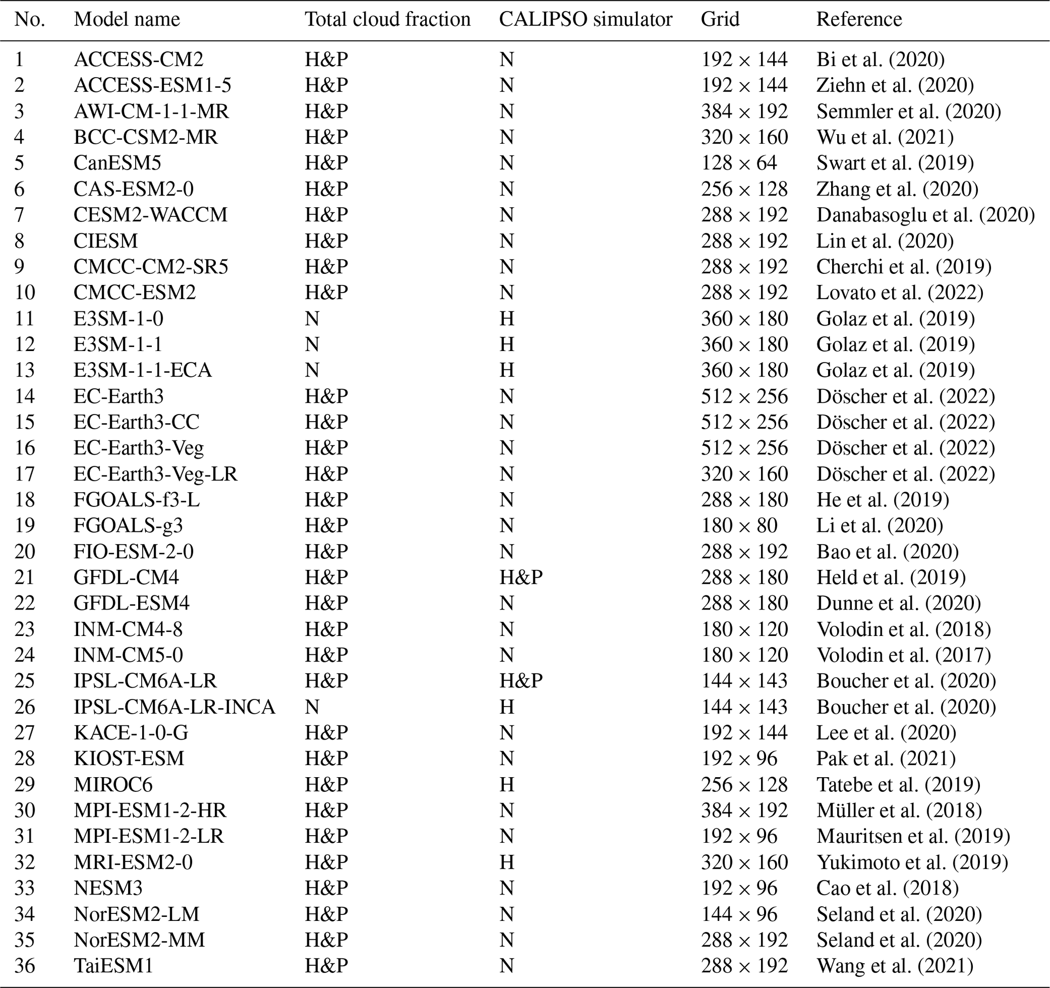
In order to examine the cloud cover trend in both historical and future periods, the cloud fraction data from 36 CMIP6 models are used in this work (Eyring et al., 2016). Considering the time span of all the models, the analysis is performed using the historical experiment driven by all forcings for the period from 1850 to 2014 and two future scenarios, the ssp245 (i.e., Shared Socio-Economic Pathway 2 and 2100 climate forcing level of 4.5 W m−2) and ssp585 (i.e., Shared Socio-Economic Pathway 5 and 2100 climate forcing level of 8.5 W m−2) experiments, for the period from 2015 to 2100 (O'Neill et al., 2016). ssp245 assumes a central pathway with continued historical tendencies, while ssp585 envisions optimistic but fossil-fueled development trends. Different future emission scenarios may provide further insights into the impacts of global climate change on cloud cover. Direct comparisons between the total cloud cover in models and satellite observations may be hampered by uncertainties due to the differences in cloud cover definitions and determination algorithms (Engström et al., 2015). Therefore, this investigation mainly employs the total and layered cloud fraction produced by the CALIPSO simulator, and the direct cloud cover simulations are used to verify the representativeness of the limited CALISPO simulator results. Three layered clouds are categorized according to the pressure thresholds of 440 and 680 hPa, i.e., high clouds (<440 hPa), middle clouds (680–440 hPa) and low clouds (>680 hPa). Note that clouds that straddle two (three) pressure layers are counted as two (three) cloud layers at the same time. Table 1 provides a list of CMIP6 models used in this study.
Table 1List of CMIP6 models used in this study. The data include monthly total cloud fraction (32 models) and monthly total, high-, middle- and low-cloud fraction produced by the CALIPSO simulator (eight models). All the model outputs during the historical period (1850–2014) and projected period (2015–2100) are used, excluding two CALIPSO simulator models that only contain the historical period. The labels H&P, H and N in the table indicate the data include both the historical and the projected periods, historical period only, and no data, respectively. Two types of scenarios (ssp245 and ssp585) are used in the projected period. All of the simulations have the variant label r1i1p1f1.
2.3 CVS classification and irradiance flux
CVS can be fairly complex with numerous conceivable configurations; therefore reducing its complexity into a handful of manageable classes requires simplification. In accordance with Oreopoulos et al. (2017), the two atmospheric boundaries of the ISCCP cloud categories, as specified in Sect. 2.1.2, are adopted as the basis for the three standard layers of CVS classifications in each CCCM cloud group profile. Since the CCCM product also gives the cloud base location, vertically separated cloud layers can be identified. When multiple overlapping clouds coexist inside the same standard layer or they contiguously span two or three standard layers, we treat them as one single-layer cloud. Under the above presumptions, 12 combinations illustrated in Fig. 1 are conceivable, including six single-layer clouds: isolated high clouds with base pressures <440 hPa (H), middle clouds with cloud base pressures <680 hPa and top pressures >440 hPa (M), and low clouds with top pressures >680 hPa (L), as well as contiguous clouds of H and M (H×M); M and L (M×L); and H, M and L (H×M×L) and six multi-layer clouds: non-contiguous clouds of H and M (HM); H and L (HL); M and L (ML); H, M and L (HML); H and M×L (HM×L); and H×M and L (H×ML). After classification, the cloud fraction of a certain CVS in each CCCM group profile can be derived.
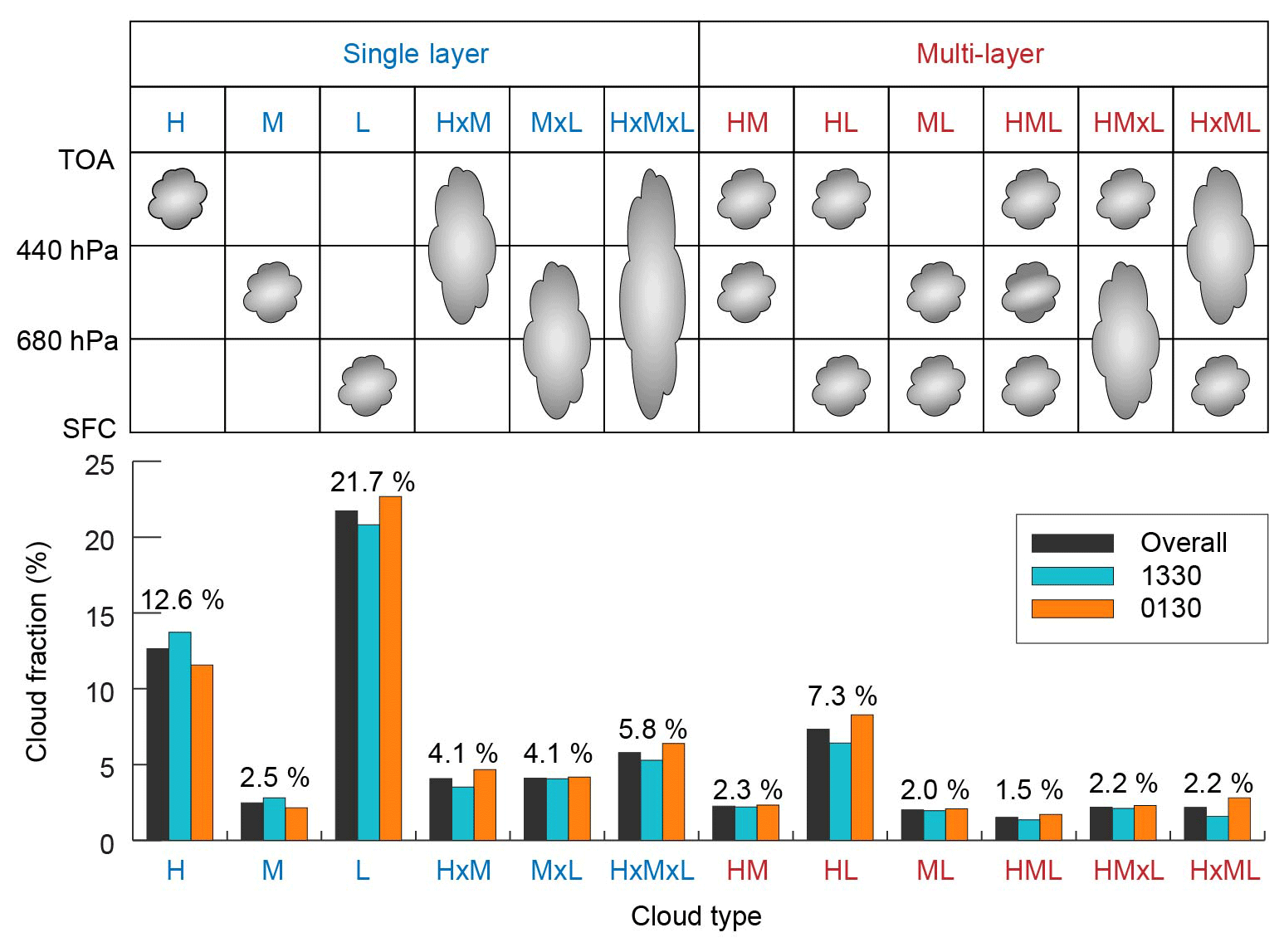
Figure 1Illustrative schematic of the 12 CVS categories defined in this study. Isobaric surfaces at 680 and 440 hPa are the two pressure boundaries for separating the cloud layers. The 4-year global area-weighted average cloud fraction of each CVS during the daytime (13:30 LST), nighttime (01:30 LST) and daytime + nighttime (overall) from 2007 to 2010 is presented. The values marked on the histogram indicate the overall time area-weighted average cloud fraction.
The radiative impacts of the total clouds and different CVS categories are investigated using the CCCM dataset. Since the satellites of the A-Train constellation used to generate the CCCM product are polar orbiting with fixed crossing times of approximately 01:30 and 13:30 local solar time (LST), the instantaneous solar irradiance is initially adjusted with the daily average solar insolation, , as applied by Haynes et al. (2013). The CRE at the TOA or surface is then calculated by
where F is the irradiance at the TOA or surface; the subscript x is either shortwave (SW) or longwave (LW); and the cloudy and clear indices denote cloudy-sky and clear-sky conditions, respectively. The superscripts ↓ and ↑ indicate downward and upward fluxes, respectively. The sum of SW and LW CRE gives the net CRE. The difference between the CRE at the TOA and the surface is the CRE within the atmosphere.
The vertical irradiance profile provided by the CCCM product is used to obtain the heating rate (HR) profile, and the HR at a certain layer is computed by
where T is the layer temperature, t is time, F is the irradiance, p is the pressure, cp=1004 is the specific heat capacity of air at constant pressure, and g=9.81 m s−1 is the gravitational constant. The subscripts upper and lower denote, respectively, the upper and lower boundary of a layer, and x is either SW or LW. The unit of HR is converted to K d−1.
After calculating the HR, the cloud heating rate (CHR), which denotes the HR between cloudy-sky and clear-sky conditions, is represented by
where the subscript x is either SW or LW, and the superscripts cloudy and clear denote cloudy-sky and clear-sky conditions, respectively. The sum of SW and LW CHR indicates the net CHR.
Note that when we examine the CRE and CHR for a specific CVS class, the cloud group containing only one CVS class with a cloud fraction of 100 % is considered. In terms of the spatial distributions, the cloud fraction and CRE calculated in a CERES footprint are further monthly averaged to a grid of .
3.1 CCCM observations of CVS
Before delving into the CCCM product, we first assess its cloud fraction in comparison to the data from the Level-2B GEOPROF-LIDAR. Although Ham et al. (2017) have conducted a 4-month thorough comparison between these two products, the findings are only applicable to the previous version of the CCCM data (RelB1). Overall, the 4-year assessments in Fig. S1 in the Supplement indicate that the CCCM and GEOPROF-LIDAR products capture quite comparable features, and the temporal correlations are extremely strong for both total and different types of cloud cover. However, biases between these two products cannot be ignored, notably for the middle cloud, which has a global average cloud fraction bias of 5.74 %. These biases are mainly induced by differences in cloud mask algorithms between the CCCM and GEOPROF-LIDAR discussed in Sect. 2.1.2, despite their employing of the same satellite products (Ham et al., 2017).
The spatial distributions of the 12 CVS categories are shown in Fig. 2. Although there exist slight differences in daytime and nighttime cloud fractions of the 12 CVSs, the magnitudes are consistent (Fig. 1); thus we merely show the average values here. The statistical results demonstrate that single-layer clouds of L, H and, to lesser extent, H×M×L, as well as the multi-layer cloud of HL, occur frequently, whereas the other eight CVSs all have relatively lower cloud fractions, with area-weighted averages of less than 5 %. Basically, H distributes with latitudes, with its high values in the Tropics across the west-central Pacific Ocean warm pool, Indonesia, western Africa and central South America. The Tibetan Plateau, which is dominated by high topography, is another region with a high H fraction. In contrast, L is distributed throughout the low-value zones of H and shows a clear land–ocean difference with very low values over land, except for some regions in the Northern Hemisphere mid-to-high latitudes. The L class has very high values over oceans globally, except where the H class is prevalent. The distributions of HL and H×M×L generally follow a similar pattern as H, apart from the low values over the Tibetan Plateau due to the absence of low-level clouds. For the eight infrequent CVSs (average cloud fraction <5 %), their spatial patterns resemble the feature of H×M×L, excluding the high values of H×M over the Tibetan Plateau and Antarctica caused by high terrain. In conclusion, the spatial patterns of these 12 CVSs reveal consistent distributions with well-known cloud top height/pressure characteristics (Marchand et al., 2010; King et al., 2013) and, for the single-layer clouds, documented cloud regimes from approaches (Tselioudis et al., 2013, 2021; Unglaub et al., 2020). However, the quantitative cloud fractions of the various CVS types provided here have not previously been achievable with passive satellite sensors.
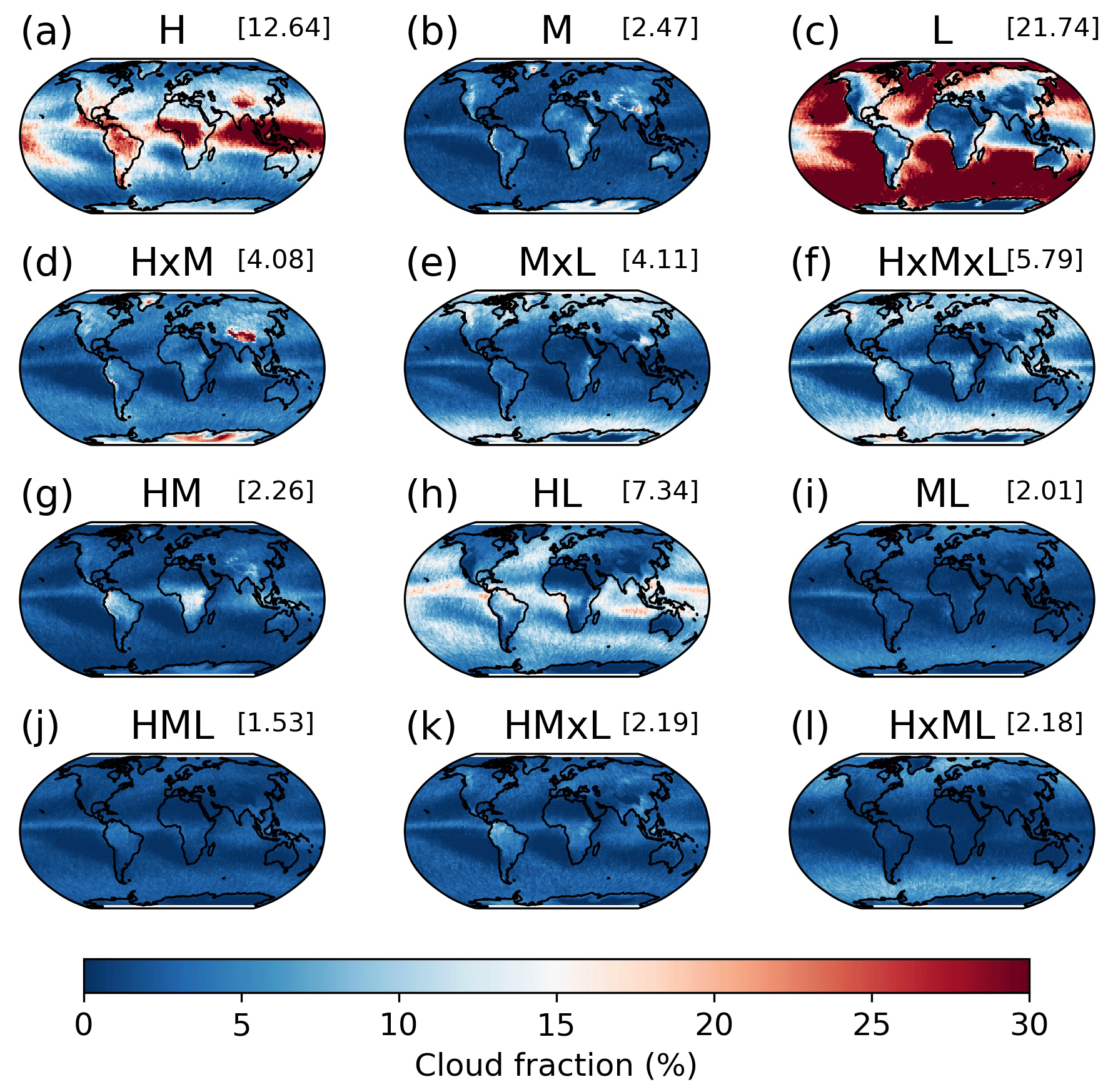
Figure 2Spatial distributions of the 4-year (2007–2010) average cloud fraction of (a) H, (b) M, (c) L, (d) H×M, (e) M×L, (f) H×M×L, (g) HM, (h) HL, (i) ML, (j) HML, (k) HM×L and (l) H×ML. The value above each subfigure denotes the area-weighted average.
For the six overlapping cloud types, it is more challenging to derive the cloud radiative effect. However, their fractions are much lower than the ones of the single-layer clouds. Figure 3 shows the spatial distributions of the single-layer and multi-layer clouds, as well as their ratio. In the global average, single-layer clouds are 3.74 times more frequent than multi-layer clouds. This ratio exhibits considerable regional variations that are associated with clearly distinguishable regimes. In the time average, nowhere are multi-layer clouds more frequent than single-layer clouds. Over tropical convective zones, multi-layer clouds are almost as frequent as single-layer clouds. A reason for this is that cirrus clouds from either large-scale ascents or dissipating deep convections are ubiquitous in these regions, both in the absence (Fig. 2a) and in the presence (Fig. 3c) of low-level clouds below the cirrus. In contrast, near the descending branch of the Hadley cell in both hemispheres, single-layer clouds are often an order of magnitude more frequent than multi-layer clouds. There, the prevalent subsidence is unfavorable for the formation of mid- or upper-level clouds (Yuan and Oreopoulos, 2013). The large ratio values over Antarctica and Greenland are influenced by the descending branch of the polar circulation. In brief, the single-layer clouds prefer regions with a stable troposphere, while the multi-layer clouds favor the regions with strong ascents.
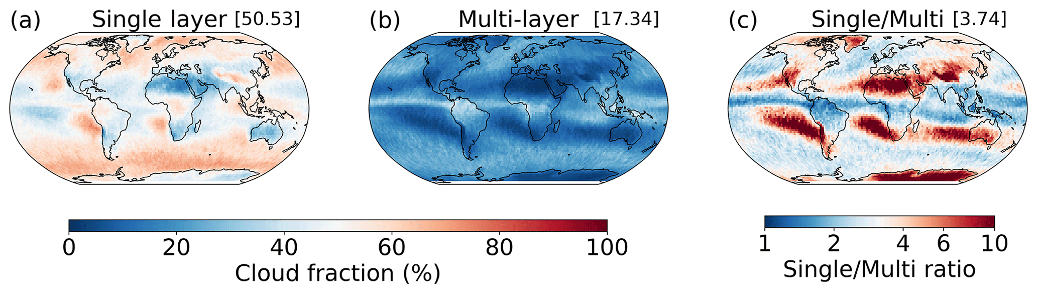
Figure 3Spatial distributions of the 4-year (2007–2010) average (a) single-layer cloud fraction, (b) multi-layer cloud fraction, and (c) the ratio of time-averaged single-layer cloud fraction to the multi-layer cloud fraction. The value above each subfigure denotes the area-weighted global 4-year average.
In addition to the global horizontal distributions, another concern is the vertical extent of each type of CVS. These, provided by the top and base heights, are shown as global averages in Fig. 4. In the presence of high-level clouds, different CVSs present distinctive top heights. When the high-level clouds occur alone or overlap thinner low-level clouds (average geometric thickness ≤1 km), the cloud tops exceed 12 km (H, HM and HL), primarily in the Tropics throughout the west-central Pacific Ocean warm pool, Indonesia, western Africa and central South America. However, the cloud tops drop to approximately 10–11 km when thicker low-level clouds (average geometric thickness ≥2 km) are overlapped by high clouds (e.g., HML and HM×L), mainly across equatorial and mid–high latitudes. The average cloud top of deep convective clouds (H×M×L) distributed mostly over equatorial and mid–high latitudes is >11 km but lower than the isolated H. The cloud tops are much lower (<10 km) when the high-level clouds and mid-level clouds are contiguous (e.g., H×M and H×ML), and they are generally spread over high altitudes and mid–high latitudes.
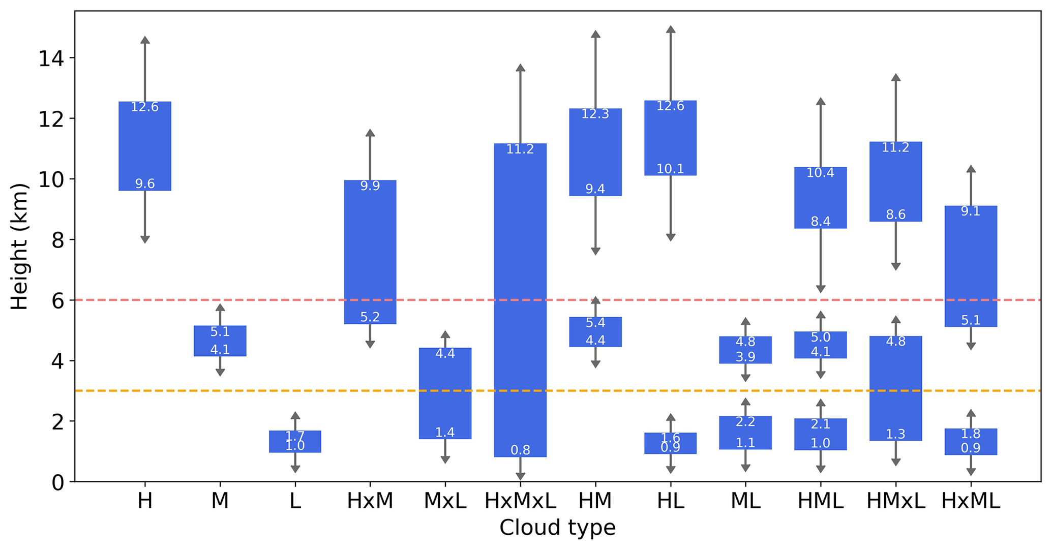
Figure 4The 4-year (2007–2010) global average cloud vertical locations (cloud top and base heights) of the 12 CVSs. The upper (lower) values within the boxes indicate the cloud top (base) heights. Standard deviations are depicted by the arrows. The height here refers to the altitude above sea level. The horizontal yellow and red lines represent heights at 3 and 6 km, respectively, equivalent to the global average height of the isobaric surface of about 680 and 440 hPa.
Morphological differences in low-level clouds among the CVSs are also observed. The cloud base heights are higher (>1 km) when the low-level clouds connect with the mid-level clouds (e.g., M×L and HM×L), mostly occurring across equatorial and mid–high latitudes. Contrarily, deep convective clouds (H×M×L), which prevail over the same regions as M×L and HM×L, have the lowest base height.
3.2 CCCM observations of CRE
The CCCM product makes use of the combination of cloud profiles from active satellites, cloud optical properties from MODIS and broadband radiation fluxes from CERES to compute radiative flux profiles using radiative transfer modeling. Figure 5 shows the total SW, LW and net CREs at the TOA and surface as well as within the atmosphere as provided by 4 years of CCCM data from 2007 to 2010. Overall, this matches the global patterns of CREs examined in previous studies using other datasets (Allan, 2011; Dolinar et al., 2019), although values deviate somewhat. In total, clouds act to cool the Earth atmosphere system with a global average net TOA CRE of −18.7 W m−2, which is due to the cloud albedo effect. Over northern Africa and other bright surfaces (e.g., Greenland, the Arctic, Antarctica), there is a slight warming at the TOA, and the cloud greenhouse effect dominates. The SW CRE manifests primarily as surface cooling, with an average residual heating of 4.69 W m−2 within the atmosphere. This heating effect is partly related to an enhanced SW absorption by water vapor in the atmosphere in cloudy compared to clear skies (Sohn et al., 2006; Allan, 2011) and partly to SW absorption by the clouds themselves (Slingo and Schrecker, 1982). The SW CRE within the atmosphere is homogenous globally, so the spatial pattern of net CRE within the atmosphere is driven by LW. At the surface, net CRE is dominated by SW cooling, except over the poles, which are warmed by LW heating.
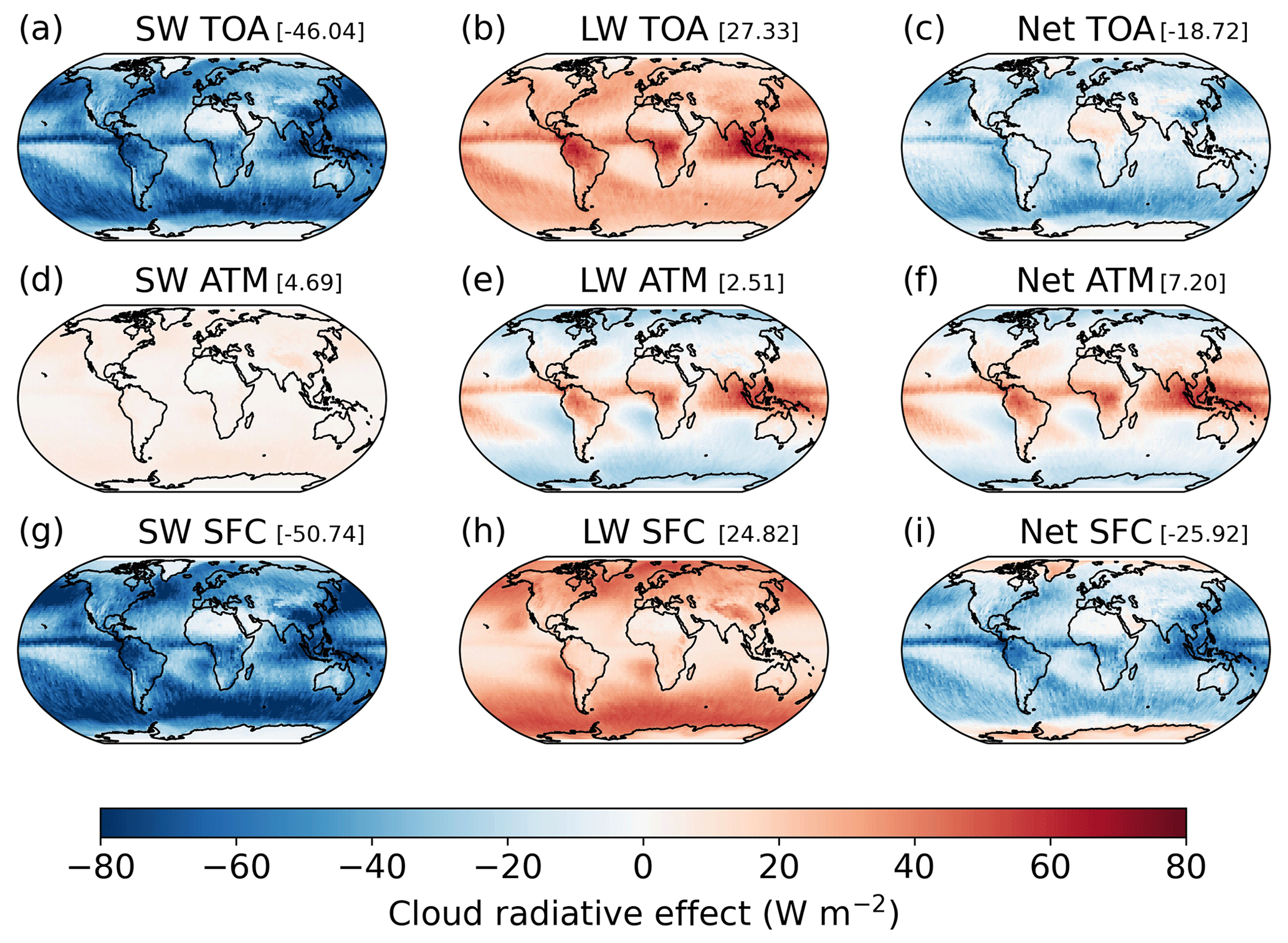
Figure 5Spatial distributions of the 4-year (2007–2010) average SW, LW and net CREs (a–c) at TOA, (d–f) within the atmosphere and (g–i) at the surface. The value above each subfigure denotes the area-weighted average.
Given the systematic differences in the total opacities and thermal emissions caused by vertical extent and temperature-dependent cloud phase, it is evident that different CVSs influence the radiative flux for both SW and LW within the atmosphere in distinct ways. The geographic variations in prevalent CVSs over different regions cause the spatial pattern of CRE in Fig. 5. Therefore, quantifying the global average CREs induced by various types of CVSs is valuable. Figure 6 shows the global average SW, LW and net CREs at the TOA, within the atmosphere and at the surface for the 12 classified CVSs.
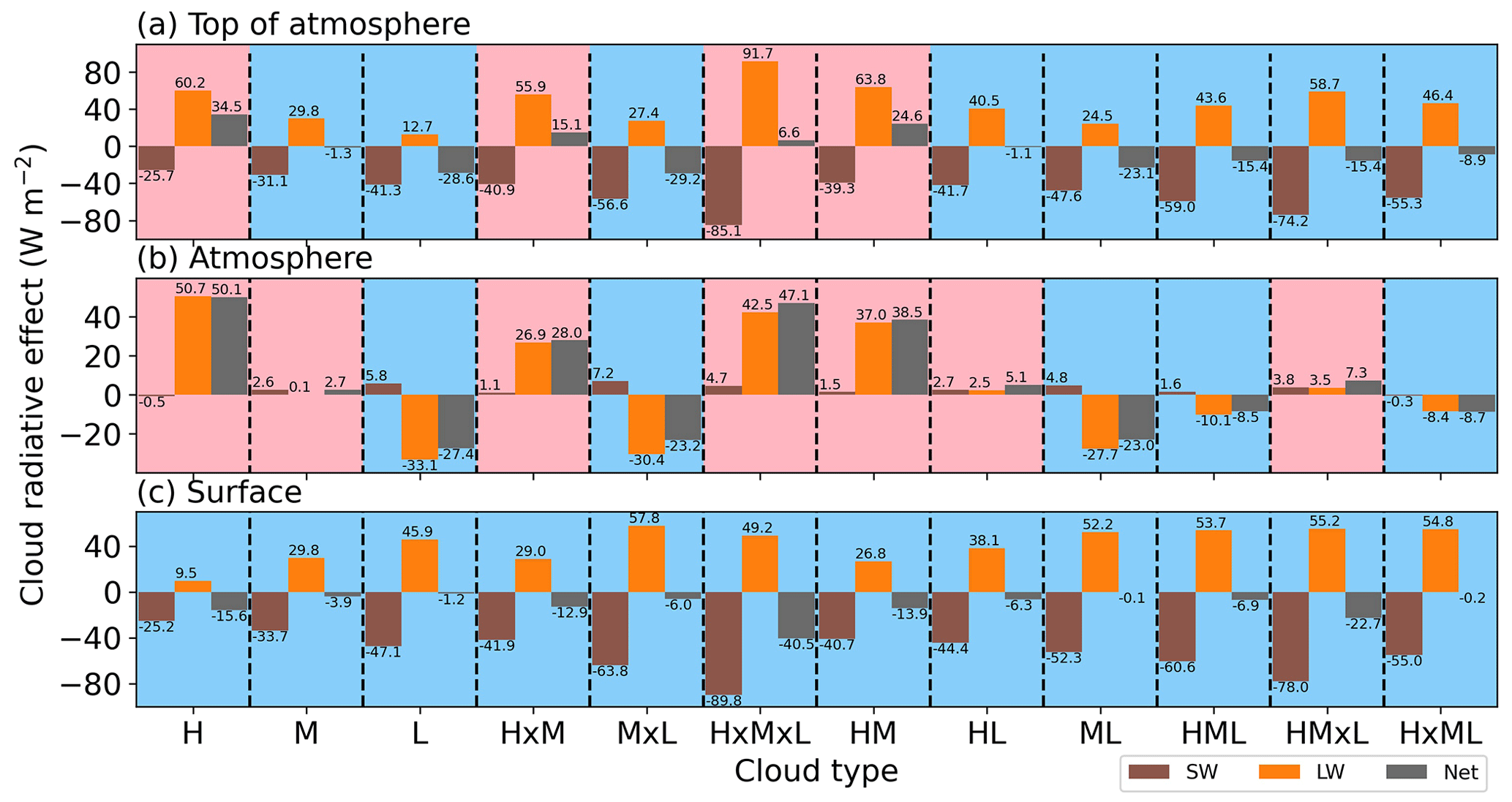
Figure 6The 4-year (2007–2010) global average SW, LW and net CREs of the 12 CVSs (a) at TOA, (b) within the atmosphere and (c) at the surface. The blue and red backgrounds in each sub-box indicate cooling and warming effects, respectively.
In terms of SW CRE, the magnitude of each CVS is similar at the surface and TOA, with a relatively small value within the atmosphere. The minor positive values of SW CRE within the atmosphere are due to the increased atmospheric path length for radiation reflected by clouds that caused an enhanced absorption by water vapor, but for some high-level clouds (e.g., H and H×ML), the reflection at high altitudes instead decreases the SW absorption by the atmosphere that induces tiny negative values. At the TOA and surface, all types of CVSs exert cooling effects in the SW. In general, low-level clouds have stronger SW CREs than high-level clouds due to the generally vertically decreasing profile in cloud water content and due to cloud-phase differences. When they are overlapped or connected with upper-level clouds, the SW CREs further increase as the vertically integrated water content and thus optical thickness increases. The deep convective clouds of H×M×L with an average geometric thickness >10 km have, as expected, the strongest albedo effect ( W m−2).
Compared to SW, LW CRE exhibits more complex features. At the TOA and surface, all types of CVSs act as warming effects in LW, but the magnitude differs a lot. At the TOA, since the LW CRE highly depends on the temperature difference between the surface and cloud top, CVSs containing high-level clouds all have a strong LW CRE (>40 W m−2), notably for the H×M×L with its value >90 W m−2. On the contrary, LW CRE at the surface greatly depends on the cloud base thermal emission. Therefore, the CVSs containing low-level clouds all have a strong LW CRE at the surface (>38 W m−2), whereas the H with the highest cloud base presents the weakest surface LW CRE (<10 W m−2). As the LW CREs at the TOA and surface are quite dissimilar, the LW CREs within the atmosphere display a wide range among all the CVSs. The clear distinction is that the H causes LW radiative warming within the atmosphere, while the L causes LW radiative cooling. The LW CREs generated by the clouds between the locations of L and H or the combination of the two can be offset to some extent.
The net CRE, which combines both SW and LW, indicates whether a specific type of CVS has an overall warming or cooling effect. At the TOA, four CVSs have warming effects, all of which include high-level clouds, while eight CVSs have cooling effects, and most of them contain low-level clouds. For M or HL, SW and LW cancel out almost entirely. Within the atmosphere, there are seven CVSs that in the net warm the atmosphere, while five CVSs cool it. At the surface, all types of CVSs have net cooling effects, as the reduction in SW reaching the surface is larger than the increase in downwelling LW. However, in terms of spatial distribution, there are positive values of net CRE observed at the surface over bright areas (e.g., Greenland, the Arctic, Antarctica) (Fig. 5i), where the cloud greenhouse effect prevails. Nevertheless, when examining the global average, the net positive CREs of cloud types that dominate over these bright regions are rather small in magnitude compared to the average albedo effects of the same cloud types over most other regions, ultimately resulting in net cooling at the surface. We conclude that these intriguing discrepancies in the CREs of all kinds of CVSs contribute to large uncertainties in estimating changes in the radiative budget when the spatial patterns of CVS change.
Apart from the integral CREs within the atmosphere, the CHR profiles of 12 CVS types are further illustrated in Fig. 7, which can provide detailed profiles of how clouds vertically affect radiative heating as provided by the CCCM dataset. Overall, the net CHR profiles are driven by the LW component, and the CHR profiles of multi-layer clouds are more curved and complex than those of single-layer clouds. Regarding SW, all the CVSs exert similar characteristics, which are shown as heating near the cloud layers and cooling beneath the clouds. Due to the SW absorption within the upper parts of some optically thick clouds (e.g., M×L and H×M×L), the SW cooling starts to appear in the middle and lower portions of the clouds. Concerning LW, the heating below the cloud layers is due to the absorption of LW radiation emitted from the surface or the lower clouds below, while the LW cooling near and above the cloud layers is the result of radiative emissions by the clouds. Strong greenhouse effects are produced by ample ice particles inside the H, exhibiting inconsistent characteristics distinguished from the other CVSs and even heating all levels below the cloud top. In conclusion, the SW albedo effects, LW greenhouse effects and the interactions between cloud layers result in rather complex radiative profiles, contributing to manifold atmospheric thermal stratifications. The precise assessment of these stratifications is inextricably linked to the accurate observation of cloud properties, especially the detection of vertically overlapping clouds.
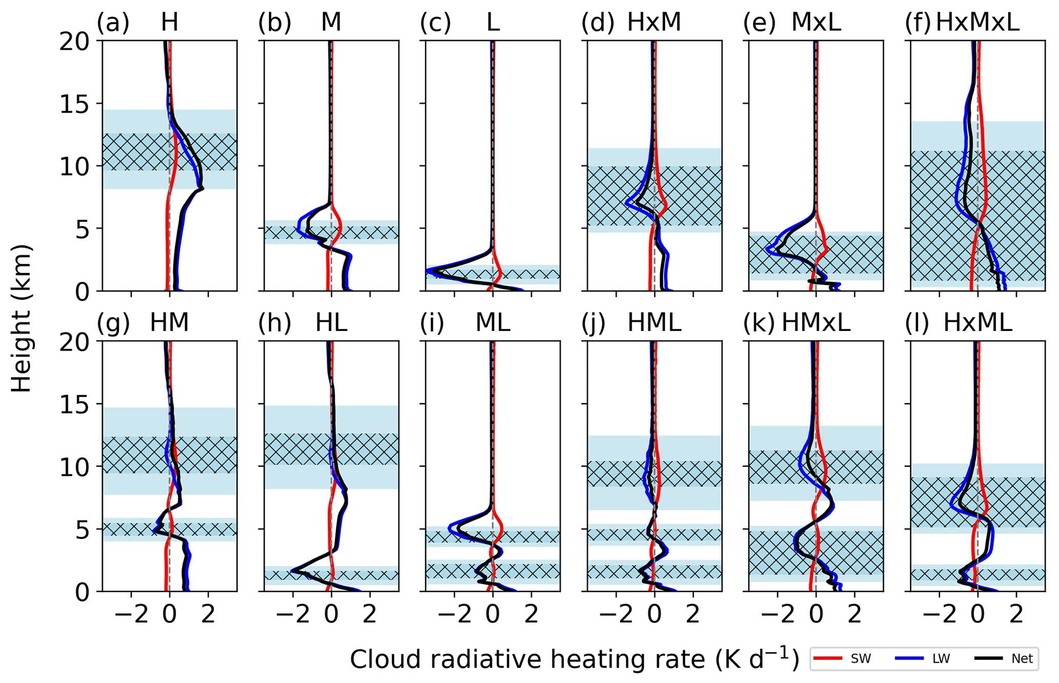
Figure 7The 4-year (2007–2010) global average profiles of SW, LW and net CHRs for (a) H, (b) M, (c) L, (d) H×M, (e) M×L, (f) H×M×L, (g) HM, (h) HL, (i) ML, (j) HML, (k) HM×L and (l) H×ML. The red, blue and black lines denote SW, LW and net CHRs, respectively. The darker blue mesh rectangles represent the average cloud locations, while the lighter blue rectangles above (below) the average cloud locations represent the standard deviations of the cloud top (base) heights. The height here refers to the altitude above sea level.
3.3 Trends and projections of CVS from CMIP6
In light of the widely disparate radiative effects of different kinds of CVSs, the response of CVS to a warming climate appears to be particularly important. However, how the CVS changes during the historical period and future projections remains poorly constrained. Some aspects have been documented in Norris et al. (2016) from passive satellite sensors. In this section, the trends in total, high-, middle- and low-level cloud fractions from 1850 to the end of this century are analyzed based on CMIP6 models. The historical experiment driven by all sorts of forcing for the period from 1850 to 2014 and two future scenarios (the ssp245 and ssp585 experiments) for the period from 2015 to 2100 are used. Furthermore, we investigate whether the global spatial distribution of the dominating cloud type will change as a result of climate warming.
Because GCMs only parameterize cloud fraction, the performance of the CMIP6 models is initially assessed with CCCM observations. Figure 8 presents scatterplots of the monthly average cloud fraction between the MME using the CALIPSO simulator diagnostics available from eight CMIP6 models and the CCCM datasets, including total, high, middle and low clouds between 2007 and 2010. Land and ocean regions are separated. The results indicate that CMIP6 models in general capture the monthly mean cloud fraction for both total and layered clouds rather well, especially over the ocean with correlation coefficients ≥0.9. Cloud fraction in CMIP6 is systematically underestimated due to the ability of two active satellites (CALIPSO and CloudSat) in CCCM to retrieve more clouds than CALIPSO alone. Although this underestimation mainly occurs over the tropical regions, the correlations against CCCM are even stronger than in high latitudes (Fig. S2). It is concluded that the CMIP6 models perform well in simulating the cloud fraction for both the total and the layered clouds, implying that estimating the historical and projected cloud fraction using CMIP6 is reliable. Additionally, since there are only two models (GFDL-CM4 and IPSL-CM6A-LR) available for the future period, it is crucial to assess whether these two models have representation comparably good to the MME mean. Figure S3 compares the total, high-, middle- and low-cloud fractions of the two CMIP6 CALIPSO simulator MMEs with the total eight CALIPSO simulator MMEs for the historical period from 1850 to 2014. Figure S4 further analyzes the total cloud fraction correlations between the two CALIPSO simulator MMEs and 32 model MMEs for four different periods from the past to the future. The results demonstrate that for both historical and future periods, the two models, for which CALIPSO simulator output is also available for future scenarios, have a fair representation of the simulated cloud fractions over both land and ocean regions. Although the cloud fraction from the direct simulation of the 32 GCMs is defined differently from that in CALIPSO simulators, they are still highly correlated. Besides the intercomparison between the models, a similar assessment result as in Fig. 8, but the relationship between the average of two models (GFDL-CM4 and IPSL-CM6A-LR) and CCCM during 2007–2100, is depicted in Fig. S5.
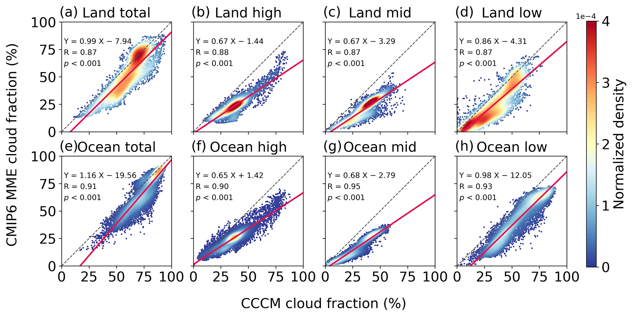
Figure 8Normalized density plots of the 4-year (2007–2010) monthly average (a, e) total, (b, f) high-, (c, g) middle- and (d, h) low-cloud fractions estimated from the eight CMIP6 CALIPSO simulator MMEs versus the CCCM measurements over land and the ocean, respectively. The regressions are represented by the red lines. The regression function, correlation coefficient (R) and p value are given in each subplot.
Time series of annual average cloud fraction based on the two CMIP6 models from 1850 to 2100 are presented in Fig. 9, including two scenarios of ssp245 and ssp585 for the future. Here, four time periods are specifically focused on to understand the temporal variations, which include the baseline (1994–2014), near term (2021–2040), midterm (2051–2070) and long term (2081–2100). The spatial differences between the future periods under ssp585 (ssp245) and the historical baseline are illustrated in Fig. 10 (Fig. S6). The results show that the projected total cloud fraction decreases faster over land than over the ocean. High clouds over oceans increase dramatically, while other types of clouds over land and the ocean all continue to decrease, which helps to almost offset the reduction in the oceanic total cloud fraction. Though the global average middle- and low-cloud fractions both decrease over land and the ocean in the future, the low-cloud fractions over the tropical ocean and the Arctic show a significant increase. The increase in oceanic high clouds is spatially concentrated across the tropical Pacific Ocean and the high latitudes, emphasizing the ensuing positive cloud feedback generated by the increased ice clouds. The decreasing trend difference between continental and oceanic total cloud cover is also influenced by spatial patterns; cloud fraction over land (except the polar regions) consistently decreases, whereas the opposing tendency between high and low latitudes over the ocean offsets the global average.
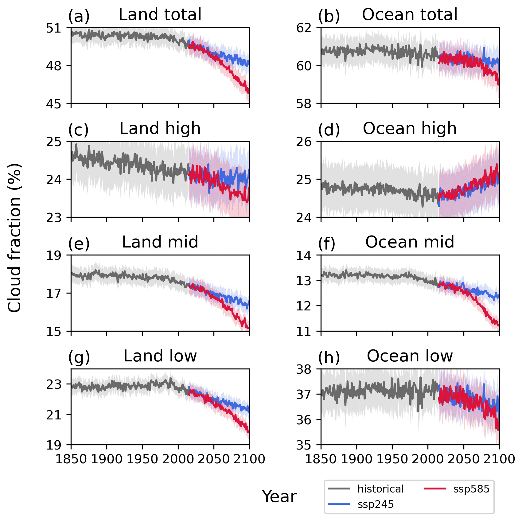
Figure 9Time series of annual area-weighted average (a, b) total, (c, d) high-, (e, f) middle- and (g, h) low-cloud fractions from two CMIP6 CALIPSO simulator MMEs during 1850–2100 over land and the ocean, respectively. The future projections from 2015 to 2100 are based on two scenarios of ssp245 and ssp585. The shadows indicate the standard deviations.
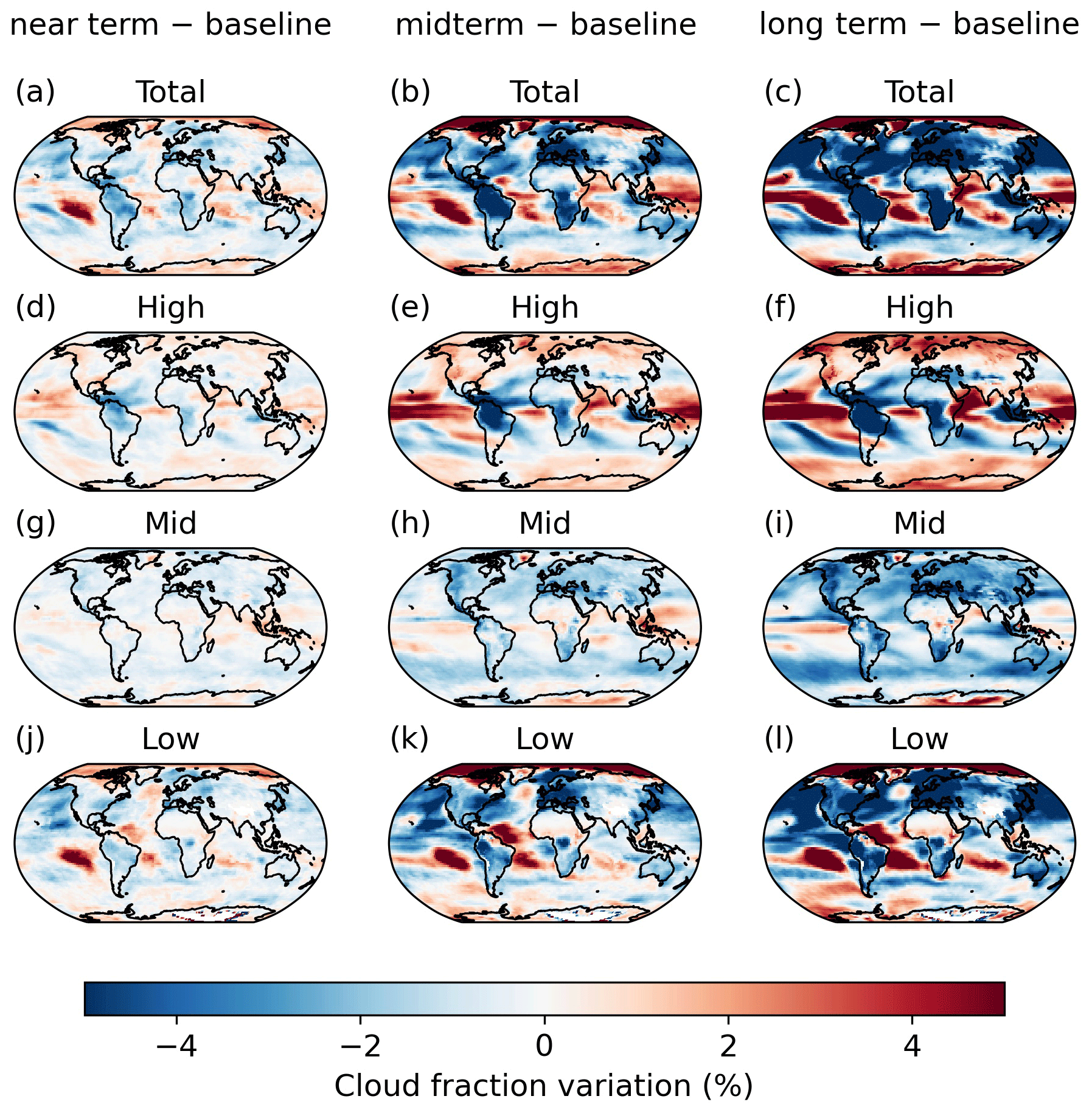
Figure 10Spatial variations in annual average (a–c) total, (d–f) high-, (g–i) middle- and (j–l) low-cloud fractions in the near term (2021–2040), midterm (2051–2070) and long term (2081–2100) periods compared to the baseline (1994–2014) period under ssp585.
For the near term, there are only slight differences in the total cloud fraction over land between ssp245 and ssp585, but for the middle and long term, the cloud response becomes more sensitive to different anthropogenic forcing. The total cloud fraction over the ocean, however, only shows a discernible difference between the two scenarios in the long term. The different layered cloud fractions exhibit the same time series feature as the total cloud fraction over land. Over the oceans, the high cloud shows small differences between the two scenarios over all the projected periods, while the low cloud only shows a discernible difference in the long term. Although the oceanic middle-cloud fraction changes significantly over the middle and long terms, its small value means that it contributes little to the total cloud cover. The combined changes in the high and low clouds over the ocean mainly result in the time series features of the total cloud fraction.
As the above analysis demonstrates, the changes in total cloud cover and distinct types of cloud cover are noticeable in the context of climate change. The interesting question that follows is could climate warming and anthropogenic forcing change the driving cloud type in a certain area? Here, we analyze the correlations between the cloud types and the total cloud cover using historical forcing and future scenarios. Two correlation coefficient thresholds of 0.66 and 0.9 with p value <0.05 are employed, which means likely positive correlation and very likely positive correlation, respectively (Chen et al., 2021). When only one cloud type is correlated with the total cloud fraction, we presume that only this cloud drives the total cloud cover. When two or three cloud types are simultaneously correlated with the total cloud fraction, we assume that the total cloud cover is driven by these several cloud types together.
Figure 11 depicts the results with a correlation coefficient >0.66, and the results with a correlation coefficient >0.9 are displayed in Fig. S7. Over the ocean, the changes in total cloud fraction are mainly governed by low cloud cover, with the exception of the tropical Pacific Midwest and the Indian Ocean, where high clouds or a combination of high and middle clouds dominate the total cloud cover change. Over land, the regional differences are more pronounced. At high northern latitudes, middle and low clouds together drive the total cloud cover. In low-latitude regions, high clouds have a greater influence on the total cloud cover, and some regions, such as South America, South and Central Africa, and Indonesia, are synchronously affected by middle and low clouds. In the Antarctic region, the total cloud fraction is primarily affected by the middle cloud, which has a clearer signal when the correlation coefficient threshold is increased to 0.9, as seen in Fig. S7. Moreover, by comparing the results of different periods and scenarios, we can conclude that climate change and human activities have little impact on this spatial pattern.
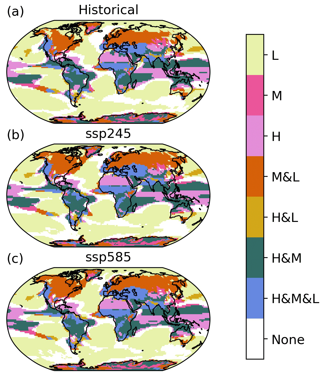
Figure 11Spatial distributions of the clouds with a positive correlation coefficient >0.66 (p value<0.05) with the total cloud fraction during (a) the historical period (1850–2014) as well as the projected period (2015–2100) under (b) ssp245 and (c) ssp585. The labels L, M and H indicate that only one certain cloud type is correlated with the total cloud fraction, while the labels connected by & imply that two or three cloud types are simultaneously correlated with the total cloud fraction, and the label None means no cloud is correlated with the total cloud fraction.
In the present study, we conduct a comprehensive analysis of CVS at a global scale using the CCCM product from 2007 to 2010 that combines satellite observations from CERES, CALIPSO, CloudSat and MODIS. To capture the richness of CVS with minimal sacrifice and simplify the complex configurations, cloud layers in a particular vertical profile that occupy one, two or three standard vertical layers are considered, and overall, a total of 12 distinct CVS types are categorized. The detailed statistical morphology and spatial distribution of each CVS are investigated. To better understand cloud radiative forcing, the global average CRE and CHR profile of each CVS type are quantified. In addition, this work uses CMIP6 outputs to assess the long-term changes in cloud cover and to explore variations in low-, middle-, and high-level cloud fractions during the historical and projected periods in the context of climate change.
To date, because the CCCM RelD1 is a new product providing the vertical profile of the clouds, a concise comparison with the 2B-GEOPROF-LIDAR is performed first to ensure the reliability of the dataset. In general, the spatial characteristics captured by the CCCM and 2B-GEOPROF-LIDAR products are quite similar. The global average total cloud fraction bias between these two products is −1.15 %, with the middle clouds showing a notable bias of 5.74 % compared to other layers. These discrepancies exist mostly owing to the differences between the algorithms of the two products. By and large, CCCM is a viable option in exploring CVS due to its high vertical resolution and reasonable accuracy.
The 4-year quantitative analysis of cloud fraction indicates that single-layer clouds such as L, H and H×M×L, as well as the multi-layer cloud of HL, occur more frequently than the other types of CVSs. Generally, H is distributed according to latitude, with high values seen in the Tropics around Indonesia, the western and central Pacific Ocean warm pool, western Africa, and central South America. Another region characterized by a high fraction of H is the Tibetan Plateau, where high topography dominates. In turn, L has a distinct land–ocean contrast and is mainly located throughout the low-value zones of H. The distributions of HL and H×M×L exhibit a similar pattern as H, except for their low values over the Tibetan Plateau resulting from the lack of low-level clouds. On average, single-layer clouds are 3.74 times more frequent than multi-layer clouds. This ratio demonstrates significant geographic variations associated with clearly identifiable regimes, implying that overlapping clouds are regionally different. As the most prevalent multi-layer cloud, HL is distinguished by its complicated vertical structure and significant spatial pattern. Aside from the global distributions, the morphology of each CVS, including the cloud top and base locations, is concluded, which has received scant attention in prior studies, especially for the overlapping clouds.
Moreover, the CCCM product also provides estimates of the radiative budget from the perspective of CVS. Distinct influences of various CVSs on radiative flux for both SW and LW are evident due to the systematic opacity and thermal emission differences caused by vertical extension and temperature-dependent cloud phase. In terms of SW, all types of CVSs act as cooling effects at the TOA and surface, with a relatively small absorption within the atmosphere. Low-level clouds have stronger SW CREs than high-level clouds due to the liquid–ice-phase differences, and when they are overlapped or connected with upper-level clouds, the SW CREs further increase. LW CRE displays more intricate details when compared to SW. LW CRE highly depends on the temperature difference between the surface and cloud top at the TOA and greatly depends on the cloud base thermal emission at the surface. Therefore, CVSs containing high-level (low-level) clouds have a strong LW CRE at the TOA (surface). The LW CREs within the atmosphere imply a wide range across all CVSs owing to the large differences between the TOA and surface. As a result, the net CRE, which is the synthetical performance of SW and LW, exhibits varying warming or cooling effects depending on the CVS. From the perspective of the vertical profile, the LW component drives the net CHR, and the CHR profiles of multi-layer clouds are more curved and complex than those of single-layer clouds. The SW albedo effects and LW greenhouse effects, as well as the interactions across cloud layers, provide quite complex radiative profiles that contribute to a variety of atmospheric thermal stratifications.
The response of CVS to a warming climate appears to be especially crucial in regard to the widely diverse radiative effects of different types of CVSs. Therefore, the variations in total, high-, middle- and low-level cloud fractions from 1850 to 2100 are analyzed based on CMIP6 models, and the historical experiment during the past period and two scenarios (ssp245 and ssp585) during the future period are considered. Here, we find that the CMIP6 models can capture the features of different cloud types well when validated by the CCCM data. According to the findings, the projected total cloud fraction decreases faster over land than over the ocean. The high clouds over the ocean increase considerably, but other types of clouds over land and the ocean continue to decrease, helping to counteract the decrease in the total cloud fraction over the ocean. Overall, the changes in total cloud cover and distinct types of cloud cover are noticeable in the context of climate change and respond differently to anthropogenic forcing. Based on correlation analysis, it is believed that the spatial pattern of cloud types may not be significantly altered by climate change, and rather the cloud fractional coverage per type is affected.
This work provides a detailed survey of the global-scale distribution, morphology and CRE of 12 different CVSs using joint satellite observations, but the 4-year result is insufficient to accurately describe the climatological characteristics. Although the long-term variations in CVS are depicted by the CMIP6 models, it is still a challenge to understand the long-term trend of the intricate cloud structure using the relatively crude and simple classification in the models.
The CCCM RelD1 data were obtained from https://opendap.larc.nasa.gov/opendap/CERES/CCCM/Aqua-FM3-MODIS-CAL-CS_RelD1/contents.html (Kato et al., 2021). The 2B-GEOPROF-LIDAR data are available from https://www.cloudsat.cira.colostate.edu/data-products/2b-geoprof-lidar (Mace and Zhang, 2014). The CMIP6 data were taken from https://esgf-data.dkrz.de/search/cmip6-dkrz/ (Eyring et al., 2016).
The supplement related to this article is available online at: https://doi.org/10.5194/acp-23-8169-2023-supplement.
This study was conceived by HL and JQ with contributions from all authors. HL performed the research and prepared the manuscript, with comments from JQ and YH.
At least one of the (co-)authors is a member of the editorial board of Atmospheric Chemistry and Physics. The peer-review process was guided by an independent editor, and the authors also have no other competing interests to declare.
Publisher's note: Copernicus Publications remains neutral with regard to jurisdictional claims in published maps and institutional affiliations.
We thank the two anonymous reviewers for their constructive comments that have helped us to improve the paper.
This research has been supported by the National Natural Science Foundation of China (grant nos. 42027804, 41775026, 41075012 and 40805006) and the Innovation Group Project of the Southern Marine Science and Engineering Guangdong Laboratory (Zhuhai) (grant no. 311022006). Hao Luo has been supported by the China Scholarship Council.
This paper was edited by Martina Krämer and reviewed by two anonymous referees.
Allan, R. P.: Combining satellite data and models to estimate cloud radiative effect at the surface and in the atmosphere, Meteorol. Appl., 18, 324–333, https://doi.org/10.1002/met.285, 2011.
Bao, Y., Song, Z., and Qiao, F.: FIO-ESM Version 2.0: Model Description and Evaluation, J. Geophys. Res.-Oceans, 125, e2019JC016036, https://doi.org/10.1029/2019JC016036, 2020.
Betts, A. K. and Harshvardhan: Thermodynamic constraint on the cloud liquid water feedback in climate models, J. Geophys. Res.-Atmos., 92, 8483–8485, https://doi.org/10.1029/JD092iD07p08483, 1987.
Bi, D., Dix, M., Marsland, S., O'Farrell, S., Sullivan, A., Bodman, R., Law, R., Harman, I., Srbinovsky, J., Rashid, H. A., Dobrohotoff, P., Mackallah, C., Yan, H., Hirst, A., Savita, A., Dias, F. B., Woodhouse, M., Fiedler, R., and Heerdegen, A.: Configuration and spin-up of ACCESS-CM2, the new generation Australian Community Climate and Earth System Simulator Coupled Model, Journal of Southern Hemisphere Earth Systems Science, 70, 225–251, https://doi.org/10.1071/ES19040, 2020.
Boucher, O., Servonnat, J., Albright, A. L., Aumont, O., Balkanski, Y., Bastrikov, V., Bekki, S., Bonnet, R., Bony, S., Bopp, L., Braconnot, P., Brockmann, P., Cadule, P., Caubel, A., Cheruy, F., Codron, F., Cozic, A., Cugnet, D., D'Andrea, F., Davini, P., de Lavergne, C., Denvil, S., Deshayes, J., Devilliers, M., Ducharne, A., Dufresne, J.-L., Dupont, E., Éthé, C., Fairhead, L., Falletti, L., Flavoni, S., Foujols, M.-A., Gardoll, S., Gastineau, G., Ghattas, J., Grandpeix, J.-Y., Guenet, B., Guez, L. E., Guilyardi, E., Guimberteau, M., Hauglustaine, D., Hourdin, F., Idelkadi, A., Joussaume, S., Kageyama, M., Khodri, M., Krinner, G., Lebas, N., Levavasseur, G., Lévy, C., Li, L., Lott, F., Lurton, T., Luyssaert, S., Madec, G., Madeleine, J.-B., Maignan, F., Marchand, M., Marti, O., Mellul, L., Meurdesoif, Y., Mignot, J., Musat, I., Ottlé, C., Peylin, P., Planton, Y., Polcher, J., Rio, C., Rochetin, N., Rousset, C., Sepulchre, P., Sima, A., Swingedouw, D., Thiéblemont, R., Traore, A. K., Vancoppenolle, M., Vial, J., Vialard, J., Viovy, N., and Vuichard, N.: Presentation and Evaluation of the IPSL-CM6A-LR Climate Model, J. Adv. Model. Earth Sy., 12, e2019MS002010, https://doi.org/10.1029/2019MS002010, 2020.
Cao, J., Wang, B., Yang, Y.-M., Ma, L., Li, J., Sun, B., Bao, Y., He, J., Zhou, X., and Wu, L.: The NUIST Earth System Model (NESM) version 3: description and preliminary evaluation, Geosci. Model Dev., 11, 2975–2993, https://doi.org/10.5194/gmd-11-2975-2018, 2018.
Ceppi, P., McCoy, D. T., and Hartmann, D. L.: Observational evidence for a negative shortwave cloud feedback in middle to high latitudes, Geophys. Res. Lett., 43, 1331–1339, https://doi.org/10.1002/2015GL067499, 2016.
Chang, F.-L. and Li, Z.: A Near-Global Climatology of Single-Layer and Overlapped Clouds and Their Optical Properties Retrieved from Terra/MODIS Data Using a New Algorithm, J. Climate, 18, 4752–4771, https://doi.org/10.1175/jcli3553.1, 2005.
Chen, D., Rojas, M., Samset, B. H., Cobb, K., Diongue Niang, A., Edwards, P., Emori, S., Faria, S. H., Hawkins, E., Hope, P., Huybrechts, P., Meinshausen, M., Mustafa, S. K., Plattner, G.-K., and Tréguier, A.-M.: Framing, Context, and Methods, in: Climate Change 2021: The Physical Science Basis. Contribution of Working Group I to the Sixth Assessment Report of the Intergovernmental Panel on Climate Change, edited by: Masson-Delmotte, V., Zhai, P., Pirani, A., Connors, S. L., Péan, C., Berger, S., Caud, N., Chen, Y., Goldfarb, L., Gomis, M. I., Huang, M., Leitzell, K., Lonnoy, E., Matthews, J. B. R., Maycock, T. K., Waterfield, T., Yelekçi, O., Yu, R., and Zhou, B., Cambridge University Press, Cambridge, United Kingdom and New York, NY, USA, 147–286, https://doi.org/10.1017/9781009157896.003, 2021.
Chen, T., Rossow, W. B., and Zhang, Y.: Radiative Effects of Cloud-Type Variations, J. Climate, 13, 264–286, https://doi.org/10.1175/1520-0442(2000)013<0264:reoctv>2.0.co;2, 2000.
Chepfer, H., Noel, V., Winker, D., and Chiriaco, M.: Where and when will we observe cloud changes due to climate warming?, Geophys. Res. Lett., 41, 8387–8395, https://doi.org/10.1002/2014GL061792, 2014.
Cherchi, A., Fogli, P. G., Lovato, T., Peano, D., Iovino, D., Gualdi, S., Masina, S., Scoccimarro, E., Materia, S., Bellucci, A., and Navarra, A.: Global Mean Climate and Main Patterns of Variability in the CMCC-CM2 Coupled Model, J. Adv. Model. Earth Sy., 11, 185–209, https://doi.org/10.1029/2018MS001369, 2019.
Chernokulsky, A. V., Esau, I., Bulygina, O. N., Davy, R., Mokhov, I. I., Outten, S., and Semenov, V. A.: Climatology and Interannual Variability of Cloudiness in the Atlantic Arctic from Surface Observations since the Late Nineteenth Century, J. Climate, 30, 2103–2120, https://doi.org/10.1175/jcli-d-16-0329.1, 2017.
Choi, Y.-S., Ho, C.-H., Park, C.-E., Storelvmo, T., and Tan, I.: Influence of cloud phase composition on climate feedbacks, J. Geophys. Res.-Atmos., 119, 3687–3700, https://doi.org/10.1002/2013JD020582, 2014.
Danabasoglu, G., Lamarque, J.-F., Bacmeister, J., Bailey, D. A., DuVivier, A. K., Edwards, J., Emmons, L. K., Fasullo, J., Garcia, R., Gettelman, A., Hannay, C., Holland, M. M., Large, W. G., Lauritzen, P. H., Lawrence, D. M., Lenaerts, J. T. M., Lindsay, K., Lipscomb, W. H., Mills, M. J., Neale, R., Oleson, K. W., Otto-Bliesner, B., Phillips, A. S., Sacks, W., Tilmes, S., van Kampenhout, L., Vertenstein, M., Bertini, A., Dennis, J., Deser, C., Fischer, C., Fox-Kemper, B., Kay, J. E., Kinnison, D., Kushner, P. J., Larson, V. E., Long, M. C., Mickelson, S., Moore, J. K., Nienhouse, E., Polvani, L., Rasch, P. J., and Strand, W. G.: The Community Earth System Model Version 2 (CESM2), J. Adv. Model. Earth Sy., 12, e2019MS001916, https://doi.org/10.1029/2019MS001916, 2020.
Dolinar, E. K., Dong, X., Xi, B., Jiang, J. H., Loeb, N. G., Campbell, J. R., and Su, H.: A global record of single-layered ice cloud properties and associated radiative heating rate profiles from an A-Train perspective, Clim. Dynam., 53, 3069–3088, https://doi.org/10.1007/s00382-019-04682-8, 2019.
Dong, X., Minnis, P., Ackerman, T. P., Clothiaux, E. E., Mace, G. G., Long, C. N., and Liljegren, J. C.: A 25 month database of stratus cloud properties generated from ground-based measurements at the Atmospheric Radiation Measurement Southern Great Plains Site, J. Geophys. Res.-Atmos., 105, 4529–4537, https://doi.org/10.1029/1999JD901159, 2000.
Döscher, R., Acosta, M., Alessandri, A., Anthoni, P., Arsouze, T., Bergman, T., Bernardello, R., Boussetta, S., Caron, L.-P., Carver, G., Castrillo, M., Catalano, F., Cvijanovic, I., Davini, P., Dekker, E., Doblas-Reyes, F. J., Docquier, D., Echevarria, P., Fladrich, U., Fuentes-Franco, R., Gröger, M., v. Hardenberg, J., Hieronymus, J., Karami, M. P., Keskinen, J.-P., Koenigk, T., Makkonen, R., Massonnet, F., Ménégoz, M., Miller, P. A., Moreno-Chamarro, E., Nieradzik, L., van Noije, T., Nolan, P., O'Donnell, D., Ollinaho, P., van den Oord, G., Ortega, P., Prims, O. T., Ramos, A., Reerink, T., Rousset, C., Ruprich-Robert, Y., Le Sager, P., Schmith, T., Schrödner, R., Serva, F., Sicardi, V., Sloth Madsen, M., Smith, B., Tian, T., Tourigny, E., Uotila, P., Vancoppenolle, M., Wang, S., Wårlind, D., Willén, U., Wyser, K., Yang, S., Yepes-Arbós, X., and Zhang, Q.: The EC-Earth3 Earth system model for the Coupled Model Intercomparison Project 6, Geosci. Model Dev., 15, 2973–3020, https://doi.org/10.5194/gmd-15-2973-2022, 2022.
Dunne, J. P., Horowitz, L. W., Adcroft, A. J., Ginoux, P., Held, I. M., John, J. G., Krasting, J. P., Malyshev, S., Naik, V., Paulot, F., Shevliakova, E., Stock, C. A., Zadeh, N., Balaji, V., Blanton, C., Dunne, K. A., Dupuis, C., Durachta, J., Dussin, R., Gauthier, P. P. G., Griffies, S. M., Guo, H., Hallberg, R. W., Harrison, M., He, J., Hurlin, W., McHugh, C., Menzel, R., Milly, P. C. D., Nikonov, S., Paynter, D. J., Ploshay, J., Radhakrishnan, A., Rand, K., Reichl, B. G., Robinson, T., Schwarzkopf, D. M., Sentman, L. T., Underwood, S., Vahlenkamp, H., Winton, M., Wittenberg, A. T., Wyman, B., Zeng, Y., and Zhao, M.: The GFDL Earth System Model Version 4.1 (GFDL-ESM 4.1): Overall Coupled Model Description and Simulation Characteristics, J. Adv. Model. Earth Sy., 12, e2019MS002015, https://doi.org/10.1029/2019MS002015, 2020.
Engström, A., Bender, F. A.-M., Charlson, R. J., and Wood, R.: The nonlinear relationship between albedo and cloud fraction on near-global, monthly mean scale in observations and in the CMIP5 model ensemble, Geophys. Res. Lett., 42, 9571–9578, https://doi.org/10.1002/2015GL066275, 2015.
Eyring, V., Bony, S., Meehl, G. A., Senior, C. A., Stevens, B., Stouffer, R. J., and Taylor, K. E.: Overview of the Coupled Model Intercomparison Project Phase 6 (CMIP6) experimental design and organization, Geosci. Model Dev., 9, 1937–1958, https://doi.org/10.5194/gmd-9-1937-2016, 2016 (data available at: https://esgf-data.dkrz.de/search/cmip6-dkrz/, last access: 15 October 2022).
Garrett, T. J. and Zhao, C.: Increased Arctic cloud longwave emissivity associated with pollution from mid-latitudes, Nature, 440, 787–789, https://doi.org/10.1038/nature04636, 2006.
Gettelman, A. and Sherwood, S. C.: Processes Responsible for Cloud Feedback, Current Climate Change Reports, 2, 179–189, https://doi.org/10.1007/s40641-016-0052-8, 2016.
Golaz, J.-C., Caldwell, P. M., Van Roekel, L. P., Petersen, M. R., Tang, Q., Wolfe, J. D., Abeshu, G., Anantharaj, V., Asay-Davis, X. S., Bader, D. C., Baldwin, S. A., Bisht, G., Bogenschutz, P. A., Branstetter, M., Brunke, M. A., Brus, S. R., Burrows, S. M., Cameron-Smith, P. J., Donahue, A. S., Deakin, M., Easter, R. C., Evans, K. J., Feng, Y., Flanner, M., Foucar, J. G., Fyke, J. G., Griffin, B. M., Hannay, C., Harrop, B. E., Hoffman, M. J., Hunke, E. C., Jacob, R. L., Jacobsen, D. W., Jeffery, N., Jones, P. W., Keen, N. D., Klein, S. A., Larson, V. E., Leung, L. R., Li, H.-Y., Lin, W., Lipscomb, W. H., Ma, P.-L., Mahajan, S., Maltrud, M. E., Mametjanov, A., McClean, J. L., McCoy, R. B., Neale, R. B., Price, S. F., Qian, Y., Rasch, P. J., Reeves Eyre, J. E. J., Riley, W. J., Ringler, T. D., Roberts, A. F., Roesler, E. L., Salinger, A. G., Shaheen, Z., Shi, X., Singh, B., Tang, J., Taylor, M. A., Thornton, P. E., Turner, A. K., Veneziani, M., Wan, H., Wang, H., Wang, S., Williams, D. N., Wolfram, P. J., Worley, P. H., Xie, S., Yang, Y., Yoon, J.-H., Zelinka, M. D., Zender, C. S., Zeng, X., Zhang, C., Zhang, K., Zhang, Y., Zheng, X., Zhou, T., and Zhu, Q.: The DOE E3SM Coupled Model Version 1: Overview and Evaluation at Standard Resolution, J. Adv. Model. Earth Sy., 11, 2089–2129, https://doi.org/10.1029/2018MS001603, 2019.
Gryspeerdt, E., Quaas, J., and Bellouin, N.: Constraining the aerosol influence on cloud fraction, J. Geophys. Res.-Atmos., 121, 3566–3583, https://doi.org/10.1002/2015JD023744, 2016.
Ham, S.-H., Kato, S., Rose, F. G., Winker, D., L'Ecuyer, T., Mace, G. G., Painemal, D., Sun-Mack, S., Chen, Y., and Miller, W. F.: Cloud occurrences and cloud radiative effects (CREs) from CERES-CALIPSO-CloudSat-MODIS (CCCM) and CloudSat radar-lidar (RL) products, J. Geophys. Res.-Atmos., 122, 8852–8884, https://doi.org/10.1002/2017JD026725, 2017.
Ham, S.-H., Kato, S., Rose, F. G., Sun-Mack, S., Chen, Y., Miller, W. F., and Scott, R. C.: Combining Cloud Properties from CALIPSO, CloudSat, and MODIS for Top-of-Atmosphere (TOA) Shortwave Broadband Irradiance Computations: Impact of Cloud Vertical Profiles, J. Appl. Meteorol. Clim., 61, 1449–1471, https://doi.org/10.1175/jamc-d-21-0260.1, 2022.
Hartmann, D. L. and Berry, S. E.: The balanced radiative effect of tropical anvil clouds, J. Geophys. Res.-Atmos., 122, 5003–5020, https://doi.org/10.1002/2017JD026460, 2017.
Hartmann, D. L., Ockert-Bell, M. E., and Michelsen, M. L.: The Effect of Cloud Type on Earth's Energy Balance: Global Analysis, J. Climate, 5, 1281–1304, https://doi.org/10.1175/1520-0442(1992)005<1281:teocto>2.0.co;2, 1992.
Haynes, J. M., Vonder Haar, T. H., L'Ecuyer, T., and Henderson, D.: Radiative heating characteristics of Earth's cloudy atmosphere from vertically resolved active sensors, Geophys. Res. Lett., 40, 624–630, https://doi.org/10.1002/grl.50145, 2013.
He, B., Bao, Q., Wang, X., Zhou, L., Wu, X., Liu, Y., Wu, G., Chen, K., He, S., Hu, W., Li, J., Li, J., Nian, G., Wang, L., Yang, J., Zhang, M., and Zhang, X.: CAS FGOALS-f3-L Model Datasets for CMIP6 Historical Atmospheric Model Intercomparison Project Simulation, Adv. Atmos. Sci., 36, 771–778, https://doi.org/10.1007/s00376-019-9027-8, 2019.
Held, I. M., Guo, H., Adcroft, A., Dunne, J. P., Horowitz, L. W., Krasting, J., Shevliakova, E., Winton, M., Zhao, M., Bushuk, M., Wittenberg, A. T., Wyman, B., Xiang, B., Zhang, R., Anderson, W., Balaji, V., Donner, L., Dunne, K., Durachta, J., Gauthier, P. P. G., Ginoux, P., Golaz, J.-C., Griffies, S. M., Hallberg, R., Harris, L., Harrison, M., Hurlin, W., John, J., Lin, P., Lin, S.-J., Malyshev, S., Menzel, R., Milly, P. C. D., Ming, Y., Naik, V., Paynter, D., Paulot, F., Ramaswamy, V., Reichl, B., Robinson, T., Rosati, A., Seman, C., Silvers, L. G., Underwood, S., and Zadeh, N.: Structure and Performance of GFDL's CM4.0 Climate Model, J. Adv. Model. Earth Sy., 11, 3691–3727, https://doi.org/10.1029/2019MS001829, 2019.
Henderson, D. S., L'Ecuyer, T., Stephens, G., Partain, P., and Sekiguchi, M.: A Multisensor Perspective on the Radiative Impacts of Clouds and Aerosols, J. Appl. Meteorol. Clim., 52, 853–871, https://doi.org/10.1175/jamc-d-12-025.1, 2013.
Kato, S., Rose, F. G., Sun-Mack, S., Miller, W. F., Chen, Y., Rutan, D. A., Stephens, G. L., Loeb, N. G., Minnis, P., Wielicki, B. A., Winker, D. M., Charlock, T. P., Stackhouse Jr., P. W., Xu, K.-M., and Collins, W. D.: Improvements of top-of-atmosphere and surface irradiance computations with CALIPSO-, CloudSat-, and MODIS-derived cloud and aerosol properties, J. Geophys. Res.-Atmos., 116, D19209, https://doi.org/10.1029/2011JD016050, 2011.
Kato, S., Ham, S.-H., Miller, W. F., Sun-Mack, S., Rose, F. G., Chen, Y., and Mlynczak, P. E.: Variable descriptions of the A-Train integrated CALIPSO, CloudSat, CERES, and MODIS merged product (CCCM or C3M), Doc. Ver. RelD1, NASA, 63 pp., https://ceres.larc.nasa.gov/documents/collect_guide/pdf/c3m_variables.RelD1.20211117.pdf (last access: 24 May 2022), 2021 (data available at: https://opendap.larc.nasa.gov/opendap/CERES/CCCM/Aqua-FM3-MODIS-CAL-CS_RelD1/contents.html, last access: 24 May 2022).
King, M. D., Platnick, S., Menzel, W. P., Ackerman, S. A., and Hubanks, P. A.: Spatial and Temporal Distribution of Clouds Observed by MODIS Onboard the Terra and Aqua Satellites, IEEE T. Geosci. Remote, 51, 3826–3852, https://doi.org/10.1109/TGRS.2012.2227333, 2013.
L'Ecuyer, T. S., Wood, N. B., Haladay, T., Stephens, G. L., and Stackhouse Jr., P. W.: Impact of clouds on atmospheric heating based on the R04 CloudSat fluxes and heating rates data set, J. Geophys. Res.-Atmos., 113, D00A15, https://doi.org/10.1029/2008JD009951, 2008.
Lee, J., Kim, J., Sun, M.-A., Kim, B.-H., Moon, H., Sung, H. M., Kim, J., and Byun, Y.-H.: Evaluation of the Korea Meteorological Administration Advanced Community Earth-System model (K-ACE), Asia-Pac. J. Atmos. Sci., 56, 381–395, https://doi.org/10.1007/s13143-019-00144-7, 2020.
Li, J., Yi, Y., Minnis, P., Huang, J., Yan, H., Ma, Y., Wang, W., and Kirk Ayers, J.: Radiative effect differences between multi-layered and single-layer clouds derived from CERES, CALIPSO, and CloudSat data, J. Quant. Spectrosc. Ra., 112, 361–375, https://doi.org/10.1016/j.jqsrt.2010.10.006, 2011.
Li, J., Huang, J., Stamnes, K., Wang, T., Lv, Q., and Jin, H.: A global survey of cloud overlap based on CALIPSO and CloudSat measurements, Atmos. Chem. Phys., 15, 519–536, https://doi.org/10.5194/acp-15-519-2015, 2015.
Li, L., Yu, Y., Tang, Y., Lin, P., Xie, J., Song, M., Dong, L., Zhou, T., Liu, L., Wang, L., Pu, Y., Chen, X., Chen, L., Xie, Z., Liu, H., Zhang, L., Huang, X., Feng, T., Zheng, W., Xia, K., Liu, H., Liu, J., Wang, Y., Wang, L., Jia, B., Xie, F., Wang, B., Zhao, S., Yu, Z., Zhao, B., and Wei, J.: The Flexible Global Ocean-Atmosphere-Land System Model Grid-Point Version 3 (FGOALS-g3): Description and Evaluation, J. Adv. Model. Earth Sy., 12, e2019MS002012, https://doi.org/10.1029/2019MS002012, 2020.
Liang, X.-Z. and Wu, X.: Evaluation of a GCM subgrid cloud-radiation interaction parameterization using cloud-resolving model simulations, Geophys. Res. Lett., 32, L06801, https://doi.org/10.1029/2004GL022301, 2005.
Lin, Y., Huang, X., Liang, Y., Qin, Y., Xu, S., Huang, W., Xu, F., Liu, L., Wang, Y., Peng, Y., Wang, L., Xue, W., Fu, H., Zhang, G. J., Wang, B., Li, R., Zhang, C., Lu, H., Yang, K., Luo, Y., Bai, Y., Song, Z., Wang, M., Zhao, W., Zhang, F., Xu, J., Zhao, X., Lu, C., Chen, Y., Luo, Y., Hu, Y., Tang, Q., Chen, D., Yang, G., and Gong, P.: Community Integrated Earth System Model (CIESM): Description and Evaluation, J. Adv. Model. Earth Sy., 12, e2019MS002036, https://doi.org/10.1029/2019MS002036, 2020.
Lohmann, U. and Roeckner, E.: Influence of cirrus cloud radiative forcing on climate and climate sensitivity in a general circulation model, J. Geophys. Res.-Atmos., 100, 16305–16323, https://doi.org/10.1029/95JD01383, 1995.
Lovato, T., Peano, D., Butenschön, M., Materia, S., Iovino, D., Scoccimarro, E., Fogli, P. G., Cherchi, A., Bellucci, A., Gualdi, S., Masina, S., and Navarra, A.: CMIP6 Simulations With the CMCC Earth System Model (CMCC-ESM2), J. Adv. Model. Earth Sy., 14, e2021MS002814, https://doi.org/10.1029/2021MS002814, 2022.
Luo, H., Han, Y., Dong, L., Xu, D., Ma, T., and Liao, J.: Robust variation trends in cloud vertical structure observed from three-decade radiosonde record at Lindenberg, Germany, Atmos. Res., 281, 106469, https://doi.org/10.1016/j.atmosres.2022.106469, 2023.
Mace, G. G. and Zhang, Q.: The CloudSat radar-lidar geometrical profile product (RL-GeoProf): Updates, improvements, and selected results, J. Geophys. Res.-Atmos., 119, 9441–9462, https://doi.org/10.1002/2013JD021374, 2014 (data available at: https://www.cloudsat.cira.colostate.edu/data-products/2b-geoprof-lidar, last access: 10 July 2022).
Marchand, R., Ackerman, T., Smyth, M., and Rossow, W. B.: A review of cloud top height and optical depth histograms from MISR, ISCCP, and MODIS, J. Geophys. Res.-Atmos., 115, D16206, https://doi.org/10.1029/2009JD013422, 2010.
Matus, A. V. and L'Ecuyer, T. S.: The role of cloud phase in Earth's radiation budget, J. Geophys. Res.-Atmos., 122, 2559–2578, https://doi.org/10.1002/2016JD025951, 2017.
Mauritsen, T., Bader, J., Becker, T., Behrens, J., Bittner, M., Brokopf, R., Brovkin, V., Claussen, M., Crueger, T., Esch, M., Fast, I., Fiedler, S., Fläschner, D., Gayler, V., Giorgetta, M., Goll, D. S., Haak, H., Hagemann, S., Hedemann, C., Hohenegger, C., Ilyina, T., Jahns, T., Jimenéz-de-la-Cuesta, D., Jungclaus, J., Kleinen, T., Kloster, S., Kracher, D., Kinne, S., Kleberg, D., Lasslop, G., Kornblueh, L., Marotzke, J., Matei, D., Meraner, K., Mikolajewicz, U., Modali, K., Möbis, B., Müller, W. A., Nabel, J. E. M. S., Nam, C. C. W., Notz, D., Nyawira, S.-S., Paulsen, H., Peters, K., Pincus, R., Pohlmann, H., Pongratz, J., Popp, M., Raddatz, T. J., Rast, S., Redler, R., Reick, C. H., Rohrschneider, T., Schemann, V., Schmidt, H., Schnur, R., Schulzweida, U., Six, K. D., Stein, L., Stemmler, I., Stevens, B., von Storch, J.-S., Tian, F., Voigt, A., Vrese, P., Wieners, K.-H., Wilkenskjeld, S., Winkler, A., and Roeckner, E.: Developments in the MPI-M Earth System Model version 1.2 (MPI-ESM1.2) and Its Response to Increasing CO2, J. Adv. Model. Earth Sy., 11, 998–1038, https://doi.org/10.1029/2018MS001400, 2019.
Morcrette, J.-J. and Jakob, C.: The Response of the ECMWF Model to Changes in the Cloud Overlap Assumption, Mon. Weather Rev., 128, 1707–1732, https://doi.org/10.1175/1520-0493(2000)128<1707:TROTEM>2.0.CO;2, 2000.
Müller, W. A., Jungclaus, J. H., Mauritsen, T., Baehr, J., Bittner, M., Budich, R., Bunzel, F., Esch, M., Ghosh, R., Haak, H., Ilyina, T., Kleine, T., Kornblueh, L., Li, H., Modali, K., Notz, D., Pohlmann, H., Roeckner, E., Stemmler, I., Tian, F., and Marotzke, J.: A Higher-resolution Version of the Max Planck Institute Earth System Model (MPI-ESM1.2-HR), J. Adv. Model. Earth Sy., 10, 1383–1413, https://doi.org/10.1029/2017MS001217, 2018.
Norris, J. R., Allen, R. J., Evan, A. T., Zelinka, M. D., O'Dell, C. W., and Klein, S. A.: Evidence for climate change in the satellite cloud record, Nature, 536, 72–75, https://doi.org/10.1038/nature18273, 2016.
O'Neill, B. C., Tebaldi, C., van Vuuren, D. P., Eyring, V., Friedlingstein, P., Hurtt, G., Knutti, R., Kriegler, E., Lamarque, J.-F., Lowe, J., Meehl, G. A., Moss, R., Riahi, K., and Sanderson, B. M.: The Scenario Model Intercomparison Project (ScenarioMIP) for CMIP6, Geosci. Model Dev., 9, 3461–3482, https://doi.org/10.5194/gmd-9-3461-2016, 2016.
Oreopoulos, L., Cho, N., and Lee, D.: New insights about cloud vertical structure from CloudSat and CALIPSO observations, J. Geophys. Res.-Atmos., 122, 9280–9300, https://doi.org/10.1002/2017JD026629, 2017.
Pak, G., Noh, Y., Lee, M.-I., Yeh, S.-W., Kim, D., Kim, S.-Y., Lee, J.-L., Lee, H. J., Hyun, S.-H., Lee, K.-Y., Lee, J.-H., Park, Y.-G., Jin, H., Park, H., and Kim, Y. H.: Korea Institute of Ocean Science and Technology Earth System Model and Its Simulation Characteristics, Ocean Sci. J., 56, 18–45, https://doi.org/10.1007/s12601-021-00001-7, 2021.
Penner, J. E., Chen, Y., Wang, M., and Liu, X.: Possible influence of anthropogenic aerosols on cirrus clouds and anthropogenic forcing, Atmos. Chem. Phys., 9, 879–896, https://doi.org/10.5194/acp-9-879-2009, 2009.
Ramanathan, V., Cess, R. D., Harrison, E. F., Minnis, P., Barkstrom, B. R., Ahmad, E., and Hartmann, D.: Cloud-Radiative Forcing and Climate: Results from the Earth Radiation Budget Experiment, Science, 243, 57–63, https://doi.org/10.1126/science.243.4887.57, 1989.
Rossow, W. B. and Schiffer, R. A.: Advances in Understanding Clouds from ISCCP, B. Am. Meteorol. Soc., 80, 2261–2288, https://doi.org/10.1175/1520-0477(1999)080<2261:aiucfi>2.0.co;2, 1999.
Rossow, W. B., Walker, A. W., and Garder, L. C.: Comparison of ISCCP and Other Cloud Amounts, J. Climate, 6, 2394–2418, https://doi.org/10.1175/1520-0442(1993)006<2394:coiaoc>2.0.co;2, 1993.
Seland, Ø., Bentsen, M., Olivié, D., Toniazzo, T., Gjermundsen, A., Graff, L. S., Debernard, J. B., Gupta, A. K., He, Y.-C., Kirkevåg, A., Schwinger, J., Tjiputra, J., Aas, K. S., Bethke, I., Fan, Y., Griesfeller, J., Grini, A., Guo, C., Ilicak, M., Karset, I. H. H., Landgren, O., Liakka, J., Moseid, K. O., Nummelin, A., Spensberger, C., Tang, H., Zhang, Z., Heinze, C., Iversen, T., and Schulz, M.: Overview of the Norwegian Earth System Model (NorESM2) and key climate response of CMIP6 DECK, historical, and scenario simulations, Geosci. Model Dev., 13, 6165–6200, https://doi.org/10.5194/gmd-13-6165-2020, 2020.
Semmler, T., Danilov, S., Gierz, P., Goessling, H. F., Hegewald, J., Hinrichs, C., Koldunov, N., Khosravi, N., Mu, L., Rackow, T., Sein, D. V., Sidorenko, D., Wang, Q., and Jung, T.: Simulations for CMIP6 With the AWI Climate Model AWI-CM-1-1, J. Adv. Model. Earth Sy., 12, e2019MS002009, https://doi.org/10.1029/2019MS002009, 2020.
Senior, C. A. and Mitchell, J. F. B.: Carbon Dioxide and Climate. The Impact of Cloud Parameterization, J. Climate, 6, 393–418, https://doi.org/10.1175/1520-0442(1993)006<0393:CDACTI>2.0.CO;2, 1993.
Slingo, A.: Sensitivity of the Earth's radiation budget to changes in low clouds, Nature, 343, 49–51, https://doi.org/10.1038/343049a0, 1990.
Slingo, A. and Schrecker, H. M.: On the shortwave radiative properties of stratiform water clouds, Q. J. Roy. Meteor. Soc., 108, 407–426, https://doi.org/10.1002/qj.49710845607, 1982.
Smith, G. L., Wielicki, B. A., Barkstrom, B. R., Lee, R. B., Priestley, K. J., Charlock, T. P., Minnis, P., Kratz, D. P., Loeb, N., and Young, D. F.: Clouds and Earth radiant energy system: an overview, Adv. Space Res., 33, 1125–1131, https://doi.org/10.1016/S0273-1177(03)00739-7, 2004.
Sohn, B.-J., Schmetz, J., Stuhlmann, R., and Lee, J.-Y.: Dry Bias in Satellite-Derived Clear-Sky Water Vapor and Its Contribution to Longwave Cloud Radiative Forcing, J. Climate, 19, 5570–5580, 2006.
Stephens, G. L.: Cloud Feedbacks in the Climate System: A Critical Review, J. Climate, 18, 237–273, https://doi.org/10.1175/jcli-3243.1, 2005.
Stubenrauch, C. J., Cros, S., Guignard, A., and Lamquin, N.: A 6 year global cloud climatology from the Atmospheric InfraRed Sounder AIRS and a statistical analysis in synergy with CALIPSO and CloudSat, Atmos. Chem. Phys., 10, 7197–7214, https://doi.org/10.5194/acp-10-7197-2010, 2010.
Swart, N. C., Cole, J. N. S., Kharin, V. V., Lazare, M., Scinocca, J. F., Gillett, N. P., Anstey, J., Arora, V., Christian, J. R., Hanna, S., Jiao, Y., Lee, W. G., Majaess, F., Saenko, O. A., Seiler, C., Seinen, C., Shao, A., Sigmond, M., Solheim, L., von Salzen, K., Yang, D., and Winter, B.: The Canadian Earth System Model version 5 (CanESM5.0.3), Geosci. Model Dev., 12, 4823–4873, https://doi.org/10.5194/gmd-12-4823-2019, 2019.
Tatebe, H., Ogura, T., Nitta, T., Komuro, Y., Ogochi, K., Takemura, T., Sudo, K., Sekiguchi, M., Abe, M., Saito, F., Chikira, M., Watanabe, S., Mori, M., Hirota, N., Kawatani, Y., Mochizuki, T., Yoshimura, K., Takata, K., O'ishi, R., Yamazaki, D., Suzuki, T., Kurogi, M., Kataoka, T., Watanabe, M., and Kimoto, M.: Description and basic evaluation of simulated mean state, internal variability, and climate sensitivity in MIROC6, Geosci. Model Dev., 12, 2727–2765, https://doi.org/10.5194/gmd-12-2727-2019, 2019.
Tselioudis, G., Rossow, W., Zhang, Y., and Konsta, D.: Global Weather States and Their Properties from Passive and Active Satellite Cloud Retrievals, J. Climate, 26, 7734–7746, https://doi.org/10.1175/jcli-d-13-00024.1, 2013.
Tselioudis, G., Rossow, W. B., Jakob, C., Remillard, J., Tropf, D., and Zhang, Y.: Evaluation of Clouds, Radiation, and Precipitation in CMIP6 Models Using Global Weather States Derived from ISCCP-H Cloud Property Data, J. Climate, 34, 7311–7324, https://doi.org/10.1175/jcli-d-21-0076.1, 2021.
Unglaub, C., Block, K., Mülmenstädt, J., Sourdeval, O., and Quaas, J.: A new classification of satellite-derived liquid water cloud regimes at cloud scale, Atmos. Chem. Phys., 20, 2407–2418, https://doi.org/10.5194/acp-20-2407-2020, 2020.
Vignesh, P. P., Jiang, J. H., Kishore, P., Su, H., Smay, T., Brighton, N., and Velicogna, I.: Assessment of CMIP6 Cloud Fraction and Comparison with Satellite Observations, Earth and Space Science, 7, e2019EA000975, https://doi.org/10.1029/2019EA000975, 2020.
Volodin, E. M., Mortikov, E. V., Kostrykin, S. V., Galin, V. Y., Lykossov, V. N., Gritsun, A. S., Diansky, N. A., Gusev, A. V., and Iakovlev, N. G.: Simulation of the present-day climate with the climate model INMCM5, Clim. Dynam., 49, 3715–3734, https://doi.org/10.1007/s00382-017-3539-7, 2017.
Volodin, E. M., Mortikov, E. V., Kostrykin, S. V., Galin, V. Y., Lykossov, V. N., Gritsun, A. S., Diansky, N. A., Gusev, A. V., Iakovlev, N. G., Shestakova, A. A., and Emelina, S. V.: Simulation of the modern climate using the INM-CM48 climate model, Russ. J. Numer. Anal. M., 33, 367–374, https://doi.org/10.1515/rnam-2018-0032, 2018.
Wang, X., Liu, Y., and Bao, Q.: Impacts of cloud overlap assumptions on radiative budgets and heating fields in convective regions, Atmos. Res., 167, 89–99, https://doi.org/10.1016/j.atmosres.2015.07.017, 2016.
Wang, Y., Lu, C., Niu, S., Lv, J., Jia, X., Xu, X., Xue, Y., Zhu, L., and Yan, S.: Diverse dispersion effects and parameterization of relative dispersion in urban fog in eastern China, J. Geophys. Res.-Atmos., 128, e2022JD037514, https://doi.org/10.1029/2022JD037514, 2023.
Wang, Y.-C., Hsu, H.-H., Chen, C.-A., Tseng, W.-L., Hsu, P.-C., Lin, C.-W., Chen, Y.-L., Jiang, L.-C., Lee, Y.-C., Liang, H.-C., Chang, W.-M., Lee, W.-L., and Shiu, C.-J.: Performance of the Taiwan Earth System Model in Simulating Climate Variability Compared With Observations and CMIP6 Model Simulations, J. Adv. Model. Earth Sy., 13, e2020MS002353, https://doi.org/10.1029/2020MS002353, 2021.
Wielicki, B. A., Barkstrom, B. R., Harrison, E. F., Lee, R. B., Smith, G. L., and Cooper, J. E.: Clouds and the Earth's Radiant Energy System (CERES): An Earth Observing System Experiment, B. Am. Meteorol. Soc., 77, 853–868, https://doi.org/10.1175/1520-0477(1996)077<0853:catere>2.0.co;2, 1996.
Wu, T., Yu, R., Lu, Y., Jie, W., Fang, Y., Zhang, J., Zhang, L., Xin, X., Li, L., Wang, Z., Liu, Y., Zhang, F., Wu, F., Chu, M., Li, J., Li, W., Zhang, Y., Shi, X., Zhou, W., Yao, J., Liu, X., Zhao, H., Yan, J., Wei, M., Xue, W., Huang, A., Zhang, Y., Zhang, Y., Shu, Q., and Hu, A.: BCC-CSM2-HR: a high-resolution version of the Beijing Climate Center Climate System Model, Geosci. Model Dev., 14, 2977–3006, https://doi.org/10.5194/gmd-14-2977-2021, 2021.
Yuan, T. and Oreopoulos, L.: On the global character of overlap between low and high clouds, Geophys. Res. Lett., 40, 5320–5326, https://doi.org/10.1002/grl.50871, 2013.
Yukimoto, S., Kawai, H., Koshiro, T., Oshima, N., Yoshida, K., Urakawa, S., Tsujino, H., Deushi, M., Tanaka, T., Hosaka, M., Yabu, S., Yoshimura, H., Shindo, E., Mizuta, R., Obata, A., Adachi, Y., and Ishii, M.: The Meteorological Research Institute Earth System Model Version 2.0, MRI-ESM2.0: Description and Basic Evaluation of the Physical Component, J. Meteorol. Soc. Jpn., 97, 931–965, https://doi.org/10.2151/jmsj.2019-051, 2019.
Zelinka, M. D., Klein, S. A., Taylor, K. E., Andrews, T., Webb, M. J., Gregory, J. M., and Forster, P. M.: Contributions of Different Cloud Types to Feedbacks and Rapid Adjustments in CMIP5, J. Climate, 26, 5007–5027, https://doi.org/10.1175/JCLI-D-12-00555.1, 2013.
Zhang, H., Zhang, M., Jin, J., Fei, K., Ji, D., Wu, C., Zhu, J., He, J., Chai, Z., Xie, J., Dong, X., Zhang, D., Bi, X., Cao, H., Chen, H., Chen, K., Chen, X., Gao, X., Hao, H., Jiang, J., Kong, X., Li, S., Li, Y., Lin, P., Lin, Z., Liu, H., Liu, X., Shi, Y., Song, M., Wang, H., Wang, T., Wang, X., Wang, Z., Wei, Y., Wu, B., Xie, Z., Xu, Y., Yu, Y., Yuan, L., Zeng, Q., Zeng, X., Zhao, S., Zhou, G., and Zhu, J.: Description and Climate Simulation Performance of CAS-ESM Version 2, J. Adv. Model. Earth Sy., 12, e2020MS002210, https://doi.org/10.1029/2020MS002210, 2020.
Zhang, Y., Zhou, Q., Lv, S., Jia, S., Tao, F., Chen, D., and Guo, J.: Elucidating cloud vertical structures based on three-year Ka-band cloud radar observations from Beijing, China, Atmos. Res., 222, 88–99, https://doi.org/10.1016/j.atmosres.2019.02.007, 2019.
Ziehn, T., Chamberlain, M. A., Law, R. M., Lenton, A., Bodman, R. W., Dix, M., Stevens, L., Wang, Y.-P., and Srbinovsky, J.: The Australian Earth System Model: ACCESS-ESM1.5, Journal of Southern Hemisphere Earth Systems Science, 70, 193–214, https://doi.org/10.1071/ES19035, 2020.