the Creative Commons Attribution 4.0 License.
the Creative Commons Attribution 4.0 License.
 | 18 Jul 2023
Remotely sensed and surface measurement- derived mass-conserving inversion of daily NOx emissions and inferred combustion technologies in energy-rich northern China
Xiaolu Li
Hong Geng
Xiaohui Wu
Liling Wu
Chengli Yang
Rui Zhang
Liqin Zhang
This work presents a new model-free inversion estimation framework (MFIEF) using daily TROPOspheric Monitoring Instrument (TROPOMI) NO2 columns and observed fluxes from the continuous emission monitoring system (CEMS) to quantify 3 years of daily scale emissions of NOx at over Shanxi Province, a major world-wide energy-producing and energy-consuming region. The NOx emissions, day-to-day variability, and uncertainty on a climatological basis are computed to be 1.86, 1.03, and 1.05 Tg yr−1 respectively. The highest emissions are concentrated in the lower Fen River valley, which accounts for 25 % of the area, 53 % of the NOx emissions, and 72 % of CEMS sources. Two major forcing factors (10th to 90th percentile) are horizontal transport distance per day (63–508 km) and lifetime of NOx (7.1–18.1 h). Both of these values are consistent with NOx emissions to both the surface layer and the free troposphere. The third forcing factor, the ratio of , on a pixel-to-pixel basis, is demonstrated to correlate with the combustion temperature and energy efficiency of large energy consuming sources. Specifically, thermal power plants, cement, and iron and steel companies have a relatively high ratio, while coking, industrial boilers, and aluminum oxide factories show a relatively lower ratio. Variance maximization is applied to daily TROPOMI NO2 columns, which facilitates identification of three orthogonal and statistically significant modes of variability, and successfully attributes them both spatially and temporally to (a) this work's computed emissions, (b) remotely sensed TROPOMI ultraviolet aerosol index (UVAI), and (c) computed transport based on TROPOMI NO2.
- Article
(7070 KB) - Full-text XML
- BibTeX
- EndNote


Economic growth contributes to the emissions of air pollution, leading to serious environmental and health consequences. To address and alleviate the air quality problems, the Chinese government has implemented continuous air pollution controls, with the aim of producing higher-quality development. Two recent examples are the Air Pollution Prevention and Control Action Plan from 2013 to 2017 and the Three-Year Action Plan for Winning the Battle in Defense of Blue Sky from 2018 to 2020 (Zhang et al., 2019; Geng et al., 2019; Jiang et al., 2021; Wang et al., 2020b; C. Li et al., 2022; Wei et al., 2023), which have led to a significant reduction in annual average concentration of particulate matter (PM), sulfur dioxide (SO2), and carbon monoxide (CO) in Shanxi Province. Shanxi is selected for this study, with its geographical location and topography given in Fig. 1, as it is a highly energy-rich location that produces nearly 30 % of China's coal, as well as having substantial industries that consume a significant amount of coal for local energy, steel, cement, coke, and aluminum production, as well as exports, among other economic activities (H. Li et al., 2022). Moreover, there have also been minor increases in the observed annual average concentrations of both ozone (O3) and nitrogen dioxide (NO2) in Shanxi between 2015 and 2020 (DEESP, 2015, 2020). Furthermore, due to its relatively dry climate, high elevation, and mountainous geography, it has complex underlying natural factors that impact its atmospheric environment.
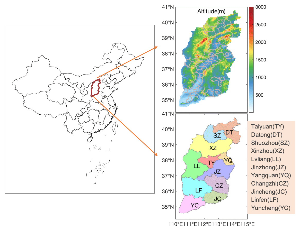
Figure 1Location, topography, and administrative division of Shanxi Province.
The sum of NO2 and nitric oxide (NO) is frequently grouped as nitrogen oxides (herein termed NOx), which is an important trace gas impacting Earth's atmosphere because it is a strong marker of anthropogenic combustion-related pollution, a precursor to ozone (Jacob et al., 1993), secondary aerosol (Rollins et al., 2012), and acid rain (Singh and Agrawal, 2008). In order to gain a better understanding of NOx and its impacts, precise and quantitative emission inventories are crucial information for policy makers, air quality modelers, climate change modelers, and those who conduct pollution weather response interactions, among others (Hoesly et al., 2018; Crippa et al., 2018; Li et al., 2017a; Xing et al., 2013; McDonald et al., 2013). However, it is challenging to quantify emissions in rapidly developing and changing areas accurately as there are a variety of contributing sources, a complex underlying mixture of combustion technologies, industrial restructuring, changing population dynamics, and ongoing atmospheric environmental management, all of which may lead to substantial changes in pollution sources.
Presently, most emission inventories are compiled from statistics representing emitting activities and associated typical emission factors, herein called “bottom-up” approaches (Ohara et al., 2007; Zheng et al., 2018; Li et al., 2017b). Bottom-up methods provide emissions data at finer scales. However, higher-resolution emission inventories using bottom-up methods require rich, detailed, and extremely precise records of energy use, facility locations, and other socioeconomic datasets from multiple regional and temporal scales (Cai et al., 2018), which frequently have a considerable amount of uncertainty (Bond et al., 2007). With the ever-increasing tightening of environmental management, emission factors have changed significantly and will continue to do so in the future. On-site surveys for bottom-up methods are time consuming and resource demanding. When performing laboratory emission factor determination, it is important to note that the differences among small field studies, controlled laboratory combustion experiments, and real-world examples also are quite significant, with super-emitters known to create large differences when using insufficiently large datasets (Zavala et al., 2006) and missing large sources leading to significant error (Wang et al., 2021). Due to the low temporal resolution and time-lag associated with many of these datasets, bottom-up inventories do not easily keep up with rapid changes in industry, economics, or pandemics, and they are therefore not very good at tracking atmospheric emissions under actual existing environmental conditions, limiting their use (Mijling and van der A, 2012).
To overcome the disadvantages identified above, while simultaneously improving the spatial and temporal resolution of emission inventories, attempts at top-down emission inventories using remotely sensed dataset have been made by the community. Some of these attempts have focused on applications to long-lived gases (CH4, CFCs, and N2O), since their chemical decay is slow compared with their transport processes, allowing a simpler set of approximations to perform the inversion (Chen and Prinn, 2006; Tu et al., 2022b; Liu et al., 2021). Satellite observations have also been widely used to quantify short-lived species such as NOx emissions (Martin, 2003; Beirle et al., 2019; Goldberg et al., 2019; Qu et al., 2019) by providing up-to-date and continuous time series of NO2 columns in different regions. Gaussian plumes have been used for a long time (Green et al., 1980), with more advanced but similar approximations including the exponentially modified Gaussian model to quantify the NOx emissions of isolated megacity sources (Beirle et al., 2011) and the probabilistic collocation method to train the emissions flux enhancement of megacities as a function of their size and shape (Cohen and Prinn, 2011). Some methods used a partial estimation of the mass balance approaches, including Beirle et al. (2019) and Kong et al. (2019). Another category based on atmospheric chemical transport models, climate models, and/or data assimilation, such as 3D-Var, 4D-Var, and Kalman filters, works very well but is susceptible to underlying model and scientific uncertainty, as well as being extremely computationally intensive (Cohen and Wang, 2014; Zhang et al., 2021). The selection of a priori inventories is crucial when using the methods above, since it has been demonstrated that missing sources frequently cannot be compensated for by merely scaling or increasing other existing sources if their spatial and temporal distributions are not matched correctly (Cohen, 2014). In recent years, continuous emission monitoring systems (CEMS) have been introduced in China, the USA, and other countries and areas as a means to monitor at the emissions effluent source in an integrated manner on an hourly and/or daily timescale, containing well-known aspects of quality control and assurance. This platform provides reliable technical information to fundamentally quantify local emissions on a stack-by-stack basis, in order to improve both the temporal resolution and magnitude of emission inventories (Tang et al., 2019; Gu et al., 2022; Chen et al., 2019; Lange et al., 2022).
This study takes advantage of the respective strengths of top-down and bottom-up emissions estimation by applying a new, fast, first-order approximation of physical, chemical, and thermal dynamics controlling the distribution of NOx in situ, and constrains these approximations using daily measurements of remotely sensed NO2 from the TROPOspheric Monitoring Instrument (TROPOMI) together with a mass-conserving inversion to estimate the daily NOx emissions on a mesoscale grid at () from January 2019 through December 2021. This approach partly originated from similar box-modeling ideas in previous studies (Rigby et al., 2008; Beirle et al., 2019; Kong et al., 2019), which themselves are based on a previous theory underlying the development of mass-conserving box models (Seigneur et al., 1986). In this specific work, the mass of emissions is connected with the in situ observed column loadings through application of the following factors: the temporal rate of change in column loadings, first-order chemical loss of NOx, gradient transport of NOx, and gradient transport of atmospheric air mass. The coefficients weighting these terms are flexibly fitted, allowing for a wider range of possible driving forces and solutions to be considered, while still requiring that these parameters are consistent with observations (Rollins et al., 2012; Karl et al., 2023). The fitted relationship is formed without the use of complex models, and can be run on a normal desktop computer, and the end product can be flexibly modified by the user for their own various applications. The a priori emissions used in this work come from daily CEMS observations at power plants and other large sources, as well as the Multi-resolution Emission Inventory for China (MEIC) over Shanxi Province. This unique approach is capable of using measured emissions, fitting variable parameters that were fixed in previous approaches, and inverting emissions as a function of their month-to-month constrained driving forces, under different but realistic environmental conditions. This method has been used in different situations such as over different months, over multi-year changes in the environment, under different actinic flux and atmospheric oxidation conditions, under complex meteorological domains, and over sources which are both thermodynamically stable as well as unstable. This allows this study to explore the full range of variations. Additionally, this approach allows for results with both robust error quantification and emissions that compare well with both the mean and the measured spatial and temporal variation in the underlying remotely sensed NO2 columns.
2.1 Tropospheric vertical column measurements from TROPOMI
TROPOMI measures reflected solar radiation in the UV, visible, and near-IR bands following a sun-synchronous, low-Earth orbit with an Equator overpass time of approximately 13:30 LT, allowing daily scale measurements across the globe (Veefkind et al., 2012; Goldberg et al., 2019; Tu et al., 2022a). In August 2019, the spatial resolution of TROPOMI was refined to 5.5 km × 3.5 km (Lange et al., 2022). This study uses two distinct products measured by TROPOMI over different radiative bands, but at the same place and time: NO2 and ultraviolet aerosol index (UVAI).
Daily level-2 version 2.3.1 tropospheric NO2 columns and version 2.2.0 UVAI over Shanxi Province have been introduced. All available days and swaths corresponding to the time period from January 2019 through December 2021 are analyzed (https://disc.gsfc.nasa.gov/datasets, last access: 28 June 2023). Overlapping NO2 and UVAI column pixels in each swath are resampled to a common latitude–longitude grid at using weighted polygons (http://stcorp.github.io/harp/doc/html/index.html, last access: 28 June 2023). Before use, it is required that all TROPOMI data are quality assured, specifically insisting that each pixel has a “qa_value” greater than 0.75, that the “cloud radiance fraction” is smaller than 0.5, and that scenes covered by snow/ice, errors, and similar problematic retrievals are removed (Henk et al., 2021). Furthermore, an additional filter is applied to set all individual grids of NO2 columns less than 1.4×10¹⁵ molec. cm−2 to be NaN. This is done to avoid issues where the observed signal may be smaller than the uncertainty of the signal itself (van Geffen et al., 2022; Qin et al., 2022). This combination of assumptions ensures that the data used will be of the highest possible precision based on the current available technology.
The average loadings, daily variation, and number of days without TROPOMI NO2 columns from 2019 through 2021 are shown in Fig. 2. The number of invalid days varies pixel-to-pixel from 357 to 742 d (521 d on average), with higher-altitude and mountainous areas tending to have more. The higher values on the maps are consistent with known urban and industrial regions, such as the Taiyuan, Xinding, and Linfen basins and Yangquan City. Areas with a high variation and a relatively low mean value are observed in regions where new economic development zones have been recently created or are in the process of being actively developed, including urban areas of Datong and Xinzhou. Areas with a relatively high variation and a high mean value are indicative of high urbanization and developed industrial areas, corresponding with the Taiyuan Basin and southern Yangquan. Areas with a high average value and a low variation correspond with regions that have fewer temporally consistent emission sources, as is observed in parts of the Linfen Basin, central Changzhi, Lvliang, and Jincheng, and industrial parks in the Jiexiu district of Jinzhong.
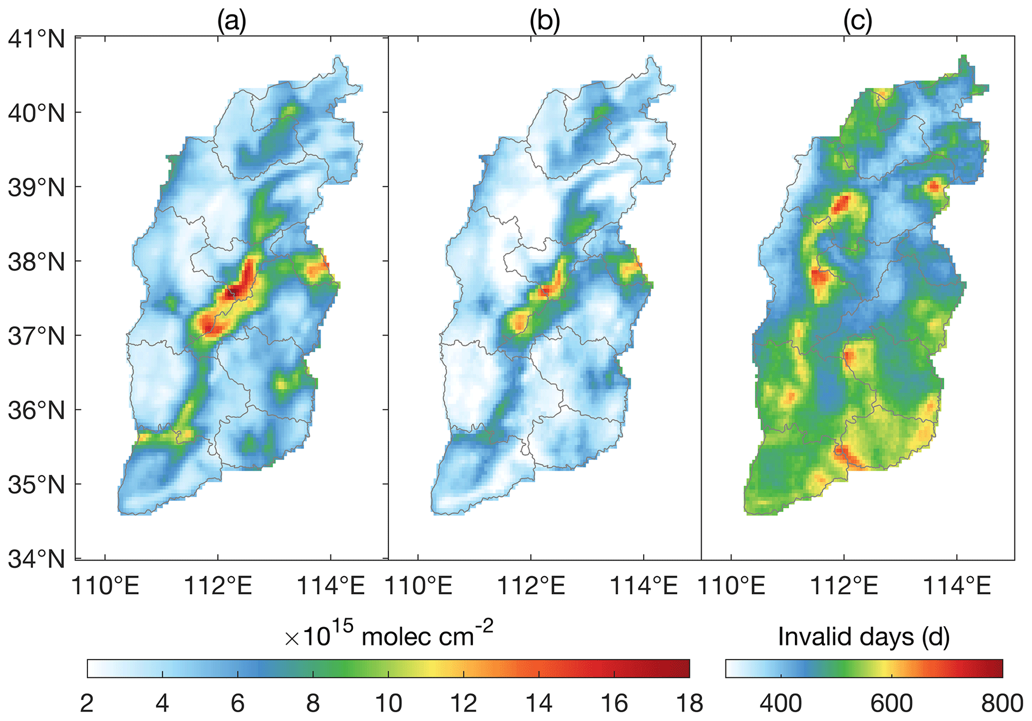
Figure 2TROPOMI daily NO2 column loadings from 2019 through 2021: (a) mean values (unit: molec. cm−2), (b) day-to-day standard deviation (unit: molec. cm−2), and (c) the number of invalid days (unit: d).
2.2 A priori emission inventories
2.2.1 CEMS
CEMS was introduced by the Ministry of Environmental Protection of China in 2007 to monitor and manage the emissions of certain (mainly high-emitting) plants (Schreifels et al., 2012; Karplus et al., 2018). CEMS makes actual stack flue gas measurements of the concentration of PM, SO2, and NOx as emitted from power plants, iron and steel plants, aluminum smelters, coke plants, coal-fired boilers, and others, all in real time (Tang et al., 2020; Zhang and Schreifels, 2011). Statistics of the emissions sites monitored in Shanxi are given in Table 1. There are two different technologies for measuring NOx concentrations. One converts NO2 to NO and measures the total NO concentration, the other measures NO2 and NO separately. Both of the measured results have been converted to NO2 mass concentration.
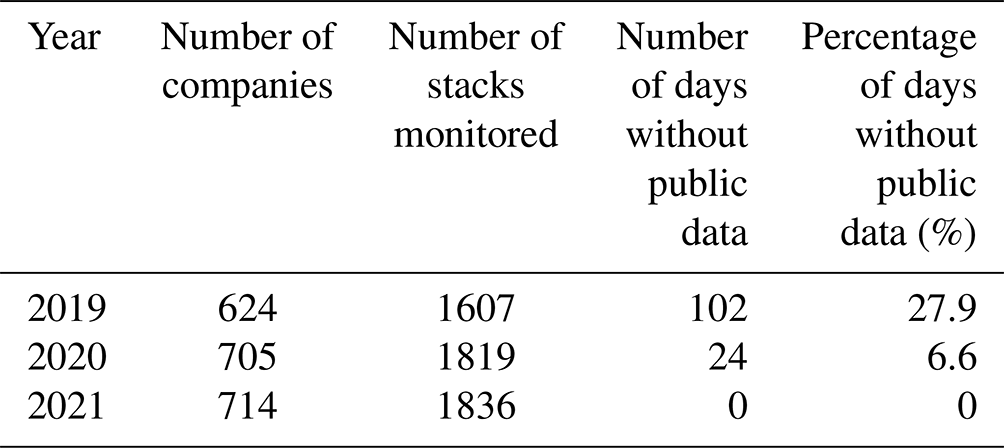
In this work, all available CEMS monitors of daily scale emissions from 2019 to 2021 were obtained from the Department of Ecology and Environment of Shanxi Province (DEESP), with the government taking great efforts to regulate the CEMS network and to ensure the reliability of CEMS data (Tang et al., 2020). Preprocessing of these data include using Google Earth to correct the location of the factories, conducting quality control on measured concentrations according to the CEMS technical requirements, including eliminating negative, outlier, and null values. The overall percentage of abnormal values is found to account for 0.63 %, 1.18 %, and 1.55 % of the raw data respectively for 2019, 2020, and 2021. The formula used to calculate NOx emissions is given in Eq. (1):
where is the daily average of hourly NOx concentration, mg m−3; is the daily average of hourly wet flue gas flow under actual working conditions, m3 h−1, and 24 is used to convert units from hours to days. Following the “Specifications and test procedures for a CEMS for SO2, NOx, and particulate matter in flue gas emitted from stationary sources (HJ/T76-2017)”, the uncertainty of NOx concentration (Ch) is less than or equal to 30 % for the data used in this study. After quality control, the emission intensity on a grid-by-grid basis is found to be 0.64±0.08, 0.45±0.13, and 0.41±0.05 µg m−2 s−1 for 2019, 2020, and 2021, respectively. Probability density functions (PDFs) of daily emission intensity and a map of the multi-year mean are displayed in Fig. 3. The largest number of low daily values occurred over a time period from one to two months in length (depending on the station) during the early part of 2020, which happens to be closely related to the pandemic, during which many key enterprises spontaneously shut down or otherwise limited production. However, on a year-to-year basis, the values in 2021 are lower than in 2020, reflecting the fact that the long-term efforts to reduce emissions may be even more important. Similarly, the highest emission intensity is observed in 2019.
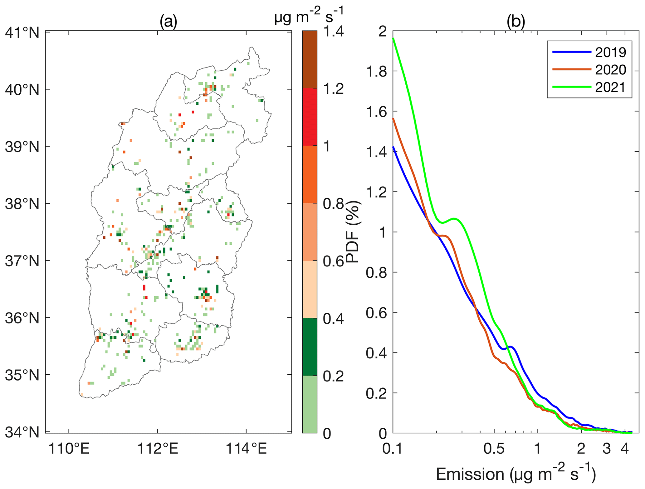
Figure 3CEMS emission intensity from January 2019 through December 2021 (unit: µg m−2 s−1): (a) 3-year average gridded NOx emissions, and (b) PDFs of day-to-day and grid-by-grid emissions over individual years (log-scale for x axis).
2.2.2 MEIC
At the present time, some of the emission inventories most widely used by the community are MEIC (Zheng et al., 2018) and the Emission Database for Global Atmospheric Research (EDGAR; Crippa et al., 2018). In this work, MEIC is selected since it provides bottom-up emissions of anthropogenic air pollutants over mainland China, with a monthly time step and a spatial resolution. NOx emissions are provided from January 2019 to December 2020 over five sectors: agriculture, industry, power, residential, and transportation (Zheng et al., 2021a). To match with the higher resolution of TROPOMI grids, all of the MEIC data in this work are mapped uniformly to a grid, with each TROPOMI-size grid assigned the same flux as the underlying MEIC grid. The average emission values and PDFs of the grid-by-grid data over Shanxi from 2019 January to 2020 December are given in Fig. 4a and b, demonstrating little change in emissions between the two years except for at very low values.
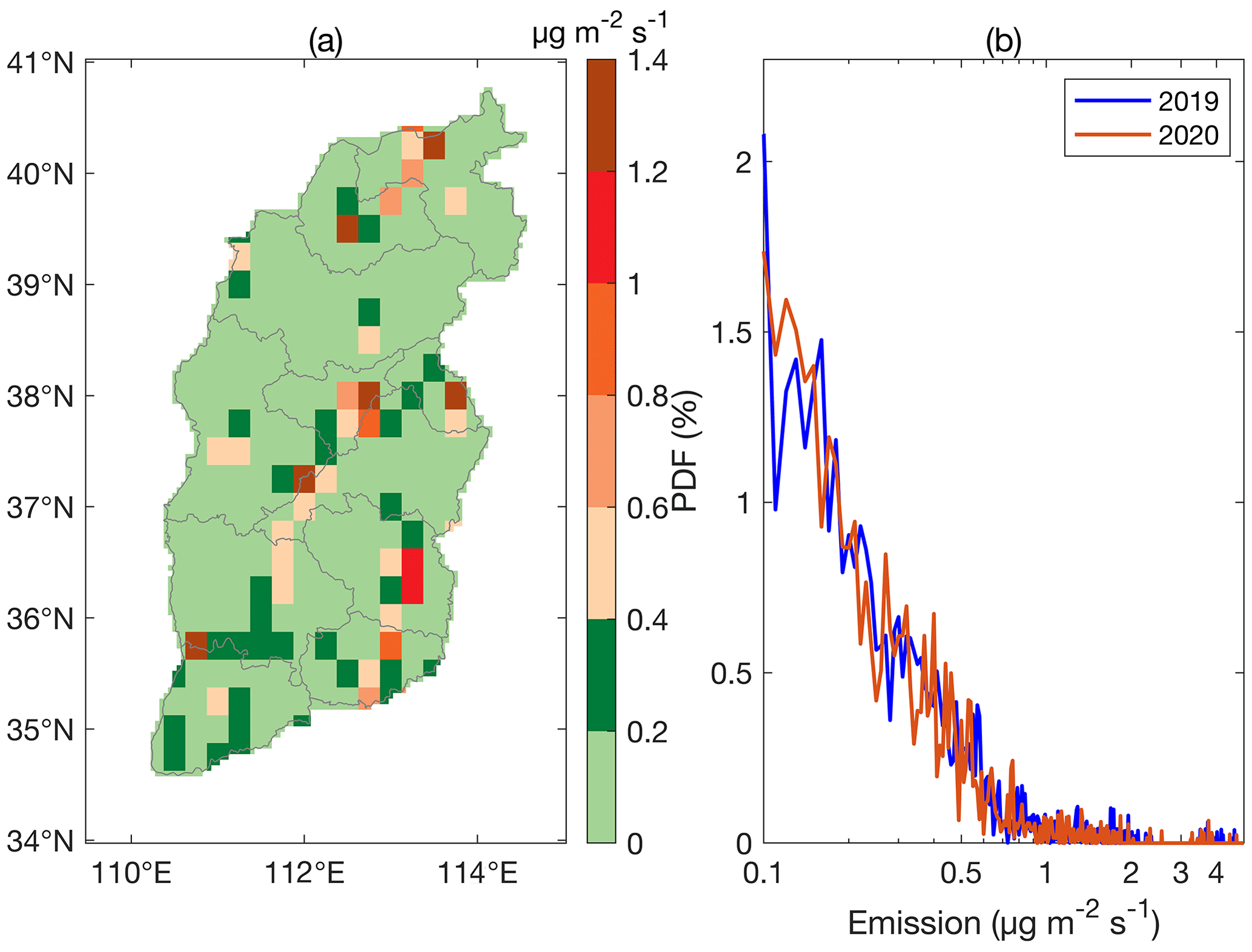
Figure 4MEIC emission intensity from January 2019 through December 2020 (unit: µg m−2 s−1): (a) 2-year average monthly MEIC emissions, and (b) PDFs of month-to-month and grid-by-grid emissions over individual years (log-scale for x axis).
2.3 Wind
Wind speed and direction are from the European Centre for Medium-Range Weather Forecasts (ECMWF) ERA-5 reanalysis products. This work uses the hourly 06:00 UTC u and v wind products (closest in terms of time to the TROPOMI overpass) at 850 hPa and resolution, available at https://www.ecmwf.int/en/forecasts/dataset/ecmwf-reanalysis-v5 (last access: 28 June 2023). The wind was linearly interpolated to follow the TROPOMI grid data in space. The reason for choosing the 850 hPa (which is approximately 1500 m) level is two-fold. First, Shanxi has complex topography, with less than 16 % of the total area of the province under 800 m in elevation, 68 % over 1000 m, and 17 % over 1500 m (see Fig. 1), leading to a significant amount of pollutant transport from near the ground to the lower free troposphere. Second, due to the relatively dry conditions, vertical plume-based rise is thought to be not insignificant (Wang et al., 2020). Overall, we aim to use wind speed and direction that correspond to a reasonable approximation of the median of the NOx emission vertical profile.
2.4 Variance maximization
To extract the spatial and temporal features of the extremes of the remotely sensed NO2 fields in an unbiased manner, the empirical orthogonal function (EOF) principal component analysis is applied. This technique decomposes the data into a set of orthogonal standing signals in space (EOF) and in time (PCA), with those signals contributing the most to the overall variance of the underlying dataset being selected, representing unique phenomenon that control the overall characteristics of the NO2 columns (Zhou et al., 2016; Lin et al., 2020). Further details, including mathematical derivations, are given in Björnsson and Venegas (1997) and Cohen (2014). This work retains the first three EOFs, which are found to contribute 43.3 %, 6.4 %, and 3.9 % of the total variation, with subsequent EOFs each contributing an insignificant amount (less than 3.9 %) and therefore no longer considered in this work (Greene et al., 2019).
2.5 Model-free inversion estimation framework (MFIEF)
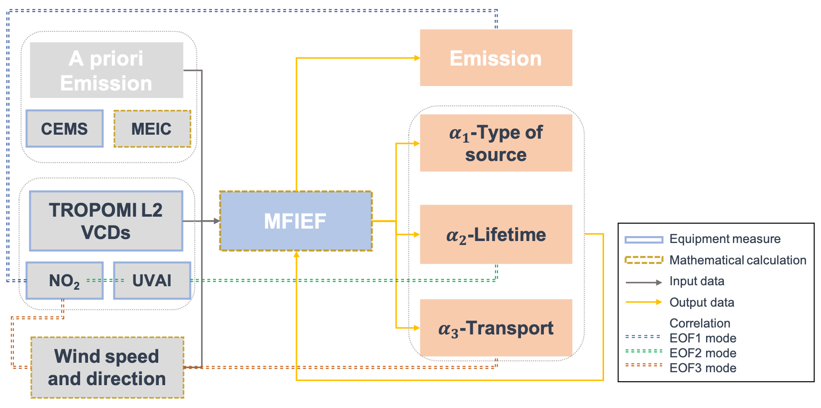
The MFIEF used here is based on a mass balance assumption Eq. (2), and the details are shown in Fig. 5. In the case where there is an observed change in the stock of NOx in the atmosphere, herein represented as C, in a Lagrangian sense, there must be either a source or a sink (Harte, 1988; Seinfeld and Pandis, 1997). When dealing with a fixed spatial grid, such as in this work, there is also a contribution of transport into or from the Lagrangian parcel. The first of these changes in the stock is due to the amount of NOx emitted, herein represented as E, which will always increase the existing stock. The second of these is the chemical loss of NOx, which will always lead to a decrease in the stock. The chemical sink of NOx is dominated by the reaction between NO2 and OH, via reactions with products formed from the actinic flux (i.e., chemistry such as RO2), and on aerosol surfaces via heterogeneous reactions (Valin et al., 2013; Kenagy et al., 2018; Romer Present et al., 2020), which herein is described as S. The third change in the stock is the sum of pressure-induced and advective transport, which may either increase or decrease the stock. The transport herein is described as D, and is calculated by the gradient of the product of the wind vector and the NOx column loadings, which consists of an advective portion (Wang et al., 2014) and a pressure-based portion (Mahowald et al., 2005). The mass conservation equation for NOx is calculated as
Solving Eq. (2) for emissions on a grid-by-grid basis requires knowledge of the mass change of the loading in time and space, and detailed consideration of chemical loss and transformation and of transport. An explicit formulation of these processes into a readily solvable mass balance method is derived as Eq. (3):
where represents the total atmospheric column emissions of NOx within the troposphere on a grid-by-grid and day-to-day basis in µg m−2 d−1. This is the total emission into each column accounting for all sources including anthropogenic sources (industry, vehicle, and residential), biomass burning, and others. represents the tropospheric NO2 column concentrations after it has been converted into µg m−2. Due to the fact that TROPOMI only measures NO2 rather than NOx, a transformation is required to transform NO2 columns into NOx, hereafter given as . , which computes the NOx concentration change rate in µg m−2 d−1, assuming the day-to-day temporal derivative of NO2 exists in the TROPOMI data on the respective days. represents the sink of NOx concentration, where α2 is related to the NOx lifetime (unit h), and 24 is the unit change factor. represents the gradients of daily zonal fluxes, meridional fluxes, and changes in the air column mass and density. These were derived by multiplying the gridded with the center point wind vector on a grid-by-grid basis in µg m−2 d−1. This computation assumes that the spatial gradient of TROPOMI NO2 and reanalysis wind both exist on the respective grids (Cohen and Prinn, 2011). In this case, α3 is the parameter representing the transport distance (in kilometers) per day, where 0.001 is used to convert meters to kilometers. is observed as either one or two overlapping snapshots of total column information occurring at 13:30 LT (and under some conditions also 101.5 min either earlier or later; Tonion and Pirotti, 2022). In all cases, the meteorological values and CEMS values are representative of 24 h total and/or daily average conditions, respectively. Therefore, the fitted values of α1, α2, and α3, as presented, are representative of either a 24 h average or 24 h net effect, acting on the entire column of NOx. In all cases, the values of α1, α2, and α3 are computed month-to-month over all grids in which data are available, and by bootstrapping at other grids and times.
2.6 Additional analytical methods
This work employs multiple linear regression to fit the values of α1, α2, and α3 on a month-to-month and grid-by-grid basis using all available daily measurements and Eq. (3). These values are further filtered based on both statistics (p<0.15 and removal of outliers defined as elements that are more than three scaled median absolute deviations (MADs), calculated by Eq. (4)) and being physically realistic (, α2<0).
α1, α2, and α3 are brought into α in Eq. (4) respectively for outlier rejection. Bootstrapping is used as a means to create a new sample to represent the parent sample distribution through multiple repetitions of sampling (Liu and Cohen, 2022). Specifically, the distributions of α1, α2, and α3 are sampled across the central 80 % of their probability distributions, which are then used to generate a set of pseudo α1, α2, and α3 on a grid-by-grid basis where there is no existing a priori and therefore no actual solution of these variables. These bootstrapped pseudo α1, α2, and α3 are then used on these specific grids to approximate the emissions of NOx using Eq. (3) on a daily basis where TROPOMI NO2 column data and wind data are available. The mean data have been taken out as the daily emission, while the standard deviation was calculated as the uncertainty of the daily emission.
3.1 Computed emissions using CEMS and MEIC
Figure 6a and b show the spatial distribution of the daily average and variation of NOx emissions based on CEMS (EICEMS) from January 2019 to December 2021 over Shanxi at . For all subsequent emission values displayed, the numbers correspond to the sum over the day-to-day mean ± uncertainty. It is observed that the grids with the highest NOx emissions in Shanxi are mainly concentrated in the lower Fen River valley. This also happens to be located at the lowest-altitude areas in the province as shown by area marked by a pink line in Fig. 1, containing the Taiyuan, Xinding, and Linfen basins, which also corresponds to the area containing the highest population density. This area in total accounts for around 25 % of the total area of the province and contributes 53 % (0.98±0.55 Tg yr−1) of the total NOx emissions (1.86±1.05 Tg yr−1) in Shanxi. It is of significance to note the regions with a moderate average density of emissions, ranging from 0.3 to 0.7 µg m−2 s−1, contribute 62 % (1.15±0.64 Tg yr−1) of the total emissions. The use of MFIEF can effectively optimize the distribution of the inventory and perform inventory correction based on satellite data, while complementing many areas where there is no existing emissions data, incomplete data, mischaracterized data, or data which may be reasonable on average but not account for daily scale variability.
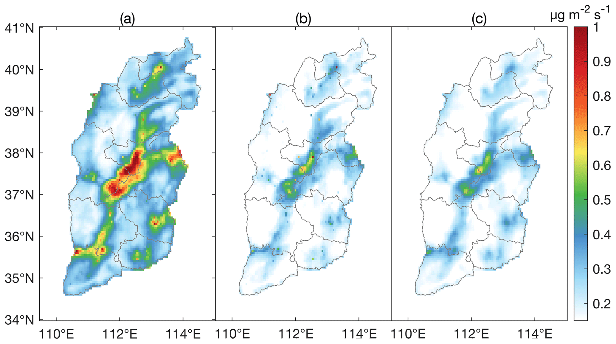
Figure 6Daily average emissions based on CEMS from January 2019 to December 2021 over Shanxi at (unit: µg m−2 s−1): (a) daily average NOx emissions. (b) Day-to-day variability of NOx emissions. (c) Bootstrapping uncertainty range (10 % to 90 % of distribution).
MEIC was also separately used as the a priori with MFIEF to produce an additional emissions inventory from January 2019 to December 2020, herein called EIMEIC. The total EIMEIC over the province is 1.34±0.60 Tg yr−1. The multi-annual mean value of EICEMS minus EIMEIC and histogram of the day-to-day and grid-by-grid emissions of both EICEMS and EIMEIC from 2019 to 2020 are displayed in Fig. 7. On a multi-annual average basis, EICEMS is larger than EIMEIC at 98 % of grids, while on a day-to-day basis it is larger at 90 % of grids. Some higher value appeared in EIMEIC calculated by high MEIC values in some places of Shuozhou, Yangquan, Lvliang, Changzhi, and Jincheng may be due to mispositioned hotspots in the existing inventories, in terms of both space and time. Conversely, EICEMS better captured residential and small industrial sources than EIMEIC. This is possibly due to the fact that the a priori MEIC distribution has many low values which actually fall within the uncertainty of the bottom-up emissions processes (Cohen and Wang, 2014; Bond, 2004; Crippa et al., 2018). The low a priori emissions on a grid-by-grid basis in turn shift the physically filtered values of α1 towards lower values. At the same time, the values of α2 were shifted to higher values. In tandem with these, the transport term α3 was shifted to include larger absolute values of distance. This net combination caused the final calculation to be less biased overall.
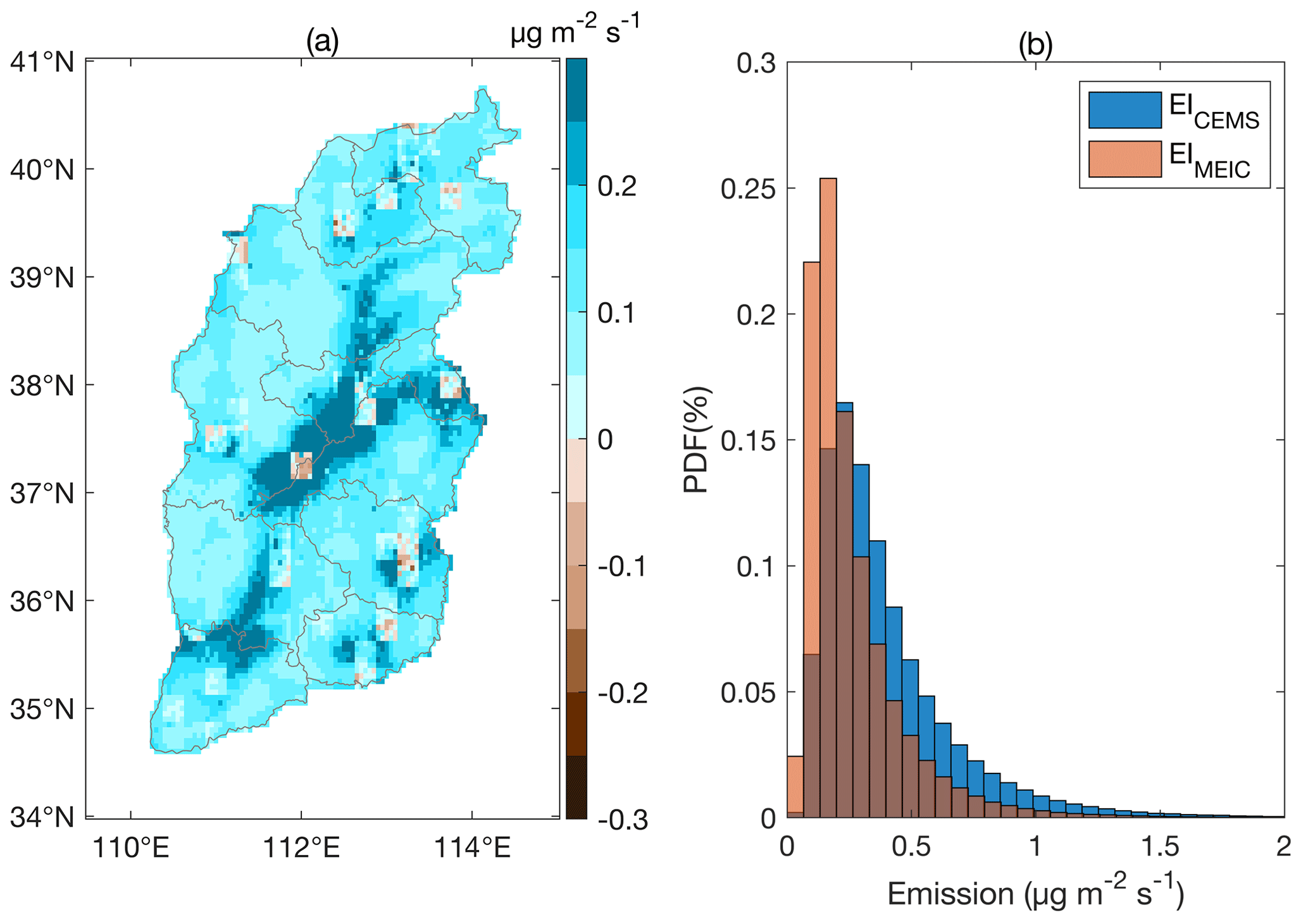
Figure 7Differences between EICEMS and EIMEIC from 2019 to 2020 (unit: µg m−2 s−1): (a) average values in space of EICEMS minus EIMEIC. (b) Histogram of EICEMS and EIMEIC.
Figure 8 shows the differences between CEMS, EICEMS, EIMEIC, and MEIC, as well as the 30 % error range for CEMS and the computed 10th to 90th percentile error ranges for EICEMS and EIMEIC as computed from January 2019 to December 2020 in all 11 cities in Shanxi. It shows that while generally CEMS is larger than EICEMS, that they are always found to be within the error ranges of each other, while EIMEIC only overlaps with CEMS in six cities. Similarly, MEIC is always found to be the lowest, while EIMEIC is found to be larger than MEIC and smaller than EICEMS. In particular, EICEMS and EIMEIC have error ranges which overlap in all cities, while MEIC overlaps with the EIMEIC range in eight cities.
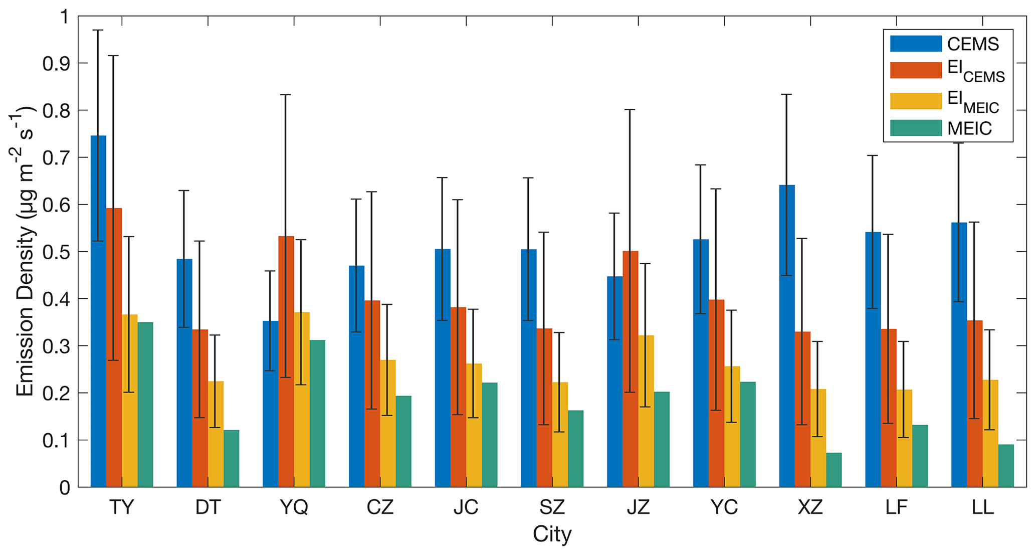
Figure 8Differences between CEMS, EICEMS, EIMEIC, and MEIC with their error ranges from 2019 to 2020 in all 11 cities in Shanxi (unit: µg m−2 s−1).
3.2 Underlying factors contributing to variance maximized TROPOMI NO2 columns
A deeper analysis of the factors contributing to the variance in the TROPOMI NO2 column measurements is essential to determine if the computed emissions and underlying factors are consistent with the remotely sensed fields both in terms of mean value and temporal variability. Recent practice has devised a way to ensure this consistency through the use of an EOF Analysis (Cohen et al., 2017; Cohen, 2014; Lin et al., 2020), which is applied to the daily TROPOMI NO2 columns. The three spatial modes contributing the most variation to the observed daily TROPOMI NO2 fields (EOF1, EOF2, and EOF3) contribute 43.3 %, 6.4 %, and 3.9 % respectively, as shown in Fig. 9.
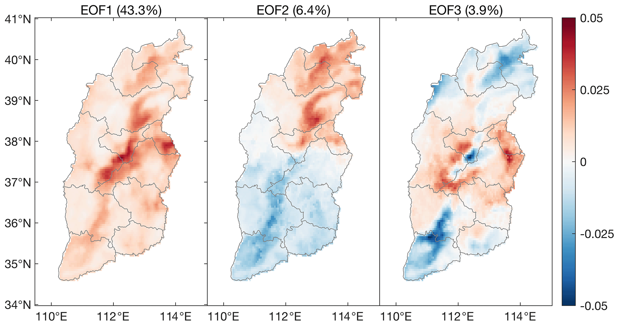
Figure 9Spatial distribution map of first three modes (a) EOF1, (b) EOF2, and (c) EOF3.
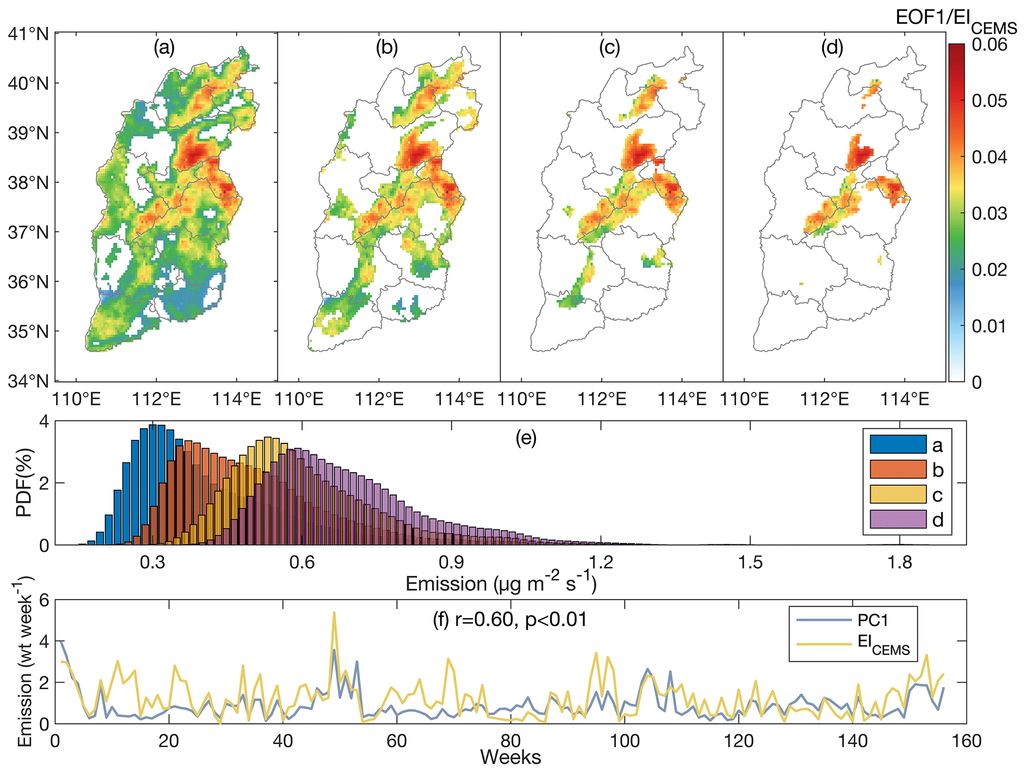
Figure 10Four different cutoffs of EOF1 are used to set the different spatial domains. The maps in (a)–(d) are plots of EOF1/EICEMS where the cutoffs are given as (a) EOF1 > 0.005, (b) EOF1 > 0.01, (c) EOF1 > 0.015, and (d) EOF1 > 0.02. (e) Histogram of the EICEMS over the domains given respectively in (a)–(d). (f) Time series of weekly PC1 compared with EICEMS over the whole domain.
It is asserted that EOF1 is directly driven by EICEMS. The comparison of EOF1 and the emissions is shown in Fig. 10 in terms of both spatial and temporal scales. By applying four different progressively increasing cutoffs to the domain of EOF1, it is observed that as the EOF1 domain increases in magnitude, the 3-year mean EICEMS computed over the same domains also increase in magnitude. Therefore, the more extreme the EOF1 value, the higher the emissions, demonstrating that the emissions are responsible for the first mode of the maximized variance. EICEMS is also found to statistically correlate with PC1 (r=0.60, p<0.01), indicating that the first mode of variation is strongly connected with the changes in EICEMS in terms of both spatial and temporal dimensions.
Second, it is asserted that EOF2 is related to TROPOMI-measured UVAI, which physically makes sense, since satellite observations of UVAI are sensitive to aerosol extinction in the UV, with very large values indicating large amounts of highly absorbing aerosol (single-scattering albedo, SSA, less than 0.9) and very large negative values indicating large amounts of partially absorbing aerosol (SSA between 0.92 and 0.98; Penning de Vries et al., 2009; Torres et al., 2020). There have been numerous studies reporting that absorbing aerosols affect the downwelling surface radiative forcing in the visible (and therefore the actinic flux; Léon, 2002) as well as OH concentrations (Hammer et al., 2016). Therefore, UVAI is an indirect proxy of an aspect contributing to the chemical decay capacity of NOx in situ. Applying four different cutoffs to EOF2, it is observed that as the EOF2 domain increases in magnitude, the 3-year mean measured absolute value of TROPOMI UVAI becomes smaller in magnitude, as demonstrated in Fig. 11. Since values of UVAI closer to zero imply less atmospheric extinction (absorption for positive values and a mixture of scattering and absorption for negative values), it therefore also scales inversely with surface UV radiation, implying that when the UVAI is lower, there is more available UV radiation, and hence implicitly faster chemical decay of NOx. This is consistent with the UV radiation being responsible for the second mode of the maximized variance. The negative correlation observed between absolute values of UVAI weighted by high absolute values of EOF2 (EOF2 > 0.02) grid-by-grid in the same EOF2 region is anticorrelated with PC2 (, p<0.01). While r in this case is much smaller, it is also consistent with theory, since in order to significantly affect the OH levels, the changes in UV radiation and hence UVAI must be very large, which is found to not occur frequently in time, but when it does occur, it makes a significant impact.
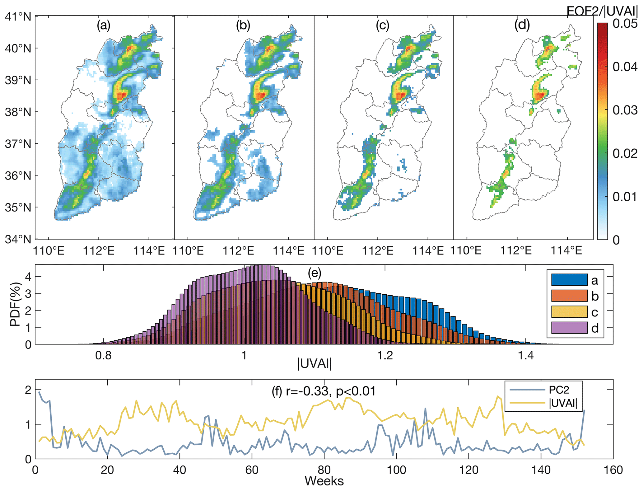
Figure 11Four different cutoffs of EOF2 are used to set the different spatial domains. The maps in (a)–(d) are plots of EOF2/|UVAI| where the cutoffs are given as (a) EOF2 > 0.005, (b) EOF2 > 0.01, (c) EOF2 > 0.015, and (d) EOF2 > 0.02. (e) Histogram of |UVAI| over the domains given respectively in (a)–(d). (f) Time series of weekly PC2 and |UVAI| in the (d) domain.
Finally, it is asserted that EOF3 is related to the transport of NO2. This term has been specifically computed by taking the variance of the multiple of wind and TROPOMI NO2 column loadings, specifically ). Similarly to the above cases, it is demonstrated that in the case where four different cutoffs are applied to EOF3, as the EOF3 domain increases in magnitude, the measured transport based on TROPOMI NO2 also increases, as seen in Fig. 12. ) weighted by EOF3 grid-by-grid positively correlates with PC3 (r=0.74, p<0.01), indicating that the third mode of variability, PC3 is strongly consistent with ) in the temporal dimensions. Therefore, transport is responsible for the third mode of the maximized variance.
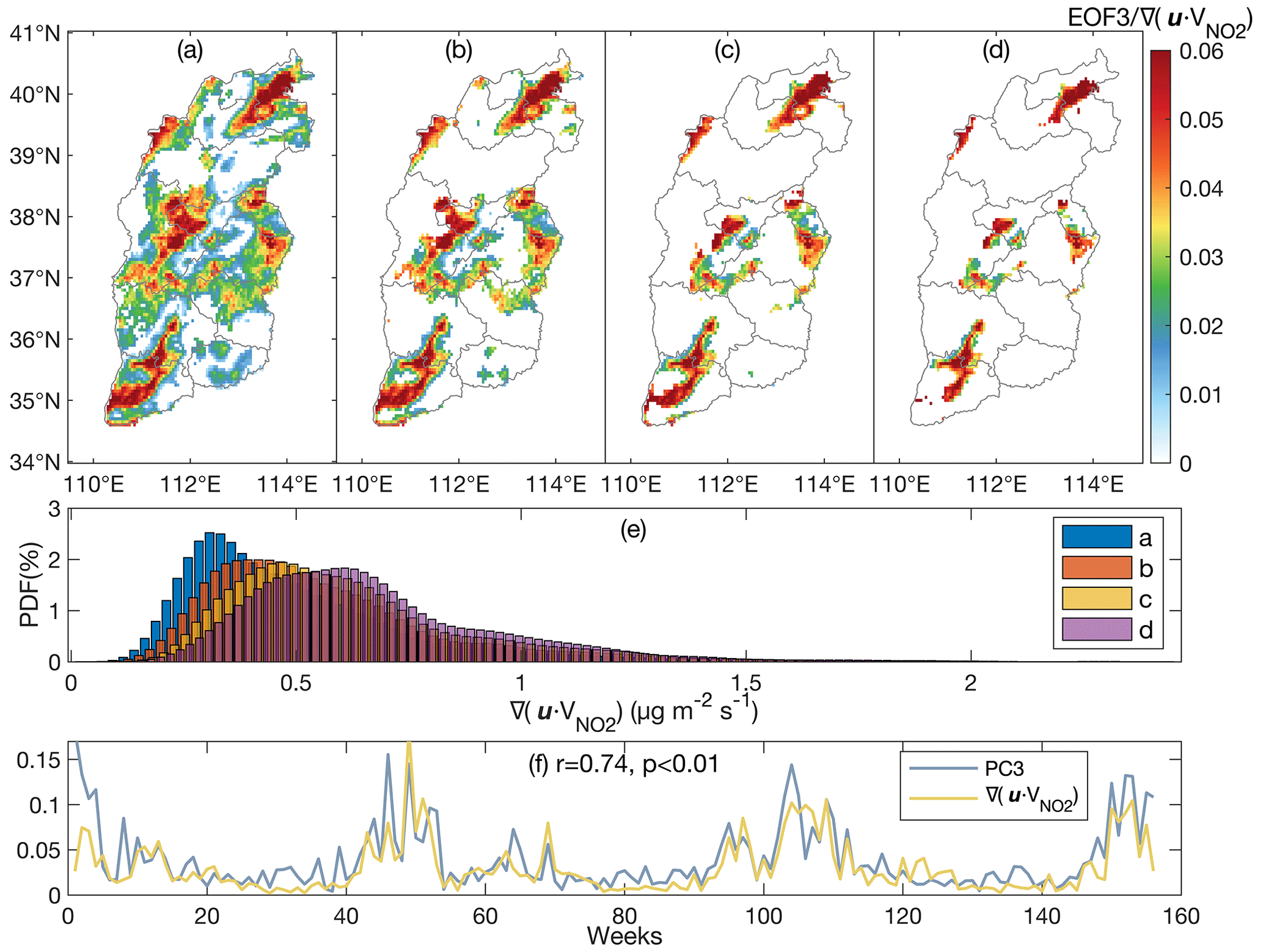
Figure 12Four different cutoffs of EOF3 are used to set the different spatial domains. The maps in (a)–(d) are plots of EOF3/NO2 transport where the cutoffs are given as (a) EOF3 > 0.005, (b) EOF3 > 0.01, (c) EOF3 > 0.015, and (d) EOF3 > 0.02. (e) Histogram of the NO2 transport over the domains given respectively in (a)–(d). (f) Time series of weekly PC3 compared against over the whole domain.
3.3 Uncertainty in emission and the parameters
The uncertainty of the computed emissions on a grid-by-grid and day-to-day basis is due to a combination of uncertainties in the satellite data, CEMS or MEIC as a priori emissions, and the calculations involved with computing the various best-fit parameters. NOx column concentrations and CEMS both have uncertainties of about 30 %. Another uncertainty comes from the parameters α1, α2, and α3 generated during the regression of Eq. (3) as given in Sect. 2.5. The fitted coefficients are computed month-to-month over the 3 years from January 2019 through December of 2021. Their absolute value overall mean, 10th percentile, and 90th percentile are found to be , h, and km. However, it is observed in the fits that some amount of the variability is not uniform in space and time, with the month-to-month values and standard deviations given in Fig. 13. In general, α1 tends to be slightly higher during one or a combination of both hotter months and times when the UVAI is low (hence the UV values are high). α2 over the lifetime reflects all hours of the day; in general, it tends to be variable: both interannual and intra-annual variations seem to drive most of the change. Given that this is related to both the column-average temperature and UV availability, the largest values are found in June or July and the lowest values are found in September. Furthermore, there are other complex forcing factors such as the height of the aerosol layer, the total aerosol loadings, and cloudiness, among other factors. The absolute magnitudes of α2 and their uncertainty ranges are reasonable when compared with vertically integrated and 24 h integrated chemical transport model values. In general, α3 also seems to not have any significant seasonal or monthly pattern, with interannual and intra-annual terms seeming to dominate. The values tend to be slightly larger than chemical transport models account for, but are reasonable when compared with the ultra-long-range transport simulated for plumes that break the boundary layer. This range, combined with the wide basins of 200 to 400 km in length, seem to provide a reasonable bound on the output results. One possible reason for this is that the atmospheric wind patterns were slightly different in 2019 due to the El Niño pattern (Hu et al., 2020). The result of overall uncertainty of the emissions as a result of the overall bootstrapped fitting ranges from 32 % to 70 % on a grid-by-grid basis, as shown in Fig. 6c. In general, the larger relative uncertainty values are observed over mountain regions. A sensitivity test has been performed to test the robustness of the fits assuming that the TROPOMI NO2 column values are varied near the extreme top and bottom of their 30 % uncertainty range. It is shown that the new NOx emissions in the 70 % case are always larger than 0.7 times the original emissions case (spatially annually averaged and grid-by-grid, varying from 0.89 to 1.00; temporally domain averaged, varying from 0.77 to 1.04). Similarly, the new NOx emissions in the 130 % case over the median 90 % of data is smaller than 1.3 times the original emissions case (spatially annually averaged and grid-by-grid, varying from 1.08 to 1.12; temporally domain averaged, varying from 1.01 to 1.30).
3.4 Application of α1 to analyze different combustion technologies
A significant finding is observed when the value of α1 is analyzed more closely on a pixel-to-pixel level and compared with underlying CEMS combustion source types. This analysis is motivated by the fact that NOx is produced during high temperature combustion of air, with three different major parts contributing to the overall amount of NOx produced: thermal NOx formation, fuel NOx formation, and chemical NOx formation (Schwerdt, 2006; Le Bris et al., 2007). Thermal NOx formation describes the process when N2 reacts with O2 in the air at high temperatures (Le Bris et al., 2007), with NO2 forming preferentially at temperatures between 800 and 1200∘ and NO forming preferentially at temperatures above 1200∘. Thermal NOx usually dominates the overall NOx production when the temperature is over 1100∘, and reaches a maximum contribution when the temperature is over 1600∘. There is additional NOx produced due to free nitrogen in the fuel itself. Finally, chemical decay may occur when there are mixed organo-nitrides, resulting in the prompt NOx formation. Therefore, a deeper understanding of the overall and oxygen partial pressures and temperature in the combustion chamber are all important for NOx formation. In summary, as the temperature of combustion increases, both the amount of NO and NO2 will increase. When the temperature exceeds 1200∘, NO will continue to increase while NO2 will decrease. During any time when the pressure increases, the yield of NO2 will also decrease and NO will increase (Aho et al., 1995; Turns, 1995).
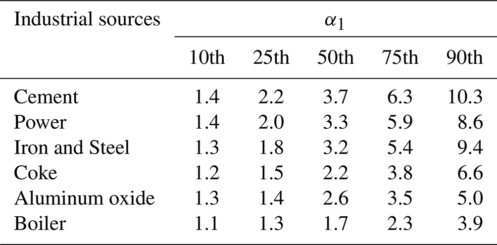
A deeper look at the various different CEMS sources (cement, power, iron and steel, coke, boilers, and aluminum oxide) reveals that the internal combustion processes are extremely important in terms of the overall value of α1. The statistical distribution of α1 and the calculated values of α1 at the 10th, 25th, 50th, 75th, and 90th percentile values (given in the Table 2) clearly demonstrated that cement factories have the highest value, power and iron and steel have the next highest values, coke and aluminum oxide are significantly lower still, and boilers have the lowest values. Further details are also clearly observed. For example, power and iron and steel have significant differences across different parts of the distribution with power having larger values from the 25th through 75th percentile range and iron and steel having a higher value at the 90th percentile level. This is consistent with the fact that iron and steel use several different processes, one of which contains very high temperature combustion (blast furnace based) and another which contains a lower temperature process (sinter bed based). Other differences are explained more in depth herein.
Table 2Distribution of α1 at the corresponding 10th, 25th, 50th, 75th, and 90th percentile values using MFIEF at different industrial sources where CEMS has observations.
Production of cement is a major source of NOx in Shanxi, with the major technology being dry process rotary kiln technology. Given that the temperature of the main burner of cement rotary kilns are higher than 1400∘, with some peaking as high as 1800 to 2000∘ (Wu et al., 2020; Akgun, 2003), it is expected that there will be a large amount of thermodynamic NOx generation. As observed at the cement CEMS sites, the computed α1 has a value always within or above the values computed at power plants, including both in terms of the mode and at the highest emitting individual values, as show in Table 2 and Fig. 14. Iron and steel are produced through a set of different processes, involving combustion at a range of different temperatures. The steps involved in the blast furnaces and some other processes require a high flame temperature, in the range from 1350 to 2000∘. There are further processes occurring that require a relatively lower temperature, such as in the sinter bed stage, where the highest temperature is only about 1300∘ (Zhou et al., 2018). Therefore, while in general the values are relatively high compared to the other source types below, and are generally found within the range of values at power plants, there are some individual differences as well, including a larger fraction of large values (9–10) and a smaller fraction at very large values (15–17), as observed in Fig. 14. The maximum temperature of the combustion chamber of thermal power plants can reach 2000∘. In fact, such plants are constantly finding ways to increase combustion efficiency so that they can be more energy efficient and produce as much energy per ton of CO2 emitted. α1 is relatively high at these sites, consistent with thermal production.
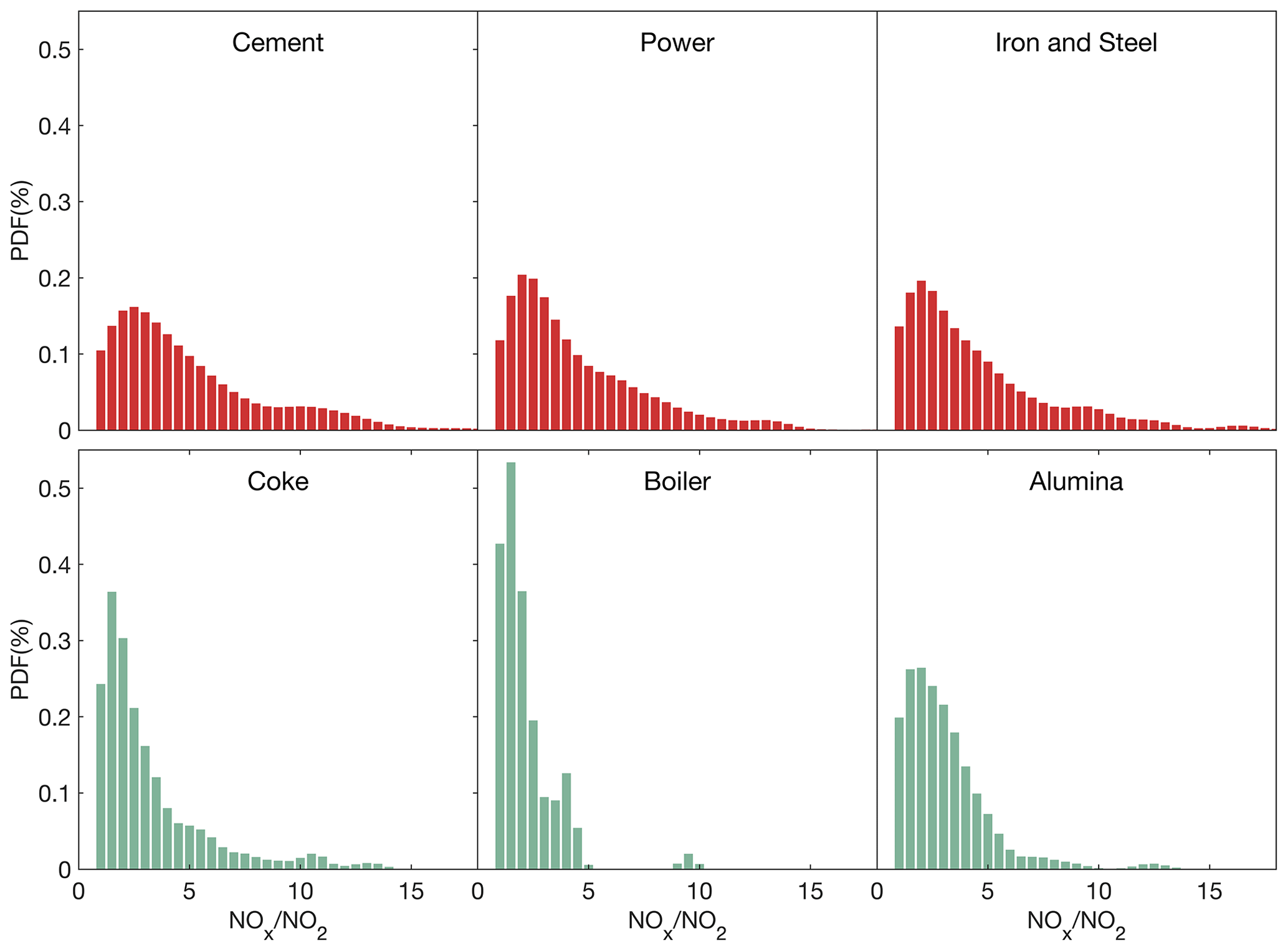
Figure 14Histograms of monthly α1 calculated using MFIEF at the following sources where CEMS has data: cement factories, power plants, iron and steel factories, coke ovens, boilers, and aluminum oxide factories.
Boilers use a similar technology as power plants, but tend to be smaller and run at a lower temperature range and efficiency. This is because their use is to produce hot water and steam for direct residential and industrial use, not high-pressure steam to run turbines. In general, these boilers have a much smaller overall capacity; therefore, without access to CEMS, they may not be otherwise be detectable. For these reasons, it is logical that there is a greater amount of NO2 produced than the above cases, and subsequently the value of α1 is much lower, in terms of both the mode and all moderate values (5 and larger), as shown in Table 2 and Fig. 14. Coke and aluminum oxide are both produced using a different technique from the other combustion sources, specifically focusing on creating high temperature, oven-like conditions to bake/roast their products. The average temperatures of coke ovens charring chamber and aluminum oxide roasting furnaces are around 1000 ∘C (Abyzov, 2019; Neto et al., 2021), with the material temperature continuously held at that temperature for a long period of time, e.g., 1 d. At the same time, the oxygen content is low. In total, there is far less thermal NO and more thermal NO2. Aluminum is also smelted in oven-like conditions. Correspondingly, while the mode of α1 for aluminum oxide is more similar to iron and steel, and the mode of α1 for coke is slightly lower, their distributions over the range are quite different from each other. Iron and steel is consistently higher than the other two from the 25th percentile and upwards, aluminum is higher than coke from the 50th percentile and lower, and coke is higher than aluminum from the 75th percentile and higher. All of the species have distributions in which the bulk of their distribution are skewed lower, while simultaneously exhibiting a small but not insignificant tail, as detailed in Fig. 14.
In addition, in situ processes also impact the value of α1 since there is a rapid adjustment after emitted from a combustion stack into the atmosphere, before the parcel comes to thermodynamic equilibrium (Cohen et al., 2018; Wang et al., 2020). From Fig. 13a it can be seen while there is a pattern where the values are higher in certain months than others, there is also a clear difference between the different source types. This demonstrates clearly that atmospheric processing modulates the process to some extent but does not dominate the signal on average. This is especially important in the case of hotter power sources, since they will contain more buoyancy, and rise to a greater height, making them more likely to be in contact with air which is more exposed to UV and also generally colder than the surface. Overall, the value of α1 seems to rely on both the temperature under which the initial NOx was generated, as well as any rapid processes taking place once it is emitted into the atmosphere (including photo-chemistry and vertical lofting).
MFIEF based on daily measurements from TROPOMI and a priori daily emissions from CEMS successfully inverts daily NOx emissions. First, the emissions computed match well with known urban, suburban, and industrial locations. Secondly, the best fit values for thermodynamics (α1) and first-order chemical decay (α2) are both physically realistic, while the best fit term for transport (α3) is reasonable based on the mountain and basin geography of the province. Thirdly, the variability of emissions in terms of different geographic location, source types, special events which changed the emissions levels (such as the onset of COVID-19), and general oxidative, photochemical, and transport conditions of the atmosphere on a monthly scale are all consistent with what is known. Fourth, the uncertainty is observed to be lower than the day-to-day variability over 30 % of the region and is mostly distributed in regions with higher emission intensities, showing that the results on a day-to-day basis are significant.
MFIEF emissions computed using different a priori datasets (CEMS versus MEIC) yield significant differences from on-the-ground CEMS measurements and local geospatial knowledge of where large sources exist. EIMEIC severely underestimates sources which have a lower amount of emissions, as well as newer sources, while at the same time overestimates sources in Yangquan, Xiaoyi, and enormous steel and power plants, among other similar high emissions sources. EIMEIC incorporates too many low values from MEIC in the suburban and rural areas, leading to many of these grids possessing physically unreasonable or at best very low/high values. A site-by-site comparison with CEMS shows very large differences with EIMEIC at locations which MEIC does have an a priori value, indicating that any a priori dataset must be both precise and accurate, including on a day-to-day basis in order to present a good overall model fit and emissions output product. The MFIEF method as a procedure can quantitatively allay some of these shortcomings of present-day a priori inventories.
The results of variance maximization analysis of 3 years of daily TROPOMI NO2 columns reveal three patterns that drive the variability in the NO2 columns. EICEMS is attributed as responsible for pattern 1, measured UVAI from TROPOMI (which is inversely related to photochemistry) is attributed as responsible for pattern 2, while transport (computed from the gradient of reanalysis wind and TROPOMI NO2 columns) is attributed as responsible for pattern 3. This procedure and its results form a basis of a best-practice approach that the community can adapt to subsequently analyze the efficacy of future emissions products. It is essential to ensure that emissions not only match on average but also match well with the observed spatial and temporal gradients of the observed remotely sensed fields.
It is observed that the calculated values of α1 are correlated with the thermodynamic conditions of underlying large combustion sources. This offers a new and self-consistent way to quantify the underlying combustion conditions of NOx generation using remotely sensed measurements. The highest mode and very high values are consistently associated with α1 at cement factories. Generally, high modes of α1, with significance at moderately high and high values, are found respectively at iron and steel and power plants. Locations that have CEMS aluminum oxide plants, coke ovens, and boilers are generally lower, but in the case of both aluminum oxide and coke ovens, there is still a significant range of α1 up to 5, while in the case of boilers, there is nearly no high value. There is a slight offset based on the atmospheric temperature, UV radiation, and other atmospheric mixing and chemical forcings, with both colder and lower radiation months having α1 slightly negatively offset and hotter temperature and higher radiation conditions having α1 slightly positively offset. While this offset is consistent across all plant types, it is slightly stronger for the hottest types (cement, iron and steel, and electricity), which are most likely to rise to a higher elevation and therefore be more impacted by the surrounding atmospheric conditions. In all cases, this offset is smaller than the difference between the different source types, indicating that attribution is possible.
The procedure introduced here offers a next step advance in terms of computing emissions from a top-down perspective. Community adaptation and use of these new results will ideally allow improvement in bottom-up inventory constraints and attribution. This work would be improved by reduction in remotely sensed measurement errors/uncertainties, increased use of and access to surface CEMS and other high-quality surface flux measurements, improved a priori emission databases, and higher-frequency temporal data availability from new geostationary satellite platforms. The adaptation of day-to-day and other higher-frequency quantification data sources, especially sources with well-quantified errors would also improve the work herein. The ability to identify large and moderately large industrial sources could be used to identify and quantify sources from many parts of the Global South where ground-based measurements may not be readily available. It is hoped that the findings herein will be improved upon, possibly in an iterative manner, allowing for more precision and predictability, so that emissions and environmental regulators can have more quantitative support to focus their efforts.
The satellite NO2 datasets used in this study are available at https://disc.gsfc.nasa.gov/datasets/S5P_L2__NO2____HiR_2/summary?keywords=tropomi NO2 (GES DISC, 2022). The ERA-5 reanalysis product is available at https://doi.org/10.24381/cds.bd0915c6 (ECMWF, 2022). The CEMS on-line data are available at https://sthjt.shanxi.gov.cn/wryjg/jczf (DEESP, 2017). The MEIC product can be accessed from https://doi.org/10.6084/m9.figshare.c.5214920.v2 (Zheng et al., 2021b). All of the data and underlying figures are available for download at https://doi.org/10.6084/m9.figshare.20459889 (Li et al., 2023).
XL, JBC, KQ, and HG developed the research question and set up the whole experimental program. XL wrote the manuscript and performed the data analysis with input from JBC, KQ, RZ, LW, and LZ. LW compared this result with the existing emission inventories and environmental statistics data. LW and XW rectified the deviation of the CEMS location and made statistics of annual changes. JBC drafted and corrected the manuscript. HG, XW, CY, RZ, and LZ consulted on the local situation and CEMS data. All authors discussed the results and contributed to the final manuscript.
The contact author has declared that none of the authors has any competing interests.
Publisher's note: Copernicus Publications remains neutral with regard to jurisdictional claims in published maps and institutional affiliations.
The authors would like to thank CEMS for the provision of their emission data. The authors also thank the PIs of the TROPOMI, ERA-5, and MEIC products for making their data available. The study was supported by the National Natural Science Foundation of China (42075147 and 41975041), the Shanxi Province Major Science and Technique Program (202101090301013), the Fundamental Research Funds for the Central Universities (2023KYJD1003), and the Shanxi Province Postgraduate Education Innovation Program (2021Y035).
This research has been supported by the National Natural Science Foundation of China (grant nos. 42075147 and 41975041), the Shanxi Province Major Science and Technique Program (grant no. 202101090301013), the Fundamental Research Funds for the Central Universities (grant no. 2023KYJD1003), and the Shanxi Province Postgraduate Education Innovation Program (grant no. 2021Y035).
This paper was edited by Ronald Cohen and reviewed by three anonymous referees.
Abyzov, A.: Aluminum oxide and alumina ceramics (review). Part 1. Properties of Al2O3 and commercial production of dispersed Al2O3, Refract. Ind. Ceram., 60, 24–32, https://doi.org/10.1007/s11148-019-00304-2, 2019.
Aho, M. J., Paakkinen, K. M., Pirkonen, P. M., Kilpinen, P., and Hupa, M.: The effects of pressure, oxygen partial pressure, and temperature on the formation of N2O, NO, and NO2 from pulverized coal, Combust. Flame., 102, 387–400, https://doi.org/10.1016/0010-2180(95)00019-3, 1995.
Akgun, F.: Investigaton of energy saving and NOx reduction possibilities in a rotary cement kiln, Int. J. Energ. Res., 27, 455–465, https://doi.org/10.1002/er.888, 2003.
Beirle, S., Boersma, K. F., Platt, U., Lawrence, M. G., and Wagner, T.: Megacity emissions and lifetimes of nitrogen oxides probed from space, Science, 333, 1737–1739, https://doi.org/10.1126/science.1207824, 2011.
Beirle, S., Borger, C., Dorner, S., Li, A., Hu, Z. K., Liu, F., Wang, Y., and Wagner, T.: Pinpointing nitrogen oxide emissions from space, Sci. Adv., 5, eaax9800, https://doi.org/10.1126/sciadv.aax9800, 2019.
Björnsson, H. and Venegas, S.: A manual for EOF and SVD analyses of climatic data, Open File Rep, Department of Atmospheric and Oceanic Sciences and Centre for Climate and Global Change Research, McGill University, http://www.geog.mcgill.ca/gec3/wp-content/uploads/2009/03/Report-no.-1997-1.pdf (last access: 24 May 2023), 1997.
Bond, T. C.: A technology-based global inventory of black and organic carbon emissions from combustion, J. Geophys. Res., 109, D14203, https://doi.org/10.1029/2003jd003697, 2004.
Bond, T. C., Bhardwaj, E., Dong, R., Jogani, R., Jung, S., Roden, C., Streets, D. G., and Trautmann, N. M.: Historical emissions of black and organic carbon aerosol from energy-related combustion, 1850–2000, Global Biogeochem. Cy., 21, GB2018, https://doi.org/10.1029/2006GB002840, 2007.
Cai, B., Liang, S., Zhou, J., Wang, J., Cao, L., Qu, S., Xu, M., and Yang, Z.: China high resolution emission database (CHRED) with point emission sources, gridded emission data, and supplementary socioeconomic data, Resour. Conserv. Recycl., 129, 232–239, https://doi.org/10.1016/j.resconrec.2017.10.036, 2018.
Chen, X., Liu, Q., Sheng, T., Li, F., Xu, Z., Han, D., Zhang, X., Huang, X., Fu, Q., and Cheng, J.: A high temporal-spatial emission inventory and updated emission factors for coal-fired power plants in Shanghai, China, Sci. Total. Environ., 688, 94–102, https://doi.org/10.1016/j.scitotenv.2019.06.201, 2019.
Chen, Y. H. and Prinn, R. G.: Estimation of atmospheric methane emissions between 1996 and 2001 using a three-dimensional global chemical transport model, J. Geophys. Res.-Atmos., 111, D10307, https://doi.org/10.1029/2005JD006058, 2006.
Cohen, J. B.: Quantifying the occurrence and magnitude of the Southeast Asian fire climatology, Environ. Res. Lett., 9, 114018, https://doi.org/10.1088/1748-9326/9/11/114018, 2014.
Cohen, J. B. and Prinn, R. G.: Development of a fast, urban chemistry metamodel for inclusion in global models, Atmos. Chem. Phys., 11, 7629–7656, https://doi.org/10.5194/acp-11-7629-2011, 2011.
Cohen, J. B. and Wang, C.: Estimating global black carbon emissions using a top-down Kalman Filter approach, J. Geophys. Res.-Atmos., 119, 307–323, https://doi.org/10.1002/2013jd019912, 2014.
Cohen, J. B., Lecoeur, E., and Hui Loong Ng, D.: Decadal-scale relationship between measurements of aerosols, land-use change, and fire over Southeast Asia, Atmos. Chem. Phys., 17, 721–743, https://doi.org/10.5194/acp-17-721-2017, 2017.
Cohen, J. B., Ng, D. H. L., Lim, A. W. L., and Chua, X. R.: Vertical distribution of aerosols over the Maritime Continent during El Niño, Atmos. Chem. Phys., 18, 7095–7108, https://doi.org/10.5194/acp-18-7095-2018, 2018.
Crippa, M., Guizzardi, D., Muntean, M., Schaaf, E., Dentener, F., van Aardenne, J. A., Monni, S., Doering, U., Olivier, J. G. J., Pagliari, V., and Janssens-Maenhout, G.: Gridded emissions of air pollutants for the period 1970–2012 within EDGAR v4.3.2, Earth Syst. Sci. Data, 10, 1987–2013, https://doi.org/10.5194/essd-10-1987-2018, 2018.
DEESP: Shanxi Province Ecology and Environment Status Bulletin, https://sthjt.shanxi.gov.cn/zwgk/hjgb/hjzkgb/index.shtml (last access: 24 May 2023), 2015.
DEESP: Continuous emission monitoring system in Shanxi Province, https://sthjt.shanxi.gov.cn/wryjg/jczf (last access: 28 June 2023), 2017.
DEESP: Shanxi Province Ecology and Environment Status Bulletin, https://sthjt.shanxi.gov.cn/zwgk/hjgb/hjzkgb/index.shtml (last access: 24 May 2023), 2020.
ECMWF: ERA5 hourly data on pressure levels from 1940 to present, https://doi.org/10.24381/cds.bd0915c6, 2022.
Eskes, H., van Geffen, J., Boersma, F., Eichmann, K.-U., Apituley, A., Pedergnana, M., Sneep, M., Pepijn Veefkind, J., and Loyola, D.: Sentinel-5 precursor/TROPOMI Level 2 product user manual nitrogendioxide, Open File Rep., Royal Netherlands Meteorological Institute Ministry of Infrastructure and Water Management, https://sentinel.esa.int/documents/247904/4682535/Sentinel-5P-Level-2-Product-User-Manual-Nitrogen-Dioxide/ad25ea4c-3a9a-3067-0d1c-aaa56eb1746b (last access: 28 June 2023), 2021.
Geng, G., Xiao, Q., Zheng, Y., Tong, D., Zhang, Y., Zhang, X., Zhang, Q., He, K., and Liu, Y.: Impact of China's air pollution prevention and control action plan on PM2.5 chemical composition over eastern China, Sci. China, 62, 1872–1884, https://doi.org/10.1007/s11430-018-9353-x, 2019.
GES DISC: Sentinel-5P TROPOMI Tropospheric NO2 1-Orbit L2 5.5 km × 3.5 km (S5P_L2_NO2_HiR), https://disc.gsfc.nasa.gov/datasets/S5P_L2__NO2____HiR_2/summary?keywords=tropomi NO2, last access: 28 June 2023.
Goldberg, D. L., Lu, Z., Streets, D. G., de Foy, B., Griffin, D., McLinden, C. A., Lamsal, L. N., Krotkov, N. A., and Eskes, H.: Enhanced capabilities of TROPOMI NO2: estimating NOx from North American Cities and power plants, Environ. Sci. Technol., 53, 12594–12601, https://doi.org/10.1021/acs.est.9b04488, 2019.
Green, A., Singhal, R., and Venkateswar, R.: Analytic extensions of the Gaussian plume model, J. Air Pollut. Control Assoc., 30, 773–776, https://doi.org/10.1080/00022470.1980.10465108, 1980.
Greene, C. A., Thirumalai, K., Kearney, K. A., Delgado, J. M., Schwanghart, W., Wolfenbarger, N. S., Thyng, K. M., Gwyther, D. E., Gardner, A. S., and Blankenship, D. D.: The climate data toolbox for MATLAB, Geochem. Geophys. Geosystems, 20, 3774–3781, https://doi.org/10.1029/2019GC008392, 2019.
Gu, X., Li, B., Sun, C., Liao, H., Zhao, Y., and Yang, Y.: An improved hourly-resolved NOx emission inventory for power plants based on continuous emission monitoring system (CEMS) database: A case in Jiangsu, China, J. Clean. Product., 369, 133176, https://doi.org/10.1016/j.jclepro.2022.133176, 2022.
Hammer, M. S., Martin, R. V., van Donkelaar, A., Buchard, V., Torres, O., Ridley, D. A., and Spurr, R. J. D.: Interpreting the ultraviolet aerosol index observed with the OMI satellite instrument to understand absorption by organic aerosols: implications for atmospheric oxidation and direct radiative effects, Atmos. Chem. Phys., 16, 2507–2523, https://doi.org/10.5194/acp-16-2507-2016, 2016.
Harte, J.: Consider a spherical cow: A course in environmental problem solving, University Science Books, ISBN 093570258X (pbk), 1988.
Hoesly, R. M., Smith, S. J., Feng, L., Klimont, Z., Janssens-Maenhout, G., Pitkanen, T., Seibert, J. J., Vu, L., Andres, R. J., Bolt, R. M., Bond, T. C., Dawidowski, L., Kholod, N., Kurokawa, J.-i., Li, M., Liu, L., Lu, Z., Moura, M. C. P., O'Rourke, P. R., and Zhang, Q.: Historical (1750–2014) anthropogenic emissions of reactive gases and aerosols from the Community Emissions Data System (CEDS), Geosci. Model Dev., 11, 369–408, https://doi.org/10.5194/gmd-11-369-2018, 2018.
Hu, P., Chen, W., Chen, S., Liu, Y., and Huang, R.: Extremely early summer monsoon onset in the South China Sea in 2019 following an El Niño event, Mon. Weather Rev., 148, 1877–1890, https://doi.org/10.1175/MWR-D-19-0317.1, 2020.
Jacob, D. J., Logan, J. A., Gardner, G. M., Yevich, R. M., Spivakovsky, C. M., Wofsy, S. C., Sillman, S., and Prather, M. J.: Factors regulating ozone over the United States and its export to the global atmosphere, J. Geophys. Res.-Atmos., 98, 14817–14826, https://doi.org/10.1029/98JD01224, 1993.
Jiang, X., Li, G., and Fu, W.: Government environmental governance, structural adjustment and air quality: A quasi-natural experiment based on the Three-year Action Plan to Win the Blue Sky Defense War, J. Environ. Manage., 277, 111470, https://doi.org/10.1016/j.jenvman.2020.111470, 2021.
Karl, T., Lamprecht, C., Graus, M., Cede, A., Tiefengraber, M., Vila-Guerau de Arellano, J., Gurarie, D., and Lenschow, D.: High urban NOx triggers a substantial chemical downward flux of ozone, Sci. Adv., 9, eadd2365, https://doi.org/10.1126/sciadv.add2365, 2023.
Karplus, V. J., Zhang, S., and Almond, D.: Quantifying coal power plant responses to tighter SO2 emissions standards in China, P. Natl. Acad. Sci. USA, 115, 7004–7009, https://doi.org/10.1073/pnas.1800605115, 2018.
Kenagy, H. S., Sparks, T. L., Ebben, C. J., Wooldrige, P. J., Lopez-Hilfiker, F. D., Lee, B. H., Thornton, J. A., McDuffie, E. E., Fibiger, D. L., Brown, S. S., Montzka, D. D., Weinheimer, A. J., Schroder, J. C., Campuzano-Jost, P., Day, D. A., Jimenez, J. L., Dibb, J. E., Campos, T., Shah, V., Jaeglé, L., and Cohen, R. C.: NOx lifetime and NOy partitioning during winter, J. Geophys. Res.-Atmos., 123, 9813–9827, https://doi.org/10.1029/2018jd028736, 2018.
Kong, H., Lin, J., Zhang, R., Liu, M., Weng, H., Ni, R., Chen, L., Wang, J., Yan, Y., and Zhang, Q.: High-resolution () NOx emissions in the Yangtze River Delta inferred from OMI, Atmos. Chem. Phys., 19, 12835–12856, https://doi.org/10.5194/acp-19-12835-2019, 2019.
Lange, K., Richter, A., and Burrows, J. P.: Variability of nitrogen oxide emission fluxes and lifetimes estimated from Sentinel-5P TROPOMI observations, Atmos. Chem. Phys., 22, 2745–2767, https://doi.org/10.5194/acp-22-2745-2022, 2022.
Le Bris, T., Cadavid, F., Caillat, S., Pietrzyk, S., Blondin, J., and Baudoin, B.: Coal combustion modelling of large power plant, for NOx abatement, Fuel, 86, 2213–2220, https://doi.org/10.1016/j.fuel.2007.05.054, 2007.
Léon, J. F.: Aerosol direct radiative impact over the INDOEX area based on passive and active remote sensing, J. Geophys. Res., 107, 8006, https://doi.org/10.1029/2000jd000116, 2002.
Li, C., Hammer, M. S., Zheng, B., and Cohen, R. C.: Accelerated reduction of air pollutants in China, 2017–2020, Sci. Total Environ., 803, 150011, https://doi.org/10.1016/j.scitotenv.2021.150011, 2022.
Li, H., Zhang, J., Wen, B., Huang, S., Gao, S., Li, H., Zhao, Z., Zhang, Y., Fu, G., and Bai, J.: Spatial-temporal distribution and variation of NO2 and its sources and chemical sinks in Shanxi province, China, Atmosphere, 13, 1096, https://doi.org/10.3390/atmos13071096, 2022.
Li, M., Liu, H., Geng, G., Hong, C., Liu, F., Song, Y., Tong, D., Zheng, B., Cui, H., Man, H., Zhang, Q., and He, K.: Anthropogenic emission inventories in China: a review, Natl. Sci. Rev., 4, 834–866, https://doi.org/10.1093/nsr/nwx150, 2017a.
Li, M., Zhang, Q., Kurokawa, J. I., Woo, J. H., He, K., Lu, Z., Ohara, T., Song, Y., Streets, D. G., Carmichael, G. R., Cheng, Y., Hong, C., Huo, H., Jiang, X., Kang, S., Liu, F., Su, H., and Zheng, B.: MIX: a mosaic Asian anthropogenic emission inventory under the international collaboration framework of the MICS-Asia and HTAP, Atmos. Chem. Phys., 17, 935–963, https://doi.org/10.5194/acp-17-935-2017, 2017b.
Li, X., Cohen, J. B., and Qin, K.: Remotely sensed and surface measurement derived mass-conserving inversion of daily NOx emissions and inferred combustion technologies in energy rich Northern China, figshare [data set], https://doi.org/10.6084/m9.figshare.20459889 (last access: 28 June 2023), 2023.
Lin, C., Cohen, J. B., Wang, S., and Lan, R.: Application of a combined standard deviation and mean based approach to MOPITT CO column data, and resulting improved representation of biomass burning and urban air pollution sources, Remote. Sens. Environ., 241, 111720, https://doi.org/10.1016/j.rse.2020.111720, 2020.
Liu, J. and Cohen, J.: Quantifying the Missing Half of Daily NOx Emissions over South, Southeast and East Asia, nature portfolio [preprint], https://doi.org/10.21203/rs.3.rs-1613262/v1, 11 May 2022.
Liu, M., van der A, R., van Weele, M., Eskes, H., Lu, X., Veefkind, P., de Laat, J., Kong, H., Wang, J., Sun, J., Ding, J., Zhao, Y., and Weng, H.: A new divergence method to quantify methane emissions using observations of Sentinel-5P TROPOMI, Geophys. Res. Lett., 48, e2021GL094151, https://doi.org/10.1029/2021GL094151, 2021.
Mahowald, N. M., Baker, A. R., Bergametti, G., Brooks, N., Duce, R. A., Jickells, T. D., Kubilay, N., Prospero, J. M., and Tegen, I.: Atmospheric global dust cycle and iron inputs to the ocean, Global Biogeochem. Cy., 19, GB4025, https://doi.org/10.1029/2004gb002402, 2005.
Martin, R. V.: Global inventory of nitrogen oxide emissions constrained by space-based observations of NO2 columns, J. Geophys. Res., 108, 4537, https://doi.org/10.1029/2003jd003453, 2003.
McDonald, B. C., Gentner, D. R., Goldstein, A. H., and Harley, R. A.: Long-term trends in motor vehicle emissions in U.S. urban areas, Environ. Sci. Technol., 47, 10022–10031, https://doi.org/10.1021/es401034z, 2013.
Mijling, B. and van der A, R. J.: Using daily satellite observations to estimate emissions of short-lived air pollutants on a mesoscopic scale, J. Geophys. Res.-Atmos., 117, D17302, https://doi.org/10.1029/2012JD017817, 2012.
Neto, G. F., Leite, M., Marcelino, T., Carneiro, L., Brito, K., and Brito, R.: Optimizing the coke oven process by adjusting the temperature of the combustion chambers, Energy, 217, 119419, https://doi.org/10.1016/j.energy.2020.119419, 2021.
Ohara, T., Akimoto, H., Kurokawa, J.-I., Horii, N., Yamaji, K., Yan, X., and Hayasaka, T.: An Asian emission inventory of anthropogenic emission sources for the period 1980–2020, Atmos. Chem. Phys., 7, 4419–4444, https://doi.org/10.5194/acp-7-4419-2007, 2007.
Penning de Vries, M. J. M., Beirle, S., and Wagner, T.: UV Aerosol Indices from SCIAMACHY: introducing the SCattering Index (SCI), Atmos. Chem. Phys., 9, 9555–9567, https://doi.org/10.5194/acp-9-9555-2009, 2009.
Qin, K., Shi, J., He, Q., Deng, W., Wang, S., Liu, J., and Cohen, J. B.: New Model-Free Daily Inversion of NOx Emissions using TROPOMI (MCMFE-NOx): Deducing a See-Saw of Halved Well Regulated Sources and Doubled New Sources, ESS Open Archive, https://doi.org/10.1002/essoar.10512010.1, 26 July 2022.
Qu, Z., Henze, D. K., Theys, N., Wang, J., and Wang, W.: Hybrid Mass Balance/4D-Var Joint Inversion of NOx and SO2 Emissions in East Asia, J. Geophys. Res.-Atmos., 124, 8203–8224, https://doi.org/10.1029/2018JD030240, 2019.
Rigby, M., Prinn, R. G., Fraser, P. J., Simmonds, P. G., Langenfelds, R. L., Huang, J., Cunnold, D. M., Steele, L. P., Krummel, P. B., Weiss, R. F., O'Doherty, S., Salameh, P. K., Wang, H. J., Harth, C. M., Mühle, J., and Porter, L. W.: Renewed growth of atmospheric methane, Geophys. Res. Lett., 35, L22805, https://doi.org/10.1029/2008gl036037, 2008.
Rollins, A. W., Browne, E. C., Min, K. E., Pusede, S. E., Wooldridge, P. J., Gentner, D. R., Goldstein, A. H., Liu, S., Day, D. A., Russell, L. M., and Cohen, R. C.: Evidence for NOx Control over Nighttime SOA Formation, Science, 337, 1210–1212, https://doi.org/10.1126/science.1221520, 2012.
Romer Present, P. S., Zare, A., and Cohen, R. C.: The changing role of organic nitrates in the removal and transport of NOx, Atmos. Chem. Phys., 20, 267–279, https://doi.org/10.5194/acp-20-267-2020, 2020.
Schreifels, J. J., Fu, Y. L., and Wilson, E. J.: Sulfur dioxide control in China: policy evolution during the 10th and 11th Five-year Plans and lessons for the future, Energ. Policy, 48, 779–789, https://doi.org/10.1016/j.enpol.2012.06.015, 2012.
Schwerdt, C.: Modelling NOx-formation in combustion processes, M.S. Thesis, Lund University, https://lup.lub.lu.se/luur/download?func=downloadFile&recordOId=8847808&fileOId=8859383 (last access: 28 June 2023), 2006.
Seigneur, C., Hudischewskyj, A. B., Seinfeld,, J. H., Whitby, K. T., Whitby, E. R., Brock, J. R., and Barnes, H. M.: Simulation of aerosol dynamics: A comparative review of mathematical models, Aerosol Sci. Tech., 5, 205–222, https://doi.org/10.1080/02786828608959088, 1986.
Seinfeld, J. and Pandis, S.: Atmospheric chemistry and physics: from air pollution to climate, A Wiley-Inter Science Publication, John Wiley & Sons Inc., Hoboken, New Jersey, ISBN 9780471178163, 1997.
Singh, A. and Agrawal, M.: Acid rain and its ecological consequences, J. Environ. Biol., 29, 15–24, 2008.
Tang, L., Qu, J. B., Mi, Z. F., Bo, X., Chang, X. Y., Anadon, L. D., Wang, S. Y., Xue, X. D., Li, S. B., Wang, X., and Zhao, X. H.: Substantial emission reductions from Chinese power plants after the introduction of ultra-low emissions standards, Nat. Energ., 4, 929–938, https://doi.org/10.1038/s41560-019-0468-1, 2019.
Tang, L., Xue, X., Qu, J., Mi, Z., Bo, X., Chang, X., Wang, S., Li, S., Cui, W., and Dong, G.: Air pollution emissions from Chinese power plants based on the continuous emission monitoring systems network, Sci. Data, 7, 325, https://doi.org/10.1038/s41597-020-00665-1, 2020.
Tonion, F. and Pirotti, F.: Sentinel-5p NO2 data: cross-validation and comparison with ground measurements, ISPRS Archives, XLIII-B3-2022, 749–756, https://doi.org/10.5194/isprs-archives-XLIII-B3-2022-749-2022, 2022.
Torres, O., Jethva, H., Ahn, C., Jaross, G., and Loyola, D. G.: TROPOMI aerosol products: evaluation and observations of synoptic-scale carbonaceous aerosol plumes during 2018–2020, Atmos. Meas. Tech., 13, 6789–6806, https://doi.org/10.5194/amt-13-6789-2020, 2020.
Tu, Q., Schneider, M., Hase, F., Khosrawi, F., Ertl, B., Necki, J., Dubravica, D., Diekmann, C. J., Blumenstock, T., and Fang, D.: Quantifying CH4 emissions in hard coal mines from TROPOMI and IASI observations using the wind-assigned anomaly method, Atmos. Chem. Phys., 22, 9747–9765, https://doi.org/10.5194/acp-22-9747-2022, 2022a.
Tu, Q., Hase, F., Schneider, M., García, O., Blumenstock, T., Borsdorff, T., Frey, M., Khosrawi, F., Lorente, A., Alberti, C., Bustos, J. J., Butz, A., Carreño, V., Cuevas, E., Curcoll, R., Diekmann, C. J., Dubravica, D., Ertl, B., Estruch, C., León-Luis, S. F., Marrero, C., Morgui, J. A., Ramos, R., Scharun, C., Schneider, C., Sepúlveda, E., Toledano, C., and Torres, C.: Quantification of CH4 emissions from waste disposal sites near the city of Madrid using ground- and space-based observations of COCCON, TROPOMI and IASI, Atmos. Chem. Phys., 22, 295–317, https://doi.org/10.5194/acp-22-295-2022, 2022b.
Turns, S. R.: Understanding NOx formation in nonpremixed flames: Experiments and modeling, Progr. Energ. Combust. Sci., 21, 361–385, https://doi.org/10.1016/0360-1285(94)00006-9, 1995.
Valin, L. C., Russell, A. R., and Cohen, R. C.: Variations of OH radical in an urban plume inferred from NO2 column measurements, Geophys. Res. Lett., 40, 1856–1860, https://doi.org/10.1002/grl.50267, 2013.
van Geffen, J. H. G. M., Eskes, H. J., Boersma, K. F., and Veefkind, J. P.: TROPOMI ATBD of the total and tropospheric NO2 data products, S5P-KNMI-L2-0005-RP Issue 2.4.0, Royal Netherlands Meteorological Institute (KNMI), available at: https://sentinel.esa.int/documents/247904/2476257/Sentinel-5P-TROPOMI-ATBD-NO2-data-products (last access: 28 June 2023), 2022.
Veefkind, J. P., Aben, I., McMullan, K., Förster, H., de Vries, J., Otter, G., Claas, J., Eskes, H. J., de Haan, J. F., Kleipool, Q., van Weele, M., Hasekamp, O., Hoogeveen, R., Landgraf, J., Snel, R., Tol, P., Ingmann, P., Voors, R., Kruizinga, B., Vink, R., Visser, H., and Levelt, P. F.: TROPOMI on the ESA Sentinel-5 Precursor: A GMES mission for global observations of the atmospheric composition for climate, air quality and ozone layer applications, Remote. Sens. Environ., 120, 70–83, https://doi.org/10.1016/j.rse.2011.09.027, 2012.
Wang, H., Rasch, P. J., Easter, R. C., Singh, B., Zhang, R., Ma, P. L., Qian, Y., Ghan, S. J., and Beagley, N.: Using an explicit emission tagging method in global modeling of source-receptor relationships for black carbon in the Arctic: Variations, sources, and transport pathways, J. Geophys. Res.-Atmos., 119, 12888–12909, https://doi.org/10.1002/2014jd022297, 2014.
Wang, S., Cohen, J. B., Lin, C. Y., and Deng, W. Z.: Constraining the relationships between aerosol height, aerosol optical depth and total column trace gas measurements using remote sensing and models, Atmos. Chem. Phys., 20, 15401–15426, https://doi.org/10.5194/acp-20-15401-2020, 2020a.
Wang, S., Su, H., Chen, C., Tao, W., Streets, D. G., Lu, Z., Zheng, B., Carmichael, G. R., Lelieveld, J., Pöschl, U., and Cheng, Y.: Natural gas shortages during the “coal-to-gas” transition in China have caused a large redistribution of air pollution in winter 2017, P. Natl. Acad. Sci. USA, 117, 31018–31025, https://doi.org/10.1073/pnas.2007513117, 2020b.
Wang, S., Cohen, J. B., Deng, W., Qin, K., and Guo, J.: Using a new top-down constrained emissions inventory to attribute the previously unknown source of extreme aerosol loadings observed annually in the Monsoon Asia free troposphere, Earth's Future, 9, e2021EF002167, https://doi.org/10.1029/2021ef002167, 2021.
Wei, J., Li, Z., Wang, J., Li, C., Gupta, P., and Cribb, M.: Ground-level gaseous pollutants (NO2, SO2, and CO) in China: daily seamless mapping and spatiotemporal variations, Atmos. Chem. Phys., 23, 1511–1532, https://doi.org/10.5194/acp-23-1511-2023, 2023.
Wu, H., Cai, J., Ren, Q., Shi, C., Zhao, A., and Lyu, Q.: A thermal and chemical fuel pretreatment process for NOx reduction from cement kiln, Fuel Process. Technol., 210, 106556, https://doi.org/10.1016/j.fuproc.2020.106556, 2020.
Xing, J., Pleim, J., Mathur, R., Pouliot, G., Hogrefe, C., Gan, C. M., and Wei, C.: Historical gaseous and primary aerosol emissions in the United States from 1990 to 2010, Atmos. Chem. Phys., 13, 7531–7549, https://doi.org/10.5194/acp-13-7531-2013, 2013.
Zavala, M., Herndon, S. C., Slott, R. S., Dunlea, E. J., Marr, L. C., Shorter, J. H., Zahniser, M., Knighton, W. B., Rogers, T., and Kolb, C.: Characterization of on-road vehicle emissions in the Mexico City Metropolitan Area using a mobile laboratory in chase and fleet average measurement modes during the MCMA-2003 field campaign, Atmos. Chem. Phys., 6, 5129–5142, https://doi.org/10.5194/acp-6-5129-2006, 2006.
Zhang, Q., Zheng, Y., Tong, D., Shao, M., Wang, S., Zhang, Y., Xu, X., Wang, J., He, H., Liu, W., Ding, Y., Lei, Y., Li, J., Wang, Z., Zhang, X., Wang, Y., Cheng, J., Liu, Y., Shi, Q., Yan, L., Geng, G., Hong, C., Li, M., Liu, F., Zheng, B., Cao, J., Ding, A., Gao, J., Fu, Q., Huo, J., Liu, B., Liu, Z., Yang, F., He, K., and Hao, J.: Drivers of improved PM2.5 air quality in China from 2013 to 2017, P. Natl. Acad. Sci. USA, 116, 24463–24469, https://doi.org/10.1073/pnas.1907956116, 2019.
Zhang, X. and Schreifels, J.: Continuous emission monitoring systems at power plants in China: Improving SO2 emission measurement, Energ. Policy., 39, 7432–7438, https://doi.org/10.1016/j.enpol.2011.09.011, 2011.
Zhang, Z., Zang, Z., Cheng, X., Lu, C., Huang, S., Hu, Y., Liang, Y., Jin, L., and Ye, L.: Development of three-dimensional variational data assimilation method of aerosol for the CMAQ model: an application for PM2.5 and PM10 forecasts in the Sichuan Basin, Earth Space Sci., 8, e2020EA001614, https://doi.org/10.1029/2020EA001614, 2021.
Zheng, B., Tong, D., Li, M., Liu, F., Hong, C., Geng, G., Li, H., Li, X., Peng, L., and Qi, J.: Trends in China's anthropogenic emissions since 2010 as the consequence of clean air actions, Atmos. Chem. Phys., 18, 14095–14111, https://doi.org/10.5194/acp-18-14095-2018, 2018.
Zheng, B., Zhang, Q., Geng, G., Chen, C., Shi, Q., Cui, M., Lei, Y., and He, K.: Changes in China's anthropogenic emissions and air quality during the COVID-19 pandemic in 2020, Earth Syst. Sci. Data, 13, 2895–2907, https://doi.org/10.5194/essd-13-2895-2021, 2021a.
Zheng, B., Zhang, Q., Geng, G., Shi, Q., Lei, Y., and He, K.: Changes in China’s anthropogenic emissions during the COVID-19 pandemic, figshare [data set], https://doi.org/10.6084/m9.figshare.c.5214920.v2, 2021b.
Zhou, H., Ma, P., Cheng, M., Zhou, M., and Li, Y.: Effects of temperature and circulating flue gas components on combustion and NOx emissions characteristics of four types quasi-particles in iron ore sintering process, ISIJ Int., 58, 1650–1658, https://doi.org/10.2355/isijinternational.ISIJINT-2018-185, 2018.
Zhou, S., Davy, P. K., Wang, X., Cohen, J. B., Liang, J., Huang, M., Fan, Q., Chen, W., Chang, M., Ancelet, T., and Trompetter, W. J.: High time-resolved elemental components in fine and coarse particles in the Pearl River Delta region of Southern China: Dynamic variations and effects of meteorology, Sci. Total Environ., 572, 634–648, https://doi.org/10.1016/j.scitotenv.2016.05.194, 2016.