Reconciling the bottom-up and top-down estimates of the methane chemical sink using multiple observations

The methane chemical sink estimated by atmospheric chemistry models (bottom-up method) is significantly larger than estimates based on methyl chloroform (MCF) inversions (top-down method). The difference is partly attributable to large uncertainties in hydroxyl radical (OH) concentrations simulated by the atmospheric chemistry models used to derive the bottom-up estimates. In this study, we propose a new approach based on OH precursor observations and a chemical box model. This approach contributes to improving the 3D distributions of tropospheric OH radicals obtained from atmospheric chemistry models and reconciling bottom-up and top-down estimates of the chemical loss of atmospheric methane. By constraining simulated OH precursors with observations, the global mean tropospheric column-averaged air-mass-weighted OH concentration ([OH]_trop-M) is $\sim \mathrm{10}\times {\mathrm{10}}^{\mathrm{5}}$ molec. cm⁻³ (which is 2×10⁵ molec. cm⁻³ lower than the original model-simulated global [OH]_trop-M) and agrees with that obtained by the top-down method based on MCF inversions. With OH constrained by precursor observations, the methane chemical loss is 471–508 Tg yr⁻¹, averaged from 2000 to 2009. The new adjusted estimate is in the range of the latest top-down estimate of the Global Carbon Project (GCP) (459–516 Tg yr⁻¹), contrary to the bottom-up estimates that use the original model-simulated OH fields (577–612 Tg yr⁻¹). The overestimation of global [OH]_trop-M and methane chemical loss simulated by the atmospheric chemistry models is caused primarily by the models' underestimation of carbon monoxide and total ozone column, and overestimation of nitrogen dioxide. Our results highlight that constraining the model-simulated OH fields with available OH precursor observations can help improve bottom-up estimates of the global methane sink.

1 Introduction

Methane (CH₄) is a potent greenhouse gas, with its 100-year global warming potential of 27 (for non-fossil CH₄) and 30 (for fossil CH₄) times that of CO₂ (Forster et al., 2021). The tropospheric CH₄ mixing ratios have increased by more than 1.6 times between the pre-industrial age and the present day, resulting in 0.54±0.11 W m⁻² of radiative forcing from 1750 to 2019 (Forster et al., 2021). After a short-term stabilization during 2000–2006, the atmospheric methane mixing ratio rose increasingly quickly from 5 ppbv yr⁻¹ in 2006 to 17 ppbv yr⁻¹ in 2021, based on surface networks (Dlugokencky, 2022). The rapid growth in atmospheric CH₄ over the recent decade further challenges meeting the 1.5–2.0 ^∘C targets of the Paris Agreement (Nisbet et al., 2019) and is therefore becoming an increasing concern (Jackson et al., 2020).

Understanding the drivers of atmospheric methane changes rely on accurate estimates of the global methane budget, as methane concentrations in the atmosphere are the net balance between emissions and sinks. To estimate this budget, the Global Carbon Project (GCP) has established the global CH₄ budget by gathering up-to-date observations and model information (Kirschke et al., 2013; Saunois et al., 2016, 2017, 2020). One of the remaining largest uncertainties, as pointed out by the most recent CH₄ budget (Saunois et al., 2020), is the chemical loss of CH₄. The chemical loss of CH₄ stems mainly through the reaction of CH₄ with hydroxyl radical (OH), which is also the most important CH₄ sink.

The hydroxyl radical (OH) is a key species in tropospheric chemistry that reacts with most greenhouse gases and air pollutants (Levy, 1971), being the main oxidant of the lower atmosphere. Due to its extremely short lifetime (typically 1 s) and spatial variability, direct observations do not allow for the quantification of the global OH distributions. The OH for calculating the chemical sink of CH₄ is thus estimated either from top-down or bottom-up methods. The top-down method estimates OH mainly through inversions constrained by independent observations of 1-1-1trichloroethane (methyl chloroform, MCF), assuming that emissions of this compound are well known. Such MCF-based top-down methods have been widely used in the scientific community to derive OH trends, but it can only yield the global to latitudinal mean OH due to the sparse MCF observations and does not represent the chemical feedback on OH (e.g., Prinn et al., 2001; Bousquet et al., 2005; Montzka et al., 2011; Naus et al., 2021; Patra et al., 2021). Bottom-up approaches on the other hand simulate the OH by atmospheric chemistry models to account for the chemical mechanisms that determine OH production and loss, but their estimates of the global mean OH usually disagree with MCF-based estimates (Naik et al., 2013; Zhao et al., 2019).

The global OH estimated by bottom-up model-based and top-down MCF-based methods are different in magnitudes, interannual variations, and trends, resulting in large differences in estimated CH₄ sinks between the two methods. In the last global CH₄ budget, most of the OH fields used to estimate the bottom-up CH₄ sink were obtained from the atmospheric chemistry models that participated in the International Global Atmospheric Chemistry (IGAC)/Stratosphere–troposphere Processes and their Role in Climate (SPARC) Chemistry–Climate Model Initiative Phase-1 (CCMI-1) project. However, these models showed a wide range of 9.4–14.4×10⁵ molec. cm⁻³ in mean tropospheric column-averaged air-mass-weighted OH ([OH]_trop-M) (Zhao et al., 2019; Saunois et al., 2020), thus mostly higher than the values estimated by the MCF-based inversions ($\sim \mathrm{10}\times {\mathrm{10}}^{\mathrm{5}}$ molec. cm⁻³; Prinn et al., 2001; Bousquet et al., 2005). Indeed, the mean CH₄ chemical loss for 2000–2009, as calculated by bottom-up approaches, is 595 Tg yr⁻¹ (range 489–749 Tg yr⁻¹), much higher than the 505 Tg yr⁻¹ (range 459–516 Tg yr⁻¹) estimated by top-down CH₄ inversions (Saunois et al., 2020). Those top-down inversions using box models indicate that the OH changes may have influenced recent CH₄ trends, although with large uncertainties (Turner et al., 2017; Rigby et al., 2017), while more recent 3D inversions show no significant trend in OH after 2000 (Naus et al., 2021; Patra et al., 2021). In contrast to top-down MCF-based inversions, atmospheric chemistry models simulate a positive decadal trend in OH and consequently CH₄ chemical loss from the 1980s (Zhao et al., 2020b).

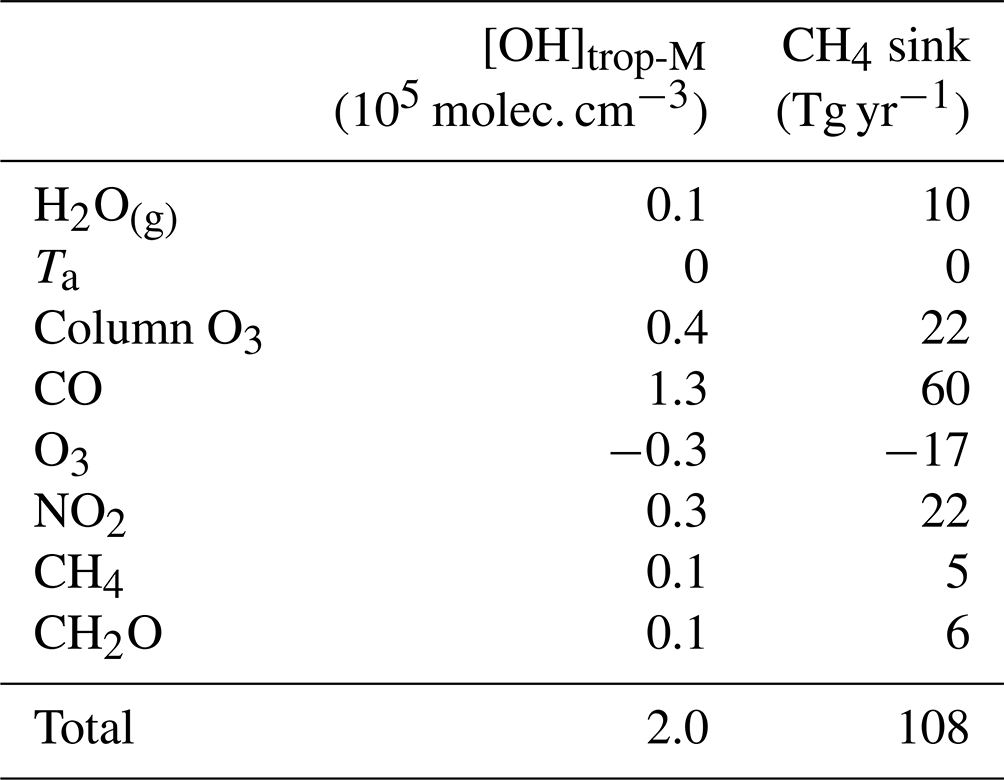
Reconciling the bottom-up and top-down estimates of the methane chemical sink is essential for a more accurate estimate of the global methane budget and to better attribute the observed changes in atmospheric growth rates of CH₄. One way to improve the bottom-up estimates of the CH₄ sink and thus reconcile the difference is to correct the OH simulated by atmospheric models using observations of OH precursors. Indeed, uncertainties in the OH simulated by atmospheric models can be attributed to biases in precursor concentrations. For example, Naik et al. (2013) found that an underestimation of carbon monoxide (CO) in the Northern Hemisphere can contribute to the overestimation of OH in this hemisphere; Strode et al. (2015) estimated that removing the model bias in O₃ and water vapor (H₂O_(g)) and reducing northern hemispheric nitrogen oxide (${\mathrm{NO}}_x=\mathrm{NO}+{\mathrm{NO}}_{\mathrm{2}}$) emissions can reduce a high bias in the global tropospheric OH burden by 10 %; Nicely et al. (2017, 2020) found that the inter-model difference in tropospheric OH is mainly driven by the difference in model-simulated ultraviolet light flux to the troposphere, the tropospheric O₃, CO, and NO_x mixing ratio. In addition, the budget analysis of OH production and loss showed that about 90 % of OH production is directly related to stratospheric and tropospheric ozone (O₃), H₂O_(g), and nitrogen oxide (NO), and ∼60 % of OH is removed by reaction with CO, CH₄, and formaldehyde (CH₂O) (Lelieveld et al., 2016; Zhao et al., 2020b). Thus, bottom-up estimates of the CH₄ sink from chemistry transport models (CTMs) can be improved if one can reduce the biases due to these OH precursors in modeled OH.

Fortunately, several satellites have collected long-term continuous observations of the aforementioned OH precursors with global coverage, providing the opportunity to evaluate and improve bottom-up estimates of the CH₄ sink. The chemistry reanalysis that assimilates satellite observations of O₃, CO, NO₂, nitric acid (HNO₃), and CO shows significant improvement on both global OH burden and inter-hemispheric gradient (Miyazaki et al., 2020). Such data-assimilation methods can well balance the model and observation uncertainties, but they are not easy to apply to different models that simulate the broad range of global OH burden (Naik et al., 2013; Zhao et al., 2019). In addition, they do not allow partitioning the OH bias due to each precursor. In this context, the main objective of this study is to explore a simple approach to reconcile bottom-up and top-down estimates of the CH₄ sink by (i) improving the simulated atmospheric OH fields using multiple satellite observations and meteorological data from reanalysis and (ii) assessing the contribution of each main OH precursor to the bias in simulated OH and CH₄ sink. As a result, top-down estimates of CH₄ emissions will also benefit from the improved 3D distributions of OH (Zhao et al., 2020a; Saunois et al., 2020). We first evaluate the OH precursors (CO, CH₄, O₃, CH₂O, and NO₂, the total column O₃, and H₂O_(g)) simulated for the year 2010 by the CESM1–CAM4Chem (Community Earth System Model using the Community Atmosphere Model version 4 as atmosphere component) and GEOSCCM (Goddard Earth Observing System Chemistry–Climate Model); these models participated in the CCMI-1 project, and they were used to estimate the global methane sink in Saunois et al. (2020) and represent two different chemical mechanisms. We then estimate the observation-based OH fields by correcting model biases of the two modeled OH fields due to the abovementioned OH precursors using the Dynamically Simple Model of Atmospheric Chemical Complexity (DSMACC). By doing so, we quantify the bias in tropospheric OH attributable to each precursor. Finally, we estimate the chemical sink of CH₄ using the observation-based OH field and, based on the uncertainties inferred for OH, we reveal the dominant factors contributing to the uncertainties in CH₄ chemical sink at the global and regional scales.

2 Method

2.1 Observational data

The total column O₃, which mainly influences the O (¹D) photolysis rate, is constrained by the National Aeronautics and Space Administration (NASA) Solar Backscatter Ultraviolet (SBUV) Merged Ozone Data Set (MOD) (Frith et al., 2014). The SBUV MOD column O₃ data are derived by combining observations from nine SBUV-type instruments aboard NASA's Aura satellite. The monthly O₃ columns are available for 5^∘ zonal mean.

Tropospheric O₃ is important in determining OH production. We constrain its spatial distributions using the tropospheric column O₃ data from the combined Aura Ozone Monitoring Instrument/Microwave Limb Sounder (OMI/MLS) satellite observations, which are generated by subtracting the co-located MLS limb measurements (integrated over the stratosphere to derive stratospheric column ozone) from total column ozone retrieved by OMI, a UV–Vis nadir solar backscatter spectrometer (Ziemke et al., 2006).

The tropospheric nitrogen oxide family (${\mathrm{NO}}_x=\mathrm{NO}+{\mathrm{NO}}_{\mathrm{2}}$) participates in both OH production – reaction of nitrogen oxide (NO) with hydroperoxyl radical (HO₂) or organic peroxy radicals (RO₂) – and loss (mainly reaction of NO₂ with OH). In the Dynamically Simple Model of Atmospheric Chemical Complexity (DSMACC) used in this study (see Sect. 2.3), the total reactive nitrogen (NO_y) is constrained by either NO₂ or NO concentrations. We constrain the spatial distributions of the boundary layer NO_y using satellite observations of NO₂ tropospheric vertical column density (VCD) of the QA4ECV (Quality Assurance for Essential Climate Variables) OMI NO₂ retrieval product (Boersma et al., 2018). Due to its short lifetime, NO_x emitted from the surface mainly remains within the planetary boundary layer (PBL). Thus, satellite-retrieved VCDs are widely used in understanding the NO₂ distributions within the boundary layer instead of the whole troposphere (e.g., Cooper et al., 2020; Geddes et al., 2017).

We also constrain tropospheric CO, CH₄, and CH₂O to better represent OH loss in the troposphere. Distributions of CO and CH₂O are taken from 4D variational data assimilation of the tropospheric CO column retrieved from the spaceborne MOPITT v7 instrument (Measurements Of Pollution In The Troposphere v7 TIR-NIR product; Deeter et al., 2017) and column CH₂O from the OMI version3 product (González Abad et al., 2015), respectively (Zheng et al., 2019). The CH₄ distributions are taken from data assimilation of surface CH₄ observations (Zhao et al., 2020a), mainly from the Earth System Research Laboratory of the US National Oceanic and Atmospheric Administration (NOAA/ESRL, Dlugokencky et al., 1994). The assimilated surface CO concentration and CH₄ profiles show good agreement with independent ground-based observations and aircraft observations, respectively (Zheng et al., 2019; Zhao et al., 2020a).

Meteorological conditions, mainly water vapor (H₂O_(g)) and air temperature (T_a) can also influence tropospheric OH. The H₂O_(g) (represented as specific humidity) and T_a are constrained by the second Modern-Era Retrospective analysis for Research and Applications (MERRA-2) reanalysis data from NASA's Global Modeling and Assimilation Office (GMAO) (Gelaro et al., 2017).

2.2 The 3D atmospheric chemistry model simulations

The 3D distributions of monthly mean OH fields and OH precursors for the year 2010 are taken from the REF-C1 experiment of the IGAC/SPARC Chemistry–Climate Model Initiative Phase-1 (CCMI-1; Hegglin and Lamarque, 2015; Morgenstern et al., 2017). The REF-C1 experiment is driven by state-of-the-art historical forcings and sea surface temperatures from observations and covers 51 years (1960–2010).

We include simulations from two models with different chemical mechanisms: (1) the Community Earth System Model (CESM) using the Community Atmosphere Model version 4 as atmosphere component (CESM1–CAM4Chem; Tilmes et al., 2015, 2016) and (2) the GEOS-5 Chemistry Climate Model (GEOSCCM; Molod et al., 2012, 2015; Oman et al., 2011, 2013; Nielsen et al., 2017). The tropospheric chemistry of CESM1–CAM4Chem is based on MOZART-4 mechanisms with minor updates (Emmons et al., 2010; Lamarque et al., 2012) and the GEOSCCM is based on the Global Modeling Initiative (GMI) chemistry and transport model (Duncan et al., 2007), which was originally developed for the GEOS-Chem model. The CO, NO₂, O₃, CH₄, CH₂O mixing ratios, total column O₃, and meteorological conditions including T_a and H₂O_(g) simulated by CESM1–CAM4Chem and GEOSCCM in 2010 are compared with the observational data described in Sect. 2.1 in the Supplement (Figs. S1–S3). We chose the CESM1–CAM4Chem and GEOSCCM in this study since (1) their global mean OH concentrations and OH distributions (both horizontal and vertical) are around the multi-model mean values given by Zhao et al. (2019), albeit not at the extreme of the model distribution; (2) the two models include multiple primary non-methane volatile organic compounds (NMVOC) emissions (Morgenstern et al., 2017); and (3) the chemical box model DSMACC already includes the MOZART-4 and GEOS-Chem chemical mechanisms (Sect. 2.3), which are similar to that used in CESM1 CAM4-Chem and GEOSCCM, respectively.

A detailed description of the two model settings related to OH and the CCMI-1 model experiments can be found in Morgenstern et al. (2017) and Zhao et al. (2019).

2.3 The chemical box model DSMACC

Differing from 3D atmospheric chemistry models, which simulate the OH by gridded emissions inventories of its precursors, a chemical box model simulates OH by prescribing precursor concentrations and the meteorological conditions. Thus, one can estimate the sensitivity of OH to different precursor concentrations and meteorological parameters. Here, we use the Dynamically Simple Model of Atmospheric Chemical Complexity (DSMACC; Emmerson and Evans, 2009) to estimate the sensitivity of OH to chemical species including CO, NO₂, O₃, CH₄, CH₂O, the total column O₃, and meteorological conditions including T_a and H₂O_(g), following the approach of Nicely et al. (2018).

The DSMACC model takes advantage of the kinetic preprocessor (KPP) to generate the FORTRAN code for a chosen chemical mechanism. In this study, the DSMACC model is compiled with MOZART-4 and GEOS-Chem chemical mechanisms, respectively, to be consistent with the associated 3D models CESM1–CAM4Chem and GEOSCCM. The clear-sky photolysis rates of chemical species are estimated by the tropospheric ultraviolet and visible (TUV) radiation model. Forced by meteorological variables (H₂O_(g), T_a, and pressure), total column O₃, and gas concentrations simulated by the CESM1–CAM4Chem and GEOSCCM or generated from observations, and the diurnal cycle of the photolysis rates estimated by the TUV radiation model, the DSMACC is run forward until reaching the diurnal steady state of OH. Nicely et al. (2018) have estimated the response of OH to changes in OH precursors by conducting DSMACC model simulations for broad latitude and pressure bins. The results show that the H₂O_(g), NO_x, total column O₃, and tropical expansion can lead to a positive trend in tropospheric OH, offsetting most of the negative trend led by the rising CH₄ concentrations from 1980 to 2015. Here, for each month, we run the DSMACC model for each model pixel of the 3D grid to better represent the heterogeneous spatial distributions of OH. For example, the CESM1–CAM4Chem has 144 (longitude) × 96 (latitudes) × 13 (pressure level) model grids in the troposphere. For each sensitivity experiment (Sect. 2.4), we therefore conduct 179 712 DSMACC model simulations (for the CESM1–CAM4Chem grid) each month.

Table 1 The DSMACC model experiments.

2.4 DSMACC experiments

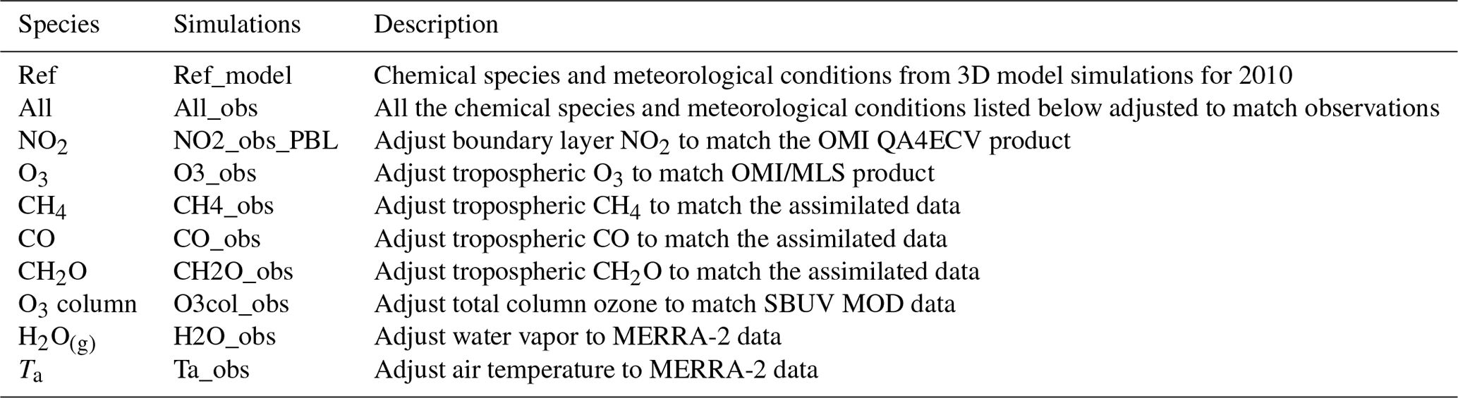
Table 1 lists the experiments conducted with the DSMACC chemical box model. The reference experiment (Ref_model in Table 1) is conducted by running the DSMACC model with the monthly mean chemical species concentrations and meteorological conditions simulated by the 3D models (CESM1–CAM4chem/GEOSCCM) for each pixel in 2010 using the corresponding chemical mechanisms. During the DSMACC simulation for each month, the meteorological conditions and chemical species with a lifetime of a few hours (e.g., NMVOCs) to several years (e.g., CH₄) are set to the monthly mean values from 3D model outputs and unchanged during the simulation. We estimated the diurnal steady-state solution for the chemical species with a short lifetime of a few seconds (e.g., OH and HO₂ radicals). Since most of the CCMI models provide the 3D distributions of the chemical species on monthly time resolution, the influence of sub-monthly variations such as the diurnal cycle for these chemical species and meteorological conditions on OH concentrations are not represented in the DSMACC simulations. In the All_obs simulation, the CO, NO₂, O₃, CH₄, and CH₂O, total column O₃, T_a, and H₂O_(g) are replaced with the available observation-based data for 2010, while other DSMACC inputs (pressure and other chemical species) are the same as in the Ref_model simulation. For CO, CH₄, CH₂O, and meteorological conditions, the observation-based data are taken directly from the monthly mean of the assimilated or reanalysis data as described in Sect. 2.2 (regrid to model horizontal and vertical grid). For tropospheric NO₂ and O₃, we use satellite data to generate the observation-based DSMACC input. The associated uncertainties of using the satellite observations of O₃ and NO₂ at overpass time are discussed in Sect. 4.3. As the satellite observations provide the tropospheric VCDs, the observation-based concentrations are estimated by combining the satellite-observed tropospheric columns and model-simulated vertical distributions. We estimate the tropospheric column density simulated by atmospheric chemistry models (C_{trop_model}) using the tropopause pressure estimated based on the WMO (World Meteorological Organization, 1957) tropopause definition. Then, we estimate the scaling factor for each model horizontal grid cell as the ratio of satellite observations (C_{trop_obs}) to the modeled tropospheric column density (C_{trop_model}). The observation-based concentration (C_{grid_obs}) in each model pixel, which is used as the DSMACC input, is then estimated by multiplying the corresponding model-simulated concentration (C_{grid_model}) by the scaling factor:

$$\begin{array}{}\text{(1)}& C_{\mathrm{grid}\mathrm{\_}\mathrm{obs}}=C_{\mathrm{grid}\mathrm{\_}\mathrm{model}}\times {\displaystyle \frac{C_{\mathrm{trop}\mathrm{\_}\mathrm{obs}}}{C_{\mathrm{trop}\mathrm{\_}\mathrm{model}}}}.\end{array}$$

For O₃, we estimate the C_{grid_obs} for each 3D model pixel in the whole troposphere using Eq. (1). For NO₂, we only estimate C_{grid_obs} in the boundary layer (the boundary layer height is from the MERRA-2 reanalysis data) since the NO₂ emitted from the surface mainly remains within the boundary layer.

Table 2 Modeled and observation-based estimates of global [OH]_trop-M, CH₄ sink by tropospheric OH ($L_{{\mathrm{CH}}_{\mathrm{4}}+\mathrm{OH}}$) averaged during 2000–2009, and the CH₄ lifetime against tropospheric OH (${\mathit{\tau }}_{{\mathrm{CH}}_{\mathrm{4}}+\mathrm{OH}}$).

The Ref_model experiments can well reproduce the spatial distribution of [OH]_trop-M simulated by 3D models (Fig. S4), which indicate that the chemical box model DSMACC can generally capture the response of OH to the changes in OH precursor concentrations and meteorological conditions. However, the Ref_model experiments overestimate the [OH]_trop-M by 7 % and 36 % when compared with the global [OH]_trop-M simulated by CESM1–CAM4Chem and GEOSCCM, respectively. Thus, the observation-based OH ([OH]_obs) in each 3D model pixel for two different chemical mechanisms is estimated by correcting OH as simulated by the corresponding 3D models ([OH]_model) by the ratio between OH simulated by DSMACC experiments for the All_obs ([OH]_{DSMACC_all_obs}) and for the Ref_model ([OH]_{DSMACC_Ref_model}) case:

$$\begin{array}{}\text{(2)}& [\mathrm{OH}{]}_{\mathrm{obs}}=[\mathrm{OH}{]}_{\mathrm{model}}\times {\displaystyle \frac{[\mathrm{OH}{]}_{\mathrm{DSMACC}\mathrm{\_}\mathrm{all}\mathrm{\_}\mathrm{obs}}}{[\mathrm{OH}{]}_{\mathrm{DSMACC}\mathrm{\_}\mathrm{Ref}\mathrm{\_}\mathrm{model}}}}.\end{array}$$

Then, we also perform eight sensitivity experiments (xk_obs in Table 1) that only adjust one individual chemical species or meteorological condition (here and after represented as x_k) to the observations (obs), keeping the other parameters equal to the simulated values from the chemistry–climate model. Because of high computing costs, we conduct the sensitivity experiments using only CESM1–CAM4C-chem outputs. The OH biases due to each factor (δ[OH]_xk) are estimated by introducing the OH simulated in the sensitivity experiment xk_obs ([OH]_{DSMACC_xk_obs}) as:

$$\begin{array}{}\text{(3)}& {\displaystyle }& {\displaystyle }[\mathrm{OH}{]}_{\mathrm{xk}\mathrm{\_}\mathrm{obs}}=[\mathrm{OH}{]}_{\mathrm{model}}\times {\displaystyle \frac{[\mathrm{OH}{]}_{\mathrm{DSMACC}\mathrm{\_}\mathrm{xk}\mathrm{\_}\mathrm{obs}}}{[\mathrm{OH}{]}_{\mathrm{DSMACC}\mathrm{\_}\mathrm{Ref}\mathrm{\_}\mathrm{model}}}},\text{(4)}& {\displaystyle }& {\displaystyle }\mathit{\delta }[\mathrm{OH}{]}_{x_k}=[\mathrm{OH}{]}_{\mathrm{model}}-[\mathrm{OH}{]}_{\mathrm{xk}\mathrm{\_}\mathrm{obs}}.\end{array}$$

2.5 Chemical loss of CH₄

We estimate the yearly tropospheric chemical loss of CH₄ through reaction with OH ($L_{{\mathrm{CH}}_{\mathrm{4}}+\mathrm{OH}}$) at global and regional scale from 2000 to 2009 by integrating the reaction of CH₄ with OH:

$$\begin{array}{}\text{(5)}& L_{{\mathrm{CH}}_{\mathrm{4}}+\mathrm{OH}}=\sum _i\sum _{t}K\left(T_{\mathrm{a}}\right)m\left({\mathrm{CH}}_{\mathrm{4}}\right)\left[\mathrm{OH}\right]\mathit{\delta }t,\end{array}$$

where i is the index of the model pixel in the troposphere and δt is the integration time step (3 h). The monthly 3D distributions of CH₄ mass (m(CH₄)) during 2000–2009 are from data assimilation of surface CH₄ observations from NOAA/ESRL (Dlugokencky et al., 1994) and the T_a distributions are from MERRA-2 reanalysis data (see Sect. 2.2). The reaction rate K(T_a) is a function of T_a as given by Sander et al. (2011):

$$\begin{array}{}\text{(6)}& K\left(T_{\mathrm{a}}\right)=\mathrm{2.45}\times {\mathrm{10}}^{-\mathrm{12}}{e}^{-\frac{\mathrm{1775}}{T_{\mathrm{a}}}}.\end{array}$$

The contribution of each factor x_k to the bias in chemical loss of CH₄ through reaction with OH ($\mathit{\delta }{L}_{{\mathrm{CH}}_{\mathrm{4}}+\mathrm{OH}\mathrm{\_}\mathrm{xk}}$) can be estimated as:

$$\begin{array}{}\text{(7)}& \mathit{\delta }{L}_{{\mathrm{CH}}_{\mathrm{4}}+\mathrm{OH}\mathrm{\_}\mathrm{xk}}=\sum _i\sum _{t}K\left(T_{\mathrm{a}}\right)m\left({\mathrm{CH}}_{\mathrm{4}}\right)\mathit{\delta }[\mathrm{OH}{]}_{x_k}\mathit{\delta }t,\end{array}$$

with $L_{{\mathrm{CH}}_{\mathrm{4}}+\mathrm{OH}}$, we further estimate the CH₄ lifetime to reaction with tropospheric OH (${\mathit{\tau }}_{{\mathrm{CH}}_{\mathrm{4}}+\mathrm{OH}}$) through the global CH₄ burden:

$$\begin{array}{}\text{(8)}& {\mathit{\tau }}_{{\mathrm{CH}}_{\mathrm{4}}+\mathrm{OH}}={\displaystyle \frac{\sum _{j}m\left({\mathrm{CH}}_{\mathrm{4}}\right)}{L_{{\mathrm{CH}}_{\mathrm{4}}+\mathrm{OH}}}},\end{array}$$

where j is the index of the model pixel in the entire atmosphere.

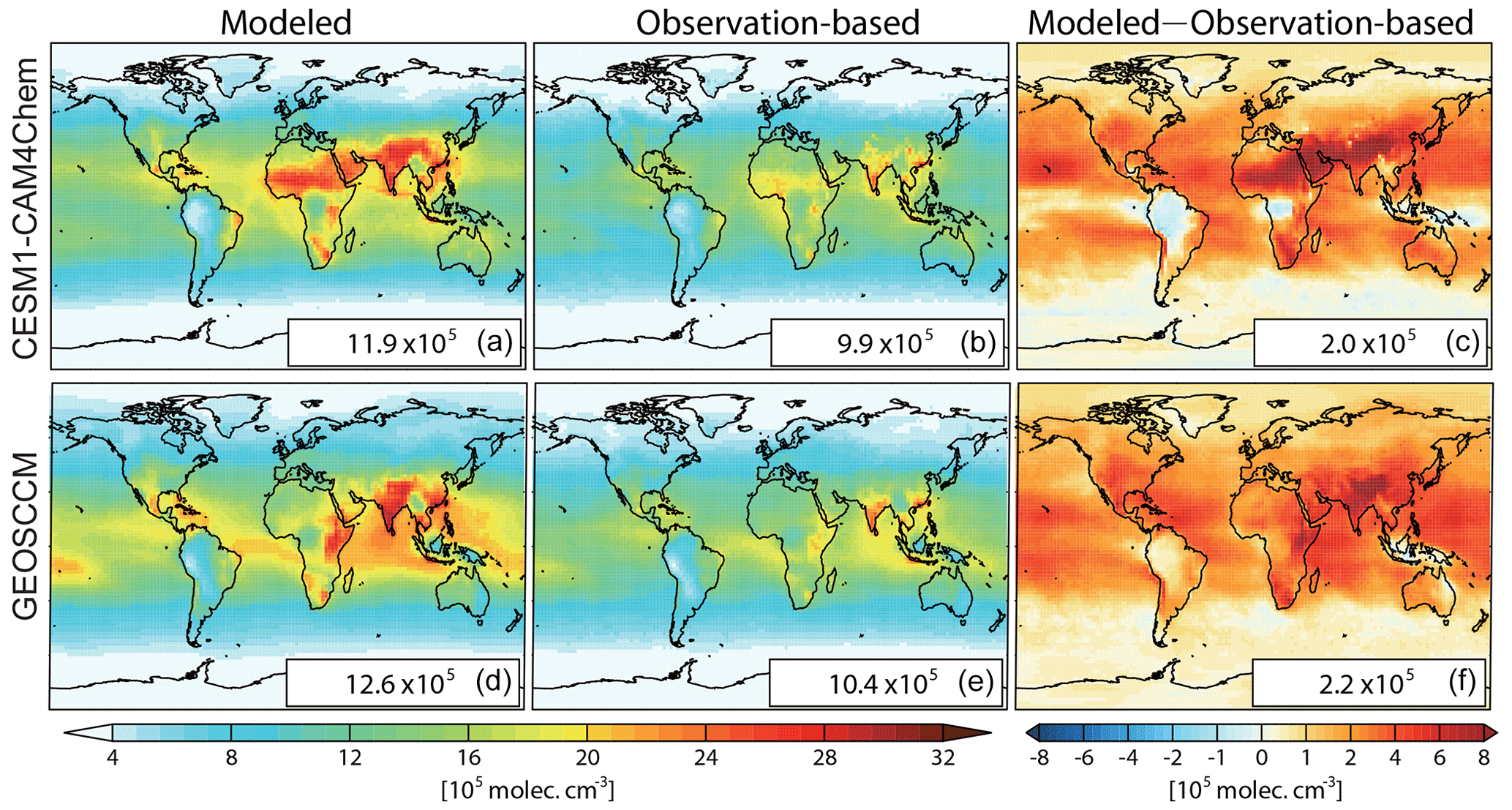
Figure 1 Spatial distributions of air-mass-weighted tropospheric mean OH ([OH]_trop-M) in 2010 from model simulations (a, d) and constrained by observations (b, e), and the difference between modeled and observation-based [OH]_trop-M (c, f) estimated from CESM1–CAM4Chem (a–c) and GEOSCCM (d–f) simulations. The global mean values are shown in the inset in molec. cm⁻³.

3 Results

3.1 Observation-based tropospheric OH

3.1.1 Global tropospheric OH burden

The global mean tropospheric column-averaged air-mass-weighted OH ([OH]_trop-M) simulated by CESM1–CAM4Chem and GEOSCCM in 2010 are 11.9×10⁵ and 12.6×10⁵ molec. cm⁻³, respectively. By adjusting OH precursors and meteorological conditions (total column O₃, tropospheric O₃, CO, CH₄, CH₂O, boundary layer NO₂, H₂O_(g), and T_a) to the observations using the DSMACC model, we estimated the observation-based [OH]_trop-M to be9.9×10⁵ and 10.4×10⁵ molec. cm⁻³ with CESM1–CAM4Chem and GEOSCCM chemical mechanisms, respectively (Fig. 1 and Table 2). Compared with the original OH fields simulated by CESM1–CAM4Chem and GEOSCCM, the observation-based OH fields reduce the model-simulated global [OH]_trop-M by $\sim \mathrm{2}\times {\mathrm{10}}^{\mathrm{5}}$ molec. cm⁻³. The global [OH]_trop-M estimated by the observation-based OH fields in this study is lower than the value estimated by Spivakovsky et al. (2000) (11.6×10⁵ molec. cm⁻³), which is used in the chemistry transport model (CTM) intercomparison experiment (TransCom-CH4) after being scaled by a factor of 0.92 (Patra et al., 2011) but consistent with those estimated by MCF-based inversions ($\sim \mathrm{10}\times {\mathrm{10}}^{\mathrm{5}}$ molec. cm⁻³; Bousquet et al., 2005; Krol and Lelieveld, 2003). The consistency with the MCF-based estimates indicates that our approach (correcting model bias through available observations) is capable of capturing the global OH burden.

3.1.2 The OH spatial distribution

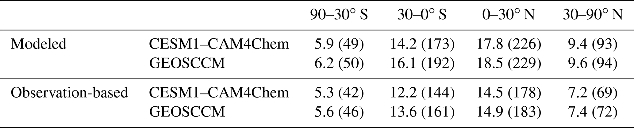
Figures 1 and 2 show the spatial distribution and zonal average of the [OH]_trop-M, respectively, estimated from the observation-based and original model-simulated OH fields. The observation-based OH fields show similar spatial distributions as their respective original model simulations, with high [OH]_trop-M (10–15×10⁵ molec. cm⁻³) over East Asia, South Asia, and northern Africa, corresponding to the regions with high tropospheric O₃, NO₂, and H₂O_(g) (Figs. S1 and S3). The lowest [OH]_trop-M is found over the high latitudes ($<\mathrm{4}\times {\mathrm{10}}^{\mathrm{5}}$ molec. cm⁻³) due to less ultraviolet radiation and over the Amazon forest (4–8×10⁵ molec. cm⁻³) due to high biogenic non-methane volatile organic compound (NMVOC) emissions. The observation-based [OH]_trop-M averaged over the northern tropics (0–30^∘ N) and northern middle to high latitudes (30–90^∘ N) are $>\mathrm{14}\times {\mathrm{10}}^{\mathrm{5}}$ and $>\mathrm{7}\times {\mathrm{10}}^{\mathrm{5}}$ molec. cm⁻³, respectively, for both chemical mechanisms, which are higher than those over the southern tropics (12.2–13.6×10⁵ molec. cm⁻³) and southern middle to high latitudes (5.3–5.6×10⁵ molec. cm⁻³, Table 3 and Fig. 2). The two observation-based OH fields show similar mean [OH]_trop-M over most of the latitudinal bands, except for the southern tropics (0–30^∘ S), where the mean [OH]_trop-M estimated by the GEOSCCM chemical mechanism is 1.4×10⁵ molec. cm⁻³ higher than the one from CESM1–CAM4Chem (Table 3 and Fig. 2).

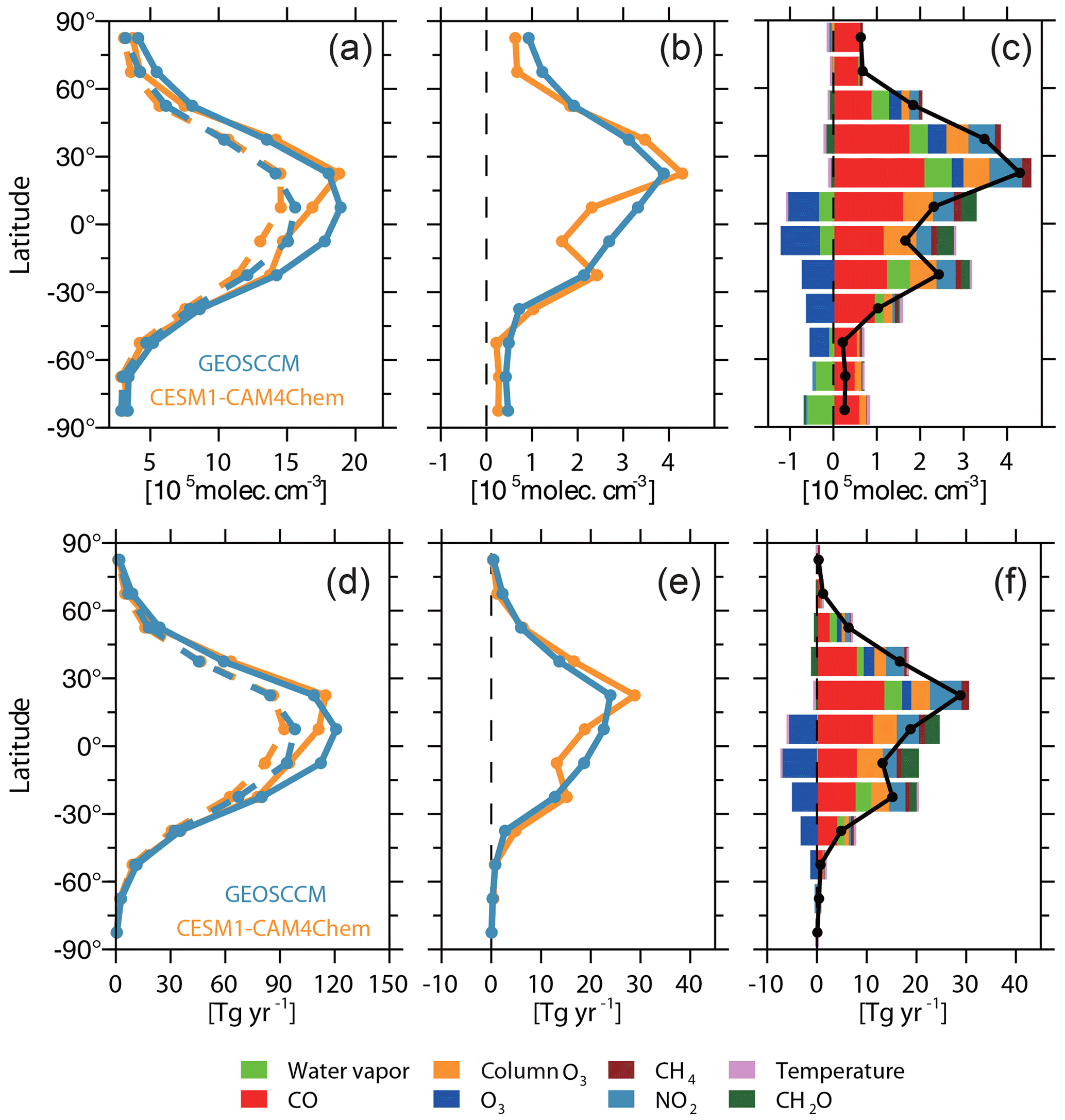
Figure 2 (a) Zonal-averaged [OH]_trop-M of modeled (solid lines) and observation-based OH field (dashed lines) estimated from CESM1–CAM4Chem (yellow) and GEOSCCM (blue) simulations. (b) Difference of zonal-averaged [OH]_trop-M between modeled and observation-based OH fields. (c) Difference between CESM1–CAM4Chem simulated and observation-based zonal-averaged [OH]_trop-M (black line) and the contribution from each OH precursor (colored bars) to zonal-averaged difference. (d–f) Same as (a–c) but for the tropospheric CH₄ sink by reaction with OH.

Table 3 The modeled and observation-based [OH]_trop-M (in 10⁵ molec. cm⁻³) averaged over latitudinal bands during 2000–2009. The corresponding tropospheric CH₄ sink by OH ($L_{{\mathrm{CH}}_{\mathrm{4}}+\mathrm{OH}}$) (in Tg yr⁻¹) is given in brackets.

Compared to the original [OH]_trop-M simulated by CESM1–CAM4Chem and GEOSCCM, adjusting to observations reduces the [OH]_trop-M by 2–8×10⁵ molec. cm⁻³ over most regions except the tropical forests. The reduction of mean [OH]_trop-M over the northern tropics (0–30^∘ N) and middle to high latitudes (30–90^∘ N) are $>\mathrm{3}\times {\mathrm{10}}^{\mathrm{5}}$ and $>\mathrm{2}\times {\mathrm{10}}^{\mathrm{5}}$ molec. cm⁻³, respectively, which is larger than that over the southern tropics (0–30^∘ S by $\sim \mathrm{2}\times {\mathrm{10}}^{\mathrm{5}}$ molec. m⁻³) and middle to high latitudes (30–90^∘ S by 0.6×10⁵ molec. cm⁻³). The Northern Hemisphere to Southern Hemisphere ($\mathrm{N}/\mathrm{S}$) ratios of the simulated OH fields are reduced from 1.35 to 1.24 for CESM1–CAM4Chem and 1.26 to 1.15 for GEOSCCM. Although the $\mathrm{N}/\mathrm{S}$ ratios of the observation-based OH fields are still higher than the 1, which is obtained from MCF-based inversions (Bousquet et al., 2005; Patra et al., 2014), incorporating available observations has significantly reduced the model-simulated $\mathrm{N}/\mathrm{S}$ ratio.

The spatial distribution of the observation-based OH of this study is different from the OH field estimated by Spivakovsky et al. (2000). The OH field estimated by Spivakovsky et al. (2000) shows a high [OH]_trop-M over the regions with biomass burning emissions (Fig. S5). Instead of considering the detailed spatial distributions of nitrogen oxides, Spivakovsky et al. (2000) use a series of NO_y profiles for land and ocean over large regions (Fig. S6). As shown in Figs. S5 and S6, the highest [OH]_trop-M over South America and Africa estimated by Spivakovsky et al. (2000) correspond to high NO_y mixing ratios over these two regions. The OH shows high positive sensitivity to NO_y in the free troposphere due to low VOCs and NO_y mixing ratios (Fig. S7). Using satellite observations, Choi et al. (2014) showed that the high NO₂ mixing ratios in the free troposphere are mainly located near polluted urban regions (e.g., North America, Europe, and Asia), which is more similar to the NO₂ distribution simulated by 3D atmospheric models (Fig. S1). Thus, although the OH field estimated by Spivakovsky et al. (2000) gives an $\mathrm{N}/\mathrm{S}$ ratio of 1, its spatial distribution may have biases due to the simplification in the NO_y distributions.

3.2 Contribution from individual factors to model biases in [OH]_trop-M

By conducting the sensitivity simulations listed in Table 1, we estimate the contribution of individual factors to model biases based on Eqs. (3) and (4). The sensitivity of OH to model biases in tropospheric O₃, stratospheric O₃, H₂O_(g), and NO_x emissions have been tested in Strode et al. (2015) using GEOSCCM. In this section, we extend the procedure of Strode et al. (2015) by including more factors: T_a, CO, CH₂O, CH₄, and NO₂ in the boundary layer.

Table 4 summarizes the contribution of each chemical precursor and meteorological condition to the difference between CESM1–CAM4Chem simulated and observation-based global [OH]_trop-M. On the global scale, the total contribution of the eight individual factors to the difference in [OH]_trop-M estimated from the simulation xk_obs is 2.0×10⁵ molec. cm⁻³ (Table 4), consistent with that estimated from the simulation All_obs (Table 2). On the regional scale, they show small differences (usually <10 % of the signal, Fig. S8), which can be attributed to the nonlinear chemistry. Indeed, although the atmospheric OH is produced and removed through complex nonlinear chemical reactions, one can infer the large-scale [OH]_trop-M changes by roughly summing the influence from individual factors.

Table 4 Contributions from individual factors to the difference in global [OH]_trop-M and tropospheric CH₄ sink by reaction with OH between CESM1–CAM4Chem simulated and the corresponding observation-based OH fields (modeled–observation-based).

3.2.1 Contribution from CO

CO is the largest OH sink in the troposphere (Lelieveld et al., 2016; Zhao et al., 2020b). The sensitivity simulation CO_obs shows that a 1 ppbv increase in CO can result in a decrease in OH by up to more than 3×10⁴ molec. cm⁻³ (Fig. S7). Compared with the CO distributions from inversions that assimilated MOPITT observations, the CESM1–CAM4Chem underestimates the global tropospheric mean CO mixing ratio by 24 ppbv (Fig. S1). Based on the DSMACC simulations CO_obs and Ref_CESM (Table 1), we find that the negative bias in CO contributes most to the difference in the modeled versus observation-based [OH]_trop-M (1.3×10⁵ molec. cm⁻³; Table 4 and Fig. 3). The underestimation of CO is common in atmospheric models and was treated either as a cause or an effect of the overestimated OH in previous studies (Naik et al., 2013; Monks et al., 2015; Strode et al., 2015). For example, based on the Atmospheric Chemistry and Climate Model Intercomparison Project (ACCMIP) simulations, Naik et al. (2013) found that the positive bias in OH was most likely due to the underestimation of CO when compared with both satellite and surface observations. In contrast, Strode et al. (2015) did sensitivity simulations using the GEOSCCM model and showed that reducing OH bias could improve the accuracy of modeled CO. In this study, we do not intend to solve the cause-and-effect issue between CO and OH since the discrepancy in [OH]_trop-M of 1.3×10⁵ molec. cm⁻³ could also be understood as the global tropospheric [OH] changes that would be needed to simulate the observed CO.

Figure 3 Spatial distributions of the contribution of individual factors to the difference between CESM1–CAM4Chem simulated and observation-based (modeled–observation-based) [OH]_trop-M. The global mean values are shown inset in molec. cm⁻³.

The underestimation of the CO mixing ratio is larger over the Northern Hemisphere (30 ppbv) than over the Southern Hemisphere (18 ppbv) (Fig. S1). The largest bias in [OH]_trop-M induced by CO is found over the northern tropics (1.9×10⁵ molec. cm⁻³) followed by those over the northern middle to high latitude regions and the southern tropics (1.2×10⁵ molec. cm⁻³; Fig. 2). Naik et al. (2013) demonstrated that the model bias in CO contributes to the overestimation of the modeled $\mathrm{N}/\mathrm{S}$ ratio in [OH]_trop-M. In this study, although the underestimation of CO leads to a larger positive bias of [OH]_trop-M over the Northern Hemisphere than the Southern Hemisphere, the observation-based adjustment only reduces the positive bias of the $\mathrm{N}/\mathrm{S}$ ratio by 0.02. This means that the $\mathrm{N}/\mathrm{S}$ difference of the CO bias is not sufficient to explain the inconsistency between the CESM1–CAM4Chem simulated and MCF-based $\mathrm{N}/\mathrm{S}$ ratio in [OH]_trop-M.

3.2.2 Contribution from tropospheric O₃

Tropospheric O₃ can contribute to both primary and secondary OH production. Compared to satellite observations from OMI, CESM1–CAM4Chem simulations show a large overestimation of tropospheric O₃ over the 15–60^∘ N region (up to 14 DU, 40 %) and an underestimation (14 DU, 40 %) over the tropics and Southern Hemisphere (Fig. S1).

At the global scale, the model bias in O₃ leads to a negative bias on [OH]_trop-M by 0.3×10⁵ molec. cm⁻³, much smaller than that caused by CO (Table 4). However, at the regional scale, The CESM1–CAM4Chem simulated [OH]_trop-M is enhanced by $\sim \mathrm{1}\times {\mathrm{10}}^{\mathrm{5}}$ molec. cm⁻³ over the tropics (15^∘ S–15^∘ N) and $\sim \mathrm{0.5}\times {\mathrm{10}}^{\mathrm{5}}$ molec. cm⁻³ over the mid-Southern Hemisphere (15–60^∘ S), while it is reduced by 0.1–0.3×10⁵ molec. cm⁻³ over the mid-Northern Hemisphere (15–60^∘ N) when adjusted to OMI/MLS tropospheric column O₃ (Fig. 2). The adjustment reduces the $\mathrm{N}/\mathrm{S}$ ratio of [OH]_trop-M by 0.07; however, it still cannot explain the overestimation of the $\mathrm{N}/\mathrm{S}$ ratio but leads to a larger correction than the one with CO alone.

3.2.3 Contribution from boundary layer NO₂

The sensitivity of OH to NO₂ is highly variable. We estimate that a 1 ppbv increase in NO₂ can lead to a change of OH ranging from $-\mathrm{3}\times {\mathrm{10}}^{\mathrm{6}}$ molec. cm⁻³ to more than $+\mathrm{10}\times {\mathrm{10}}^{\mathrm{6}}$ molec. cm⁻³, depending on the mixing ratio of NMVOCs (represented as HCHO+isoprene) and NO₂ (Fig. S7). Compared to the QA4ECV NO₂ retrieval product, CESM1–CAM4Chem overestimates tropospheric NO₂ over most regions except northern China and tropical forests (Fig. S1).

At the global scale, the overestimation of NO₂ leads to a positive bias in [OH]_trop-M by 0.3×10⁵ molec. cm⁻³ (Table 4). At the regional scale, correcting for the PBL NO₂ does not influence the $\mathrm{N}/\mathrm{S}$ ratio of OH. As shown in Fig. 3, the overestimation of PBL NO₂ results in a positive bias in [OH]_trop-M over most of the continental regions. Over tropical and temperate oceans, one can also see that the slight overestimation in NO₂ leads to a significate positive bias in OH by 0.5–1×10⁵ molec. cm⁻³ since the sensitivity of [OH]_trop-M to NO₂ can be very high (10⁷ molec. cm⁻³ ppbv⁻¹ NO₂) over the regions with low NO_x and NMVOC mixing ratios. Over northern China, although the model shows a large underestimation in NO₂ (Fig. S1), the [OH]_trop-M is slightly smaller after adjustment. This is because the OH is not sensitive to an increase in NO₂ over high NO₂ regions or even shows a negative response (Fig. S7).

3.2.4 Contribution from total column O₃

Total column O₃ mainly influences O¹(D) photolysis through absorbing UV radiation. The CESM1–CAM4Chem simulation mainly underestimates the total O₃ columns by up to ∼10 DU over tropical regions compared with the SBUV MOD observations (Fig. S2). On a global scale, the underestimation of the total column O₃ can lead to an overestimation of the [OH]_trop-M by 0.4×10⁵ molec. cm⁻³ (Table 4 and Fig. 3), comparable with that due to tropospheric O₃.

3.2.5 Contribution from CH₄ and CH₂O

In CCMI-1 simulations, atmospheric chemistry models prescribe the lower boundary conditions for CH₄ following the Representative Concentration Pathway (RCP6.0). Compared to the posterior CH₄ fields from inversions by assimilating the surface CH₄ observations, the tropospheric mean CH₄ mixing ratios used in the CESM–CAM4Chem are ∼80 ppbv lower over the tropical and extratropical regions with high biomass burning and anthropogenic emissions and ∼40 ppbv lower over other regions. However, due to the low sensitivity of [OH] to CH₄ changes (Fig. S1), the underestimation in CH₄ only leads to a small positive bias in the global mean [OH]_trop-M by 0.1×10⁵ molec. cm⁻³.

The CESM1–CAM4Chem overestimates CH₂O by more than 50 % over land but slightly underestimates CH₂O over tropical oceans (Fig. S1). Since CH₂O contributes to only a small part (6 %) of the total OH loss (Zhao et al., 2020b), the large bias in the CESM1–CAM4Chem simulated CH₂O only leads to a small positive bias global mean [OH]_trop-M by 0.1×10⁵ molec. cm⁻³ (Fig. 3).

3.2.6 Contribution from meteorological conditions

H₂O_(g) is a major OH precursor that contributes to the primary production of OH and T_a can influence OH production and loss rates. Compared to MERRA-2 reanalysis data, CESM1–CAM4Chem overestimates zonally averaged H₂O_(g) mixing ratios near the surface and around 800 hPa by ∼1.5 g kg⁻¹ (Fig. S3). The sensitivity experiments show that a change in specific humidity by 1 g kg⁻¹ can lead to a change in OH by $>\mathrm{3}\times {\mathrm{10}}^{\mathrm{5}}$ molec. cm⁻³ over the regions with high O(¹D) photolysis and low NMVOC mixing ratios (Fig. S7). As shown in Table 4 and Fig. 3, globally, the model bias in H₂O_(g) only leads to a small bias (0.1×10⁵ molec. cm⁻³) [OH]_trop-M, but regionally, the model bias in H₂O_(g) can lead to a bias in [OH]_trop-M by the magnitude of 5×10⁵ molec. cm⁻³, even larger than that induced by the bias in CO. For T_a, the model only shows a small bias (<1 ^∘C) compared with MERRA-2 reanalysis data (Fig. S3). Thus, model bias in [OH]_trop-M induced by T_a is negligible (Fig. 3).

3.3 Chemical sinks of CH₄ as estimated by observation-based OH fields

3.3.1 Global and regional OH chemical sink of CH₄

Using the observation-based OH field, we estimate that the global tropospheric CH₄ loss by reaction with tropospheric OH ($L_{{\mathrm{CH}}_{\mathrm{4}}+\mathrm{OH}}$) averaged during the period 2000 through 2009 is 434 and 461 Tg yr⁻¹ for CESM1–CAM4Chem and GEOSCCM, respectively. These estimates are about 105 Tg yr⁻¹ lower than estimated by the original model-simulated OH fields (540 and 565 Tg yr⁻¹, respectively; Table 2). The corresponding CH₄ lifetimes against tropospheric OH loss estimated by the two observation-based OH fields are 11.4 and 10.7 year for CESM1–CAM4Chem and GEOSCCM, respectively, well within the range estimated by Prather et al. (2012) based on the MCF-inversions (11.2±1.3 yr) and much longer than estimated by the original model-simulated OH fields (9.1 years for CESM1–CAM4Chem and 8.7 years for GEOSCCM).

As shown in Table 3, more than 70 % of the tropospheric $L_{{\mathrm{CH}}_{\mathrm{4}}+\mathrm{OH}}$ occurs over tropical regions mainly due to both high OH and T_a. Constraining the tropospheric OH by precursor concentrations reduces the tropospheric $L_{{\mathrm{CH}}_{\mathrm{4}}+\mathrm{OH}}$ by ∼30 Tg yr⁻¹ (16 %) over the southern tropics, ∼50 Tg yr⁻¹ (21 %) over the northern tropics, and ∼25 Tg yr⁻¹ (25 %) over the northern middle to high latitude as estimated by both CESM1–CAM4Chem and GEOSCCM OH fields. Over the southern middle- to high-latitude regions, there are only limited changes (∼5 Tg yr⁻¹) in tropospheric $L_{{\mathrm{CH}}_{\mathrm{4}}+\mathrm{OH}}$. Thus, constraining tropospheric OH by precursor concentrations changes the inter-hemispheric distribution of $L_{{\mathrm{CH}}_{\mathrm{4}}+\mathrm{OH}}$. The values of $L_{{\mathrm{CH}}_{\mathrm{4}}+\mathrm{OH}}$ estimated by the observation-based OH fields are ∼35 and ∼75 Tg yr⁻¹ lower than that estimated by the corresponding original model-simulated OH fields over the Southern and Northern Hemisphere, respectively (Table 3). Thus, the inter-hemispheric difference of $L_{{\mathrm{CH}}_{\mathrm{4}}+\mathrm{OH}}$ (north–south) estimated by observation-based OH fields (60 Tg yr⁻¹ by CESM1–CAM4Chem and 48 Tg yr⁻¹ by GEOSCCM) is ∼40 % lower than estimated by the original model-simulated OH fields (98 Tg yr⁻¹ by CESM1–CAM4Chem and 81 Tg yr⁻¹ by GEOSCCM).

3.3.2 Global total chemical sink of CH₄

We estimate the global total CH₄ chemical sink for 2000–2009 by gathering (1) the tropospheric $L_{{\mathrm{CH}}_{\mathrm{4}}+\mathrm{OH}}$ estimated using the original model-simulated and observation-based OH fields, (2) the CH₄ loss in the stratosphere (26 Tg yr⁻¹ estimated by CESM1 CAM4-chem and 36 Tg yr⁻¹ estimated by GEOSCCM simulations) and CH₄ oxidized by chlorine (11 Tg yr⁻¹) given by Saunois et al. (2020). We then compare the chemical sink estimated in this study with that estimated by the bottom-up and top-down methods given by the previous GCP global CH₄ budget (Saunois et al., 2016, 2020).

As shown in Fig. 4, the bottom-up estimates in the GCP global CH₄ budget (blue bars) have a large range (483–738 Tg yr⁻¹ in Saunois et al., 2016 and 489–749 Tg yr⁻¹ in Saunois et al., 2020), much higher than those from the top-down method (514 Tg yr⁻¹ in Saunois et al., 2016 and 459–516 Tg yr⁻¹ in Saunois et al., 2020). The CH₄ sinks simulated by CESM1–CAM4Chem (549 Tg yr⁻¹) and GEOSCCM (585 Tg yr⁻¹) were included in the bottom-up estimates in Saunois et al. (2020) (green bar) and are slightly lower than the average value estimated using different OH fields (595 Tg yr⁻¹).

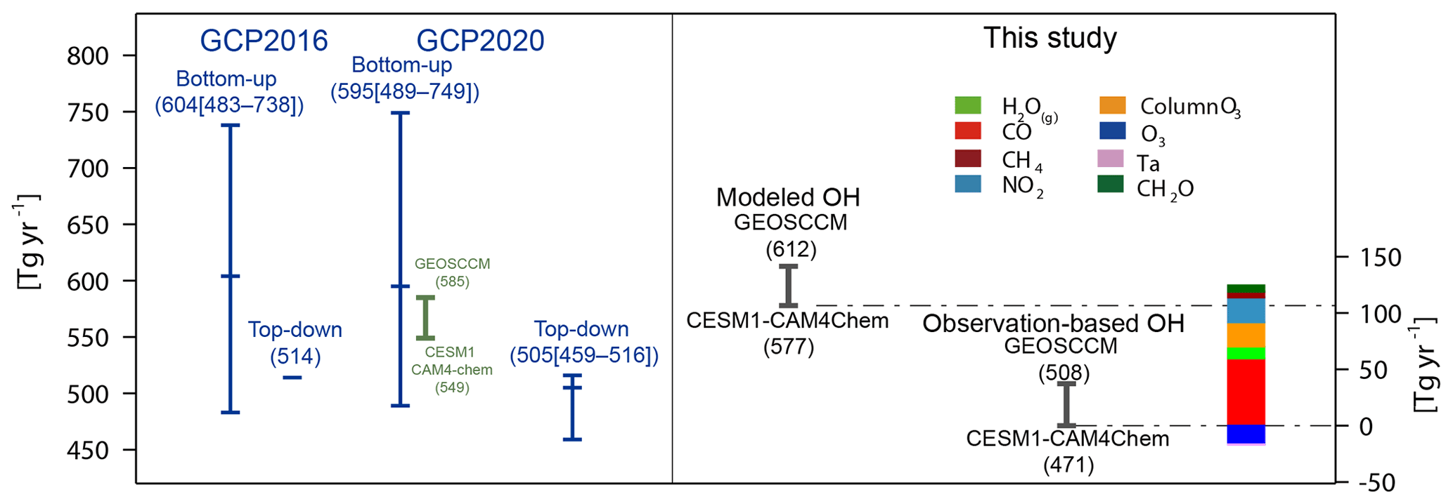
Figure 4 Global total chemical loss of CH₄ estimated by the bottom-up and top-down methods from the previous GCP global CH₄ budget (blue bars; Saunois et al., 2016, 2020), simulated by GEOSCCM and CESM1–CAM4Chem which is included in the bottom-up estimates in Saunois et al. (2020) (green bar), and that estimated in this study using the model-simulated and observation-based OH fields and CH₄ distributions assimilated surface observations (black bars). The colored bar shows the contribution of individual factors to the difference in the chemical loss of CH₄ between CESM1–CAM4Chem simulated and the corresponding observation-based OH. The blue, green, and black bars correspond to the left axis, and the colored bar corresponds to the right axis.

In this study, the global total CH₄ chemical sinks estimated using the originally simulated tropospheric OH and constrained CH₄ mixing ratios are 577 and 612 Tg yr⁻¹ for CESM1–CAM4Chem and GEOSCCM for 2000–2009, respectively, close to the mean values estimated by the bottom-up method (around 600 Tg yr⁻¹) using different OH fields but much higher than the top-down estimates (around 500 Tg yr⁻¹) (Fig. 4). It should be noted that in the bottom-up estimates of the chemical loss of CH₄ in the previous GCP, global CH₄ sinks were calculated using model-simulated CH₄ mixing ratios (Saunois et al., 2020). The CH₄ mixing ratios simulated by CESM1–CAM4Chem and GEOSCCM are lower than that used in this study (Fig. S1). Thus, the chemical sink of CH₄ estimated in this study is higher than that estimated in Saunois et al. (2020) by ∼30 Tg yr⁻¹. After adjusting the main OH precursors to observations, the global chemical sink of CH₄ for 2000–2009 is 471–508 Tg yr⁻¹, as estimated using the two observation-based OH fields, more consistent with top-down method estimates (∼500 Tg yr⁻¹).

The above analyses show that the large uncertainties in the bottom-up estimates of the CH₄ chemical sink are attributable to the use of the model-simulated OH fields with known biases. Constraining the OH field with available precursor observations to correct the global OH, the magnitude of the methane loss is more in line with top-down methane inversions. Therefore, we partly reconcile the bottom-up and top-down estimates of the CH₄ sink. Although only two of seven bottom-up models synthesized in Saunois et al. (2020) are considered in this study, our approach can be generalized to other chemistry–climate models. Instead of directly using the OH fields simulated from an atmospheric chemistry model, the bottom-up estimates can use the precursor observations and box-model based approach proposed here to reduce model biases of OH fields.

3.3.3 Contribution from the model biases of individual OH precursors to chemical sink of CH₄

We further quantify the influence of model biases in individual OH precursors on the bottom-up estimates of CH₄ chemical sink ($\mathit{\delta }{L}_{{\mathrm{CH}}_{\mathrm{4}}+\mathrm{OH}\mathrm{\_}\mathrm{xk}}$). At the global scale, the underestimation of CO and total column O₃ and the overestimation of NO₂ by the CESM1–CAM4Chem lead to a positive bias of 60 Tg yr⁻¹ (11 %), 22 Tg yr⁻¹ (4 %), and 22 Tg yr⁻¹ (4 %) in tropospheric $L_{{\mathrm{CH}}_{\mathrm{4}}+\mathrm{OH}}$ (Fig. 4 and Table 4), respectively, while an underestimation of tropospheric O₃ leads to a negative bias of 17 Tg yr⁻¹ (3 %) in tropospheric $L_{{\mathrm{CH}}_{\mathrm{4}}+\mathrm{OH}}$. Although the model bias of [OH]_trop-M induced by H₂O_(g) is negligible on the global scale, the observation-based adjustment of H₂O_(g) leads to a reduction in tropospheric $L_{{\mathrm{CH}}_{\mathrm{4}}+\mathrm{OH}}$ by 10 Tg yr⁻¹ (2 %), since the model overestimation of H₂O_(g) is concentrated over the middle- to low-latitude regions where tropospheric CH₄ oxidation mainly occurs (Fig. S3). The model bias in CH₂O and CH₄ itself leads to a small positive bias of ∼1 % respectively on $L_{{\mathrm{CH}}_{\mathrm{4}}+\mathrm{OH}}$.

As the tropospheric $L_{{\mathrm{CH}}_{\mathrm{4}}+\mathrm{OH}}$ mainly occurs over the middle- to low-latitude regions, the biases in [OH]_trop-M over the high latitudes (north of 60^∘ N or south of 60^∘ S) due to an overestimation of CO and underestimation of H₂O_(g) do not substantively contribute to the bias in $L_{{\mathrm{CH}}_{\mathrm{4}}+\mathrm{OH}}$ (Fig. 2). Over the regions north of 15^∘ N, nearly all the precursors considered in this study contribute to the overestimation of $L_{{\mathrm{CH}}_{\mathrm{4}}+\mathrm{OH}}$ (55 Tg yr⁻¹ in total), of which 47 % (26 Tg yr⁻¹) is contributed by model underestimation of CO. South of 15^∘ N, the underestimation of tropospheric O₃ results in an underestimation of $L_{{\mathrm{CH}}_{\mathrm{4}}+\mathrm{OH}}$ by 22 Tg yr⁻¹, partly offsetting the overestimation of $L_{{\mathrm{CH}}_{\mathrm{4}}+\mathrm{OH}}$ induced by CO (34 Tg yr⁻¹) and other precursors (40 Tg yr⁻¹ in total) (Fig. 2). As previously mentioned, the inter-hemispheric difference of $L_{{\mathrm{CH}}_{\mathrm{4}}+\mathrm{OH}}$ derived from the observation-based OH fields is 48 Tg yr⁻¹ smaller than estimated using the OH field originally simulated by CESM1–CAM4Chem. The biases in CO, tropospheric O₃, and boundary layer NO₂, lead to an overestimation of the inter-hemispheric difference of tropospheric $L_{{\mathrm{CH}}_{\mathrm{4}}+\mathrm{OH}}$ by 15, 15, and 9 Tg yr⁻¹, respectively, dominating the bias in the inter-hemispheric difference in tropospheric $L_{{\mathrm{CH}}_{\mathrm{4}}+\mathrm{OH}}$.

4 Conclusions and discussion

In this study, we aim to reconcile the top-down and bottom-up estimates of the major global CH₄ sink and to quantify the contribution of each factor to the overestimation of tropospheric OH that is generally found in atmospheric chemistry models and to the consequent overestimation of CH₄ chemical loss in the bottom-up studies. To do so, we propose a new approach based on precursor observations and a chemical box model to improve the 3D distributions of tropospheric OH radicals issued from atmospheric chemistry models.

4.1 Conclusions for OH

We estimate two 3D observation-based OH fields based on three components: (i) simulated tropospheric OH and related chemical species from global 3D atmospheric chemistry models (here CESM1–CAM4Chem and GEOSCCM), (ii) sensitivities of tropospheric OH to its precursors in each model grid cell estimated by the chemical box model DSMACC using a chemical mechanism similar to the 3D model, and (iii) observations of chemical species related to OH production and loss (CO, O₃, boundary layer NO₂, CH₄, CH₂O, and total column O₃) and meteorological conditions (H₂O_(g) and T_a). The chemical box model DSMACC can be compiled using different chemical mechanisms, making it possible to apply this approach to other atmospheric chemistry models and improve their representation of OH.

The global [OH]_trop-M estimated from observation-based OH fields is $\sim \mathrm{10}\times {\mathrm{10}}^{\mathrm{5}}$ molec. cm⁻³ in 2010 based on two different chemical mechanisms, which is 2×10⁵ molec. cm⁻³ lower than the original model-simulated global [OH]_trop-M, consequently reaching consistency with the value derived by MCF-based inversions (around 10×10⁵ molec. cm⁻³; Bousquet et al., 2005; Krol and Lelieveld, 2003). The observation-based adjustments also change the latitudinal distribution of OH, reducing its north–south ratios from 1.35 and 1.26 to 1.24 and 1.15 for CESM1–CAM4Chem and GEOSCCM, respectively, closer to, albeit not as low as, the one obtained from MCF-based inversions (slightly smaller than 1).

Based on the simulations from CESM1–CAM4Chem, globally, the overestimation of [OH]_trop-M arises mainly from the underestimation of CO and total column O₃, and the overestimation of boundary layer NO₂, which contribute 1.3×10⁵, 0.4×10⁵, and 0.3×10⁵ molec. cm⁻³, respectively, to the bias in [OH]_trop-M. For the $\mathrm{N}/\mathrm{S}$ ratio of [OH]_trop-M, the positive bias in [OH]_trop-M over the Northern Hemisphere (0.1–0.3×10⁵ molec. cm⁻³) and the negative bias over the tropics and Southern Hemisphere (0.5–1.0×10⁵ molec. cm⁻³) due to tropospheric O₃ dominate the higher $\mathrm{N}/\mathrm{S}$ ratio of [OH]_trop-M estimated by the CESM1–CAM4Chem than the observation-based OH field. At the regional scale, the model bias in H₂O_(g) can lead to bias in [OH]_trop-M even larger than that induced by CO.

4.2 Conclusions for the CH₄ sink

The global CH₄ loss by reaction with tropospheric OH ($L_{{\mathrm{CH}}_{\mathrm{4}}+\mathrm{OH}}$) estimated from the observation-based OH fields is 434 and 461 Tg yr⁻¹ for CESM1–CAM4Chem and GEOSCCM, respectively, averaged over 2000 to 2009, which is lower than that estimated from the original model-simulated OH fields by around 105 Tg yr⁻¹. Based on the results from CESM1–CAM4Chem, at the global scale, the underestimation of CO and total column O₃, and overestimation of NO₂ lead to positive biases in tropospheric $L_{{\mathrm{CH}}_{\mathrm{4}}+\mathrm{OH}}$ by 60 Tg yr⁻¹ (11 %), 22 Tg yr⁻¹ (4 %), and 22 Tg yr⁻¹ (4 %), respectively, while an underestimation of tropospheric O₃ leads to a negative bias in tropospheric $L_{{\mathrm{CH}}_{\mathrm{4}}+\mathrm{OH}}$ by 17 Tg yr⁻¹ (3 %). The inter-hemispheric difference in the tropospheric $L_{{\mathrm{CH}}_{\mathrm{4}}+\mathrm{OH}}$ is therefore reduced by 40 % (around 35 Tg yr⁻¹) when estimated using the observation-based OH field. Although the bias in the $\mathrm{N}/\mathrm{S}$ ratio of [OH]_trop-M is dominated by the tropospheric O₃ concentration, the positive bias in the inter-hemispheric difference of $L_{{\mathrm{CH}}_{\mathrm{4}}+\mathrm{OH}}$ is determined together by the biases in CO (15 Tg yr⁻¹), tropospheric O₃ (15 Tg yr⁻¹), and boundary layer NO₂ (9 Tg yr⁻¹).

Using the tropospheric $L_{{\mathrm{CH}}_{\mathrm{4}}+\mathrm{OH}}$ estimated with our observation-based OH fields, the global total CH₄ chemical sink is 471–508 Tg yr⁻¹. This quantification is more consistent with top-down estimates in the previous GCP global CH₄ budget (459–516 Tg yr⁻¹, Saunois et al., 2016, 2020) than it was before the adjustment (577–612 Tg yr⁻¹). The bottom-up method in the previous GCP global CH₄ budget estimated the CH₄ chemical sink directly using the OH fields simulated by atmospheric chemistry models. However, the uncertainties in the model-simulated OH lead to an unreliable range in the bottom-up estimated CH₄ chemical sink, much higher than that estimated by the top-down method. Our results highlight that constraining the OH fields using available precursor observations can improve the bottom-up estimates of the CH₄ sink and help reconcile the difference between the top-down and bottom-up estimates of the CH₄ sink.

4.3 Discussion

Although the observation-based 3D OH fields presented in this study can capture the global tropospheric OH burden and chemical loss of CH₄, unresolved uncertainties and limitations remain.

1. The method presented in this study cannot improve the chemical mechanisms in the models and does not fully explain the overestimation of the $\mathrm{N}/\mathrm{S}$ ratios of OH.

   The differences in global [OH]_trop-M between the two observation-based OH fields estimated from CESM1–CAM4Chem and GEOSCCM simulations is 0.5×10⁵ molec. cm⁻³. Besides precursor concentrations, the inter-model difference in tropospheric OH is partly attributable to their differences in chemical mechanisms (Nicely et al., 2018, 2020). As discussed by Murray et al. (2021), the oxidative efficiency of NMVOCs and lifetime of NO_x simulated by different models can largely determine inter-model differences in tropospheric OH and their responses to changes in precursors. Reducing the uncertainties due to the modeled chemical mechanisms relies on additional observations to improve the simulation of the oxidative efficiency of NMVOCs and NO_x lifetime, which is beyond the scope of our study.

   The $\mathrm{N}/\mathrm{S}$ ratio of [OH]_trop-M after observation-based adjustment is still higher than the one obtained from MCF-inversions (less than 1.0). This difference indicates that the overestimation of the $\mathrm{N}/\mathrm{S}$ ratio by atmospheric models cannot be fully explained by the underestimation of CO and overestimation of O₃ over the Northern Hemisphere as mentioned in previous studies (Naik et al., 2013). The overestimation of the $\mathrm{N}/\mathrm{S}$ ratio may also be attributable to chemical mechanisms included in the atmospheric chemistry models. Both CESM1–CAM4Cchem and GEOSCCM do not include the OH recycling by isoprene and simulate low OH values in regions with high NMVOC emissions, such as rain forests in the Southern Hemisphere (Zhao et al., 2019). Including the chemical mechanism such as OH recycling by isoprene (Lelieveld et al., 2008) would help to further reduce the $\mathrm{N}/\mathrm{S}$ ratio for model-simulated OH fields.

2. The constraints brought on tropospheric OH are limited by quality of observations and time resolution of available model outputs.

   Data constraining the OH precursors come mainly from satellite observations and reanalysis data, the uncertainties of which are not considered in this study. For example, the MERRA-2 reanalysis data significantly overestimate H₂O_(g) in the upper troposphere (Jiang et al., 2015); The QA4ECV tropospheric NO₂ VCD is lower compared with surface observations under the extremely high-pollution case compared with surface observations (Compernolle et al., 2020). The performance of this method depends on the accuracy of observations used to constrain individual factors. Data products regularly improve and, since the sensitivity of OH to each precursor is estimated by the chemical box model, we can easily improve the OH using the updated observational datasets.

   The OMI measures concentrations of chemical species around local time 13:30 LT, but most of the CCMI models only provide monthly means for 3D distribution of chemical concentrations. The monthly mean NO₂ and O₃ concentrations simulated by 3D models are therefore constrained only by such afternoon observations. For O₃, of which the tropospheric mean lifetime is 23.4±2.2 d (Young et al., 2013), we assume that not considering diurnal variations only has a small influence. This is not the case for NO₂ with a much shorter lifetime (∼1 d, Jaffe et al., 2003). By comparing the tropospheric NO₂ VCDs observed by SCIAMACHY (SCanning Imaging Absorption SpectroMeter for Atmospheric Chartography; overpass time around local time 10:00 LT) with OMI, previous studies show that the tropospheric NO₂ VCDs have significant diurnal variations (Boersma et al., 2008, 2009). Diurnal variations of NO₂ VCDs are controlled by complex factors including local emissions, photochemistry, deposition, advection, etc., and vary among different seasons over different regions (Boersma et al., 2008, 2009). Considering the diurnal cycle of NO₂ photolysis, tropospheric NO₂ VCDs over remote regions should be lower during daytime than nighttime (Cheng et al., 2019). Constraining the model-simulated monthly mean NO₂ VCDs with satellite data at the overpass time leads to an overestimation of the high bias of modeled tropospheric NO₂ VCDs. Thus, the 0.3×10⁵ molec. cm⁻³ estimated in this study gives an upper limit of the high bias in global [OH]_trop-M due to boundary layer NO₂.

   Since we only have the tropospheric NO₂ VCDs, another key factor that could influence the tropospheric OH burden but is unconstrained in this study is NO₂ in the free troposphere. Although the NO₂ mixing ratio is usually less than 1 ppbv in the free troposphere, the sensitivity of OH to NO₂ can be very high in low NO₂ regions. However, a potential model bias due to lightning NO_x emissions, which had proven to contribute significantly to the upper-tropospheric OH burden (Murray et al., 2013; Turner et al., 2018), is not adjusted in our study. Satellite retrievals for upper-tropospheric NO₂ (e.g., Belmonte Rivas et al., 2015; Marais et al., 2021) could help quantify OH biases due to free tropospheric NO₂ and the contribution of lightning NO_x emissions.

4.4 Future developments

The new approach proposed here to improve the 3D OH fields and chemical loss of CH₄ can be applied broadly. It relies on observations of OH precursor concentrations that can be applied efficiently to any atmospheric chemistry model with a box model (0D) available. Here, we only apply this method to two models for 1 year (2010), and both of them agree with MCF-based inversions in terms of the global OH burden. One future research development is to generate observation-based OH fields for all the atmospheric chemistry models included in the GCP global CH₄ budget and over a longer time period, especially for the models that simulate extremely high or low OH. This will allow us to see whether our results can be generalized with a larger range of OH and CH₄ losses and to see if a higher consistency can also be achieved on longer timescales. It will also be important to assess how much uncertainty in OH means and trends can be further reduced and achieved in detail.

The CH₄ emissions from top-down approaches mostly used a single OH field from Spivakosky et al. (2000), which relies on climatological data without any interannual variations. Some CH₄ inversions used the OH fields from chemistry–climate or chemistry transport models with the known aforementioned biases that may lead to bias in the inverted surface CH₄ fluxes. Our OH product could be used instead in CH₄ inversions to better infer CH₄ emissions and reduce the uncertainties in the global methane budget. Each modeling group could also generate their own corrected OH for the purpose of methane atmospheric inversions. Further work is necessary to consider the interannual changes in our observation-based estimates.