Vertical distribution of sources and sinks of volatile organic compounds within a boreal forest canopy

The ecosystem–atmosphere flux of biogenic volatile organic compounds (BVOCs) has important impacts on tropospheric oxidative capacity and the formation of secondary organic aerosols, influencing air quality and climate. Here we present within-canopy measurements of a set of dominant BVOCs in a managed spruce- and pine-dominated boreal forest located at the ICOS (Integrated Carbon Observation System) station Norunda in Sweden, collected using proton-transfer-reaction mass spectrometry (PTR-MS) during 2014–2016 and vertical emission profiles derived from these data. Ozone concentrations were simultaneously measured in conjunction with these PTR-MS measurements. The main BVOCs investigated with the PTR-MS were isoprene, monoterpenes, methanol, acetaldehyde, and acetone. The distribution of BVOC sources and sinks in the forest canopy was explored using Lagrangian dispersion matrix methods, in particular continuous near-field theory. The forest canopy was found to contribute ca. 86 % to the total monoterpene emission in summertime, whereas the below-canopy and canopy emissions were comparable (ca. 42 % and 58 %, respectively) during the fall period. This result indicates that boreal forest litter and other below-canopy emitters are a principal source of total forest monoterpene emissions during the fall months. During night, our results for methanol, acetone, and acetaldehyde seasonally present strong sinks in the forest canopy, especially in the fall, likely due to the nighttime formation of dew on vegetation surfaces.

1 Introduction

Terrestrial emission of volatile organic compounds (VOCs) has a significant global impact on atmospheric chemistry, biogenic VOC (BVOC) emissions being the globally most important source of reactive organic compounds into the atmosphere (Seinfeld and Pandis, 2016). Particularly in remote and rural forested areas, the BVOC emissions tend to dominate over anthropogenic VOC sources (Simpson et al., 1999; Lindfors and Laurila, 2000).

BVOCs play a significant role in the production and lifetime of tropospheric ozone (Chameides et al., 1992) and impact the lifetime of methane (Collins et al., 2002). In addition, BVOCs serve as a major precursor source for the formation and growth of organic aerosols (e.g., Andreae and Crutzen, 1997). Oxygenated VOC compounds, such as acetone, can also modify hydroxyl radical concentrations in the upper troposphere (Fehsenfeld et al., 1992; McKeen et al., 1997) and/or contribute to the formation of peroxyacetic nitric anhydride (PAN) compounds that can act as a reservoir for nitrogen oxides (NO_x) (Roberts et al., 2002). Methanol is the most abundant non-methane volatile organic compound in the troposphere (e.g., Jacob et al., 2004), and it is a significant atmospheric source of formaldehyde (Riemer et al., 1998; Palmer et al., 2003) and CO (Duncan et al., 2004) in global chemistry budgets.

Boreal forests are a major source of BVOCs in the atmosphere (Guenther et al., 1995), with emissions dominated by monoterpenes. While boreal zone vegetation on average tends to have lower emission rates than forests in warmer biomes, due to the cooler boreal climate and lower biomass density, the large areal coverage of boreal forest as a terrestrial forest biome (ca. 27 % of the global forest area) (FAO, 2020) makes it an important VOC source.

The seasonality of boreal BVOC emissions (Aalto et al., 2014; Hakola et al., 2017; Wang et al., 2017), as well as seasonal changes in the vertical disposition of BVOC sources and sinks in the forest canopy, is of importance to long-term BVOC emissions from boreal forests. For de novo emissions, it is well known that the rate of isoprene and terpenoid production is photosynthetically active radiation (PAR)- and leaf-temperature-dependent (e.g., Arneth et al., 2011; Ghirardo et al., 2010; Guenther et al., 1995, 1993). Emission from specialized internal storage structures such as resin ducts, a common and frequently dominant feature of monoterpene emission from coniferous plants, is typically modeled as a function of leaf temperature (e.g., Guenther et al., 1995, 1993; Schurgers et al., 2009; Tingey et al., 1980). In addition to the seasonality of PAR and leaf temperature, there are strong interactions between seasonality and underlying biological drivers of BVOC emission, including individual plant phenology, forest biomass growth and senescence, and species-specific emission characteristics (Niinemets and Monson, 2013). There is also the role of biotic and abiotic stresses in heterogeneous emission patterns (e.g., Amin et al., 2012; Loreto and Schnitzler, 2010; Niinemets, 2010; Schade and Goldstein, 2003). Meteorological and soil water conditions can have a significant impact on methanol, acetaldehyde, and acetone exchange (e.g., Kreuzwieser et al., 2000). In terms of sinks, methanol and other water-soluble VOCs can be taken up by liquid water present on forest canopy surfaces (Karl et al., 2004). Dry uptake of BVOCs by forest canopy biomass is another consideration (e.g., Karl et al., 2004). Monoterpene uptake by leaf surfaces of non-emitting deciduous tree species under high ambient concentrations can lead to altered behavior of total monoterpene fluxes leaving the forest canopy (e.g., Copolovici and Niinemets, 2005; Noe et al., 2007). Forming a clear understanding of these processes occurring in a boreal forest canopy at a seasonal scale is important for improved BVOC emission and climate modeling (Aalto et al., 2014; Rinne et al., 2009; Seco et al., 2007; Tarvainen et al., 2007).

While net BVOC emissions from boreal forests have been investigated extensively in previous studies (e.g., Aalto et al., 2014; Rantala et al., 2015; Rinne et al., 2007; Taipale et al., 2011), the number of studies regarding the vertical distribution of BVOC sources and sinks in the forest canopy are far more sparse (e.g., Karl et al., 2004). As the emission of VOCs from plants can vary from leaf to leaf and between individuals of the same species (Bäck et al., 2012; Hakola et al., 2017), it is challenging to use only leaf- and branch-level measurements to interpret exchange processes, often requiring that investigations of in-canopy sources and sinks rely on modeling exchange processes (e.g., Zhou et al., 2017). The quantification of BVOC exchange processes in boreal forests at a full ecosystem level necessitates that an evaluation is based at least in part on micrometeorological techniques and whole-canopy measurements.

Here we present measurements of BVOCs from a managed coniferous boreal forest located at the ICOS (Integrated Carbon Observation System) station Norunda in Sweden, collected at several heights throughout the canopy using proton-transfer-reaction mass spectrometry (PTR-MS). We aim to resolve the sink and source distribution of BVOCs within the forest canopy using Lagrangian dispersion theory (Warland and Thurtell, 2000).

2 Methods

2.1 Site description

The study site, ICOS research station Norunda (SE-Nor; https://www.icos-sweden.se/norunda, last access: 1 September 2022), is located at 60^∘05^′ N, 17^∘29^′ E, approximately 30 km north of Uppsala, Sweden. The station is surrounded by a mixed-conifer forest of Scots pine (Pinus sylvestris) and Norway spruce (Picea abies). This forest was between 80 and 110 years old at the time of campaign measurements in 2014–2016 (e.g., Lagergren et al., 2005; Lundin et al., 1999), and the forest canopy height was 28 m (Wang et al., 2017). The area has been managed forest for approximately the last 200 years. The flux measurement station at Norunda has operated since 1994, measuring forest–atmosphere CO₂ exchange, and is now a class-1 and class-2 ICOS atmosphere and ecosystem station, respectively. The station is equipped with a 102 m tower for flux and atmospheric measurements (Lindroth et al., 1998; Lundin et al., 1999). A station map is shown in Fig. 1. The average flux footprint (displayed in Fig. 1) at 36 m on the station flux tower for the 2014–2016 campaign period was calculated using the flux footprint model developed by Kljun et al. (2015). There is a small fraction (<5 %) of deciduous trees within 500 m of the station tower, primarily birch (Betula sp.). The dominant understory vegetation at the station is bilberry (Vaccinium myrtillus) and lingonberry (Vaccinium vitis-idaea), in addition to several species of dwarf shrubs, ferns, and grasses. The bottom-layer vegetation predominantly consists of a thick layer of feather moss (Pleurozium schreberi and Hylocomium splendens). From 2009 to 2014, the leaf area index of the Norunda forest in the proximity of the tower was determined to be approximately 3.6 (±0.4) m² m⁻² using a LAI 2000 (Li-Cor Inc., Lincoln, USA). During the 25 years prior to 2014, the mean annual temperature was 6.4 ^∘C, and the mean annual precipitation was 531 mm as measured at the station. The growing season, defined as daily air temperatures above 5 ^∘C, is typically from May to September. New needle growth typically begins in April. Foliation of deciduous trees and plants usually occurs in May and senescence in October (±15 d).

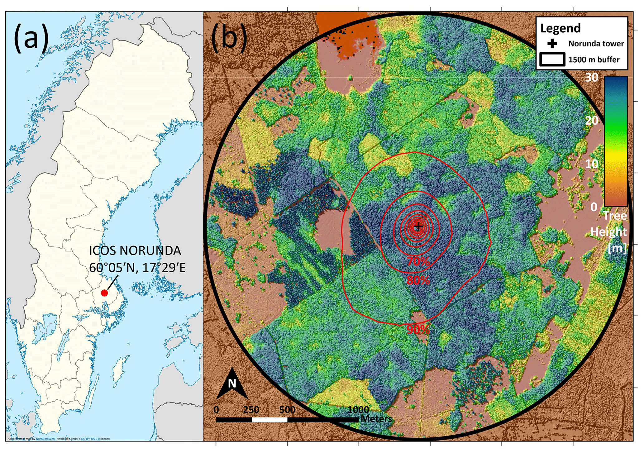
Figure 1 Location of ICOS station Norunda (a) relative to Sweden as a whole. Panel (b) shows the tree height surrounding the station in detail from above (2011) and the footprint of the Norunda tower at 36 m (red contours) for the 2014–2016 campaign period. Contours were calculated using the Flux Footprint Prediction (FFP) footprint model (Kljun et al., 2015). Each contour line adds a 10 % contribution (the contours show 10 % to 90 %). The black cross is the tower location.

In addition to the typical ICOS station standard instrumentation (Rebmann et al., 2018), there are 11 Metek 3D sonic anemometers (USA-1, Metek GmbH, Germany) mounted on the flux tower at heights from 4 to 100.5 m a.g.l. (see Fig. 2). These anemometers are mounted on booms extending 5 m towards north–northwest from the tower.

2.2 Trace gas sampling

Ambient air from six heights (4, 8.5, 13.5, 19, 24.5, and 33.5 m a.g.l.; forest canopy height H=28 m) was pulled down by two vacuum pumps (Vaccubrand ME2, Wertheim, Germany) using six heated and insulated perfluoroalkoxy (PFA) Teflon tubes mounted on the station flux tower (Fig. 2). These sampling tubes were each 45 m in length with an outer diameter (OD) of 3/8 in. The flow rate through each PFA tube was 20 L min⁻¹. Sample air residence time in tower tubing before reaching instrumentation was ca. 4.5 s. The measurements took place during several periods from 2014 to 2016 and were collected by sampling at each height for 5 min consecutively during a 30 min sampling cycle. BVOC measurements were collected from 12 September 2014 to 11 January 2015, from 21 May to 16 December 2015, and from 28 April to 5 July 2016. Ozone measurements were collected using the same sampling cycle from 13 September 2014 to 10 October 2016. A Campbell Scientific (Logan, UT, USA) CR1000 datalogger with an SDM-CD8S switch module was used to control a set of polytetrafluoroethylene (PTFE)-coated solenoid valves (Parker Hannifin, Hollis, NH, USA) to subsample air (total 1 L min⁻¹) from the selected main inlet flow for trace gas analysis.

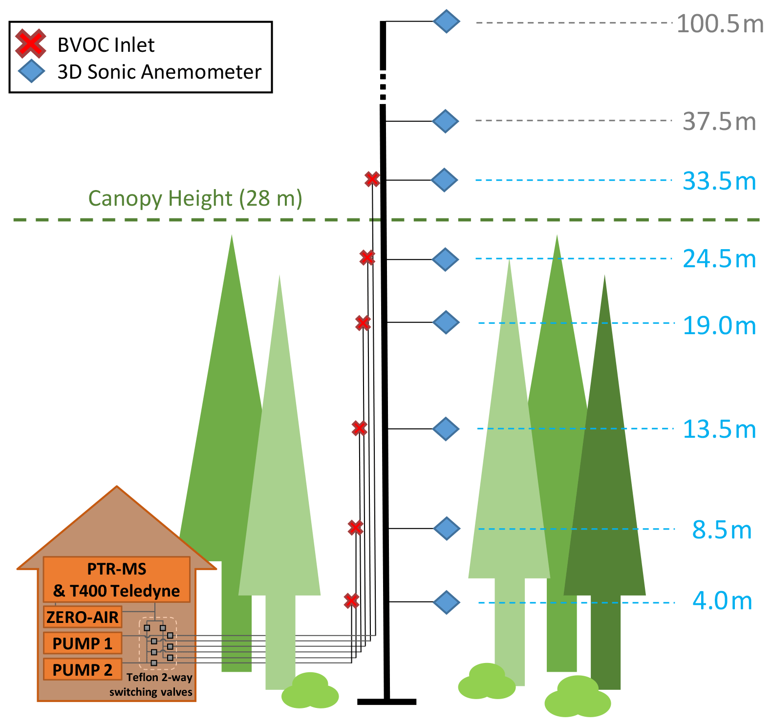
Figure 2 BVOC inlet setup at Norunda. Shown are the heights of the 3D sonic anemometers (blue diamond) and BVOC inlets (red cross) at the station flux tower. The canopy top height is at approximately 28 m. The instrument shed contained the PTR-MS, the Model T400 Teledyne ozone analyzer, a zero-air generator for the PTR-MS, a PTFE valve-switching system, and a pair of vacuum pumps for pulling air through the tower inlet tubing. Two pumps were used to pull air through the tower inlets. Switching every 5 min, pump no. 1 services levels 1, 3, and 5 (33.5, 19, and 8.5 m), while pump no. 2 services levels 2, 4, and 6 (24.5, 13.5, and 4 m). The tower inlet tubes from which sample air was being actively drawn for sampling was therefore pumped, while the tower line for the next 5 min period of the 30 min cycle was pre-pumped.

2.3 Trace gas analysis

Part (0.3 L min⁻¹) of the air subsample flow was analyzed for BVOCs using a proton-transfer-reaction–quadrupole mass spectrometer (HS-PTR-MS, Ionicon Analytik, Innsbruck, Austria). The PTR-MS uses the protonation of compounds by H₃O⁺ ions in a drift tube to ionize the target compounds, with subsequent detection by a mass spectrometer. Compound concentrations were determined using a primary ion H₃O⁺ ($m/z$ 21+) and target ion count rate along with other instrumental parameters following Lindinger et al. (1998) and Holst et al. (2010). For these measurements, the drift tube pressure was set to 2.2 mbar and drift tube temperature was maintained at 60 ^∘C (E / N = 130 Td). The ozone concentrations were measured from the remaining subsample flow (0.7 L min⁻¹) using a UV absorption analyzer (Model T400, Teledyne API, San Diego, CA, USA) in parallel with the BVOC measurements. Reference measurements to determine the instrumental background of the PTR-MS were periodically performed by passing sample air through a heated catalytic converter (Zero Air Generator model 75-83, Parker Balston, Haverhill, MA, USA). Readings of the PTR-MS count rate for target ions were corrected for the mean daily zero-air background values normalized to the count rate of the primary ion 21+ during analysis. During concentration profile analysis, the first and last minutes of each 5 min level were discarded to ensure that sample air was not a mixture of air collected from separate level heights.

The VOCs with related mass-to-charge ratios ($m/z$) selected for measurement using the PTR-MS technique during these field measurements were methanol ($m/z$ 33+), the hexanol fragment ($m/z$ 41+), acetaldehyde ($m/z$ 45+), acetone ($m/z$ 59+), isoprene ($m/z$ 69+), the monoterpenes (primary mass fragments $m/z$ 81+ and $m/z$ 137+), and the parent sesquiterpene ion ($m/z$ 205+). To monitor instrument noise, $m/z$ 25+ (i.e., empty background) was also measured. During the 2016 measurements, the list of VOCs selected for detection by the PTR-MS was extended to include acetic acid ($m/z$ 61+), MVK + MACR ($m/z$ 71+), MEK ($m/z$ 73+), toluene ($m/z$ 93+), the terpene fragment ($m/z$ 95+), and the primary sesquiterpene fragment ($m/z$ 149+). A list of mass-to-charge ratios for which the PTR-MS scanned can be seen in Table 1. The calibration of the PTR-MS was checked using a gravimetrically prepared calibration standard (Ionimed Analytik, Innsbruck, Austria). Instrumental sensitivities for methanol, acetonitrile, acetaldehyde, ethanol, acrolein, acetone, isoprene, crotonaldehyde, 2-butanone, benzene, toluene, o-xylene, chlorobenzene, α-pinene, 1,2-dichlorobenzene, and 1,2,4-trichlorobenzene were determined by multipoint calibration. Additionally, using PTR-MS measurements of the $m/z$ 21+ and 37+ ions (Holst et al., 2010), a comparison was performed between the water vapor readings from PTR-MS observations and station-reported water vapor to check the long-term stability of the PTR-MS system's performance.

Table 1 A list of the $m/z$ ratios scanned by the PTR-MS instrument during the full 2014–2016 field campaign measurements at ICOS Norunda. Compound identification for scanned ions is also provided. The abbreviated compounds are MVK (methyl vinyl ketone), MACR (methacrolein), and MEK (methyl ethyl ketone). Dwell times (s) of the PTR-MS scanning sequences and detection limits (pptv) of the measurements are shown for both the 2014–2015 and 2016 campaign periods. The total PTR-MS scanning cycle durations for the 2014–2015 and 2016 campaign periods were ca. 20 and 24 s, respectively. The detection limit (DL) is the signal-to-noise ratio as determined from a 2× standard deviation of zero-air background measurements (cps) and the sensitivity (cps pptv⁻¹) determined from the campaign-period measurements. The table bottom shows detection limits for the quantified total monoterpene (based on 81+ and 137+ ions) and total sesquiterpene (based on 149+ and 205+ concentrations; pptv).

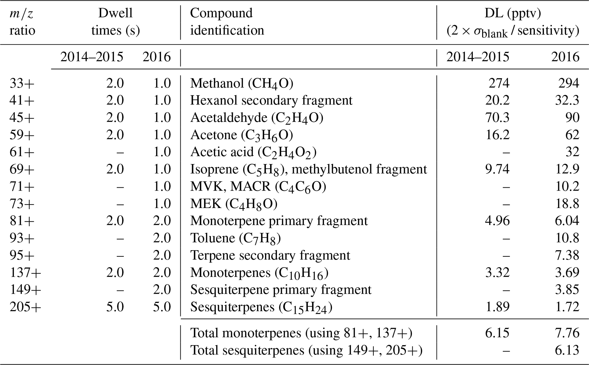
During the 2014–2016 campaign, the PTR-MS was operated with several different measurement sequences as it scanned for different sets of BVOC components. In 2014 and 2015, typical dwell times were 2.0 s, and a typical scanning sequence took about 20 s. In 2016, dwell times were typically either 1 or 2 s, and a scanning sequence took about 24 s. For all the years, the dwell times for the $m/z$ 21+, 25+, 37+, and 205+ ion readings were 0.1, 0.5, 0.1, and 5 s, respectively.

Based on the standard deviation (2σ) of the zero-air background readings of the $m/z$ 21+, 37+, and target ions, the detection limits of the PTR-MS for the VOC concentration measurements (Table 1), and thus the signal-to-noise ($S/N$) ratios, were calculated. For methanol the mean $S/N$ ratio was relatively high (15.4), and the mean $S/N$ ratio for acetone and acetaldehyde was 7.8 and 3.7, respectively. The lowest mean $S/N$ for non-sesquiterpenes was found for isoprene (1.37) at the 95 % confidence level for May to the end of June 2016. The mean $S/N$ ratio for $m/z$ 81+ and 137+ was 9.8 and 7.1, while the mean $S/N$ ratio for total monoterpenes (determined from the 137+ and mass-fragment 81+ readings) was somewhat higher (12.8). The majority (>90 %) of 205+ measurements for all campaign years fell below the detection limit.

Fragmentation of larger BVOC compounds ($>m/z$ 80+) in the PTR-MS is an important consideration (e.g., Steinbacher et al., 2004). Monoterpene concentration is determined from $m/z$ 137+ and its primary fragment $m/z$ 81+ (Steinbacher et al., 2004; Tani et al., 2003). For the 2016 data, an evaluation of the total sesquiterpene concentration was conducted from the concentration of its complete protonated ion ($m/z$ 205+) and its primary fragment ion ($m/z$ 149+). The vast majority of these total sesquiterpene measurements, however, also failed to exceed the calculated detection limit (6.13 pptv). Given that sesquiterpene emissions are ubiquitous in boreal forests during summer, such as at Norunda (e.g., Wang et al., 2017), this indicates that sampled sesquiterpenes were mostly lost to reactions or inlet tubing before the air samples reached the PTR-MS detector.

2.4 Inversion calculations

To quantify the strength of various compound sources and sinks within the forest canopy, Lagrangian dispersion theory was applied.

Unlike previous investigations which relied on empirical (Raupach et al., 1986) or fitted turbulence profiles (Karl et al., 2004) for estimating the standard deviation of the vertical wind speed (σ_w), friction velocity (u_∗), and Lagrangian timescale (T_L), in this analysis we used sonic anemometer measurements from 12 heights to determine the profiles of σ_w, u_∗, and T_L. Sonic anemometer data from these heights were processed according to the methodology presented by Mölder et al. (2004). As Lagrangian timescales T_L cannot be directly measured from one-point measurements (i.e., a sonic anemometer affixed to a stationary tower), T_L values were calculated from measured Eulerian timescale values T_E based on the approach of Raupach (1989), using the relationship

$$\begin{array}{}\text{(1)}& T_{\text{L}}=\mathit{\beta }{\displaystyle \frac{\stackrel{\mathrm{‾}}{u}}{{\mathit{\sigma }}_{\text{w}}}}{T}_{\text{E}},\end{array}$$

where $\stackrel{\mathrm{‾}}{u}$ is the mean wind velocity and β is a scaling constant chosen to be equal to 1 (Raupach et al., 1986). The timescales T_E were defined as the time delay for the autocorrelation function of vertical velocity w to decay to 36.8 % ($\mathrm{1}/e$) of the maximum value (Mölder et al., 2004; Raupach, 1989). The choice of β=1 at and below canopy height has previously been shown to be a reasonable approximation (Mölder et al., 2004; Raupach, 1989). Twelve source layers were used (from 2 m, ca. $z/h=\mathrm{0.07}$, to 100.5 m, ca. $z/h=\mathrm{3.6}$) for the calculation of the source distribution. The six measurement heights for BVOC and ozone were used for interpolation of the concentration gradients at 6.25, 11.0, 16.25, 21.75, and 29.0 m (ca. $z/h=\mathrm{0.22}$, 0.39, 0.58, 0.78, and 1.04). The values of σ_w and T_L at 2 m were described using the parameterization given by Nemitz et al. (2000). Ground-level BVOC emissions are not separated from emissions in this lowest source layer (thickness 2 m) due to the limitations of parameterizing ${\mathit{\sigma }}_{\text{w}}/u_{\ast }$ near the surface (Wilson and Flesch, 1993).

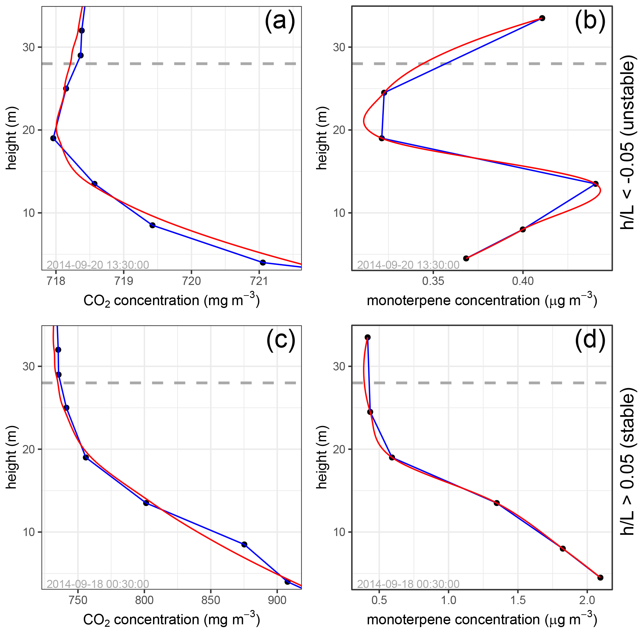
Figure 3 Fitted concentration curves. Panels (a) and (c) show fitted CO₂ profiles. Panels (b) and (d) show fitted monoterpene profiles. Panels (a) and (b) show cases with an unstable, daytime atmosphere, while panels (c) and (d) show cases with stable, nighttime atmospheric conditions. The horizontal dashed line indicates canopy height (28 m).

The ozone and BVOC source or sink distributions in and below the canopy were derived using a Lagrangian dispersion theory approach (Karl et al., 2004; Warland and Thurtell, 2000). In this approach, the source and sink layers in the forest canopy are quantified using dispersion matrix inversion. The dispersion matrix used for analyzing these data utilized the gradient approach formulated by Warland and Thurtell (2000). The dispersion relation is of the form given by

$$\begin{array}{}\text{(2)}& {\displaystyle \frac{\mathrm{d}c}{\mathrm{d}z}}\left|\begin{array}{c}\\ \\ i\end{array}\right.={\sum }_{j=\mathrm{1}}^m{D}_{ij}{S}_j,\end{array}$$

where the concentration gradient at height z_i is the sum of all contributions from source or sink layers S_j at heights z_i. The elements D_ij of the dispersion matrix D are calculated as the sum of near-field and far-field dispersion terms (Eq. A1 in the Appendix). For the BVOC compounds investigated by this analysis, chemical processes such as breakdown or creation of compounds directly in the atmosphere typically occur on timescales much longer than the canopy-mixing timescales used for the Lagrangian dispersion analysis or friction-velocity-based mixing timescales, leading to a quite low Damköhler number (Rinne et al., 2012). Therefore photochemical losses/production are not explicitly parameterized in the inversion analysis procedure and are convoluted with direct sources and sinks.

It is frequently noted that, for Lagrangian dispersion-derived inversions used to calculate source or sink layer strengths, the number of observations should well exceed ($\ge \times \mathrm{2}$) the number of prescribed source or sink layers (e.g., Raupach et al., 1986). This is to improve the robustness of the inversion results. Without this condition, instability is a frequent shortcoming of localized near-field (LNF) and continuous near-field (CNF) models, as noted in Raupach et al. (1986) and Siqueira et al. (2000). To quantify the vertical concentration gradient in the forest canopy using the concentration measurements at the six inlet heights, we fitted a curve to the concentration data (see Fig. 3), and the concentration gradient at heights throughout the canopy was quantified from the slope of the fitted curve. For daytime data, a curve was fitted to the concentration data using a loess fit (Cleveland et al., 1992). The span setting for this loess fit was 0.7. For nighttime data, as concentration gradients tend to be relatively large due to the often stable nighttime atmosphere (see Fig. 3), a concentration curve was established by interpolating between the concentration observations. Figure 3 shows an example of fitted concentration curves for daytime and nighttime monoterpene and CO₂ observations.

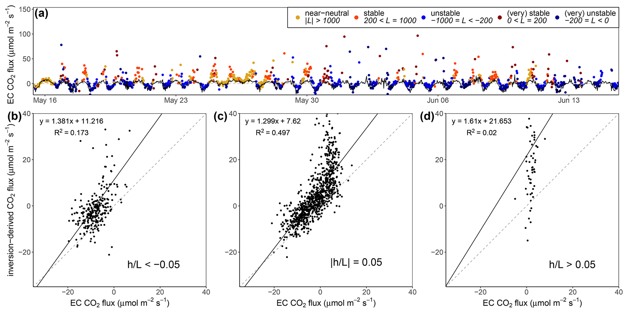
Figure 4 Time series (a) and scatterplots (b–d) showing inferred CO₂ flux from inversions and EC flux measurements. (a) Time series showing measured EC CO₂ flux (black line) and an inversion-derived estimate of CO₂ flux (points). Above-canopy stability conditions at 36 m during flux observations – unstable (blue), near neutral (yellow), and stable (red) – are indicated. The horizontal dashed grey line indicates the zero net flux level. Scatterplots show data points sorted by stability parameter $h/L$ for above-canopy stability conditions at 36 m (b) ($h/L<-\mathrm{0.05}$), (c) ($|h/L|\le \mathrm{0.05}$), and (d) ($h/L>\mathrm{0.05}$). Linear best-fit (black) and R² values for panels (b)–(d) are shown as well.

A damped least-squares approach, weighted by solution smoothness (Siqueira et al., 2000) (Eq. 3), was then applied when performing the inversion, with

$$\begin{array}{}\text{(3)}& {\mathit{S}}^{\text{est}}=\left[{\mathbf{D}}^{\text{T}}\mathbf{D}+{\mathit{ϵ}}^{\mathrm{2}}{\mathbf{W}}_{\text{m}}\right]{\mathbf{D}}^{\text{T}}\left({\displaystyle \frac{\mathit{d}\mathit{c}}{\mathit{d}\mathit{z}}}\right),\end{array}$$

where S^est is the vector of estimated source-layer strengths, D^T is the matrix transpose of D, ϵ is a weighting parameter, W_m is a weighting matrix, and $\mathit{d}\mathit{c}\mathbf{/}\mathit{d}\mathit{z}$ is the vector of vertical gradients of the concentration profile at heights z_i.

The use of this weighted minimization procedure (Menke, 2018) comes from the approach suggested by Siqueira et al. (2000), so that the sensitivity of the inversion to variations in the input measurements is addressed by weighted minimization of both least-squares prediction error and a smoothness measure of the source-layer strengths S_j, as imposed in Eq. (3) by a weighting matrix W_m. The weighting matrix W_m is given by Eq. (4):

$$\begin{array}{}\text{(4)}& \begin{array}{rl}& {\mathbf{W}}_{\text{m}}=\\ & {\left[\begin{array}{cccccc}-\mathrm{1}& \mathrm{1}& \mathrm{0}& \mathrm{\cdots }& \mathrm{\cdots }& \mathrm{0}\\ \mathrm{0}& -\mathrm{1}& \mathrm{1}& \mathrm{0}& \mathrm{\cdots }& \mathrm{0}\\ \mathrm{⋮}& & \mathrm{\ddots }& \mathrm{\ddots }& & \mathrm{⋮}\\ \mathrm{0}& \mathrm{\cdots }& \mathrm{0}& -\mathrm{1}& \mathrm{1}& \mathrm{0}\\ \mathrm{0}& \mathrm{\cdots }& \mathrm{\cdots }& \mathrm{0}& -\mathrm{1}& \mathrm{1}\end{array}\right]}^{\mathrm{T}}\left[\begin{array}{cccccc}-\mathrm{1}& \mathrm{1}& \mathrm{0}& \mathrm{\cdots }& \mathrm{\cdots }& \mathrm{0}\\ \mathrm{0}& -\mathrm{1}& \mathrm{1}& \mathrm{0}& \mathrm{\cdots }& \mathrm{0}\\ \mathrm{⋮}& & \mathrm{\ddots }& \mathrm{\ddots }& & \mathrm{⋮}\\ \mathrm{0}& \mathrm{\cdots }& \mathrm{0}& -\mathrm{1}& \mathrm{1}& \mathrm{0}\\ \mathrm{0}& \mathrm{\cdots }& \mathrm{\cdots }& \mathrm{0}& -\mathrm{1}& \mathrm{1}\end{array}\right].\end{array}\end{array}$$

The choice of the inversion weighting parameter ϵ for the BVOC and ozone inversions was informed by iterating the inversion calculation over a sequence of ϵ values to quantify the CO₂ source- or sink-layer strengths in the Norunda canopy and comparing the modeled CO₂ flux (i.e., the sum of the CO₂ source- or sink-layer strengths in the canopy) to the above-canopy CO₂ flux determined by eddy covariance (at 35 m on the flux tower).

CO₂ mixing-ratio observations were made at heights from 0.8 m to 101.8 m a.g.l. on the Norunda flux tower. Since BVOC measurements were only collected until slightly above the forest canopy ($z/H=\mathrm{1.2}$, up to 33.5 m), only CO₂ gradient fits from 0.8 m up to 33 m on the tower were used for the inversion calculations. Figure 4 shows the results for these CO₂ inversion calculations. It shows that the best CO₂ inversion-derived flux results are typically achieved during near-neutral atmospheric conditions in the canopy and that during stable conditions (predominantly observed at night) the inversions tend to overestimate the magnitude of source- or sink-layer strengths, particularly for positive fluxes out of the forest canopy. Based on the results from comparing inversion-derived to EC-measured CO₂ fluxes, the value of the weighting parameter ϵ for the BVOC and ozone inversions was chosen to be 0.15, based on maximizing the R² value (0.76) of the linear best fit (see Fig. 4). It should be noted that inversion model performance is in general impeded in cases of nonstationarity of atmospheric conditions in the canopy and above, such as during the morning transition from a stable surface layer to the development of the convective boundary layer (e.g., Ouwersloot et al., 2012; Siqueira et al., 2003; Vilà-Guerau De Arellano et al., 2009), when the stationarity assumptions inherent in the formulation of the inversion approach are suspect, e.g., when CO₂ that has built up in the canopy during stable nighttime conditions, i.e., storage, flushes out during the breakup of the stable boundary layer.

3 Results

A range of reactive VOCs and ozone in the ambient air was detected throughout the Norunda canopy. An overview of the daily median values of daily BVOC and ozone concentrations in the forest canopy (35 m) as well as station meteorological measurements during the 2014–2016 field campaign periods can be found in Fig. 5. The 5th-to-95th percentile range of daily BVOC and ozone concentrations at 35 m is shown in Fig. 5 as well. Vertical profiles of turbulence statistics from the sonic anemometer measurements for several seasonal time periods (fall 2014, summer 2015, fall 2015, and spring 2016) are shown in Fig. 6.

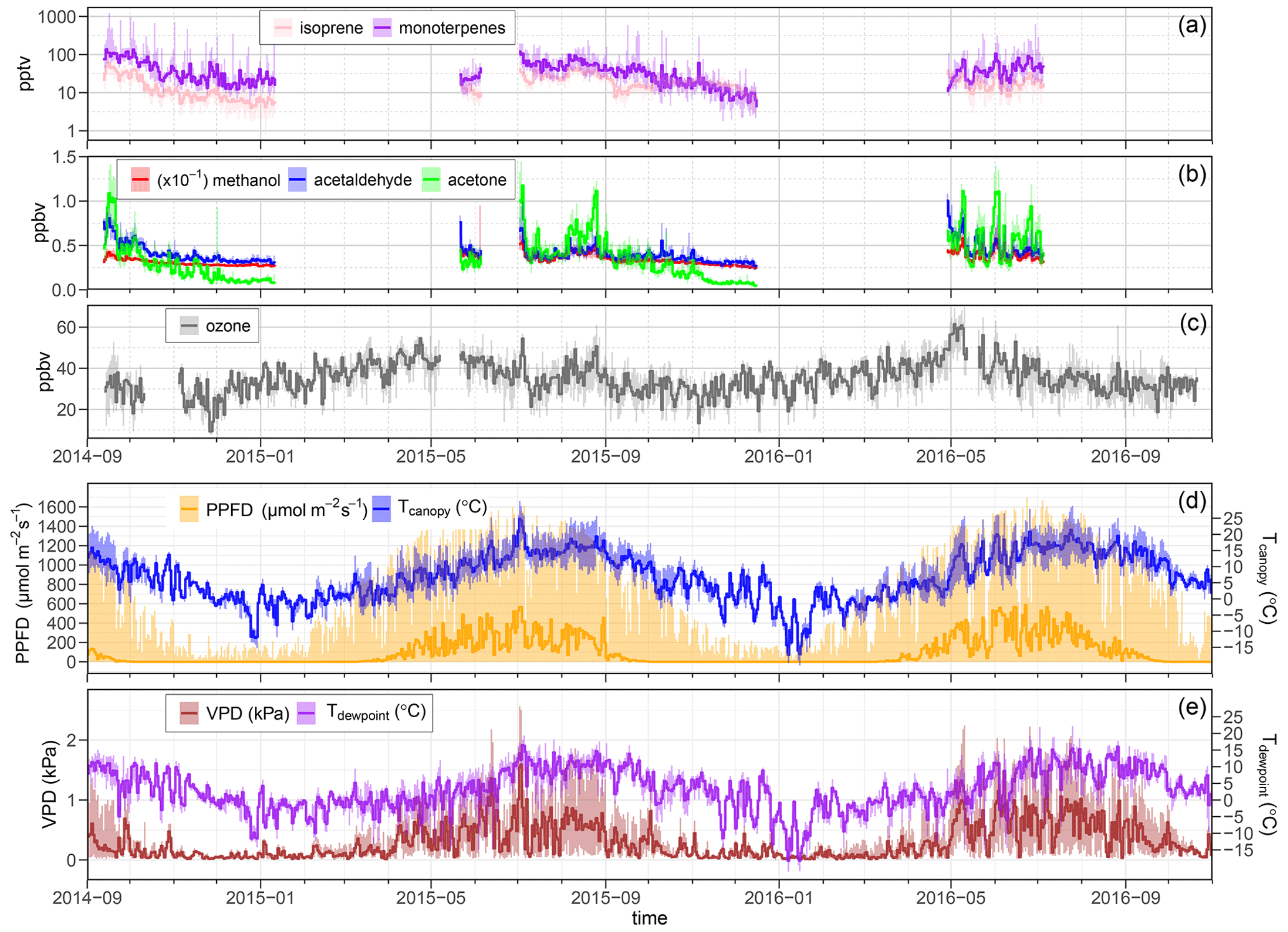
Figure 5 Daily median of the 30 min BVOC concentration (pptv) and ozone concentration (ppbv) sampled at the 33.5 m inlet, as well as related meteorological measurements. The shaded area depicts the 5th-to-95th percentile range of daily concentration. (a) Monoterpene and isoprene concentrations (pptv) shown on a log scale. (b) Methanol ($\times {\mathrm{10}}^{-\mathrm{1}})$, acetaldehyde, and acetone concentrations (ppbv). (c) Ozone concentration (ppbv). (d) PPFD (55 m) and canopy surface temperature (measured by infrared thermometry from 55 m). (b) Vapor pressure deficit and dewpoint temperature (at 36.5 m). Canopy height is 28 m. The set of displayed measurements spans from September 2014 to October 2016.

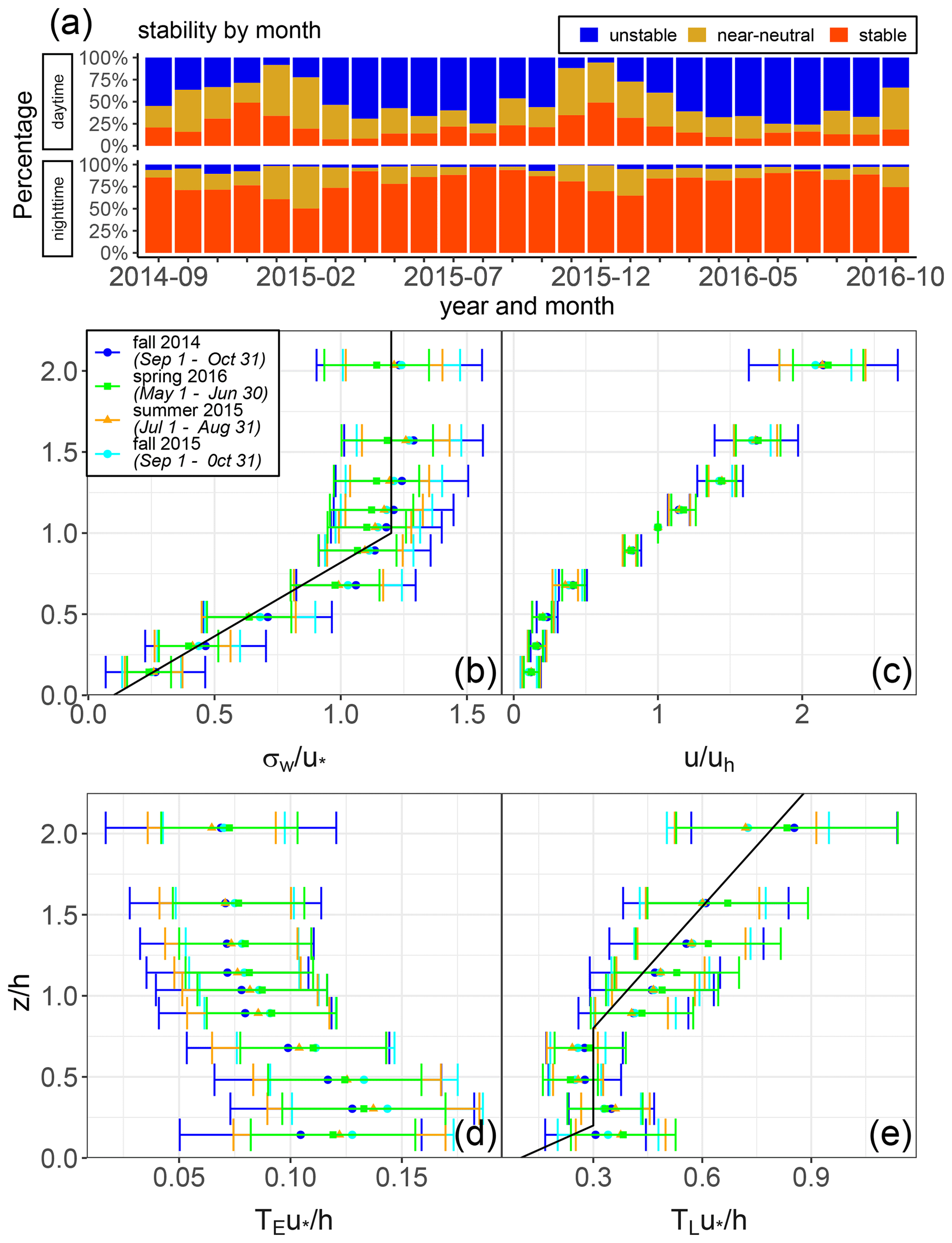
Figure 6 (a) Breakdown of unstable ($-\mathrm{1000}<L<\mathrm{0}$), near-neutral ($\left|L\right|>\mathrm{1000}$), and stable ($\mathrm{0}\le L<\mathrm{1000}$) conditions in the canopy. (b) Vertical profiles for near-neutral conditions of normalized (b) standard deviation of vertical wind velocity σ_w/u_∗, (c) mean wind velocity $U/U_h$ (U_h is the velocity at canopy height), (d) Eulerian timescale $T_{\text{E}}{u}_{\ast }/h$, and (e) Lagrangian timescale $T_{\text{L}}{u}_{\ast }/h$. The black lines, showing empirical fits of normalized σ_w and T_L, are adapted from Mölder et al. (2004). The u_∗ used to normalize the profiles is measured at the top of the tower (100.5 m). On the x axis of these profiles is shown the normalized height $z/h$, where canopy height h is 28 m. Points are determined from 30 min-averaged data, and the standard deviations of these points are plotted as error bars. Data values are shown for fall 2014 and 2015 (dark blue and light blue) for 1 September to 31 October, summer 2015 (orange) for 1 July to 31 August, and spring 2016 (green) for 1 May to 30 June. During the fall 2014 period, there were 664 (23.1 %) unstable, 744 (25.9 %) near-neutral, and 1469 (51.1  %) stable data points. During summer 2015, there were 1191 (42.2 %) unstable, 311 (11 %) near-neutral, and 1319 (46.8 %) stable data points. During the fall 2015 period, there were 647 (24.4 %) unstable, 375 (14.1 %) near-neutral, and 1633 (61.5 %) stable data points. During the spring 2016 period, there were 1393 (48.6 %) unstable, 450 (15.7 %) near-neutral, and 1025 (35.7 %) stable data points.

3.1 BVOC and ozone observations

During the growing season, methanol was detected in the range of 3.0 to 5.1 ppbv throughout the canopy. Peak concentrations in the canopy were typically observed during nighttime under stable atmospheric conditions. Isoprene concentrations were observed to be low in the seasonal observations (e.g., approximately 250 pptv maximum concentration during summer 2015). Given previous branch-level measurements (Wang et al., 2017), this indicates that there is no particularly strong source of isoprene in the forest canopy. Daily median ozone concentrations (at 33.5 m) for the full measurement campaign can also be seen in Fig. 5. In most cases, ozone concentrations ranged from 30 to 60 ppbv during the growing season, with peak concentrations observed above the canopy during the afternoon and minima observed near the forest floor at or near sunrise (Fig. 7).

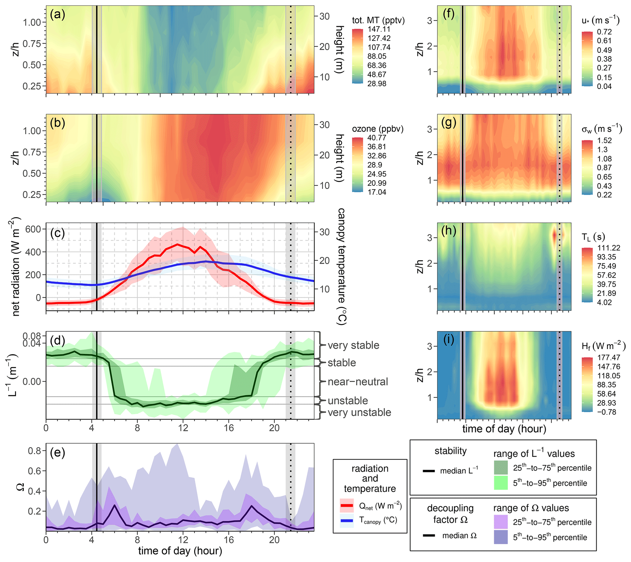
Figure 7 Mean diurnal cycle of (a) monoterpene and (b) ozone profile concentrations for a clear-weather period of summer 2015 (20 July to 10 August). (c) Net radiation (red) and canopy temperature (blue). Net radiation and canopy temperature are measured at 55 m. Shaded regions of net radiation and canopy temperature indicate 1 standard deviation. (d) Plot of the inverse of the Obukhov length (L⁻¹), indicating the atmospheric stability above the canopy (measured at 36 m). Classification of stability from Obukhov length (L) values (very stable: $\mathrm{0}\le L<\mathrm{200}$, stable: $\mathrm{200}\le L<\mathrm{1000}$, near-neutral: $\mathrm{1000}\le \left|L\right|$, unstable: $-\mathrm{1000}<L\le -\mathrm{200}$, very unstable: $-\mathrm{200}<L\le \mathrm{0}$). (e) Plot of the decoupling factor Ω, indicating the degree of aerodynamic coupling between canopy vegetation and the atmosphere above the forest canopy. See the Appendix for more details regarding Ω. (f) Diurnal mean contour profiles of friction velocity u_∗ (m s⁻¹), (g) standard deviation in vertical wind velocity σ_w (m s⁻¹), (h) Lagrangian timescale (s), and (i) sensible heat flux H_f (W m⁻²) with respect to the normalized height $z/h$ in the forest. In all the panels, sunrise (solid vertical line) and sunset (dotted vertical line) are indicated. The shaded region indicates the range of sunrise and sunset times during the 20 July to 10 August period.

3.1.1 Isoprenoids

Typically for a forest with a tree species composition such as Norunda, isoprene concentrations peak in the summer months. Isoprene concentrations were below 20 pptv in the fall, less than 5 % of the time concentrations exceeded 35 pptv, and the mean concentration was 20 pptv. The maximum value occurred during daylight hours at a time when temperature and photosynthetic photon flux density (PPFD) were high (>20 ^∘C and >1000 µmol m⁻² s⁻¹) as well, with concentrations falling to daily lows at all measurement heights towards the evening. The inversion results for isoprene are also consistent with its emission being light-dependent, with the source profiles indicating there being an albeit weak canopy source during the day. As expected, little to no isoprene emission was observed at night. The nighttime inversion profile (known to be biased toward overpredicting source strengths due to nighttime conditions, e.g., Siqueira et al., 2002, 2000) shows negligible source-layer strength for isoprene during nighttime hours from 15 July to 15 August 2015 (<0.3 ng m⁻² s⁻¹ per level, with 0.64 ng m⁻² s⁻¹ for total inferred flux out of the canopy).

Like isoprene, monoterpene concentrations at Norunda were typically highest in the summer months. Peak monoterpene concentrations (1–1.4 ppbv) in the canopy were an order of magnitude higher than isoprene concentrations. Monoterpene concentrations near the forest floor peaked during the night, while monoterpene concentrations in and above the canopy level typically peaked during or shortly following sunrise. An example showing the morning concentration behavior of monoterpenes is shown in Fig. 7. This can be due partly to the delay between sunrise (with increasing temperatures) and the development of a well-mixed boundary layer through the stable nocturnal boundary layer.

3.1.2 Water-soluble BVOCs

The summertime high methanol concentration was typically observed in August, with a median concentration of 4 ppb being observed in August 2015 (see Fig. 5). Within the canopy, there was a noticeable decrease in concentrations from mid-May to June. Inversion results (see Sect. 3.3) indicate that this was likely due to strong sinks in the canopy. The highest methanol concentrations were also typically observed in spring, with a median concentration of 4.4 ppb being observed in mid-April 2016. Median methanol concentrations of 4.1 and 4.2 ppbv were observed in May 2015 and 2016, respectively. Acetaldehyde exhibited a similarly high springtime concentration tendency to methanol. Acetone had a minimum concentration in the fall and a peak concentration in August. From August, acetone concentrations above and within the canopy decreased markedly with the progression of fall, to a greater degree percentage-wise than the other PTR-MS-measured compounds.

3.1.3 Other VOCs (2016 observations)

From the 2016 data, toluene concentrations were found to be generally low during daytime (ca. 15 pptv) and increased during nighttime (up to 60 pptv). This is consistent with the buildup of evenly distributed anthropogenic background emissions during night into the shallow nocturnal boundary layer (Karl et al., 2004). Similar behavior was found for $m/z$ 95+, which typically had a daytime low concentration (9 pptv) and a maximum during nighttime (ca. 40 pptv).

During spring 2016, acetic acid concentrations tended to be at a minimum following sunrise (60 pptv) and gradually increased throughout the day until peaking before sunset (ca. 150 pptv), at which point concentrations typically decreased until the next sunrise. The exception to this trend appears to be when there was a persistent high nighttime concentration in the canopy, which was associated with similar peaks in acetone, acetaldehyde, and methanol concentrations in the canopy. Unlike many other compounds, the acetic acid concentrations in the forest canopy were higher in the first 2 weeks of May than in the last 2 weeks of June. The diurnal concentration of $m/z$ 41+, associated with the PTR-MS protonation process as a hexanol fragment, typically followed a similar pattern to acetone. The minimum in the $m/z$ 41+ concentration (about 50 pptv) typically occurred on the morning following sunrise. Concentrations then usually peaked after sunset (about 130 pptv).

For May to June 2016, the mean MVK + MACR concentration was 12 pptv. For June to July 2016, the mean MVK + MACR concentration increased to 19 pptv. From the 2016 measurements, we can estimate the photochemical loss from the ratio of isoprene to MVK + MACR if we assume turbulent exchange times of approximately 50–110 s during daytime, with this timescale based on the far-field limit of Lagrangian dispersion, ${\mathit{\sigma }}_z=\sqrt{\mathrm{2}{\mathit{\sigma }}_{\text{w}}{T}_{\text{L}}\left(t-T_{\text{L}}\right)}$ (e.g., Raupach, 1989). For this summer period, following the approach of Karl et al. (2004), it was estimated that less than 10 % of isoprene was oxidized within the canopy. Figure 8 shows the isoprene : MVK-MACR ratios for the 2016 measurements. The range of observed MEK concentrations was 30–150 pptv and was comparable to those reported by Ruuskanen et al. (2009) for a similar boreal forest site.

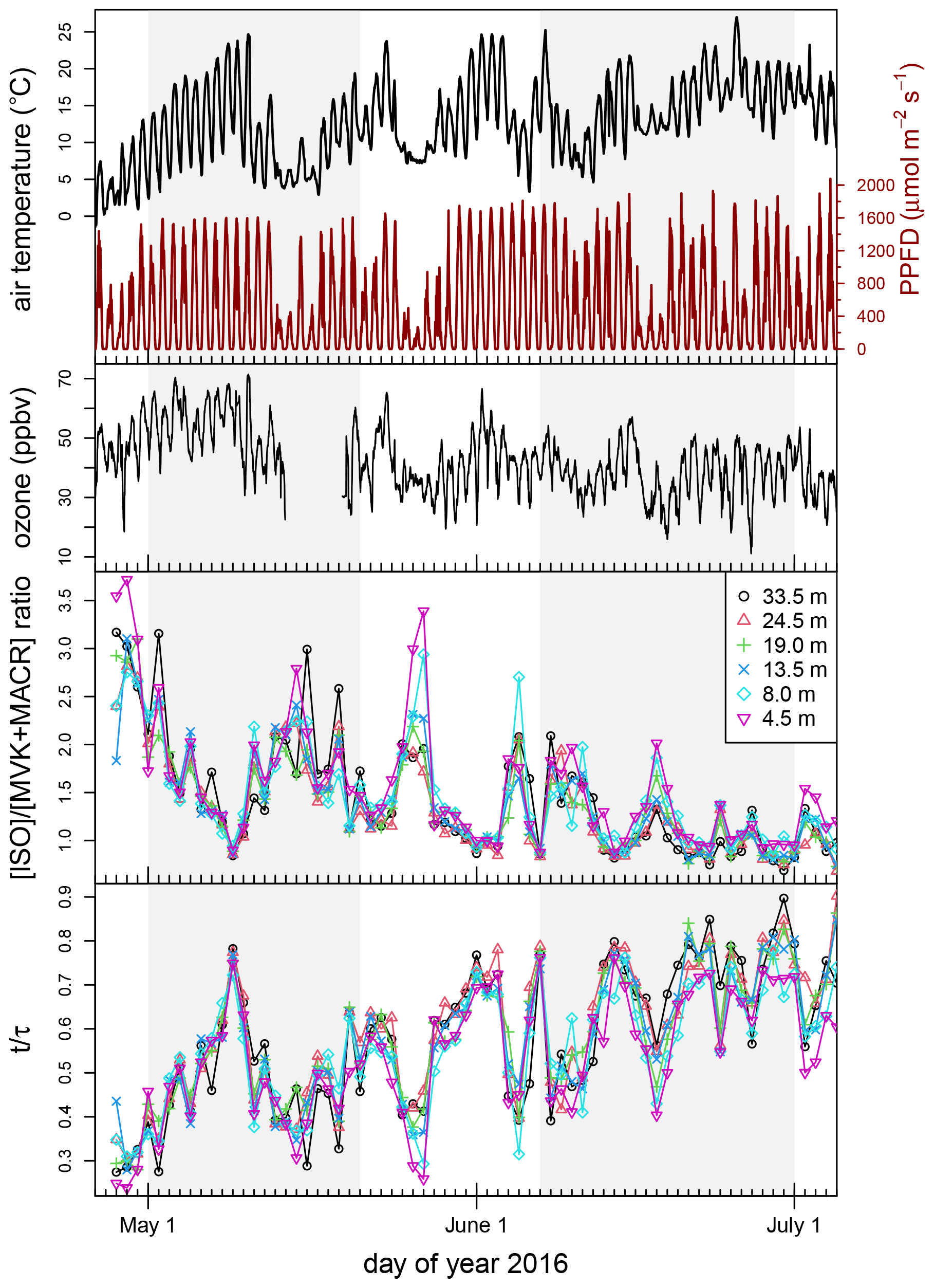
Figure 8 Daytime ratio of isoprene to MVK + MACR from 1 May to 1 July 2016. The (top panel) air temperature (^∘C) (black), PPFD (µmol m⁻² s⁻¹) (red), and ozone (ppbv) (black), (middle panel) the ratio of isoprene to the oxidation products MVK and MACR, and (bottom panel) the ratio of time t progressed to time constant τ vs. day of year. Air temperature and PPFD displayed were measured at 35 m and ozone at 33.5 m. The two shaded areas indicate the two seasonal time periods presented in Fig. 10.

3.2 Source or sink inversion results

The seasonal average source and sink distributions for isoprene, monoterpenes, methanol, acetaldehyde, and acetone are plotted in Fig. 9. For summer 2015, the average inversion-derived isoprene daytime flux for the 4-week period shown in Fig. 9 was 7.3 µg m⁻² h⁻¹. The highest emissions of monoterpene occurred during summer in the upper part of the canopy (at approximately 25 m). The average inversion-derived daytime monoterpene flux for this 4-week period was 120 µg m⁻² h⁻¹ (±30.3 µg m⁻² h⁻¹), with a source strength of up to 9.7 ng m⁻² s⁻¹ per level (±34.6 µg m⁻² h⁻¹ per level) found in the middle canopy (i.e., the layer from 19 to 25 m). These values are consistent with strong monoterpene (MT) emissions previously reported at ICOS Norunda during this seasonal time period (Wang et al., 2017).

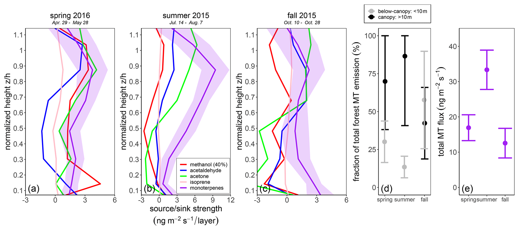
Figure 9 Seasonal BVOC inversion results for the canopy source and sink profile distribution. (a–c) Data shown represent the average of daytime concentrations (from 1.5 h after sunrise to 1.5 h before sunset) for (a) summer 2015, 14 July to 7 August, (b) fall 2015, 1 to 28 October, and (c) spring 2016, 29 April to 28 May. The shaded region for monoterpenes indicates ± standard error. (d) Relative contribution to total monoterpene emission from the canopy (black) and from below canopy (gray) and (e) total inferred monoterpene flux (purple) for the spring 2016, summer 2015, and fall 2015 periods shown in panels (a–c).

The relative seasonal contribution from the canopy and below the canopy to total forest MT emissions in spring, summer, and fall was quantified from the daytime source profiles presented in Fig. 9. The uncertainty range for the percentage relative contribution to the total inferred MT flux from the canopy and below the canopy was quantified by standard error propagation. During summer 2015, for the total-inversion-derived daytime MT flux of 120 µg m⁻² h⁻¹, an average of 86.4 % originated from the canopy and 13.6 % from below the canopy. During fall 2015, for an inferred daytime MT flux of 45.2 µg m⁻² h⁻¹ (±17.6 µg m⁻² h⁻¹), an average of 42.3 % came from the canopy and 57.7 % from below the canopy. During spring 2016, for a total-inversion-derived daytime MT flux of 60.9 µg m⁻² h⁻¹ (±18.44 µg m⁻² h⁻¹), an average of 69.9 % came from the canopy and 30.1 % from below the canopy.

The 2016 BVOC inversion results for two spring and early-summer periods (1 to 24 May and 7 June to 1 July, respectively) for the canopy source and sink profile distributions are shown in Fig. 10, showing how the inversion-derived distribution of sources and sinks evolved from the spring to summer growing seasons for the expanded list of VOC compounds that were monitored during this period. For this 2016 period, the typical daytime inversion-derived ozone flux was found to vary between approximately −0.3 and −0.9 µg m⁻² s⁻¹. From this ozone flux, we derive an ozone deposition velocity that varies between approximately 0.4 and 0.9 cm s⁻¹.

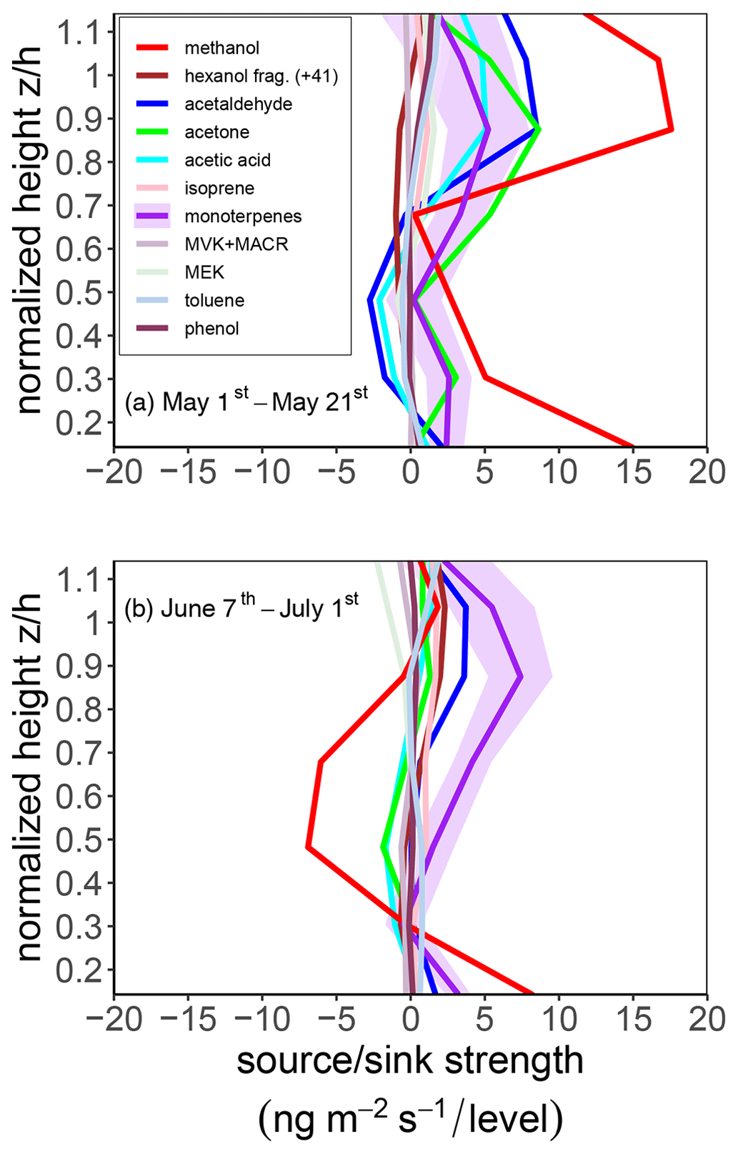
Figure 10 2016 BVOC inversion results for the canopy source and sink profile distribution. Data shown represent the average of daytime concentrations (from 1.5 h after sunrise to 1.5 h before sunset) for (top panel) 1 to 21 May and (bottom panel) 7 June to 1 July 2016. The shaded region for monoterpenes indicates ± standard error. The flux tower air temperature and PAR during these time periods are shown in the top panel of Fig. 8.

While daytime concentrations for methanol, acetaldehyde, and acetone often followed a predictable behavior for a particular season, it was observed that the relative nighttime concentration patterns could be quite variable, particularly at a seasonal scale between the fall, spring, and summer seasons. An example of this variability is presented in Fig. 11. Strong enhancement of nighttime sinks of water-soluble BVOC compounds (i.e., methanol, acetaldehyde, and acetone) is noted to frequently coincide with the presence of favorable dew-forming conditions in the forest canopy.

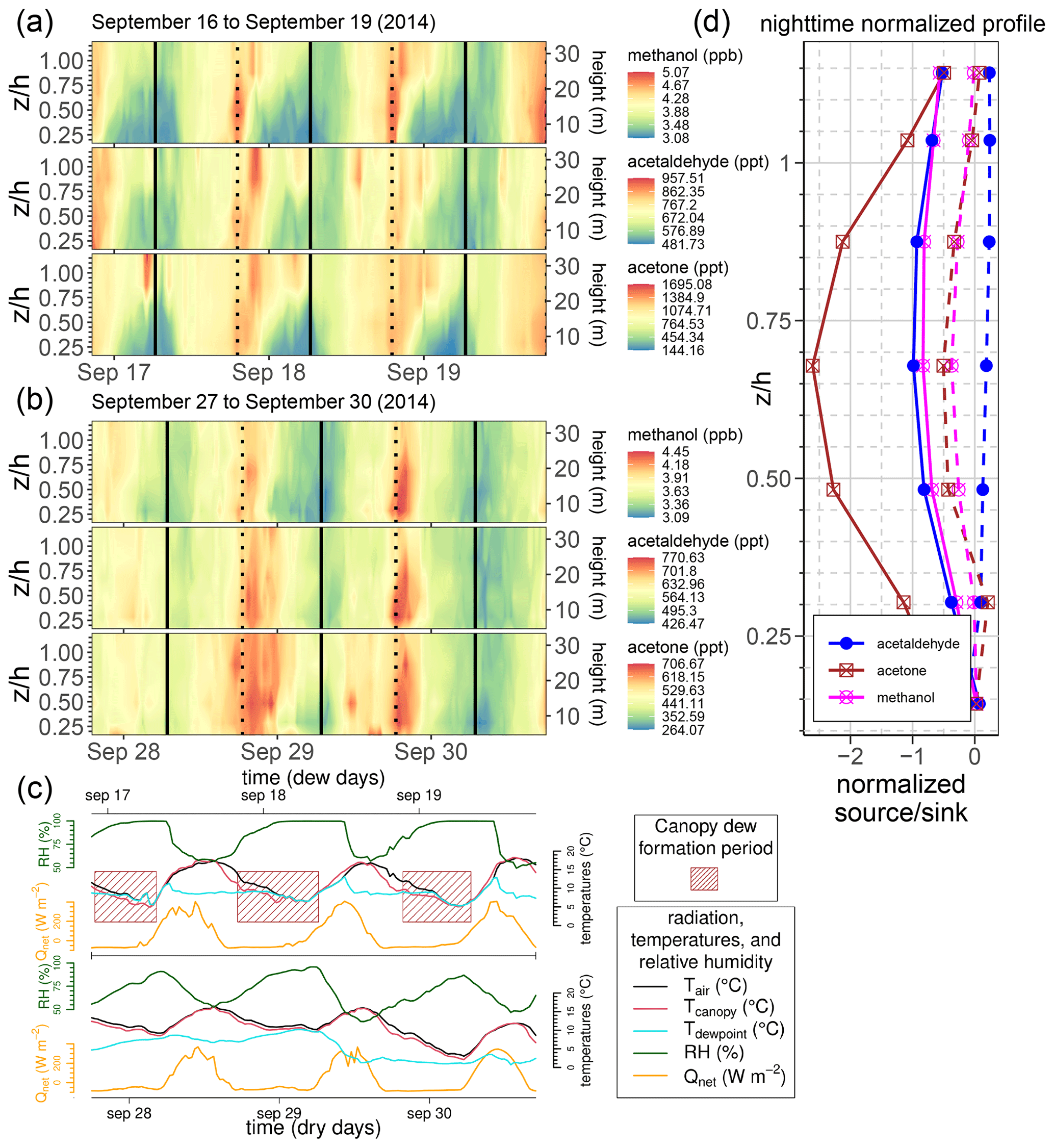
Figure 11 Nighttime dew effects on water-soluble BVOCs in the forest canopy. (a) Methanol concentration profile from 16 to 19 September during conditions where nighttime dew is assumed to have formed in the forest canopy. (b) Methanol concentration profile 2 weeks later, from 27 to 30 September, during dry conditions. In panels (a) and (b), sunrise (solid vertical line) and sunset (dotted vertical line) are indicated. (c) 3 d time series for meteorological conditions during the “dry” period from 27 to 30 September (bottom of the panel) and during the “dew” periods from 16 to 19 September (top of the panel). The meteorological values shown are air temperature (black) in the canopy (at 28 m), IR-measured canopy surface temperature (red), dewpoint temperature (cyan) in the canopy (at 28 m), relative humidity (green), and net radiation (orange). Relative humidity is measured at 28 m. Time periods when dew is expected to have formed in the forest canopy during the dew periods are indicated in panel (c) with brown boxes. (d) Normalized source and sink profiles, for methanol, acetaldehyde, and acetone, during the dew and dry periods. Both the left- and right-panel profiles are normalized by the sum of the dry-period profile-level strengths.

4 Discussion

The isoprene inversion results show a clear diurnal behavior for isoprene emission. The range of observed isoprene concentrations, while relatively low, is consistent with a spruce and pine boreal forest (e.g., Hakola et al., 2017; Rinne et al., 2005) such as Norunda and with values previously reported at the station (Wang et al., 2017).

A local maximum in MT concentrations is frequently observed to occur just prior to, during, or just after sunrise (for example, see Fig. 7). This can take place due to a combination of factors, primarily the rise in the needle temperature following sunrise, followed later by the morning onset of hydrostatic instability in the canopy. For example, there was frequently a change in canopy turbulence profile occurring around the same time as sunrise, with the profile switching from stable or highly stable to unstable or highly unstable as characterized by the Obukhov length L. This was coincident or immediately following in time with the rise in canopy temperature and net radiation occurring with sunrise. The same phenomena are well known from previous studies of forest CO₂ concentrations (e.g., Aubinet et al., 2012). Diurnal changes in plant needle physiology would not seem to contribute much to this occasional morning burst behavior. Niinemets and Reichstein (2003) rule out stomata as effectively controlling the emission rates of VOC compounds, with a Henry's law constant exceeding approximately 100 Pa m³ mol⁻¹. Given typical values of Henry's law constant for monoterpenes, from approximately 2615 Pa m³ mol⁻¹ for γ-terpinene to 13 560 Pa m³ mol⁻¹ for α-pinene (Copolovici and Niinemets, 2005), this would seem to rule out a stomatal-controlled morning burst in monoterpene emissions.

Scaling up the seasonal inversion results, for the 2015 to 2016 measurements (May through October), the average daytime flux per square kilometer of forest during the growing season for isoprene and monoterpenes is estimated to be approximately 205 and 1803 g km⁻² d⁻¹ (ca. 9 and 75 µg m⁻² h⁻¹). Within a few percentage points, these values are consistent with the summer terpene mass fractions (6 % isoprene and 65 % monoterpenes) previously reported at Norunda by Wang et al. (2017).

The monoterpene emission from the canopy relative to below the canopy increased (by ca. 70 % to 86 % from the canopy) from spring to summer. In fall, meanwhile, emissions from the canopy and below the canopy were of a similar magnitude (ca. 42 % vs. 58 %, respectively). Past studies have shown that needle litter in boreal forests can be a prominent contributor to BVOC emissions in fall, particularly for monoterpenes (Aaltonen et al., 2011; Kainulainen and Holopainen, 2002). The same is true for enhanced fall emissions of monoterpenes observed in boreal forests due to soil microbial activity (Mäki et al., 2019b). It is possible that litter deposited the previous year may also have contributed in part to the relatively closer fraction in springtime (ca. 30 % vs. 70 % compared to 14 % vs. 86 % in summer 2015) found earlier in the growing season, as a large portion of the forest needle litter may not have decomposed or been released from needle storage as efficiently, due to decreasing temperatures in fall and winter, until the following spring (e.g., Aaltonen et al., 2011; Wang et al., 2018).

Of all the BVOC compounds observed, methanol has perhaps the most variable distribution of sources and sinks in the canopy at a seasonal timescale. The methanol source profiles derived by the Lagrangian inversions featured strong increases in canopy methanol sources during late April to early May, corresponding in time to new spring growth and conifer budding at the start of the growing season. Methanol production is strongly associated with plant tissue growth (such as during spring and nighttime growth), particularly pectin demethylation in cell-wall-formation processes (Galbally and Kirstine, 2002; Hüve et al., 2007; Macdonald and Fall, 1993b).

In both 2015 and 2016, while there were no substantial methanol sources inferred from the Lagrangian inversions just below the main bulk of the canopy (25 m) during this seasonal period, there was also a large source (lowest source layer at 4 m) near the forest floor. For the spring growing season, if the 4 m layer source is taken as indicative of fluxes from the forest floor, then the inversion-inferred springtime methanol emissions from and just above the forest floor at Norunda are on par with the weekly mean surface methanol emissions observed at other boreal forest sites (Mäki et al., 2019a). Likewise, as observed by long-term surface chamber measurements in Mäki et al. (2019a), the bulk of forest floor VOC exchange inferred from the Lagrangian inversion model appears to be predominantly monoterpenes and methanol.

Meanwhile, another frequent feature that was present in the Lagrangian inversion results was the episodic enhancement of nighttime canopy sinks of methanol, acetone, and acetaldehyde. It is well known that dew can play a role in the deposition of reactive trace gases to wet surfaces (e.g., Chameides, 1987; Karl et al., 2004; Zhou et al., 2017; Wohlfahrt et al., 2015). For the 2014–2016 campaign measurements of methanol and other compounds like acetone and acetaldehyde, it was clear in the inversion results that, for the majority of nighttime periods in summer and fall when the conditions for dew to form on canopy surfaces were present, a strong enhancement of sink behavior manifested in the forest canopy as well. The fact that these sink enhancements occur in the nighttime inversion observations for water-soluble BVOCs but did not for compounds with a large Henry's law constant like isoprene and the monoterpenes further shows that this is a dew-deposition-related effect. Acetone and acetaldehyde featured similar nighttime sink behavior to methanol in the Lagrangian inversion results when dew was present on canopy surfaces, but not at the same magnitude as methanol. This observation is consistent with the Henry's law constant values of methanol, acetone, and acetaldehyde, as the value is an order of magnitude lower for methanol than the other two compounds (e.g., Niinemets and Reichstein, 2003).

Even though daytime net fluxes of acetone and acetaldehyde tend to be quite similar, the observed pattern of source and sink layers in the forest canopy, i.e., the distribution of layers, tended to be very different. Our spring and summer source profiles indicated that the distribution of acetone sources tapered more sharply approaching the canopy top than it did for acetaldehyde, which tended to have had strong sources high to midway up the canopy (top three source layers), followed by a weak sink below the main canopy (13.5 and 8.5 m layers) and a source near the surface (4 m layer).

Previous studies have also considered the canopy distribution of acetone and acetaldehyde sources. For example, with cuvette measurements, Cojocariu et al. (2004) observed smoothly declining acetaldehyde emissions from the top to the bottom of a spruce forest canopy, while for a tropical forest, Karl et al. (2004) found, for a strong source maximum at the very top of the canopy crown, a sink in the lower part of the crown and a source region corresponding to the understory.

Two known pathways for acetaldehyde emission are the conversion of cytosolic pyruvate and the oxidation of ethanol (Cojocariu et al., 2004; Kreuzwieser et al., 1999). The cytosolic pyruvate path is associated with the accumulation of pyruvate in the plant cell cytosol and subsequent burst in pyruvate decarbonxylase reactions (Karl et al., 2002) consistently observed in laboratory studies during light–dark transitions (e.g., Kreuzwieser et al., 2000). The ethanol oxidation path can cause acetaldehyde emission in leaves (e.g., Kreuzwieser et al., 2000, 1999). The production of ethanol is associated with hypoxic or anoxic conditions occurring in the roots (Kreuzwieser et al., 2000) and transport of ethanol through the xylem to leaves and needles, where it can be released through stomata. Compared to acetaldehyde, relatively little experimental information is available on the production and emission pathways for acetone. It has been previously hypothesized that acetone is produced in spruce needles by acetoacetate decarboxylation (Macdonald and Fall, 1993a). Afternoon concentration increased in the relatively longer-lived compounds acetaldehyde, acetone, and methanol. These increases occurred from around mid-afternoon to before sunset (see Fig. 11) and were most likely due to decreased turbulence and the formation of a stable nocturnal boundary layer (e.g., Karl et al., 2004).

As with the Karl et al. (2004) investigation, albeit in a boreal rather than tropical setting, we attribute our acetaldehyde source distribution to reflect a combination of the two known acetaldehyde emission pathways, with a light-induced increase in overall acetaldehyde emission due to the pyruvate pathway (i.e., alternating light–dark shading conditions) higher up in the forest canopy. Interestingly, in 2016, when acetic acid was measured, high canopy concentrations of acetic acid early in the day seemed to presage strong peaks in other compounds monitored in the afternoon and evening. The canopy often appeared to be a sink of acetic acid from the atmosphere, but during days with increased metabolic activity in the forest canopy (temperature >25 ^∘C, PPFD near saturation), the forest also appeared to be a source of acetic acid during daytime and often later the following night. It is known that production and use of acetic acid in plants are linked to metabolism and biosynthesis activity via the hydrolysis and reactivation of the intermediate acetyl-CoA (e.g., Liedvogel and Stumpf, 1982). Another source of acetic acid in plants, linked to the production of acetaldehyde, is the pyruvate dehydrogenase pathway, whereby pyruvate is decarboxylated to acetaldehyde, which is then oxidized to acetic acid (e.g., Jardine et al., 2010). During daytime, the forest appeared to be in general a net sink of acetic acid (see Fig. 10). It would be of interest in future studies to investigate the emission of acetic acid from the Norunda forest or similar boreal forests during the fall season, when other ecosystem processes, such as senescence, might be expected to be taking place.

5 Conclusions

In this study, vertical profiles of BVOC, ozone, and turbulence parameters were measured in a boreal forest canopy during several seasonal periods from 2014 to 2016, providing new insight into BVOC exchange processes in boreal forest. A Lagrangian dispersion methodology was developed to investigate the distribution of BVOC and ozone sources and sinks in the Norunda boreal forest canopy. Our results show complex seasonal behavior in source and sink characteristics for BVOCs within this forest canopy, indicating that further investigations seeking additional insight of BVOC emission and deposition properties within boreal forest ecosystems is warranted.

From the Lagrangian dispersion analysis, the monoterpene source strength was found to typically peak mid-canopy (approximately 25 m), while we observed a strong source near the surface (4 m layer) during the fall. The monoterpene emission from the canopy relative to below the canopy increased (by ca. 70 % to 86 % from the canopy) from spring to summer, while in fall, emissions from the canopy and below the canopy were found to be similar in magnitude. The increased relative emissions from below the canopy are attributed to increased understory litter and soil emissions during the fall (Wang et al., 2018).

Relatively low levels of isoprene (summer mean approximately 25 pptv) were observed in the canopy. As the forest is predominantly composed of Norway spruce and Scots pine, known to be low/no emitters of isoprene, this is consistent with the composition of the forest and previous isoprenoid measurements at Norunda (Wang et al., 2017).

An enhancement in canopy and understory methanol sources was observed in the Lagrangian inversion results during the spring growing season and attributed to increased methanol production and emission by new growth. Strong episodic nighttime enhancement of nighttime sinks of methanol and other water-soluble BVOCs was noted in the summer and fall periods and was most likely associated with deposition to wet surfaces due to the formation of nighttime dew in the canopy. Both the concentration profile and the inversion results for ozone indicate that the canopy is a significant daytime ozone sink. This likely produces a vertical canopy gradient for the photochemical lifetimes of short-lived (1–20 s) BVOC compounds, such as sesquiterpenes.

While it is generally evident that eddy covariance (or often other surface-layer flux measurement approaches (e.g., Rantala et al., 2014) for that matter) provides greater quantitative resolution in determining ecosystem fluxes than any inverse Lagrangian dispersion approach, the application of inverse Lagrangian modeling to BVOC canopy profile measurements nonetheless fulfills a clear and useful role in filling the gap between bottom-up (e.g., branch-level emissions) and top-down (e.g., ecosystem-scale flux) measurements for BVOC emission studies in boreal forest ecosystems. A specific understanding of gas-phase processes within the forest canopy and the species-resolved source or sink strength distribution of a forest region (Roldin et al., 2019; Thomsen et al., 2021) is important for assessing, e.g., the impact of boreal ecosystems on the formation of secondary organic aerosols (SOA) and their impact on the regional radiative forcing (Paasonen et al., 2013).

Appendix A

$$\begin{array}{}\text{(A1)}& \begin{array}{rl}{D}_{ij}& =\left\{{\displaystyle \frac{-\left[\mathrm{1}-\text{exp}\left(\frac{-{\left(z_i-z_j\right)}^{\mathrm{2}}}{\mathrm{2}\mathrm{\Delta }{z}_j^{\mathrm{2}}}\right)\right]}{\mathrm{2}{\mathit{\sigma }}_{\text{w}}^{\mathrm{2}}\left(z_i\right)\cdot T_{\text{L}}\left(z_i\right)\cdot \left[\mathrm{1}-\text{exp}\left(-\sqrt{\frac{\mathit{\pi }}{\mathrm{2}}}\frac{\left(z_i-z_j\right)}{\frac{\left[{\mathit{\sigma }}_{\text{w}}\left(z_i\right)\cdot T_{\text{L}}\left(z_i\right)+{\mathit{\sigma }}_{\text{w}}\left(z_j\right)\cdot T_{\text{L}}\left(z_j\right)\right]}{\mathrm{2}}}\right)\right]}}\right.\\ & \left.-{\displaystyle \frac{\left[\mathrm{1}-\text{exp}\left(\frac{-{\left(z_i+z_j\right)}^{\mathrm{2}}}{\mathrm{2}\mathrm{\Delta }{z}_j^{\mathrm{2}}}\right)\right]}{\mathrm{2}{\mathit{\sigma }}_{\text{w}}^{\mathrm{2}}\left(z_i\right)\cdot T_{\text{L}}\left(z_i\right)\cdot \left[\mathrm{1}-\text{exp}\left(-\sqrt{\frac{\mathit{\pi }}{\mathrm{2}}}\frac{\left(z_i+z_j\right)}{\frac{\left[{\mathit{\sigma }}_{\text{w}}\left(z_i\right)\cdot T_{\text{L}}\left(z_i\right)+{\mathit{\sigma }}_{\text{w}}\left(z_j\right)\cdot T_{\text{L}}\left(z_j\right)\right]}{\mathrm{2}}}\right)\right]}}\right\},\\ & \text{for}{\mathrm{z}}_{\mathrm{i}}>{\mathrm{z}}_{\mathrm{j}},\\ & \\ D_{ij}& =\left\{{\displaystyle \frac{-\left[\mathrm{1}-\text{exp}\left(\frac{-{\left(z_i+z_j\right)}^{\mathrm{2}}}{\mathrm{2}\mathrm{\Delta }{z}_j^{\mathrm{2}}}\right)\right]}{\mathrm{2}{\mathit{\sigma }}_{\text{w}}^{\mathrm{2}}\left(z_i\right)\cdot T_{\text{L}}\left(z_i\right)\cdot \left[\mathrm{1}-\text{exp}\left(-\sqrt{\frac{\mathit{\pi }}{\mathrm{2}}}\frac{\left(z_i+z_j\right)}{\frac{\left[{\mathit{\sigma }}_{\text{w}}\left(z_i\right)\cdot T_{\text{L}}\left(z_i\right)+{\mathit{\sigma }}_{\text{w}}\left(z_j\right)\cdot T_{\text{L}}\left(z_j\right)\right]}{\mathrm{2}}}\right)\right]}}\right\},\\ & \text{for}{\mathrm{z}}_{\mathrm{i}}={\mathrm{z}}_{\mathrm{j}},\mathrm{and}\\ & \\ D_{ij}& =\left\{{\displaystyle \frac{-\left[\mathrm{1}-\text{exp}\left(\frac{-{\left(z_i-z_j\right)}^{\mathrm{2}}}{\mathrm{2}\mathrm{\Delta }{z}_j^{\mathrm{2}}}\right)\right]}{\mathrm{2}{\mathit{\sigma }}_{\text{w}}^{\mathrm{2}}\left(z_i\right)\cdot T_{\text{L}}\left(z_i\right)\cdot \left[\mathrm{1}-\text{exp}\left(-\sqrt{\frac{\mathit{\pi }}{\mathrm{2}}}\frac{\left(z_j-z_i\right)}{\frac{\left[{\mathit{\sigma }}_{\text{w}}\left(z_i\right)\cdot T_{\text{L}}\left(z_i\right)+{\mathit{\sigma }}_{\text{w}}\left(z_j\right)\cdot T_{\text{L}}\left(z_j\right)\right]}{\mathrm{2}}}\right)\right]}}\right.\\ & \left.-{\displaystyle \frac{\left[\mathrm{1}-\text{exp}\left(\frac{-{\left(z_i+z_j\right)}^{\mathrm{2}}}{\mathrm{2}\mathrm{\Delta }{z}_j^{\mathrm{2}}}\right)\right]}{\mathrm{2}{\mathit{\sigma }}_{\text{w}}^{\mathrm{2}}\left(z_i\right)\cdot T_{\text{L}}\left(z_i\right)\cdot \left[\mathrm{1}-\text{exp}\left(-\sqrt{\frac{\mathit{\pi }}{\mathrm{2}}}\frac{\left(z_i+z_j\right)}{\frac{\left[{\mathit{\sigma }}_{\text{w}}\left(z_i\right)\cdot T_{\text{L}}\left(z_i\right)+{\mathit{\sigma }}_{\text{w}}\left(z_j\right)\cdot T_{\text{L}}\left(z_j\right)\right]}{\mathrm{2}}}\right)\right]}}\right\},\\ & \text{for}{\mathrm{z}}_{\mathrm{i}}<{\mathrm{z}}_{\mathrm{j}},\end{array}\end{array}$$

where z_i are the concentration gradient heights, z_j are the source-layer heights, and Δz_j is the thickness of the source layers.

Table A1 Seasonal averages of tower sonic values of ${\mathit{\sigma }}_{\text{w}}/u_{\ast }$ and T_L (for all sonic anemometer measurement heights on the Norunda flux tower) for the seasonal periods presented in Fig. 6. Values shown are the mean with the standard deviation in parentheses.

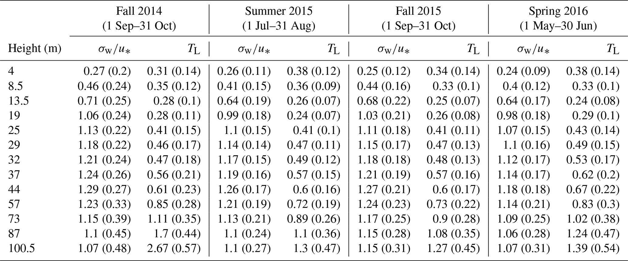
The level of coupling between the Norunda forest canopy and the atmospheric boundary layer was also investigated using the decoupling factor Ω as described in Goldberg and Bernhofer (2001). The decoupling factor Ω is given by

$$\begin{array}{}\text{(A2)}& \mathrm{\Omega }={\displaystyle \frac{s+\mathit{\gamma }}{s+\mathit{\gamma }\left(\mathrm{1}+\frac{r_{\text{s}}}{r_{\text{a}}},\right)}},\end{array}$$

where s is the slope of the saturation vapor pressure curve (Pa K⁻¹), γ is the psychrometric constant (Pa K⁻¹), r_a is the aerodynamic resistance, and r_s is the canopy resistance.

The decoupling factor Ω can range from 0 to 1. It quantifies the link between conditions at the canopy surface to the above-canopy atmosphere. Ω values near to 0 indicate aerodynamically well-coupled conditions. This is characterized by strong transpiration control by stomatal resistance and the vapor pressure deficit between the canopy surface and the atmosphere. Ω values near to 1 indicate aerodynamically decoupled conditions. In this case, transpiration is largely controlled by the available energy (Jarvis and McNaughton, 1986).

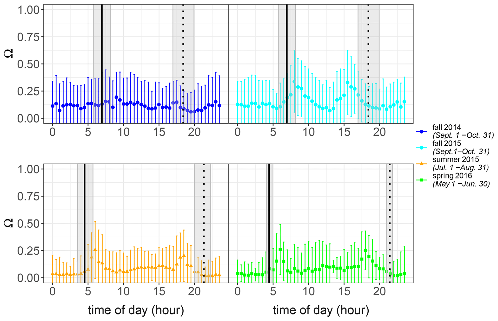
Figure A1 Diurnal behavior of the decoupling factor Ω for the seasonal periods presented in Fig. 6. Points show the 30 min average, and error bars indicate the standard deviation.

In Goldberg and Bernhofer (2001), the resistances r_a and r_s are estimated based on the assumption that the heat transport only depends on aerodynamic resistance and that the moisture transport only depends on canopy and aerodynamic resistance. Based on this, Goldberg and Bernhofer (2001) estimate that

$$\begin{array}{}\text{(A3)}& r_{\text{a}}=\mathit{\rho }{c}_{\text{p}}\left(T_{\mathrm{0}}-T\right)/H\end{array}$$

and

$$\begin{array}{}\text{(A4)}& r_{\text{s}}=\mathit{\rho }L\left(q_{\text{s}}\left(T_{\mathrm{0}}\right)-q\right)/LE-r_{\text{a}},\end{array}$$

where ρ is the air density (kg m⁻³), and c_p and L are the specific heat capacity of dry air (J K⁻¹ kg⁻¹) and latent heat of vaporization (J kg⁻¹). The values T₀ and q_s (T₀) are the temperature (^∘C) and the specific saturation humidity (g kg⁻¹), respectively, of the active canopy surface (in this case, for this 2014–2016 campaign period, the canopy height was at 28 m height for the Norunda forest). Meanwhile, T and q are the temperature (^∘C) and the specific humidity (g kg⁻¹), respectively, of the chosen atmospheric reference layer above the forest canopy (in this case, it was chosen to be at 57 m on the Norunda flux tower). The values H and LE represent the sensible heat flux (W m⁻²) and latent heat flux (W m⁻²), respectively, between the canopy surface and the chosen reference layer above the canopy.

For the campaign, Ω typically varied between 0.1 and 0.6. The nighttime–daytime transition did appear to have an influence on the coupling, with peaks in the decoupling factor occurring at sunrise and sunset times. Regarding seasonal dependence, there tended to be more decoupling during the spring and fall seasons than in the summer. An example of the estimated decoupling factors for several seasons is shown below.