the Creative Commons Attribution 4.0 License.
the Creative Commons Attribution 4.0 License.
 | 04 Jul 2023
Microwave radiometer observations of the ozone diurnal cycle and its short-term variability over Switzerland
Klemens Hocke
Eliane Maillard Barras
Shengyi Hou
Quentin Errera
Alexander Haefele
Axel Murk
In Switzerland, two ground-based ozone microwave radiometers are operated in the vicinity of each other (ca. 40 km): the GROund-based Millimeter-wave Ozone Spectrometer (GROMOS) in Bern (Institute of Applied Physics) and the Stratospheric Ozone MOnitoring RAdiometer (SOMORA) in Payerne (MeteoSwiss). Recently, their calibration and retrieval algorithms have been fully harmonized, and updated time series are now available since 2009. Using these harmonized ozone time series, we investigate and cross-validate the strato–mesospheric ozone diurnal cycle derived from the two instruments and compare it with various model-based datasets: the dedicated GEOS-GMI Diurnal Ozone Climatology (GDOC) based on the Goddard Earth Observing System (GEOS-5) general circulation model, the Belgian Assimilation System for Chemical ObsErvations (BASCOE) – a chemical transport model driven by ERA5 dynamics, and a set of free-running simulations from the Whole Atmosphere Community Climate Model (WACCM). Overall, the two instruments show very similar ozone diurnal cycles at all seasons and pressure levels, and the models compare well with each other. There is a good agreement between the models and the measurements at most seasons and pressure levels, and the largest discrepancies can be explained by the limited vertical resolution of the microwave radiometers. However, as in a similar study over Mauna Loa, some discrepancies remain near the stratopause, at the transition region between ozone daytime accumulation and depletion. We report similar delays in the onset of the modelled ozone diurnal depletion in the lower mesosphere.
Using the newly harmonized time series of GROMOS and SOMORA radiometers, we present the first observations of short-term (sub-monthly) ozone diurnal cycle variability at mid-latitudes. The short-term variability is observed in the upper stratosphere during wintertime, when the mean monthly cycle has a small amplitude and when the dynamics are more important. This is shown in the form of strong enhancements of the diurnal cycle, reaching up to 4–5 times the amplitude of the mean monthly cycle. We show that BASCOE is able to capture some of these events, and we present a case study of one such event following the minor sudden stratospheric warming of January 2015. Our analysis of this event supports the conclusions of a previous modelling study, attributing regional variability of the ozone diurnal cycle to regional anomalies in nitrogen oxide (NOx) concentrations. However, we also find periods with an enhanced diurnal cycle that do not show much change in NOx and where other processes might be dominant (e.g. atmospheric tides). Given its importance, we believe that the short-term variability of the ozone diurnal cycle should be further investigated over the globe, for instance using the BASCOE model.
- Article
(13279 KB) - Full-text XML
-
Supplement
(1789 KB) - BibTeX
- EndNote


Beyond its role in the protection of earth from harmful ultraviolet radiation, ozone is a key species in the energy balance of the middle atmosphere, strongly influencing the radiation budget and thermal state of the stratosphere and mesosphere. Following the success of the Montreal Protocol in 1987, full recovery of the ozone layer is expected for the 21st century with significant regional variability and uncertainties. In particular, there is a high degree of uncertainty about the lower stratospheric ozone recovery, and there is increasing observational evidence that ozone is still declining at some locations in the lower stratosphere (Ball et al., 2018; Maillard Barras et al., 2022a; Godin-Beekmann et al., 2022), without satisfactory explanation to date.
Ozone is a very reactive molecule involved in many (photo-)chemical reactions in the middle atmosphere. The set of pure oxygen photochemical reactions leading to the production and destruction of ozone was first described by Chapman (1930) and is known as the Chapman cycle. Together with catalytic depletion cycles involving many different species (NOy, Cly, HOy, etc.), they mostly drive the ozone amount in the middle atmosphere at multiple timescales. In particular, ozone concentrations are subject to complex diurnal cycle patterns depending on the geographic location, altitude, season, and other factors (Schanz et al., 2014), which makes it both important and difficult to fully take into account in models or observations.
The importance of the ozone diurnal cycle in the mesosphere has been recognized early through the use of photochemical models and from early measurements (e.g. Prather, 1981; Vaughan, 1982; Pallister and Tuck, 1983; Zommerfelds et al., 1989). Its main patterns are well known and have been successfully observed and modelled (Connor et al., 1994; Ricaud et al., 1991; Huang et al., 1997). In the stratosphere though, the ozone diurnal cycle is much weaker which makes accurate observations challenging. However, it needs to be taken into account when comparing different observing systems or to compute accurate trends (Bhartia et al., 2013; Maillard Barras et al., 2020). In recent years, there has been a renewed interest to improve the consideration of the diurnal variations of ozone and nitrogen oxides in satellite measurements (Frith et al., 2020; Schanz et al., 2021; Strode et al., 2022), partly because of the remaining uncertainties in post-2000 stratospheric ozone trends. For instance, Frith et al. (2020) used a modified version of the GEOS-5 model to produce a global, zonally averaged ozone diurnal climatology: the GEOS-GMI Diurnal Ozone Climatology (GDOC). The idea was to publish an easy-to-use climatology of scaling factors to account for ozone diurnal variability in intercomparison studies or for the creation of a merged ozone dataset. More recently, Strode et al. (2022) developed similar year-specific scaling factors for comparisons with the SAGE III/ISS measurements.
To validate such diurnal scaling factors, accurate observations are needed at different altitudes and locations. However, such observations remain relatively sparse and challenging, especially in the stratosphere where the ozone diurnal cycle amplitude is small. Also, many satellites are sun synchronous or use the sun as source, which limits their ability to derive full diurnal cycles. Some satellite-based ozone diurnal cycles have been successfully derived, however, from SAGE/ISS (Sakazaki et al., 2013, 2015) and from SABER on the Thermosphere Ionosphere Mesosphere Energetics and Dynamics (TIMED) satellite (Huang et al., 2010a). Although the satellite-based observations offer a global view on the ozone diurnal cycle, they do need to aggregate data in space or time to derive a diurnal cycle, therefore blurring any short-term or regional fluctuations in the cycle amplitude.
Passive microwave ground-based radiometers (MWRs) are well suited for ozone diurnal cycle observations, because they operate continuously and do not use the sun as a source. These instruments have been used successfully by different groups to monitor the diurnal cycle, not only in the mesosphere but also in the stratosphere (Connor et al., 1994; Schneider et al., 2005; Haefele et al., 2008; Parrish et al., 2014; Studer et al., 2014; Schranz et al., 2018). In the tropics, Parrish et al. (2014) derived detailed stratospheric ozone diurnal cycles over Mauna Loa from MWR measurements and compared them with satellite measurements and the Goddard Earth Observing System Chemistry Climate Model (GEOSCCM). They found a good agreement between the MWR and satellite observations as well as remaining discrepancies with the model in the upper stratosphere (3.2 to 1.8 hPa). In the polar region, Schranz et al. (2018) found larger discrepancies between MWR measurements and SD-WACCM simulations over Ny-Ålesund but only focused on a single year of measurements.
In this contribution, we derive updated ozone diurnal cycles over Switzerland from two co-located (ca. 40 km) ground-based MWRs between 2010 and 2022. The time series have recently been fully reprocessed with a harmonized algorithm (Sauvageat et al., 2022b), and they provide a unique set of measurements to study the ozone diurnal cycle and validate model simulations over the mid-latitudes. Compared to the three previous studies on ozone diurnal cycle over Switzerland (Zommerfelds et al., 1989; Haefele et al., 2008; Studer et al., 2014), this study combines the two MWRs over an extended time period (>10 years) and focuses on the time where the two instruments used the same digital spectrometer (after 2009). The combination of the spectrometer update and of the recent harmonization extended the altitude range and improved the sensitivity of the ozone retrievals. We obtain significant improvements in the updated stratospheric ozone diurnal cycle measured by the GROund-based Millimeter-wave Ozone Spectrometer (GROMOS) in Bern. In fact, the study from Studer et al. (2014) showed overestimated diurnal cycle amplitude compared to the model simulations. Although it was focused on the time period when GROMOS used a filter bank spectrometer (before 2009), we believe that part of the discrepancies were also due to the retrieval algorithm. Given that this instrument provided one of the main references for ozone diurnal cycle comparison studies over the mid-latitudes in the last decade, we believe that it is highly valuable to present in detail these updated results.
In fact, the objective of the present study is multiple. First we use the harmonized time series to derive the updated diurnal cycle above Switzerland and provide a comparative basis for different models at mid-latitudes. We especially aim at providing an additional validation for the dedicated GEOS-GMI Diurnal Ozone Climatology (GDOC), which has been published for use as a data analysis tool. In addition, we compare our measurements with two other types of model-based datasets: the Belgian Assimilation System for Chemical ObsErvations from Envisat (BASCOE) chemistry transport model (CTM) and the Whole Atmosphere Community Climate Model (WACCM) chemistry climate model (CCM). Finally, we present the first observations of short-term (sub-monthly) ozone diurnal variability and investigate the causes for such variations. We use the global, high-resolution simulations of BASCOE coupled with reanalysis data from ERA5 (Hersbach et al., 2020) to cross-validate our observations. We discuss a case study of the winter 2014–2015 and provide other examples where short-term fluctuations of the ozone diurnal cycle were observed.
The publication is organized as follows: Sect. 2 introduces the datasets and the methods used to compute the ozone diurnal cycle. Section 3 presents the results including the monthly ozone profile comparisons (Sect. 3.1), the intercomparisons of the monthly averaged ozone diurnal cycle over Bern (Sect. 3.2), and an example of observed short-term variability during the boreal winter 2014–2015 (Sect. 3.3). Finally, Sect. 4 presents a summary of the main results and some conclusions.
In the following, we present succinctly the datasets and the methods used in our study. Regarding the datasets, we focus mostly on the microwave radiometer time series and on the main model characteristics, and we provide references for the reader for additional details. Also, we summarize the most important features and relevant publications for each dataset in Table 1.
2.1 Microwave ground-based radiometers
Microwave ground-based radiometers (MWRs) are passive remote sensing instruments that can be used to derive trace gas or temperature profiles in the atmosphere. MWRs measure the emission of atmospheric molecules in the microwave frequency range. Therefore, they do not rely on the sun for their observations and provide quite high temporal resolution and continuous sampling, which makes them an excellent candidate for diurnal cycle studies.
In Switzerland, two ozone microwave radiometers are operated close to each other (ca. 40 km) on the Swiss Plateau. The GROund-based Millimeter-wave Ozone Spectrometer (GROMOS) is operated by the Institute of Applied Physics (IAP) at the University of Bern (46.95∘ N, 7.44∘ E; 560 ) since 1994 and the Stratospheric Ozone MOnitoring RAdiometer (SOMORA) is operated by the Federal Office of Meteorology and Climatology MeteoSwiss in Payerne (46.82∘ N, 6.94∘ E; 491 ) since 2000. The two instruments have been designed at the IAP, have similar design, and use the rotational ozone emission line at 142.175 GHz to derive strato–mesospheric ozone profiles. Also, they have similar viewing geometries; both observe the sky at ∼40∘ elevation angle and experience similar atmospheric opacity conditions. Following discrepancies identified between the two instruments (Bernet et al., 2019; SPARC/IO3C/GAW, 2019), a complete harmonization of the data processing has recently been performed for GROMOS and SOMORA. It resulted in harmonized, continuous, hourly time series of strato–mesospheric ozone starting in 2009, which are now freely available (Sauvageat et al., 2022b).
The vertical resolution of the MWRs is quite coarse (∼10 km up to 3 hPa and ∼15 km above), and the vertical extent of the ozone profile is from 60 to 0.02 hPa (∼20 to 75 km), corresponding to the range where the a priori contribution to the retrieved profile is lower than 20 % (Fig. 1). The MWRs coarser vertical resolution needs to be taken into account for intercomparison with higher-resolution datasets (e.g. models), also for the diurnal cycle comparisons. The usual way is to apply a smoothing procedure to the higher-resolution dataset for the comparisons. In our study, we use the classical “averaging kernel smoothing” which essentially convolves the high-resolution dataset with the averaging kernels (AVKs) of the MWR retrieval using Eq. (1) (Rodgers and Connor, 2003). Equation (1) also applies the effect of the a priori contribution of the MWR retrievals onto the higher-resolved profile and is usually expressed as
with xa being the a priori profile (derived from monthly WACCM profiles in our case), A the averaging kernel matrix, and x and xc respectively the original and convolved high-resolution profiles.
GROMOS and SOMORA essentially have the same sensitivity, allowing us to compare their observations directly. It can be seen by looking at the mean AVKs and the measurement contribution of the retrievals shown in Fig. 1. This also means that there is only little difference whether we use GROMOS or SOMORA AVKs for the smoothing procedure. In the following, all convolutions on the higher-resolution profiles are performed using the GROMOS AVKs. Figure 1 shows the mean AVKs of the full GROMOS and SOMORA time series; however, for all the convolutions we use the appropriate monthly daytime or nighttime AVKs.
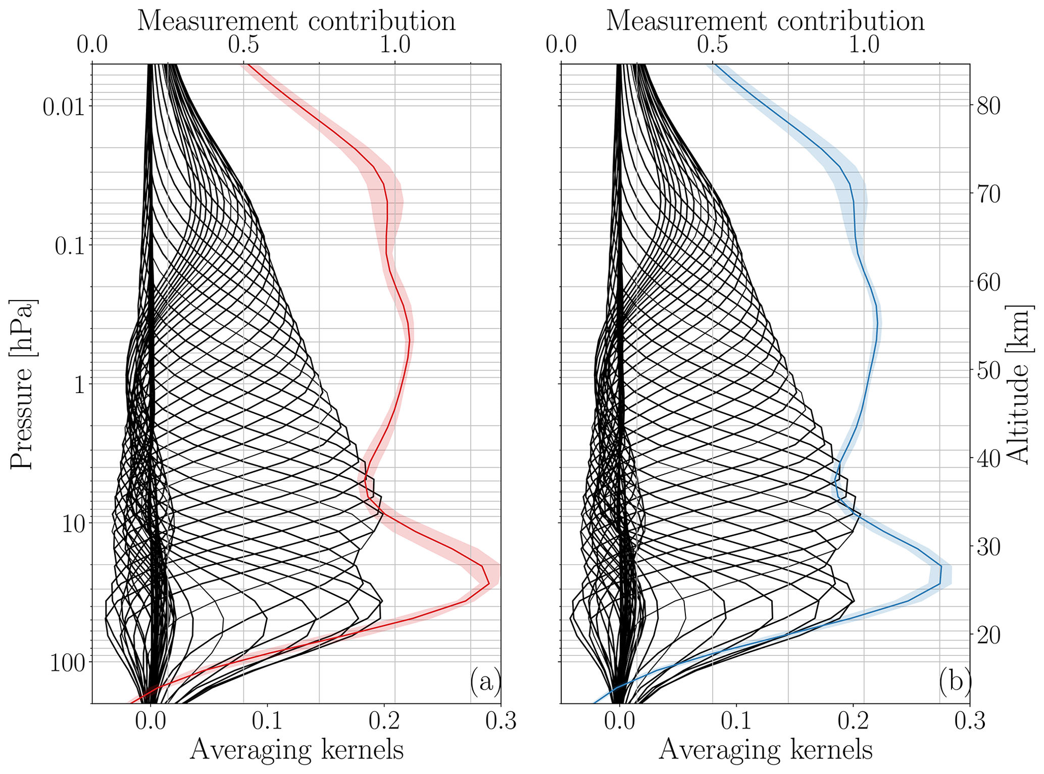
Figure 1Mean averaging kernels and measurement contribution for (a) GROMOS and (b) SOMORA. The black lines are the averaging kernel at individual pressure levels, whereas the colour lines are the respective measurement contribution (see upper x axis). The shaded colour area shows the standard deviation of the measurement contribution.
2.1.1 Satellite measurements
For validation purposes, we use measurements from the Microwave Limb Sounder (MLS) mounted on the Aura spacecraft (Waters et al., 2006). Since its launch in July 2004, the MLS instrument has been used extensively for trace gas observations and is one of the main measurement references for global ozone monitoring studies. More specifically, we use the latest ozone retrieval product (v5), following the screening guidelines provided in Livesey et al. (2022). The MLS ozone vertical resolution ranges from ∼2.5 to ∼5 km in the stratosphere and mesosphere, whereas its horizontal resolution ranges between 300 and 500 km. As spatial co-location criteria, we keep only measurements around Switzerland (±1.8∘ in latitude and ±5∘ longitude). Aura overpasses Switzerland twice a day, at 02:20 and 13:10 LST (local solar time), thus providing the day-to-night ozone ratios but not the full diurnal cycle. In Sect. 3.3, we also show some measurements of temperature and nitrous oxide from MLS; however, as higher temporal resolution was needed for the short-term analysis, these were obtained with more relaxed co-location criteria (±3.6∘ latitude and ±10∘ longitude) but following the same screening guidelines (Livesey et al., 2022).
2.2 Model-based datasets
2.2.1 GDOC
GEOS-GMI Diurnal Ozone Climatology (GDOC) is a model-based climatology of ozone diurnal cycle derived from the NASA Goddard Earth Observing System general circulation model, version 5 (GEOS-5). The goal of this climatology is to provide a simple data analysis tool to account for ozone diurnal variability, e.g. when comparing different satellite profiles.
For the production, GEOS-5 was run in replay mode constrained to 3-hourly MERRA-2 assimilated meteorological fields from January 2017 to December 2018 (see Orbe et al., 2017; Frith et al., 2020, and references therein for model details). As final product, the GDOC provides zonally averaged (on 5∘ latitude bands) ozone diurnal cycles from 90 to 0.3 hPa (∼20 to 55 km) with equivalent vertical resolution of ∼1 km and a time resolution of 30 min. The climatology is also available (on request) on original model levels but has not been evaluated below 30 hPa and above 0.3 hPa, which is the reason why we chose not to use it outside of this pressure range.
It provides monthly climatological ozone values as a function of local solar time (LST) normalized to midnight ozone values. The GDOC does not contain the original ozone profiles, which prevents the application of the averaging kernel smoothing procedure on this dataset. Consequently, we only show the original high-resolution profile from the GDOC dataset.
2.2.2 BASCOE
This study uses the chemistry transport model (CTM) simulation performed by the Belgian Assimilation System for Chemical ObsErvations (BASCOE; Errera and Fonteyn, 2001; Errera et al., 2008). The simulation covers the 2010–2020 period and is driven by 6-hourly wind and temperature fields taken from ERA5 (Hersbach et al., 2020), preprocessed in a similar set-up as described in Chabrillat et al. (2018) and Minganti et al. (2022). The simulation is performed with a time resolution of 30 min, a horizontal resolution of 2∘ in latitude and 2.5∘ in longitude, and 42 hybrid pressure levels from the surface to 0.01 hPa with a vertical resolution between 1 km in the lower stratosphere and 4 km in the lower mesosphere. The BASCOE model focuses on the calculation of the chemical composition of the stratosphere. It includes around 60 chemical species interacting through around 200 reactions (gas phase, photolysis, and heterogeneous) and a parametrization to account for the effect of sulfate aerosols and polar stratospheric clouds on the stratospheric composition (Huijnen et al., 2016). Background sulfate aerosols are taken from the Climate Model Intercomparison Project Phase 6 (CMIP6) recommendations, whereas surface emissions of long-lived species are taken from the “Historical Greenhouse Gas Concentrations” (HGGC) recommendations also produced for CMIP6 experiments (Meinshausen et al., 2017). The model provides a realistic composition of the stratosphere when compared to independent observations (see, for example, Prignon et al., 2021; Minganti et al., 2020, 2022). For this study, the model outputs have been interpolated at the location of Bern so that they can be compared with the two MWRs.
2.2.3 WACCM
We also use results from the Whole Atmosphere Community Climate Model (WACCM), version 4, in the configuration described by Schanz et al. (2021). WACCM is a fully coupled global chemistry climate model developed at the National Center for Atmospheric Research (NCAR) with a stratospheric chemistry module based on the Model of Ozone and Related Chemical Tracers (MOZART) (Kinnison et al., 2007). It simulates the atmosphere from the surface to ∼150 km altitude, with a vertical resolution between 1.1 and 2 km in the middle atmosphere. WACCM was run with a horizontal resolution of 4∘ latitude by 5∘ longitude, and for our study we use the closest grid point to both Bern and Payerne, which corresponds to 46∘ N and 5∘ E. The model was run with the pre-defined free-running “F 2000” scenario, simulating a perpetual year 2000 but without data nudging.
Sauvageat et al. (2022b)Sauvageat et al. (2022b)Waters et al. (2006); Froidevaux et al. (2008)Frith et al. (2020)Errera et al. (2008)Garcia et al. (2007); Marsh et al. (2013)Hersbach et al. (2020)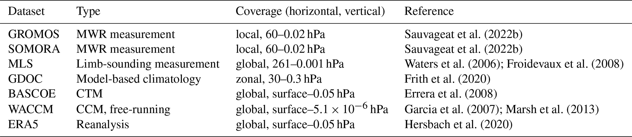
2.3 Ozone profiles and day-to-night ratios
Before computing the ozone diurnal cycle from our different datasets, we first compare their monthly averaged ozone profiles during daytime and nighttime and compute their day-to-night ratios. We compare our two MWRs with MLS and BASCOE, all averaged over the time period 2010–2020, therefore removing most of the year-to-year variability. WACCM is not included in these comparisons for two reasons. First, we use the free-running WACCM simulations for a single year, and it would make no sense to compare it with the other datasets which are multi-year averages, especially in the wintertime when dynamics are an important modulator of the ozone amount. Second, the monthly averaged WACCM ozone profiles are actually used as a priori data for our MWR retrievals; therefore, they can not be used for validation against the retrieved MWR profiles.
For the ozone profile comparisons, we choose to use profiles whose time corresponds approximately to the MLS overpass times (02:20 and 13:10 LST). Therefore, we keep timestamps between 12:00 and 15:00 LST for the daytime profiles and between 01:00 and 04:00 LST for the nighttime profiles, regardless of the dataset. As explained in Sect. 2.1, we convolve the BASCOE simulations and the MLS measurements with monthly averaged daytime or nighttime GROMOS AVKs.
2.4 Ozone diurnal cycle
Similarly to the GDOC climatology, we choose to express the ozone diurnal cycle as ratio of ozone volume mixing ratios (VMRs) relative to the midnight value. To compute the reference midnight value (O3,NT in Eq. 1), we have used different time periods to reflect the different time resolutions of the datasets. For the MWRs (∼1 h time resolution), we compute the midnight reference value by taking an average of two nighttime measurements between 23:00 and 01:00 LST. For WACCM and BASCOE (30 min time resolution), we use measurement between 00:00 and 01:00 LST, whereas the GDOC was normalized to the values between 23:45 to 00:15 LST (Frith et al., 2020).
For each hour and at each pressure level, we then compute the ratios to ozone at midnight using Eq. (2). To simplify the notation, we do not explicitly write the pressure dependence of all the terms.
To compare with the monthly GDOC climatology, we compute monthly averaged ΔO3(h) from GROMOS, SOMORA, WACCM, and BASCOE. For each dataset, we use the available time series, i.e. 12 years of data for the two MWRs (2010–2022), 10 years for BASCOE (2010–2020), and the 1 year of the WACCM free-running model run. For the MWRs, we additionally filtered the time series to remove the measurements done at very high tropospheric opacity (τ>1.5), as they result in lower quality retrievals and can potentially contaminate the monthly averages. To some extent, it also helps to limit any seasonal bias arising due to the summertime higher opacity, although it is difficult to rule out this effect completely (e.g. see discussion on the effect of the opacity on GROMOS and SOMORA in Sauvageat et al. (2022b)). For the diurnal cycle, the effect of this filtering is not very large, and for the interested reader the unfiltered version is provided in the Supplement (Figs. S5 to S16).
We compute errors on the MWRs and BASCOE ozone diurnal cycles as standard error of the mean (SEM). For each month and LST hour, we compute the standard deviation of ΔO3(h) and divide it by the square root of the number of ozone profiles available for each hour.
2.5 Short-term variability of the ozone diurnal cycle
In addition to monthly averaged ozone diurnal cycle, we also show observations of short-term (sub-monthly) variability of the ozone diurnal cycle. GROMOS and SOMORA provide a unique set-up for short-term ozone diurnal cycle observations, because they have continuous, hourly, co-located measurements. Therefore, we can use them to compute the ozone diurnal cycle on sub-monthly periods and cross-validate their measurements. Also, we use BASCOE simulations to compute the short-term variability of the ozone diurnal cycle over Switzerland and to investigate the cause of such variability.
In order to detect sub-monthly variations in the ozone diurnal cycle, we computed the day-to-night differences in ozone VMR for GROMOS, SOMORA, and BASCOE. More specifically, we compute the anomalies of the day-to-night differences () to a monthly climatology. As daily anomalies are too noisy, we average these differences on 5 d.
In this contribution, we focus on the winter 2014–2015 and use BASCOE and MLS data to investigate and discuss potential reasons explaining a specific event during this winter. For further studies, we provide along with this publication the full time series of daily anomalies for GROMOS, SOMORA, and BASCOE.
3.1 Monthly ozone profiles and day-to-night ratio
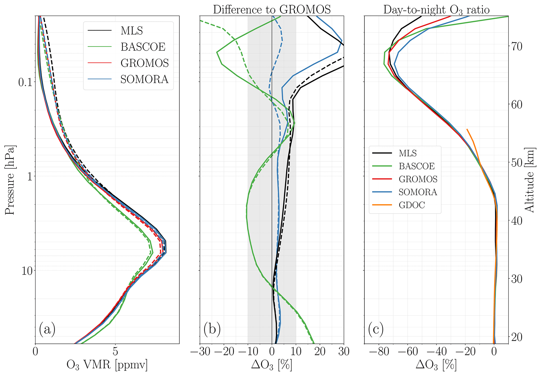
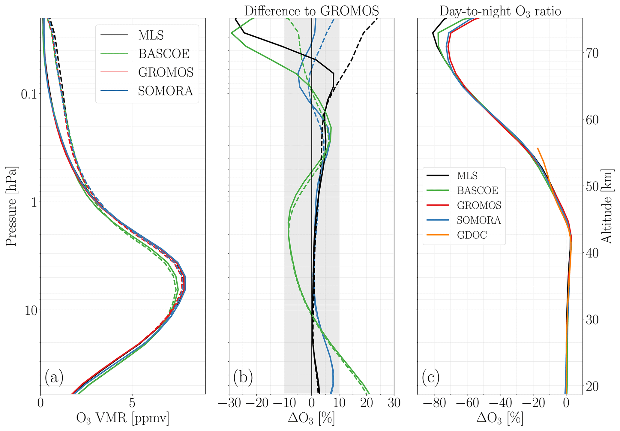
The comparisons of the monthly averaged ozone daytime and nighttime profiles and day-to-night ratios are shown in Fig. 2 for December and Fig. 3 for June as proxies for the winter and summer season. Figures A1 and A2 in Appendix A show similar comparisons for March and September, respectively. Similar comparisons but with respect to SOMORA MWR can be seen in the Supplement (Figs. S1 to S4). Overall we find a good agreement between measured ozone profiles (GROMOS, SOMORA, and MLS), with relative differences between the measured ozone profiles lower than 10 % up to 0.1 hPa. The differences between BASCOE and the MWR are within 15 % between 30 and 0.2 hPa, with slightly larger bias during the winter months. BASCOE notably underestimates ozone amounts in the upper stratosphere to lower mesosphere (up to ∼0.5 hPa) and overestimates ozone in the lower stratosphere, regardless of the month or the time of day. Above 0.2 hPa, the differences depend on the month considered, but the model tends to underestimate the daytime ozone profiles, leading to a small overestimation of the day-to-night depletion ratio over 0.2 hPa. The ozone deficit of BASCOE in the middle atmosphere is consistent with previous studies (Skachko et al., 2016) and could be due to an overestimation of NO2 in the model simulations, thereby enhancing catalytic ozone destruction though the so-called “Crutzen” cycle (Crutzen, 1970). Note that this deficit of middle-atmospheric ozone is found in other models as well (see, for example, Fig. 3.1 in SPARC, 2010).
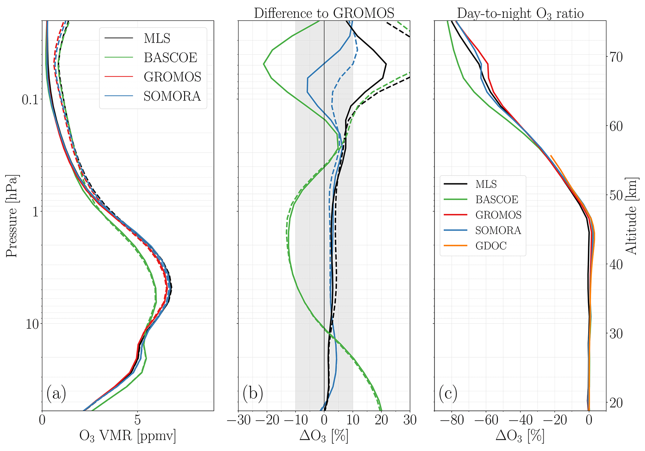
Figure 2(a) Monthly averaged profiles, (b) relative differences ((X-GRO)/GRO), and (c) day-to-night ratios of ozone VMR above Switzerland in December. In panels (a) and (b), the solid lines are the daytime profiles, whereas the dashed lines are the nighttime profiles.
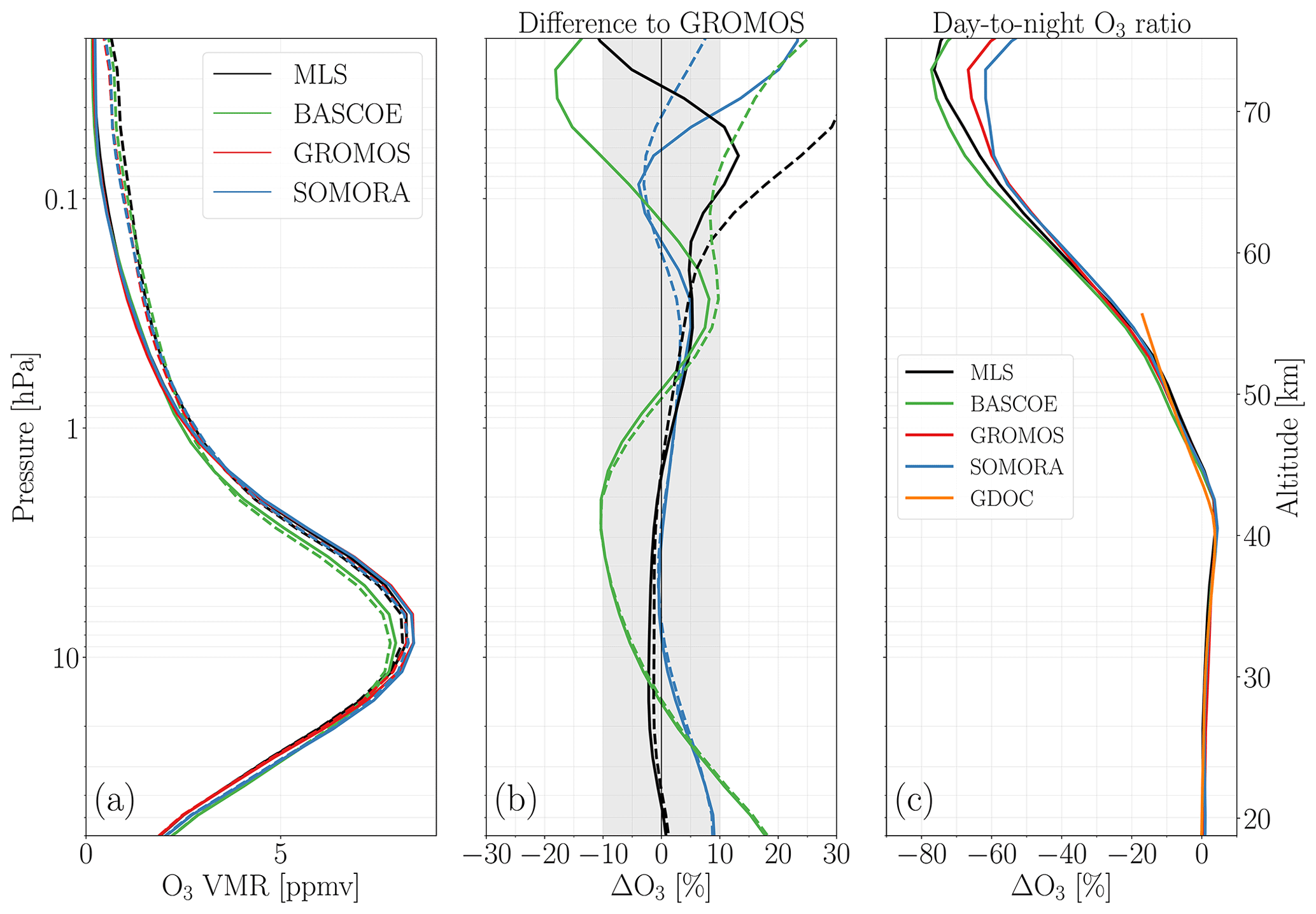
All datasets show the ozone daytime accumulation in the stratosphere and its transition to ozone daytime depletion around the stratopause (∼2–1 hPa). All datasets show stratospheric ozone accumulation during daytime (up to ∼1 hPa) with stronger amplitude during the summertime, and they all show the strong mesospheric ozone depletion during daytime, growing in amplitude with altitude. They agree quite well on the pressure at which peak accumulation and peak depletion occur. During summer, there is an excellent agreement between day-to-night ratios up ∼0.6 hPa. Above this pressure level, the GDOC climatology systematically underestimates the daytime ozone loss, leading to less negative day-to-night ratio than the other datasets. In the mesosphere, BASCOE and MLS compare well with the MWRs up to 0.05 hPa, with day-to-night ratios in agreement within 15 %.
3.2 Comparison of monthly ozone diurnal cycle
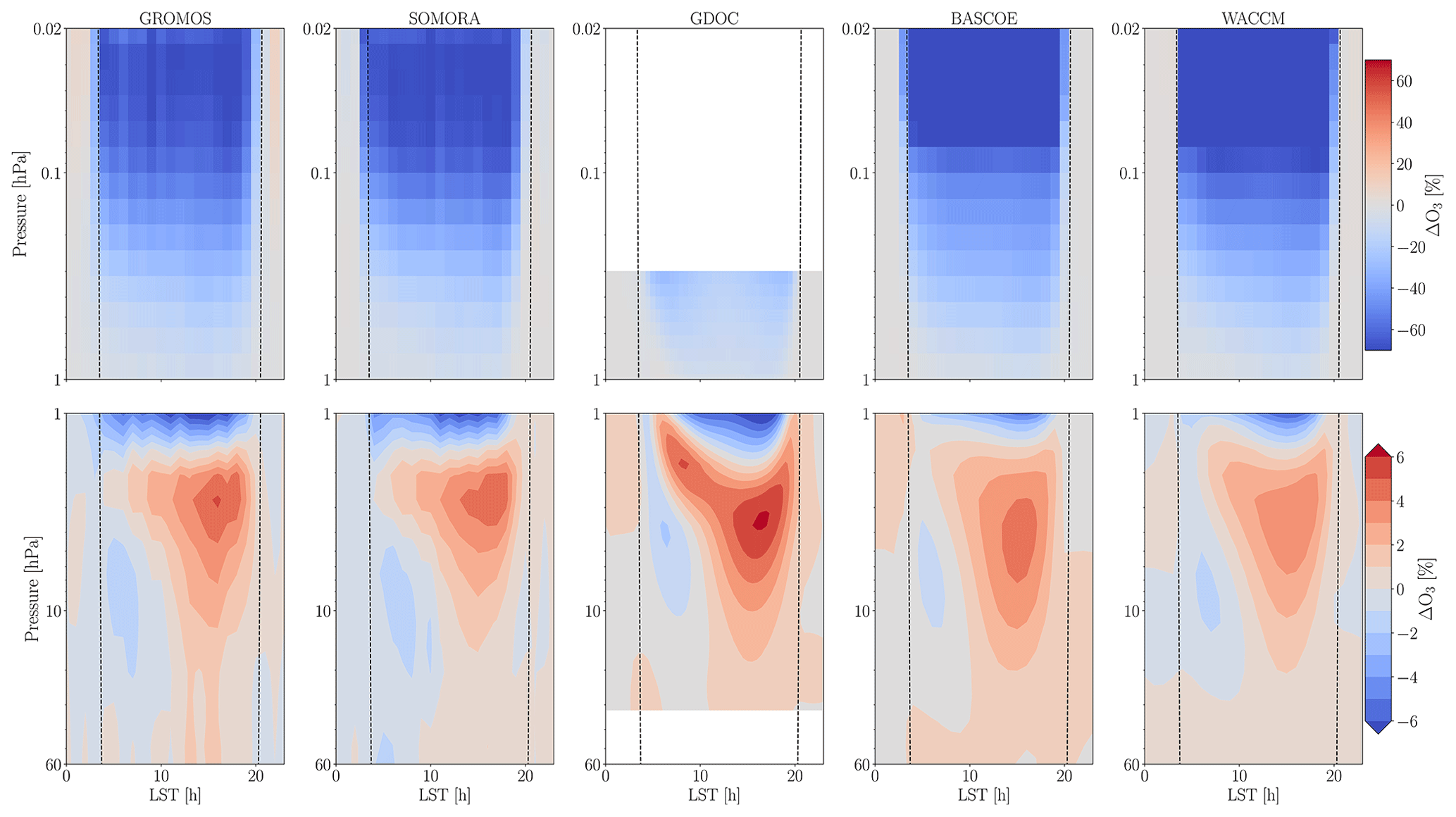
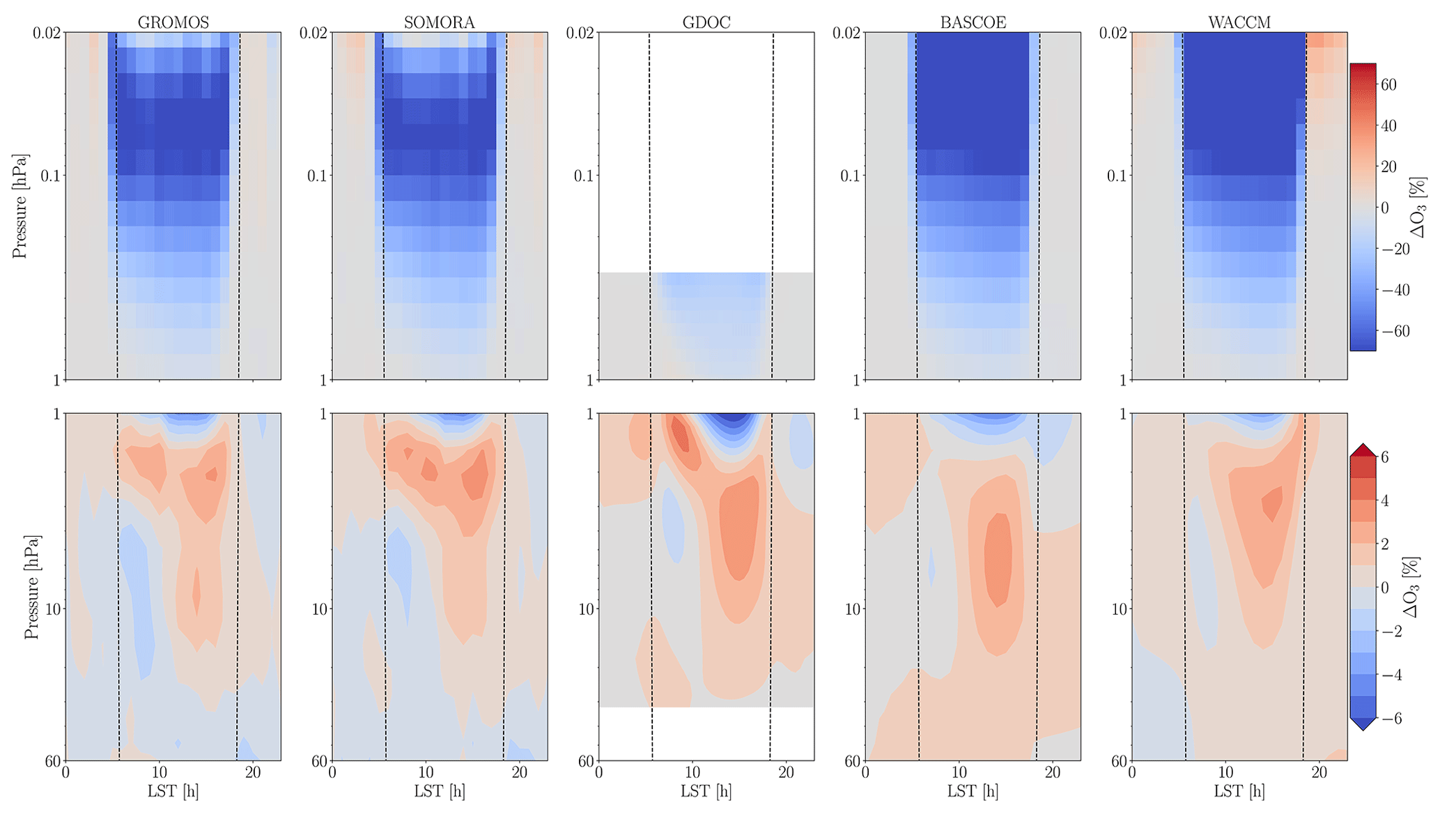
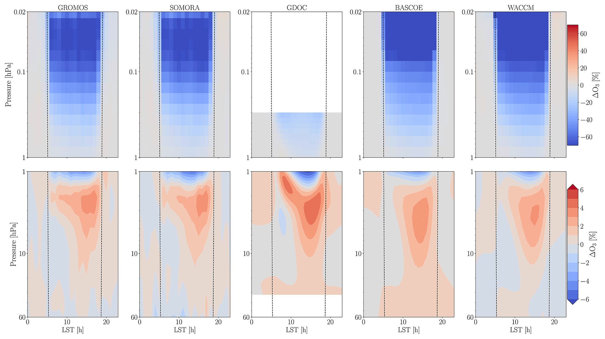
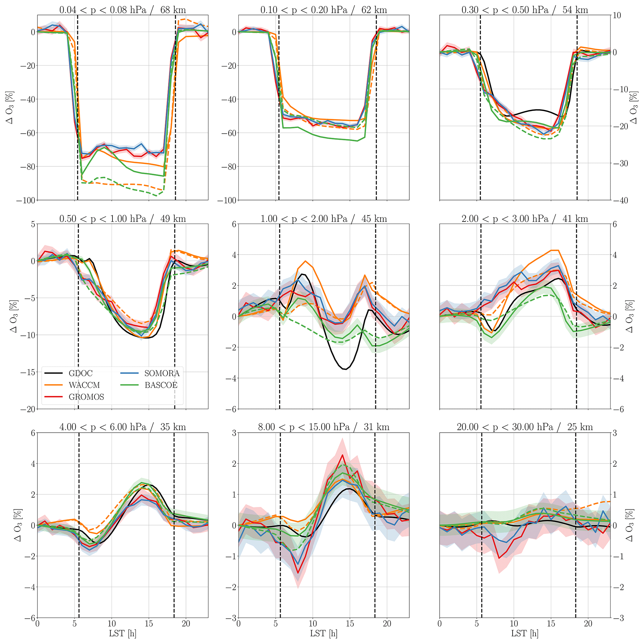
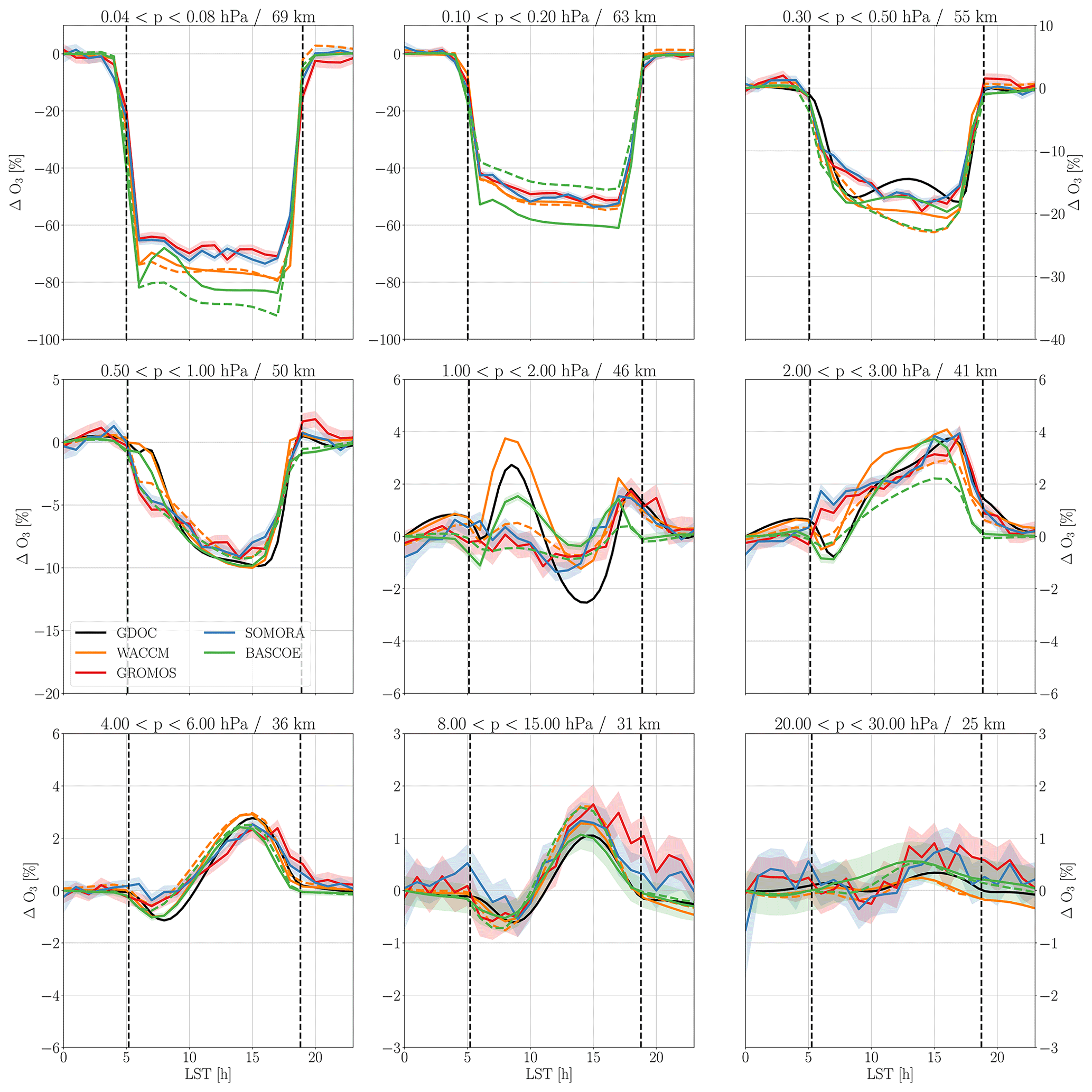
Going beyond the day-to-night ratio, full monthly diurnal cycles over Switzerland are shown for summer and winter in Figs. 4 and 5 for the two MWRs and the three model-based datasets (Figs. B1 and B2 in Appendix B show similar results for spring and autumn, respectively). These figures show the ratios to ozone midnight values as a function of the LST between 60 and 0.02 hPa (respectively 30 and 0.3 hPa for GDOC). As mentioned previously, the monthly averages correspond to different time periods for each dataset: 2010–2022 for GROMOS and SOMORA, 2010–2020 for BASCOE, 2017–2018 for the GDOC, and 2000 perpetual year for WACCM. Also, AVK smoothing procedures have been applied to the WACCM and BASCOE dataset but not to the GDOC. The original version without any AVK smoothing can be seen for all datasets in the Supplement. For better visualization, we also show these diurnal cycles averaged over nine selected pressure ranges. This is shown in Figs. 6 and 7 for winter and summer (in Figs. B3 and B4 in Appendix B for spring and autumn). These figures show the original cycle from each dataset together with the AVK smoothed cycle, which enables us to clearly see the effect of the AVK smoothing procedure on the high-resolution datasets. In order to better compare the different months and datasets, Fig. 8 shows vertical profiles of the diurnal cycle amplitude for all months and datasets. Here, the amplitude is defined as the percentage change between the maximum and the minimum normalized ozone ratios (ΔO3 as defined in Eq. 2) during the course of a day.
The new harmonized ozone time series from GROMOS and SOMORA have excellent agreement in ozone diurnal cycle. They agree well in patterns and amplitudes at all seasons and most altitudes. Some small discrepancies can be seen in summertime in the transition region (see, for example, July or August in Fig. 8); however, as shown in Sauvageat et al. (2022b), it is also the season where GROMOS and SOMORA experienced the larger discrepancies between their respective measurements. The two regimes of the ozone diurnal cycle are clearly visible in all datasets. Namely, the accumulation of ozone during daytime in the stratosphere and the depletion of ozone during daytime above ∼1 hPa are well captured by all datasets.
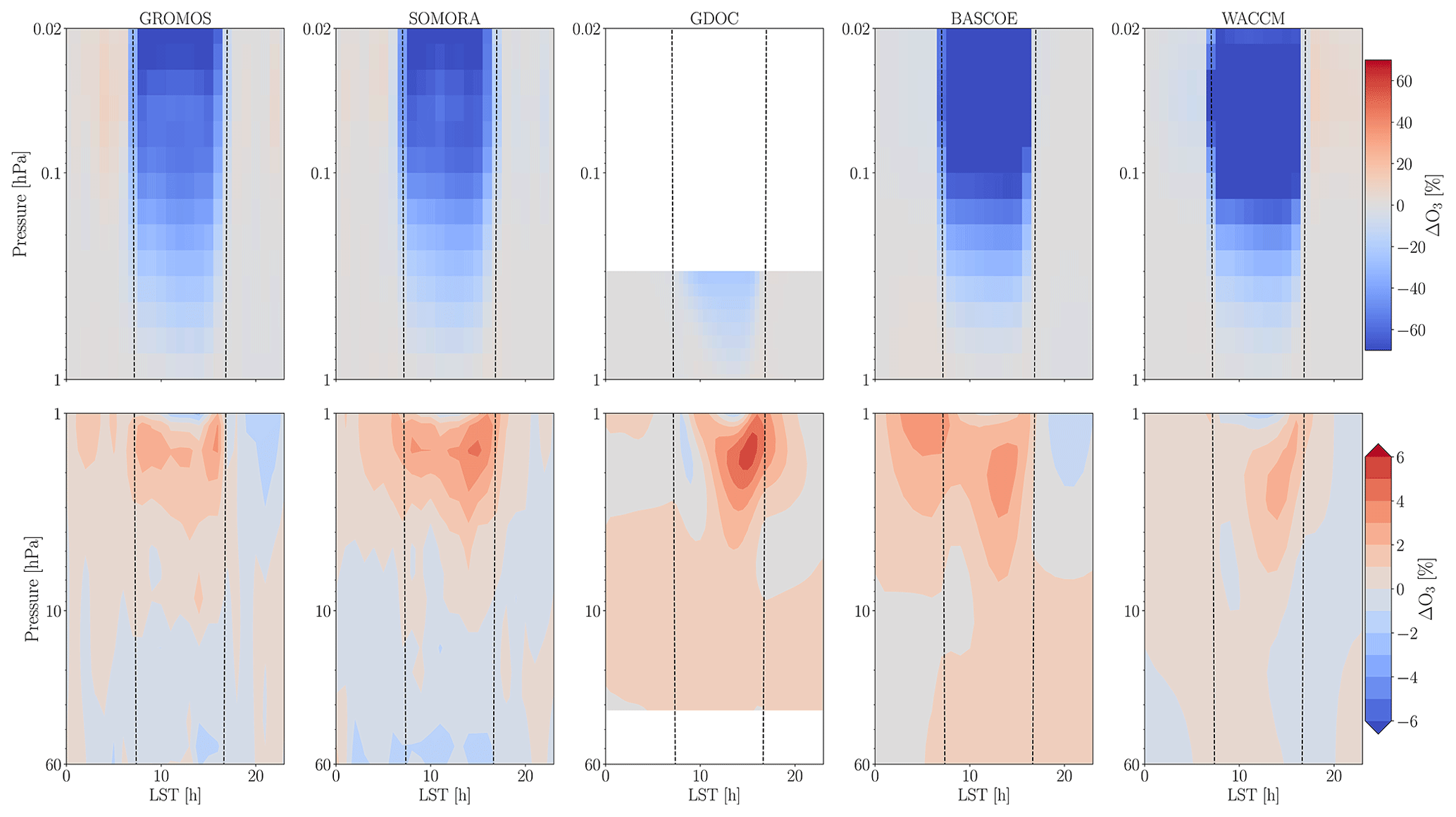
Figure 4Monthly averaged ozone diurnal cycle over Switzerland in December as seen in GROMOS, SOMORA, GDOC, BASCOE, and WACCM datasets. Note that only the BASCOE and WACCM datasets have been convolved with the AVKs of GROMOS as explained in Sect. 2.1.
Among the model datasets, we observe most discrepancies of the diurnal cycle amplitude by the GDOC during wintertime in the upper stratosphere (see January or February in Fig. 8). To some extent, these discrepancies could be due to the temporal (different averaging periods) and longitudinal (zonal mean in GDOC) variability, which are both smoothed out in the GDOC. As mentioned by Frith et al. (2020), this is also the season where the ozone diurnal cycle is smaller and where the model uncertainties are higher. Below, we will present a summary of the differences between the MWRs and the models, focusing on different altitude regions and discuss in more details the reasons for the observed discrepancies.
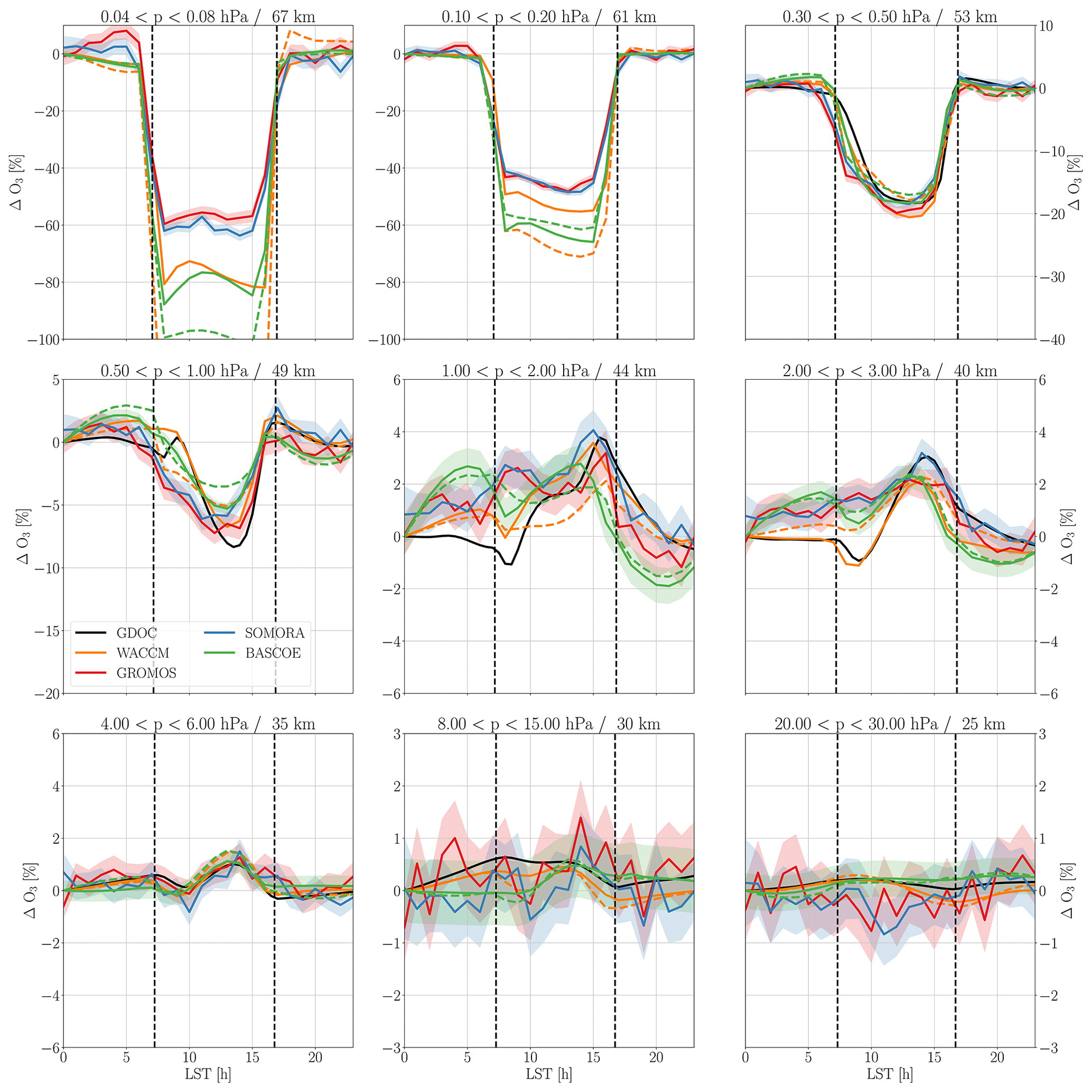
Figure 6Monthly averaged ozone diurnal cycle over Switzerland at four selected pressure ranges in December. For BASCOE and WACCM, we show both the diurnal cycle before (solid lines) and after convolution (dashed lines) of the dataset with the AVKs of GROMOS. To account for the large changes in the diurnal cycle amplitude with altitude, the scale of the y axis is adapted for each sub-plot.
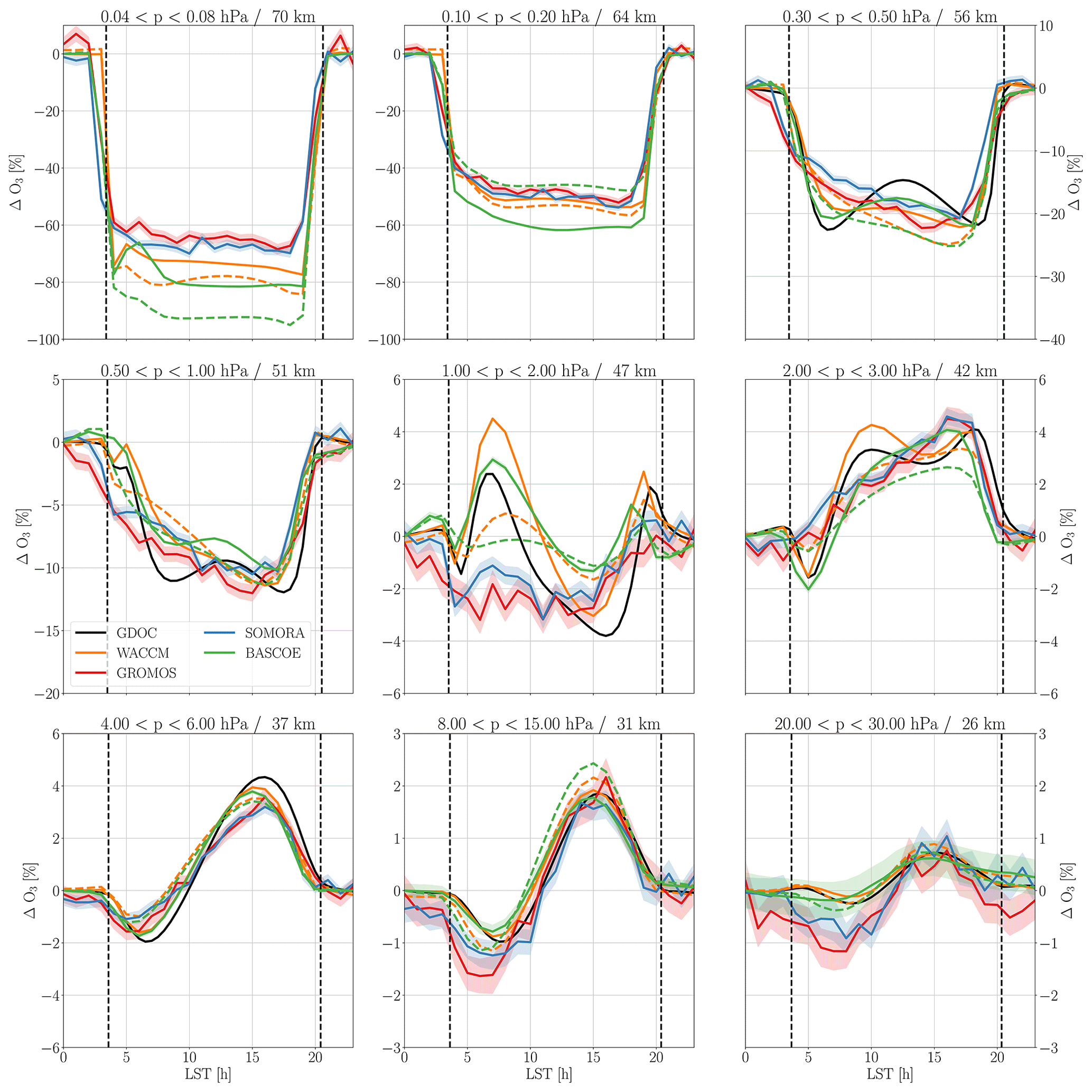
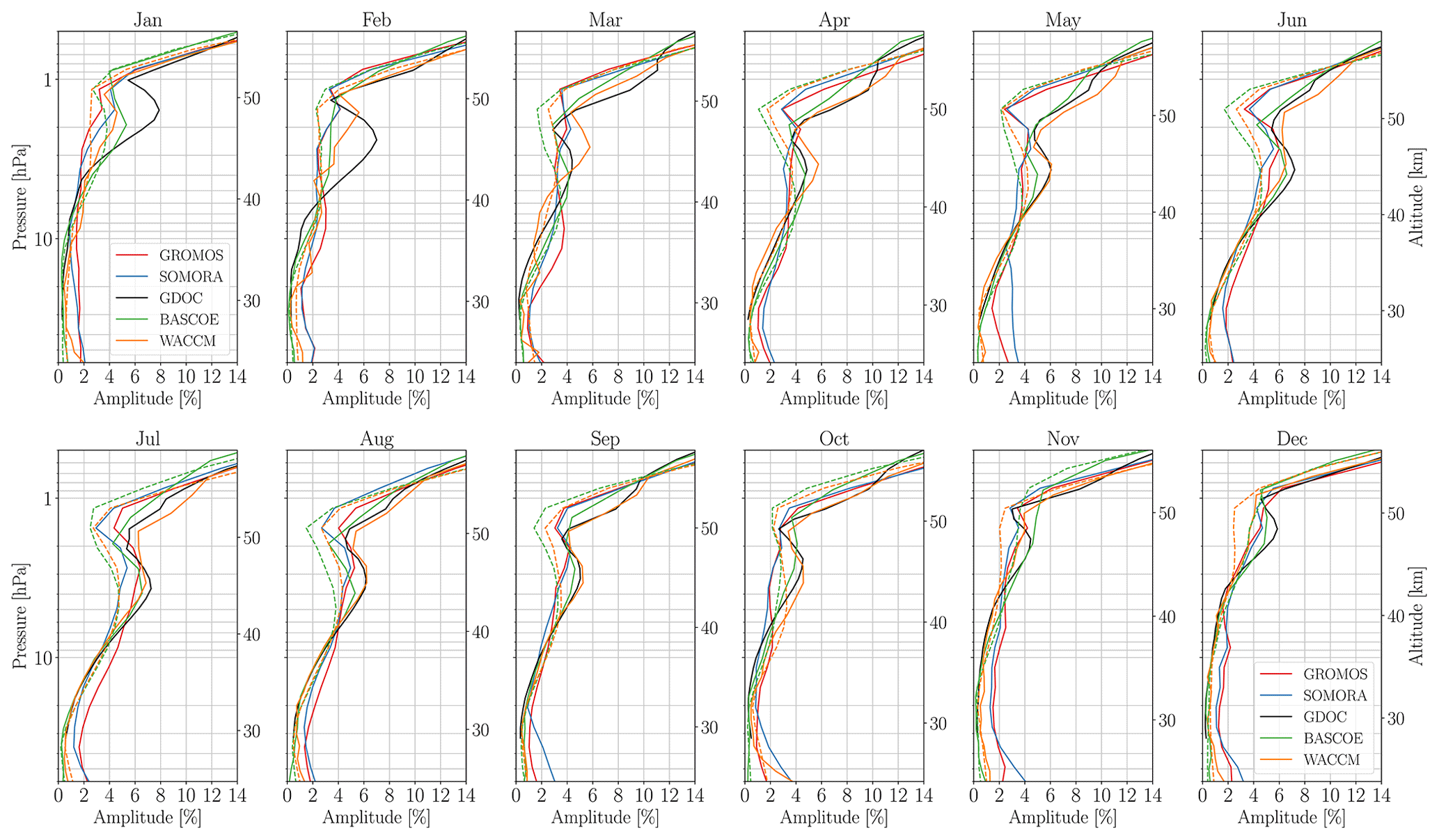
Figure 8Monthly averaged vertical profiles of the ozone diurnal cycle amplitude. It shows the percentage change between the maximum and the minimum ozone ratio values. The dashed lines show the model results after convolution with the AVKs of GROMOS.
3.2.1 Mesosphere (p<0.3 hPa)
Overall, we observe a tendency of the models to overestimate the diurnal ozone depletion in the mesosphere. It is mostly noticeable above ∼0.1 hPa where the sensitivity values of the MWRs are decreasing and where the measurement error is growing fast. Therefore, even if the effect of the lower sensitivity should be included through the AVK smoothing, biases above this altitude should be considered with care. Note that at this altitude, BASCOE also has a limited vertical resolution as it only uses two pressure levels above 0.1 hPa. Considering the above limitations, we still observe quite a good agreement of the upper mesospheric diurnal cycle at all seasons. In agreement with Parrish et al. (2014) but in contradiction with the conclusions from Studer et al. (2014), we do not observe a significant seasonal variation of the mesospheric diurnal cycle amplitude. This is in better agreement with the model results, which show similar amplitude throughout the year.
3.2.2 Lower mesosphere (1–0.3 hPa)
In the lower mesosphere, we note a consistent bias between the models and the observations around sunrise: the diurnal ozone depletion observed by the MWRs consistently starts earlier than the models. It is true for most months and could be partly explained by differences in the vertical resolution (e.g. see Fig. 7 at 51 and 56 km). Interestingly, it does not seem to impact the sunset period, which rules out potential errors arising from the time conversion between the different datasets. This feature was also observed by Parrish et al. (2014) over Mauna Loa, and it seems to persist even after application of the AVKs (not for all months though), which gives us confidence that it does not result from the a priori data.
3.2.3 Stratopause region (3–1 hPa)
Around the stratopause, we can clearly see the complex transition region between the mesospheric diurnal depletion and the stratospheric accumulation. This is where we notice the largest biases between our different datasets. In fact, we observe discrepancies among the three model-based datasets and between the observations and the models. The biases around the stratopause (1–3 hPa) are similar to the ones reported by Parrish et al. (2014) and Haefele et al. (2008), i.e. differing behaviour in the pre-dawn hours and after sunrise. They are seen at all seasons during daytime and reach values up to 2 % differences among the models themselves (e.g. between 1 and 2 hPa in Fig. 7). Between the models and the MWRs, the biases are significantly reduced by the application of the AVK smoothing procedure, but we still note biases up to 2 % in this region.
As will be shown in Sect. 3.3, the upper stratosphere and lower mesosphere are also experiencing short-term variability of the ozone diurnal cycle, which can influence the monthly averaged cycle. In particular, the datasets produced using only a few specific years (i.e. WACCM or GDOC in our case) will be influenced by the short-term variability of these years, whereas it will be smoothed out in the MWR or the BASCOE datasets which are averaged on 10 years or more. As shown in Fig. S11 from the Supplement of Frith et al. (2020), although the inter-annual variability is generally limited below 5 hPa and during summer, inter-annual variations up to 5 % around 0.5–1 hPa can be seen during wintertime in the mid-latitudes. This supports the existence of short-term variability in the ozone diurnal cycle and might therefore explain some of the remaining discrepancies near the stratopause region.
3.2.4 Middle and lower stratosphere (30–3 hPa)
In the middle and lower stratosphere, we observe the typical behaviour of the stratospheric ozone diurnal cycle: a small dip after sunrise followed by a gentle accumulation reaching a maximum in the late afternoon. The stratospheric cycle shows a high seasonal variability, with a maximum diurnal cycle amplitude around the summer solstice and lower diurnal variations during winter. In summer, we observe a peak amplitude of the ozone diurnal cycle of 3 %–4 % in the afternoon around 5 hPa in July, reducing to less than 2 % in the wintertime. For this reason, the dip after sunrise, attributed to rapid dissociation of NO2 at sunrise (Pallister and Tuck, 1983), is mostly visible during the summer months. Note that this is a significant improvement compared to the previous retrievals of the GROMOS time series, where the dip was not observed and where the amplitude of the stratospheric cycle was high compared to the models (Fig. 6a and b in Studer et al., 2014). With the new time series, the amplitude of stratospheric ozone cycle is well captured by GROMOS and SOMORA at most seasons. In fact, most of the discrepancies that we observe in the middle stratosphere are the consequences of the limited vertical resolution of the MWRs, whereas the differences of the lower stratosphere stay mostly within the error bars.
3.3 Short-term variability of the ozone diurnal cycle
In this section, we present the first measurements of short-term ozone diurnal cycle variability using the unique set-up offered by the co-located, hourly resolved measurements from GROMOS and SOMORA. To our knowledge, it is the first time that short-term variability of the ozone diurnal cycle is observed, and in the following we try to identify some of the reasons leading to such events, focusing on a case study from the boreal winter 2014–2015.
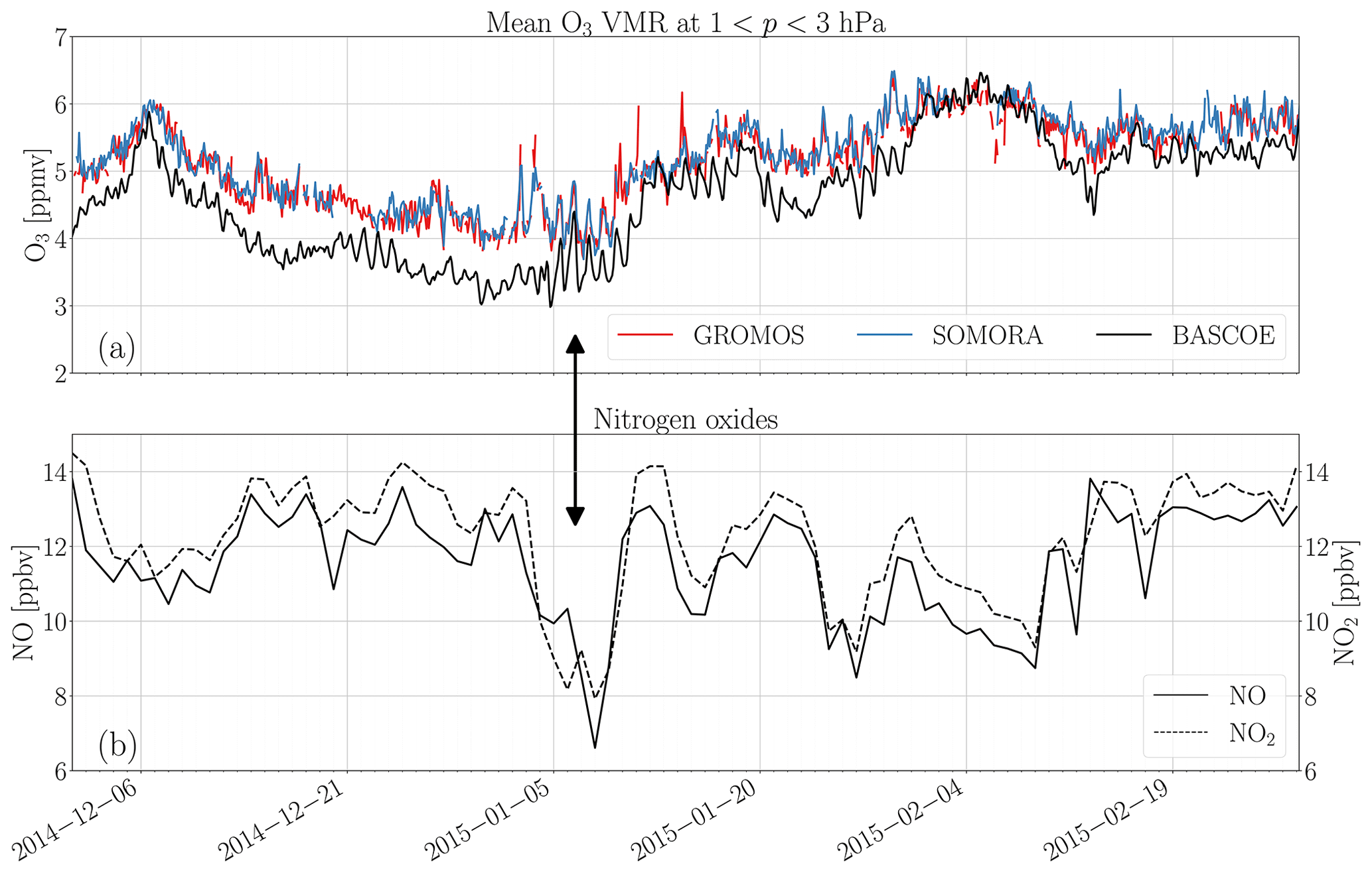
Figure 9(a) Ozone VMR from GROMOS, SOMORA, and BASCOE during the boreal winter 2014–2015. (b) Nitrogen oxides (NO and NO2) simulated by BASCOE. All quantities are averaged between 3 and 1 hPa and the ozone time series over 2 h time periods. NOx values are shown as daily mean of nighttime (NO2) and daytime (NO) values, respectively. The arrow highlights the period with an enhanced diurnal cycle.
The upper panel in Fig. 9 shows the ozone concentration in the upper stratosphere from GROMOS, SOMORA, and BASCOE. From the ozone time series already, there are time periods where the ozone VMR shows some large fluctuations on a diurnal basis in a season where the mean ozone cycle is usually small (see Fig. 6, around 40 km). An example of such a case can be seen at the beginning of January 2015 (arrow in Fig. 9) or, for instance, at the end of January 2015. From the BASCOE time series, we can even identify other periods with enhanced cycles, which are not really seen as such in the MWR measurements. These are some examples of what we refer to as “short-term ozone diurnal cycle variability”, generally lasting for a few days.
These enhancements can be better seen in Fig. 10, in the form of day-to-night anomalies in the middle atmosphere (60–0.1 hPa). It shows similar patterns in GROMOS and SOMORA time series, with a large increase in of around 1 hPa at the beginning of January 2015, followed by a secondary peak in the second half of the month. To some extent, BASCOE is also able to reproduce these two peaks in the ozone diurnal cycle, somehow limited to below 1 hPa and with limited vertical resolution.
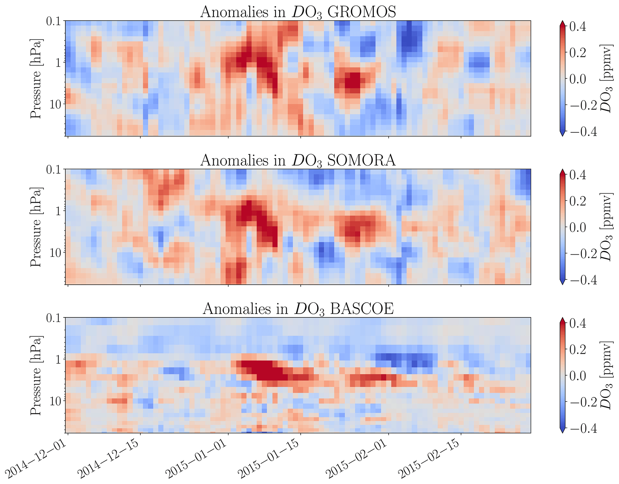
Figure 10Anomalies in day–night from GROMOS, SOMORA, and BASCOE during the boreal winter 2014–2015. For each dataset, we show the differences of compared to a monthly climatology computed on the decade 2010–2020.
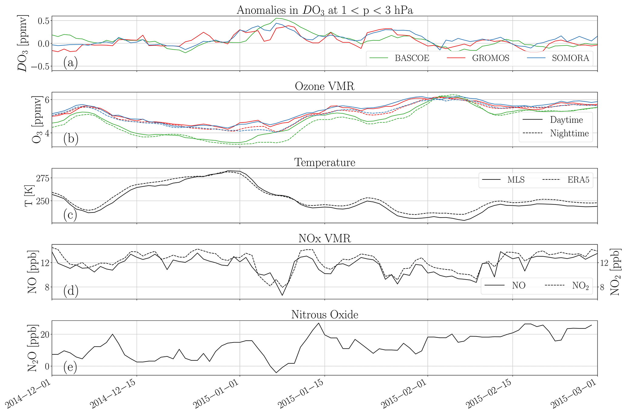
Figure 11Time series of different quantities during the winter 2014–2015, all averaged between 3 and 1 hPa. Panel (a) shows the anomalies, panel (b) shows the ozone VMR of the three dataset during daytime and nighttime, panel (c) shows temperature from MLS and ERA5, panel (d) shows NO and NO2 as simulated by BASCOE, and panel (e) shows N2O measurements from MLS.
Focusing on the upper stratosphere (3–1 hPa) where the anomalies are highest, Fig. 11 shows the temporal evolution of different quantities during the winter 2014–2015. In particular, Fig. 11b shows the day and nighttime ozone values. Focusing on the early January event, it can be seen that there is a consistent increase in daytime ozone from the three datasets, somehow delayed slightly in time in BASCOE compared to the MWRs. Such an increase is also visible during the second peak at the end of January for GROMOS and SOMORA and somehow less clearly in the BASCOE series. In terms of amplitude, this increase is substantial and corresponds approximately to 4 to 5 times the monthly averaged day-to-night difference in January, which is ∼0.1 ppmv at this pressure level.
Corresponding to these peaks in anomalies, sharp decreases in nitrogen oxides (NOx) are simulated from BASCOE. In fact, the decrease affects both nitric oxide (NO) and nitrogen dioxide (NO2). The two species are in photochemical balance during the day as NO mainly originates from photolysis of NO2 during daytime and can react with ozone to give back NO2, forming a major catalytic ozone depletion process in the middle atmosphere (Crutzen, 1970). In fact, the effect of NOx on ozone maximizes between 20 and 45 km altitude (∼50–1 hPa), corresponding well to the peaks of diurnal cycle enhancements seen in Fig. 10. To cross-validate these simulations, we also show some nitrous oxide (N2O) measurements taken by the MLS instrument on board the Aura satellite in Fig. 11e. Also here, the early January peak is visible as a decrease in the N2O measurement from MLS, which makes sense as N2O is the main source of NOx in this altitude region (McElroy and McConnell, 1971). Note that this is not the only event identified where such a behaviour can be seen. In fact, it seems that most winters seem to experience similar events (see, for example, similar plots for the boreal winter 2016–2017 shown in Appendix C).
In order to provide a more global picture and investigate the reasons for the N2O decrease seen above central Europe in the MLS measurements, we investigated the dynamical situation of the Northern Hemisphere by looking at the ERA5 reanalysis data during this period. In fact, this event follows closely a sudden stratospheric warming (SSW) which took place in early January. It was a minor warming but with significant disturbances on middle-atmospheric chemistry and transport (Manney et al., 2015). In fact, Fig. 2 from Manney et al. (2015) shows how the polar vortex briefly split at the onset of the SSW, leading to a mixing of the air between the mid-latitudes and the poles in the upper stratosphere. Following this event, some filaments of polar air containing little ozone and N2O reached central Europe as can be seen on the ozone map in Fig. 12. Such an irruption of polar air over Switzerland would explain the decrease in the N2O MLS measurements seen in early January and might well explain the subsequent changes in NOx and consequently in the ozone diurnal cycle.
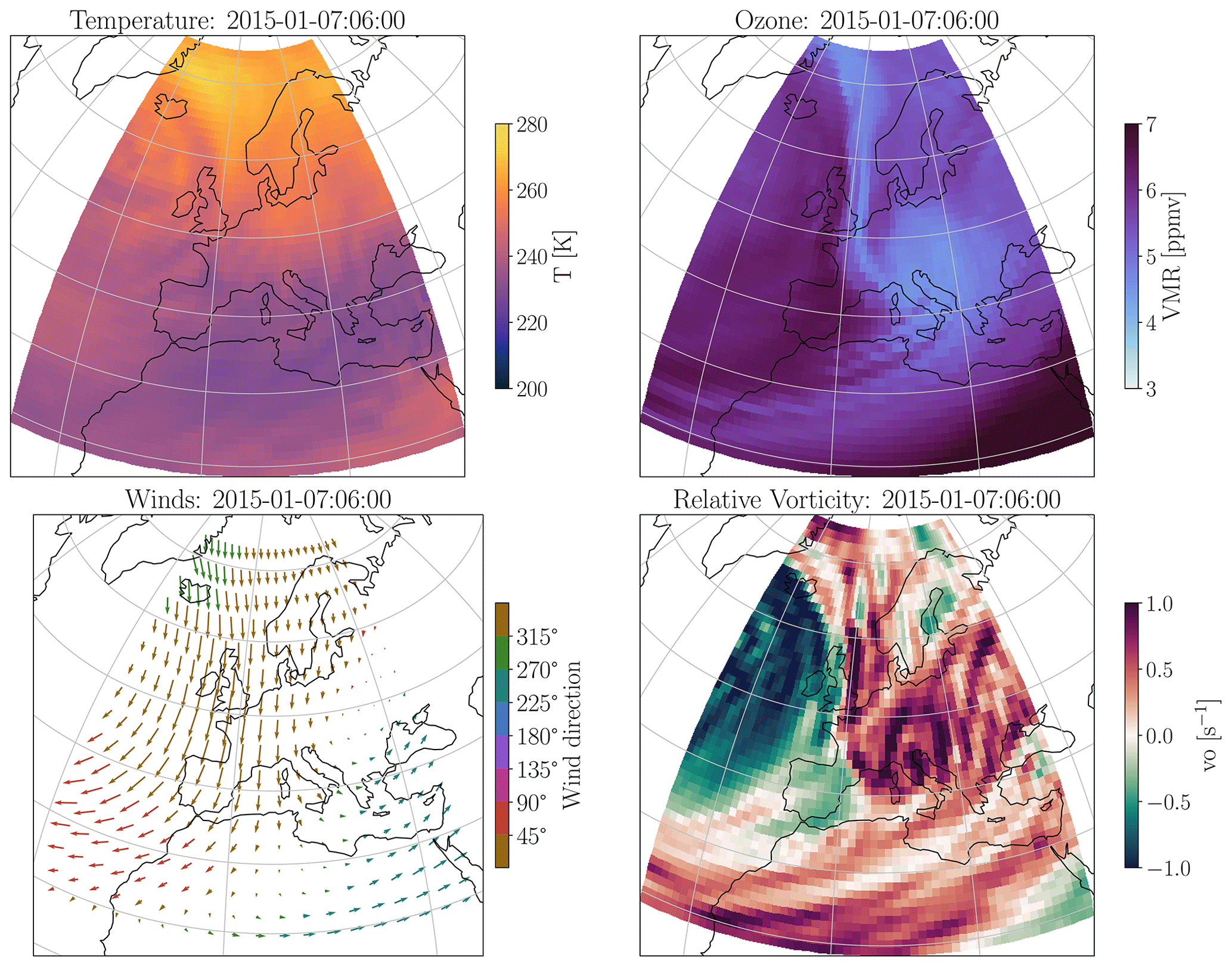
Figure 12Situation over Europe in the upper stratosphere ∼5 hPa shortly after the minor SSW of early January 2015 as seen in the ERA5 reanalysis.
Interestingly, we do not observe the strong ozone decrease associated with this filament of polar air reaching Bern, neither in the MWRs nor in the BASCOE time series. This could be a problem from the ERA5 reanalysis data as they do not feature any diurnal cycle at these altitudes and therefore might also lack the reaction of ozone to greater sun illumination (resulting in more ozone production and therefore increasing ozone amount in the low-ozone polar air which would be missed by the model). Even though this event might be considered a textbook example of such a dynamical event, we find it interesting to find such a coherent picture of a short-term event from a combination of ground-based measurements, chemistry transport model, satellite measurements, and reanalysis data.
In this publication, we focused on a specific case of short-term diurnal cycle variability related to NOx changes in the upper stratosphere. However, in the MWRs and in the BASCOE time series, the short-term variability is not always associated with changes in NOx concentration. Among the non-chemical processes that can impact the diurnal cycle amplitude, solar tides are important, both through vertical transport of Ox and through their modulation of temperature which can have a significant impact on ozone photochemistry (Schanz et al., 2014). Solar tides have periods of 1 solar day (24 h) or of its harmonics (e.g. 12 or 8 h) and can therefore impact the diurnal cycle as well, but generally their impact should be larger in the upper mesosphere and above (see, for example, Bjarnason et al., 1987; Huang et al., 2010b). However, Sakazaki et al. (2013) reported significant influence from tidal vertical transport at ∼35 km already; therefore, short-term tidal variability could induce some short-term variations of the ozone diurnal cycle in the upper stratosphere. The reciprocal is also true as variability of the stratospheric ozone thermal forcing can influence the generation of tides (Goncharenko et al., 2012). There have been studies on the tidal variability in the middle atmosphere, and it has been shown that solar tides are subject to a wide range of temporal variability, from intra-seasonal to short-term variability of a few days (Kopp et al., 2015; Baumgarten et al., 2018). It has also been shown that tides respond to SSW and can have non-linear interactions with planetary and gravity waves. Hence, it is likely that a coupling exists between the tidal variability and the short-term variability observed in the ozone diurnal cycle, but it is difficult to conclude on any causal relation without additional data (e.g. high-resolution temperature or wind measurements).
Using new harmonized ozone time series from two nearby microwave radiometers enables us to study in great detail the ozone diurnal cycle over Switzerland. With more than 11 years of parallel, independent measurements, these instruments provide a unique validation source for satellite and model-based datasets. We find that the recently published GDOC climatology compares well with our MWRs above Switzerland and agrees well with the WACCM and BASCOE models in the stratosphere and lower mesosphere. As reported by previous studies, we observe some remaining discrepancies between our observations and the models near the stratopause, in the transition region between ozone daytime accumulation and depletion. The discrepancies remain small and are significant only during summertime, where the diurnal cycle is stronger, providing better signal-to-noise ratio for the observations. Some of our results contradict a previous study also based on the GROMOS instrument (Studer et al., 2014), now providing a better agreement of the ozone diurnal cycle compared to model-based datasets but also compared to another previous MWR diurnal cycle study (Parrish et al., 2014). These updated results motivated the present study, and they are a consequence of the spectrometer change and of the recent harmonization of the calibration and retrieval routines of GROMOS and SOMORA (Sauvageat et al., 2022b).
For the first time, short-term variations of the ozone diurnal cycle could be detected in two co-located MWR time series, highlighting the value of ground-based radiometric measurements to monitor the short-term dynamics and photochemistry in the middle atmosphere. The quantification of these variations is limited by the rapidly increasing measurement noise; however, some enhancements of the diurnal cycle are clearly visible in the upper stratosphere during wintertime, where the diurnal cycle is otherwise very small. Compared to the averaged monthly diurnal cycle, we find an enhancement of 4–5 times the monthly mean diurnal cycle amplitude lasting for a few days. In fact, the observed short-term variability of the ozone diurnal cycle seems much higher than its intra-seasonal (month-to-month) or inter-annual variability during wintertime.
Regional (longitudinal) variability of the stratospheric ozone diurnal cycle has previously been identified by Schanz et al. (2014) in a model-based study from WACCM. They attributed the regional variability to changes in temperature (atmospheric tides), Ox, and NOy. Our study supports that, in some cases, short-term variability in the ozone diurnal cycle can be attributed to changes in NOx concentrations through dynamical transport. In other cases, other processes might be acting to modify the amplitude of the ozone diurnal cycle, e.g. changes in atmospheric tides. Our study also shows that a CTM like BASCOE is able to simulate the changes in the ozone diurnal cycle amplitude due to changes in NOx. In view of its significance, we believe that the reasons and importance of the short-term variability of the diurnal cycle should be further investigated globally with BASCOE.
It is beyond the scope of this publication to provide comprehensive analysis of this phenomenon, but we aim at bringing some new data to better understand stratospheric ozone diurnal cycle variability. It seems to be of particular interest in views of the recent studies aiming at better accounting for the stratospheric ozone diurnal variability in satellite datasets (e.g. Frith et al., 2020; Strode et al., 2022; Natarajan et al., 2023). Note that we focused our analysis on the upper stratosphere, where the short-term variability was most visible in our observations, but short-term variations are not limited to this region. In fact, our observations indicate that the variability is also present in the mesosphere and the lower stratosphere, where the role of NOx is less important and where other processes likely dominate. To conclude, more work is definitely needed to assess the importance of the short-term variability of the ozone diurnal cycle and confirm the potential role of other mechanisms influencing it.
C1 Short-term
In this section, we show measurements and simulations of the short-term variability during the boreal winter 2016–2017. Although more work is needed to unravel the complete picture of this winter, it shows another example of diurnal cycle enhancement associated with a sharp decrease in nitrogen oxides in the upper stratosphere.
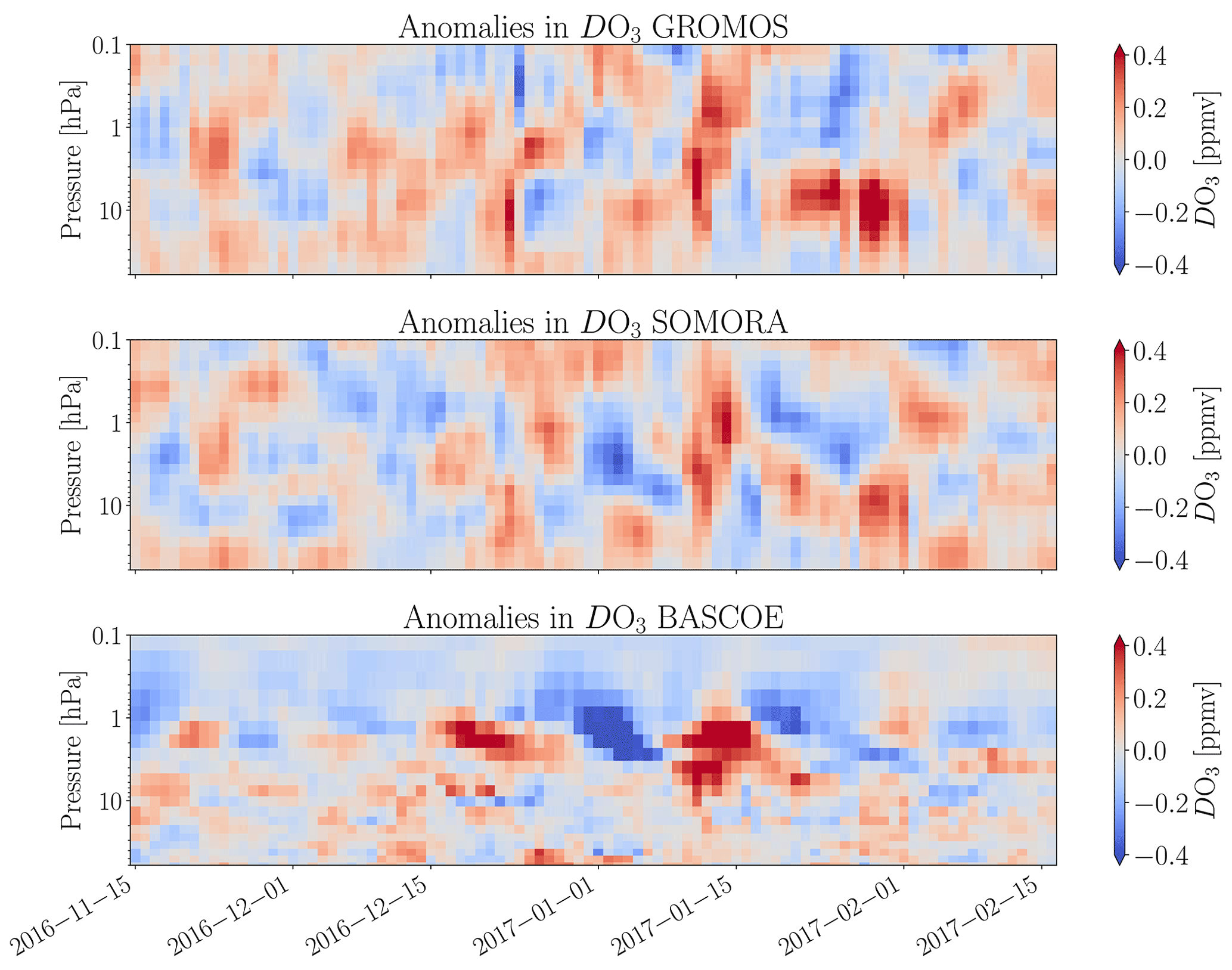
Figure C1Anomalies in day–night from GROMOS, SOMORA, and BASCOE during the boreal winter 2016–2017. For each dataset, we show the differences of compared to a monthly climatology computed on the decade 2010–2020.
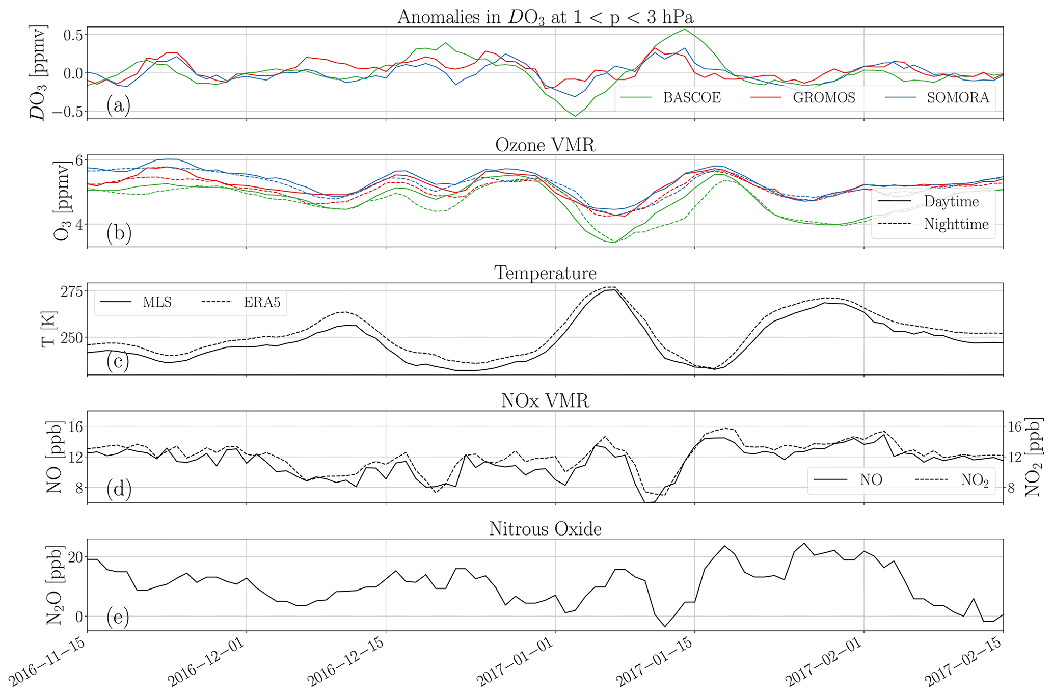
Figure C2Time series of different quantities during the winter 2016–2017, all averaged between 3 and 1 hPa. Panel (a) shows the anomalies, panel (b) shows the ozone VMR of the three dataset during daytime and nighttime, panel (c) shows temperature from MLS and ERA5, panel (d) shows NO and NO2 as simulated by BASCOE, and panel (e) shows N2O measurements from MLS.
The GROMOS and SOMORA level-2 data are available from the Bern Open Repository and Information System in the form of yearly netCDF files (https://doi.org/10.48620/65, Sauvageat et al., 2022a; https://doi.org/10.48620/119, Maillard Barras et al., 2022b). The recently harmonized calibration and retrieval routines are freely available at https://doi.org/10.5281/zenodo.6799357 (Sauvageat, 2022). The data and analysis code reproducing the results presented in this paper are freely available. MLS v5 data (Schwartz et al., 2020) are available from the NASA Goddard Space Flight Center Earth Sciences Data and Information Services Center (GES DISC): https://doi.org/10.5067/Aura/MLS/DATA2516. The ERA5 dataset (https://doi.org/10.24381/cds.143582cf, Hersbach et al., 2020, 2017) was downloaded from the Copernicus Climate Change Service (C3S) Climate Data Store. The CMIP6 recommendations for sulfate aerosols used in BASCOE are available at ftp://iacftp.ethz.ch/pub_read/luo/CMIP6/ (last access: 27 June 2023).
The supplement related to this article is available online at: https://doi.org/10.5194/acp-23-7321-2023-supplement.
ES carried out the data analysis, analysed the results, and prepared the manuscript. KH conceived the project and contributed to the interpretation of the results. EMB provided the SOMORA data and contributed to the interpretation of the results. SH performed a preliminary study within the frame of his Master's thesis. QE performed the BASCOE simulation and provided valuable help on the interpretation of all model results. AH and AM contributed to the interpretation of the results. All of the authors discussed the scientific findings and provided valuable feedback for the manuscript editing.
The contact author has declared that none of the authors has any competing interests.
Publisher’s note: Copernicus Publications remains neutral with regard to jurisdictional claims in published maps and institutional affiliations.
This article is part of the special issue “Atmospheric ozone and related species in the early 2020s: latest results and trends (ACP/AMT inter-journal SI)”. It is not associated with a conference.
The authors would like to acknowledge all the people involved in the design and operation of GROMOS and SOMORA. Also, they would like to thank the developers of the Atmospheric Radiative Transfer Simulator (Buehler et al., 2018), version 2.4 and their precious support to set up the ozone retrievals. In addition, we thank the numerous contributors to the free and open source software packages used for the data analysis, in particular xarray, matplotlib, Typhon and pyretrieval.
This work has been supported by MeteoSwiss and the Swiss Global Atmospheric Watch programme.
This paper was edited by Farahnaz Khosrawi and reviewed by two anonymous referees.
Ball, W. T., Alsing, J., Mortlock, D. J., Staehelin, J., Haigh, J. D., Peter, T., Tummon, F., Stübi, R., Stenke, A., Anderson, J., Bourassa, A., Davis, S. M., Degenstein, D., Frith, S., Froidevaux, L., Roth, C., Sofieva, V., Wang, R., Wild, J., Yu, P., Ziemke, J. R., and Rozanov, E. V.: Evidence for a continuous decline in lower stratospheric ozone offsetting ozone layer recovery, Atmos. Chem. Phys., 18, 1379–1394, https://doi.org/10.5194/acp-18-1379-2018, 2018. a
Baumgarten, K., Gerding, M., Baumgarten, G., and Lübken, F.-J.: Temporal variability of tidal and gravity waves during a record long 10-day continuous lidar sounding, Atmos. Chem. Phys., 18, 371–384, https://doi.org/10.5194/acp-18-371-2018, 2018. a
Bernet, L., von Clarmann, T., Godin-Beekmann, S., Ancellet, G., Maillard Barras, E., Stübi, R., Steinbrecht, W., Kämpfer, N., and Hocke, K.: Ground-based ozone profiles over central Europe: incorporating anomalous observations into the analysis of stratospheric ozone trends, Atmos. Chem. Phys., 19, 4289–4309, https://doi.org/10.5194/acp-19-4289-2019, 2019. a
Bhartia, P. K., McPeters, R. D., Flynn, L. E., Taylor, S., Kramarova, N. A., Frith, S., Fisher, B., and DeLand, M.: Solar Backscatter UV (SBUV) total ozone and profile algorithm, Atmos. Meas. Tech., 6, 2533–2548, https://doi.org/10.5194/amt-6-2533-2013, 2013. a
Bjarnason, G. G., Solomon, S., and Garcia, R. R.: Tidal influences on vertical diffusion and diurnal variability of ozone in the mesosphere, J. Geophys. Res.-Atmos., 92, 5609–5620, https://doi.org/10.1029/JD092iD05p05609, 1987. a
Buehler, S. A., Mendrok, J., Eriksson, P., Perrin, A., Larsson, R., and Lemke, O.: ARTS, the Atmospheric Radiative Transfer Simulator – version 2.2, the planetary toolbox edition, Geosci. Model Dev., 11, 1537–1556, https://doi.org/10.5194/gmd-11-1537-2018, 2018. a
Chabrillat, S., Vigouroux, C., Christophe, Y., Engel, A., Errera, Q., Minganti, D., Monge-Sanz, B. M., Segers, A., and Mahieu, E.: Comparison of mean age of air in five reanalyses using the BASCOE transport model, Atmos. Chem. Phys., 18, 14715–14735, https://doi.org/10.5194/acp-18-14715-2018, 2018. a
Chapman, S.: A theory of the upper-atmospheric ozone, Memoirs of the Royal Meteorological Society, 3, https://www.rmets.org/sites/default/files/papers/chapman-memoirs.pdf (last access: 27 June 2023), 1930. a
Connor, B. J., Siskind, D. E., Tsou, J., Parrish, A., and Remsberg, E. E.: Ground-based microwave observations of ozone in the upper stratosphere and mesosphere, J. Geophys. Res.-Atmos., 99, 16757–16770, https://doi.org/10.1029/94JD01153, 1994. a, b
Crutzen, P. J.: The influence of nitrogen oxides on the atmospheric ozone content, Q. J. Roy. Meteor. Soc., 96, 320–325, https://doi.org/10.1002/qj.49709640815, 1970. a, b
Errera, Q. and Fonteyn, D.: Four-dimensional variational chemical assimilation of CRISTA stratospheric measurements, J. Geophys. Res.-Atmos., 106, 12253–12265, https://doi.org/10.1029/2001JD900010, 2001. a
Errera, Q., Daerden, F., Chabrillat, S., Lambert, J. C., Lahoz, W. A., Viscardy, S., Bonjean, S., and Fonteyn, D.: 4D-Var assimilation of MIPAS chemical observations: ozone and nitrogen dioxide analyses, Atmos. Chem. Phys., 8, 6169–6187, https://doi.org/10.5194/acp-8-6169-2008, 2008. a, b
Frith, S. M., Bhartia, P. K., Oman, L. D., Kramarova, N. A., McPeters, R. D., and Labow, G. J.: Model-based climatology of diurnal variability in stratospheric ozone as a data analysis tool, Atmos. Meas. Tech., 13, 2733–2749, https://doi.org/10.5194/amt-13-2733-2020, 2020. a, b, c, d, e, f, g, h
Froidevaux, L., Jiang, Y. B., Lambert, A., Livesey, N. J., Read, W. G., Waters, J. W., Browell, E. V., Hair, J. W., Avery, M. A., McGee, T. J., Twigg, L. W., Sumnicht, G. K., Jucks, K. W., Margitan, J. J., Sen, B., Stachnik, R. A., Toon, G. C., Bernath, P. F., Boone, C. D., Walker, K. A., Filipiak, M. J., Harwood, R. S., Fuller, R. A., Manney, G. L., Schwartz, M. J., Daffer, W. H., Drouin, B. J., Cofield, R. E., Cuddy, D. T., Jarnot, R. F., Knosp, B. W., Perun, V. S., Snyder, W. V., Stek, P. C., Thurstans, R. P., and Wagner, P. A.: Validation of Aura Microwave Limb Sounder stratospheric ozone measurements, J. Geophys. Res.-Atmos., 113, D15S20, https://doi.org/10.1029/2007JD008771, 2008. a
Garcia, R. R., Marsh, D. R., Kinnison, D. E., Boville, B. A., and Sassi, F.: Simulation of secular trends in the middle atmosphere, 1950–2003, J. Geophys. Res.-Atmos., 112, D09301, https://doi.org/10.1029/2006JD007485, 2007. a
Godin-Beekmann, S., Azouz, N., Sofieva, V. F., Hubert, D., Petropavlovskikh, I., Effertz, P., Ancellet, G., Degenstein, D. A., Zawada, D., Froidevaux, L., Frith, S., Wild, J., Davis, S., Steinbrecht, W., Leblanc, T., Querel, R., Tourpali, K., Damadeo, R., Maillard Barras, E., Stübi, R., Vigouroux, C., Arosio, C., Nedoluha, G., Boyd, I., Van Malderen, R., Mahieu, E., Smale, D., and Sussmann, R.: Updated trends of the stratospheric ozone vertical distribution in the 60° S–60° N latitude range based on the LOTUS regression model , Atmos. Chem. Phys., 22, 11657–11673, https://doi.org/10.5194/acp-22-11657-2022, 2022. a
Goncharenko, L. P., Coster, A. J., Plumb, R. A., and Domeisen, D. I. V.: The potential role of stratospheric ozone in the stratosphere-ionosphere coupling during stratospheric warmings, Geophys. Res. Lett., 39, L08101, https://doi.org/10.1029/2012GL051261, 2012. a
Haefele, A., Hocke, K., Kämpfer, N., Keckhut, P., Marchand, M., Bekki, S., Morel, B., Egorova, T., and Rozanov, E.: Diurnal changes in middle atmospheric H2O and O3: Observations in the Alpine region and climate models, J. Geophys. Res.-Atmos., 113, D17303, https://doi.org/10.1029/2008JD009892, 2008. a, b, c
Hersbach, H., Bell, B., Berrisford, P., Hirahara, S., Horányi, A., Muñoz‐Sabater, J., Nicolas, J., Peubey, C., Radu, R., Schepers, D., Simmons, A., Soci, C., Abdalla, S., Abellan, X., Balsamo, G., Bechtold, P., Biavati, G., Bidlot, J., Bonavita, M., De Chiara, G., Dahlgren, P., Dee, D., Diamantakis, M., Dragani, R., Flemming, J., Forbes, R., Fuentes, M., Geer, A., Haimberger, L., Healy, S., Hogan, R.J., Hólm, E., Janisková, M., Keeley, S., Laloyaux, P., Lopez, P., Lupu, C., Radnoti, G., de Rosnay, P., Rozum, I., Vamborg, F., Villaume, S., and Thépaut, J.-N.: Complete ERA5 from 1940: Fifth generation of ECMWF atmospheric reanalyses of the global climate, Copernicus Climate Change Service (C3S) Data Store (CDS) [data set], https://doi.org/10.24381/cds.143582cf, 2017. a
Hersbach, H., Bell, B., Berrisford, P., Hirahara, S., Horányi, A., Muñoz-Sabater, J., Nicolas, J., Peubey, C., Radu, R., Schepers, D., Simmons, A., Soci, C., Abdalla, S., Abellan, X., Balsamo, G., Bechtold, P., Biavati, G., Bidlot, J., Bonavita, M., De Chiara, G., Dahlgren, P., Dee, D., Diamantakis, M., Dragani, R., Flemming, J., Forbes, R., Fuentes, M., Geer, A., Haimberger, L., Healy, S., Hogan, R. J., Hólm, E., Janisková, M., Keeley, S., Laloyaux, P., Lopez, P., Lupu, C., Radnoti, G., de Rosnay, P., Rozum, I., Vamborg, F., Villaume, S., and Thépaut, J.-N.: The ERA5 global reanalysis, Q. J. Roy. Meteor. Soc., 146, 1999–2049, https://doi.org/10.1002/qj.3803, 2020. a, b, c, d
Huang, F. T., Reber, C. A., and Austin, J.: Ozone diurnal variations observed by UARS and their model simulation, J. Geophys. Res.-Atmos., 102, 12971–12985, https://doi.org/10.1029/97JD00461, 1997. a
Huang, F. T., Mayr, H. G., Russell III, J. M., and Mlynczak, M. G.: Ozone diurnal variations in the stratosphere and lower mesosphere, based on measurements from SABER on TIMED, J. Geophys. Res.-Atmos., 115, D24308, https://doi.org/10.1029/2010JD014484, 2010a. a
Huang, F. T., McPeters, R. D., Bhartia, P. K., Mayr, H. G., Frith, S. M., Russell III, J. M., and Mlynczak, M. G.: Temperature diurnal variations (migrating tides) in the stratosphere and lower mesosphere based on measurements from SABER on TIMED, J. Geophys. Res.-Atmos., 115, D16121, https://doi.org/10.1029/2009JD013698, 2010b. a
Huijnen, V., Flemming, J., Chabrillat, S., Errera, Q., Christophe, Y., Blechschmidt, A.-M., Richter, A., and Eskes, H.: C-IFS-CB05-BASCOE: stratospheric chemistry in the Integrated Forecasting System of ECMWF, Geosci. Model Dev., 9, 3071–3091, https://doi.org/10.5194/gmd-9-3071-2016, 2016. a
Kinnison, D. E., Brasseur, G. P., Walters, S., Garcia, R. R., Marsh, D. R., Sassi, F., Harvey, V. L., Randall, C. E., Emmons, L., Lamarque, J. F., Hess, P., Orlando, J. J., Tie, X. X., Randel, W., Pan, L. L., Gettelman, A., Granier, C., Diehl, T., Niemeierm U., and Simmons, A. J.: Sensitivity of chemical tracers to meteorological parameters in the MOZART-3 chemical transport model, J. Geophys. Res.-Atmos., 112, D20302, https://doi.org/10.1029/2006JD007879, 2007. a
Kopp, M., Gerding, M., Höffner, J., and Lübken, F.-J.: Tidal signatures in temperatures derived from daylight lidar soundings above Kühlungsborn (54∘ N, 12∘ E), J. Atmos. Sol.-Terr. Phy., 127, 37–50, https://doi.org/10.1016/j.jastp.2014.09.002, 2015. a
Livesey, N. J., Read, W. G., Wagner, P. A., Froidevaux, L., Santee, M. L., Schwartz, M. J., Lambert, A., Valle, L. F. M., Pumphrey, H. C., Manney, G. L., Fuller, R. A., Jarnot, R. F., Knosp, B. W., and Lay, R. R.: Earth Observing System (EOS) Aura Microwave Limb Sounder (MLS) Version 5.0x Level 2 and 3 data quality and description document., Tech. Rep., https://mls.jpl.nasa.gov/eos-aura-mls/data-documentation, last access: 30 December 2022. a, b
Maillard Barras, E., Haefele, A., Nguyen, L., Tummon, F., Ball, W. T., Rozanov, E. V., Rüfenacht, R., Hocke, K., Bernet, L., Kämpfer, N., Nedoluha, G., and Boyd, I.: Study of the dependence of long-term stratospheric ozone trends on local solar time, Atmos. Chem. Phys., 20, 8453–8471, https://doi.org/10.5194/acp-20-8453-2020, 2020. a
Maillard Barras, E., Haefele, A., Stübi, R., Jouberton, A., Schill, H., Petropavlovskikh, I., Miyagawa, K., Stanek, M., and Froidevaux, L.: Dynamical linear modeling estimates of long-term ozone trends from homogenized Dobson Umkehr profiles at Arosa/Davos, Switzerland, Atmos. Chem. Phys., 22, 14283–14302, https://doi.org/10.5194/acp-22-14283-2022, 2022a. a
Maillard Barras, E., Sauvageat, E., Hocke, K., Murk, A., and Haefele, A.: Harmonized middle atmospheric ozone time series from SOMORA, BORIS Portal [data set], https://doi.org/10.48620/119, 2022b. a
Manney, G. L., Lawrence, Z. D., Santee, M. L., Read, W. G., Livesey, N. J., Lambert, A., Froidevaux, L., Pumphrey, H. C., and Schwartz, M. J.: A minor sudden stratospheric warming with a major impact: Transport and polar processing in the 2014/2015 Arctic winter, Geophys. Res. Lett., 42, 7808–7816, https://doi.org/10.1002/2015GL065864, 2015. a, b
Marsh, D. R., Mills, M. J., Kinnison, D. E., Lamarque, J.-F., Calvo, N., and Polvani, L. M.: Climate Change from 1850 to 2005 Simulated in CESM1(WACCM), J. Climate, 26, 7372–7391, https://doi.org/10.1175/JCLI-D-12-00558.1, 2013. a
McElroy, M. B. and McConnell, J. C.: Nitrous Oxide: A Natural Source of Stratospheric NO, J. Atmos. Sci., 28, 1095–1098, https://doi.org/10.1175/1520-0469(1971)028<1095:NOANSO>2.0.CO;2, 1971. a
Meinshausen, M., Vogel, E., Nauels, A., Lorbacher, K., Meinshausen, N., Etheridge, D. M., Fraser, P. J., Montzka, S. A., Rayner, P. J., Trudinger, C. M., Krummel, P. B., Beyerle, U., Canadell, J. G., Daniel, J. S., Enting, I. G., Law, R. M., Lunder, C. R., O'Doherty, S., Prinn, R. G., Reimann, S., Rubino, M., Velders, G. J. M., Vollmer, M. K., Wang, R. H. J., and Weiss, R.: Historical greenhouse gas concentrations for climate modelling (CMIP6), Geosci. Model Dev., 10, 2057–2116, https://doi.org/10.5194/gmd-10-2057-2017, 2017. a
Minganti, D., Chabrillat, S., Christophe, Y., Errera, Q., Abalos, M., Prignon, M., Kinnison, D. E., and Mahieu, E.: Climatological impact of the Brewer–Dobson circulation on the N2O budget in WACCM, a chemical reanalysis and a CTM driven by four dynamical reanalyses, Atmos. Chem. Phys., 20, 12609–12631, https://doi.org/10.5194/acp-20-12609-2020, 2020. a
Minganti, D., Chabrillat, S., Errera, Q., Prignon, M., Kinnison, D. E., Garcia, R. R., Abalos, M., Alsing, J., Schneider, M., Smale, D., Jones, N., and Mahieu, E.: Evaluation of the N2O Rate of Change to Understand the Stratospheric Brewer-Dobson Circulation in a Chemistry-Climate Model, J. Geophys. Res.-Atmos., 127, e2021JD036390, https://doi.org/10.1029/2021JD036390, 2022. a, b
Natarajan, M., Damadeo, R., and Flittner, D.: Solar occultation measurement of mesospheric ozone by SAGE III/ISS: impact of variations along the line of sight caused by photochemistry, Atmos. Meas. Tech., 16, 75–87, https://doi.org/10.5194/amt-16-75-2023, 2023. a
Orbe, C., Oman, L. D., Strahan, S. E., Waugh, D. W., Pawson, S., Takacs, L. L., and Molod, A. M.: Large-Scale Atmospheric Transport in GEOS Replay Simulations, J. Adv. Model. Earth Sy., 9, 2545–2560, https://doi.org/10.1002/2017MS001053, 2017. a
Pallister, R. C. and Tuck, A. F.: The diurnal variation of ozone in the upper stratosphere as a test of photochemical theory, Q. J. Roy. Meteor. Soc., 109, 271–284, https://doi.org/10.1002/qj.49710946002, 1983. a, b
Parrish, A., Boyd, I. S., Nedoluha, G. E., Bhartia, P. K., Frith, S. M., Kramarova, N. A., Connor, B. J., Bodeker, G. E., Froidevaux, L., Shiotani, M., and Sakazaki, T.: Diurnal variations of stratospheric ozone measured by ground-based microwave remote sensing at the Mauna Loa NDACC site: measurement validation and GEOSCCM model comparison, Atmos. Chem. Phys., 14, 7255–7272, https://doi.org/10.5194/acp-14-7255-2014, 2014. a, b, c, d, e, f
Prather, M. J.: Ozone in the upper stratosphere and mesosphere, J. Geophys. Res. 86, 5325, https://doi.org/10.1029/JC086iC06p05325, 1981. a
Prignon, M., Chabrillat, S., Friedrich, M., Smale, D., Strahan, S. E., Bernath, P. F., Chipperfield, M. P., Dhomse, S. S., Feng, W., Minganti, D., Servais, C., and Mahieu, E.: Stratospheric Fluorine as a Tracer of Circulation Changes: Comparison Between Infrared Remote-Sensing Observations and Simulations With Five Modern Reanalyses, J. Geophys. Res., 126, e2021JD034995, https://doi.org/10.1029/2021JD034995, 2021. a
Ricaud, P., Brillet, J., De La Noe, J., and Parisot, J. P.: Diurnal and seasonal variations of stratomesospheric ozone: Analysis of ground-based microwave measurements in Bordeaux, France, J. Geophys. Res.-Atmos., 96, 18617–18629, https://doi.org/10.1029/91JD01871, 1991. a
Rodgers, C. D. and Connor, B. J.: Intercomparison of remote sounding instruments, J. Geophys. Res.-Atmos., 108, 4116, https://doi.org/10.1029/2002JD002299, 2003. a
Sakazaki, T., Fujiwara, M., Mitsuda, C., Imai, K., Manago, N., Naito, Y., Nakamura, T., Akiyoshi, H., Kinnison, D., Sano, T., Suzuki, M., and Shiotani, M.: Diurnal ozone variations in the stratosphere revealed in observations from the Superconducting Submillimeter-Wave Limb-Emission Sounder (SMILES) on board the International Space Station (ISS), J. Geophys. Res.-Atmos., 118, 2991–3006, https://doi.org/10.1002/jgrd.50220, 2013. a, b
Sakazaki, T., Shiotani, M., Suzuki, M., Kinnison, D., Zawodny, J. M., McHugh, M., and Walker, K. A.: Sunset–sunrise difference in solar occultation ozone measurements (SAGE II, HALOE, and ACE–FTS) and its relationship to tidal vertical winds, Atmos. Chem. Phys., 15, 829–843, https://doi.org/10.5194/acp-15-829-2015, 2015. a
Sauvageat, E.: GROMORA-harmo: calibration and retrieval code for Swiss ozone microwave radiometers, version 2.0, Zenodo [code], https://doi.org/10.5281/zenodo.6799357, 2022. a
Sauvageat, E., Hocke, K., Maillard Barras, E., Haefele, A., and Murk, A.: Harmonized middle atmospheric ozone time series from GROMOS, BORIS Portal [data set], https://doi.org/10.48620/65, 2022a. a
Sauvageat, E., Maillard Barras, E., Hocke, K., Haefele, A., and Murk, A.: Harmonized retrieval of middle atmospheric ozone from two microwave radiometers in Switzerland, Atmos. Meas. Tech., 15, 6395–6417, https://doi.org/10.5194/amt-15-6395-2022, 2022b. a, b, c, d, e, f, g
Schanz, A., Hocke, K., and Kämpfer, N.: Daily ozone cycle in the stratosphere: global, regional and seasonal behaviour modelled with the Whole Atmosphere Community Climate Model, Atmos. Chem. Phys., 14, 7645–7663, https://doi.org/10.5194/acp-14-7645-2014, 2014. a, b, c
Schanz, A., Hocke, K., Kämpfer, N., Chabrillat, S., Inness, A., Palm, M., Notholt, J., Boyd, I., Parrish, A., and Kasai, Y.: The Diurnal Variation in Stratospheric Ozone from MACC Reanalysis, ERA-Interim, WACCM, and Earth Observation Data: Characteristics and Intercomparison, Atmosphere, 12, 625, https://doi.org/10.3390/atmos12050625, 2021. a, b
Schneider, N., Selsis, F., Urban, J., Lezeaux, O., Noé, J. D. L., and Ricaud, P.: Seasonal and Diurnal Ozone Variations: Observations and Modeling, J. Atmos. Chem., 50, 25–47, https://doi.org/10.1007/s10874-005-1172-z, 2005. a
Schranz, F., Fernandez, S., Kämpfer, N., and Palm, M.: Diurnal variation in middle-atmospheric ozone observed by ground-based microwave radiometry at Ny-Ålesund over 1 year, Atmos. Chem. Phys., 18, 4113–4130, https://doi.org/10.5194/acp-18-4113-2018, 2018. a, b
Schwartz, M., Froidevaux, L., Livesey, N., and Read, W.: MLS/Aura Level 2 Ozone (O3) Mixing Ratio V005, Goddard Earth Sciences Data and Information Services Center (GES DISC) [data set], https://doi.org/10.5067/Aura/MLS/DATA2516, 2020. a
Skachko, S., Ménard, R., Errera, Q., Christophe, Y., and Chabrillat, S.: EnKF and 4D-Var data assimilation with chemical transport model BASCOE (version 05.06), Geosci. Model Dev., 9, 2893–2908, https://doi.org/10.5194/gmd-9-2893-2016, 2016. a
SPARC: SPARC CCMVal Report on the Evaluation of Chemistry-Climate Models, in: SPARC Report, edited by: Eyring, V., Shepherd, T. G., and Waugh, D. W., SPARC Report No. 5, WCRP-30/2010, WMO/TD – No. 40, https://www.sparc-climate.org/publications/sparc-reports/ (last access: 27 June 2023), 2010. a
SPARC/IO3C/GAW: SPARC/IO3C/GAW Report on Long-term Ozone Trends and Uncertainties in the Stratosphere, in: SPARC Report, edited by: Petropavlovskikh, I., Godin-Beekmann, S., Hubert, D., Damadeo, R., Hassler, B., and Sofieva, V., SPARC Report No. 9, GAW Report No. 241, WCRP-17/2018, https://doi.org/10.17874/f899e57a20b, 2019. a
Strode, S. A., Taha, G., Oman, L. D., Damadeo, R., Flittner, D., Schoeberl, M., Sioris, C. E., and Stauffer, R.: SAGE III/ISS ozone and NO2 validation using diurnal scaling factors, Atmos. Meas. Tech., 15, 6145–6161, https://doi.org/10.5194/amt-15-6145-2022, 2022. a, b, c
Studer, S., Hocke, K., Schanz, A., Schmidt, H., and Kämpfer, N.: A climatology of the diurnal variations in stratospheric and mesospheric ozone over Bern, Switzerland, Atmos. Chem. Phys., 14, 5905–5919, https://doi.org/10.5194/acp-14-5905-2014, 2014. a, b, c, d, e, f
Vaughan, G.: Diurnal variation of mesospheric ozone, Nature, 296, 133–135, https://doi.org/10.1038/296133a0, 1982. a
Waters, J., Froidevaux, L., Harwood, R., Jarnot, R., Pickett, H., Read, W., Siegel, P., Cofield, R., Filipiak, M., Flower, D., Holden, J., Lau, G., Livesey, N., Manney, G., Pumphrey, H., Santee, M., Wu, D., Cuddy, D., Lay, R., Loo, M., Perun, V., Schwartz, M., Stek, P., Thurstans, R., Boyles, M., Chandra, K., Chavez, M., Chen, G.-S., Chudasama, B., Dodge, R., Fuller, R., Girard, M., Jiang, J., Jiang, Y., Knosp, B., LaBelle, R., Lam, J., Lee, K., Miller, D., Oswald, J., Patel, N., Pukala, D., Quintero, O., Scaff, D., Van Snyder, W., Tope, M., Wagner, P., and Walch, M.: The Earth observing system microwave limb sounder (EOS MLS) on the Aura Satellite, IEEE T. Geosci. Remote, 44, 1075–1092, https://doi.org/10.1109/TGRS.2006.873771, 2006. a, b
Zommerfelds, W. C., Kunzi, K. F., Summers, M. E., Bevilacqua, R. M., Strobel, D. F., Allen, M., and Sawchuck, W. J.: Diurnal variations of mesospheric ozone obtained by ground-based microwave radiometry, J. Geophys. Res.-Atmos., 94, 12819–12832, https://doi.org/10.1029/JD094iD10p12819, 1989. a, b
- Abstract
- Introduction
- Materials and methods
- Results and discussions
- Conclusions
- Appendix A: Monthly ozone profile comparisons
- Appendix B: Monthly diurnal cycle
- Appendix C: Short-term variability
- Code and data availability
- Author contributions
- Competing interests
- Disclaimer
- Special issue statement
- Acknowledgements
- Financial support
- Review statement
- References
- Supplement