the Creative Commons Attribution 4.0 License.
the Creative Commons Attribution 4.0 License.
 | 17 Jan 2023
How adequately are elevated moist layers represented in reanalysis and satellite observations?
Stefan A. Buehler
Manfred Brath
We assess the representation of elevated moist layers (EMLs) in ERA5 reanalysis, the Infrared Atmospheric Sounding Interferometer (IASI) L2 retrieval Climate Data Record (CDR) and the Atmospheric Infrared Sounder (AIRS)-based Community Long-term Infrared Microwave Combined Atmospheric Product System (CLIMCAPS)-Aqua L2 retrieval. EMLs are free-tropospheric moisture anomalies that typically occur in the vicinity of deep convection in the tropics. EMLs significantly affect the spatial structure of radiative heating, which is considered a key driver for meso-scale dynamics, in particular convective aggregation. To our knowledge, the representation of EMLs in the mentioned data products has not been explicitly studied – a gap we start to address in this work. We assess the different datasets' capability of capturing EMLs by collocating them with 2146 radiosondes launched from Manus Island within the western Pacific warm pool, a region where EMLs occur particularly often. We identify and characterise moisture anomalies in the collocated datasets in terms of moisture anomaly strength, vertical thickness and altitude. By comparing the distributions of these characteristics, we deduce what specific EML characteristics the datasets are capturing well and what they are missing. Distributions of ERA5 moisture anomaly characteristics match those of the radiosonde dataset quite well, and remaining biases can be removed by applying a 1 km moving average to the radiosonde profiles. We conclude that ERA5 is a suitable reference dataset for investigating EMLs. We find that the IASI L2 CDR is subject to stronger smoothing than ERA5, with moisture anomalies being on average 13 % weaker and 28 % thicker than collocated ERA5 anomalies. The CLIMCAPS L2 product shows significant biases in its mean vertical humidity structure compared to the other investigated datasets. These biases manifest as an underestimation of mean moist layer height of about 1.3 km compared to the three other datasets that yields a general mid-tropospheric moist bias and an upper-tropospheric dry bias. Aside from these biases, the CLIMCAPS L2 product shows a similar, if not better, capability of capturing EMLs compared to the IASI L2 CDR. More nuanced evaluations of CLIMCAPS' capabilities may be possible once the underlying cause for the identified biases has been found and fixed. Biases found in the all-sky scenes do not change significantly when limiting the analysis to clear-sky scenes. We calculate radiatively driven vertical velocities ωrad derived from longwave heating rates to estimate the dynamical effect of the moist layers. Moist-layer-associated ωrad values derived from Global Climate Observing System Reference Upper-Air Network (GRUAN) soundings range between 2 and 3 hPa h−1, while mean meso-scale pressure velocities from the EUREC4A (Elucidating the Role of Clouds-Circulation Coupling in Climate) field campaign range between 1 and 2 hPa h−1, highlighting the dynamical significance of EMLs. Subtle differences in the representation of moisture and temperature structures in ERA5 and the satellite datasets create large relative errors in ωrad on the order of 40 % to 80 % with reference to GRUAN, indicating limited usefulness of these datasets to assess the dynamical impact of EMLs.
- Article
(2890 KB) - Full-text XML
- BibTeX
- EndNote


The vertical structure of water vapour in the troposphere is a key driver for meso-scale processes, such as the development and maintenance of convective systems. In particular, it determines the vertical structure of radiative heating due to water vapour's strong ability to absorb and emit infrared (IR) radiation. The spatial structure of radiative heating in the vicinity of convection is capable of driving circulations that contribute to the maintenance of the convection (Muller and Bony, 2015; Wing et al., 2017; Schulz and Stevens, 2018; Muller et al., 2022). Hence, understanding the vertical structure of water vapour is key for our understanding of convective aggregation, which remains a large contributor of uncertainty to climate projections (Bony et al., 2015).
A common meso-scale phenomenon affecting the vertical humidity structure in the tropics is elevated moist layers (EMLs) in the lower troposphere to mid-troposphere, which frequently occur either in the vicinity of deep convection or in association with extratropical dry air intrusions (Villiger et al., 2022). EMLs can extend horizontally over several hundred kilometres and have lifetimes of about a day (Stevens et al., 2017; Johnson et al., 1996). In the convection-dominated regions near the Intertropical Convergence Zone (ITCZ), especially over the western Pacific warm pool, EMLs are particularly common and manifest as a secondary maximum of relative humidity (RH) in the climatological profile near the melting level at around 5 km altitude (Romps, 2014).
It is important to capture EMLs in observational and reanalysis datasets, which serve as reference for modelling studies (Lang et al., 2021; Eyring et al., 2016; Teixeira et al., 2014; Ferraro et al., 2015; Brands et al., 2013; Jiang et al., 2012). In particular, Lang et al. (2021) highlight the importance of reducing uncertainties in clear-sky mid-tropospheric humidity in global storm-resolving models that yield significant differences in the models' radiation budgets. Hence, having suitable global and long-term satellite and reanalysis datasets to assess such model differences is of great value.
In a case study, Stevens et al. (2017) found strong limitations of passive satellite-based humidity retrievals to resolve an EML, suggesting a somewhat fundamental EML blind spot for such observations. This is particularly surprising for the advanced hyperspectral IR instruments such as AIRS (Atmospheric Infrared Sounder) or IASI (Infrared Atmospheric Sounding Interferometer), which offer rich vertical information content about temperature and water vapour. In our recent study (Prange et al., 2021), we found a physical explanation for the apparent EML blind spot, suggesting that the limited temperature information available with the particular retrieval setup deployed by Stevens et al. (2017) is responsible for the inability to resolve the EML with IASI. In the same article, we showed that EMLs do not pose an inherent blind spot for hyperspectral IR retrievals based on simulated observations. In this work we follow up on our previous analysis with an evaluation of EMLs in operational hyperspectral IR retrieval products based on the IASI and AIRS instruments. With hyperspectral IR observations being a significant data contribution to reanalysis products (Cardinali, 2009; Dahoui et al., 2017, e.g.), we also assess EMLs in ERA5 (ECMWF Reanalysis v5). To our knowledge, EMLs have not been explicitly studied based on any of these data products. We start addressing this gap in this study by conducting an assessment of the one-dimensional vertical structure of EMLs based on reference data from the western Pacific warm pool region.
The western Pacific warm pool region is particularly suited to study EMLs because of the frequent occurrence of deep convection. Hence, as reference dataset we use the GRUAN (Global Climate Observing System Reference Upper-Air Network) radiosondes launched on Manus Island from 2011 to 2014. We collocate the datasets within 50 km in space and 30 min in time to make the data directly comparable. We first assess the mean profiles of humidity, temperature and static stability to quantify the mean atmospheric state in the study region for the different datasets. We then apply the moisture anomaly identification and characterisation method of Prange et al. (2021) to statistically quantify the EMLs of the collocated datasets. This method allows for a dedicated comparison of EML characteristics such as EML strength, thickness and height. It also enables a direct quantification of the moisture anomalies' effect on the radiative heating rate, the spatial structure of which is a key driver for the meso-scale dynamics of the atmosphere. We do this quantification by calculating moist-layer-associated radiatively driven vertical velocities, which we compare to meso-scale measurements of pressure velocities from the EUREC4A (Elucidating the Role of Clouds-Circulation Coupling in Climate) field campaign (Stevens et al., 2021).
We investigate the vertical moisture characteristics of GRUAN radiosonde data, ERA5 reanalysis and of two satellite retrieval products based on the IASI and AIRS instruments. We chose two retrieval datasets that have the scope of being useful for climate applications by applying long-term consistent algorithms. In contrast, operational retrieval algorithms meant for the near-real-time production of geophysical fields, such as IASI L2 or NUCAPS (NOAA Unique Combined Atmospheric Processing System), do not have the scope of being a consistent CDR (EUMETSAT, 2017; Berndt et al., 2020). In the following, we highlight the most important properties of these datasets for the context of this work. This includes brief descriptions of the datasets' spatial and temporal sampling characteristics, a brief summary of their underlying algorithms and our own processing steps. Figure 1 provides a spatial overview of the research region and the typical sampling over 1 d. Note that one processing step we apply to all datasets, except GRUAN, is to filter out data points over land to assure homogeneous surface conditions.
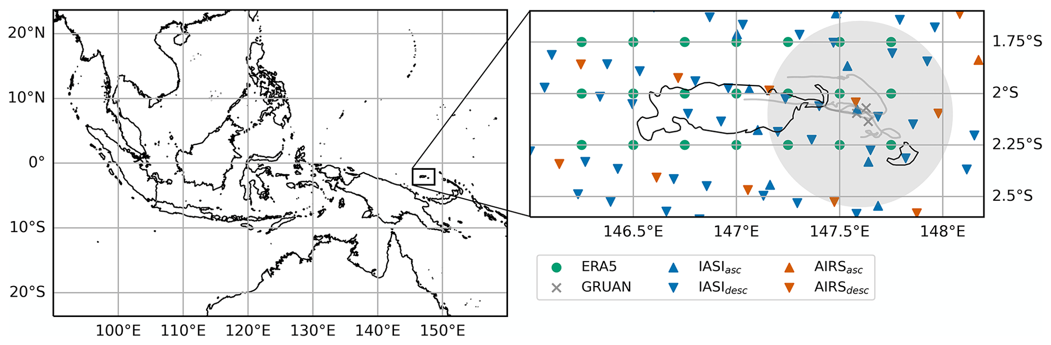
Figure 1Maps show the geographical location of Manus Island and spatial sampling over 1 d (28 March 2012) of the four investigated datasets. The satellite data are split into ascending and descending node data. Radiosonde pathways are shown as lines. Their mean position is indicated by grey crosses that are used as collocation locations. The transparent grey circle visually indicates the collocation radius of 50 km.
2.1 GRUAN radiosondes
The GRUAN (Global Climate Observing System Reference Upper-Air Network) measurement programme consists of a network of about 30 quality-controlled radiosonde measurement sites around the world to detect trends in essential climate variables such as temperature and humidity (Seidel et al., 2009; Dirksen et al., 2014). Here we pick out the GRUAN site on Manus Island, where radiosondes were launched from January 2011 to July 2014, run by the Atmospheric Radiation Measurement programme (Ackerman and Stokes, 2003). This is a particularly suited reference dataset for the scope of our work for two reasons. Firstly, Manus Island is located at about 2∘ S in the western Pacific warm pool, a region where EMLs are expected to occur frequently due to their link to deep convective events. Secondly, the standard radiosonde launch times at 00:00 and 12:00 UTC with a local time shift of UTC+10 h turn out to coincide well with IASI overpasses at the fixed Equator crossing time (ECT) of the Metop satellites at around 09:30 local time.
The GRUAN sounding data used in this work are obtained from the RS92-GDP.2 data archive. Uncertainty estimates are 6 % for relative humidity (RH) and between 0.15 and 0.6 K for temperature depending on daytime and altitude (Dirksen et al., 2014). When binning the launch times of the full sounding dataset into hourly intervals, about 60 % of the soundings occur around the 00:00 and 12:00 UTC launch times. A significant anomaly in radiosonde launch times occurred from 24 September 2011 to 31 March 2012 with launches every 3 h as part of the DYNAMO campaign (Yoneyama et al., 2013).
As a first step of preparing the GRUAN sounding data for our processing, relative humidity values are transformed from being defined with respect to the saturation vapour pressure above water (GRUAN standard) to a mixed phase approach as described by ECMWF (2018). We then linearly interpolate the sounding dataset to a fixed altitude grid ranging from 0 m at the surface to 15 km altitude at 10 m intervals. In the event of missing values in the original data, we interpolate over intervals of up to 100 m and leave the missing values for larger intervals. We then deduce H2O volume mixing ratios (VMRs) from RH, temperature and pressure.
2.2 ERA5
We use the ECMWF Reanalysis v5 (ERA5) high-resolution atmospheric data on a 31 km spaced horizontal grid, on 137 vertical levels and in hourly intervals. Detailed descriptions of spatial and temporal discretisation of ERA5 are provided in the overview paper and in the IFS (version Cy41r2) documentation (Hersbach et al., 2020; ECMWF, 2016).
We use a total of 21 ERA5 pixels around Manus Island as depicted in Fig. 1. The data are originally stored on a T639 spectral grid or a reduced Gaussian grid depending on the variable. We transform the grids of all variables to a 0.25∘ evenly spaced latitude–longitude grid using bilinear interpolation. We deduce H2O VMR as our main humidity quantity from the specific humidity that is originally provided in ERA5. We deduce altitudes for each ERA5 profile by assuming a hydrostatic atmosphere and using the fixed pressure grid and the temperature profiles as input.
2.3 IASI L2 Climate Data Record
The IASI Level 2 retrieval dataset used in this work is called the “IASI All Sky Temperature and Humidity Profiles – Climate Data Record Release 1.1 – Metop-A and -B” and is provided by EUMETSAT (2022). We use only data from Metop-A. We refer to this dataset as the IASI L2 CDR in the frame of this study. The dataset is aimed to be a consistently reprocessed long-term dataset based on the most recent version of the statistical piecewise linear regression (PWLR) EUMETSAT retrieval algorithm. Data of the near-real-time operational IASI L2 retrieval are subject to significant jumps over the years due to algorithm updates (EUMETSAT, 2017). Since the algorithm of the period between 2011 to 2014 is not representative of today's standard, we use the reprocessed IASI L2 CDR.
Details about the IASI L2 CDR are provided in the product user guide (EUMETSAT, 2022). Here we summarise some of its main properties. The retrieval algorithm makes use of IASI spectra and radiances observed by the microwave sounders AMSU-A (Advanced Microwave Sounding Unit-A) and MHS (Microwave Humidity Sounder) aboard the same satellite to also retrieve information about atmospheric temperature and humidity in the presence of clouds. The retrieval is conducted on the native pixel resolution of IASI with a pixel diameter of about 12 km at nadir. Only AMSU-A information is available on 2×2 arrays of IASI pixels. To train the PWLR retrieval algorithm, global sensing data of 4 d of each month of the years 2015 and 2016 are matched with ERA5 temperature, humidity and ozone profiles on 137 vertical levels. Cloudy scenes are included in the training step of the algorithm to allow for the retrieval of atmospheric quantities in all-sky scenes. The retrieval is conducted on 137 atmospheric levels and an additional surface level. All-sky retrievals are conducted for atmospheric temperature and specific humidity profiles as well as for surface temperature and total column water vapour. A cloud fraction estimate is also provided based on AVHRR (Advanced Very High Resolution Radiometer) data that are integrated over the retrieval's field of view. The dataset also comes with uncertainty estimates for temperature and humidity profile retrievals that reflect the mean uncertainty of the surface level and the mid-troposphere (EUMETSAT, 2022). These uncertainties are provided in units of kelvin in temperature and dew point temperature. As recommended in the user guide, we filter cases considered highly defective with uncertainties > 4 K. This filtering only removes about 1 % of data. We want to highlight that we repeated our analysis based on more strict filtering criteria with uncertainties < 1 K but found no significant changes to our results.
The only variable we add in our own processing is the height associated with the retrieval's vertical levels. For this purpose we assume a hydrostatic atmosphere and use profiles of pressure and temperature as input.
2.4 CLIMCAPS-Aqua L2 product
The Community Long-term Infrared Microwave Combined Atmospheric Product System (CLIMCAPS)-Aqua Level 2 product is based on AIRS spectra and AMSU-A radiances. The processing uses a sophisticated stepwise optimal estimation procedure following the formalism of Rodgers (2000) of various atmospheric quantities such as temperature, moisture, cloud heights and fractions, and concentrations of trace gas species O3, CO, CH4, CO2, HNO3 and SO2. The retrieval is conducted on about 50 km spatial pixels at nadir (150 km at scan edge). One pixel is referred to as field of regard (FOR) and is made up of 9 (3×3) AIRS field of views (FOVs). The retrieval procedure and a characterisation of retrieval errors are described by Smith and Barnet (2019). In an evaluation of the CLIMCAPS observing capability, it is found that CLIMCAPS has sensitivity to multiple narrow tropospheric layers in temperature and humidity – a promising premise for our study (Smith and Barnet, 2020).
We limit our use of available CLIMCAPS variables to the retrieved surface temperature, temperature and humidity profiles, the total cloud fraction, the geopotential height, and the respective quality control flags and error estimates. Temperature profiles are provided on 100 fixed vertical pressure levels from the surface to the top of atmosphere, and specific humidity profiles are provided on 66 levels from the surface to about 50 hPa. Since surface pressure is not a retrieval quantity and instead MERRA2 (Modern-Era Retrospective analysis for Research and Applications, Version 2) surface pressures are used as input to the retrieval, we calculate surface values of humidity following the boundary layer adjustment procedure that is described in the CLIMCAPS science application guide (Smith et al., 2021). Surface values of humidity are important for our method of analysing moisture anomaly characteristics that is described in Sect. 4.
The quality control flags are provided for each variable on all vertical levels. They subdivide the retrieval into “best”, “good” and “rejected” quality. We filter cases where the specific humidity quality control flag of the level closest to MERRA2 surface pressure is labelled “rejected” and cases with more than 10 “rejected” vertical levels in humidity between 900 and 100 hPa. These criteria are quite stringent as they filter about 90 % of the data. However, we do not aim to analyse data that are already flagged as being of deficient quality.
A significant difference between the IASI L2 product and the CLIMCAPS product lies in the estimation of the total cloud fraction and the way cloudy scenes are handled. While for the IASI L2 product cloud fraction is estimated based on an independent instrument (AVHRR), CLIMCAPS estimates cloud fraction based on a subset of cloud-sensitive AIRS channels. CLIMCAPS does so for each AIRS FOV and provides a derived FOR-integrated total cloud fraction, i.e. over 3×3 FOVs. To retrieve atmospheric quantities in cloudy conditions, the CLIMCAPS and IASI retrieval products deploy conceptually different methods. While the IASI product attempts retrieval through the cloud on the native IASI pixel size of 12 km, CLIMCAPS deploys a cloud-clearing technique where information from the 3×3 AIRS FOV spectra are combined to represent the atmospheric state around the clouds throughout the total retrieval FOR. For the IASI L2 CDR, a retrieval through the cloud can only be achieved through the water vapour and temperature information available from the microwave sounders since IR sounders do not yield information through clouds. We specifically compare the retrievals' capabilities to resolve vertical moisture structures in all-sky and clear-sky conditions in Sect. 5.1 and 5.2.
2.5 Collocation procedure
We collocate the datasets pairwise in space and time to seek high direct comparability of the investigated scenes. This is done using a collocation toolkit that is freely available as part of the “typhon” collection of Python functions for atmospheric science (https://www.radiativetransfer.org/tools/, last access: 3 January 2023). We want to highlight that direct comparability of the datasets is inherently limited due to different horizontal resolutions of the datasets in the presence of inhomogeneous atmospheric fields. By still comparing the datasets' vertical humidity structures directly, we implicitly assume that differences in the datasets’ effective vertical resolution are significantly higher than the averaging effect of different horizontal resolutions on the vertical moisture structure. We would argue that, if for any of the compared datasets, this assumption may break for some cases of point source GRUAN radiosonde comparisons to ERA5 or IASI/AIRS retrievals. However, as shown in Sect. 5.1, we find ERA5 to match EML characteristics of GRUAN quite well, indicating that horizontal resolution mismatches are not the significant error source in the conducted comparisons.
We conduct the collocation for four dataset pairs, namely ERA5/GRUAN, IASI/GRUAN, IASI/ERA5 and CLIMCAPS/ERA5. With GRUAN being the gold standard reference dataset, we use it as reference where sufficient collocations are available. The standard launch times at 00:00 UTC and 12:00 UTC in conjunction with a local time difference on Manus Island of UTC+10 h yield launches at local times of about 10:00 and 22:00, matching up well with the IASI Equator crossing time of about 09:30 and 21:30. Unfortunately for the AIRS-based CLIMCAPS retrieval, there is a systematic offset of about 4 h in GRUAN radiosonde launch time and the Equator crossing time of the Aqua satellite at around 01:30 and 13:30. We decide to choose rather conservative collocation criteria of 50 km and 30 min. The temporal criterion of 30 min is chosen due to the expected 30 min offset of IASI overpasses and regular radiosonde launches. In addition, 30 min assures temporal collocation with ERA5, which has hourly sampling. These collocation criteria still yield a high number of matches between IASI, GRUAN and ERA5 while disabling matches between CLIMCAPS and GRUAN. Although previous case studies of EMLs suggest EML lifetimes of about a day (e.g. Stevens et al., 2017; Villiger et al., 2022), we prefer to use quite strict collocation criteria since atmospheric variability over the course of hours can still be significant (Buehler et al., 2012). In addition, while retaining tight collocation criteria, we find that an evaluation of CLIMCAPS retrievals is still possible with respect to ERA5, which we find to represent EMLs reasonably well when compared to GRUAN (see Sect. 5.1).
For collocation pairs where the secondary dataset has higher spatial resolution than our spatial collocation radius of 50 km, several pixels of the secondary dataset can match with one pixel of the reference dataset. This is frequently the case for all collocation pairs because the lowest-resolution dataset CLIMCAPS has a 50 km pixel diameter while the collocation diameter is 100 km. In these cases, we randomly select one of the matching pixels. In cases where the spatial resolution of the reference dataset is higher than our spatial collocation radius, it can occur that the same data points of the collocated secondary dataset collocate with several data points in the reference dataset. This is the case for the collocations with reference to ERA5. We reject cases where the same data point of the secondary dataset would be used more than once to assure that all collocations are truly independent data pairs.
Applying the described collocation criteria and the dataset-specific filtering criteria described above, we obtain 1921 ERA5/GRUAN collocations, 648 IASI/GRUAN collocations, 37 491 IASI/ERA5 collocations and 2500 AIRS/ERA5 collocations. The strong discrepancy in the number of collocations has several reasons. First, matches with ERA5 within our collocation criteria are available for all data points of the other datasets, yielding a high number of collocations for every dataset with reference to ERA5. The reason for the number of IASI/ERA5 and AIRS/ERA5 collocations deviating significantly lies in the different reduction of data points in IASI and AIRS retrievals when applying the quality criteria described in Sects. 2.3 and 2.4.
To get a first overview of the vertical structure of humidity and temperature in the vicinity of Manus Island and possible biases between the different datasets, we take a look at the mean profiles over the 4 years of available data. Figure 2 shows (a) water vapour volume mixing ratio (H2O VMR), (b) relative humidity (RH), (c) the deviation of potential temperature (Θ) from a moist adiabat and (d) the static stability calculated as
Static stability describes the ability of an air mass at rest to become vertically laminar or turbulent due to effects of buoyancy. It is mainly controlled by the vertical gradient of temperature, where an increase with height corresponds to a stable stratification while a decrease with height corresponds to an unstable stratification. We use it here as a measure to better assess differences in temperature stratification of the data products, in particular near the melting level. In addition, static stability is used in Sect. 6 to transform radiative heating rate to vertical velocities, assuming a constant vertical temperature structure.
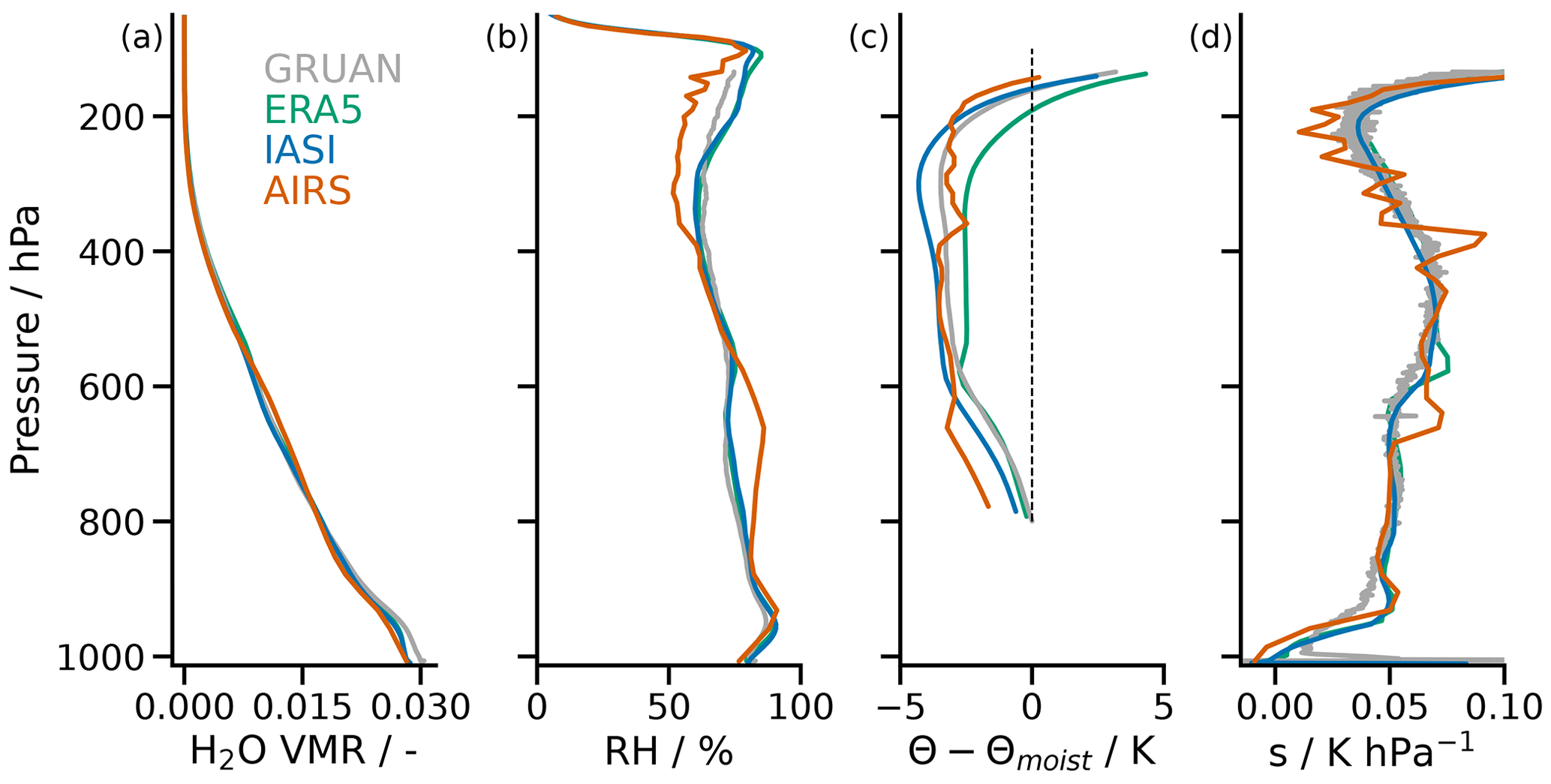
Figure 2Mean profiles of (a) H2O volume mixing ratio (VMR), (b) relative humidity (RH), (c) deviation of potential temperature (Θ) from moist adiabat (Θmoist) based on mean Θ at 700 hPa of GRUAN data and (d) the static stability s in the vicinity of Manus Island based on the four investigated datasets. Only collocated data with ERA5 are used. For the ERA5 profiles, collocated data with IASI are used.
Since all datasets can be collocated with ERA5 data, we base the analysis of the mean profiles on the collocation datasets with reference to ERA5 to assure good comparability. This leaves us with three different subsets of ERA5 data that collocate with the other respective data products. We investigated how the mean profiles of ERA5 vary among these subsets and find the variation to not be significant compared to differences between the data products (not shown). Hence, for the ERA5 mean profiles depicted in Fig. 2, we choose the collocations with reference to IASI since they contain the most cases.
The mean vertical humidity structure depicted in Fig. 2a and b shows the typical moist conditions throughout the troposphere that are expected in a deep convective region. RH values rarely drop below 70 % in any of the datasets. A trimodal vertical RH structure is apparent in all datasets with maxima near the surface, in the mid-troposphere and near the tropopause. This vertical structure is in line with previous studies of the vertical distribution of humidity, clouds and detrainment in the ITCZ region (Johnson et al., 1996, 1999; Mapes and Zuidema, 1996; Posselt et al., 2008; Romps, 2014). Here, we target the mid-tropospheric humidity structure as the primary research object, where the presence of an RH maximum highlights the climatological significance of EMLs in our research region.
Comparing the mean RH profiles of the different datasets, the particularly good agreement of ERA5 and IASI sticks out. Since the IASI L2 retrieval is trained based on ERA5 data, it is not surprising that the means of the two datasets are so similar. The additional good agreement with GRUAN shows that the datasets are not only self-consistent but also close to reference data. However, good agreement in the mean is not indicative of the datasets' capability to resolve vertical moisture variability, which we investigate separately in Sect. 5.1.
AIRS on the other side shows significant biases in RH against the other three datasets. The mid-tropospheric peak in RH is shifted towards a significantly lower altitude while the lower RH peak of the boundary layer is shifted a bit upwards. This yields a moist bias of AIRS between about 600 and 800 hPa. We view the vertical shift of the mid-tropospheric RH maximum to most likely not be caused by resolution-induced errors, with vertical resolution being estimated between 1 and 4 km for CLIMCAPS (Smith and Barnet, 2020). While for individual profiles limited vertical resolution may yield some error in the height of moisture features, we do not see how resolution-induced errors would yield a consistent downward shift of the mid-tropospheric RH maximum of more than 1 km that is evident in the mean profile. If at all, we would expect an upward shift in the mid-tropospheric RH maximum associated with this effect because vertical resolution is typically better in higher altitudes, which may cause a shift in a moisture anomaly's centre of mass upwards where there is less smoothing. As a possible reason to explain the altitude shifts in humidity features, we investigated whether mean humidity profiles are different when we deduce them from the original retrieval quantities, namely the column density fields that are provided on 100 pressure layers. When manually transforming this variable to specific and relative humidity, we found no difference to the specific and relative humidity variables in CLIMCAPS that are provided on 66 pressure levels. Hence, we can exclude this transformation as a possible cause for the identified biases, suggesting that the biases arise within the retrieval process.
In the upper troposphere, we identify a dry bias within CLIMCAPS. Taking the plots of H2O VMR (Fig. 2a) and Θ (Fig. 2b) into consideration, the mid-tropospheric bias in RH can be attributed to both a positive bias in humidity and a negative bias in temperature. The upper-tropospheric dry bias in RH is mostly caused by a bias in humidity since Θ shows no clear bias against the other three datasets in the upper troposphere. AIRS also shows some unphysical RH and Θ variability in the upper troposphere. This is particularly apparent in static stability since vertical gradients associated with this variability are strong between vertical levels. We suggest that this variability may be caused by a numerical artefact that is described in the CLIMCAPS science application guide (Smith et al., 2021). There, the authors find an unphysical zigzag pattern in the temperature profile retrieval error that increases in magnitude with height, and they attribute this pattern to their employed data compression methods.
We highlight differences in the vertical structure of potential temperature Θ between the datasets by subtracting a moist adiabat (Fig. 2c). We adopt this methodology of comparing the tropical vertical temperature structure across different datasets from Keil et al. (2021), who applied this to CMIP6 data, ERA5 and long-term tropical radiosonde data. It offers an interesting view since the moist adiabat estimates the thermal structure in the tropics set by moist convection quite well. As a difference to Keil et al. (2021), we subtract the same moist adiabat from all datasets and initiate it at the 800 hPa level of the GRUAN mean Θ profile instead of 700 hPa. This allows for a better assessment of biases between the datasets and a comparison at lower levels at the cost of losing some ability to assess the profiles' resemblance of a moist adiabat, which is fine for our purpose.
We find similar vertical structures in Θ-Θmoist as Keil et al. (2021) in their radiosonde and ERA5 results with negative deviations throughout the free troposphere and strongly increasing positive deviations towards the tropopause. We also reproduce the vertical bias structure between ERA5 and radiosonde data of Keil et al. (2021) with almost no bias up to 550 hPa and then an increase to an almost constant 0.6 K bias up to the tropopause. Taking a look at the static stability profiles (Fig. 2d) of ERA5 and GRUAN, we see that they are in good agreement, except for a distinct increase in stability of ERA5 around 550 hPa, which is not present in the radiosonde data and causes the bias in Θ of the two datasets aloft. The stability bump found in ERA5 at this level appears plausible due to diabatic cooling associated with melting of ice particles at this level. As outlined in Sect. 1, previous studies showed that preferred detrainment of moist air from deep convection due to increased stability near the melting level is what causes the mid-tropospheric humidity peak beneath the stable layer (Johnson et al., 1996; Stevens et al., 2017; Villiger et al., 2022). Hence, it is surprising to find the stable layer at 550 hPa less pronounced in GRUAN than in the ERA5 data. The IASI L2 retrieval shows a slightly increased stability around 550 hPa compared to the radiosonde data but not as strong of a bump as ERA5. On the other side, the AIRS CLIMCAPS retrieval shows a significant stability increase at around 650 hPa, which coincides with the lower mid-tropospheric RH maximum compared to the other datasets.
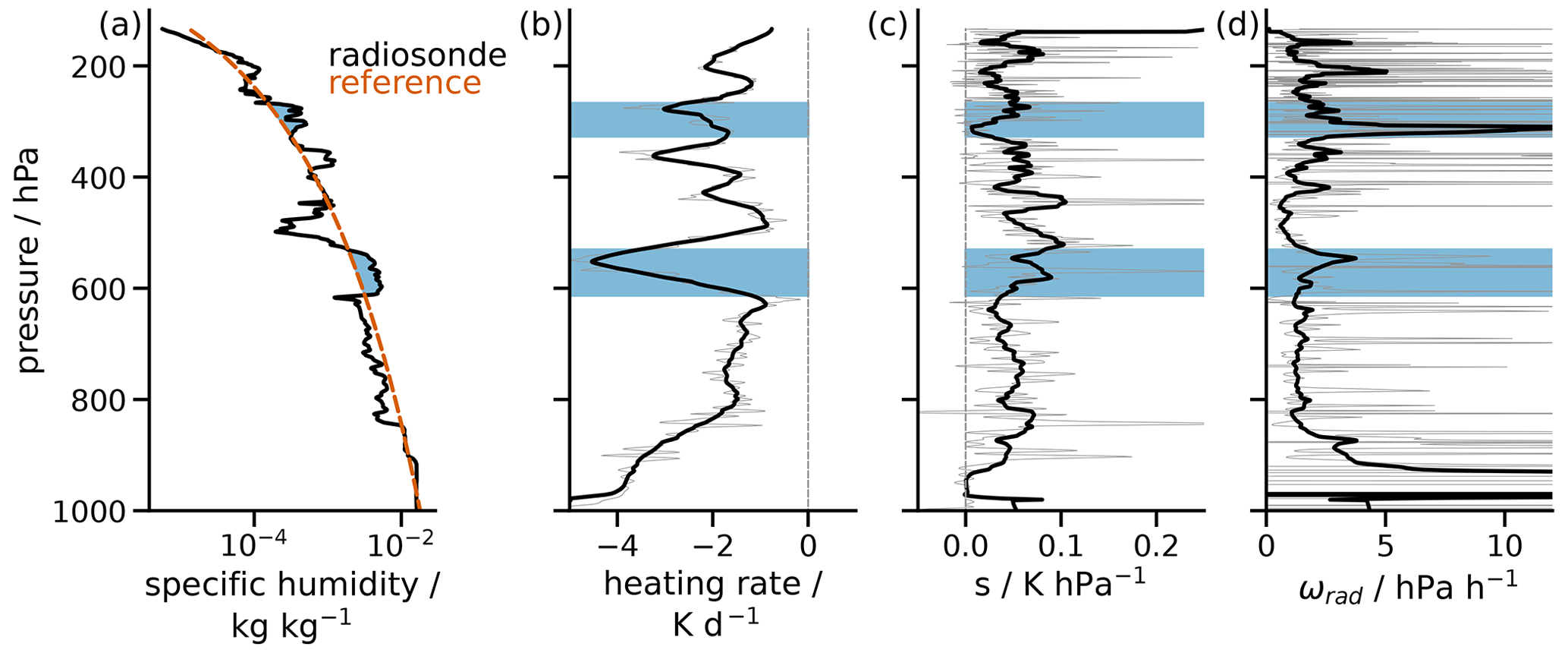
Figure 3GRUAN sounding from 15 February 2012 at 12:00 UTC of (a) H2O volume mixing ratio (VMR), (b) longwave heating rate, (c) static stability and (d) radiatively driven vertical velocity. The dashed red line in panel (a) is the reference humidity profile against which moisture anomalies are identified, which are highlighted by blue shaded regions. Thin grey lines in panels (b), (c) and (d) indicate raw data and thick lines 500 m moving averages.
To assess vertical humidity structures in different datasets, comparing their mean profiles only gives limited information. Positive and negative anomalies can average out, and sharp gradients are smoothed. Hence, we assess the representation of elevated moist layers (EMLs) by identifying them in each dataset and characterising them on a case-by-case basis. We do so through metrics that describe the moist layer strength, vertical thickness and height. Quantifying these properties of vertical moisture structures in the different datasets before applying averaging operators yields more targeted information about vertical moisture variability than averaging directly.
Figure 3a shows an example of a radiosonde humidity profile and the identified moisture anomalies marked by the blue shading. The anomalies are identified and characterised through the method introduced by Prange et al. (2021). The method relies on fitting a second-order polynomial reference profile (dashed red line) against the logarithmic H2O VMR and identifying layers of positive moisture anomaly. These moisture anomalies are characterised by their thickness, height and strength, defined as the vertical integral over the anomalous H2O VMR divided by the layer thickness. The formal definitions of these moisture anomaly characteristics are given by Prange et al. (2021). We only consider moisture anomalies that do not intersect with the 900 and 100 hPa levels and that have a minimum pressure thickness of 50 hPa. This way we constrain our analysis to the free troposphere and make the method less susceptible to small-scale variations that are particularly present in the radiosonde data. Our method identifies two moist layers in the example humidity profile depicted in Fig. 3a (blue shading).
Besides the moisture characteristics described above, we also link the moist layers to their impact on the radiative heating rate (Fig. 3b), where local maxima in cooling are found at the positions of the moist layers. We calculate longwave radiative heating rates with the radiative transfer model RRTMG (Rapid Radiative Transfer Model for GCMs, Mlawer et al., 1997) through its implementation in the radiative convective equilibrium model konrad (Kluft and Dacie, 2020). The strong cooling of the moist layers can be translated into locally increased subsidence rates, which we quantify through the radiatively driven vertical velocity
where s is the static stability defined in Eq. (1). Since s stands in the denominator of ωrad and fluctuates strongly on small vertical scales about values near zero, ωrad also fluctuates strongly. To distill out the radiatively driven dynamical effects in Fig. 3 on the vertical scale of the moist layers, we apply an evenly weighted 500 m moving average to s and Q and calculate ωrad based on the smoothed profiles. This way, local maxima are clearly visible in ωrad in the identified moist layers. It is also apparent that the static stability within the moist layer is a key contributing factor for the magnitude of subsidence. Although the upper-tropospheric moist layer is associated with weaker radiative cooling than the mid-tropospheric one, the lower stability in the upper-tropospheric moist layer results in a stronger subsidence rate.
By calculating moist-layer-associated heating rates, static stabilities and ωrad, we estimate the dynamical effect of moist layers in the different datasets and characterise possible differences in Sect. 6.
We compare the distributions of moisture anomaly characteristics for the four collocation pairs. To start off, the comparison is based on all-sky scenes. In a next step, we distinguish clear-sky from cloudy cases to assess whether cloudiness affects the datasets' capability of capturing moisture anomalies. This is of particular interest for the satellite retrieval datasets, which employ different cloud handling schemes as described in Sect. 2.
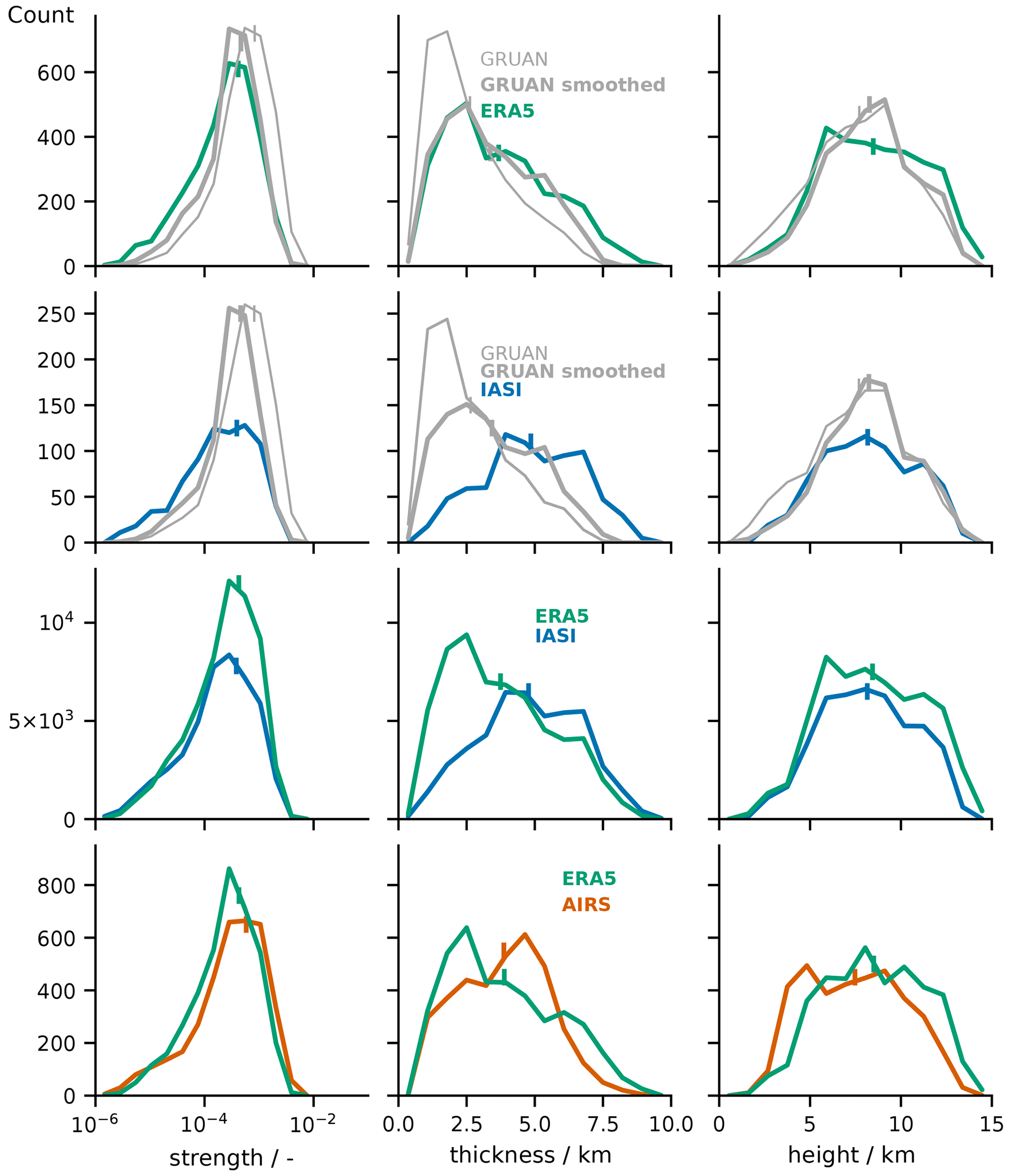
Figure 4Distributions of moist layer characteristics (columns) for the four collocation datasets (rows). Moist layer characteristics are defined by Prange et al. (2021). The thin grey lines refer GRUAN profiles on 10 m vertical resolution, while the thick grey lines represent GRUAN profiles with an applied running mean with a 1 km evenly weighed vertical window.
5.1 All sky
The moisture anomaly identification and characterisation method introduced in Sect. 4 is applied to the humidity profiles of the four collocation datasets. Figure 4 shows the resulting distributions of moisture anomaly characteristics for the four collocation pairs. In the following, we discuss what these results tell us about the different datasets' ability to capture EMLs. We start off with ERA5, then go to IASI and finally to AIRS.
As a first indicator of a dataset's ability to capture moisture anomalies, we compare the number of detected moisture anomalies to the reference dataset, i.e. the areas under the distributions depicted in Fig. 4. ERA5 captures about 99 % as many anomalies as collocated GRUAN data, indicating a good amount of vertical water vapour variability in ERA5 (Fig. 4, first row). Moisture anomalies in ERA5 are about 50 % weaker and 28 % thicker than moisture anomalies in the collocated GRUAN dataset. Moist layers that are less than 2 km in thickness are particularly underrepresented by ERA5, while moist layers with thickness >3 km occur more often. These biases suggest that ERA5 is subject to some degree of smoothing due to limited vertical resolution, which we quantify in the following.
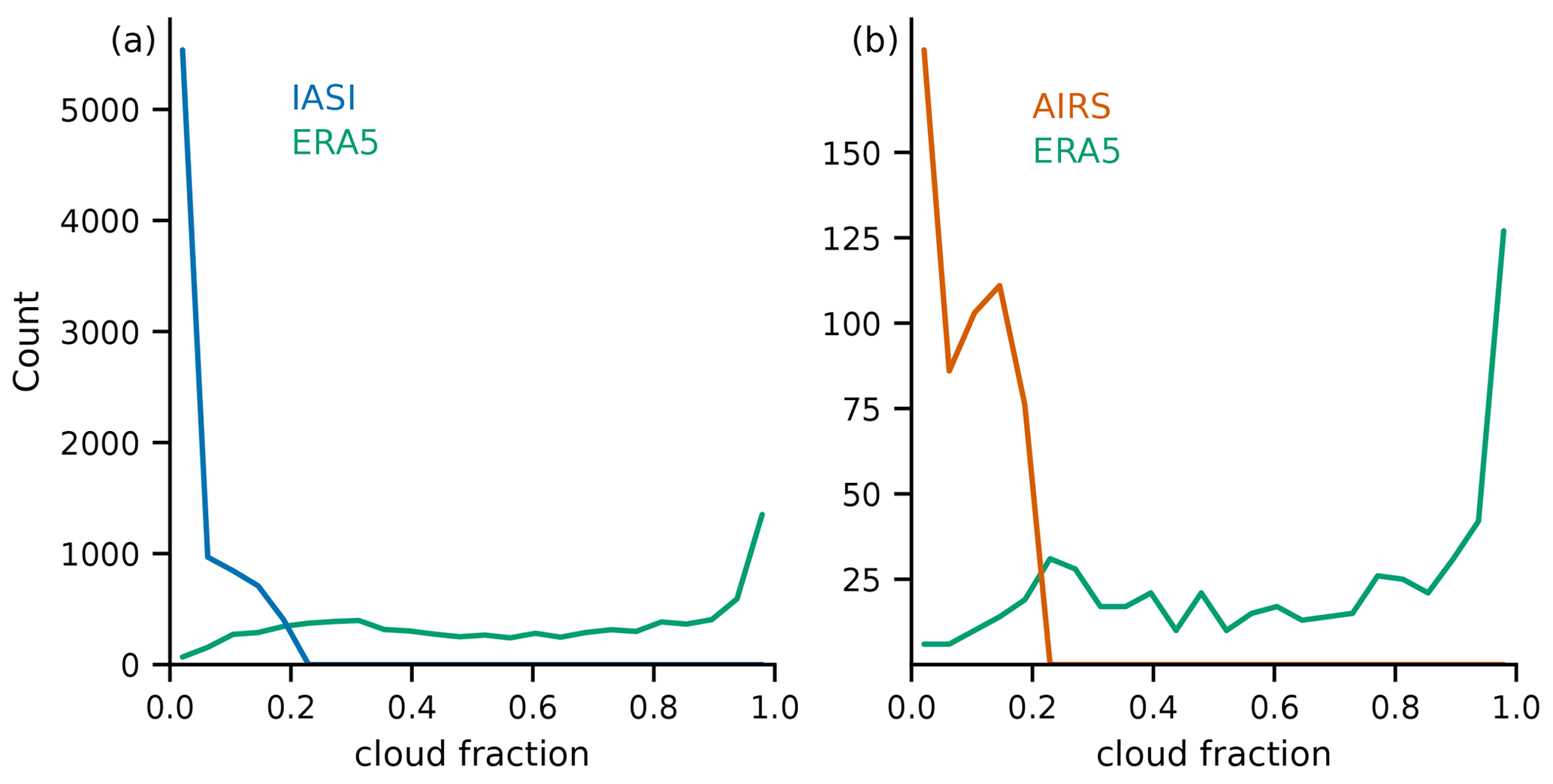
Figure 5Cloud fraction distributions of the two collocation datasets (a) IASI/ERA5 and (b) AIRS/ERA5 after applying a cloud fraction threshold of 0.2 based on the IASI and AIRS cloud fraction estimates.
To investigate to what extent smoothing alone can explain the biases between the moisture anomaly characteristics of ERA5 and GRUAN, we apply a running mean with vertical window size of 1 km and constant weighting to the GRUAN profiles. The resulting distributions are shown as thick lines in the first row of Fig. 4. They show that biases in all three moisture anomaly characteristics can mostly be eliminated through the artificial smoothing. This indicates an effective vertical resolution of the ERA5 humidity profiles in the free troposphere of about 1 km. We conclude that ERA5 captures vertical humidity structures on scales of 1 km and greater well as no systematic deviations from the GRUAN distributions are apparent. Hence, we argue that ERA5 is a suitable reference for assessing the satellite retrieval datasets.
We assess the IASI L2 CDR by comparing it to GRUAN data (Fig. 4, row 2) and ERA5 data (Fig. 4, row 3). The IASI L2 CDR captures about 75 % as many moisture anomalies as in collocated GRUAN data and about 79 % as many moisture anomalies as in collocated ERA5 data. This is a first indicator that the IASI L2 CDR captures less vertical water vapour variability than ERA5. In addition, the maximum in moisture anomaly thickness at around 2 km altitude detected in both GRUAN and ERA5 data is missing in the IASI L2 CDR. Instead, the anomaly thickness distribution is shifted towards significantly higher values with differences in the means of 85 % against GRUAN and 28 % against ERA5. Moisture anomalies are also significantly weaker in the IASI L2 CDR, with mean differences of 53 % and 10 % against GRUAN and ERA5 data, respectively. At this point we want to highlight the added value of assessing the vertical moisture structures of a dataset through moisture characteristics opposed to just comparing the mean profiles (Fig. 2). While we find a strikingly good agreement of the IASI, ERA5 and GRUAN humidity profiles on the mean, quite significant biases become apparent when applying the moist layer characterisation method and then taking a statistical look at how the resulting metrics compare.
As for ERA5, we investigate whether the found biases in anomaly strength and thickness against GRUAN can be explained by smoothing. We apply a 1 km moving average to the GRUAN profiles collocated with the IASI L2 CDR and obtain the moisture anomaly distributions represented by the thick lines (Fig. 4, row 2). While the biases in anomaly strength and height against the IASI dataset are significantly reduced, a strong bias remains in the anomaly thickness. We also attempted to adapt the smoothing window width to different values between 1 and 5 km but do not find the anomaly thickness distribution to approach the one of the IASI dataset much more (not shown). Hence, the bias in anomaly thickness originates from some other source of error in the IASI dataset than smoothing. We come back to this in the next subsection when concentrating on the clear sky.
To assess the AIRS CLIMCAPS retrieval, we rely only on ERA5 as a reference as outlined in Sect. 2.5. The AIRS CLIMCAPS retrieval captures about 92 % as many moisture anomalies as collocated ERA5 data, which is significantly more than the IASI L2 CDR. Moisture anomalies in the AIRS CLIMCAPS retrieval are on average 26 % stronger and 5 % less thick than those in collocated ERA5 data. Also, moist layers in the AIRS CLIMCAPS retrieval are typically found significantly lower in the troposphere compared to the three other datasets; in particular, there are many more moist layer cases below 5 km compared to ERA5. The mean moist layer height is about 1.3 km lower in the AIRS CLIMCAPS retrieval compared to ERA5. We already saw this bias in terms of a shift of the mid-tropospheric humidity peak towards lower altitudes when comparing the dataset mean profiles in Fig. 2. Moisture anomaly strength is a somewhat height-dependent quantity with generally stronger anomalies in the lower troposphere than further up (Prange et al., 2021). Hence, the increased strength of moist layers in the AIRS CLIMCAPS retrieval is to some degree also caused by a bias in moisture anomaly height. Nonetheless, the number of moisture anomalies in the AIRS CLIMCAPS retrieval speaks towards a good capability of the dataset to capture vertical moisture variability – more so than the IASI L2 CDR.
These findings are coherent with the notion of previous case studies that optimal-estimation-based retrievals are more capable of capturing vertical moisture structures than regression-based retrievals (Smith et al., 2012; Weisz et al., 2013; Smith and Weisz, 2018; Zhou et al., 2009; Calbet et al., 2006; Chazette et al., 2014; Prange et al., 2021). A plausible explanation for the superiority of the optimal-estimation-based AIRS CLIMCAPS retrieval is that capturing EMLs is not sufficiently emphasised in the training of the regression-based IASI retrieval. The AIRS CLIMCAPS retrieval is constrained by a priori assumptions about mean and variability of the atmospheric state, but if the optimal estimation setup is tweaked well, deviations from the mean state can be captured well with this method.

5.2 Clear sky
The satellite retrieval products do operate in the presence of clouds, but information content is limited with increased cloudiness and cloud depth, in particular from the infrared instruments. Hence, we are interested in whether our analysis of moisture anomaly characteristics yields different results when limited to clear-sky scenes compared to the previously investigated all-sky scenes. Possible differences could then potentially be linked to the different cloud handling schemes deployed by the retrieval products (Sect. 2).
The AIRS CLIMCAPS and IASI L2 retrievals come with an estimate of total cloud fraction for each retrieval pixel, which are obtained based on quite different methods as outlined in Sect. 2. ERA5 also provides a total cloud fraction variable, which we show in addition but do not base our further analysis on since it appears quite biased against the satellite-derived cloud fractions. As suggested in the CLIMCAPS science application guide, we use a cloud fraction threshold of 0.2 to distinguish clear-sky from cloudy scenes (Smith et al., 2021). For the two collocation datasets IASI/ERA5 and AIRS/ERA5, this leaves about 22 % of the all-sky amount of data. For the IASI/GRUAN comparison, sampling becomes too limited, which is why we limit this analysis to the satellite collocations with ERA5.
Figure 5 shows the resulting cloud fraction distributions of the two collocation datasets. It is striking that when limiting satellite-based cloud fractions to 0.2, ERA5 cloud fraction estimates show maxima near cloud fractions of 1. Without any applied thresholds, both satellite datasets also have their global maxima near cloud fractions of 1 (not shown). However, the secondary maximum near 0 found in both satellite datasets is not at all present in ERA5. Compared to CLIMCAPS, we would have expected a stronger bimodality between high and low cloud fractions in ERA5 due to the higher spatial resolution of ERA5 of 31 km compared to about 50 km in the nadir view of the CLIMCAPS product. However, since cloud fraction requires subgrid-scale knowledge, it is difficult to define this variable in a model framework. Hence, finding significant differences to satellite-derived estimates is not completely surprising.
Figure 6 shows the resulting moisture anomaly characteristics after application of the clear-sky filter. All datasets consistently show an increase in mean anomaly strength of about 20 % compared to the all-sky results. Note that our method for quantifying anomaly strength is designed to capture the magnitude of vertical moisture variability rather than absolute amount of humidity, which would be highest in the event of clouds (Prange et al., 2021). The found increase in anomaly strength in the clear sky is in line with our expectations because in cloudy conditions vertical humidity variability is limited by the saturation humidity, leading to weaker moisture anomalies.
We also see a significant change in the shape of the anomaly height distributions when comparing clear sky to all sky. IASI and ERA5 both show a clear bimodal structure in anomaly height in the clear sky, which was not the case in the all-sky data. Physically, we explain the position of the maxima near 5 and 12 km by levels of preferred detrainment of moist air from mid-level or deep convective plumes into the clear-sky environment (Johnson et al., 1999; Romps, 2014). The mid-level detrainment is thought to be driven by enhanced stability near the melting level, and the upper-tropospheric detrainment is associated with increased stability towards the tropopause as the atmosphere goes into pure radiative equilibrium aloft. We hypothesise that the mid-tropospheric peak is more pronounced than the upper-tropospheric peak in ERA5 and IASI anomaly height distributions because both deep (cumulonimbus) and mid-level (cumulus congestus) convection causes mid-level detrainment, while only deep convection causes upper level detrainment. AIRS also shows peaks in anomaly height near 5 and 12 km and another peak in between at around 7 km that we can not link to a physical mechanism in this height. However, when interpreting the detailed shape of the distributions to this extent, we advice caution due to the limited number of AIRS/ERA5 collocations, which is only about 10 % of the number of IASI/ERA5 collocations.
We do not find significant changes in biases between satellite retrievals and ERA5 in anomaly strength or thickness when limiting our data to clear sky. While we do see changes in the means of the distributions as described above, biases remain similar. Although biases do not change much, we see that the all-sky secondary maximum at large anomaly thickness values of IASI, which is not present in ERA5 (Fig. 4), vanishes in the clear sky, indicating better vertical resolution. However, going to clear sky does not reduce the gap between satellite retrievals and ERA5 at anomaly thickness values below 3 km. We conclude that the retrievals' observing capability of moist layers is not significantly limited by clouds.
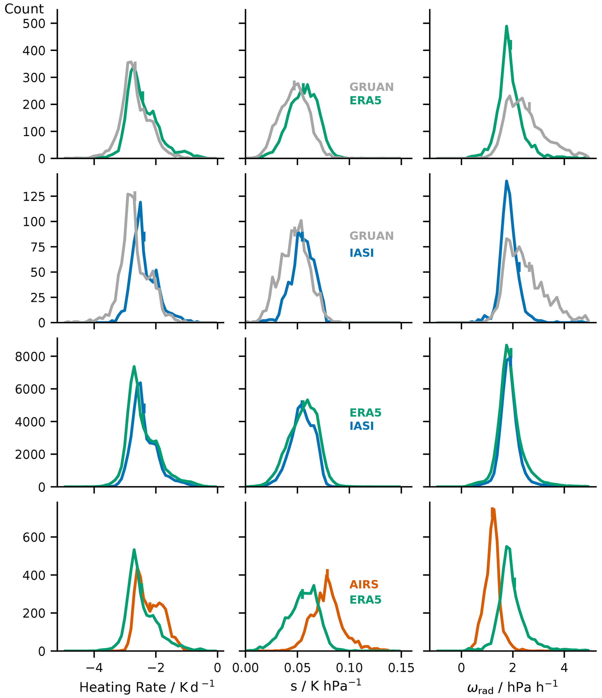
Figure 7Distributions of moist-layer-associated longwave heating rate, static stability (s) and radiatively driven vertical velocity ωrad for the different collocation datasets. The averaging measure for heating rate is the median. s is calculated based on moist layer median temperature, potential temperature and potential temperature gradient. ωrad is calculated by division of moist-layer-associated heating rate and static stability. Vertical dashes indicate means.
In this section we want to translate the datasets' varying capabilities to resolve EMLs found in Sect. 5.1 into estimates of the moist layers' effect on meso-scale dynamics. EMLs are thought to impact the meso-scale dynamics of the atmosphere through their effect on the spatial structure of radiative heating (Stevens et al., 2017). We attempt to draw a direct connection between EMLs and dynamics by translating their effect on the heating rates into radiatively driven vertical velocities ωrad, for which to a first order the static stability is another contributing factor (Sect. 4).
Figure 7 shows distributions of moist-layer-associated longwave heating rates, static stabilities (s) and radiatively driven vertical velocities (Eq. 2). The same moist layers identified as basis for Fig. 4 are used here, and the three additional quantities are calculated for each moist layer. This is done by calculating the vertical median heating rate across each identified moist layer (Fig. 7, column 1). To calculate the moist layer averaged static stability s according to Eq. (1), moist layer median temperatures, potential temperatures and potential temperature gradients are used (Fig. 7, column 2). The resulting moist-layer-associated heating rates and static stabilities are used to calculate the moist-layer-associated ωrad (Fig. 7, column 3).
The typical tropical free-tropospheric heating rate is on the order of −2 K d−1 (Jeevanjee and Fueglistaler, 2020). Moist-layer-associated heating rates depicted in the first column of Fig. 7 show their peak at more negative values of around −3 K d−1 because of the locally enhanced infrared opacity of the moist layers that cause increased infrared absorption and cooling to space. However, a saddle point in the distributions is found at −2 K d−1, which is associated with particularly weak moisture anomalies that barely increase opacity. The fact that most heating rates are found at values lower than −2 K d−1 shows that our method does in fact filter for the moisture features we are interested in.
We expect biases in moist-layer-associated heating rates between the collocated datasets to reflect biases in moist layer strength and thickness; i.e. stronger and thinner moist layers go along with more pronounced cooling. We find this to generally be the case as GRUAN shows the strongest moist-layer-associated cooling, followed by only a slight bias to ERA5 and slightly more cooling in the IASI L2 retrieval than in the AIRS CLIMCAPS retrieval. Differences in heating rate distributions between ERA5 and GRUAN are small, indicating that the found biases in moisture anomaly strength and thickness that could mostly be eliminated by applying 1 km vertical smoothing to the radiosonde data are not very significant for the moist-layer-associated heating rates. However, we also find a 19 % difference in the means of static stability between ERA5 and GRUAN that adds to the slightly enhanced cooling in GRUAN to result in a 38 % difference in ωrad means between the two datasets. Static stability values also showed to be increased in ERA5 compared to GRUAN in the comparison of the 4-year mean profiles in Fig. 2.
For the IASI/GRUAN comparison, similar biases are found as for ERA5. The ERA5/IASI comparison reveals that slightly stronger cooling rates found in ERA5 are balanced by slightly increased static stabilities in ERA5 yielding only a 0.7 % difference in ωrad means between ERA5 and IASI.
Stronger biases are found between ERA5 and AIRS. Moist-layer-associated cooling is weakest in the AIRS dataset among all investigated datasets. In addition, AIRS shows significantly enhanced stability with a 44 % mean difference against ERA5, while ERA5 already showed enhanced stability compared to GRUAN. The moist-layer-associated weaker cooling and enhanced stability in AIRS yield a 43 % mean difference in ωrad against ERA5 and an about 80 % mean difference to the GRUAN mean ωrad obtained from collocations with ERA5 and IASI.
To put the found values of ωrad and associated biases between the datasets into some perspective, we compare our results to measurements of meso-scale vertical pressure velocities ω obtained from dropsonde measurements of the EUREC4A field campaign. During EUREC4A, the HALO aircraft flew 69 circles of about 200 km diameter, launching 12 dropsondes per circle (Konow et al., 2021; George et al., 2021). Using the method of Bony and Stevens (2019), circle-integrated profiles of divergence allow for a deduction of ω, some first EUREC4A averaged results of which are presented by Stevens et al. (2021). The campaign mean ranges between values of 1 and 2 hPa h−1 throughout the free troposphere, while individual circles show maximum variations between −5 and 10 hPa h−1. The moist-layer-associated ωrad values we find based on GRUAN with values between 1.5 and 4 hPa h−1 are generally higher than the mean meso-scale ω measurements. We conclude that EMLs show a significant radiative impact on meso-scale dynamics when compared to meso-scale measurements of ω. With biases of moist-layer-associated ωrad in ERA5, IASI and AIRS data ranging from 38 % to 80 % compared to GRUAN and ωrad means being on a similar order as meso-scale ω measurements, we conclude that these datasets have limited usability to assess the dynamical impact of EMLs.
We assessed ERA5 reanalysis data, the IASI Level 2 Climate Data Record (CDR) and the CLIMCAPS-Aqua Level 2 retrieval product in terms of their ability to capture vertical moisture structures, in particular EMLs. As reference, we use 2146 radiosonde soundings from Manus Island of the years 2011 to 2014 that are part of the quality-controlled GRUAN network. We compared mean profiles of temperature, humidity, and static stability and then identified and characterised collocated moist layers using the method of Prange et al. (2021) as basis and assessed the moist layers' impact on the dynamics in terms of radiative heating and radiatively driven vertical velocities. In the following, we draw conclusions about our main question – that is, how adequately are EMLs represented in the different data products?
-
The 4-year mean profiles show a clear mid-tropospheric maximum in relative humidity in all data products that is associated with EMLs. It is similarly pronounced in ERA5, IASI and GRUAN. Only the AIRS CLIMCAPS retrieval shows significant humidity biases against the other data products. The mid-tropospheric humidity peak is not located near the melting level as in the other datasets but about 100 hPa lower, causing a significant moist bias in the lower to middle free troposphere. A peak in mid-tropospheric static stability is also located about 100 hPa lower than in ERA5. In the upper troposphere between about 400 and 100 hPa the AIRS CLIMCAPS retrieval shows a dry bias against the other datasets.
-
The number of identified moist layers based on the method described in Sect. 4 is almost equal between collocated ERA5 and GRUAN data, indicating a good amount of vertical water vapour variability in ERA5. Moist layers in ERA5 are about 50 % weaker and 28 % thicker than moist layers in GRUAN data. These biases can be completely negated by applying a 1 km moving average to GRUAN profiles, indicating 1 km effective vertical resolution of ERA5 humidity profiles. The AIRS retrieval shows about 92 % as many moist layers as ERA5 and the IASI retrieval only about 79 %, indicating slightly enhanced vertical moisture variability in the AIRS retrieval compared to IASI. In addition, the IASI retrieval shows about 53 % weaker and 85 % thicker moist layers than collocated GRUAN data. We find that these biases in IASI can not completely be negated by applying vertical smoothing to the GRUAN data, indicating other sources of error than pure smoothing. The AIRS retrieval shows moist layers that are stronger than and similarly as thick as ERA5. However, moist layers are generally found about 1.3 km lower in the troposphere than in ERA5, which limits the conclusiveness of comparing moist layer strength, since moist layers further down are typically stronger.
-
Reducing the investigated collocated scenes between the two retrieval datasets and ERA5 to clear sky is found to not significantly change biases in moist layer strength and thickness, indicating that the cloud handling schemes are not the limiting factors for the retrievals' ability to resolve moist layers. While distributions of total cloud fractions are comparable between the two retrieval datasets, collocated ERA5 total cloud fractions show strong deviations towards cloud fractions of 1, while retrieval cloud fractions are limited to less than 0.2. These biases merit further study.
-
Moist-layer-associated heating rates are on average on the order of −3 K d−1, showing enhanced cooling compared to the mean tropical free-tropospheric cooling of about −2 K d−1 (Jeevanjee and Fueglistaler, 2020). Slight biases in moist-layer-associated heating rates are found between the datasets that are representative of the found biases in moist layer strength, thickness and height. Consequently, we find the strongest moist-layer-associated cooling in GRUAN data and the weakest cooling in the AIRS CLIMCAPS retrieval, which we attribute to its significant bias towards lower moist layer heights where cooling to space is less effective due to the bigger column of water vapour above the moist layers.
-
We find that, on average, the moist-layer-associated radiatively driven subsidence ωrad at 1.5 to 4 hPa h−1 is higher than mean meso-scale subsidence deduced from EUREC4A field campaign measurements at about 1 to 2 hPa h−1 (Stevens et al., 2021). Hence, EMLs are relevant for meso-scale atmospheric dynamics. According to Eq. (2), ωrad is controlled by both moist-layer-associated radiative cooling and static stability. Biases between datasets in both of those quantities are significant for the resulting biases in ωrad, which is 38 % for both ERA5 and IASI with respect to GRUAN and 43 % for the AIRS CLIMCAPS retrieval with respect to ERA5. We conclude that due to these significant relative biases, all datasets have limited usefulness to assess the dynamical impact of EMLs.
Given the inherently limited vertical resolution of reanalysis and retrieval products compared to in situ soundings, we find ERA5 to resolve EMLs well, while IASI and AIRS show some more significant biases that can not be explained purely by vertical smoothing. The IASI L2 CDR shows most significant biases in moist layer thickness that may be possible to improve by more strongly emphasising EMLs in the retrieval's training or by introducing an optimal estimation step to the retrieval as for example found by Calbet et al. (2006), the downside of which would be the computational cost. Since an optimal estimation step is already included in the near-real-time production of IASI L2 retrievals (EUMETSAT, 2017), our results based on CLIMCAPS suggest that it may be worth considering including the optimal estimation step also in the production of the IASI L2 CDR.
We find the AIRS CLIMCAPS retrieval to be subject to significant humidity biases, in particular with respect to moist layer height. Studying the origins of these biases remains a future task, but we see no inherent reason why it would not be possible to eliminate them. In this context, we would encourage investigating the reanalysis product MERRA-2, which is used as prior knowledge for the CLIMCAPS retrieval product, to see whether biases in CLIMCAPS are to some degree inherited from MERRA-2.
The code used to calculate the radiative heating rates has been made publicly available by Kluft and Dacie (2020) (https://doi.org/10.5281/zenodo.3899702). The code to collocate datasets is available as part of the Python package typhon (Lemke et al., 2021; https://doi.org/10.5281/zenodo.5786028).
The collocation datasets are publicly available on Zenodo (Prange et al., 2022). These include only the data that are used to deduce our results, i.e. after quality control criteria and processing steps as described in Sect. 2 have been applied.
MP conducted the data analysis and prepared the manuscript. SAB and MB supervised the data analysis, contributed ideas to the manuscript and revised it.
The authors declare that they have no conflict of interest.
Publisher’s note: Copernicus Publications remains neutral with regard to jurisdictional claims in published maps and institutional affiliations.
This article is part of the special issue “Analysis of atmospheric water vapour observations and their uncertainties for climate applications (ACP/AMT/ESSD/HESS inter-journal SI)”. It is not associated with a conference.
The authors would like to thank the GRUAN community and the Atmospheric Radiation Measurement programme for making the sounding data from Manus Island freely available. The authors would like to thank EUMETSAT for their support in making the analysed IASI L2 CDR available to us. The authors would like to thank the AIRS community for making the analysed CLIMCAPS-Aqua Level 2 dataset freely available for download and providing helpful documentation in their science application guide.
This work contributes to the Cluster of Excellence Climate, Climatic Change, and Society (CLICCS) and to the Center for Earth System Research and Sustainability (CEN) of Universität Hamburg.
This work was funded by the German Research Foundation (DFG) in the project “Elevated Moist Layers – Using HALO during EUREC4A to explore a blind spot in the global satellite observing system”, project BU 2253/9-1, part of DFG priority programme HALO SPP 1294, project number 316646266.
This paper was edited by Farahnaz Khosrawi and reviewed by Nadia Smith and one anonymous referee.
Ackerman, T. P. and Stokes, G. M.: The Atmospheric Radiation Measurement Program, Phys. Today, 56, 38–44, https://doi.org/10.1063/1.1554135, 2003. a
Berndt, E., Smith, N., Burks, J., White, K., Esmaili, R., Kuciauskas, A., Duran, E., Allen, R., LaFontaine, F., and Szkodzinski, J.: Gridded Satellite Sounding Retrievals in Operational Weather Forecasting: Product Description and Emerging Applications, Remote Sens., 12, 3311, https://doi.org/10.3390/rs12203311, 2020. a
Bony, S. and Stevens, B.: Measuring Area-Averaged Vertical Motions with Dropsondes, J. Atmos. Sci., 76, 767–783, https://doi.org/10.1175/JAS-D-18-0141.1, 2019. a
Bony, S., Stevens, B., Frierson, D. M. W., Jakob, C., Kageyama, M., Pincus, R., Shepherd, T. G., Sherwood, S. C., Siebesma, A. P., Sobel, A. H., Watanabe, M., and Webb, M. J.: Clouds, circulation and climate sensitivity, Nat. Geosci., 8, 261–268, https://doi.org/10.1038/ngeo2398, 2015. a
Brands, S., Herrera, S., Fernández, J., and Gutiérrez, J. M.: How well do CMIP5 Earth System Models simulate present climate conditions in Europe and Africa?, Clim. Dynam., 41, 803–817, https://doi.org/10.1007/s00382-013-1742-8, 2013. a
Buehler, S. A., Östman, S., Melsheimer, C., Holl, G., Eliasson, S., John, V. O., Blumenstock, T., Hase, F., Elgered, G., Raffalski, U., Nasuno, T., Satoh, M., Milz, M., and Mendrok, J.: A multi-instrument comparison of integrated water vapour measurements at a high latitude site, Atmos. Chem. Phys., 12, 10925–10943, https://doi.org/10.5194/acp-12-10925-2012, 2012. a
Calbet, X., Schlüssel, P., Hultberg, T., Phillips, P., and August, T.: Validation of the operational IASI level 2 processor using AIRS and ECMWF data, Adv. Space Res., 37, 2299–2305, https://doi.org/10.1016/j.asr.2005.07.057, 2006. a, b
Cardinali, C.: Monitoring the observation impact on the short-range forecast, Q. J. Roy. Meteorol. Soc., 135, 239–250, https://doi.org/10.1002/qj.366, 2009. a
Chazette, P., Marnas, F., Totems, J., and Shang, X.: Comparison of IASI water vapor retrieval with H2O-Raman lidar in the framework of the Mediterranean HyMeX and ChArMEx programs, Atmos. Chem. Phys., 14, 9583–9596, https://doi.org/10.5194/acp-14-9583-2014, 2014. a
Dahoui, M., Isaksen, L., and Radnoti, G.: Assessing the impact of observations using observation-minus-forecast residuals, ECMWF Newsletter, 152, 27–31, https://doi.org/10.21957/51j3sa, 2017. a
Dirksen, R. J., Sommer, M., Immler, F. J., Hurst, D. F., Kivi, R., and Vömel, H.: Reference quality upper-air measurements: GRUAN data processing for the Vaisala RS92 radiosonde, Atmos. Meas. Tech., 7, 4463–4490, https://doi.org/10.5194/amt-7-4463-2014, 2014. a, b
ECMWF: IFS Documentation CY41R2 – Part III: Dynamics and Numerical Procedures, 3, https://doi.org/10.21957/83wouv80, 2016. a
ECMWF: IFS Documentation – Cy45r1, Chap. Part IV: Physical processes, p. 203, ECMWF, https://www.ecmwf.int/en/elibrary/80895-ifs-documentation-cy45r1-part-iv-physical-processes (last access: 3 January 2023), 2018. a
EUMETSAT: IASI Level 2: Product Guide, EUMETSAT, https://www.eumetsat.int/media/45982 (last access: 3 January 2023), 2017. a, b, c
EUMETSAT: IASI All Sky Temperature and Humidity Profiles – Climate Data Record Release 1.1 – Metop-A and -B, https://doi.org/10.15770/EUM_SEC_CLM_0063, 2022. a, b, c
Eyring, V., Bony, S., Meehl, G. A., Senior, C. A., Stevens, B., Stouffer, R. J., and Taylor, K. E.: Overview of the Coupled Model Intercomparison Project Phase 6 (CMIP6) experimental design and organization, Geosci. Model Dev., 9, 1937–1958, https://doi.org/10.5194/gmd-9-1937-2016, 2016. a
Ferraro, R., Waliser, D. E., Gleckler, P., Taylor, K. E., and Eyring, V.: Evolving Obs4MIPs to Support Phase 6 of the Coupled Model Intercomparison Project (CMIP6), B. Am. Meteorol. Soc., 96, ES131–ES133, https://doi.org/10.1175/BAMS-D-14-00216.1, 2015. a
George, G., Stevens, B., Bony, S., Pincus, R., Fairall, C., Schulz, H., Kölling, T., Kalen, Q. T., Klingebiel, M., Konow, H., Lundry, A., Prange, M., and Radtke, J.: JOANNE: Joint dropsonde Observations of the Atmosphere in tropical North atlaNtic meso-scale Environments, Earth Syst. Sci. Data, 13, 5253–5272, https://doi.org/10.5194/essd-13-5253-2021, 2021. a
Hersbach, H., Bell, B., Berrisford, P., Hirahara, S., Horányi, A., Muñoz-Sabater, J., Nicolas, J., Peubey, C., Radu, R., Schepers, D., Simmons, A., Soci, C., Abdalla, S., Abellan, X., Balsamo, G., Bechtold, P., Biavati, G., Bidlot, J., Bonavita, M., Chiara, G., Dahlgren, P., Dee, D., Diamantakis, M., Dragani, R., Flemming, J., Forbes, R., Fuentes, M., Geer, A., Haimberger, L., Healy, S., Hogan, R. J., Hólm, E., Janisková, M., Keeley, S., Laloyaux, P., Lopez, P., Lupu, C., Radnoti, G., Rosnay, P., Rozum, I., Vamborg, F., Villaume, S., and Thépaut, J.-N.: The ERA5 global reanalysis, Q. J. Roy. Meteorol. Soc., 146, 1999–2049, https://doi.org/10.1002/qj.3803, 2020. a
Jeevanjee, N. and Fueglistaler, S.: Simple Spectral Models for Atmospheric Radiative Cooling, J. Atmos. Sci., 77, 479–497, https://doi.org/10.1175/JAS-D-18-0347.1, 2020. a, b
Jiang, J. H., Su, H., Zhai, C., Perun, V. S., Genio, A. D., Nazarenko, L. S., Donner, L. J., Horowitz, L., Seman, C., Cole, J., Gettelman, A., Ringer, M. A., Rotstayn, L., Jeffrey, S., Wu, T., Brient, F., Dufresne, J.-L., Kawai, H., Koshiro, T., Watanabe, M., LÉcuyer, T. S., Volodin, E. M., Iversen, T., Drange, H., Mesquita, M. D. S., Read, W. G., Waters, J. W., Tian, B., Teixeira, J., and Stephens, G. L.: Evaluation of cloud and water vapor simulations in CMIP5 climate models using NASA “A-Train” satellite observations, J. Geophys. Res.-Atmos., 117, D14105, https://doi.org/10.1029/2011JD017237, 2012. a
Johnson, R. H., Ciesielski, P. E., and Hart, K. A.: Tropical Inversions near the 0 °C Level, J. Atmos. Sci., 53, 1838–1855, https://doi.org/10.1175/1520-0469(1996)053<1838:TINTL>2.0.CO;2, 1996. a, b, c
Johnson, R. H., Rickenbach, T. M., Rutledge, S. A., Ciesielski, P. E., and Schubert, W. H.: Trimodal Characteristics of Tropical Convection, J. Climate, 12, 2397–2418, https://doi.org/10.1175/1520-0442(1999)012<2397:TCOTC>2.0.CO;2, 1999. a, b
Keil, P., Schmidt, H., Stevens, B., and Bao, J.: Variations of Tropical Lapse Rates in Climate Models and their Implications for Upper Tropospheric Warming, J. Climate, 34, 1–50, https://doi.org/10.1175/JCLI-D-21-0196.1, 2021. a, b, c, d
Kluft, L. and Dacie, S.: atmtools/konrad, Zenodo [code], https://doi.org/10.5281/zenodo.3899702, 2020. a, b
Konow, H., Ewald, F., George, G., Jacob, M., Klingebiel, M., Kölling, T., Luebke, A. E., Mieslinger, T., Pörtge, V., Radtke, J., Schäfer, M., Schulz, H., Vogel, R., Wirth, M., Bony, S., Crewell, S., Ehrlich, A., Forster, L., Giez, A., Gödde, F., Groß, S., Gutleben, M., Hagen, M., Hirsch, L., Jansen, F., Lang, T., Mayer, B., Mech, M., Prange, M., Schnitt, S., Vial, J., Walbröl, A., Wendisch, M., Wolf, K., Zinner, T., Zöger, M., Ament, F., and Stevens, B.: EUREC4A's HALO, Earth Syst. Sci. Data, 13, 5545–5563, https://doi.org/10.5194/essd-13-5545-2021, 2021. a
Lang, T., Naumann, A. K., Stevens, B., and Buehler, S. A.: Tropical Free-Tropospheric Humidity Differences and Their Effect on the Clear-Sky Radiation Budget in Global Storm-Resolving Models, J. Adv. Model. Earth Syst., 13, e2021MS002514, https://doi.org/10.1029/2021MS002514, 2021. a, b
Lemke, O., Kluft, L., Mrziglod, J., Pfreundschuh, S., Holl, G., Larsson, R., Yamada, T., Mieslinger, T., and Doerr, J.: atmtools/typhon: Typhon Release 0.9.0 (v0.9.0), Zenodo [code], https://doi.org/10.5281/zenodo.5786028, 2021. a
Mapes, B. E. and Zuidema, P.: Radiative-Dynamical Consequences of Dry Tongues in the Tropical Troposphere, J. Atmos. Sci., 53, 620–638, https://doi.org/10.1175/1520-0469(1996)053<0620:RDCODT>2.0.CO;2, 1996. a
Mlawer, E. J., Taubman, S. J., Brown, P. D., Iacono, M. J., and Clough, S. A.: Radiative transfer for inhomogeneous atmospheres: RRTM, a validated correlated-k model for the longwave, J. Geophys. Res.-Atmos., 102, 16663–16682, https://doi.org/10.1029/97JD00237, 1997. a
Muller, C. and Bony, S.: What favors convective aggregation and why?, Geophys. Res. Lett., 42, 5626–5634, https://doi.org/10.1002/2015GL064260, 2015. a
Muller, C., Yang, D., Craig, G., Cronin, T., Fildier, B., Haerter, J. O., Hohenegger, C., Mapes, B., Randall, D., Shamekh, S., and Sherwood, S. C.: Spontaneous Aggregation of Convective Storms, Ann. Rev. Fluid Mechan., 54, 133–157, https://doi.org/10.1146/annurev-fluid-022421-011319, 2022. a
Posselt, D. J., van den Heever, S. C., and Stephens, G. L.: Trimodal cloudiness and tropical stable layers in simulations of radiative convective equilibrium, Geophys. Res. Lett., 35, L08802, https://doi.org/10.1029/2007GL033029, 2008. a
Prange, M., Brath, M., and Buehler, S. A.: Are elevated moist layers a blind spot for hyperspectral infrared sounders? A model study, Atmos. Meas. Tech., 14, 7025–7044, https://doi.org/10.5194/amt-14-7025-2021, 2021. a, b, c, d, e, f, g, h, i
Prange, M., Buehler, S. A., and Brath, M.: Supplementary data for “How adequately are elevated moist layers represented in reanalysis and satellite observations?”, Zenodo [data set], https://doi.org/10.5281/zenodo.6940500, 2022. a
Rodgers, C. D.: Inverse Methods for Atmospheric Sounding, Ocean. Planet. Phys., Vol. 2, World Scientific, https://doi.org/10.1142/3171, 2000. a
Romps, D. M.: An Analytical Model for Tropical Relative Humidity, J. Climate, 27, 7432–7449, https://doi.org/10.1175/JCLI-D-14-00255.1, 2014. a, b, c
Schulz, H. and Stevens, B.: Observing the Tropical Atmosphere in Moisture Space, J. Atmos. Sci., 75, 3313–3330, https://doi.org/10.1175/JAS-D-17-0375.1, 2018. a
Seidel, D. J., Berger, F. H., Diamond, H. J., Dykema, J., Goodrich, D., Immler, F., Murray, W., Peterson, T., Sisterson, D., Sommer, M., Thorne, P., Vomel, H., and Wang, J.: Reference Upper-Air Observations for Climate: Rationale, Progress, and Plans, B. Am. Meteorol. Soc., 90, 361–369, https://doi.org/10.1175/2008BAMS2540.1, 2009. a
Smith, N. and Barnet, C. D.: Uncertainty Characterization and Propagation in the Community Long-Term Infrared Microwave Combined Atmospheric Product System (CLIMCAPS), Remote Sens., 11, 1227, https://doi.org/10.3390/rs11101227, 2019. a
Smith, N. and Barnet, C. D.: CLIMCAPS observing capability for temperature, moisture, and trace gases from AIRS/AMSU and CrIS/ATMS, Atmos. Meas. Tech., 13, 4437–4459, https://doi.org/10.5194/amt-13-4437-2020, 2020. a, b
Smith, N., Esmaili, R., and Barnet, C. D.: Community Long-term Infrared Microwave CombinedAtmospheric Product System (CLIMCAPS) Science Application Guides, https://docserver.gesdisc.eosdis.nasa.gov/public/project/Sounder/CLIMCAPS_V2_L2_science_guides.pdf (last access: 3 January 2023), 2021. a, b, c
Smith, W. and Weisz, E.: Dual-Regression Approach for High-Spatial-Resolution Infrared Soundings, 297–311 pp., Comprehensive Remote Sensing, Elsevier, https://doi.org/10.1016/B978-0-12-409548-9.10394-X, 2018. a
Smith, W. L., Weisz, E., Kireev, S. V., Zhou, D. K., Li, Z., and Borbas, E. E.: Dual-Regression Retrieval Algorithm for Real-Time Processing of Satellite Ultraspectral Radiances, J. Appl. Meteorol. Climatol., 51, 1455–1476, https://doi.org/10.1175/JAMC-D-11-0173.1, 2012. a
Stevens, B., Brogniez, H., Kiemle, C., Lacour, J.-L., Crevoisier, C., and Kiliani, J.: Structure and Dynamical Influence of Water Vapor in the Lower Tropical Troposphere, Surv. Geophys., 38, 1371–1397, https://doi.org/10.1007/s10712-017-9420-8, 2017. a, b, c, d, e, f
Stevens, B., Bony, S., Farrell, D., Ament, F., Blyth, A., Fairall, C., Karstensen, J., Quinn, P. K., Speich, S., Acquistapace, C., Aemisegger, F., Albright, A. L., Bellenger, H., Bodenschatz, E., Caesar, K.-A., Chewitt-Lucas, R., de Boer, G., Delanoë, J., Denby, L., Ewald, F., Fildier, B., Forde, M., George, G., Gross, S., Hagen, M., Hausold, A., Heywood, K. J., Hirsch, L., Jacob, M., Jansen, F., Kinne, S., Klocke, D., Kölling, T., Konow, H., Lothon, M., Mohr, W., Naumann, A. K., Nuijens, L., Olivier, L., Pincus, R., Pöhlker, M., Reverdin, G., Roberts, G., Schnitt, S., Schulz, H., Siebesma, A. P., Stephan, C. C., Sullivan, P., Touzé-Peiffer, L., Vial, J., Vogel, R., Zuidema, P., Alexander, N., Alves, L., Arixi, S., Asmath, H., Bagheri, G., Baier, K., Bailey, A., Baranowski, D., Baron, A., Barrau, S., Barrett, P. A., Batier, F., Behrendt, A., Bendinger, A., Beucher, F., Bigorre, S., Blades, E., Blossey, P., Bock, O., Böing, S., Bosser, P., Bourras, D., Bouruet-Aubertot, P., Bower, K., Branellec, P., Branger, H., Brennek, M., Brewer, A., Brilouet , P.-E., Brügmann, B., Buehler, S. A., Burke, E., Burton, R., Calmer, R., Canonici, J.-C., Carton, X., Cato Jr., G., Charles, J. A., Chazette, P., Chen, Y., Chilinski, M. T., Choularton, T., Chuang, P., Clarke, S., Coe, H., Cornet, C., Coutris, P., Couvreux, F., Crewell, S., Cronin, T., Cui, Z., Cuypers, Y., Daley, A., Damerell, G. M., Dauhut, T., Deneke, H., Desbios, J.-P., Dörner, S., Donner, S., Douet, V., Drushka, K., Dütsch, M., Ehrlich, A., Emanuel, K., Emmanouilidis, A., Etienne, J.-C., Etienne-Leblanc, S., Faure, G., Feingold, G., Ferrero, L., Fix, A., Flamant, C., Flatau, P. J., Foltz, G. R., Forster, L., Furtuna, I., Gadian, A., Galewsky, J., Gallagher, M., Gallimore, P., Gaston, C., Gentemann, C., Geyskens, N., Giez, A., Gollop, J., Gouirand, I., Gourbeyre, C., de Graaf, D., de Groot, G. E., Grosz, R., Güttler, J., Gutleben, M., Hall, K., Harris, G., Helfer, K. C., Henze, D., Herbert, C., Holanda, B., Ibanez-Landeta, A., Intrieri, J., Iyer, S., Julien, F., Kalesse, H., Kazil, J., Kellman, A., Kidane, A. T., Kirchner, U., Klingebiel, M., Körner, M., Kremper, L. A., Kretzschmar, J., Krüger, O., Kumala, W., Kurz, A., L'Hégaret, P., Labaste, M., Lachlan-Cope, T., Laing, A., Landschützer, P., Lang, T., Lange, D., Lange, I., Laplace, C., Lavik, G., Laxenaire, R., Le Bihan, C., Leandro, M., Lefevre, N., Lena, M., Lenschow, D., Li, Q., Lloyd, G., Los, S., Losi, N., Lovell, O., Luneau, C., Makuch, P., Malinowski, S., Manta, G., Marinou, E., Marsden, N., Masson, S., Maury, N., Mayer, B., Mayers-Als, M., Mazel, C., McGeary, W., McWilliams, J. C., Mech, M., Mehlmann, M., Meroni, A. N., Mieslinger, T., Minikin, A., Minnett, P., Möller, G., Morfa Avalos, Y., Muller, C., Musat, I., Napoli, A., Neuberger, A., Noisel, C., Noone, D., Nordsiek, F., Nowak, J. L., Oswald, L., Parker, D. J., Peck, C., Person, R., Philippi, M., Plueddemann, A., Pöhlker, C., Pörtge, V., Pöschl, U., Pologne, L., Posyniak, M., Prange, M., Quiñones Meléndez, E., Radtke, J., Ramage, K., Reimann, J., Renault, L., Reus, K., Reyes, A., Ribbe, J., Ringel, M., Ritschel, M., Rocha, C. B., Rochetin, N., Röttenbacher, J., Rollo, C., Royer, H., Sadoulet, P., Saffin, L., Sandiford, S., Sandu, I., Schäfer, M., Schemann, V., Schirmacher, I., Schlenczek, O., Schmidt, J., Schröder, M., Schwarzenboeck, A., Sealy, A., Senff, C. J., Serikov, I., Shohan, S., Siddle, E., Smirnov, A., Späth, F., Spooner, B., Stolla, M. K., Szkółka, W., de Szoeke, S. P., Tarot, S., Tetoni, E., Thompson, E., Thomson, J., Tomassini, L., Totems, J., Ubele, A. A., Villiger, L., von Arx, J., Wagner, T., Walther, A., Webber, B., Wendisch, M., Whitehall, S., Wiltshire, A., Wing, A. A., Wirth, M., Wiskandt, J., Wolf, K., Worbes, L., Wright, E., Wulfmeyer, V., Young, S., Zhang, C., Zhang, D., Ziemen, F., Zinner, T., and Zöger, M.: EUREC4A, Earth Syst. Sci. Data, 13, 4067–4119, https://doi.org/10.5194/essd-13-4067-2021, 2021. a, b, c
Teixeira, J., Waliser, D., Ferraro, R., Gleckler, P., Lee, T., and Potter, G.: Satellite Observations for CMIP5: The Genesis of Obs4MIPs, B. Am. Meteorol. Soc., 95, 1329–1334, https://doi.org/10.1175/BAMS-D-12-00204.1, 2014. a
Villiger, L., Wernli, H., Boettcher, M., Hagen, M., and Aemisegger, F.: Lagrangian formation pathways of moist anomalies in the trade-wind region during the dry season: two case studies from EUREC4A, Weather Clim. Dynam., 3, 59–88, https://doi.org/10.5194/wcd-3-59-2022, 2022. a, b, c
Weisz, E., Smith, W. L., and Smith, N.: Advances in simultaneous atmospheric profile and cloud parameter regression based retrieval from high-spectral resolution radiance measurements, J. Geophys. Res.-Atmos., 118, 6433–6443, https://doi.org/10.1002/jgrd.50521, 2013. a
Wing, A. A., Emanuel, K., Holloway, C. E., and Muller, C.: Convective Self-Aggregation in Numerical Simulations: A Review, Surv. Geophys., 38, 1173–1197, https://doi.org/10.1007/s10712-017-9408-4, 2017. a
Yoneyama, K., Zhang, C., and Long, C. N.: Tracking Pulses of the Madden – Julian Oscillation, B. Am. Meteorol. Soc., 94, 1871–1891, https://doi.org/10.1175/BAMS-D-12-00157.1, 2013. a
Zhou, D. K., Smith, W. L., Larar, A. M., Liu, X., Taylor, J. P., Schlüssel, P., Strow, L. L., and Mango, S. A.: All weather IASI single field-of-view retrievals: case study – validation with JAIVEx data, Atmos. Chem. Phys., 9, 2241–2255, https://doi.org/10.5194/acp-9-2241-2009, 2009. a
- Abstract
- Introduction
- Data
- Climatological mean
- Moisture anomaly identification and characterisation
- Comparison of moisture anomaly characteristics
- Moist layers' radiative implications on the dynamics
- Conclusions
- Code availability
- Data availability
- Author contributions
- Competing interests
- Disclaimer
- Special issue statement
- Acknowledgements
- Financial support
- Review statement
- References