the Creative Commons Attribution 4.0 License.
the Creative Commons Attribution 4.0 License.
 | 23 Jun 2023
The impact of an extreme solar event on the middle atmosphere: a case study
Miriam Sinnhuber
Jan Maik Wissing
Olesya Yakovchuk
Ilya Usoskin
A possible impact of an extreme solar particle event (ESPE) on the middle atmosphere is studied for present-day climate and geomagnetic conditions. We consider an ESPE with an occurrence probability of about 1 per millennium. In addition, we assume that the ESPE is followed by an extreme geomagnetic storm (GMS), and we compare the contribution of the two extreme events. The strongest known and best-documented ESPE of 774/5 CE is taken as a reference example and established estimates of the corresponding ionization rates are applied. The ionization rates due to the energetic particle precipitation (EPP) during an extreme GMS are upscaled from analyzed distributions of electron energy spectra of observed GMSs. The consecutive buildup of NOx and HOx by ionization is modeled in the high-top 3D chemistry circulation model KArlsruhe SImulation Model of the middle Atmosphere (KASIMA), using specified dynamics from ERA-Interim analyses up to the stratopause. A specific dynamical situation was chosen that includes an elevated stratosphere event during January and maximizes the vertical coupling between the northern polar mesosphere–lower thermosphere region and the stratosphere; it therefore allows us to estimate a maximum possible impact. The particle event initially produces about 65 Gmol of NOy, with 25 Gmol of excess NOy even after 1 year. The related ozone loss reaches up to 50 % in the upper stratosphere during the first weeks after the event and slowly descends to the mid-stratosphere. After about 1 year, 20 % ozone loss is still observed in the northern stratosphere. The GMS causes strong ozone reduction in the mesosphere but plays only a minor role in the reduction in total ozone. In the Southern Hemisphere (SH), the long-lived NOy in the polar stratosphere, which is produced almost solely by the ESPE, is transported into the Antarctic polar vortex, where it experiences strong denitrification into the troposphere. For this special case, we estimate a NO3 washout that could produce a measurable signal in ice cores. The reduction in total ozone causes an increase of the UV erythema dose of less than 5 %, which maximizes in spring for northern latitudes of 30∘ and in summer for northern latitudes of about 60∘.
- Article
(1294 KB) - Full-text XML
- BibTeX
- EndNote


Strong events of solar activity, such as the Carrington flare event (Carrington, 1859), have been observed for more than 150 years; since the satellite era, their energetic output has been well documented (see, for example, Aschwanden et al., 2017). These events and connected strong geomagnetic storms (GMSs) often produce a strong flux of energetic particles which, when precipitating into the Earth's atmosphere, by ionization processes (Usoskin et al., 2011), cause the formation of the radicals NOx and HOx. This results in an additional ozone destruction in the middle atmosphere (see, for example, Sinnhuber et al., 2012). For solar eruptions observed in recent decades, there are many studies, observational and modelling, that have documented this solar–terrestrial interaction. As an example, see studies in the context of the World Climate Research Programme's Stratosphere-troposphere Processes And their Role in Climate (SPARC) High Energy Particle Precipitation in the Atmosphere (HEPPA) initiative such as Funke et al. (2011a, 2017) and Sinnhuber et al. (2021). In addition, some studies indicate a possible small but not conclusive surface impact (see, for example, Seppälä et al., 2009; Maliniemi et al., 2014; Calisto et al., 2011). Even stronger events with a probability of yr−1 have marked the concentration of cosmogenic isotopes in natural stratified records (e.g., tree trunks, ice cores) during the last millennia (Usoskin, 2017; Cliver et al., 2022). The impact of such extreme events has been studied mostly in a historical context in order to simulate the production of isotopes in the lower stratosphere and their transport to the surface to compare with the isotopic records (e.g., Sukhodolov et al., 2017). Here we apply ionization rates estimated for an extreme solar event in our chemical model of the atmosphere to study its chemical impact and its consequences for the ozone layer under present-day conditions, i.e., if such an event occurred in the present. The main objective of this study is to estimate the maximum direct impact which such an extraordinary event may have on the chemical state of the atmosphere and consequentially for the on-ground erythemal UV dose. As ozone-destroying radicals are generated over a wide range of altitudes in the middle atmosphere, the specific dynamical situation also determines its impact. We focus on the Northern Hemisphere (NH) and apply a dynamical situation where the vertical coupling in the middle atmosphere is particularly efficient.
The paper is structured as follows: first, we construct an extreme solar scenario with properties of an extreme event observed in the past or estimated to have an occurrence rate of about yr−1 and estimate the corresponding ionization rate. Then we apply this scenario to the specific atmospheric situation and calculate the additional NOx and its impact on ozone. Finally, we estimate the consequences for the additional UV dose following the event for NH mid-latitudes.
A solar eruption event has several components: the very first signal of such an event detectable on Earth is a flare of electromagnetic radiation emitted in the eruption at the solar surface. Observable from γ ray energies down to the visual spectrum (white flare), the total impact of the flare on the Earth's middle atmosphere is small and negligible in terms of the chemical impact (Pettit et al., 2018) and therefore in terms of possible dynamical coupling. Then, particles accelerated in this explosion and farther in the corona and interplanetary medium reach the Earth within minutes to hours after the flare, known as the solar proton event (SPE). Here the highest energies of the particles are observed up to several giga-electron volts (GeVs), which initiate a nucleonic cascade in the atmosphere. This can reach even the ground and, when colliding with atmosphere's main constituents, cause nuclear reactions which can form the cosmogenic isotopes 14C or 10Be. As one of the strongest of such events detected in paleo-nuclide records so far, the possible solar eruption dated at 774/5 CE has been studied extensively (see, e.g., Usoskin, 2017), including its impact on the atmosphere (Sukhodolov et al., 2017). Compared to the strongest directly observed SPE in 1956, Mekhaldi et al. (2021) estimated a factor 40 higher fluence as having produced the observed nuclide concentrations. More recent studies hint at an even stronger fluence. Cliver et al. (2022) estimate a 70× particle fluence compared to the 1956 event, and we scale the ionization rates of the 1956 event accordingly, viz. 70×.
In addition, a strong eruption on the Sun's surface is often accompanied by a “coronal mass ejection”, which, when directed to Earth, hits the magnetosphere and causes major GMSs, typically in the range of 2 d after the flare event. The energies of the particles of the GMS (mostly electrons) are in the range of a few kilo-electron volts (keVs) to about 1 MeV, and they impact mainly the mesosphere and lower thermosphere. The strength of the disturbance of the geomagnetic field can be expressed by planetary indices like Kp and Ap, but their relation to ionization rates for extreme cases can be highly non-linear. Here we take a different approach and assume the results of the study of Meredith et al. (2016) to be applicable for strong geomagnetic events when studying the interaction with the atmosphere. Meredith et al. (2016) conducted an extreme value analysis of the electron flux measured in the MEPED (Medium Energy Proton and Electron Detector) 90∘ pitch angle detector for the three energy intervals provided by the instrument. We assume here that we can apply these results also for particles entering the atmosphere (0∘ pitch-angle) and scale the observed strong GMS events according their distribution. We select extreme events at 30 and 300 keV for the values 4.5 and 6 of the parameter L* (Meredith et al., 2016, Tables 3 and 4) and take the strongest events as representatives of extreme geomagnetic events. L* is related to the geomagnetic latitude where the particles enter the atmosphere, which is normally the auroral oval (), but for disturbed conditions it can be slightly shifted to lower latitudes (). Note that their list excludes SPEs. The 20 November 2003 event is the highest at and third in rank at for 30 keV, the 6 April 2010 09:00–12:00 UT event is highest at , and the several 6 April 2010 events are together highest also at for 300 keV. The electron fluxes for these events have a probability of yr−1 when inspecting their Fig. 6. From this figure, one can also deduce enhancement factors for 1/100 yr−1 events which are about 2× for low- and mid-energy electrons and 10× for high-energy electrons compared to the 1/10 yr−1 events. Our extreme GMS event is finally constructed in the following way: we take the ionization rates (including protons) calculated with the AIMOS-AISstorm 2.0 model (described in Nesse Tyssøy et al., 2021), interpolate them to our model grid for 20 November 2003 and 6 April 2010, scale them with factors 2 and 10, respectively, and add them up as one event with a duration of 1 d. As the AIMOS-AISstorm model includes electrons limited to <300 keV, the lower boundary of a realistic electron ionization rate is about 70 km. The role of an extreme GMS in the NOy budget has not been studied before. To assess its impact on the ozone layer, high-top models are necessary for calculation of NOy in the source region and its subsequent downward transport.
Finally, we assume that SPE and GMS indeed can be combined for this sensitivity study, starting with a 1 d extreme SPE and after 2 d with the extreme GMS. Figure 1 shows the 3 d and zonal average ionization rate. We note that this approach may not be completely physically consistent but should yield a meaningful upper value for the strength of an extreme event.
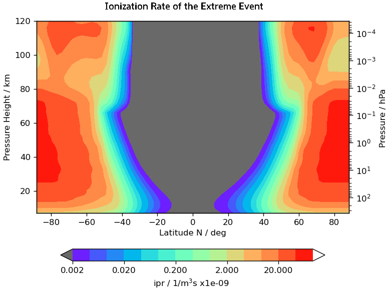
Figure 1The ionization rate of the extreme event (mean of 23–25 January 2009). One can clearly see the GMS component maximizing in the lower thermosphere following the auroral oval and the polar cap ionization by the SPE.
The impact of the solar events on ozone is mainly given by the particle-induced buildup of NOx which catalytically reacts with ozone. NOy, which includes all nitrogen containing species except N2O including the reservoir gases for NOx, has a very long lifetime in the stratosphere, where it contributes effectively to ozone destruction. In the middle atmosphere, the impact on ozone is the key parameter for any dynamical atmospheric impact of such events, as short-wave heating rates are dominated by ozone. Changes in ozone will change the temperature distribution in the middle atmosphere and the winds and propagating waves as a result. In addition, as the ozone density maximizes in the stratosphere, any reduction of ozone will also change the UV intensity at the surface. The SPE-induced ionization rate maximizes in the upper stratosphere and lower mesosphere; the GMS has its maximum ionization in the lower thermosphere. In order to estimate a possible maximum impact of a particular solar event, an appropriate dynamical situation would be where the portion of NOy built up in the mesosphere–lower thermosphere (MLT) during the event survives photochemical destruction and is transported into the lower stratosphere, where its lifetime is on the order of many years. This sets the date of such an experiment to the winter season.
In satellite observations from instruments like the Michelson Interferometer for Passive Atmospheric Sounding (MIPAS) on Envisat (Fischer et al., 2008) strong NOy intrusions from the lower thermosphere into the NH mesosphere and upper stratosphere have been observed after mid-winter sudden stratospheric warmings (SSWs) when accompanied by elevated stratosphere events. These show a strong downward transport of air from the MLT (Holt et al., 2013). For the NH, it has been shown that these events also yield the strongest ozone impact (Sinnhuber et al., 2018). In order to test if an extreme GMS can have a similar impact as the SPE, which maximizes lower in the mesosphere, we synchronize the SSW and the GMS. As an example of such a dynamical situation, we use the SSW of 21 January 2009, which has also been studied in the HEPPA-II experiment (Funke et al., 2017). We note that the situation in the Southern Hemisphere (SH) may be different. Here the polar middle atmosphere is essentially undisturbed for the whole winter, and an early intrusion from the MLT region may reach the mid-stratosphere. This has also been observed for the Antarctic winter 2003 (Funke et al., 2005).
In summary, the extreme event we study is a combination of a SPE and a GMS. The ionization rate is derived from observed events which have been scaled to a strength estimated for an event with a occurrence rate of yr−1 to yr−1, synchronized with an elevated stratosphere event.
For the purpose of this sensitivity study, we use the KArlsruhe SImulation Model of the middle Atmosphere (KASIMA; Kouker et al., 1999) in the version described in Sinnhuber et al. (2021). The model solves the meteorological basic equations in spectral form in the altitude range between 300 hPa and hPa, with pressure height (H=7 km and p0=1013.25 hPa) as a vertical coordinate. It uses radiative forcing terms for UV–Vis and IR as well as a gravity wave drag scheme. In order to yield a realistic meteorology, the model is relaxed (nudged) to ERA-Interim meteorological analyses (Dee et al., 2011) between the lower boundary of the model and 1 hPa. A full stratospheric chemistry including heterogeneous processes is adapted to include source terms related to particle ionization. For the production of HOx the parameterization of Solomon et al. (1981) is used. For the production of NOx, 0.7 NO molecules are produced per ion pair and 0.55 N atoms in ground state. The model also includes a HNO3 production from proton hydrates based on the parameterization of de Zafra and Smyshlyaev (2001), which has been modified to be dependent on actual ionization rates. The model was used in all the three HEPPA inter-comparisons (Funke et al., 2011a, 2017; Sinnhuber et al., 2021). The model has proven to realistically simulate chemistry in the middle atmosphere for NOy intrusions, which is sufficient for studying its direct impact.
The following simulations are performed: one with the extreme event (EXT), where the ionization rates from the extreme event are applied from 21 to 23 January, and one with a background ionization only (REF). The background ionization rate is a mean from AIMOS ionization rates (Wissing and Kallenrode, 2009) for minimum Ap indices. In addition, a simulation which only includes the solar proton event is used to compare the contributions of the two components.
4.1 NOy intrusion
Figure 2 shows the mean of NOy (= NOx + HNO3 + ClONO2 + BrONO2 + HONO + N2O5 + BrONO; gas phase only), where NOx = N + NO + NO2, over the northern polar cap (latitude >70∘ N) for 1 year with the dynamics and chemical boundary conditions of 2009 but with the extreme solar event described in Sect. 2 included. The two components of the event (SPE and GMS) can clearly be seen as an instantaneous increase over all altitudes and a tongue of increased NOy values transported from the MLT within the elevated stratopause event, respectively. In the specific dynamical situation, the downward transport of the GMS component from the MLT is fast enough to reach the photolytic “safe” stratosphere at the end of the NH winter which then causes a significant NOy enhancement in the upper stratosphere. It stays there and is diluted during the summer and is then transported further down in the beginning of the winter season. The enhancement related to the SPE is seen down to the tropopause and stays there over the whole year, with a relative enhancement of more than 20 %. NOx is lost through transport into the troposphere, where the main reservoir in the lowest stratosphere HNO3 is washed out, or into the mesosphere, where it is photolytically destroyed.
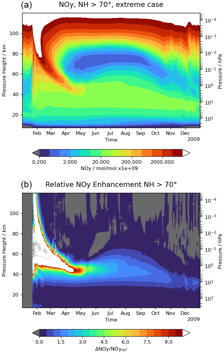
Figure 2(a) NOy mixing ratio in the course of 1 year with specified dynamics of the year 2009 (ERA-Interim) and applying the extreme scenario case as described in the text. For the polar cap, the intrusion connected to the MLT part dominates around the stratopause; below the stratopause NOy stems from the SPE. (b) Relative enhancement of NOy compared to the reference run.
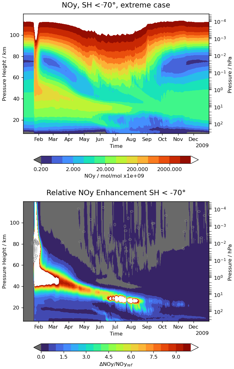
In the SH (shown in Fig. 3), the NOy enhancement is essentially from the SPE, as the MLT component is photolytically destroyed during the summer season. We also observe a higher relative enhancement here, as the excess NOy in the upper stratosphere is transported downward in the beginning of winter compared to the upward draft in the NH summer. In addition, de- and renitrification by sedimentation of condensed HNO3 can be observed, resulting in an effective removal of nitrate from the stratosphere into the troposphere. The relative maxima in the southern winter middle stratosphere are related to the higher supply of HNO3 at locations in the reference run where this air mass already was depleted.
The contribution of the GMS to the NOy at high northern latitudes (>70∘ N) in the intrusion is shown in Fig. 4. It is limited in altitude to above about 40 km and is diluted to values below 0.1 in autumn.
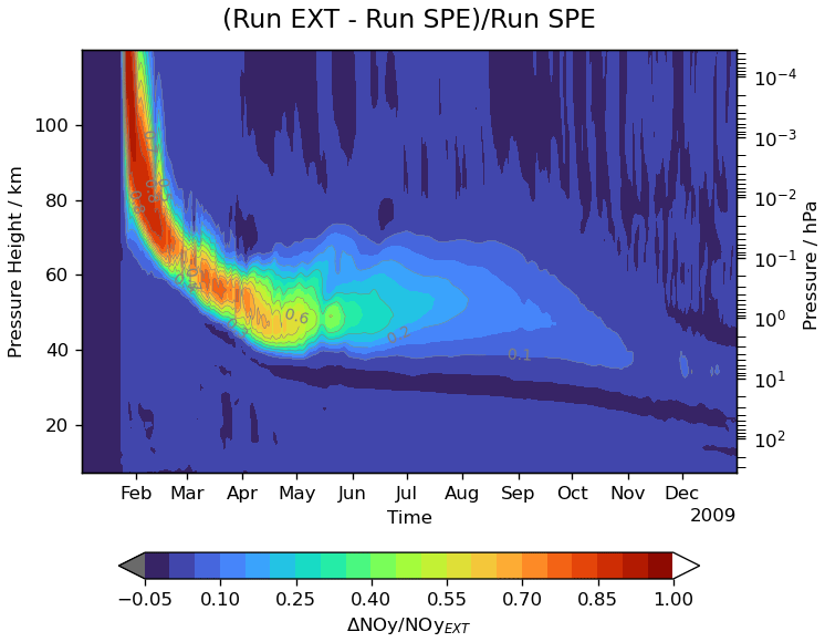
Figure 4The relative contribution of the GMS component to the NOy intrusion (latitude >70∘ N), calculated as the difference between the EXT run and a run with the SPE component only, relative to the full event.
The distribution of NOy over latitudes at 37 km altitude is shown in Fig. 5. At this altitude the contribution of NOy to ozone depletion maximizes (see, for example, Fig. 6.1 of Brasseur and Solomon, 2005). A closer inspection shows that at this altitude also NOy from the NH is transported to the SH and significantly contributes to the NOy after some months, as part of the diabatic circulation from the summer to the winter pole.

4.2 Impact on the global NOy budget
To assess the impact of the NOy intrusions on the global NOy budget, we first calculated the total column of NOy with and without the event, as shown in Fig. 6. The two hemispheres show remarkable differences, with a higher total relative NOy enhancement at high southern latitudes in the first 6 months but a fast decay after, in addition to a longer-lasting NOy enhancement in middle and high latitudes in the NH (see also Fig. 7). From Fig. 3, which shows mixing ratios, one can deduce that the strong relative enhancement is affected by differences in the depletion of gaseous NOy by denitrification in the reference and extreme run. This becomes clearer when showing the absolute change in the total columnar content. The change in the total amount NOy (in units of mol) for different latitude bands by the event is shown in Fig. 7. In the SH, we clearly observe the fast decay shortly after the event connected to the photolytical destruction in the polar mesosphere and then some stabilisation in the winter followed by the denitrification in the cold polar stratosphere. The NH is characterized by a more continuous decay, stabilizing in the next winter season.
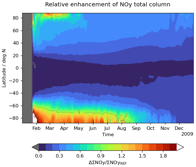
Figure 6Enhancement of the total NOy column (>7 km pressure height) relative to the reference run.

Figure 7The NOy signal from the extreme event (EXT-REF) for different latitude bands as the total amount of NOy in moles.
4.3 Impact on ozone
The NOy enhancement causes additional ozone depletion via the catalytic reaction of NOx with O3. This is shown in Fig. 8 as the relative change in ozone. In the MLT, there is also a short-lived ozone enhancement which is connected to the dissociation of O2 by atomic nitrogen. In addition, the ozone decrease in the stratosphere causes less absorption of solar UV and a small buildup of ozone below the depleted zone. Mirroring the different amount of NOy transported into the stratosphere, the corresponding ozone loss is higher in the SH, whereas the ozone loss in the NH lasts for a longer time. This just reflects the loss of NOy in the SH in the course of the polar winter.
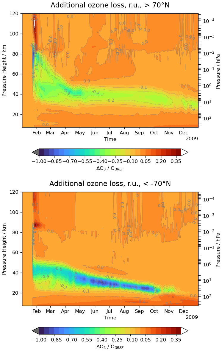
Figure 8Ozone change in the extreme run relative to the reference run ((REF-EXT)/REF) related to the NOy intrusion through the extreme event (EXT-REF) for the northern and southern polar caps (latitude ∘).
The change in the ozone column relative to the reference run is shown in Fig. 9. It shows the previously described asymmetry in the two hemispheres, with exceptional high changes of total ozone loss in the Antarctic vortex. Total ozone recovers to nearly normal values at the end of the simulation year in the SH. On the other hand, in the NH the maximum loss in the mid-latitudes is less than 5 %, but a deficit of total ozone of a few percent stays permanently throughout the year. The contribution of the GMS to the loss in total ozone is negligible (not shown).
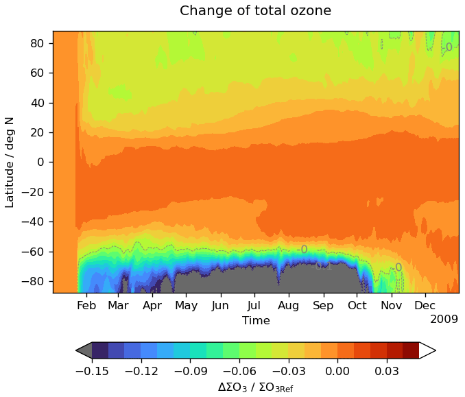
Figure 9The change in total ozone caused by the solar extreme event relative to the reference run.
5.1 Specific dynamical situation and the total NOy input
Inspecting Fig. 1, we note that the ionization rate of the GMS shows its maximum in the thermosphere and at the auroral oval latitudes, whereas the extreme solar particle event (ESPE) is concentrated to the poles. This has some consequences for the respective impacts of the two components. As discussed in Sect. 2, the specific dynamical situation maximizes the impact of solar extreme events in the NH via long-lasting downward transport of NOy in the winter polar middle atmosphere. Figure 4 shows that the contribution of the GMS to the additional NOy is of minor importance compared to the impact of the ESPE. The higher altitude of the source region together with its lower latitude makes the photochemical destruction of NOy at the end of the downward transport regime more probable. Accordingly, an additional experiment with a 10 × GMS event, but without the ESPE component, was carried out. In this event, NOy enhancement in the NH of about 2–3 Gmol in late summer is observed. We therefore conclude that an extreme GMS in the range discussed would not pose a strong and long-lasting disturbance in the NH middle atmosphere. Still, the mesospheric part of the ESPE benefits from this dynamical situation in the NH: NOy that has not reached the mid-stratosphere would have been destroyed photochemically when transported by an instable vortex or minor SSWs to the sunlit mid-latitudes.
For comparison, we also tested other dynamical situations, from early to late winter (only in the winter season is NOy stable in the mesosphere): in winter 2009–2010 but the event put on DOY 300 in 2009, a rather early and strong mid-winter warming (December 1998), and the SSW in mid-January 2004, the date of which being quite similar to the setup studied. For the EXT scenario, we estimate the initial total NOy input to about 65 Gmol which decreases to about 25 Gmol after 1 year (see Fig. 7). The undisturbed total NOy amount in the atmosphere prior to the event above about 7 km altitude is simulated to 135 Gmol. The experiments for 2004 and 1998 yield the same initial amount of the intrusion but decay to about 10 and 25 Gmol after 1 year, respectively. The event set to DOY 300 in 2009 yielded, with 53 Gmol, slightly less than the initial NOy and showed a rather fast decay to only a few gigamoles (Gmols) after 1 year.
Some insight might also be gained from comparison with Sukhodolov et al. (2017) (albeit their results are deduced from an ensemble mean and for pre-industrial conditions): their Fig. 4 shows a decay of the NOx enhancement to 100 % within about 140 d in the NH. In the EXT experiment after 140 d the enhancements still exceed 300 % and reach 100 % after about 270 d.
From these comparisons, the scenario selected seems to be an example of a strong and long-enduring impact of the event. Estimating the range of the impact of strong solar events under different dynamical situations requires additional simulations, including feedback effects on the dynamics. This is beyond the scope of this study and will be addressed in a follow-up paper.
The total NOy mass produced in experiment EXT of about 65 Gmol, corresponding to about 40 % of the total atmospheric NOy content, is substantially greater than what has been found in observation during the last decades. For example, Vitt and Jackman (1996) estimated a few percent increase of NOy after strong SPEs in the northern polar stratosphere, Funke et al. (2014) estimated the total NOy input from satellite observations for the period 2002 to 2012 to be a few gigamoles (Gmols) per year, and Reddmann et al. (2010) deduced the total NOy input from a model simulation for the period 2003 to 2004 to be about 2 Gmol. In terms of NOy input, the NOy buildup by the solar event studied is about 10 to 30 times higher than what is estimated for solar particle events observed in the satellite era, which is on the order of the scaling factor we apply to the ionization rates of the SPE. In this sense, the solar extreme event is also an atmospheric extreme.
The budget of NOy in the atmosphere in the longer term depends on the source strength of the event and the loss terms by photochemistry and exchange processes to the troposphere, where NOy is removed by precipitation.
For the source strength, we use ionization rates estimated for the event in 774 CE. There are several steps to estimate the ionization rates for such events which all have factors of uncertainty. This is extensively discussed in Usoskin et al. (2011) and in Sukhodolov et al. (2017). One of the main uncertainties of the SPE part is the energy spectrum of the protons which has been scaled from an event in 1956 with a rather hard spectrum compared to other events in the satellite era Usoskin et al. (2020). A softer spectrum would shift the maximum NOy production to higher altitudes, where the lifetime of NOy is reduced. Therefore, the initial NOy production by the ionization we estimate is probably on the upper limit of what can be expected.
The GMS contribution has been estimated from events observed in the past, but data at high flux levels are rare and have therefore substantial uncertainty. On the other hand, theoretical considerations (Vasyliunas, 2011) set an upper limit to the strength of a GMS in terms of Dst to about 2500 nT, which is probably outside of the estimations we used. In addition, the geographical distribution of the auroral oval depends on the strengths of the event. Here we used the distributions from the AISstorm model for observed events and therefore miss the shift of the auroral oval to lower latitudes when the GMS strength is much higher. The scaling factors taken from Meredith et al. (2016) have been derived for a particle population that is partly trapped in the magnetosphere. Applying them to particle precipitation includes another source of uncertainty. But even a contribution greater by a factor of 2 from the GMS part would not bring this component above the SPE contribution.
For the efficiency of NO production, we use in the model the results of Porter et al. (1976). Some studies indicate a dependency of these factors on the ionization rate itself (Nieder et al., 2014), with a kind of saturation effect, especially in the thermosphere. This can be a major uncertainty for the production term and needs detailed ion chemistry studies.
Besides the source strength, the downward transport from the source region in the mesosphere to the stratosphere is essential. From the studies within the SPARC HEPPA initative (Funke et al., 2011a, 2017), we know that many models do not correctly simulate this transport in the polar winter. The KASIMA model we use here in combination with ERA-Interim analyses yields downward transport from the MLT, which is generally in good agreement with observations, also for situations with an elevated stratosphere as we use here. Finally, the atmospheric lifetime of NOy is also determined by the correct pattern and strength of the Brewer–Dobson circulation. It determines the upward transport into the region with photolytic loss and the exchange to the troposphere. The mean age of air simulations found with KASIMA is also in good agreement with observations (Stiller et al., 2008; Haenel et al., 2015).
In conclusion, the main uncertainties for the strength of the NOy intrusion for a selected dynamical scenario as in our simulation are the energy spectrum of the particle flux and the initial ion chemistry production terms.
5.2 NOy loss through the Antarctic winter
The loss of NOy in the southern polar winter atmosphere deserves special attention. The KASIMA model includes heterogeneous processes in the polar winter stratosphere, causing denitrification and renitrification of the cold air masses in the Antarctic polar vortex through the nitric acid trihydrate (NAT) condensation of HNO3 on water ice and the adsorption on sulfate aerosols, followed by sedimentation of larger particles into the lower layers as part of the annual cycle. In the KASIMA model, this process seems to be saturated: in the core of the Antarctic polar vortex, denitrification is complete. Additional NOy brought into the lower stratosphere by the intrusion does not change this, but through the changed saturation pressure, greater volume will take part in denitrification. The change in total NOy for the southern polar cap in Fig. 7 supports this finding: at the end of the winter, most of the additional NOy of about 6 Gmol in the southern polar cap is lost to the troposphere.
Inspection of Fig. 3 shows that the majority of NOy renitrification in the southern polar lower stratosphere takes place between the end of July and the middle of August. NOy here is mainly in the form of HNO3. Once transported to the troposphere, NOy is deposited onto the surface by rain or snow within a few days. If we assume that the NOy is deposited in the form of NO3 on the southern polar cap, we deduce an average deposition value of g cm−2. Using the approximation that the column-integrated particle produced NOy is deposited, Melott et al. (2016) estimate a deposition of about g cm−2 for the 1956 event, corresponding to g cm−2 for the extreme event just by applying the scaling factor. As in our model, loss processes such as photolysis and transport to lower latitudes are included, and our lower value is in line with their estimation. With an average precipitation of 166 mm yr−1 for Antarctica and assuming that the nitrate is deposited within 1 month, we estimate a mass mixing ratio for nitrate of 190 ng g−1 in a monthly layer of (evenly distributed) deposited snow. A typical detection limit for nitrate events measured in ice cores with monthly-to-sub-annual resolution is on the order of 100 ng g−1 (Smart et al., 2014), so we would expect that a nitrate signal would be observable for such an event in Antarctica. Note that our model does not include tropospheric meteorology, so an analysis of regional precipitation patterns is outside the scope of this paper. Sukhodolov et al. (2017) estimate from their analysis that a nitrate signal would not be detectable in a Greenland ice core. This is essentially in agreement with our findings, which show a much smaller change in total NOy in the northern polar cap in early spring. Here, the higher polar temperatures and less stable polar vortex do not allow for strong and fast denitrification, the primary cause of the high NOy depletion in the southern polar lower stratosphere. In addition, we use analyzed winds and temperatures similar to realistic meteorology, whereas free-running models may fail in several ways to correctly describe the polar dynamical and chemical processes in the lower stratosphere. For the case of the 774/5 event, ice core data for Antarctica do not show nitrate enhancements (Sukhodolov et al., 2017; Jong et al., 2022). From Fig. 3 one may note that a strong denitrification signal is only expected when the NOy tongue reaches the lower stratosphere when there are also low temperatures. A mismatch, for example an event occurring in Antarctic spring, would presumably result in a much broader and therefore undetectable nitrate peak.
5.3 Ozone loss caused by the event
Inspecting Fig. 8, one may note the nearly complete ozone loss immediately after the event in the polar mesosphere. This raises the questions of the extent that the ozone loss scales with the NOy enhancement and if the loss is near saturation, at least during the first weeks after the event. For this reason, we performed an additional sensitivity experiment where we scaled the strength of the ionization rates of the EXT experiment by a factor of 0.2. Figure 10 gives the result of this experiment for the NH in terms of the total amount of the enhancement of NOy and the corresponding ozone decrease. First, we can see that the total NOy input into the atmosphere scales nearly perfectly with the strength of the forcing. Surprisingly, the ozone decrease also scales with the ionization rate by about the same factor, with a only slightly relative higher ozone decrease in the reduced case. In addition, the ozone loss is strongly correlated with the additional NOy.
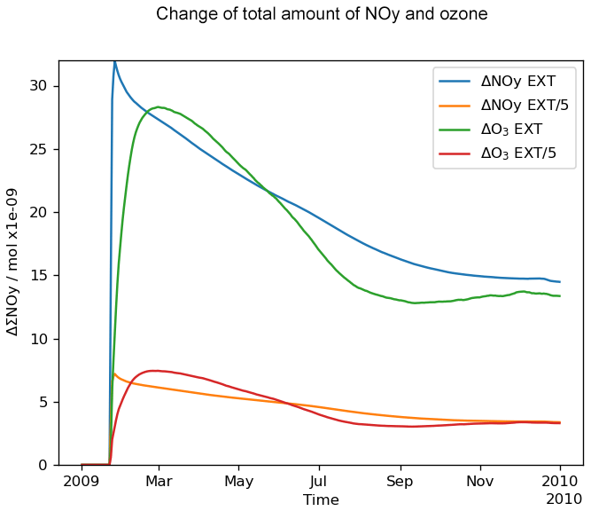
Figure 10Total NOy input by the EXT event and an event with a strength of (in Gmols) into the NH. The corresponding decrease of the ozone (in Gmols), scaled by a factor of −0.03, is also shown.
The reason for this behaviour lies in the fact that the ESPE reaches deep into the middle atmosphere, where the relative ozone reduction related to enhanced NOy is small; again, see Fig. 2. For total ozone, which essentially stems from the lower stratosphere, this results in quasi-linear scaling of ΔNOy and ΔO3.
Considering radiative feedback effects, the situation may be different: following Gray et al. (2010), an efficient top-down mechanism for radiative feedback involves temperature gradients induced by ozone changes in the mid-latitudes around the stratopause. For our setup, the induced decrease of the ozone amount above 40 km for latitudes >40∘ N shows a more saturated scaling (3× instead of 5×) and vanishes after about 1 year, whereas the total ozone loss stays at a constant level in the second half of the year, stemming mainly from the lower stratosphere. In our setup, we would therefore expect only smaller feedback on the circulation compared to the setup of Sukhodolov et al. (2017).
5.4 Increase of UV index caused by the ozone loss
In order to estimate a health-related impact caused by the reduced total ozone column, we calculate the corresponding change in the UV index (UVI). The UVI is calculated from the spectrally weighted and integrated solar irradiance, where the weight function takes the erythemal action spectrum into account (CIE International Commission on Illumination, 2019). Here we use the simplified formula of Allaart et al. (2004), their Eq. (8) together with Eq. (6), to estimate the increase of UVI connected to the decrease of the total ozone column (ΣO3) after a solar extreme event. In this formula, besides the dependence on the extraterrestrial flux and the solar zenith angle, for cloud-free situations, UVI depends on ΣO3 only. For the column down to 7 km, the lower boundary of the model, we obtain an increase of the UVI for noon, as shown in Fig. 11. The absolute highest change of about 0.5 UVI occurs in the months of March and April at the latitude of 25∘ N, which includes the region on Earth with the highest population density. The relative change in the UVI reaches about 4 %–5 % in the northern mid-latitudes, where the summer months are also affected. In order to put this change in context, we remark that the ozone depletion by chlorofluorocarbons reached a maximum reduction of total ozone of about 3 % in the northern mid-latitudes in 1995 (Weber et al., 2022), quite similar to the values we found for the extreme event (see Fig. 9) but lasting for more than a decade.
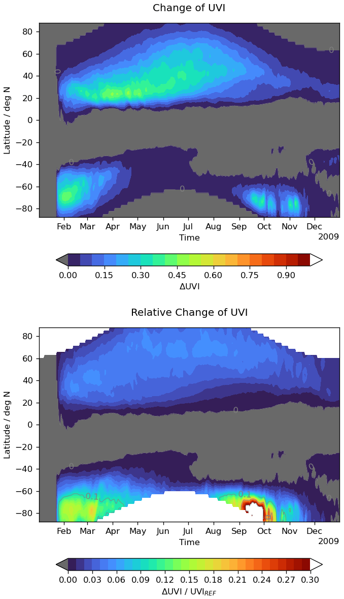
There is also a significant increase of UVI at high southern latitudes but not at latitudes which have high population density.
The purpose of this study was to analyze the direct effects of an extreme solar eruption on the chemical state of the middle atmosphere. We considered an extreme solar event with a strong SPE that was also connected with a strong GMS. The setup of the numerical experiment was chosen to yield a maximum chemical impact in the NH. This was achieved by setting the event to NH winter in combination with an elevated stratosphere SSW event. The main findings are that the GMS component from energetic electrons even in this dynamical situation leads only to a minor ozone reduction. The ozone reduction in our extreme scenario stems essentially from the ESPE and survives through the following boreal summer. The additional NOy amount in the middle atmosphere scales with the strength of the event, as does the ozone loss. The studied event yields a significant but limited enhancement of the UVI in populated latitudes in the first months following the event of a few percent. The ESPE causes a strong impact in terms of additional NOy and ozone loss in southern high latitudes, despite the event having been put to NH winter to minimize photochemical loss of NOy. This is related to the deep penetration of energetic particles at altitudes where the loss of NOy is negligible and also to the early onset of downward transport with the beginning of Antarctic winter in the middle atmosphere. Besides the related ozone loss, the denitrification of NOy in the lower Antarctic stratosphere and the following washout in the troposphere can yield potentially measurable NO3 signals in ice cores. This, however, has not been observed to date, perhaps because the signal strength strongly depends on the timing of the event. Therefore, nitrate signals in ice cores are not reliable indicators of solar activity.
Model data used for this analysis are accessible through https://doi.org/10.35097/1104 (Reddmann, 2023).
TR prepared the experiments and wrote the paper; IU, JMW, and OY provided the ionization rates; and MS critically discussed and improved the manuscript.
The contact author has declared that none of the authors has any competing interests.
Publisher's note: Copernicus Publications remains neutral with regard to jurisdictional claims in published maps and institutional affiliations.
The authors acknowledge the NOAA National Centers for Environmental Information (https://ngdc.noaa.gov/stp/satellite/poes/dataaccess.html, last access: June 2023) for the POES and Metop particle data used in this study.
This work was supported by the German Federal Ministry of Education and Research within the research
program ROMIC-2 (project SOLCHECK, grant
no. 01LG1906D) and by the Academy of Finland (project ESPERA, grant no. 321882). The AIMOS model is funded by the German Science Foundation (DFG project no. WI4417/2-1). Jan Maik
Wissing also acknowledges support by the German Aerospace Center (DLR).
The article processing charges for this open-access publication were covered by the Karlsruhe Institute of Technology (KIT).
This paper was edited by John Plane and reviewed by two anonymous referees.
Allaart, M., van Weele, M., Fortuin, P., and Kelder, H.: An empirical model to predict the UV-index based on solar zenith angles and total ozone, Meteorol. Appl., 11, 59–65, https://doi.org/10.1017/S1350482703001130, 2004. a
Aschwanden, M. J., Caspi, A., Cohen, C. M. S., Holman, G., Jing, J., Kretzschmar, M., Kontar, E. P., McTiernan, J. M., Mewaldt, R. A., O'Flannagain, A., Richardson, I. G., Ryan, D., Warren, H. P., and Xu, Y.: Global Energetics of Solar Flares. V. Energy Closure in Flares and Coronal Mass Ejections, Astrophys. J., 836, 17, https://doi.org/10.3847/1538-4357/836/1/17, 2017. a
Brasseur, G. P. and Solomon, S.: Aeronomy of the Middle Atmosphere, Springer, 3rd Edn., ISBN-10 1-4020-3284-6, 2005. a
Calisto, M., Usoskin, I., Rozanov, E., and Peter, T.: Influence of Galactic Cosmic Rays on atmospheric composition and dynamics, Atmos. Chem. Phys., 11, 4547–4556, https://doi.org/10.5194/acp-11-4547-2011, 2011. a
Carrington, R. C.: Description of a Singular Appearance seen in the Sun on September 1, 1859, Mon. Not. R. Astron. Soc., 20, 13–15, 1859. a
CIE International Commission on Illumination: ISO/CIE 17166:2019 Erythema reference action spectrum and standard erythema dose, ISO, 2019. a
Cliver, E. W., Schrijver, C. J., Shibata, K., and Usoskin, I. G.: Extreme solar events, Living Rev. Sol. Phys., 19, 1–143, 2022. a, b
de Zafra, R. and Smyshlyaev, S.: On the formation of HNO3 in the Antarctic mid to upper stratosphere in winter, J. Geophys. Res., 106, 23115–23125, 2001. a
Dee, D. P., Uppala, S. M., Simmons, A. J., Berrisford, P., Poli, P., Kobayashi, S., Andrae, U., Balmaseda, M. A., Balsamo, G., Bauer, P., Bechtold, P., Beljaars, A. C. M., van de Berg, L., Bidlot, J., Bormann, N., Delsol, C., Dragani, R., Fuentes, M., Geer, A. J., Haimberger, L., Healy, S. B., Hersbach, H., Hólm, E. V., Isaksen, L., Kållberg, P., Köhler, M., Matricardi, M., McNally, A. P., Monge-Sanz, B. M., Morcrette, J.-J., Park, B.-K., Peubey, C., de Rosnay, P., Tavolato, C., Thépaut, J.-N., and Vitart, F.: The ERA-Interim reanalysis: configuration and performance of the data assimilation system, Q. J. Roy. Meteor. Soc., 137, 553–597, https://doi.org/10.1002/qj.828, 2011. a
Fischer, H., Birk, M., Blom, C., Carli, B., Carlotti, M., von Clarmann, T., Delbouille, L., Dudhia, A., Ehhalt, D., Endemann, M., Flaud, J. M., Gessner, R., Kleinert, A., Koopman, R., Langen, J., López-Puertas, M., Mosner, P., Nett, H., Oelhaf, H., Perron, G., Remedios, J., Ridolfi, M., Stiller, G., and Zander, R.: MIPAS: an instrument for atmospheric and climate research, Atmos. Chem. Phys., 8, 2151–2188, https://doi.org/10.5194/acp-8-2151-2008, 2008. a
Funke, B., López-Puertas, M., Gil-López, S., von Clarmann, T., Stiller, G. P., Fischer, H., and Kellmann, S.: Downward transport of upper atmospheric NOx into the polar stratosphere and lower mesosphere during the Antarctic 2003 and Arctic 2002/2003 winters, J. Geophys. Res.-Atmos., 110, D24308, https://doi.org/10.1029/2005JD006463, 2005. a
Funke, B., Baumgaertner, A., Calisto, M., Egorova, T., Jackman, C. H., Kieser, J., Krivolutsky, A., López-Puertas, M., Marsh, D. R., Reddmann, T., Rozanov, E., Salmi, S.-M., Sinnhuber, M., Stiller, G. P., Verronen, P. T., Versick, S., von Clarmann, T., Vyushkova, T. Y., Wieters, N., and Wissing, J. M.: Composition changes after the “Halloween” solar proton event: the High Energy Particle Precipitation in the Atmosphere (HEPPA) model versus MIPAS data intercomparison study, Atmos. Chem. Phys., 11, 9089–9139, https://doi.org/10.5194/acp-11-9089-2011, 2011. a, b, c
Funke, B., Lopez-Puertas, M., Holt, L., Randall, C. E., Stiller, G. P., and von Clarmann, T.: Hemispheric distributions and interannual variability of NOy produced by energetic particle precipitation in 2002–2012, J. Geophys. Res.-Atmos., 119, 13565–13582, https://doi.org/10.1002/2014JD022423, 2014. a
Funke, B., Ball, W., Bender, S., Gardini, A., Harvey, V. L., Lambert, A., López-Puertas, M., Marsh, D. R., Meraner, K., Nieder, H., Päivärinta, S.-M., Pérot, K., Randall, C. E., Reddmann, T., Rozanov, E., Schmidt, H., Seppälä, A., Sinnhuber, M., Sukhodolov, T., Stiller, G. P., Tsvetkova, N. D., Verronen, P. T., Versick, S., von Clarmann, T., Walker, K. A., and Yushkov, V.: HEPPA-II model–measurement intercomparison project: EPP indirect effects during the dynamically perturbed NH winter 2008–2009, Atmos. Chem. Phys., 17, 3573–3604, https://doi.org/10.5194/acp-17-3573-2017, 2017. a, b, c, d
Gray, L. J., Beer, J., Geller, M., Haigh, J. D., Lockwood, M., Matthes, K., Cubasch, U., Fleitmann, D., Harrison, G., Hood, L., Luterbacher, J., Meehl, G. A., Shindell, D., van Geel, B., and White, W.: SOLAR INFLUENCES ON CLIMATE, Rev. Geophys., 48, RG4001, https://doi.org/10.1029/2009RG000282, 2010. a
Haenel, F. J., Stiller, G. P., von Clarmann, T., Funke, B., Eckert, E., Glatthor, N., Grabowski, U., Kellmann, S., Kiefer, M., Linden, A., and Reddmann, T.: Reassessment of MIPAS age of air trends and variability, Atmos. Chem. Phys., 15, 13161–13176, https://doi.org/10.5194/acp-15-13161-2015, 2015. a
Holt, L. A., Randall, C. E., Peck, E. D., Marsh, D. R., Smith, A. K., and Harvey, V. L.: The influence of major sudden stratospheric warming and elevated stratopause events on the effects of energetic particle precipitation in WACCM, J. Geophys. Res.-Atmos., 118, 11–636, 2013. a
Jong, L. M., Plummer, C. T., Roberts, J. L., Moy, A. D., Curran, M. A. J., Vance, T. R., Pedro, J. B., Long, C. A., Nation, M., Mayewski, P. A., and van Ommen, T. D.: 2000 years of annual ice core data from Law Dome, East Antarctica, Earth Syst. Sci. Data, 14, 3313–3328, https://doi.org/10.5194/essd-14-3313-2022, 2022. a
Kouker, W., Langbein, I., Reddmann, T., and Ruhnke, R.: The Karlsruhe Simulation Model of The Middle Atmosphere Version 2, Wiss. Ber. FZKA 6278, Forsch. Karlsruhe, Karlsruhe, Germany, 1999. a
Maliniemi, V., Asikainen, T., and Mursula, K.: Spatial distribution of Northern Hemisphere winter temperatures during different phases of the solar cycle, J. Geophys. Res.-Atmos., 119, 9752–9764, https://doi.org/10.1002/2013JD021343, 2014. a
Mekhaldi, F., Adolphi, F., Herbst, K. and Muscheler, R.: The Signal of Solar Storms Embedded in Cosmogenic Radionuclides: Detectability and Uncertainties, J. Geophys. Res.-Space, 126, e2021JA029351, https://doi.org/10.1029/2021JA029351, 2021. a
Melott, A. L., Thomas, B. C., Laird, C. M., Neuenswander, B., and Atri, D.: Atmospheric ionization by high-fluence, hard-spectrum solar proton events and their probable appearance in the ice core archive, J. Geophys. Res.-Atmos., 121, 3017–3033, https://doi.org/10.1002/2015JD024064, cited By 16, 2016. a
Meredith, N. P., Horne, R. B., Isles, J. D., and Green, J. C.: Extreme energetic electron fluxes in low Earth orbit: Analysis of POES E > 30, E > 100, and E > 300 keV electrons, Adv. Space Res., 14, 136–150, https://doi.org/10.1002/2015SW001348, 2016. a, b, c, d
Nesse Tyssøy, H., Sinnhuber, M., Asikainen, T., Bender, S., Clilverd, M. A., Funke, B., van de Kamp, M., Pettit, J. M., Randall, C. E., Reddmann, T., Rodger, C. J., Rozanov, E., Smith-Johnsen, C., Sukhodolov, T., Verronen, P. T., Wissing, J. M., and Yakovchuk, O.: HEPPA III Intercomparison Experiment on Electron Precipitation Impacts: 1. Estimated Ionization Rates During a Geomagnetic Active Period in April 2010, J. Geophys. Res., 127, e2021JA029128, https://doi.org/10.1029/2021JA029128, 2021. a
Nieder, H., Winkler, H., Marsh, D. R., and Sinnhuber, M.: NOx production due to energetic particle precipitation in the MLT region: Results from ion chemistry model studies, J. Geophys. Res., 119, 2137–2148, https://doi.org/10.1002/2013JA019044, 2014. a
Pettit, J., Randall, C. E., Marsh, D. R., Bardeen, C. G., Qian, L., Jackman, C. H., Woods, T. N., Coster, A., and Harvey, V. L.: Effects of the September 2005 Solar Flares and Solar Proton Events on the Middle Atmosphere in WACCM, J. Geophys. Res., 123, 5747–5763, https://doi.org/10.1029/2018JA025294, 2018. a
Porter, H. S., Jackman, C. H., and Green, A. E. S.: Efficiencies for production of atomic nitrogen and oxygen by relativistic proton impact in air, J. Chem. Phys, 65, 154–167, https://doi.org/10.1063/1.432812, 1976. a
Reddmann, T.: Model results of solar extreme scenarios with the KASIMA model, RADAR4KIT [data set], https://doi.org/10.35097/1104, 2023. a
Reddmann, T., Ruhnke, R., Versick, S., and Kouker, W.: Modeling disturbed stratospheric chemistry during solar-induced NOx enhancements observed with MIPAS/ENVISAT, J. Geophys. Res., 115, D00111, https://doi.org/10.1029/2009JD012569, 2010. a
Seppälä, A., Randall, C. E., Clilverd, M. A., Rozanov, E., and Rodger, C. J.: Geomagnetic activity and polar surface air temperature variability, J. Geophys. Res., 114, A10312, https://doi.org/10.1029/2008JA014029, 2009. a
Sinnhuber, M., Nieder, H., and Wieters, N.: Energetic Particle Precipitation and the Chemistry of the Mesosphere/Lower Thermosphere, Surv. Geophys., 33, 1281–1334, https://doi.org/10.1007/s10712-012-9201-3, 2012. a
Sinnhuber, M., Berger, U., Funke, B., Nieder, H., Reddmann, T., Stiller, G., Versick, S., von Clarmann, T., and Wissing, J. M.: NOy production, ozone loss and changes in net radiative heating due to energetic particle precipitation in 2002–2010, Atmos. Chem. Phys., 18, 1115–1147, https://doi.org/10.5194/acp-18-1115-2018, 2018. a
Sinnhuber, M., Nesse Tyssoy, H., Asikainen, T., Bender, S., Funke, B., Hendrickx, K., Pettit, J. M., Reddmann, T., Rozanov, E., Schmidt, H., Smith-Johnsen, C., Sukhodolov, T., Szelag, M. E., van de Kamp, M., Verronen, P. T., Wissing, J. M., and Yakovchuk, O. S.: Heppa III Intercomparison Experiment on Electron Precipitation Impacts: 2. Model-Measurement Intercomparison of Nitric Oxide (NO) During a Geomagnetic Storm in April 2010, J. Geophys. Res., 126, e2021JA029466, https://doi.org/10.1029/2021JA029466, 2021. a, b, c
Smart, D. F., Shea, M. A., Melott, A. L., and Laird, C. M.: Low time resolution analysis of polar ice cores cannot detect impulsive nitrate events, J. Geophys. Res., 119, 9430–9440, https://doi.org/10.1002/2014JA020378, 2014. a
Solomon, S., Rusch, D. W., Gérard, J.-C., Reid, G. C., and Crutzen, P. J.: The effect of particle precipitation events on the neutral and ion chemistry of the middle atmosphere: II. Odd hydrogen, Planet. Space Sci., 29, 885–893, 1981. a
Stiller, G. P., von Clarmann, T., Höpfner, M., Glatthor, N., Grabowski, U., Kellmann, S., Kleinert, A., Linden, A., Milz, M., Reddmann, T., Steck, T., Fischer, H., Funke, B., López-Puertas, M., and Engel, A.: Global distribution of mean age of stratospheric air from MIPAS SF6 measurements, Atmos. Chem. Phys., 8, 677–695, https://doi.org/10.5194/acp-8-677-2008, 2008. a
Sukhodolov, T., Usoskin, I., Rozanov, E., Asvestari, E., Ball, W. T., Curran, M. A. J., Fischer, H., Kovaltsov, G., Miyake, F., Peter, T., Plummer, C., Schmutz, W., Severi, M., and Traversi, R.: Atmospheric impacts of the strongest known solar particle storm of 775 AD, Sci. Rep., 7, 45257, https://doi.org/10.1038/srep45257, 2017. a, b, c, d, e, f, g
Usoskin, I., Koldobskiy, S., Kovaltsov, G. A., Gil, A., Usoskina, I., Willamo, T., and Ibragimov, A.: Revised GLE database: Fluences of solar energetic particles as measured by the neutron-monitor network since 1956, Astron. Astrophys., 640, A17, https://doi.org/10.1051/0004-6361/202038272, 2020. a
Usoskin, I. G.: A history of solar activity over millennia, Living Rev. Sol. Phys., 14, 3, https://doi.org/10.1007/s41116-017-0006-9, 2017. a, b
Usoskin, I. G., Kovaltsov, G. A., Mironova, I. A., Tylka, A. J., and Dietrich, W. F.: Ionization effect of solar particle GLE events in low and middle atmosphere, Atmos. Chem. Phys., 11, 1979–1988, https://doi.org/10.5194/acp-11-1979-2011, 2011. a, b
Vasyliunas, V. M.: The largest imaginable magnetic storm, J. Atmos. Sol.-Terr. Phy., 73, 1444–1446, https://doi.org/10.1016/j.jastp.2010.05.012, 2011. a
Vitt, F. M. and Jackman, C. H.: A comparison of sources of odd nitrogen production from 1974 through 1993 in the Earth's middle atmosphere as calculated using a two-dimensional model, J. Geophys. Res.-Atmos., 101, 6729–6739, https://doi.org/10.1029/95JD03386, 1996. a
Weber, M., Arosio, C., Coldewey-Egbers, M., Fioletov, V. E., Frith, S. M., Wild, J. D., Tourpali, K., Burrows, J. P., and Loyola, D.: Global total ozone recovery trends attributed to ozone-depleting substance (ODS) changes derived from five merged ozone datasets, Atmos. Chem. Phys., 22, 6843–6859, https://doi.org/10.5194/acp-22-6843-2022, 2022. a
Wissing, J. M. and Kallenrode, M. B.: Atmospheric Ionization Module Osnabruck (AIMOS): A 3-D model to determine atmospheric ionization by energetic charged particles from different populations, J. Geophys. Res., 114, A06104, https://doi.org/10.1029/2008JA013884, 2009. a