the Creative Commons Attribution 4.0 License.
the Creative Commons Attribution 4.0 License.
 | 16 Jan 2023
Climate response to off-equatorial stratospheric sulfur injections in three Earth system models – Part 2: Stratospheric and free-tropospheric response
Daniele Visioni
Ben Kravitz
Andy Jones
James M. Haywood
Jadwiga Richter
Douglas G. MacMartin
Peter Braesicke
The paper constitutes Part 2 of a study performing a first systematic inter-model comparison of the atmospheric responses to stratospheric aerosol injection (SAI) at various single latitudes in the tropics, as simulated by three state-of-the-art Earth system models – CESM2-WACCM6, UKESM1.0, and GISS-E2.1-G. Building on Part 1 (Visioni et al., 2023) we demonstrate the role of biases in the climatological circulation and specific aspects of the model microphysics in driving the inter-model differences in the simulated sulfate distributions. We then characterize the simulated changes in stratospheric and free-tropospheric temperatures, ozone, water vapor, and large-scale circulation, elucidating the role of the above aspects in the surface SAI responses discussed in Part 1.
We show that the differences in the aerosol spatial distribution can be explained by the significantly faster shallow branches of the Brewer–Dobson circulation in CESM2, a relatively isolated tropical pipe and older tropical age of air in UKESM, and smaller aerosol sizes and relatively stronger horizontal mixing (thus very young stratospheric age of air) in the two GISS versions used. We also find a large spread in the magnitudes of the tropical lower-stratospheric warming amongst the models, driven by microphysical, chemical, and dynamical differences. These lead to large differences in stratospheric water vapor responses, with significant increases in stratospheric water vapor under SAI in CESM2 and GISS that were largely not reproduced in UKESM. For ozone, good agreement was found in the tropical stratosphere amongst the models with more complex microphysics, with lower stratospheric ozone changes consistent with the SAI-induced modulation of the large-scale circulation and the resulting changes in transport. In contrast, we find a large inter-model spread in the Antarctic ozone responses that can largely be explained by the differences in the simulated latitudinal distributions of aerosols as well as the degree of implementation of heterogeneous halogen chemistry on sulfate in the models.
The use of GISS runs with bulk microphysics demonstrates the importance of more detailed treatment of aerosol processes, with contrastingly different stratospheric SAI responses to the models using the two-moment aerosol treatment; however, some problems in halogen chemistry in GISS are also identified that require further attention. Overall, our results contribute to an increased understanding of the underlying physical mechanisms as well as identifying and narrowing the uncertainty in model projections of climate impacts from SAI.
- Article
(14484 KB) - Full-text XML
- Companion paper
-
Supplement
(5032 KB) - BibTeX
- EndNote


Observations of the cooling produced by past explosive volcanic eruptions (Robock, 2000) have prompted numerous investigations into the feasibility and risks of artificially injecting SO2 in the lower stratosphere in order to partially counteract the effect of rising greenhouse gases (Crutzen, 2006); this is usually termed stratospheric aerosol injection (SAI) or solar geoengineering. The formation of sulfate aerosols after SO2 oxidation prevents a portion of the incoming sunlight from reaching the troposphere, thus cooling the surface. However, this is not the only effect that would be produced from sulfate aerosols in the Earth system (e.g., Visioni et al., 2021). The localized heating of the lower stratosphere would modify the local chemical composition of the atmosphere and alter the large-scale atmospheric circulation. These side effects can thus modify the direct response to SAI, further modulating the radiative balance as well as impacting regional climate and ecosystems. Yet, past investigations of these most often focused on one single model. For instance, Ferraro et al. (2015) analyzed the impacts of a tropical sulfate injection on stratospheric dynamics in the University of Reading Intermediate General Circulation Model (IGCM). Tilmes et al. (2017, 2018b) and Richter et al. (2017) analyzed the atmospheric response to injections at different latitudes and/or altitudes in the Community Earth System Model 1 (CESM1) with the Whole Atmosphere Community Climate Model (WACCM) as its atmospheric component (CESM1-WACCM) in order to understand the underlying mechanisms in the climate response.
However, models are themselves imperfect, and hence model intercomparisons are useful in understanding uncertainties in climate responses to SAI. Such uncertainties arise from many sources, including the efficiency of SO2 to aerosol conversion, the extent to which sulfate aerosols will be transported away from the injection locations by the large-scale circulation and mixing processes, the removal of aerosols from the atmosphere altogether, and the efficiency of the direct impacts of aerosols on the radiative balance, as well as from uncertainties in any indirect impacts, for instance on atmospheric circulations and clouds. Simulations with a number of different models can thus help represent the uncertainty in real-world climate responses to a hypothetical SAI deployment, whilst identifying and attributing certain characteristics of individual model responses to particular aspects of model design or features can help narrow this real-world uncertainty. Several of such intercomparison studies were carried out as a part of the Geoengineering Model Intercomparison Project (GeoMIP, Kravitz et al., 2011, 2015). However, the implementation of the experimental protocols often differed between the participating climate models, which hindered confident attribution of drivers of the inter-model spread. Pitari et al. (2014) found large differences in the simulated stratospheric ozone responses in the GeoMIP G4 experiment, which were partially related to different profiles of the latitudinal distribution of sulfate aerosols used in various models. Tilmes et al. (2022) examined the impacts of SAI on the future evolution of stratospheric ozone using the three Earth system models (ESMs) with interactive chemistry participating in the GeoMIP G6 experiment. However, only two out of the three models included an interactive aerosol scheme, while the third model prescribed the aerosol optical depth (AOD) from the G4SSA experiment (Tilmes et al., 2015). Moreover, even for these two models, both the location of injections (0∘ at 25 km for CESM and 10∘ S–10∘ N at 18 km for UKESM) and the yearly amounts of SO2 injected (the injection rates were modified to achieve an amount of cooling corresponding to the model difference between the Shared Socioeconomic Pathway, SSP, 5–8.5 and 2–4.5 scenarios; Meinshausen et al., 2020) varied considerably.
Finally, rather than injecting fixed amounts of SO2, some recent studies examined the climate response to SAI in CESM1-WACCM using a feedback algorithm that injected varied amounts of SO2 at four off-equatorial locations in order to control not only the global mean surface temperature but also the Equator-to-pole and interhemispheric temperature gradients (e.g., Tilmes et al., 2018a). This approach has been shown to result in a more uniform surface cooling and thus fewer side effects than an equatorial injection strategy (Kravitz et al., 2019). Providing the basis for replicating this approach in other climate models is one of the goals of the experiments described here, as detailed in the companion paper (Visioni et al., 2023; hereafter Part 1). Such a multi-model comparison will provide insights into the climatic impacts of a more complex, time-varying SAI strategy aimed at reducing some of the surface side effects of a potential deployment. However, understanding inter-model differences in the simulated responses in such experiments could present its own challenges due to likely different magnitudes and distributions of the simulated SO2 injections amongst the models and thus differences in the stratospheric responses and their contribution to the surface climate changes.
The study presented here avoids these issues by examining a set of carefully designed sensitivity experiments with fixed point injections of SO2 in the lower stratosphere at single latitudes in the tropics. We use three comprehensive ESMs that were previously used to inform a range of past and future climate studies and that participated in the CMIP6 intercomparison, i.e., CESM version 2 with WACCM6 as its atmospheric component (CESM2-WACCM6), the United Kingdom Earth System Model (UKESM1.0), and the NASA Goddard Institute for Space Studies model (GISS-E2.1-G). By keeping the simulated SO2 emissions in the model experiments as similar as possible, we aim to robustly identify the similarities and differences in the simulated responses amongst the models, as well as identify and attribute the drivers of these differences. Such an exercise aims to improve our understanding of the sources of uncertainty in climate model projections of SAI and identify areas of future model improvements. In addition, as mentioned above, characterizing model responses to fixed SO2 injections and origins of inter-model differences will also help our understanding of the simulated responses in more complex scenarios of SAI deployment employing a feedback algorithm.
Part 1 analyzed the simulated aerosol fields and their relationships to the surface temperature and precipitation responses in these experiments. Here we build on these findings by elucidating the contribution of biases in model transport to the simulated sulfate distributions, in addition to further illustrating aspects of aerosol microphysics. We then characterize the simulated changes in stratospheric and free-tropospheric temperatures, ozone, water vapor, and large-scale circulation, elucidating the role of the above aspects in the surface SAI responses discussed in Part 1. We also identify commonalities and differences in the simulated responses, and by doing so we elucidate whether the main findings of Tilmes et al. (2018b) and Richter et al. (2017) utilizing CESM1-WACCM can be reproduced in a multi-model framework. Section 2 summarizes the model simulations performed. In Sect. 3.1 we focus on the simulated sulfate aerosol distributions, and we evaluate and discuss the role of biases in model transport in contributing to the inter-model spread. We then discuss the associated SAI impacts on stratospheric temperatures (Sect. 3.2), ozone, large-scale residual circulation (Sect. 3.3), water vapor (Sect. 3.4), and zonal winds (Sect. 3.5). Finally, Sect. 4 summarizes and discusses the main results.
2.1 Experimental description
A detailed description of the ESMs used and the simulations performed can be found in Part 1. Briefly, we use CESM2-WACCM6 (Gettelman et al., 2019; Danabasoglu et al., 2020, thereafter CESM2), UKESM1.0 (Sellar et al., 2019; Archibald et al., 2020; thereafter UKESM), and GISS-E2.1-G (Kelley et al., 2020). Both CESM2 and UKESM use modal two-moment aerosol microphysical schemes that account for the evolution of both aerosol mass and size distribution. For GISS-E2.1-G, we use two versions differing only in the aerosol scheme, i.e., the two-moment MATRIX (Multiconfiguration Aerosol TRacker of mIXing state) scheme with Aitken and accumulation aerosol modes (Bauer et al., 2008, 2020; hereafter GISS-MATRIX) and the bulk aerosol OMA (One-Moment Aerosol) scheme (Koch et al., 2006; hereafter GISS-OMA). The use of three ESMs allows us to better constrain the uncertainty in the climate response to SAI. The inclusion of simpler GISS-OMA simulations in addition to GISS-MATRIX can be used as a benchmark that allows us to test the importance of detailed representation of aerosol processes for the simulated response. It is also more representative of models used in early geoengineering studies (e.g., Robock et al., 2008; Pitari et al., 2014). With each of the models, we perform five simulations under the CMIP6 SSP2–4.5 emission scenario (Meinshausen et al., 2020) with constant single-point injections of 12 Tg SO2 yr−1 at 22 km altitude and either 30∘ S, 15∘ S, 0∘, 15∘ N, or 30∘ N latitude.
The injections are initialized in January 2035 from the first member of the SSP2–4.5 simulation for each model and extend through December 2044 (i.e., 10 years in total). Since the focus of this paper is on the simulated atmospheric responses, we diagnose the responses using the last 8 years of each simulation, i.e., slightly longer time period than in Part 1, in order to reduce the contribution from interannual variability to the diagnosed signals.
2.2 Diagnostic of sulfate surface aerosol density
In Sect. 3.1 we discuss sulfate surface aerosol density (SAD) simulated in each run. Apart from providing a measure of the simulated sulfate burden, the diagnostic is particularly relevant for ozone chemistry, as it is directly related to the rates of heterogeneous reactions occurring on aerosol surfaces. Since the SAD diagnostic was not available for the two GISS model versions, we calculate SAD offline for all models from the monthly mean sulfate mass mixing ratios (χi), number concentrations (Ni), and number densities (ni) using the formula in Eq. (1), with the mean radius (ri) in each of the aerosol modes calculated as given by Eq. (2): (σi denotes the prescribed geometric standard deviation for each mode and ρ the sulfate aerosol density).
Note that the resulting offline-calculated SAD responses are somewhat smaller in CESM2 and UKESM than the values obtained from the corresponding online SAD diagnostics (Fig. S1 in the Supplement), but for consistency we compare the offline-calculated values for all models.

Figure 1Yearly mean changes in surface area density [10−7 cm2 cm−3] averaged over the last 8 years of the simulations compared to the same period in the SSP2–4.5 run for CESM (column 1), UKESM (column 2), GISS-MATRIX (column 3), and GISS-OMA (column 4). The SAD values were calculated offline using monthly mean diagnostics; see text for details. Stippling indicates regions where the response is not statistically significant (here taken as smaller than ±2 standard errors of the difference in means).
3.1 Stratospheric sulfate aerosols and the role of transport
Figure 1 shows simulated changes in sulfate surface aerosol densities. For off-equatorial injections, aerosols are primarily dispersed across the hemisphere they were injected in, with little cross-over to the opposite hemisphere. Such limited dispersion into the opposite hemisphere to that of injection was also noted in simulations of explosive volcanic eruptions, although for higher injection rates at higher altitudes more significant cross-equatorial transport was noted (e.g., Jones et al., 2017). CESM2 simulates the largest sulfate SAD in the high latitudes out of the three ESMs with two-moment aerosol microphysics; these highest SAD values also correspond to the largest total sulfate loads in the middle and high latitudes as shown in Part 1. This can be explained by the significantly faster shallow branch of the Brewer–Dobson circulation (BDC) simulated in CESM2 in both hemispheres compared to the other models (Fig. 2). The fast shallow branches of the BDC, found in the lower stratosphere (below ∼30 hPa) and active year-round, facilitate transport of sulfate from the injection locations in the tropics to higher latitudes, resulting in significantly elevated middle- and high-latitude sulfate loadings.
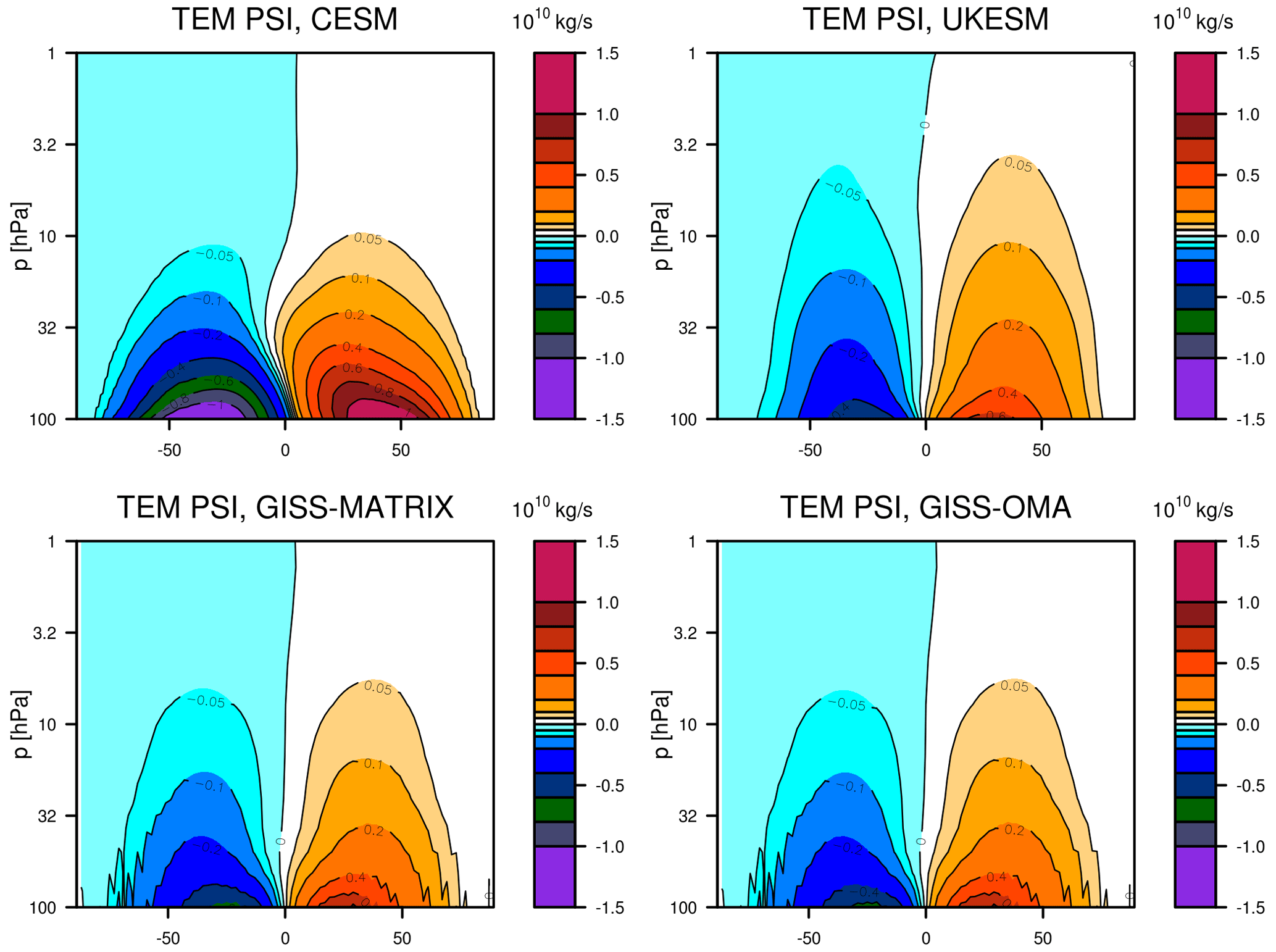
Figure 2Climatological mass streamfunction of the residual circulation averaged over 2035–2064 in the control SSP2–4.5 for each of the four models.
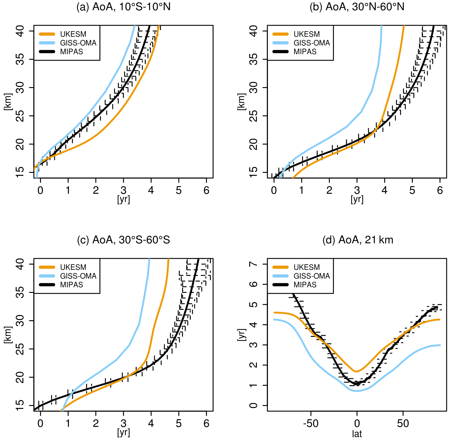
Figure 3Normalized age of air (AoA; years) at (a) 10∘ S–10∘ N, (b) 30∘ S–60∘ N, (c) 30∘ N–60∘ S, and (d) 21 km diagnosed from the UKESM (orange) and GISS-OMA (light blue) CMIP6 historical integration. Note that the GISS-OMA simulation uses prescribed sea surface temperatures (SSTs) and sea ice (unlike the SAI GISS-OMA simulations, which include an interactive ocean module). Black lines show the corresponding AoA derived from the MIPAS SF6 satellite observations (black; Stiller et al., 2020). Both model and observed AoA values were averaged over the 7-year period from May 2005 to April 2012 inclusive. Both model and observed AoA values were normalized to be zero at the tropical tropopause by subtracting the values calculated in each case for the tropical tropopause layer (here approximated as a mean over 25∘ S–25∘ N, 16–17 km). CESM is not included as no AoA diagnostic is available from its historical CMIP6 simulations.
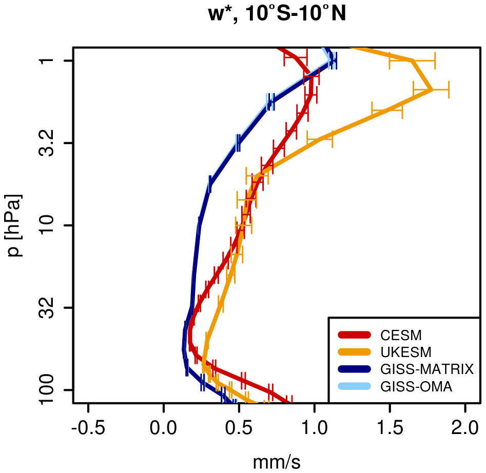
Figure 4Climatological transformed vertical residual velocity averaged over 2035–2064 and 10∘ S–10∘ N in the control SSP2–4.5 for each of the four models. Error bars denote ±2 standard error of the mean.
In the simulations with equatorial injections (third row in Fig. 1), the highest SAD values are found in the tropics, with the largest variability across the models in regions poleward of 30∘ latitude. UKESM shows the greatest confinement of sulfate inside the tropical pipe out of the different models; the stronger confinement in UKESM is also visible for other injection locations. Comparison of the UKESM age of air (AoA) with MIPAS satellite observations (Stiller et al., 2020) shows significantly older model AoA in the tropics than observed (Fig. 3); this indicates a slow rate of transport out of the tropics and is thus consistent with the high fraction of sulfate aerosols found at low latitudes. In addition, UKESM simulates the fastest vertical velocities in the tropics at the altitudes where sulfate aerosols are injected (∼22 km, Fig. 4). This slows down the gravitational settling of aerosols, thereby adding to their tropical confinement. The effect is further amplified by the relatively smaller aerosol sizes in UKESM than in CESM2 (as indicated by the locally higher SAD in Fig. 1; see also Fig. 5 in Part 1), with a maximum effective radius of ∼0.3 µm in UKESM compared to ∼0.6 µm in CESM2.
Both GISS-MATRIX and GISS-OMA show a relatively deeper aerosol layer. This is partially because of the much smaller size of sulfate aerosols, resulting in slower gravitational settling and increased lifetime of sulfate aerosols in the stratosphere. As shown in Part 1, the maximum effective radius reaches ∼0.25 µm in GISS-MATRIX (compared to ∼0.6 µm in CESM2) but the value drops substantially near the injection location, corresponding to locally very small aerosol particles and very high SAD values (Fig. 1). The lack of an explicit aerosol nucleation model in CESM2, wherein nucleating aerosols are directly transferred to the Aitken mode, may help explain why such a drop is not present in CESM2 (see also Weisenstein et al., 2022). In addition, the GISS model shows anomalously young AoA throughout the depth of the tropical pipe when compared to observations (Fig. 3) but relatively slow resolved upwelling (Fig. 4), thus suggesting additional diffusion processes operating in the model that enhance transport of air (and aerosols) to higher altitudes by dispersion and/or mixing.
Importantly, GISS-OMA shows substantially (i.e., a few times) larger sulfate SAD than any other models with two-moment aerosol microphysics (Fig. 1, rightmost column). The bulk aerosol scheme restricts the mean size of aerosols (with the imposed dry radius of 0.15 µm), thereby preventing their growth by coagulation and leading to the formation of a large number of relatively small aerosols. These high sulfate concentrations are also readily transported to higher latitudes since smaller particles have lower gravitational settling velocities and increased atmospheric lifetimes. In addition, horizontal mixing in GISS is likely very strong – this can be inferred from the anomalously young model AoA simulated throughout the stratosphere (Fig. 31). In general, AoA shows combined effects of transport from the residual circulation and mixing (Garny et al., 2014). Since the residual circulation simulated in the two GISS models is generally comparable to that in UKESM and much weaker than in CESM2 (Fig. 2), the relatively younger AoA in GISS is mostly likely the result of much stronger mixing. This is further supported by the weaker climatological zonal winds simulated in GISS in the stratosphere in both hemispheres (Fig. S2) and thus weaker potential vorticity gradients that control mixing efficiency (Abalos and de la Cámara, 2020). Neither of the two GISS models is able to simulate the Quasi-Biennial Oscillation (QBO; see also Sect. 3.5), which is known to be an important factor in controlling the confinement of aerosols inside the tropical latitudes (Niemeier and Schmidt, 2017; Visioni et al., 2018).

Figure 5Shading: yearly mean changes in temperature [K] averaged over the last 8 years of the simulations compared to the same period in the SSP2–4.5 run for CESM (column 1), UKESM (column 2), GISS-MATRIX (column 3), and GISS-OMA (column 4). Contours show the values in the control SSP2–4.5 run for reference. Stippling as in Fig. 1.
3.2 Temperature
The absorption of incoming solar and outgoing terrestrial radiation by sulfate aerosols increases temperatures in the tropical lower stratosphere in the three models with two-moment aerosol microphysics (Fig. 5). These changes in stratospheric temperatures, whilst far away from the surface, can drive a dynamical response (Sect. 3.3 and 3.5) that alters stratospheric composition (Sect. 3.3 and 3.4) and indirectly affects regional surface climate (Part 1). In these simulations, while lower stratospheric temperatures increase primarily in the tropics, both CESM2 and GISS-MATRIX also show substantial temperature increases in the midlatitude lower stratosphere in the hemisphere of injection. This is consistent with both models showing significant aerosol levels outside the tropics (Sect. 3.1, Fig. 1; see also Part 1). In each model, the tropical lower stratospheric warming is strongest for the equatorial injection case (Fig. 5; e.g., up to ∼4–6 K for off-equatorial injections and up to ∼8 K for the equatorial injection in CESM2).
The magnitude of the lower stratospheric warming is approximately a factor of 2 smaller in UKESM than in CESM2. This can be partially understood by the smaller average size of sulfate aerosols (as can be inferred from SAD values in Fig. 1, see also Part 1), which are less effective at absorbing terrestrial radiation (Laakso et al., 2022), and by the smaller total sulfate aerosol load (Part 1). However, differences in the radiative codes are likely still an important contributing factor (e.g., Boucher et al., 1998; DeAngelis et al., 2015; Niemeier et al., 2020). For the equatorial injection case in UKESM, the strong confinement of sulfate aerosols inside the tropical pipe, as well as their uplift via the somewhat faster tropical velocities (Fig. 3), leads to a greater vertical extent of the lower stratospheric warming.
In GISS-MATRIX, the lower-stratospheric warming is comparable to CESM2 in terms of the maximum amplitude but much more vertically spread for all injection locations. As discussed in Sect. 3.1, this is related to a greater depth of the aerosol layer in GISS-MATRIX, resulting from smaller sulfate particle sizes and thus slower gravitational settling, a weaker shallow branch of the BDC, and likely stronger diffusion. In addition, the associated acceleration of tropical upwelling in the stratosphere from aerosol heating, which acts to increase adiabatic cooling and thus opposes the diabatic heating from aerosol absorption, is much smaller in GISS-MATRIX than in CESM2 (Fig. 6).
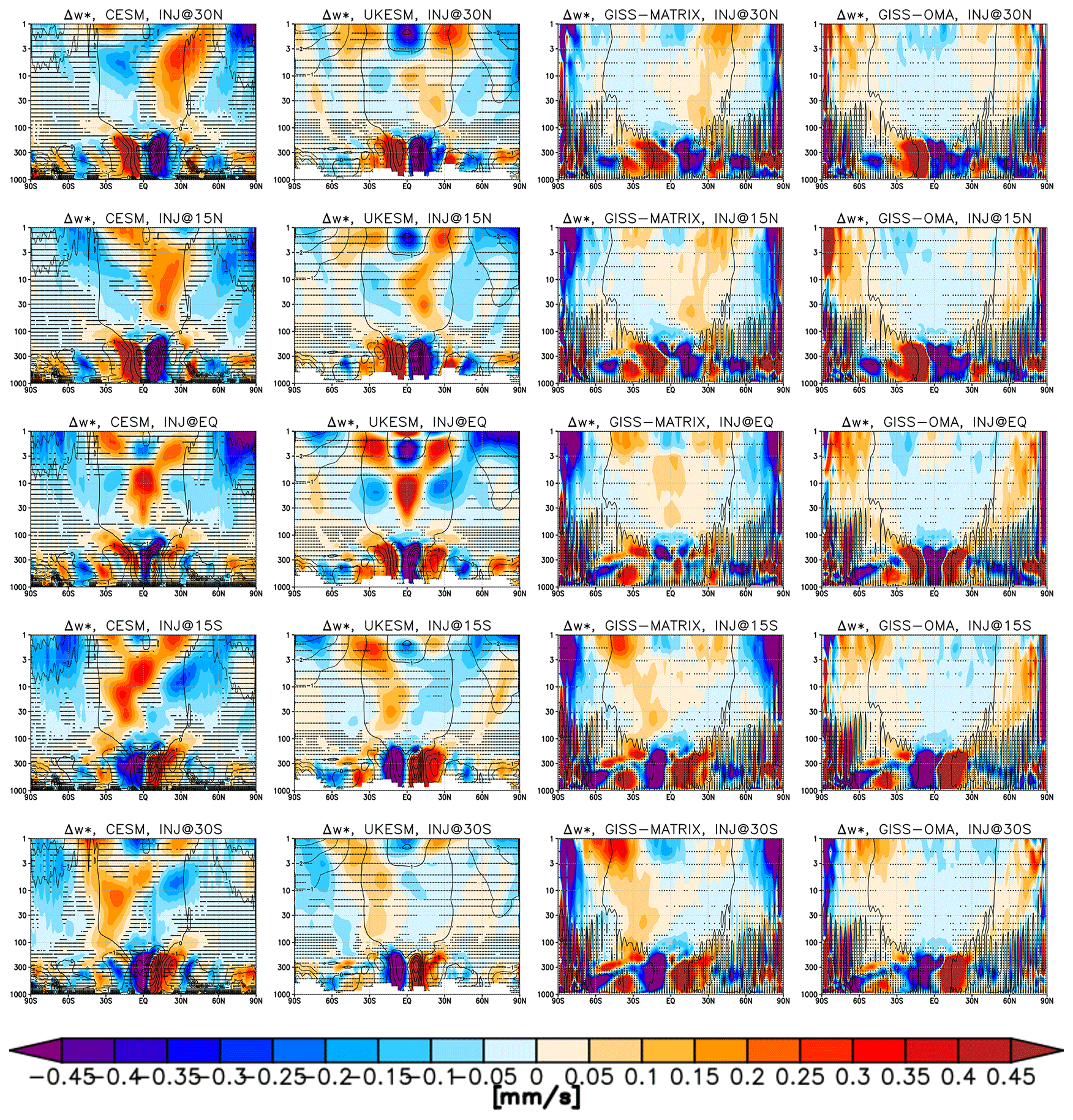
Figure 6Shading: yearly mean changes in transformed vertical velocity [mm s−1] averaged over the last 8 years of the simulations compared to the same period in the SSP2–4.5 run for CESM (column 1), UKESM (column 2), GISS-MATRIX (column 3), and GISS-OMA (column 4). Positive values indicate anomalous upwelling. Contours show the vertical velocities in the control SSP2–4.5 run for reference (note that for GISS-MATRIX and GISS-OMA only the 0 contour is plotted for clarity). Stippling as in Fig. 1.
In contrast to the three models with two-moment microphysics, no lower-stratospheric warming is simulated in GISS-OMA (Fig. 5, rightmost column). The use of a bulk aerosol scheme with fixed aerosol sizes results in much smaller particles than for the models with more complex aerosol schemes; the small aerosols are not as effective in absorbing radiation. In addition, the simulations are associated with substantial reductions in lower-stratospheric ozone (Sect. 3.3), which otherwise contributes to the shortwave heating there (Richter et al., 2017); these thus effectively offset any warming tendency from aerosol absorption.
As expected, all models simulate tropospheric cooling as a result of the reduction of the incoming solar radiation from SAI. In each model, the strongest cooling is found in the hemisphere of injection, consistent with the near-surface temperature changes discussed in Part 1. In each case the cooling maximizes in the tropical upper troposphere; this is consistent with changes produced by the strong radiative feedback from water vapor, the tropospheric concentrations of which decrease when the surface is cooled (Sect. 3.4). As the result, surface temperature signals tend to be amplified in the upper troposphere; this is also the case under global warming from rising greenhouse gases (Sherwood et al., 2010; Steiner et al., 2020) and predicted by the moist adiabatic lapse rate theory (Stone and Carlson, 1979). However, here the magnitude of the tropospheric cooling varies substantially between the models, with the two GISS models showing the strongest responses, consistent with the near-surface temperature changes discussed in Part 1. A large difference in the upper tropospheric temperature responses amongst models has also been observed under climate change simulations (Minschwaner et al., 2006).
3.3 Ozone and large-scale circulation
3.3.1 Stratospheric ozone changes in models with two-moment microphysics
Changes in tropospheric and stratospheric temperatures, and hence the large-scale transport as a result of SAI, drive changes in stratospheric ozone. The absorption of incoming solar radiation by stratospheric ozone plays a crucial role in shielding the Earth's surface from harmful UV radiation, thus having direct impacts on human health and ecosystems. In addition, the absorption of outgoing terrestrial radiation by ozone in the troposphere and lower stratosphere contributes to the greenhouse effect. Therefore, any ozone changes there can modulate the direct radiative response from aerosol reflection, impacting the surface temperature responses discussed in Part 1.

Figure 7Shading: yearly mean changes in ozone [%] averaged over the last 8 years of the simulations compared to the same period in the SSP2–4.5 run for CESM (column 1), UKESM (column 2), GISS-MATRIX (column 3), and GISS-OMA (column 4). Contours show the ozone mixing ratios [ppmv] in the control SSP2–4.5 run for reference. Stippling as in Fig. 1.
CESM2, UKESM, and GISS-MATRIX all show increased ozone in the tropical lower stratosphere at ∼70 hPa (Fig. 7). The response results from local deceleration of upwelling in the tropical troposphere (Fig. 6) brought about by the increase in static stability associated with heating in the lower stratosphere and cooling in the troposphere (Fig. 5). This deceleration of tropospheric upwelling slows down the transport of ozone-poor tropospheric air into the lower stratosphere, thus increasing ozone in the region. The deceleration of tropical upwelling also reduces precipitation (e.g., Simpson et al., 2019), thereby further modulating the precipitation responses discussed in Part 1. For ozone, the differences in the magnitudes of ozone responses amongst the three models with two-moment aerosol microphysics are commensurate with the differences in the lower-stratospheric temperature responses, with larger ozone increases in GISS-MATRIX and CESM2 and smaller in UKESM. We find a strong correlation between the lower-stratospheric ozone and temperature responses across the models (Fig. 8). This demonstrates that whilst differences remain in the magnitudes of these responses amongst different models, such uncertainties are coherently correlated within each model.
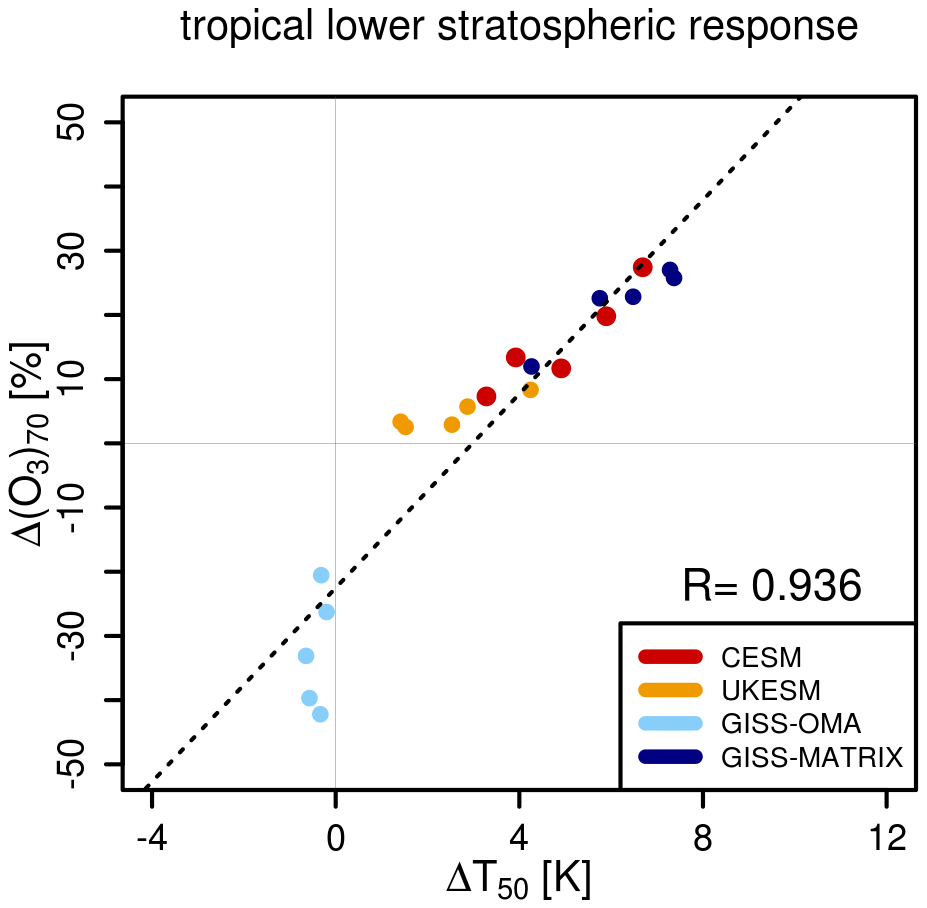
Figure 8Correlation between yearly mean 30∘ S–30∘ N changes in temperature at 50 hPa and ozone at 70 hPa between each of the SAI experiments and SSP2–4.5. Colors indicate the models, and the dashed black line shows a linear fit to all results for the four models together.
In the middle stratosphere, CESM2, UKESM, and GISS-MATRIX all show local ozone reductions near the latitude of SAI, as well as further ozone increases higher up (CESM and UKESM only). These changes can also be explained by the associated changes in the large-scale residual circulation, which redistributes ozone to and from its photochemical production region (i.e., tropical middle stratosphere, where ozone mixing ratios maximize). The acceleration of tropical upwelling in the stratosphere near the latitude of injection brings more air with lower ozone mixing ratios from the lower to middle stratosphere (and, conversely, more air with higher ozone mixing ratios from the middle to upper stratosphere). Note that although the simulated tropical and midlatitude ozone responses are primarily dynamically driven (by changes in ozone transport), any associated changes in chemistry (Tilmes et al., 2018b, 2021) do contribute to the simulated responses (Tilmes et al., 2022). In contrast to CESM2 and UKESM, GISS-MATRIX shows a small ozone decrease of a few percent in the upper stratosphere; the response is consistent with the elevated ClO in the region (Fig. S3) and suggests problems in the chemistry scheme in GISS that merit further attention by the modeling teams.
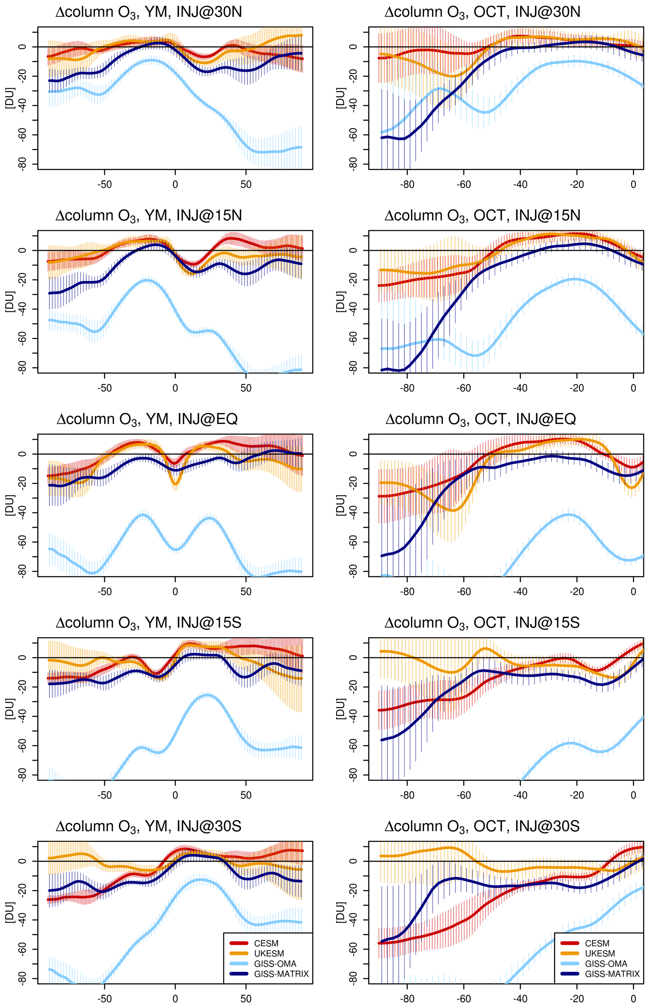
Figure 9Yearly mean (YM; left) and October mean (OCT; right) changes in total column ozone [DU] averaged over the last 8 years of the simulations compared to the same period in the SSP2–4.5 run for CESM (red), UKESM (orange), GISS-MATRIX (dark blue), and GISS-OMA (light blue). Error bars indicate ±2 standard errors of the difference in means.
When ozone responses are integrated vertically over the whole atmosphere (Fig. 9), we find reasonably good agreement between the tropical column ozone responses between CESM2 and UKESM. Both models show local decreases in column ozone near the injection latitude of the order of ∼10 DU and small but statistically significant increases in tropical ozone columns of a few DU further away. In general, these tropical ozone changes, whilst small in absolute terms, can play a relatively important role given the much lower climatological column ozone values found in the tropics than at higher latitudes. A similar pattern of tropical column O3 responses was also found in GISS-MATRIX, although the column O3 changes there tend to be more negative, presumably because of the contribution of the reductions in upper-stratospheric ozone (the origins of which in this model, as discussed above, are not fully understood and suggest problems in the chemistry scheme).
3.3.2 Antarctic stratosphere
Previous decades have seen significant reductions of ozone in the Southern Hemisphere (SH) high latitudes brought about by accelerated heterogenous halogen reactions inside the Antarctic polar vortex as a result of anthropogenic emissions of ozone-depleting substances. Therefore, future evolution and recovery of Antarctic ozone continue to be the focus of significant scientific and political interest (WMO, 2018). CESM2 shows a significant ozone decrease in the lower stratosphere as a result of SAI, in particular for the SH injections (up to ∼35 % ozone decrease in the polar lowermost stratosphere, Fig. 7, or up to ∼50 DU vertically averaged, Fig. 9). These yearly mean changes are dominated by the response during austral spring (Figs. S5 and 9), i.e., when the impact of heterogenous halogen activation on polar ozone maximizes. As discussed in Sect. 3.1, CESM2 has a very fast shallow BDC, which effectively transports sulfate aerosols from the SO2 injection locations in the tropics to higher latitudes. The presence of increased surface area densities in polar regions (Fig. 1) facilitates heterogenous halogen reactions inside the cold polar vortex that convert halogen species from their reservoir forms into active species like ClO or BrO (Figs. S4 and S5); these then enhance catalytic ozone destruction during austral spring.
A similar decrease in the SH lower stratospheric ozone is not reproduced in UKESM in the yearly mean (Fig. 7). The model also does not show any significant Antarctic ozone depletion during austral spring (Figs. 9 and S5). First, UKESM shows greater confinement of sulfate aerosols inside the tropical pipe and weaker shallow BDC than CESM2 (Sect. 3.1). Therefore, the model simulates much lower aerosol concentrations at high latitudes (Fig. 1). Second, UKESM does not include the important heterogenous ClONO2 + HCl reaction on sulfate aerosols or any heterogenous bromine chemistry on sulfate aerosols. Both effects significantly reduce the concentrations of activated halogens simulated in the lower stratosphere under SAI (Figs. S3 and S4), which thus limits the amount of catalytic ozone depletion in the Antarctic lower stratosphere.
We note that, in general, the magnitude of the chemical ozone response depends on the background stratospheric halogen concentrations, which are projected to decrease over the 21st century, and thus any halogen-catalyzed ozone reduction from SAI would be lower in later parts of the century (Tilmes et al., 2021). Similar considerations will also apply to the impacts of SAI on the Arctic ozone; however, the short length of the simulations (i.e., 8 years analyzed) does not allow us to assess this confidently, as any changes in ozone in the NH high latitudes will be dominated by natural interannual variability.
In comparison, the two-moment version of GISS also show decreases in Antarctic ozone in the lower stratosphere coinciding with local increases in ClO (Fig. S3). However, the coupled O3–ClO response is qualitatively and quantitatively similar for all injection cases (despite large differences in the high-latitude sulfate levels), suggesting that factors other than the latitudinal distribution of sulfate and thus of anomalous heterogenous halogen activation on aerosol surfaces could be an important but erroneous contributing driver in the model.
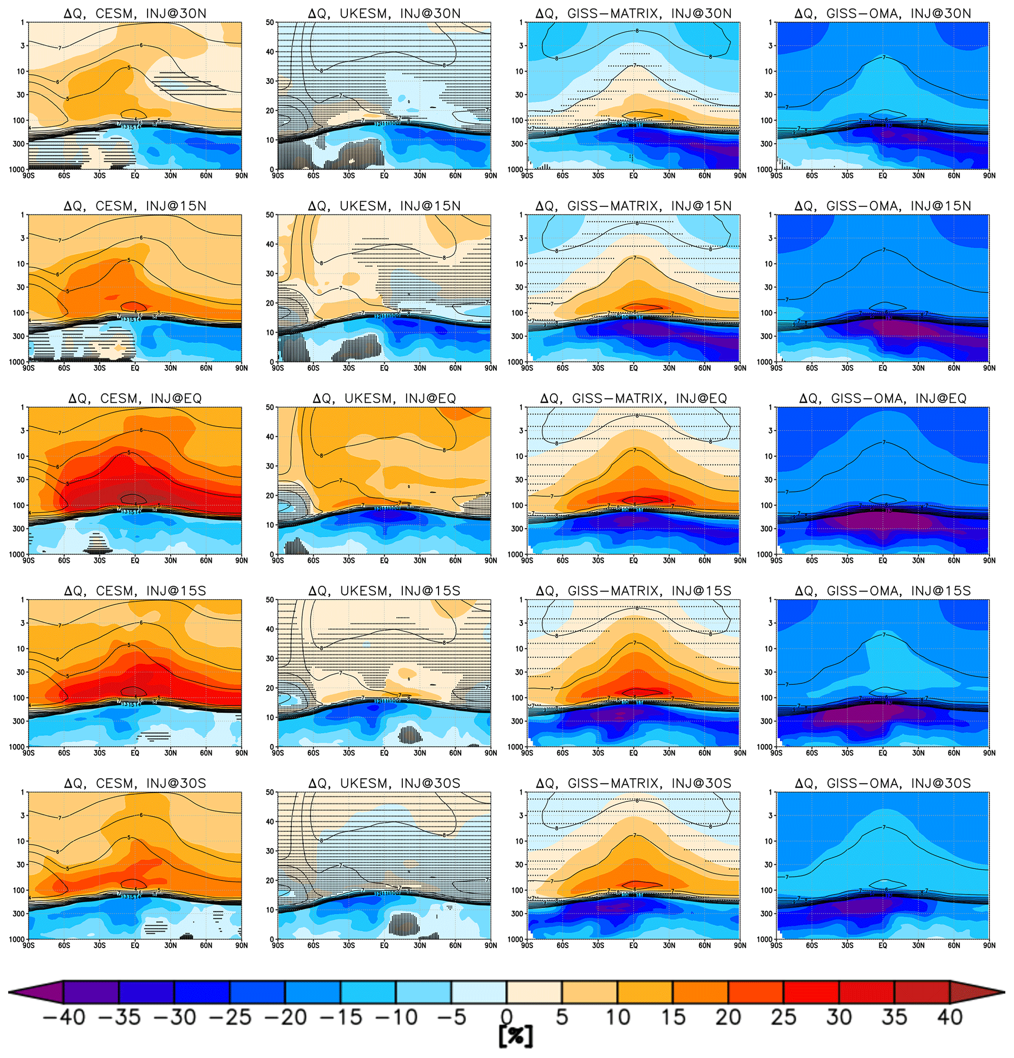
Figure 10Yearly mean changes in specific humidity [%] averaged over the last 8 years of the simulations compared to the same period in the SSP2–4.5 run for CESM (column 1), UKESM (column 2), GISS-MATRIX (column 3), and GISS-OMA (column 4). Contours indicate the corresponding values in the SSP2–4.5 experiment in the units of parts per million by volume (ppmv) for reference. Stippling as in Fig. 1.
3.3.3 Tropospheric ozone changes
In addition to acting as a greenhouse gas, in the troposphere ozone constitutes an atmospheric pollutant, adversely impacting human health (e.g., Eastham et al., 2018), crop production (e.g., Xia et al., 2017), and ecosystems (e.g., Zarnetske et al., 2021). Here we find significant reductions of tropospheric ozone (up to ∼15 %) in GISS-MATRIX throughout most of the troposphere. The response is likely related to the significantly stronger tropospheric cooling (Fig. 5) and thus a stronger reduction in tropospheric water vapor (Fig. 10), which plays an important role in the tropospheric ozone budget. The reduction in tropospheric ozone in the tropics is not reproduced in either CESM2 or UKESM, likely because of the smaller level of tropospheric cooling in these models. In addition, the CESM2 version used includes a chemistry scheme tailored for middle atmosphere studies and thus does not include comprehensive tropospheric chemistry; this factor thus likely played a role in determining the tropospheric ozone response simulated in the model. The CESM2 model does, however, show significant reductions in tropospheric ozone in the SH middle and high latitudes, in particular for the SH injections. The response is likely driven by the Antarctic lower-stratospheric ozone depletion (Sect. 3.3.2) and the resulting reduction in stratosphere-to-troposphere ozone transport (e.g., Xia et al., 2017).
3.3.4 Response in GISS model with bulk aerosol microphysics
In stark contrast to the ozone responses in the three models with more detailed aerosol microphysics, the bulk version of GISS simulates substantial reductions of lower stratospheric ozone throughout the globe (locally up to 40 %–60 %, Fig. 7). In the tropics, the GISS-OMA results constitute an outlier in the previously identified relationship between lower-stratospheric temperature and ozone responses (Fig. 8). The different ozone response in GISS-OMA is likely related to the number and size of sulfate aerosols produced from the SO2 injections, i.e., the very high concentrations of very small aerosols. Since smaller aerosols have proportionally larger surface areas than their larger counterparts, this leads to much higher sulfate SAD compared to the two-moment version of GISS (Fig. 1). In addition, smaller aerosols have longer lifetimes and can thus be transported rapidly by the presumed strong mixing in the model (Sect. 3.1). All of these factors lead to significantly elevated sulfate SAD simulated in GISS-OMA throughout the lower stratosphere. These could in principle enhance heterogenous halogen activation and thus explain the substantial ozone depletion found in these runs. We note, however, that the simulations do not show elevated active halogen concentrations in the lower stratosphere (the simulated lower-stratospheric ClO and BrOx levels in fact decrease under SAI in GISS-OMA, Figs. S3 and S4) but only spurious increases in ClO at higher altitudes, highlighting problems in the chemistry scheme in GISS that merit future attention.
3.4 Stratospheric water vapor
Figure 10 shows the associated changes in water vapor. As with ozone, the absorption of outgoing terrestrial radiation by water vapor in the lower stratosphere and the troposphere contributes to the greenhouse effect. Thus, any SAI-induced changes in it can further modulate the radiative balance and surface temperature responses discussed in Part 1. In addition, the photolysis of stratospheric water vapor (SWV) constitutes the main source of reactive HOx in the stratosphere, which acts to reduce stratospheric ozone levels and thereby further modulate the ozone responses discussed in Sect. 3.3.
We find large differences in the SWV responses amongst the models, ranging from +40 % to −15 % in the tropical lower stratosphere for the equatorial injections. SWV increases in CESM2 and GISS-MATRIX for all injection locations, consistent with the increase in cold-point tropopause temperatures associated with the warming of the tropical lower stratosphere. The increase in SWV is strongest in the simulations with equatorial injections (up to 40 % and 25 % in the tropical lower stratosphere for CESM2 and GISS-MATRIX, respectively), consistent with the strongest lower-stratospheric warming (Sect. 3.2, Fig. 5). However, while the increase in SWV in CESM2 is simulated throughout the entire stratosphere, the GISS-MATRIX simulations show negative SWV changes in the upper stratosphere, especially at high latitudes; the latter may be related to its problems with halogen chemistry there (see Sect. 3.3).
The significant increase in SWV under SAI is not reproduced in UKESM, which does not show substantial changes in SWV in any of the experiments except for the equatorial injection (up to 15 % in the tropical lower stratosphere). In fact, instead of an increase in SWV seen in CESM2 and GISS-MATRIX, there is a very small decrease in SWV for simulations with injections at 30∘ S and 30∘ N. This may be related to anomalously high climatological SWV in that model (Archibald et al., 2020). The increase in SWV under SAI is also not reproduced in GISS-OMA, which shows decreases in SWV (up to % in the high-latitude upper stratosphere) consistent with the absence of warming in the lower stratosphere, similar to the GISS response reported in Pitari et al. (2014). Nonetheless, in all simulations carried out with the four models water vapor decreases in the troposphere as a result of surface and tropospheric cooling, with the largest changes found for GISS-OMA.
We note that apart from the differences in the SAI responses amongst the models, we also find large differences in the climatological SWV values (contours in Fig. 10). These differences are consistent with the large inter-model spread in SWV reported amongst all CMIP6 models (Keeble et al., 2021).
3.5 Zonal winds
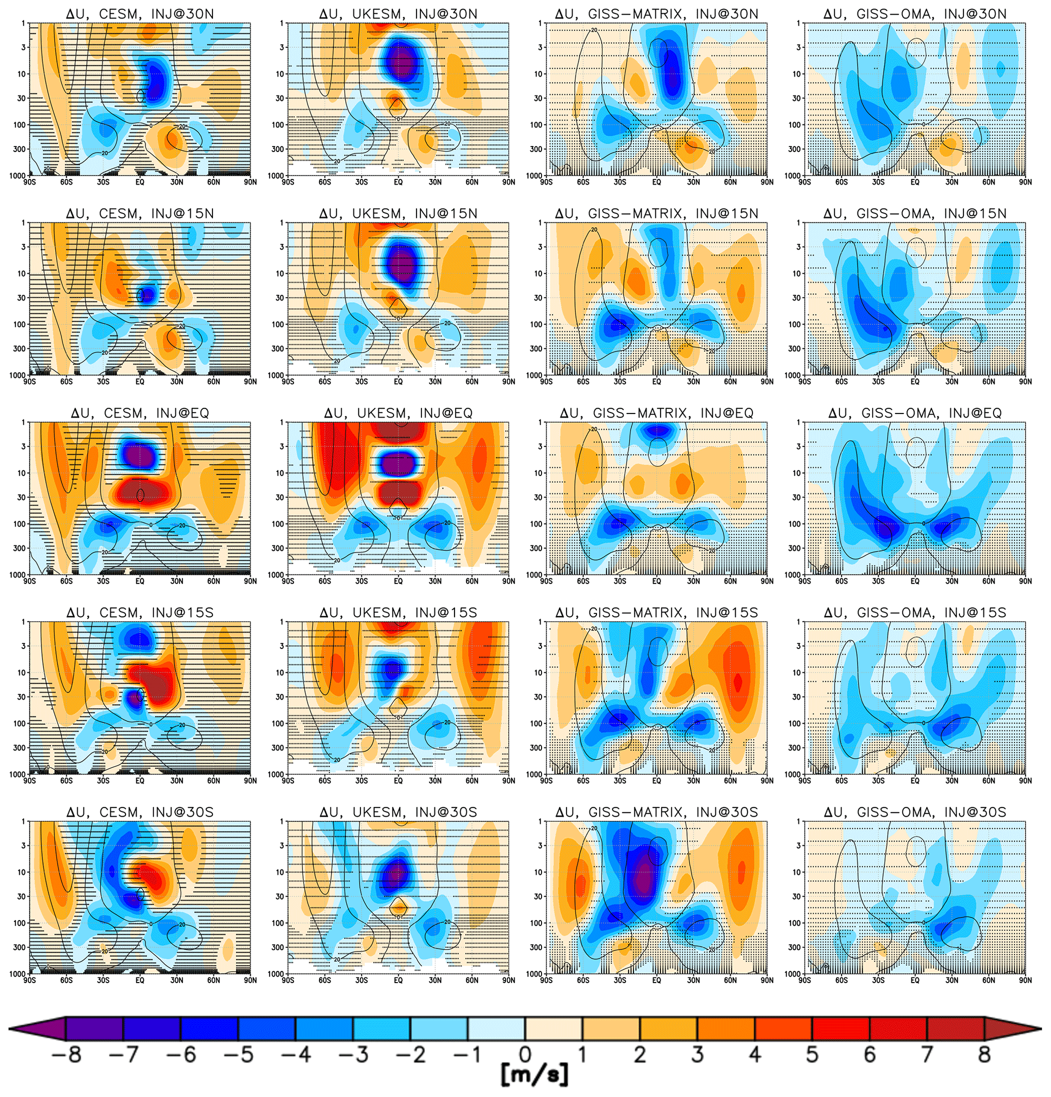
Figure 11 shows changes in zonal winds resulting from SAI. Note that both CESM2 and UKESM include an internally generated QBO, whilst the two GISS versions do not. The equatorial SO2 injection in CESM2 and UKESM leads to a westerly response in the tropical lower stratosphere and an easterly response above. This pattern corresponds to a locking of the QBO in a permanent westerly phase (Fig. S6; see also, e.g., Aquila et al., 2014; Jones et al., 2022) and arises because of the acceleration of equatorial upwelling under SAI (Fig. 6), inhibiting the downward propagation of the westerly QBO shear (Franke et al., 2021). A similar response was also found for UKESM in the G6 GeoMIP experiment (Jones et al., 2022). In general, the variability in equatorial zonal winds has been linked to variability in tropical tropospheric convection, subtropical and midlatitude tropospheric jets, and modes of high-latitude variability, e.g., the North Atlantic Oscillation (Anstey et al., 2022). Therefore, any SAI impacts on the QBO, including its locking in a permanent westerly phase under equatorial injections, have potential to impact the circulation in regions outside the equatorial stratosphere, although longer simulations would be needed to confidently diagnose such teleconnections. In any case, the QBO locking is not reproduced for the 15 and 30∘ injections in CESM2 and UKESM (Fig. S6); this is because the acceleration of tropical upwelling occurs off-equatorial near the injection latitudes (Fig. 6). The results illustrate that off-equatorial injections successfully avoid QBO locking, in agreement with Kravitz et al. (2019). Since the two GISS models do not include any representation of the QBO, the zonal wind is always easterly in the entire tropical stratosphere (Fig. S6).
In the extratropical stratosphere, CESM2, UKESM, and GISS-MATRIX all simulate strengthening of stratospheric jets in both hemispheres, consistent with geostrophic balance and the strengthening of the horizontal temperature gradient brought about from heating in the lower stratosphere. The results suggest impacts on the modes of high-latitude variability, including the Northern Annular Mode and Southern Annular Mode (NAM and SAM, respectively), which would influence regional middle- and high-latitude surface temperature and precipitation patterns during dynamically active seasons (e.g., boreal winter in the NH). However, here the derived responses are substantially affected by interannual variability due to the short length of the integrations; this prevents confident analysis of any inter-model differences or the dependence of the stratospheric polar vortex response on the latitude of injection. Unlike the three models with two-moment microphysics, GISS-OMA shows weakening of zonal winds in the lower stratosphere and the free troposphere below, consistent with the tropical tropospheric cooling simulated in the model.
In the troposphere, however, i.e., where the interannual variability is lower, all models suggest qualitatively consistent impacts on the tropospheric jets, which are important for modulating midlatitude weather patterns. In particular, the off-equatorial injection cases show an equatorward shift of the tropospheric jet in the hemisphere of injection and an opposite sign response in the other hemisphere. In the case of equatorial injections, tropospheric jets weaken in both hemispheres. The qualitative agreement between GISS-OMA, which does not show a warming in the tropical lower stratosphere, and the other three models illustrates the role of changes in meridional temperature gradients within the troposphere for the simulated changes in tropospheric jets.
This paper constitutes Part 2 of the study performing a first systematic inter-model comparison of atmospheric responses to equatorial and off-equatorial stratospheric SO2 injections. We used three comprehensive Earth system models – CESM2-WACCM6, UKESM1.0, and GISS-E2.1-G. For the latter we used two model versions, one with two-moment and one with bulk aerosol microphysics, to illustrate the importance of a detailed treatment of aerosol processes. We performed a set of five sensitivity experiments with constant point injections of 12 Tg SO2 yr−1 in the lower stratosphere at either 30∘ S, 15∘ S, 0∘, 15∘ N, or 30∘ N.
Building on Part 1 of this study, we demonstrated how inter-model differences in the simulated sulfate aerosol fields relate to biases in the climatological circulation and specific aspects of the model microphysics. In particular, CESM2 was found to simulate larger concentrations of sulfate aerosols in the high latitudes than the other two models with two-moment microphysics. This could be understood in light of the significantly faster climatological shallow branch of the Brewer–Dobson circulation in CESM2, as well as a relatively isolated tropical pipe and older tropical age of air in UKESM. The two GISS versions also simulated elevated sulfate surface area densities at higher latitudes, consistent with smaller aerosol particles and relatively stronger horizontal mixing (thus very young stratospheric age of air).
We then characterized the simulated changes in stratospheric and free-tropospheric temperatures, ozone, water vapor, and large-scale circulation, elucidating the role of the above aspects in the surface SAI responses discussed in Part 1. A large spread in the magnitudes of the tropical lower-stratospheric warming was found amongst the models, and these could partially be attributed to the differences in aerosol distributions and their sizes. Whilst differences in radiative parameterizations certainly also played an important role, those are harder to isolate and would require further sensitivity experiments (e.g., with fixed size distribution and specified chemistry). For each model, the strongest lower-stratospheric warming was found for the equatorial injection case, in agreement with previous studies (e.g., Kravitz et al., 2019). Regarding stratospheric ozone, all models with two-moment aerosol microphysics agreed in the tropical and subtropical regions and suggested local decreases in total column ozone of ∼10 DU near the latitude of injection as well as small increases in the tropical–subtropical regions further away. The ozone responses there could be explained by the associated changes in upwelling and the large-scale Brewer–Dobson circulation and were thus commensurate in magnitude with the associated changes in lower-stratospheric temperatures amongst the models.
In contrast to the relative agreement amongst the models regarding ozone responses at low latitudes, we found a large inter-model spread in the Antarctic ozone responses; these could largely be explained by the differences in the simulated latitudinal distributions of sulfate noted above as well as the degree of implementation of heterogeneous halogen chemistry on sulfate amongst the models. In particular, CESM2 showed elevated surface area densities in the high latitudes; these facilitated heterogenous halogen reactions that accelerated catalytic springtime ozone destruction in the Antarctic stratosphere. A similar response was not simulated in UKESM, consistent with a stronger confinement of sulfate aerosols inside the tropical pipe as well as an incomplete treatment of heterogenous halogen chemistry on sulfate in the model version used.
For stratospheric water vapor, the study found substantial spread of the model responses to sulfate injections, ranging from −15 % to +40 % in the tropical lower stratosphere. CESM2 and GISS-MATRIX both showed significant increases in stratospheric water vapor consistent with the increases in the tropical cold-point temperatures. The response was not reproduced in UKESM, which only showed a substantial (up to ∼15 %) increase in stratospheric water vapor in the equatorial injection case, or in GISS-OMA, wherein stratospheric water vapor decreased as a result of the absence of lower stratospheric warming.
In general, the sensitivity simulations with GISS using simple bulk aerosol microphysics illustrate the importance of a more detailed treatment of aerosol processes. In particular, the simulations showed very high sulfate surface area densities as a result of the very small aerosol sizes; these were in turn associated with changes in stratospheric ozone (including substantial reductions in the lower stratosphere of up to ∼40 %–60 %), temperatures, water vapor, and zonal winds that contrasted strongly with the models using two-moment aerosol microphysics. While problems in the halogen chemistry were identified in GISS that require further assessment by the modeling teams, the results point towards the importance of detailed treatment of aerosol microphysics, including resolving the complex relationships between the size distributions of aerosols and their physical and chemical properties, for accurate modeling of climate impacts from SAI. The importance of a detailed treatment of aerosol microphysics for the simulated SAI responses was also recently highlighted by Laakso et al. (2022), wherein multiple injection scenarios were simulated with the same model using two different microphysical schemes (in this case a modal and a sectional scheme); the resulting differences in simulated aerosol size distributions led to varying estimates of the overall radiative forcing produced by SAI.
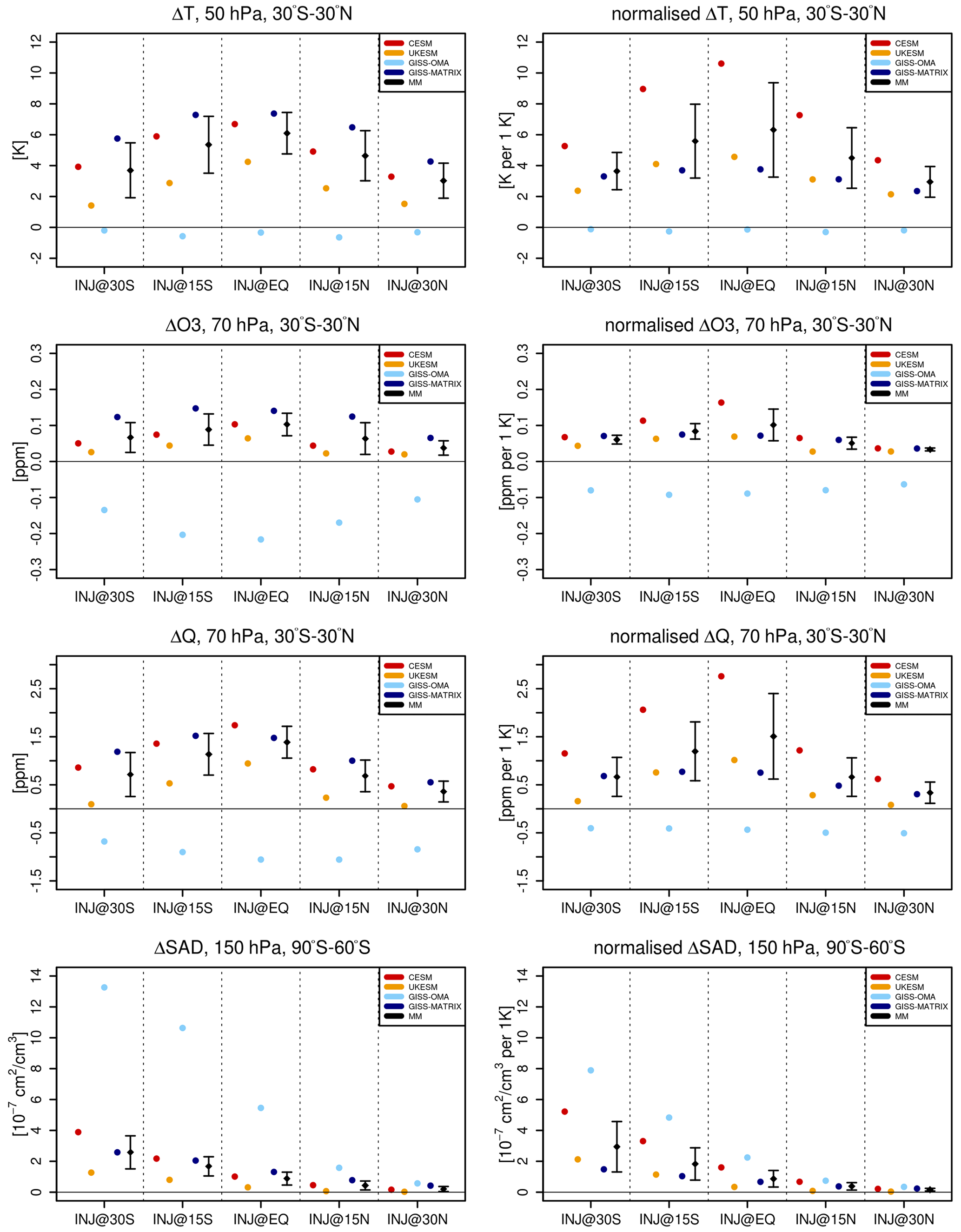
Figure 12Yearly mean stratospheric responses simulated in each model in each simulation expressed as (left) absolute changes and (right) changes normalized with the corresponding global mean surface temperature decrease. Rows top to bottom are for changes in tropical temperature at 50 hPa, tropical ozone at 70 hPa, tropical water vapor at 70 hPa, and Antarctic sulfate surface area densities at 150 hPa. Black points and whiskers denote multi-model means of CESM2, UKESM, and GISS-MATRIX responses ±1 standard deviation.
We summarize the results of this work in Fig. 12, where we offer an overview of relevant stratospheric changes due to SAI in two ways: in terms of both absolute responses (left panels) and responses normalized by the associated global mean changes in surface temperature (right panels) for each experiment and model (similar to what is done in Part 1). Black points and whiskers show the corresponding multi-model responses (note that GISS-OMA results are excluded from the multi-model means). This allows us to highlight some novel and interesting features.
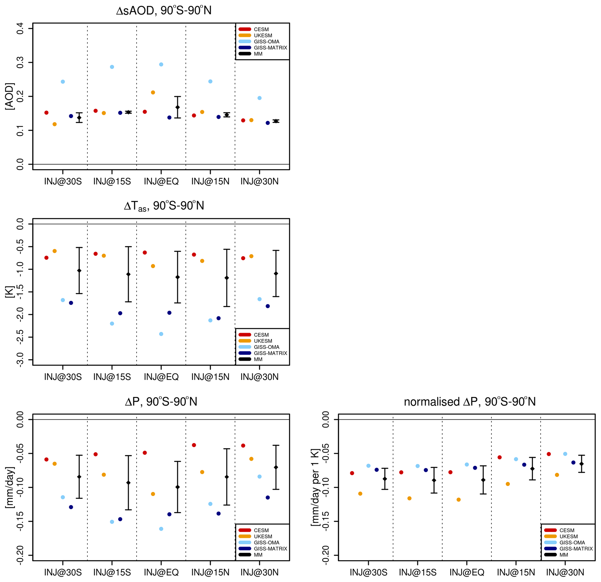
Figure 13As in Fig. 12 but for changes in global mean (top to bottom): stratospheric aerosol optical depth (AOD), surface temperature, and precipitation.
We find that the inter-model uncertainty in the absolute stratospheric responses increases under off-equatorial injections compared to the equatorial ones. This is in contrast to what one would expect based on the uncertainty in AOD, which is largely driven by aerosol microphysical properties and thus maximizes under equatorial injections (Fig. 13a); in that case, a strong confinement of the aerosol cloud results in much larger differences in the aerosol size distribution (Part 1, see also Visioni et al., 2018). In the stratosphere, however, uncertainties are also significantly affected by other drivers that, moreover, change depending on the injection location. For equatorial injections, the main source of uncertainty is the differences in tropical dynamics (and its interplay with aerosol microphysics). For 15∘ injections, uncertainties are larger because models disagree over the strength and location of the tropical pipe edges. In that case, UKESM results are characterized by the relatively large confinement of the simulated aerosol cloud inside the tropical pipe, resulting in a different response compared to models for which 15∘ lies outside it. Finally, for 30∘ injections uncertainties are driven mainly by differences in isentropic mixing and the large-scale poleward transport.
In contrast, if the inter-model uncertainties are considered in terms of the responses normalized with the associated global mean surface cooling, the picture changes and the largest inter-model spread is observed for the equatorial injections (right panels in Fig. 12). Overall, Fig. 12 highlights the fact that determining how SAI-related uncertainties change with changing injection location strongly depends on how these uncertainties are defined; this is especially true if the efficacy of the produced global cooling is considered the most relevant parameter and all other changes are defined per a unit of it.
Our findings illustrate the importance of a detailed and adequate representation of a range of microphysical, dynamical, and chemical processes in models for accurately representing the potential impacts from SAI, both directly in the stratosphere and lower down at the surface. By demonstrating the role of biases in climatological circulation, our results highlight the importance of not only model microphysics but also transport processes for simulating the evolution of the aerosol plume. They also highlight the large uncertainties in the representation of these processes in current Earth system models and the need for realistic representation of both aspects for determining the aerosol response and thus the potential impacts of SAI on atmospheric radiative balance, composition, and circulation. This thus suggests that a certain degree of caution is needed in interpreting the results of studies conducted with single models and that more work should be undertaken to improve the models and evaluate them against the available observational data, e.g., from recent volcanic eruptions to evaluate the model aerosol microphysics or using long-lived tracers to evaluate model transport. For modeling intercomparisons, understanding and attributing the reasons behind the inter-model spread rather than focusing only on multi-model mean responses would help identify which model responses are likely more trustworthy and representative of the uncertainty in a hypothetical real-world SAI response and which arise from spurious model features or problems with the code. This in turn would help to identify the areas in need of potential future model development and thus to narrow the uncertainties in future model projections of SAI impacts. We have demonstrated here that our experiments provide a framework to assess model skills in simulating SAI response and attribute some of the sources of uncertainty and drivers of inter-model spread. As such, we would like to suggest them as a possible test-bed experiment for GeoMIP to assess model structural uncertainty, which would in turn help develop an intercomparison of more comprehensive SAI strategies.
The results underscore the dependence of the dynamical response to SAI on the latitude of SO2 injections. For example, CESM2 and UKESM both showed that off-equatorial injections avoid locking of the QBO in a perpetual westerly phase that was otherwise found for equatorial injection. In the troposphere, all models suggested qualitatively similar impacts on tropospheric jets, i.e., equatorward shift of the tropospheric jet in the hemisphere of injection and an opposite sign response in the other hemisphere. Given the short length of the simulations, detailed analysis of the dynamical response in both the stratosphere and the troposphere (e.g., impacts on the Northern and Southern Annular Modes) as well as its dependence on the latitude of SAI alongside the underlying mechanisms is beyond the scope of this study but will be explored in the future with longer simulations (and multiple ensemble members).
Finally, our results further confirm the need to think of potential SAI deployment considering multiple injection locations outside the Equator. Injecting SO2 at the Equator gives rise to the lowest efficiency of global cooling per AOD (Part 1) as a result of the confinement of sulfate inside the tropical pipe (thereby reducing the AOD global coverage; Part 1 and Sect. 3.1 here) as well as leading to the largest increases in lower-stratospheric temperatures (Sect. 3.2). The latter leads to the strongest increases in tropical lower-stratospheric water vapor (Sect. 3.4) and ozone (Sect. 3.3), which act to partially offset the direct aerosol-induced surface cooling and cause the strongest perturbations of stratospheric and tropospheric circulation (Sect. 3.3 and 3.5), thereby indirectly affecting the surface temperature and precipitation responses discussed in detail in Part 1 and summarized in Fig. 13 here. In a modeling framework, a feedback algorithm that adjusts injection rates annually to achieve some specified climate goals (e.g., global mean surface temperature and its interhemispheric and Equator-to-pole gradients, as in Kravitz et al., 2019; Tilmes et al., 2018a) would compensate for some of the differences in physical processes among the models (whether due to models not matching observations in some respect or due to “true” uncertainty), leading to more consistent large-scale surface climate outcomes (as also discussed in detail in Part 1). While this uncertainty compensation may be more representative of a hypothetical deployment of SAI, it would also confound diagnosis of the mechanisms underlying inter-model differences by creating a dependence between these underlying mechanisms and the amount and distribution of injection rates across latitudes (see Fasullo and Richter, 2022, for an example). Our fixed-injection-rate intercomparison thus constitutes an essential enabler to comparing simulations that incorporate such a feedback algorithm.
The output from model simulations is available at https://doi.org/10.7298/22cqmx33 (Visioni and Bednarz, 2022).
The supplement related to this article is available online at: https://doi.org/10.5194/acp-23-687-2023-supplement.
EMB performed the analysis and wrote the paper. DV performed the CESM simulations and helped with the discussion of the results and writing of the paper. BK performed the GISS simulations. AJ performed the UKESM simulations. All authors contributed to the discussion of the results and writing of the paper.
The contact author has declared that none of the authors has any competing interests.
Publisher's note: Copernicus Publications remains neutral with regard to jurisdictional claims in published maps and institutional affiliations.
This article is part of the special issue “Resolving uncertainties in solar geoengineering through multi-model and large-ensemble simulations (ACP/ESD inter-journal SI)”. It is not associated with a conference.
The Community Earth System Model (CESM) project is supported primarily by the National Science Foundation. We would like to acknowledge high-performance computing support from Cheyenne (https://doi.org/10.5065/D6RX99HX; Hart, 2017) provided by NCAR's Computational and Information Systems Laboratory, sponsored by the National Science Foundation. The UKESM simulations were carried out using MONSooN2, a collaborative high-performance computing facility funded by the Met Office and the Natural Environment Research Council.
Support for Ewa M. Bednarz, Daniele Visioni, and Douglas G. MacMartin was provided by the Atkinson Center for a Sustainable Future at Cornell University through SilverLining's Safe Climate Research Initiative and by the National Science Foundation through agreement CBET-2038246 for Douglas G. MacMartin. Support for Ben Kravitz was provided in part by the National Science Foundation through agreement CBET-1931641, the Indiana University Environmental Resilience Institute, and the Prepared for Environmental Change Grand Challenge initiative. Andy Jones and James M. Haywood were supported by the Met Office Hadley Centre Climate Programme funded by BEIS and by SilverLining through its Safe Climate Research Initiative. This material is based upon work supported by the National Center for Atmospheric Research, which is a major facility sponsored by the National Science Foundation under cooperative agreement no. 1852977.
The authors thank Alan Robock and two other anonymous reviewers for helpful comments that improved the paper.
This research has been supported by the Atkinson Center for a Sustainable Future at Cornell University through SilverLining's Safe Climate Research Initiative and by the National Science Foundation (grant nos. CBET-2038246 and CBET-1931641).
This paper was edited by Anja Schmidt and reviewed by Alan Robock and two anonymous referees.
Abalos, M. and de la Cámara, A.: Twenty-first century trends in mixing barriers and eddy transport in the lower stratosphere, Geophys. Res. Lett., 47, e2020GL089548, https://doi.org/10.1029/2020GL089548, 2020.
Anstey, J. A., Osprey, S. M. Alexander, J., Baldwin, M. P., Butchart, N., Gray, L. J., Kawatani, Y., Newman, P. A., and Richter, J. H.: Impacts, processes and projections of the quasi-biennial oscillation, Nat. Rev. Earth Environ., 3, 588–603, https://doi.org/10.1038/s43017-022-00323-7, 2022.
Aquila, V., Garfinkel, C., Newman, P., Oman, L., and Waugh, D.: Modifications of the quasi-biennial oscillation by a geoengineering perturbation of the stratospheric aerosol layer, Geophys. Res. Lett., 41, 1738–1744, 2014.
Archibald, A. T., O'Connor, F. M., Abraham, N. L., Archer-Nicholls, S., Chipperfield, M. P., Dalvi, M., Folberth, G. A., Dennison, F., Dhomse, S. S., Griffiths, P. T., Hardacre, C., Hewitt, A. J., Hill, R. S., Johnson, C. E., Keeble, J., Köhler, M. O., Morgenstern, O., Mulcahy, J. P., Ordóñez, C., Pope, R. J., Rumbold, S. T., Russo, M. R., Savage, N. H., Sellar, A., Stringer, M., Turnock, S. T., Wild, O., and Zeng, G.: Description and evaluation of the UKCA stratosphere–troposphere chemistry scheme (StratTrop vn 1.0) implemented in UKESM1, Geosci. Model Dev., 13, 1223–1266, https://doi.org/10.5194/gmd-13-1223-2020, 2020.
Bauer, S. E., Wright, D. L., Koch, D., Lewis, E. R., McGraw, R., Chang, L.-S., Schwartz, S. E., and Ruedy, R.: MATRIX (Multiconfiguration Aerosol TRacker of mIXing state): an aerosol microphysical module for global atmospheric models, Atmos. Chem. Phys., 8, 6003–6035, https://doi.org/10.5194/acp-8-6003-2008, 2008.
Bauer, S. E., Tsigaridis, K., Faluvegi, G., Kelley, M., Lo, K. K., Miller, R. L., Nazarenko, L., Schmidt, G. A., and Wu, J.: Historical (1850–2014) aerosol evolution and role on climate forcing using the GISS ModelE2.1 contribution to CMIP6, J. Adv. Model. Earth Sy., 12, e2019MS001978, https://doi.org/10.1029/2019MS001978, 2020.
Boucher, O., Schwartz, S. E., Ackerman, T. P., Anderson, T. L., Bergstrom, B., Bonnel, B., Chylek, P., Dahlback, A., Fouquart, Y., Fu, Q., Halthore, R. N., Haywood, J. M., Iversen, T., Kato, S., Kinne, S., Kirkevåg, A., Knapp, K. R., Lacis, A., Laszlo, I., Mishchenko, M. I., Nemesure, S., Ramaswamy, V., Roberts, D. L., Russell, P., Schlesinger, M. E., Stephens, G. L., Wagener, R., Wang, M., Wong, J., and Yang, F.: Intercomparison of models representing direct shortwave radiative forcing by sulfate aerosols, J. Geophys. Res., 103, 16979–16998, https://doi.org/10.1029/98JD00997, 1998.
Crutzen, P. J.: Albedo Enhancement by Stratospheric Sulfur Injections: A Contribution to Resolve a Policy Dilemma?, Clim. Change, 77, 211, https://doi.org/10.1007/s10584-006-9101-y, 2006.
Danabasoglu, G., Lamarque, J.-F., Bacmeister, J., Bailey, D. A., DuVivier, A. K., Edwards, J., Emmons, L. K., Fasullo, J., Garcia, R., Gettelman, A., Hannay, C., Holland, M. M., Large, W. G., Lauritzen, P. H., Lawrence, D. M., Lenaerts, J. T. M., Lindsay, K., Lipscomb, W. H., Mills, M. J., Neale, R., Oleson, K. W., Otto-Bliesner, B., Phillips, A. S., Sacks, W., Tilmes, S., van Kampenhout, L., Vertenstein, M., Bertini, A., Dennis, J., Deser, C., Fischer, C., Fox-Kemper, B., Kay, J. E., Kinnison, D., Kushner, P. J., Larson, V. E., Long, M. C., Mickelson, S., Moore, J. K., Nienhouse, E., Polvani, L., Rasch, P. J., and Strand, W. G.: The Community Earth System Model Version 2 (CESM2), J. Adv. Model. Earth Sy., 12, e2019MS001916, https://doi.org/10.1029/2019MS001916, 2020.
DeAngelis, A., Qu, X., Zelinka, M., and Hall, A.: An observational radiative constraint on hydrologic cycle intensification, Nature, 528, 249–253, https://doi.org/10.1038/nature15770, 2015.
Eastham, S., Weisenstein, D., Keith, D., and Barrett, S.: Quantifying the impact of sulfate geoengineering on mortality from air quality and UV-B exposure, Atmos. Environ., 187, 424–434, https://doi.org/10.1016/j.atmosenv.2018.05.047, 2018.
Fasullo, J. T. and Richter, J. H.: Scenario and Model Dependence of Strategic Solar Climate Intervention in CESM, EGUsphere [preprint], https://doi.org/10.5194/egusphere-2022-779, 2022.
Ferraro, A. J., Charlton-Perez, A. J., and Highwood, E. J.: Stratospheric dynamics and midlatitude jets under geoengineering with space mirrors and sulfate and titania aerosols, J. Geophys. Res.-Atmos., 120, 414–429, 2015.
Franke, H., Niemeier, U., and Visioni, D.: Differences in the quasi-biennial oscillation response to stratospheric aerosol modification depending on injection strategy and species, Atmos. Chem. Phys., 21, 8615–8635, https://doi.org/10.5194/acp-21-8615-2021, 2021.
Garny, H., Birner, T., Bonisch, H., and Bunzel, F.: The effects of mixing on age of air, J. Geophys. Res.-Atmos., 119, 7015–7034, https://doi.org/10.1002/2013jd021417, 2014.
Gettelman, A., Mills, M. J., Kinnison, D. E., Garcia, R. R., Smith, A. K., Marsh, D. R., Tilmes, S., Vitt, F., Bardeen, C. G., McInerny, J., Liu, H.-L., Solomon, S. C., Polvani, L. M., Emmons, L. K., Lamarque, J.-F., Richter, J. H., Glanville, A. S., Bacmeister, J. T., Phillips, A. S., Neale, R. B., Simpson, I. R., DuVivier, A. K., Hodzic, A., and Randel, W. J.: TheWhole Atmosphere Community ClimateModel Version 6 (WACCM6), J. Geophys. Res.-Atmos., 124, 12380–12403, https://doi.org/10.1029/2019JD030943, 2019.
Hart, D.: Cheyenne supercomputer, NCAR CISL Advanced Research Computing, https://doi.org/10.5065/D6RX99HX, 2017.
Jones, A., Haywood, J. M., Scaife, A. A., Boucher, O., Henry, M., Kravitz, B., Lurton, T., Nabat, P., Niemeier, U., Séférian, R., Tilmes, S., and Visioni, D.: The impact of stratospheric aerosol intervention on the North Atlantic and Quasi-Biennial Oscillations in the Geoengineering Model Intercomparison Project (GeoMIP) G6sulfur experiment, Atmos. Chem. Phys., 22, 2999–3016, https://doi.org/10.5194/acp-22-2999-2022, 2022.
Jones, A. C., Haywood, J. M., Dunstone, N., Emanuel, K., Hawcroft, M. K., Hodges, K. I., and Jones, A.: Impacts of hemispheric solar geoengineering on tropical cyclone frequency, Nat Commun., 8, 1382, https://doi.org/10.1038/s41467-017-01606-0, 2017.
Keeble, J., Hassler, B., Banerjee, A., Checa-Garcia, R., Chiodo, G., Davis, S., Eyring, V., Griffiths, P. T., Morgenstern, O., Nowack, P., Zeng, G., Zhang, J., Bodeker, G., Burrows, S., Cameron-Smith, P., Cugnet, D., Danek, C., Deushi, M., Horowitz, L. W., Kubin, A., Li, L., Lohmann, G., Michou, M., Mills, M. J., Nabat, P., Olivié, D., Park, S., Seland, Ø., Stoll, J., Wieners, K.-H., and Wu, T.: Evaluating stratospheric ozone and water vapour changes in CMIP6 models from 1850 to 2100, Atmos. Chem. Phys., 21, 5015–5061, https://doi.org/10.5194/acp-21-5015-2021, 2021.
Kelley, M., Schmidt, G. A., Nazarenko, L. S., Bauer, S. E., Ruedy, R., and Russell, G. L.: GISS-E2.1: Configurations and climatology, J. Adv. Model. Earth Sy., 12, e2019MS002025, https://doi.org/10.1029/2019MS002025, 2020.
Koch, D., Schmidt, G. A., and Field, C. V.: Sulfur, sea salt, and radionuclide aerosols in GISS ModelE, J. Geophys. Res.-Atmos., 111, D06206, https://doi.org/10.1029/2004JD005550, 2006.
Kravitz, B., Robock, A., Boucher, O., Schmidt, H., Taylor, K. E., Stenchikov, G., and Schulz, M.: The Geoengineering Model Intercomparison Project (GeoMIP), Atmos. Sci. Lett., 12, 162–167, https://doi.org/10.1002/asl.316, 2011.
Kravitz, B., Robock, A., Tilmes, S., Boucher, O., English, J. M., Irvine, P. J., Jones, A., Lawrence, M. G., MacCracken, M., Muri, H., Moore, J. C., Niemeier, U., Phipps, S. J., Sillmann, J., Storelvmo, T., Wang, H., and Watanabe, S.: The Geoengineering Model Intercomparison Project Phase 6 (GeoMIP6): simulation design and preliminary results, Geosci. Model Dev., 8, 3379–3392, https://doi.org/10.5194/gmd-8-3379-2015, 2015.
Kravitz, B., MacMartin, D. G., Tilmes, S., Richter, J. H., Mills, M. J., Cheng, W., Dagon, K., Glanville, A. S., Lamarque, J.-F., Simpson, I. R., Tribbia, J., and Vitt, F.: Comparing surface and stratospheric impacts of geoengineering with different SO2 injection strategies, J. Geophys. Res.-Atmos., 124, 7900–7918, 2019.
Laakso, A., Niemeier, U., Visioni, D., Tilmes, S., and Kokkola, H.: Dependency of the impacts of geoengineering on the stratospheric sulfur injection strategy – Part 1: Intercomparison of modal and sectional aerosol modules, Atmos. Chem. Phys., 22, 93–118, https://doi.org/10.5194/acp-22-93-2022, 2022.
Meinshausen, M., Nicholls, Z. R. J., Lewis, J., Gidden, M. J., Vogel, E., Freund, M., Beyerle, U., Gessner, C., Nauels, A., Bauer, N., Canadell, J. G., Daniel, J. S., John, A., Krummel, P. B., Luderer, G., Meinshausen, N., Montzka, S. A., Rayner, P. J., Reimann, S., Smith, S. J., van den Berg, M., Velders, G. J. M., Vollmer, M. K., and Wang, R. H. J.: The shared socio-economic pathway (SSP) greenhouse gas concentrations and their extensions to 2500, Geosci. Model Dev., 13, 3571–3605, https://doi.org/10.5194/gmd-13-3571-2020, 2020.
Minschwaner, K., Dessler, A. E., and Sawaengphokhai, P.: Multimodel analysis of the water vapor feedback in the tropical upper troposphere, J. Climate, 19, 5455–5464, 2006.
Niemeier, U. and Schmidt, H.: Changing transport processes in the stratosphere by radiative heating of sulfate aerosols, Atmos. Chem. Phys., 17, 14871–14886, https://doi.org/10.5194/acp-17-14871-2017, 2017.
Niemeier, U., Richter, J. H., and Tilmes, S.: Differing responses of the quasi-biennial oscillation to artificial SO2 injections in two global models, Atmos. Chem. Phys., 20, 8975–8987, https://doi.org/10.5194/acp-20-8975-2020, 2020.
Pitari, G., Aquila, V., Kravitz, B., Robock, A., Watanabe, S., Cionni, I., Luca, N. D., Genova, G. D., Mancini, E., and Tilmes, S.: Stratospheric ozone response to sulfate geoengineering: Results from the Geoengineering Model Intercomparison Project (GeoMIP), J. Geophys. Res.-Atmos., 119, 2629–2653, https://doi.org/10.1002/2013JD020566, 2014.
Richter, J. H., Tilmes, S., Mills, M. J., Tribbia, J., Kravitz, B., MacMartin, D. G., and Lamarque J.-F.: Stratospheric dynamical response and ozone feedbacks in the presence of SO2 injections, J. Geophys. Res.-Atmos., 122, 12557–12573, https://doi.org/10.1002/2017JD026912, 2017.
Robock, A.: Volcanic eruptions and climate, Rev. Geophys., 38, 191–219, https://doi.org/10.1029/1998RG000054, 2000.
Robock, A., Oman, L., and Stenchikov, G. L., Regional climate responses to geoengineering with tropical and Arctic SO2 injections, J. Geophys. Res., 113, D16101, https://doi.org/10.1029/2008JD010050, 2008.
Sellar, A. A., Jones, C. G., Mulcahy, J. P., Tang, Y., Yool, A., Wiltshire, A., O'Connor, F. M., Stringer, M., Hill, R., Palmieri, J., Woodward, S., de Mora, L., Kuhlbrodt, T., Rumbold, S. T., Kelley, D. I., Ellis, R., Johnson, C. E., Walton, J., Abraham, N. L., Andrews, M. B., Andrews, T., Archibald, A. T., Berthou, S., Burke, E., Blockley, E., Carslaw, K., Dalvi, M., Edwards, J., Folberth, G. A., Gedney, N., Griffiths, P. T., Harper, A. B., Hendry, M. A., Hewitt, A. J., Johnson, B., Jones, A., Jones, C. D., Keeble, J., Liddicoat, S., Morgenstern, O., Parker, R. J., Predoi, V., Robertson, E., Siahaan, A., Smith, R. S., Swaminathan, R., Woodhouse, M. T., Zeng, G., and Zerroukat, M.: UKESM1: Description and evaluation of the U.K. Earth System Model, J. Adv. Model. Earth Sy., 11, 4513–4558, https://doi.org/10.1029/2019MS001739, 2019.
Sherwood, S. C., Ingram, W., Tsushima, Y., Satoh, M., Roberts, M., Vidale, P. L., and O'Gorman, P. A.: Relative humidity changes in a warmer climate, J. Geophys. Res., 115, D09104, https://doi.org/10.1029/2009JD012585, 2010.
Simpson, I., Tilmes, S., Richter, J., Kravitz, B., MacMartin, D., Mills, M., Fasullo, J. T., and Pendergrass, A. G.: The regional hydroclimate response to stratospheric sulfate geoengineering and the role of stratospheric heating, J. Geophys. Res.-Atmos., 124, 12587–12616, https://doi.org/10.1029/2019JD031093, 2019.
Steiner, A. K., Ladstädter, F., Randel, W. J., Maycock, A. C., Fu, Q., Claud, C., Gleisner, H., Haimberger, L., Ho, S.-P., Keckhut, P., Leblanc, T., Mears, C., Polvani, L. M., Santer, B. D., Schmidt, T., Sofieva, V., Wing, R., and Zou, C.-Z.: Observed Temperature Changes in the Troposphere and Stratosphere from 1979 to 2018, J. Climate, 33, 8165–8194, 2020.
Stiller, G. P., Harrison, J. J., Haenel, F. J., Glatthor, N., Kellmann, S., and von Clarmann, T.: Improved global distributions of SF6 and mean age of stratospheric air by use of new spectroscopic data, EGU General Assembly 2020, Online, 4–8 May 2020, EGU2020-2660, https://doi.org/10.5194/egusphere-egu2020-2660, 2020.
Stone, P. H. and Carlson, J. H., Atmospheric Lapse Rate Regimes and Their Parameterization, J. Atmos. Sci., 36, 415–423, 1979.
Tilmes, S., Mills, M. J., Niemeier, U., Schmidt, H., Robock, A., Kravitz, B., Lamarque, J.-F., Pitari, G., and English, J. M.: A new Geoengineering Model Intercomparison Project (GeoMIP) experiment designed for climate and chemistry models, Geosci. Model Dev., 8, 43–49, https://doi.org/10.5194/gmd-8-43-2015, 2015.
Tilmes, S., Richter, J. H., Mills, M. J., Kravitz, B., MacMartin, D. G., Vitt, F., and Lamarque, J.-F.: Sensitivity of aerosol distribution and climate response to stratospheric SO2 injection locations, J. Geophys. Res.-Atmos., 122, 12591–12615, https://doi.org/10.1002/2017JD026888, 2017.
Tilmes, S., Richter, J. H., Kravitz, B., MacMartin, D. G., Mills, M. J., Simpson, I. R., Glanville, A. S., Fasullo, J. T., Phillips, A. S., Lamarque, J.-F., Tribbia, J., Edwards, J., Mickelson, S., and Ghosh, S.: CESM1(WACCM) Stratospheric Aerosol Geoengineering Large Ensemble Project, B. Am. Meteorol. Soc., 99, 2361–2371, https://doi.org/10.1175/BAMS-D-17-0267.1, 2018a.
Tilmes, S., Richter, J. H., Mills, M. J., Kravitz, B., Mac- Martin, D. G., Garcia, R. R., Kinnison, D. E., Lamarque, 60 J. F., Tribbia, J., and Vitt, F.: Effects of different stratospheric SO2 injection altitudes on stratospheric chemistry and dynamics, J. Geophys. Res.-Atmos., 123, 4654–4673, https://doi.org/10.1002/2017JD028146, 2018b.
Tilmes, S., Richter, J. H., Kravitz, B., MacMartin, D. G., Glanville, A. S., Visioni, D., Kinnison, D. E., and Müller, R.: Sensitivity of total column ozone to stratospheric sulfur injection strategies, Geophys. Res. Lett., 48, e2021GL094058, https://doi.org/10.1029/2021GL094058, 2021.
Tilmes, S., Visioni, D., Jones, A., Haywood, J., Séférian, R., Nabat, P., Boucher, O., Bednarz, E. M., and Niemeier, U.: Stratospheric ozone response to sulfate aerosol and solar dimming climate interventions based on the G6 Geoengineering Model Intercomparison Project (GeoMIP) simulations, Atmos. Chem. Phys., 22, 4557–4579, https://doi.org/10.5194/acp-22-4557-2022, 2022.
Visioni, D. and Bednarz, E.: Data from: Climate response to off-equatorial stratospheric sulfur injections in three Earth system models, Cornell University Library [code and data], https://doi.org/10.7298/22cq-mx33, 2022.
Visioni, D., Pitari, G., Tuccella, P., and Curci, G.: Sulfur deposition changes under sulfate geoengineering conditions: quasi-biennial oscillation effects on the transport and lifetime of stratospheric aerosols, Atmos. Chem. Phys., 18, 2787–2808, https://doi.org/10.5194/acp-18-2787-2018, 2018.
Visioni, D., MacMartin, D. G., Kravitz, B., Boucher, O., Jones, A., Lurton, T., Martine, M., Mills, M. J., Nabat, P., Niemeier, U., Séférian, R., and Tilmes, S.: Identifying the sources of uncertainty in climate model simulations of solar radiation modification with the G6sulfur and G6solar Geoengineering Model Intercomparison Project (GeoMIP) simulations, Atmos. Chem. Phys., 21, 10039–10063, https://doi.org/10.5194/acp-21-10039-2021, 2021.
Visioni, D., Bednarz, E. M., Lee, W. R., Kravitz, B., Jones, A., Haywood, J. M., and MacMartin, D. G.: Climate response to off-equatorial stratospheric sulfur injections in three Earth system models – Part 1: Experimental protocols and surface changes, Atmos. Chem. Phys., 23, 663–685, https://doi.org/10.5194/acp-23-663-2023, 2023.
Weisenstein, D. K., Visioni, D., Franke, H., Niemeier, U., Vattioni, S., Chiodo, G., Peter, T., and Keith, D. W.: An interactive stratospheric aerosol model intercomparison of solar geoengineering by stratospheric injection of SO2 or accumulation-mode sulfuric acid aerosols, Atmos. Chem. Phys., 22, 2955–2973, https://doi.org/10.5194/acp-22-2955-2022, 2022.
WMO (World Meteorological Organization): Scientific Assessment of Ozone Depletion: 2018, Global Ozone Research and Monitoring Project-Report No. 58, World Meteorological Organization, Geneva, Switzerland, 2018.
Xia, L., Nowack, P. J., Tilmes, S., and Robock, A.: Impacts of stratospheric sulfate geoengineering on tropospheric ozone, Atmos. Chem. Phys., 17, 11913–11928, https://doi.org/10.5194/acp-17-11913-2017, 2017.
Zarnetske, P. L., Gurevitch, J., Franklin, J., Groffman, P. M., Harrison, C. S., Hellmann, J. J., Hoffman, F. M., Kothari, S., Robock, A., Tilmes, S., Visioni, D., Wu, J., Xia, L., and Yang, C. E.: Potential ecological impacts of climate intervention by reflecting sunlight to cool Earth, P. Natl. Acad. Sci. USA, 118, e1921854118, https://doi.org/10.1073/pnas.1921854118, 2021.
Figure 3 includes the result of a historical GISS-OMA experiment with prescribed observed sea surface temperatures and sea ice. While the presence of an interactive ocean component in the SAI GISS-OMA integrations discussed in this work would have some impact on the resulting AoA simulated by the model, no analogous historical run was available for the model with interactive ocean.