the Creative Commons Attribution 4.0 License.
the Creative Commons Attribution 4.0 License.
 | 21 Jun 2023
Effects of denitrification on the distributions of trace gas abundances in the polar regions: a comparison of WACCM with observations
Douglas E. Kinnison
Catherine Wilka
Susan Solomon
Polar stratospheric clouds (PSCs) play a key role in the polar chemistry of the stratosphere. Nitric acid trihydrate (NAT) particles have been shown to lead to denitrification of the lower stratosphere. While the existence of large NAT particles (NAT “rocks”) has been verified by many measurements, especially in the Northern Hemisphere (NH), most current chemistry–climate models use simplified parameterizations, often based on evaluations in the Southern Hemisphere where the polar vortex is stable enough that accounting for NAT rocks is not as important as in the NH. Here, we evaluate the probability density functions of various gaseous species in the polar vortex using one such model, the Whole Atmosphere Community Climate Model (WACCM), and compare these with measurements by the Michelson Interferometer for Passive Atmospheric Sounding onboard the Environmental Satellite (MIPAS/Envisat) and two ozonesonde stations for a range of years and in both hemispheres. Using the maximum difference between the distributions of MIPAS and WACCM as a measure of coherence, we find better agreement for HNO3 when reducing the NAT number density from the standard value of 10−2 used in this model to cm−3 for almost all spring seasons during the MIPAS period in both hemispheres. The distributions of ClONO2 and O3 are not greatly affected by the NAT density. The average difference between WACCM and ozonesondes supports the need to reduce the NAT number density in the model. Therefore, this study suggests using a NAT number density of cm−3 for future simulations with WACCM.
- Article
(4633 KB) - Full-text XML
-
Supplement
(4958 KB) - BibTeX
- EndNote


For decades, polar stratospheric clouds (PSCs) have been known to play a key role in explaining the stratospheric ozone hole (Solomon et al., 1986; Solomon, 1999; Tritscher et al., 2021). Reactions on their surfaces lead to the activation of chlorine reservoirs, known as chlorine activation. In addition, sedimentation of PSCs results in dehydration and denitrification of the lower stratosphere. Three types of PSCs with different composition and roles have been found to be important: (1) liquid supercooled ternary solution (STS) droplets (Carslaw et al., 1994) that are major contributors to chlorine activation (e.g., Peter, 1997); (2) ice PSCs that lead to dehydration of the stratosphere (e.g., Kelly et al., 1989); and (3) nitric acid trihydrate (NAT) particles that dominate the irreversible removal of nitric acid (HNO3) from the lower stratosphere via sedimentation, known as denitrification, thereby potentially reducing the reformation of chlorine reservoir species which can affect ozone loss (e.g., Waibel et al., 1999).
The existence of NAT particles in the stratosphere has been verified by a variety of airborne measurements (Fahey et al., 1989; Voigt et al., 2000; Fahey, 2001; Molleker et al., 2014; Woiwode et al., 2016). As the polar vortex in the Southern Hemisphere (SH) is generally more stable than in the Northern Hemisphere (NH) (e.g., Schoeberl et al., 1992), the time period when denitrification can occur is much longer in the SH polar vortex than in the NH. On the other hand, denitrification in the NH has been found to occur locally, and the role of low-number-density large-size NAT particles, so-called NAT “rocks”, has been discussed and verified by measurements (Fahey, 2001; Fueglistaler et al., 2002; Drdla and Müller, 2012; Adriani et al., 2004; Woiwode et al., 2014, 2016). These large particles can lead to significant sedimentation, even on the shorter timescales needed to explain the occurrence of low HNO3 volume mixing ratios (VMRs) in the NH spring.
Satellite instruments are able to provide measurements of PSCs and gaseous HNO3 with daily near-global coverage (Höpfner et al., 2018; Spang et al., 2018; Pitts et al., 2018; Santee et al., 2007; Wespes et al., 2022). Höpfner et al. (2006) found the first evidence of a NAT belt around the Antarctic continent using the Michelson Interferometer for Passive Atmospheric Sounding onboard the Environmental Satellite (MIPAS/Envisat). Therefore, satellite measurements provide a unique opportunity for comparisons of HNO3 and denitrification with current chemistry–climate models in both hemispheres. They also the allow study of the range of the probability distributions in the data for different years and conditions.
Accounting for denitrification is an important process in chemistry–climate and in chemistry–transport models, which is why many parameterizations with different levels of detail have been developed to account for the microphysics and sedimentation of NAT particles in these models (e.g., Considine et al., 2000; Carslaw et al., 2002; Grooß et al., 2005; Wohltmann et al., 2010; Wegner et al., 2013; Zhu et al., 2015; Kirner et al., 2011; Weimer et al., 2021). Some models account for the comprehensive microphysics of NAT particles (e.g., Zhu et al., 2015) to determine radii and concentrations which then redistribute gaseous HNO3. Others use an intermediate approach, not considering the full microphysics but accounting for the amount of NAT with a measured NAT distribution (e.g., Kirner et al., 2011; Weimer et al., 2021). In addition, there are models with diagnostic approaches, as suggested by studies such as Considine et al. (2000), where NAT is formed based on the available gaseous HNO3, sedimentation is computed and the HNO3 contained in NAT particles is released back to the gaseous phase within the same model time step.
The standard version of the Whole Atmosphere component of the Community Earth System Model includes a diagnostic parameterization of NAT with a NAT number density set to a global value of 10−2 cm−3 (Wegner et al., 2013). However, Wilka et al. (2021) found that this value leads to an overestimation of gaseous HNO3 in the NH for the extraordinarily cold NH winter of 2019/2020 in comparison to measurements of the Microwave Limb Sounder. They found a better agreement with the measurements using an adopted NAT number density of cm−3. Here, we investigate this further by applying an adapted version of the method by Zambri et al. (2021) to compare the distributions of various gaseous species within the polar vortex with MIPAS, which provided measurements during 2002–2012. MIPAS data are well suited to this task, as this instrument provides high signal-to-noise local measurements over multiple years in both hemispheres, with good dynamic range; other datasets may also be appropriate, but we use MIPAS here for this initial test. Further, using MIPAS and varying the NAT number density of the model, we can also investigate its associated impact on HNO3, ClONO2 and O3 for many spring seasons in both hemispheres.
Details about the model and the observation as well as the methods to compare them can be found in Sect. 2. Section 3 shows the comparison between the datasets. Finally, some concluding remarks are given in Sect. 4.
2.1 The Whole Atmosphere Community Climate Model (WACCM)
In this study, we use the Whole Atmosphere component (WACCM6) of the Community Earth System Model (CESM2.1) in Specified-Dynamics (SD) mode (Gettelman et al., 2019; Danabasoglu et al., 2020) to compare distributions of the trace gases with the satellite measurements. The model is relaxed towards the Modern-Era Retrospective Analysis for Research and Applications, version 2 (MERRA-2; Gelaro et al., 2017). In this study, we use a horizontal resolution of 1.9∘ latitude × 2.5∘ longitude and 88 vertical levels up to about 140 km. In the component set “FWmaSD”, a comprehensive chemistry for the middle atmosphere is included, as also used by studies such as Zambri et al. (2021).
Polar stratospheric clouds in WACCM are calculated using a diagnostic parameterization described by Considine et al. (2000), Kinnison et al. (2007) and Wegner et al. (2013). NAT particles are formed in thermodynamical equilibrium with the gaseous H2O and HNO3 below the NAT threshold temperature (Hanson and Mauersberger, 1988). The coexistence of NAT and STS is accounted for by allowing 20 % of HNO3 to form NAT whereas the rest is available for STS (Wegner et al., 2013; Solomon et al., 2015). Sedimentation of the NAT particles, i.e., the vertical redistribution of gaseous HNO3, is calculated using a simple upwind scheme (Considine et al., 2000). The radius of the particles is determined in this scheme by using the amount of condensed HNO3 and the NAT number density, which is a global parameter in this scheme. Larger NAT density leads to smaller particles and vice versa, assuming the mass of HNO3 condensed in NAT is constant in the grid box. Therefore, the NAT density is a parameter in this scheme that can be used to tune the denitrification in the model. Examination of observations of NAT particle number densities (Pitts et al., 2009, 2011) and an emphasis on HNO3 data for the SH in 2005 led Wegner et al. (2013) to adopt a NAT value of 0.01 cm−3. Fahey (2001) measured NAT number densities between and cm−3. Pitts et al. (2009) and Pitts et al. (2011) used a wide range of NNAT between 10−4 and 10−1 cm−3 based on in situ measurements. In mountain waves, high NAT densities larger than 10−2 cm−3 have been measured (e.g., Carslaw et al., 1998). Voigt et al. (2005) observed a NAT PSC with 10−4 cm−3. Here, we have had the benefit of the unusual NH year of 2020 and have placed more emphasis on both hemispheres to derive a parameterization that better represents the remaining gas-phase HNO3 in the maximum number of years and for both hemispheres. However, it is important to emphasize that the model's NAT parameterization is subject to multiple simplifications of complex microphysics. For instance, NAT particles in a grid box with a horizontal extent of about 100×100 km2 do not necessarily have the same radius but usually follow a multi-modal size distribution (e.g., Fahey, 2001). In addition, NAT particles are not allowed to change their size over time nor be transported while interacting with the atmosphere by nucleation and (re-)sublimation, and not all of the supersaturated amount of gaseous HNO3 will become NAT. Therefore, observed NAT particle abundances may not be the best guide for this parameter choice.
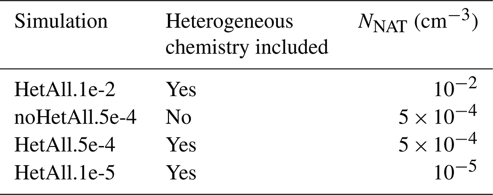
We performed sensitivity simulations varying the NAT number density within the observed range from 10−2 to 10−5 cm−3 in the current version 6 of WACCM. We also performed a simulation excluding stratospheric heterogeneous reactions, apart from the N2O5 + H2O reaction, to evaluate the impact of heterogeneous processes on the gas-phase species. The N2O5 + H2O reaction rate is nearly independent of temperature, also happens on the background aerosols, does not directly affect the halogen chemistry and is important for the partitioning of reactive nitrogen in the atmosphere; this is why we kept this reaction in that simulation. Without this reaction, the chemistry in the model would be completely unrealistic. All simulations are summarized in Table 1. They cover the satellite period starting from 1979 to the present.
Table 1Simulations in this study. In the “noHetAll” simulation, the heterogeneous reactions are removed apart from the N2O5 +H2O reaction.
2.2 The Michelson Interferometer for Passive Atmospheric Sounding (MIPAS)
The Michelson Interferometer for Passive Atmospheric Sounding (MIPAS) operated in limb geometry aboard the Environmental Satellite (Envisat) between July 2002 and April 2012 (Fischer et al., 2008). Envisat was placed in a sun-synchronous polar orbit at an altitude of around 800 km with more than 14 orbits per day. MIPAS measured a variety of trace gases including HNO3, ClONO2 and O3 using a Fourier transform spectrometer in the infrared spectral range between 4.15 and 14.6 µm at tangent altitudes from 7 to 72 km (Fischer et al., 2008). The spatial resolution was approximately 3 km in the vertical and 30 km in the horizontal. The spectral resolution was 0.05 cm−1 between 2002 and March 2004. Due to technical issues with the satellite and a corresponding gap in the measurements, MIPAS started measuring again in January 2005 with a reduced spectral resolution of 0.12 cm−1.
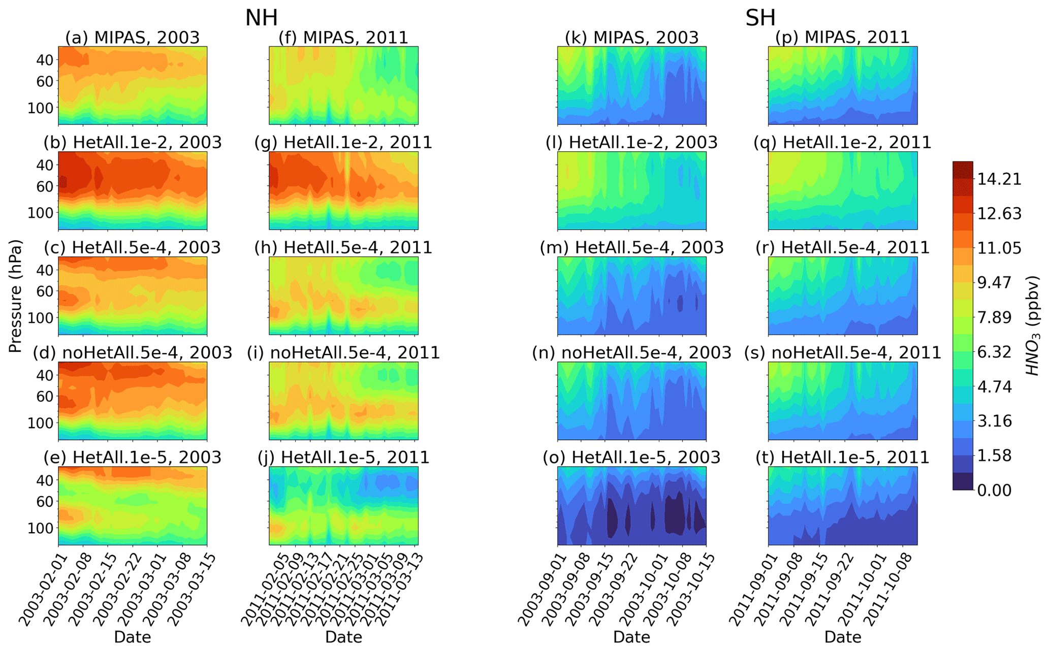
Figure 1Daily vortex-averaged HNO3 VMR profiles in the analyzed pressure range between 30 and 150 hPa during local spring for MIPAS (a, f, k, p) and the WACCM simulations (b–e, g–j, l–o, q–t) in the NH (a–j) and SH (k–t) and for the years 2003 and 2011 (the first and second columns in the hemispheres). The number of profiles used to average each day depends on the availability of MIPAS data and the size of the polar vortex.
For this study, we use the V8 Level-2 MIPAS retrievals from the IMK-IAA processor (Kiefer et al., 2021, 2023; von Clarmann et al., 2009) of HNO3, ClONO2 and O3 to compare their distributions with the WACCM simulations. The reported precision in the region between 30 and 150 hPa is 5 %–15 % (around 100 pptv) for HNO3 (Sheese et al., 2016, 2017), 10 % (around 150 ppbv) for O3 (Sheese et al., 2017; Kiefer et al., 2023) and 7 %–32 % (24–89 pptv) for ClONO2 (Sheese et al., 2016; Höpfner et al., 2007).
The method used to compare the MIPAS data with WACCM is based on the approach by Zambri et al. (2021). It takes advantage of WACCM's ability to provide output at the locations and times closest to the MIPAS profiles. In combination with interpolation of the MIPAS vertical levels to the WACCM altitudes, this enables a direct comparison of the two datasets. As a result, probability density functions (PDFs) can be evaluated in the spatiotemporal range of interest and compared to the observations.
As NAT formation and denitrification are strongly temperature dependent and most efficient at the lowest temperatures, we compute PDFs for profiles inside the polar vortex, determined by MERRA-2 using the Nash criterion (Nash et al., 1996). As the sedimentation of the NAT particles takes several weeks (Tabazadeh et al., 2001), the largest effects of denitrification can be expected to be most amplified after the local winter, which is why we restrict our analysis to the early local spring, i.e., 1 February to 15 March in the Northern Hemisphere and 1 September to 15 October in the Southern Hemisphere, and to the pressure range from 30 to 150 hPa. Sensitivity studies that involved changing these two ranges did not affect the main message of the results shown in the next section. In order to make the datasets comparable, we remove the profiles from both WACCM and MIPAS data where negative values occur in the measurements. This does not have a significant effect on the results. The number of profiles depends on the area of the polar vortex and differs from year to year. Generally, the number of profiles is larger in the SH due to the larger size of the SH polar vortex compared with the NH.
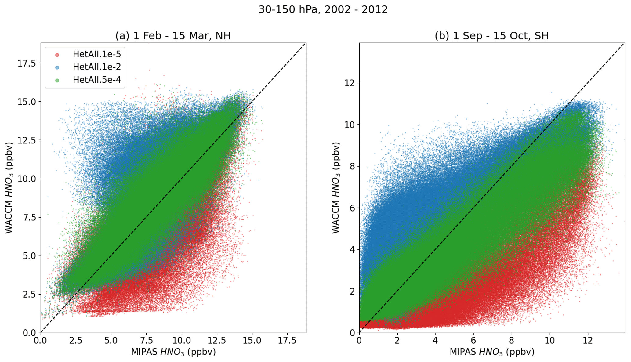
Figure 2Scatterplots of MIPAS and WACCM HNO3 in (a) the NH and (b) the SH for the HetAll simulation using the three NAT number densities described in the text. The dots include all measurement and model data between 30 and 150 hPa. The dashed line corresponds to the one-to-one line.
Zambri et al. (2021) used the Kolmogorov–Smirnov test to evaluate the difference in the PDFs between the model and observations, which uses the number of data points and the maximum difference between the cumulative density functions (CDFs) to check whether the distributions are distinguishable in a statistical sense related to a significance level α. Here, we use the maximum difference between the CDFs F of MIPAS and WACCM “max(d)” to directly evaluate the difference in the distributions (Zambri et al., 2021):
where x is the binned trace gas VMR. A more detailed discussion can be found in Zambri et al. (2021).
2.3 Ozonesondes
We also compare the WACCM simulations to balloon-borne in situ measurements of ozonesondes, made available by the World Ozone and Ultraviolet Data Centre. They use an electrochemical concentration cell to measure ozone profiles with a precision of 3 % to 5 % and an uncertainty of about ±10 % in the pressure range of interest here (Smit et al., 2007). We use ozonesondes of two stations: Eureka in the NH (80.04∘ N, 86.1∘ W) and Syowa in the SH (69.00∘ S, 39.58∘ E).
The method to compare the WACCM simulations with the ozonesonde measurements is similar to Wilka et al. (2021): the data are compared to the daily averaged WACCM ozone concentration at the grid point closest to the respective station for profiles within the polar vortex. Averages and spread of the differences between WACCM and the observations are evaluated.
In this section, we will analyze the influence of changing denitrification in WACCM on the trace gases HNO3, ClONO2 and O3 during early spring in both hemispheres. Generally, these species are expected to be influenced by a changed NAT number density because it leads to a redistribution of HNO3 (lower HNO3 at high altitudes and higher HNO3 at lower altitudes). During early spring, HNO3 is photolyzed and forms NO2 which combines with ClO to form ClONO2. ClO is responsible for part of the catalytic ozone depletion and deactivated by the reaction into ClONO2.
As a starting point, Fig. 1 shows vortex-mean profiles of the HNO3 VMR during the local spring months for both hemispheres and the years 2003 and 2011 for MIPAS and all WACCM simulations of this study. Analysis of the other years of the MIPAS period showed similar results, which is why we focus on the two example years 2003 and 2011 here. The signature of denitrification is indicated in the MIPAS measurements (first row of Fig. 1, panels a, f, k and p) by the HNO3 VMR decreasing over time at around 30 to 60 hPa, with corresponding increases due to renitrification at the end of the shown time series at lower levels, like in 2011 in the NH (Fig. 1f). In the simulation with the current operational NAT number density of 10−2 cm−3, HetAll.1e-2 in the second row of Fig. 1 (panels b, g, l and q), the NAT particles do not get large enough for the simulated HNO3 to compare well with the measured denitrification of the shown years. This means that larger HNO3 VMRs than observed remain at higher altitudes at the end of the time series, whereas the VMR is underestimated at lower altitudes. In contrast to this, with the smallest tested number density of 10−5 cm−3, HetAll.1e-5 in the last row of Fig. 1 (panels e, j, o and t), the HNO3 VMRs become too low, which indicates that the NAT particles become too large. By using a number density of cm−3 (HetAll.5e-4 in the third row of Fig. 1, panels d, i, n and s), the differences compared to MIPAS HNO3 are smallest and the altitude regions of denitrification and renitrification are comparable to the measurements.
In order to generalize this comparison, Fig. 2 shows correlation plots of the HetAll simulations using different NAT number densities compared with the MIPAS measurements for the whole pressure range (30–150 hPa) and all MIPAS years in the NH and SH. The HetAll.5e-4 simulation (green) has a relatively compact correlation with MIPAS in both hemispheres, whereas the other simulations show a larger scatter. The HetAll.1e-2 simulation shows HNO3 VMRs that are too large compared with the observations because of NAT particles that are too small. As already suggested by Fig. 1, the HNO3 VMRs in HetAll.1e-5 are too small compared with MIPAS as a result of overly large NAT particles which lead to sedimentation below the shown pressure range. As this figure includes the data of all MIPAS years and the whole pressure range, we will investigate the PDFs of this pressure range in the following, using the approach based on Zambri et al. (2021).
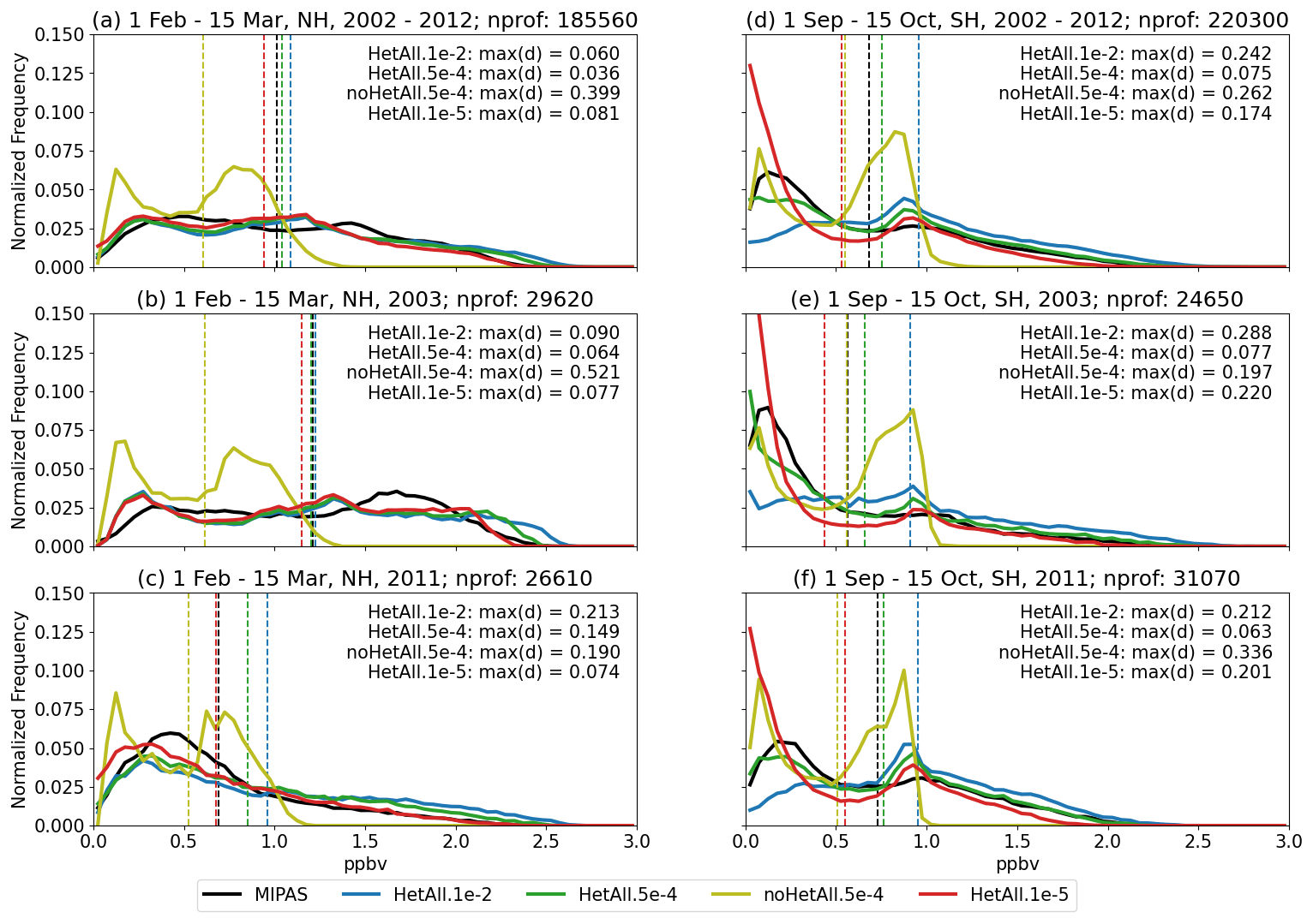
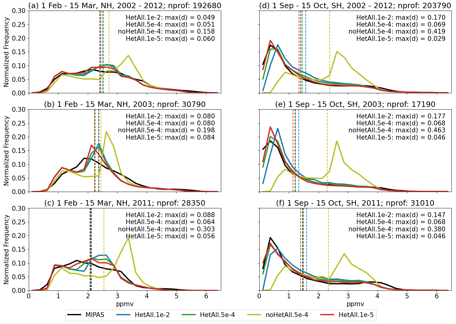
PDFs of HNO3 for the whole MIPAS period from 2002 to 2012 and for the years 2003 and 2011 are shown in Fig. 3 within the polar vortex in both hemispheres. All individual years can be found in the Supplement (Fig. S1). The blue line corresponds to the simulation with the largest NAT density, the red line shows the simulation with smallest NAT density, and the green and yellow lines show the simulations using cm−3, with the latter probing turning off all heterogeneous chemistry apart from N2O5 + H2O. The black line corresponds to the MIPAS HNO3 PDF.
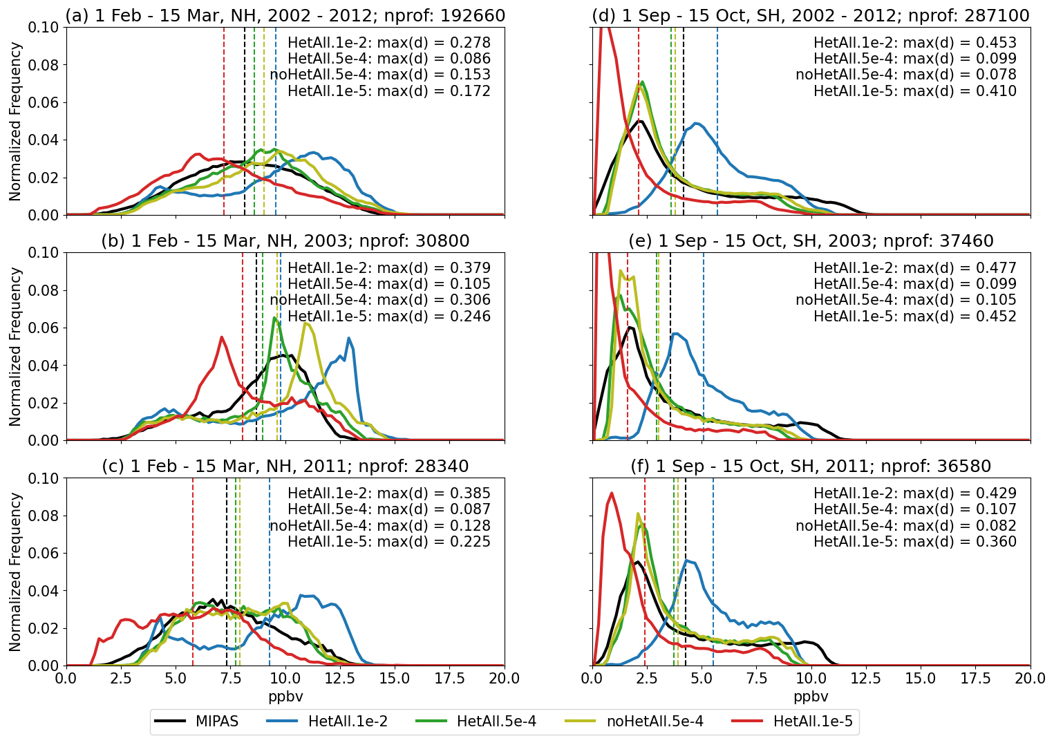
Figure 3HNO3 PDFs within the polar vortex for MIPAS and the sensitivity simulations of WACCM for the NH (a–c) and SH (d–f) spring months in (a, d) the MIPAS period from 2002 to 2012, (b, e) 2003 and (c, f) 2011. Vertical dashed lines show the average VMR of the respective simulations. The number of profiles used to derive the PDFs in each panel is denoted by “nprof”. The maximum differences between the CDFs of MIPAS and the respective WACCM simulation are denoted by “max(d)” in the panels.
Figure 3 demonstrates that the NAT density has a large impact on the PDFs in the model between 30 and 150 hPa. In HetAll.1e-2, larger HNO3 values are more frequent compared with the other simulations in all of the panels. In contrast to this, HetAll.1e-5 underestimates HNO3, as manifested by a higher frequency at smaller values. The simulation with peak values closest to the MIPAS observations in all panels of Fig. 3 is HetAll.5e-4, indicating that heterogeneous chemistry is relevant and that cm−3 leads to PDFs comparable to MIPAS for all years (see also Fig. S1). However, the NAT parameterization in WACCM is not able to capture the minimum and maximum values; this is especially notable in the SH where VMRs as high as 12.5 ppbv have been measured by MIPAS, whereas the largest values in HetAll.5e-4 are around 10 ppbv (e.g., in Fig. 3d).
The overall agreement is also shown by the mean values illustrated by the dashed vertical lines in the figure. Moreover, the mean HNO3 value for HetAll.5e-4 is closest to the MIPAS mean value in all of the panels. In addition, the maximum difference, max(d), of the HetAll.5e-4 simulations is smallest in the shown years compared with the other simulations.
In almost all years, heterogeneous chemistry leads to about 0.5 ppbv smaller HNO3 mixing ratios in the NH (see also Fig. S1). In the SH, this effect is not as large as in the NH. In total, the effect of halogen heterogeneous chemistry on HNO3 is small. The mean and shape of the distributions are similar for noHetAll.5e-4 and HetAll.5e-4.
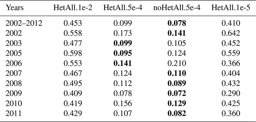
As the number of profiles differs from year to year depending on the development of the polar vortex, more weight in the distributions of the whole period from 2002 to 2012 (Fig. 3a and d) is given to years with a larger polar vortex. This is why the distributions of all individual years are shown in the Supplement (Figs. S1, S2, S3). As a summary, the max(d) values of the individual years are shown in Tables 2 and 3 for the NH and SH, respectively. The simulation with the minimum difference is highlighted in bold for each year. Apart from some exceptions in the NH, the minimum difference occurs for the simulations using cm−3. This is another indication that this value improves denitrification and the distribution of HNO3 in the polar vortex in both hemispheres.
Table 2Maximum differences between WACCM and MIPAS HNO3 CDFs (“max(d)” in the figures) for all years (1 February to 15 March in the NH). Bold font is used to highlight the minimum values in each row.
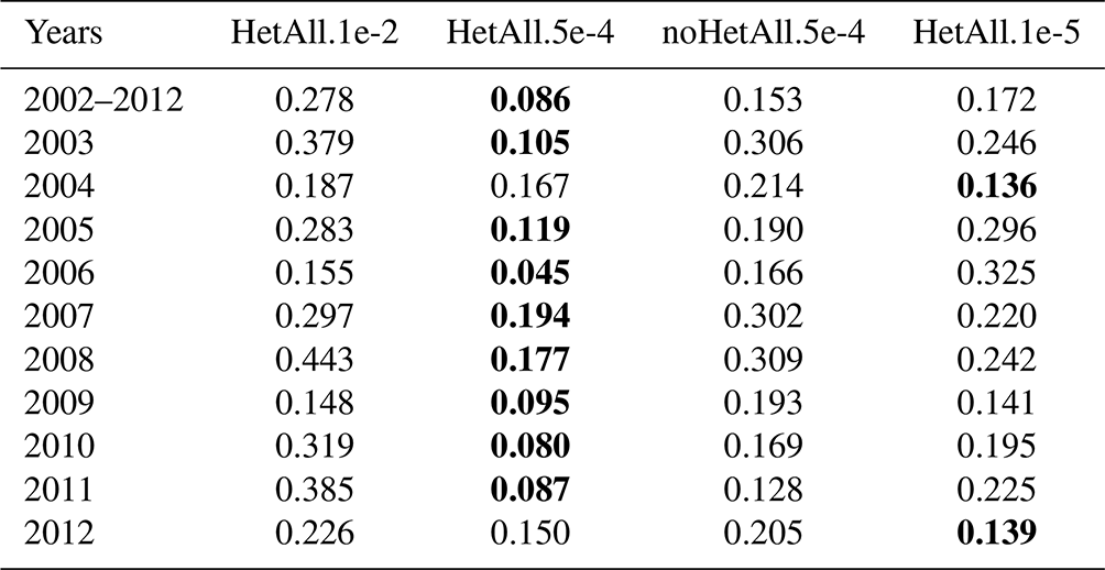
Table 3The same as Table 2 but for the SH spring (1 September to 15 October).
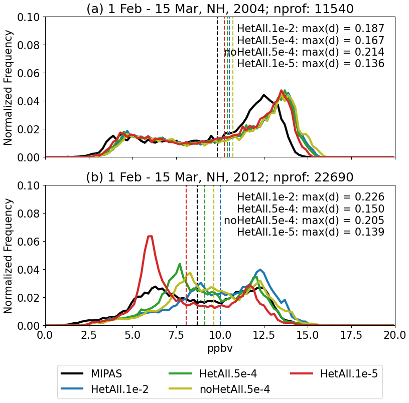
Exceptions are the years 2004 and 2012 in the NH, where the simulation with the smallest NAT density (HetAll.1e-5) shows the minimum differences compared with the MIPAS distribution (see Table 2). In 2004, relatively warm temperatures in the NH stratosphere lead to low denitrification (Manney et al., 2005). As shown in Fig. 4a, this is reflected by the WACCM HNO3 distributions which do not show large differences when changing the NAT density during that year. However, there seems to be a systematic difference between WACCM and MIPAS in this year, maybe due to a lower accuracy of the instrument or, for instance, a mismatch in the location of the polar vortex in the reanalysis data used for the model and the temperature history during that winter. The 2011/2012 Arctic winter was characterized by an early breakdown of the polar vortex at the end of December (Roy and Kuttippurath, 2022), but there is some evidence of large NAT particles during the cold period during December 2011 (Woiwode et al., 2019). This is why the HNO3 distributions change in WACCM and large NAT particles probably play a larger role in determining the distributions for that year (see Fig. 4b).
Moderate changes due to the different NAT densities can also be found in other species. Figure 5 shows the distributions of chlorine nitrate (ClONO2) for the same years and simulations as in Fig. 3. Both HetAll.1e-2 and HetAll.5e-4 have similar distributions and max(d) values. Depending on the year, minimum max(d) values occur in both simulations. HetAll.1e-5 seems to slightly underestimate the ClONO2 mixing ratios in both hemispheres, illustrated by higher frequencies of low mixing ratios.
As a result of increased denitrification, impacts on the maximum values in the ClONO2 distributions can be seen in both hemispheres. While the maximum ClONO2 mixing ratios in the NH are closer to the MIPAS distributions using cm−3, the HetAll.5e-4 simulation captures the maximum values in the SH distributions.
There is also a clear signature of heterogeneous chemistry in the ClONO2 distributions. The deactivation reaction forming ClONO2,
is usually faster than the deactivation reaction forming HCl,
as long as NO2 is available and the ozone VMRs are large enough (e.g., Kawa et al., 1992; Prather and Jaffe, 1990). At the edge regions of the polar vortex, some of the chlorine originally in HCl at the start of the winter shows up in ClONO2 at the end of the winter, known as the ClONO2 “collar” (e.g., Toon et al., 1989; Douglass et al., 1995; Solomon et al., 2016). Therefore, while the simulation without heterogeneous chemistry, noHetAll.5e-4, generally shows ClONO2 VMRs that are too low compared with MIPAS, it is notable that the maximum values are increased by about 1 ppbv and are then comparable to MIPAS in all simulations with heterogeneous chemistry.
Similar impacts can be seen in the distributions of ozone (O3), shown in Fig. 6. Ozone VMRs are about 1 ppmv too large in the SH for noHetAll.5e-4 compared with MIPAS. In the NH, the difference is smaller, but ozone is still overestimated in the simulation without heterogeneous chemistry.
Wilka et al. (2021) showed that the agreement of WACCM model calculations of Arctic spring ozone losses in 2020 with ozonesonde data was heavily dependent on the denitrification parameterization used in the model, providing an important check. Figure 7 displays comparisons between WACCM and ozonesonde data at Syowa and Eureka for their respective spring seasons for all years between 2002 and 2012. A figure showing the comparison to Syowa without noHetAll.5e-4 can be found in the Supplement (Fig. S4). Similar comparisons are provided for the South Pole in Fig. S5. Because local Antarctic ozone abundances can drop to values lower than 1 ppmv between about 15 and 20 km in years with large ozone losses (see, e.g., Fig. 7a), care must be taken in interpreting percentage differences; we also provide absolute differences for that reason. The Syowa sondes agree considerably better with the model when the NAT number density of cm−3 or less is used, compared with larger values of this parameter. At Eureka, results are far less sensitive due to smaller ozone losses, except in very cold years (like the year 2020, as shown in Wilka et al., 2021).
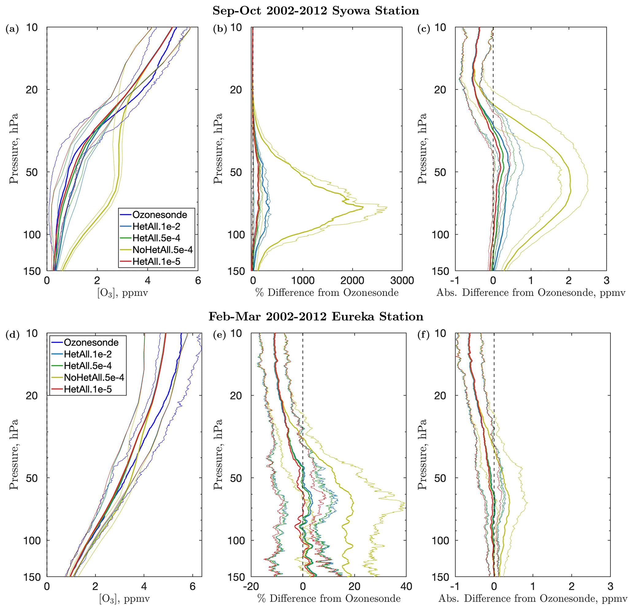
Figure 7Mean and interquartile (0.25 and 0.75) range of (a, d) the volume mixing ratio as well as (b, e) relative differences and (c, f) absolute differences between the respective WACCM simulations and two ozonesonde stations for profiles within the polar vortex using the same definition as in the previous analysis. Panels (a)–(c) show Syowa Station in the Antarctic, and panels (d)–(f) show Eureka Station in the Arctic. For WACCM, the grid point closest to the station is chosen. The average and distributions are taken for all profiles within the MIPAS period and the same months as for the satellite comparison. The first column (a, d) shows the O3 VMR, the second column (b, e) shows the relative difference between WACCM and the ozonesonde measurements, and the third column (c, f) shows the absolute difference between WACCM and the ozonesonde measurements.
In summary, the results in this section showed that the diagnostic parameterization of NAT particles in WACCM is able to reflect the main features in the three key gas-phase species, HNO3, ClONO2 and ozone. When using a reduced NAT particle number density of cm−3 compared with the standard WACCM setup, the difference in the CDFs is minimized for almost all spring months of the MIPAS period from 2002 to 2012, and the bias between 30 and 150 hPa in comparison to the ozonesondes is reduced. This indicates that cm−3 improves the distribution of these species in the polar regions and that it should be used in future WACCM simulations.
In this study, we investigated the impact of the NAT number density (NNAT) on the distributions of key gaseous species in the WACCM model. We compared PDFs within the polar vortex with the MIPAS satellite instrument which operated between 2002 and 2012. As a measure of the difference between the distributions of WACCM and MIPAS, we used the maximum difference, max(d), between the CDFs. To identify the impact of NAT on the distributions of the species, we performed sensitivity simulations varying NNAT between 10−2 and 10−5 cm−3. In the method applied here to compare the satellite measurements with the model, negative values in the satellite retrievals are cut off, which is why the method cannot be used for noisy data (such as N2O5 and ClO in MIPAS) and we restricted the analysis to the gaseous species HNO3, ClONO2 and O3.
The diagnostic parameterization of NAT in the WACCM model was shown to be able to reproduce the general shape of the MIPAS distributions for almost all years of the MIPAS period in the polar vortices of both hemispheres. However, there was a general overestimation of gaseous HNO3 when using the standard NNAT of 10−2 cm−3. Reducing this number concentration to cm−3 was shown to also reduce the differences in the HNO3 distributions between MIPAS and WACCM for almost all spring seasons in both hemispheres during the MIPAS period. Changes in the distributions of ClONO2 and O3 due to the new value of NNAT were either negligible or the differences were reduced. Mean differences between the ozonesonde profiles and the WACCM simulations at the grid point closest to the Syowa and Eureka sonde stations were also shown to be decreased when reducing NNAT. Therefore, this study suggests the use of cm−3 for future simulations. This new value is within the range of measured NAT number densities.
A simplified parameterization as applied in WACCM cannot capture all features of the distributions of all years. This was demonstrated by the years 2004 and 2012 where differences between the MIPAS and WACCM distributions were increased. Further, there are many uncertainties in the detailed chemistry from one year to another that may also be important for denitrification and ozone loss, including, for example, volcanic particle inputs, gravity and planetary wave amplitudes, and changes in circulation, to name only a few. It can also be seen that the smallest number density of 10−5 cm−3 is comparable to measurements during the exceptionally cold northern winter of 2019/2020 (Wilka et al., 2021). In addition, although overall differences in the PDFs are reduced with cm−3, the Kolmogorov–Smirnov test, used by studies such as Zambri et al. (2021) with a similar approach to that used in this study, will fail if it does not employ a significance level α that is set to a very small value (O(10−70)). Therefore, although the differences are decreased, the distributions of MIPAS and WACCM are still different in a statistical sense, probably due to the simplifications in the NAT parameterization of WACCM.
Future studies could apply this methodology to other long-term satellite measurements to evaluate the usage of this new NAT number density for further years, although their precision has to be low enough to allow for comparisons with individual profiles. Nevertheless, as a follow-up of the publication by Wilka et al. (2021), we recommend using cm−3 for future simulations with WACCM, indicating that NAT rocks play an important role, especially in the NH where we saw the largest impact on changing the NAT number density.
Instructions on how to access MIPAS data can be found at https://www.imk-asf.kit.edu/english/308.php (MIPAS Science Team, 2023). Instructions on how to download CESM version 2 can be found in Danabasoglu et al. (2020). Ozonesonde station data are publicly available through the World Ozone and Ultraviolet Data Center (WOUDC; https://doi.org/10.14287/10000001; WMO/GAW Ozone Monitoring Community, 2022). The scripts and data needed to create the figures of this paper can be found at https://g-27eb33.7a577b.6fbd.data.globus.org/ACP_Weimer_2022/ACP_Weimer_2022.tar.gz (Weimer et al., 2023).
The supplement related to this article is available online at: https://doi.org/10.5194/acp-23-6849-2023-supplement.
MW added the comparison with MIPAS and wrote the first draft of the manuscript. DEK performed the simulations with WACCM used for the comparisons. CW added the comparison to ozonesondes. All authors contributed to the manuscript preparation.
The contact author has declared that none of the authors has any competing interests.
Publisher's note: Copernicus Publications remains neutral with regard to jurisdictional claims in published maps and institutional affiliations.
Michael Weimer and Douglas E. Kinnison were funded in part by NASA (grant no. 80NSSC19K0952). Susan Solomon was funded in part by the US National Science Foundation (NSF; grant no. 1906719). We would like to thank Brian Zambri for initiating this work and helping with the comparison to MIPAS. This material is based upon work supported by the National Center for Atmospheric Research (NCAR), which is a major facility sponsored by the NSF under Cooperative Agreement No. 1852977. The CESM project is supported primarily by the NSF. We would like to acknowledge support from the Svante cluster at Massachusetts Institute of Technology used for the comparison of the model and the data (see https://svante.mit.edu/intro.html, last access: 18 November 2022, for more information). We would like to acknowledge high-performance computing support from Cheyenne and Casper provided by NCAR's Computational and Information Systems Laboratory (2019), sponsored by the NSF.
This research has been supported by the National Aeronautics and Space Administration (grant no. 80NSSC19K0952) and the National Science Foundation (grant no. AGS-1906719).
This paper was edited by Farahnaz Khosrawi and reviewed by Ingo Wohltmann and one anonymous referee.
Adriani, A., Massoli, P., Di Donfrancesco, G., Cairo, F., Moriconi, M. L., and Snels, M.: Climatology of polar stratospheric clouds based on lidar observations from 1993 to 2001 over McMurdo Station, Antarctica, J. Geophys. Res.-Atmos., 109, 1–17, https://doi.org/10.1029/2004JD004800, 2004. a
Carslaw, K. S., Luo, B. P., Clegg, S. L., Peter, T., Brimblecombe, P., and Crutzen, P. J.: Stratospheric aerosol growth and HNO3 gas phase depletion from coupled HNO3 and water uptake by liquid particles, Geophys. Res. Lett., 21, 2479–2482, https://doi.org/10.1029/94GL02799, 1994. a
Carslaw, K. S., Wirth, M., Tsias, A., Luo, B. P., Dörnbrack, A., Leutbecher, M., Volkert, H., Renger, W., Bacmeister, J. T., and Peter, T.: Particle microphysics and chemistry in remotely observed mountain polar stratospheric clouds, J. Geophys. Res.-Atmos., 103, 5785–5796, https://doi.org/10.1029/97JD03626, 1998. a
Carslaw, K. S., Kettleborough, J. A., Northway, M. J., Davies, S., Gao, R.-S., Fahey, D. W., Baumgardner, D. G., Chipperfield, M. P., and Kleinböhl, A.: A vortex-scale simulation of the growth and sedimentation of large nitric acid hydrate particles, J. Geophys. Res.-Atmos., 107, SOL 43-1–SOL 43-16, https://doi.org/10.1029/2001JD000467, 2002. a
Computational and Information Systems Laboratory: Cheyenne: HPE/SGI ICE XA System (University Community Computing), Tech. rep., National Center for Atmospheric Research, Boulder, CO, https://doi.org/10.5065/D6RX99HX, 2019. a
Considine, D. B., Douglass, A. R., Connell, P. S., Kinnison, D. E., and Rotman, D. A.: A polar stratospheric cloud parameterization for the global modeling initiative three-dimensional model and its response to stratospheric aircraft, J. Geophys. Res.-Atmos., 105, 3955–3973, https://doi.org/10.1029/1999JD900932, 2000. a, b, c, d
Danabasoglu, G., Lamarque, J. F., Bacmeister, J., Bailey, D. A., DuVivier, A. K., Edwards, J., Emmons, L. K., Fasullo, J., Garcia, R., Gettelman, A., Hannay, C., Holland, M. M., Large, W. G., Lauritzen, P. H., Lawrence, D. M., Lenaerts, J. T., Lindsay, K., Lipscomb, W. H., Mills, M. J., Neale, R., Oleson, K. W., Otto-Bliesner, B., Phillips, A. S., Sacks, W., Tilmes, S., van Kampenhout, L., Vertenstein, M., Bertini, A., Dennis, J., Deser, C., Fischer, C., Fox-Kemper, B., Kay, J. E., Kinnison, D., Kushner, P. J., Larson, V. E., Long, M. C., Mickelson, S., Moore, J. K., Nienhouse, E., Polvani, L., Rasch, P. J., and Strand, W. G.: The Community Earth System Model Version 2 (CESM2), J. Adv. Model. Earth Syst., 12, e2019MS001916, https://doi.org/10.1029/2019MS001916, 2020. a, b
Douglass, A. R., Schoeberl, M. R., Stolarski, R. S., Waters, J. W., Russell III, J. M., Roche, A. E., and Massie, S. T.: Interhemispheric differences in springtime production of HCl and ClONO2 in the polar vortices, J. Geophys. Res.-Atmos., 100, 13967–13978, https://doi.org/10.1029/95JD00698, 1995. a
Drdla, K. and Müller, R.: Temperature thresholds for chlorine activation and ozone loss in the polar stratosphere, Ann. Geophys., 30, 1055–1073, https://doi.org/10.5194/angeo-30-1055-2012, 2012. a
Fahey, D. W.: The Detection of Large HNO3-Containing Particles in the Winter Arctic Stratosphere, Science, 291, 1026–1031, https://doi.org/10.1126/science.1057265, 2001. a, b, c, d
Fahey, D. W., Kelly, K. K., Ferry, G. V., Poole, L. R., Wilson, J. C., Murphy, D. M., Loewenstein, M., and Chan, K. R.: In situ measurements of total reactive nitrogen, total water, and aerosol in a polar stratospheric cloud in the Antarctic, J. Geophys. Res., 94, 11299, https://doi.org/10.1029/JD094iD09p11299, 1989. a
Fischer, H., Birk, M., Blom, C., Carli, B., Carlotti, M., von Clarmann, T., Delbouille, L., Dudhia, A., Ehhalt, D., Endemann, M., Flaud, J. M., Gessner, R., Kleinert, A., Koopman, R., Langen, J., López-Puertas, M., Mosner, P., Nett, H., Oelhaf, H., Perron, G., Remedios, J., Ridolfi, M., Stiller, G., and Zander, R.: MIPAS: an instrument for atmospheric and climate research, Atmos. Chem. Phys., 8, 2151–2188, https://doi.org/10.5194/acp-8-2151-2008, 2008. a, b
Fueglistaler, S., Luo, B. P., Voigt, C., Carslaw, K. S., and Peter, Th.: NAT-rock formation by mother clouds: a microphysical model study, Atmos. Chem. Phys., 2, 93–98, https://doi.org/10.5194/acp-2-93-2002, 2002. a
Gelaro, R., McCarty, W., Suárez, M. J., Todling, R., Molod, A., Takacs, L., Randles, C. A., Darmenov, A., Bosilovich, M. G., Reichle, R., Wargan, K., Coy, L., Cullather, R., Draper, C., Akella, S., Buchard, V., Conaty, A., da Silva, A. M., Gu, W., Kim, G.-K., Koster, R., Lucchesi, R., Merkova, D., Nielsen, J. E., Partyka, G., Pawson, S., Putman, W., Rienecker, M., Schubert, S. D., Sienkiewicz, M., and Zhao, B.: The Modern-Era Retrospective Analysis for Research and Applications, Version 2 (MERRA-2), J. Climate, 30, 5419–5454, https://doi.org/10.1175/JCLI-D-16-0758.1, 2017. a
Gettelman, A., Mills, M. J., Kinnison, D. E., Garcia, R. R., Smith, A. K., Marsh, D. R., Tilmes, S., Vitt, F., Bardeen, C. G., McInerny, J., Liu, H. L., Solomon, S. C., Polvani, L. M., Emmons, L. K., Lamarque, J. F., Richter, J. H., Glanville, A. S., Bacmeister, J. T., Phillips, A. S., Neale, R. B., Simpson, I. R., DuVivier, A. K., Hodzic, A., and Randel, W. J.: The Whole Atmosphere Community Climate Model Version 6 (WACCM6), J. Geophys. Res.-Atmos., 124, 12380–12403, https://doi.org/10.1029/2019JD030943, 2019. a
Grooß, J.-U., Günther, G., Müller, R., Konopka, P., Bausch, S., Schlager, H., Voigt, C., Volk, C. M., and Toon, G. C.: Simulation of denitrification and ozone loss for the Arctic winter 2002/2003, Atmos. Chem. Phys., 5, 1437–1448, https://doi.org/10.5194/acp-5-1437-2005, 2005. a
Hanson, D. and Mauersberger, K.: Laboratory studies of the nitric acid trihydrate: Implications for the south polar stratosphere, Geophys. Res. Lett., 15, 855–858, https://doi.org/10.1029/GL015i008p00855, 1988. a
Höpfner, M., Larsen, N., Spang, R., Luo, B. P., Ma, J., Svendsen, S. H., Eckermann, S. D., Knudsen, B., Massoli, P., Cairo, F., Stiller, G., von Clarmann, T., and Fischer, H.: MIPAS detects Antarctic stratospheric belt of NAT PSCs caused by mountain waves, Atmos. Chem. Phys., 6, 1221–1230, https://doi.org/10.5194/acp-6-1221-2006, 2006. a
Höpfner, M., Von Clarmann, T., Fischer, H., Funke, B., Glatthor, N., Grabowski, U., Kellmann, S., Kiefer, M., Linden, A., Milz, M., Steck, T., Stiller, G. P., Bernath, P., Blom, C. E., Blumenstock, T., Boone, C., Chance, K., Coffey, M. T., Friedl-Vallon, F., Griffith, D., Hannigan, J. W., Hase, F., Jones, N., Jucks, K. W., Keim, C., Kleinert, A., Kouker, W., Liu, G. Y., Mahieu, E., Mellqvist, J., Mikuteit, S., Notholt, J., Oelhaf, H., Piesch, C., Reddmann, T., Ruhnke, R., Schneider, M., Strandberg, A., Toon, G., Walker, K. A., Warneke, T., Wetzel, G., Wood, S., and Zander, R.: Validation of MIPAS ClONO2 measurements, Atmos. Chem. Phys., 7, 257–281, https://doi.org/10.5194/acp-7-257-2007, 2007. a
Höpfner, M., Deshler, T., Pitts, M., Poole, L., Spang, R., Stiller, G., and von Clarmann, T.: The MIPAS/Envisat climatology (2002–2012) of polar stratospheric cloud volume density profiles, Atmos. Meas. Tech., 11, 5901–5923, https://doi.org/10.5194/amt-11-5901-2018, 2018. a
Kawa, S. R., Fahey, D. W., Heidt, L. E., Pollock, W. H., Solomon, S., Anderson, D. E., Loewenstein, M., Proffitt, M. H., Margitan, J. J., and Chan, K. R.: Photochemical partitioning of the reactive nitrogen and chlorine reservoirs in the high-latitude stratosphere, J. Geophys. Res.-Atmos., 97, 7905–7923, https://doi.org/10.1029/91JD02399, 1992. a
Kelly, K. K., Tuck, A. F., Murphy, D. M., Proffitt, M. H., Fahey, D. W., Jones, R. L., McKenna, D. S., Loewenstein, M., Podolske, J. R., Strahan, S. E., Ferry, G. V., Chan, K. R., Vedder, J. F., Gregory, G. L., Hypes, W. D., McCormick, M. P., Browell, E. V., and Heidt, L. E.: Dehydration in the lower Antarctic stratosphere during late winter and early spring, 1987, J. Geophys. Res., 94, 11317, https://doi.org/10.1029/JD094iD09p11317, 1989. a
Kiefer, M., von Clarmann, T., Funke, B., García-Comas, M., Glatthor, N., Grabowski, U., Kellmann, S., Kleinert, A., Laeng, A., Linden, A., López-Puertas, M., Marsh, D. R., and Stiller, G. P.: IMK/IAA MIPAS temperature retrieval version 8: nominal measurements, Atmos. Meas. Tech., 14, 4111–4138, https://doi.org/10.5194/amt-14-4111-2021, 2021. a
Kiefer, M., von Clarmann, T., Funke, B., García-Comas, M., Glatthor, N., Grabowski, U., Höpfner, M., Kellmann, S., Laeng, A., Linden, A., López-Puertas, M., and Stiller, G. P.: Version 8 IMK–IAA MIPAS ozone profiles: nominal observation mode, Atmos. Meas. Tech., 16, 1443–1460, https://doi.org/10.5194/amt-16-1443-2023, 2023. a, b
Kinnison, D. E., Brasseur, G. P., Walters, S., Garcia, R. R., Marsh, D. R., Sassi, F., Harvey, V. L., Randall, C. E., Emmons, L., Lamarque, J. F., Hess, P., Orlando, J. J., Tie, X. X., Randel, W., Pan, L. L., Gettelman, A., Granier, C., Diehl, T., Niemeier, U., and Simmons, A. J.: Sensitivity of chemical tracers to meteorological parameters in the MOZART-3 chemical transport model, J. Geophys. Res.-Atmos., 112, 20302, https://doi.org/10.1029/2006JD007879, 2007. a
Kirner, O., Ruhnke, R., Buchholz-Dietsch, J., Jöckel, P., Brühl, C., and Steil, B.: Simulation of polar stratospheric clouds in the chemistry-climate-model EMAC via the submodel PSC, Geosci. Model Dev., 4, 169–182, https://doi.org/10.5194/gmd-4-169-2011, 2011. a, b
Manney, G. L., Krüger, K., Sabutis, J. L., Sena, S. A., and Pawson, S.: The remarkable 2003–2004 winter and other recent warm winters in the Arctic stratosphere since the late 1990s, J. Geophys. Res.-Atmos., 110, 1–14, https://doi.org/10.1029/2004JD005367, 2005. a
MIPAS Science Team: Access to IMK/IAA generated MIPAS/Envisat data, https://www.imk-asf.kit.edu/english/308.php (last access 16 June 2023), 2023. a
Molleker, S., Borrmann, S., Schlager, H., Luo, B., Frey, W., Klingebiel, M., Weigel, R., Ebert, M., Mitev, V., Matthey, R., Woiwode, W., Oelhaf, H., Dörnbrack, A., Stratmann, G., Grooß, J.-U., Günther, G., Vogel, B., Müller, R., Krämer, M., Meyer, J., and Cairo, F.: Microphysical properties of synoptic-scale polar stratospheric clouds: in situ measurements of unexpectedly large HNO3-containing particles in the Arctic vortex, Atmos. Chem. Phys., 14, 10785–10801, https://doi.org/10.5194/acp-14-10785-2014, 2014. a
Nash, E. R., Newman, P. A., Rosenfield, J. E., and Schoeberl, M. R.: An objective determination of the polar vortex using Ertel's potential vorticity, J. Geophys. Res.-Atmos., 101, 9471–9478, https://doi.org/10.1029/96JD00066, 1996. a
Peter, T.: Microphysics and heterogeneous chemistry of polar stratospheric clouds, Annu. Rev. Phys. Chem., 48, 785–822, https://doi.org/10.1146/annurev.physchem.48.1.785, 1997. a
Pitts, M. C., Poole, L. R., and Thomason, L. W.: CALIPSO polar stratospheric cloud observations: second-generation detection algorithm and composition discrimination, Atmos. Chem. Phys., 9, 7577–7589, https://doi.org/10.5194/acp-9-7577-2009, 2009. a, b
Pitts, M. C., Poole, L. R., Dörnbrack, A., and Thomason, L. W.: The 2009–2010 Arctic polar stratospheric cloud season: a CALIPSO perspective, Atmos. Chem. Phys., 11, 2161–2177, https://doi.org/10.5194/acp-11-2161-2011, 2011. a, b
Pitts, M. C., Poole, L. R., and Gonzalez, R.: Polar stratospheric cloud climatology based on CALIPSO spaceborne lidar measurements from 2006 to 2017, Atmos. Chem. Phys., 18, 10881–10913, https://doi.org/10.5194/acp-18-10881-2018, 2018. a
Prather, M. and Jaffe, A. H.: Global impact of the Antarctic ozone hole: Chemical propagation, J. Geophys. Res.-Atmos., 95, 3473–3492, https://doi.org/10.1029/JD095iD04p03473, 1990. a
Roy, R. and Kuttippurath, J.: The dynamical evolution of Sudden Stratospheric Warmings of the Arctic winters in the past decade 2011–2021, SN Appl. Sci., 4, 1–12, https://doi.org/10.1007/S42452-022-04983-4, 2022. a
Santee, M. L., Lambert, A., Read, W. G., Livesey, N. J., Cofield, R. E., Cuddy, D. T., Daffer, W. H., Drouin, B. J., Froidevaux, L., Fuller, R. A., Jarnot, R. F., Knosp, B. W., Manney, G. L., Perun, V. S., Snyder, W. V., Stek, P. C., Thurstans, R. P., Wagner, P. A., Waters, J. W., Muscari, G., de Zafra, R. L., Dibb, J. E., Fahey, D. W., Popp, P. J., Marcy, T. P., Jucks, K. W., Toon, G. C., Stachnik, R. A., Bernath, P. F., Boone, C. D., Walker, K. A., Urban, J., and Murtagh, D.: Validation of the Aura Microwave Limb Sounder HNO3 measurements, J. Geophys. Res.-Atmos., 112, 24–40, https://doi.org/10.1029/2007JD008721, 2007. a
Schoeberl, M. R., Lait, L. R., Newman, P. A., and Rosenfield, J. E.: The structure of the polar vortex, J. Geophys. Res.-Atmos., 97, 7859–7882, https://doi.org/10.1029/91JD02168, 1992. a
Sheese, P. E., Walker, K. A., Boone, C. D., McLinden, C. A., Bernath, P. F., Bourassa, A. E., Burrows, J. P., Degenstein, D. A., Funke, B., Fussen, D., Manney, G. L., Thomas McElroy, C., Murtagh, D., Randall, C. E., Raspollini, P., Rozanov, A., Russell, J. M., Suzuki, M., Shiotani, M., Urban, J., Von Clarmann, T., and Zawodny, J. M.: Validation of ACE-FTS version 3.5 NOy species profiles using correlative satellite measurements, Atmos. Meas. Tech., 9, 5781–5810, https://doi.org/10.5194/amt-9-5781-2016, 2016. a, b
Sheese, P. E., Walker, K. A., Boone, C. D., Bernath, P. F., Froidevaux, L., Funke, B., Raspollini, P., and von Clarmann, T.: ACE-FTS ozone, water vapour, nitrous oxide, nitric acid, and carbon monoxide profile comparisons with MIPAS and MLS, J. Quant. Spectrosc. Ra., 186, 63–80, https://doi.org/10.1016/J.JQSRT.2016.06.026, 2017. a, b
Smit, H. G. J., Straeter, W., Johnson, B. J., Oltmans, S. J., Davies, J., Tarasick, D. W., Hoegger, B., Stubi, R., Schmidlin, F. J., Northam, T., Thompson, A. M., Witte, J. C., Boyd, I., and Posny, F.: Assessment of the performance of ECC-ozonesondes under quasi-flight conditions in the environmental simulation chamber: Insights from the Juelich Ozone Sonde Intercomparison Experiment (JOSIE), J. Geophys. Res.-Atmos., 112, D19306, https://doi.org/10.1029/2006JD007308, 2007. a
Solomon, S.: Stratospheric ozone depletion: A review of concepts and history, Rev. Geophys., 37, 275–316, https://doi.org/10.1029/1999RG900008, 1999. a
Solomon, S., Garcia, R. R., Rowland, F. S., and Wuebbles, D. J.: On the depletion of Antarctic ozone, Nature, 321, 755–758, https://doi.org/10.1038/321755a0, 1986. a
Solomon, S., Kinnison, D., Bandoro, J., and Garcia, R.: Simulation of polar ozone depletion: An update, J. Geophys. Res.-Atmos., 120, 7958–7974, https://doi.org/10.1002/2015JD023365, 2015. a
Solomon, S., Kinnison, D., Garcia, R. R., Bandoro, J., Mills, M., Wilka, C., Neely, R. R., Schmidt, A., Barnes, J. E., Vernier, J. P., and Höpfner, M.: Monsoon circulations and tropical heterogeneous chlorine chemistry in the stratosphere, Geophys. Res. Lett., 43, 12624–12633, https://doi.org/10.1002/2016GL071778, 2016. a
Spang, R., Hoffmann, L., Müller, R., Grooß, J.-U., Tritscher, I., Höpfner, M., Pitts, M., Orr, A., and Riese, M.: A climatology of polar stratospheric cloud composition between 2002 and 2012 based on MIPAS/Envisat observations, Atmos. Chem. Phys., 18, 5089–5113, https://doi.org/10.5194/acp-18-5089-2018, 2018. a
Tabazadeh, A., Jensen, E. J., Toon, O. B., Drdla, K., and Schoeberl, M. R.: Role of the Stratospheric Polar Freezing Belt in Denitrification, Science, 291, 2591–2594, https://doi.org/10.1126/science.1057228, 2001. a
Toon, G. C., Farmer, C. B., Lowes, L. L., Schaper, P. W., Blavier, J.-F., and Norton, R. H.: Infrared aircraft measurements of stratospheric composition over Antarctica during September 1987, J. Geophys. Res.-Atmos., 94, 16571–16596, https://doi.org/10.1029/JD094iD14p16571, 1989. a
Tritscher, I., Pitts, M. C., Poole, L. R., Alexander, S. P., Cairo, F., Chipperfield, M. P., Grooß, J., Höpfner, M., Lambert, A., Luo, B., Molleker, S., Orr, A., Salawitch, R., Snels, M., Spang, R., Woiwode, W., and Peter, T.: Polar Stratospheric Clouds: Satellite Observations, Processes, and Role in Ozone Depletion, Rev. Geophys., 59, e2020RG000702, https://doi.org/10.1029/2020RG000702, 2021. a
Voigt, C., Schreiner, J., Kohlmann, A., Zink, P., Mauersberger, K., Larsen, N., Deshler, T., Kroger, C., Rosen, J., Adriani, A., Cairo, F., Di Donfrancesco, G., Viterbin, M., Ovarlez, J., Ovarlez, H., David, C., and Dornbrack, A.: Nitric Acid Trihydrate (NAT) in Polar Stratospheric Clouds, Science, 290, 1756–1758, https://doi.org/10.1126/SCIENCE.290.5497.1756, 2000. a
Voigt, C., Schlager, H., Luo, B. P., Dörnbrack, A., Roiger, A., Stock, P., Curtius, J., Vössing, H., Borrmann, S., Davies, S., Konopka, P., Schiller, C., Shur, G., and Peter, T.: Nitric Acid Trihydrate (NAT) formation at low NAT supersaturation in Polar Stratospheric Clouds (PSCs), Atmos. Chem. Phys., 5, 1371–1380, https://doi.org/10.5194/acp-5-1371-2005, 2005. a
von Clarmann, T., Höpfner, M., Kellmann, S., Linden, A., Chauhan, S., Funke, B., Grabowski, U., Glatthor, N., Kiefer, M., Schieferdecker, T., Stiller, G. P., and Versick, S.: Retrieval of temperature, H2O, O3, HNO3, CH4, N2O, ClONO2 and ClO from MIPAS reduced resolution nominal mode limb emission measurements, Atmos. Meas. Tech., 2, 159–175, https://doi.org/10.5194/amt-2-159-2009, 2009. a
Waibel, A. E., Peter, T., Carslaw, K. S., Oelhaf, H., Wetzel, G., Crutzen, P. J., Pöschl, U., Tsias, A., Reimer, E., and Fischer, H.: Arctic Ozone Loss Due to Denitrification, Science, 283, 2064–2069, https://doi.org/10.1126/science.283.5410.2064, 1999. a
Wegner, T., Kinnison, D. E., Garcia, R. R., and Solomon, S.: Simulation of polar stratospheric clouds in the specified dynamics version of the whole atmosphere community climate model, J. Geophys. Res.-Atmos., 118, 4991–5002, https://doi.org/10.1002/jgrd.50415, 2013. a, b, c, d, e
Weimer, M., Buchmüller, J., Hoffmann, L., Kirner, O., Luo, B., Ruhnke, R., Steiner, M., Tritscher, I., and Braesicke, P.: Mountain-wave-induced polar stratospheric clouds and their representation in the global chemistry model ICON-ART, Atmos. Chem. Phys., 21, 9515–9543, https://doi.org/10.5194/acp-21-9515-2021, 2021. a, b
Weimer, M., Kinnison, D. E., Wilka, C., and Solomon, S.: ACP_Weimer_2022, https://g-27eb33.7a577b.6fbd.data.globus.org/ACP_Weimer_2022/ACP_Weimer_2022.tar.gz (last access: 16 June 2023), 2023. a
Wespes, C., Ronsmans, G., Clarisse, L., Solomon, S., Hurtmans, D., Clerbaux, C., and Coheur, P.-F.: Polar stratospheric nitric acid depletion surveyed from a decadal dataset of IASI total columns, Atmos. Chem. Phys., 22, 10993–11007, https://doi.org/10.5194/acp-22-10993-2022, 2022. a
Wilka, C., Solomon, S., Kinnison, D., and Tarasick, D.: An Arctic ozone hole in 2020 if not for the Montreal Protocol, Atmos. Chem. Phys., 21, 15771–15781, https://doi.org/10.5194/acp-21-15771-2021, 2021. a, b, c, d, e, f
WMO/GAW Ozone Monitoring Community: World Meteorological Organization-Global Atmosphere Watch Program (WMO-GAW): Ozone, WOUDC – World Ozone and Ultraviolet Radiation Data Centre [data set], https://doi.org/10.14287/10000001, 2022. a
Wohltmann, I., Lehmann, R., and Rex, M.: The Lagrangian chemistry and transport model ATLAS: simulation and validation of stratospheric chemistry and ozone loss in the winter 1999/2000, Geosci. Model Dev., 3, 585–601, https://doi.org/10.5194/gmd-3-585-2010, 2010. a
Woiwode, W., Grooß, J.-U., Oelhaf, H., Molleker, S., Borrmann, S., Ebersoldt, A., Frey, W., Gulde, T., Khaykin, S., Maucher, G., Piesch, C., and Orphal, J.: Denitrification by large NAT particles: the impact of reduced settling velocities and hints on particle characteristics, Atmos. Chem. Phys., 14, 11525–11544, https://doi.org/10.5194/acp-14-11525-2014, 2014. a
Woiwode, W., Höpfner, M., Bi, L., Pitts, M. C., Poole, L. R., Oelhaf, H., Molleker, S., Borrmann, S., Klingebiel, M., Belyaev, G., Ebersoldt, A., Griessbach, S., Grooß, J.-U., Gulde, T., Krämer, M., Maucher, G., Piesch, C., Rolf, C., Sartorius, C., Spang, R., and Orphal, J.: Spectroscopic evidence of large aspherical β-NAT particles involved in denitrification in the December 2011 Arctic stratosphere, Atmos. Chem. Phys., 16, 9505–9532, https://doi.org/10.5194/acp-16-9505-2016, 2016. a, b
Woiwode, W., Höpfner, M., Bi, L., Khosrawi, F., and Santee, M. L.: Vortex-Wide Detection of Large Aspherical NAT Particles in the Arctic Winter 2011/12 Stratosphere, Geophys. Res. Lett., 46, 13420–13429, https://doi.org/10.1029/2019GL084145, 2019. a
Zambri, B., Kinnison, D. E., and Solomon, S.: Subpolar Activation of Halogen Heterogeneous Chemistry in Austral Spring, Geophys. Res. Lett., 48, e2020GL090036, https://doi.org/10.1029/2020GL090036, 2021. a, b, c, d, e, f, g, h
Zhu, Y., Toon, O. B., Lambert, A., Kinnison, D. E., Brakebusch, M., Bardeen, C. G., Mills, M. J., and English, J. M.: Development of a Polar Stratospheric Cloud Model within the Community Earth System Model using constraints on Type I PSCs from the 2010–2011 Arctic winter, J. Adv. Model. Earth Syst., 7, 551–585, https://doi.org/10.1002/2015MS000427, 2015. a, b