Opposing trends of cloud coverage over land and ocean under global warming

Clouds play a key role in Earth's energy budget and water cycle. Their response to global warming contributes the largest uncertainty to climate prediction. Here, by performing an empirical orthogonal function analysis on 42 years of reanalysis data of global cloud coverage, we extract an unambiguous trend and El-Niño–Southern-Oscillation-associated modes. The trend mode translates spatially to decreasing trends in cloud coverage over most continents and increasing trends over the tropical and subtropical oceans. A reduction in near-surface relative humidity can explain the decreasing trends in cloud coverage over land. Our results suggest potential stress on the terrestrial water cycle and changes in the energy partition between land and ocean, all associated with global warming.

1 Introduction

Clouds cover more than 60 % of the Earth's surface. They play a critical role in the global water cycle (Bengtsson, 2010) and act as the primary energy gatekeepers for the climate system by reflecting incoming solar radiation and blocking outgoing terrestrial radiation (Stephens et al., 2012). Overall, clouds cool the surface at a rate of approximately 20 W m⁻² (Stephens et al., 2012).

One of the most pressing needs in climate prediction is to clarify whether and how global warming impacts clouds on a global scale and to delineate the mechanisms at play (Zelinka et al., 2020). A common practice for addressing this question consists of analyzing cloud feedbacks that can either amplify (positive feedback) or dampen (negative feedback) surface warming. However, estimating the overall cloud feedback is a challenging task, since the net radiative effect depends on the type, geographical location, vertical extent, lifetime, and optical properties of clouds (Chen et al., 2000). So far, estimations of clouds' responses to the warming trend are inconclusive (Aerenson et al., 2022; Forster et al., 2021). To partly address this issue, we explore the influence of climate change on global cloud coverage, which is, of course, one of the most crucial cloud factors.

Previous works that examined tendencies in cloud coverage under a warmer climate show substantial discrepancies among themselves (Gettelman and Sherwood, 2016; Ceppi et al., 2017; Zelinka et al., 2020). Even estimations for the same cloud type vary between studied periods, locations, datasets, and models (e.g., Norris and Evan, 2015; Zhou et al., 2016; Zelinka et al., 2017; Karlsson and Devasthale, 2018). Key factors in these discrepancies are related to data uncertainties due to measurement errors in observational datasets on the one hand (Chepfer et al., 2014) and the unsatisfactory representation of clouds in climate models on the other (Stevens and Bony, 2013). For example, long-term surface observations, such as cloud coverage from the International Comprehensive Ocean–Atmosphere Data Set (ICOADS; Freeman et al., 2017) and the Extended Edited Cloud Reports Archive (EECRA; Hahn and Warren, 1999; Hahn et al., 2012), suffer from non-uniform sampling, changes in the synoptic-code format and stations, and limited coverage (e.g., Eastman et al., 2011; Aleksandrova et al., 2018). On the other hand, long-term satellite records, such as cloud coverage from the International Satellite Cloud Climatology Project (ISCCP; Rossow and Schiffer, 1999), the Pathfinder Atmospheres–Extended dataset (PATMOS-X; Heidinger et al., 2014), and the cloud component in the European Space Agency's (ESA) Climate Change Initiative (CCI) program (Cloud_cci; Stengel et al., 2017), suffer from changing view geometries and orbit drifts (e.g., Evan et al., 2007; Norris and Evan, 2015). Attempts to fix some of these issues in satellite observations lead to corrected products that may suffer from a removal of actual cloud tendencies at a global scale (e.g., Norris and Evan, 2015; Norris et al., 2016). In fact, these corrected products show significant discrepancies between linear trends in their cloud coverage (Norris and Evan, 2015). As for climate models, the representation of clouds in a coarse-grid resolution is subordinate to the small-scale parameterization schemes employed, accounting in a limited way for the full range of scales involved therein (Zelinka et al., 2016, 2020).

Besides the uncertainties tied to observations and modeling, the sensitivity of clouds to temperature patterns (Zhou et al., 2016) and other large-scale climate drivers (Manaster et al., 2017; Gulev et al., 2021) can also lead to discrepancies between estimations of cloud coverage trends over different periods and regions. One example is found in the El Niño–Southern Oscillation (ENSO), a dominant mode of climate variability with seasonal to interannual timescales, traditionally emerging over the tropical Pacific Ocean (Neelin et al., 1998). Through the strong coupling between the Pacific Ocean and the atmosphere above, ENSO's impact goes beyond the Pacific (Taschetto et al., 2020) and modulates global temperatures and cloud features (Davey et al., 2014; Yang et al., 2016). Thus, the ENSO signal often stands out as a major driver of variability in climate records, blurring the global-warming-related trend and even biassing its magnitude on decadal timescales (Compo and Sardeshmukh, 2010) due to the ENSO's low-frequency variability (Hope et al., 2017). Similarly, other large-scale climate phenomena, such as the Atlantic Multi-decadal Oscillation (AMO) and the Pacific Decadal Oscillation (PDO), are natural climate variability candidates that perturb global temperatures (Deser et al., 2010) and cloud coverage (Li et al., 2021). Therefore, they may introduce additional bias into global-warming-related trends.

Despite the challenges, recent advancements in assimilation techniques and computing power have led to the production of high-quality reanalysis data. The latest version is the fifth generation of Atmospheric Reanalysis data from the European Centre for Medium-Range Weather Forecasts (ERA5), which offers uniformly sampled, long-term data of the atmosphere (Hersbach et al., 2020). To investigate the dominant processes that affect cloud coverage and to examine the details in both the spatial and temporal domains, we analyze modes of variability in global cloud coverage by performing an empirical orthogonal function (EOF) decomposition on 42 years (1979–2020) of ERA5 data (Hersbach et al., 2020); see Sect. 2. To evaluate the extent to which ERA5 captures climate variability and to set the stage with fields that have a well-studied reference, we analyze the global surface air temperature (ST – the air temperature at 2 m above the surface) together with the total cloud cover (TCC – the part of a grid box covered by clouds).

2 Materials and methods

2.1 Datasets

The study uses two datasets and a temperature-based Niño index: (1) 42 years (1979–2020) of monthly atmospheric data from ERA5 (Hersbach et al., 2020), which include ST, TCC, land–sea mask (LSM), dew point temperature at 2 m (Td_2 m), and surface pressure (SP) at single levels (Hersbach et al., 2023a), as well as relative humidity (RH), specific humidity (SH), temperature (T), vertical velocity (ω), U wind component (U), V wind component (V), wind divergence (div), potential vorticity (PV), and relative vorticity (RV) at 23 standard pressure levels (1000, 975, 950, 925, 900, 875, 850, 825, 800, 775, 750, 700, 650, 600, 550, 500, 450, 400, 350, 300, 250, 225, and 200 hPa) (Hersbach et al., 2023b). The original horizontal resolution of all ERA5 data is 0.25^∘. (2) A total of 18 years (2003–2020) of daily cloud fraction (CF) data observed by the MODerate resolution Imaging Spectroradiometer (MODIS) on board the Aqua satellite (https://search.earthdata.nasa.gov/search?q=MYD08_D3, last access: 9 May 2022; Platnick, 2015), with a horizontal resolution of 1^∘. (3) A total of 44 years (1978–2021) of monthly Niño 3.4 indices from the National Oceanic and Atmospheric Administration center for Weather and Climate Prediction (https://origin.cpc.ncep.noaa.gov/products/analysis_monitoring/ensostuff/ONI_change.shtml, last access: 30 March 2023).

ERA5 is a state-of-the-art reanalysis dataset and has been validated as the most reliable one for climate trend assessment (Gulev et al., 2021). In ERA5, the cloud fields are calculated using prognostic equations based on assimilated meteorological (thermodynamic and dynamic) variables that are optimally constrained by observations (Hersbach et al., 2023a). The TCC is then calculated as a diagnostic parameter based on the prognostic cloud cover field using a generalized cloud overlap assumption based on a stochastic cloud generator. This assumption means that the degree of overlap between two cloudy layers becomes more random as the vertical distance between the layers increases; see more details in Barker (2008). The calculated TCC has been shown to essentially capture the spatiotemporal characteristics of measured cloud coverage on climatic (Yao et al., 2020) and weather scales (Binder et al., 2020).

2.2 Data processing

Apart from the calculation of the Oceanic Niño Index (ONI; Glantz and Ramirez, 2020), near-surface relative humidity (RH_NS), and RH at 2 m (RH_2 m, used in the Supplement), the entire analysis is based on annual data and anomalies. The annual data are calculated as a simple average of monthly data for each calendar year. The annual anomaly is the deviation of the annual data from the mean over 1979–2020. ONI is calculated as the 3-month running mean of the monthly Niño 3.4 index. The details about the RH_2 m calculation appear in the Supplement.

RH_NS is calculated here as RH at 950 hPa over the ocean and at 50 hPa above surface over land. The ocean is identified as grid boxes with an LSM value no larger than 0.2, and land is identified as grid boxes with an LSM value larger than 0.2. For each land grid box, its RH_NS value is estimated based on a pressure-difference-weighted linear interpolation given by the following equation:

$$\begin{array}{}\text{(1)}& {\mathrm{RH}}_{\mathrm{NS}-\mathrm{land}}={\displaystyle \frac{\mathrm{|}{\mathrm{P}}_{\mathrm{1}}-\mathrm{SP}\mathrm{|}\times {\mathrm{RH}}_{{\mathrm{P}}_{\mathrm{2}}}+\mathrm{|}{\mathrm{P}}_{\mathrm{2}}-\mathrm{SP}\mathrm{|}\times {\mathrm{RH}}_{{\mathrm{P}}_{\mathrm{1}}}}{\mathrm{|}{\mathrm{p}}_{\mathrm{1}}-{\mathrm{p}}_{\mathrm{2}}\mathrm{|}}},\end{array}$$

where P₁ and P₂ are the adjacent standard pressure levels that contain the pressure level 50 hPa smaller than the local SP.

2.3 Area and TCC weighting

Since the area of each 0.25^∘ by 0.25^∘ grid box, as used in this study, depends on latitude, we performed an area weighting for all spatial averages. The area of each grid box is calculated as the product of arc lengths at the corresponding latitude and longitude by regarding the Earth as an oblate spheroid with a radius of 6378.137 km at the Equator and 6356.752 km at the poles. In addition, we performed a TCC weighting to account for the spatial dependence of cloud coverage when assessing cloud-related processes. The TCC weights are given in Fig. 2c.

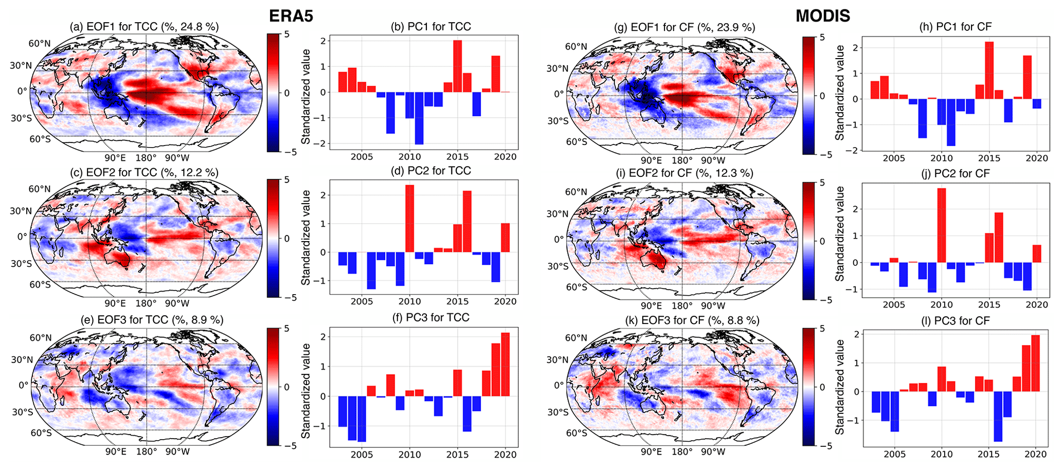
Figure 1 The three dominant EOF modes and their corresponding PCs of the annual cloud coverage anomaly (unit: %) from ERA5 (a–f) and MODIS (g–l) during 2003–2020. (a, g) The scaled leading EOF mode (EOF1, amplified by the standard deviation of its PC). (b, h) The standardized leading PC (PC1, divided by its standard deviation). (c, i) The scaled second EOF mode (EOF2). (d, j) The standardized second PC (PC2). (e, k) The scaled third EOF mode (EOF3). (f, l) The standardized third PC (PC3). The values inside the title's parentheses of panels (a), (c), (e), (g), (i), and (k) indicate the explained variances. The red and blue bars in panels (b), (d), (f), (h), (j), and (l) highlight the positive and negative PC values, respectively.

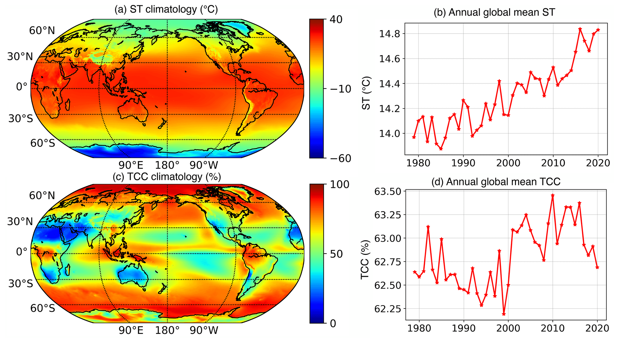
Figure 2 Climatological mean maps and the annual global means (area weighted) of ST (unit: ^∘C) and TCC (unit: %) during 1979–2020. (a) A global map of the climatological mean of ST. (b) Time series of the annual global mean of ST. (c) A global map of the climatological mean of TCC. (d) Time series of the annual global mean of TCC.

2.4 EOF analysis

EOF analysis is a linear decomposition method of multivariate signals that is widely used in meteorology and oceanography (Lorenz, 1956; Preisendorfer and Mobley, 1988), aimed at extracting spatial modes (i.e., patterns) of variability and studying their time evolution. It decomposes any given spatiotemporal field into a set of orthogonal independent EOF modes in the spatial domain whose temporal variations are encoded by the corresponding principal components (PCs). With the proper interpretations, these linearly independent modes can provide useful clues about the physics and dynamics of the investigated system; see e.g., Schnur et al. (1993), Dunkerton (1993), and Dror et al. (2021). More specifically, EOFs and PCs come in pairs and are ordered by the corresponding variance that is explained by each given mode. The number of EOF–PC pairs is here determined by the temporal dimension (42 in total for the annual ST and TCC anomalies considered in this study).

In this study, we used area-weighted data for the EOF analysis of annual ST and TCC anomalies to isolate the main drivers of global surface air temperature and cloud coverage. The area weighting is adopted in order to lessen the contribution of smaller-size grid boxes (Baldwin et al., 2009). Once the EOF analysis is performed on the area-weighted ST and TCC data, the final EOF modes presented in the main text are rescaled by dividing them by the corresponding area weights. The underlying EOF analysis is performed using the Python library, eofs (version 1.4.0, https://github.com/ajdawson/eofs, last access: 15 January 2022 Dawson, 2016).

3 Results

First, to set the stage and to explore modes and sensitivities in the ERA5 TCC dataset as compared to direct measurements, we conducted an area-weighted EOF analysis on annual TCC anomalies and compared it with the observed CF from MODIS; see Fig. 1. To mimic the MODIS CF observations, we resampled ERA5 TCC data to a grid with a horizontal resolution of 1^∘ and considered only a subset of data between 60^∘ N and 60^∘ S during 2003–2020. The subset of ERA5 TCC captures well the leading modes of the MODIS CF and about 60 % of the total variance (Spearman's ρ = 0.77; see Sect. S1 in the Supplement). Figure 1 shows the three dominant EOF modes and PCs of the annual ERA5 TCC and MODIS CF anomalies. The very similar explained variances (as indicated in the title of the EOF panels of Fig. 1), as well as the spatial patterns in EOFs (Spearman's ρ=0.84, 0.83, and 0.75 for the first, second, and third EOFs, respectively) and the temporal evolution of the PCs (Spearman's ρ=0.99, 0.89, and 0.88 for the first, second, and third PCs, respectively), suggest that, although the ERA5 TCC is by definition simulated, the underlying model characteristics and assimilation techniques are able to reproduce essential variations of cloud coverage when compared to observations.

On the strength of this observation, we extend the study period to 1979–2020 based on ERA5 data with a horizontal resolution of 0.25^∘. Figure 2a and c show the geographical distributions of annual mean ST and TCC data. It reveals the nearly uniform temperature gradient towards the poles and the expected patterns of high cloud coverage over the tropics and marine mid-latitudes and the extremely low cloud coverage over the deserts. Figure 2b and d plot the area-weighted global mean ST and TCC data; see Sect. 2. The increasing ST trend represents a clear signature of global warming (Eyring et al., 2021). In contrast, the lack of a consistent trend in TCC suggests that perturbations other than a warming climate might dominate the global TCC variability. For example, the break in the trend around the year 2000 can be attributed to the trend in the maritime clouds over the tropical Atlantic and the western part of tropical Pacific (see Fig. S1 and Sect. S2 in the Supplement) and is likely to be associated with the previously reported phase change of AMO and PDO in the 2000s (Hong et al., 2022).

To identify and isolate the main underlying drivers in the variations, we perform again an area-weighted EOF analysis on annual ST and TCC anomalies. The results reveal spatio-temporal fields sufficient for identifying modes of variability driven by distinct physical processes. By analyzing the PCs' time variability, we are able to find correspondences between the EOF modes and known climate phenomena (Preisendorfer and Mobley, 1988). Notably, unlike EOF modes, physical processes are not necessarily orthogonal, and variations caused by one physical process could be split into different EOF modes, a phenomenon known as signal leakage (Richman, 1986). However, this issue is negligible for the dataset at hand, in particular for the dominant EOF modes of ST and TCC discussed below; see Fig. S2 and Sect. S3 in the Supplement.

To set the stage, we first present our findings for the global surface air temperature. Figure 3 shows the two dominant EOF modes of the annual ST anomaly along with their PCs. Recall that a given PC encodes the temporal variability captured by the corresponding EOF mode, whose spatial features specify, in turn, the magnitude and direction of the PC over each region. For the dataset at hand, the leading EOF mode of ST (EOF1, Fig. 3a) accounts for 32.5 % of the total variance and distills a consistent warming trend (PC1, Fig. 3b) over nearly all continents and most oceans (red shades in Fig. 3a). Its PC evolves almost synchronously with the annual global mean ST (black curve in Fig. 3b).

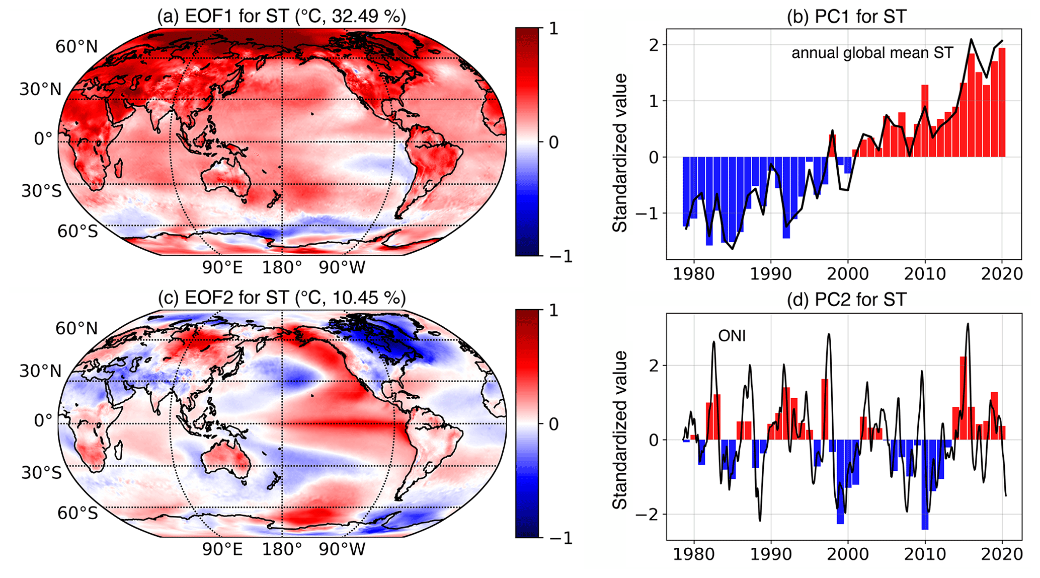
Figure 3 The two dominant EOF modes and their corresponding PCs of the annual ST anomaly (unit: ^∘C) during 1979–2020. (a) The scaled leading EOF mode (EOF1, amplified by the standard deviation of its PC). (b) The standardized leading PC (PC1, divided by its standard deviation). (c) The scaled second EOF mode (EOF2). (d) The standardized second PC (PC2). The values inside the title's parentheses of panels (a) and (c) indicate the explained variances. The black curves in panels (b) and (d) are standardized annual global mean ST and ONI. The red and blue bars in panels (b) and (d) highlight the positive and negative PC values, respectively.

This leading EOF mode reveals some regional features of the recent warming climate, such as the most significant warming being over the Arctic (Serreze and Barry, 2011), the nearly twice-larger warming rate over land compared to over the ocean (Byrne and O'Gorman, 2018), and the feeble warming or even cooling signal over parts of the North Atlantic Ocean, the southeast Pacific Ocean, and the Southern Ocean (Keil et al., 2020; Heede and Fedorov, 2021; Bintanja et al., 2013). These features highlight that regional feedbacks can modify the warming pattern and lead to non-uniform warming.

The second component of ST variations (EOF2, Fig. 3c), accounting here for 10.5 % of the total variance, manifests itself as an ENSO-associated mode. This feature becomes strikingly apparent when comparing its PC (PC2, Fig. 3d) with the ONI, a common measure of ENSO (Glantz and Ramirez, 2020); see the black curve in Fig. 2d and Sect. S4 in the Supplement. An episode of large positive values in PC2 coincides with large positive ONI values, indicating a strong warm phase of ENSO; i.e., El Niño events leading to an unusual increase in sea surface temperature over the central and eastern tropical Pacific Ocean. Analogously, episodes of large negative values for this PC2 coincide with large negative ONI values, corresponding to strong cold phases of ENSO (La Niña events, the cold counterpart of El Niño) (Neelin et al., 1998).

As expected, EOF2 for ST shows strong positive anomalies over the central and eastern tropical Pacific and negative anomalies over the western Pacific. Furthermore, beyond the Pacific Ocean, ST over areas with strong negative (e.g., North America and the adjacent North Atlantic Ocean) and positive (e.g., South Africa, parts of Asia, Australia, and a part of the Southern Ocean) anomalies also closely correlates to ENSO events. These findings are consistent with previous studies (Deser et al., 2010; Davey et al., 2014) and highlight ENSO as an essential driver of the global climate system (Taschetto et al., 2020). Once more, these results ensure that ERA5 performs reasonably well in capturing climate variability during the study period and that the EOF analysis is effective at isolating the warming-associated mode from the influence of other climate perturbations.

Overall, the EOF analysis for ST demonstrates that the global warming trend and ENSO are the dominant factors in surface air temperature variability over the last 42 years.

We turn next to our EOF results of global cloud coverage. Figure 4 presents the two dominant EOF modes and the corresponding PCs of the annual TCC anomaly. The first thing to note is that, similarly to ST findings, a trend and an ENSO-associated mode are identified but in opposite order. The EOF1 for TCC (Fig. 4a) shows an ENSO-associated behavior with its PC (Fig. 4b), evolving almost in perfect synchrony with the ONI. While EOF2 (Fig. 4c) demonstrates a clear trend with its PC (Fig. 4d), which strongly correlates with the annual global mean ST (black curve in Fig. 4d; Spearman's ρ = 0.88, p value = $\mathrm{3.28}\times {\mathrm{10}}^{-\mathrm{14}}$, two-tailed t test).

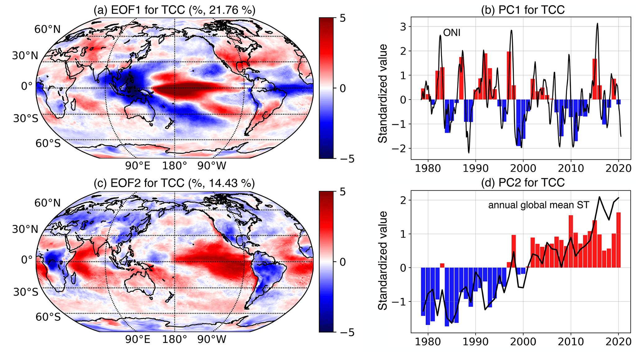
Figure 4 The two dominant EOF modes and their corresponding PCs of the annual TCC anomaly (unit: %) during 1979–2020. (a) The scaled leading EOF mode (EOF1, amplified by the standard deviation of its PC). (b) The standardized leading PC (PC1, divided by its standard deviation). (c) The scaled second EOF mode (EOF2). (d) The standardized second PC (PC2). The values inside the title's parentheses of panels (a) and (c) indicate the explained variances. The black curves in panels (b) and (d) are the standardized ONI and annual global mean ST, respectively. The red and blue bars in panels (b) and (d) highlight the positive and negative PC values, respectively.

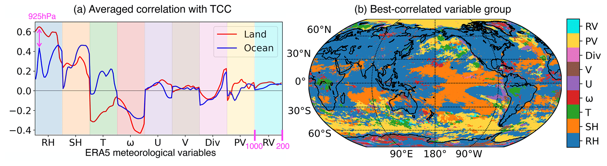
Figure 5 The relationships between annual ERA5 meteorological variables and annual TCC during 1979–2020. (a) Averaged Spearman's ρ (area-TCC-weighted) over land and ocean; ρ values are shown for RH, SH, T, U, V, ω, Div, PV, and RV at 23 standard pressure levels from 1000 to 200 hPa, starting from near the surface on the left part of the section (light-color shades) to the upper atmosphere. (b) Map of the meteorological variables that best correlate with TCC, only Spearman's ρ values that are statistically significant at the level of 0.05 (p value < 0.05, two-tailed t test) are used.

This EOF1 for TCC shows that the global cloud coverage is greatly influenced by ENSO and accounts for 21.8 % of the total variance, similarly to the results shown over the 2003–2020 period; see Fig. 1. It suggests that maritime Southeast Asia and the western Pacific are anti-correlated with the PC and hence the ONI (blue shades in Fig. 4a), meaning the cloud coverage in regions of positive anomalies over the central to eastern Pacific (red shades in Fig. 4a) has a tendency to increase during El Niño years and to decrease during La Niña years. Beyond the Pacific Ocean, the analysis reveals strong negative correlations over the tropical Atlantic Ocean and positive correlations over western Asia, part of South America, the southern United States, and the adjacent North Pacific Ocean. The patterns revealed here are consistent with satellite observations for the ENSO-forced precipitation tendency (Davey et al., 2014). Moreover, they agree well with previous studies showing similar ENSO-associated modes in cloud radiative effects and cloud coverage by means of simulations and corrected satellite records (Yang et al., 2016; Li et al., 2021).

After decoupling the ENSO-associated mode from TCC, an unambiguous trend mode (Fig. 4c) appears. This trend mode in TCC accounts for 14.4 % of the total variance and yields a PC that evolves similarly to the one associated with the ST warming mode; see Fig. 3b). However, unlike the latter, whose warming pattern is expressed throughout the globe, patterns of TCC growth are shown over a major part of the ocean (red shades in Fig. 4c), while patterns corresponding to shrinking TCC occur over most of the continents (blue shades in Fig. 4c). More specifically, the tropical and subtropical oceans exhibit the most significant increasing trends; while, for the continents, South and North America, the Congo Basin, most of Asia, Europe, and the poles exhibit a decreasing trend, the desert areas and the Indian subcontinent tend to display an increasing trend.

By relying on the EOF analysis, we are able to identify an unambiguous signature of the warming climate on global cloud coverage. We explore next the potential thermodynamic drivers that could explain the revealed TCC trend. In that respect, we assess the correlation between each ERA5 meteorological variable (207 in total) and TCC by calculating the corresponding Spearman's ρ for the annual data in Fig. 5. The meteorological variables that are checked here include RH, SH, T, U, V, ω, Div, PV, and RV at 23 standard pressure levels ranging from 1000 to 200 hPa; see Sect. 2.

Figure 5a presents the average correlations over land (LSM > 0.2) and ocean (LSM ≤ 0.2); see Sect. 2. These results show that RH, at most pressure levels, exhibits the strongest correlation with continental TCC, while for maritime TCC, RH and SH yield comparably strong correlations. A previous analysis based on satellite observations and other atmospheric reanalysis datasets obtained similar conclusions (Koren et al., 2010). The geographical distribution of the meteorological variables that best correlate with TCC, shown in Fig. 5b, further highlights RH as the strongest component over almost all continents. Moreover, there is no single variable besides RH that correlates strongly with nearly all continental TCC; see Fig. S3 and Sect. S5 in the Supplement. As for the maritime TCC, it exhibits a diversity of best-correlated variables dominated by RH, SH, and PV. Such correlation differences over land and ocean may be linked to the different atmospheric conditions over land and ocean, as well as to the different dynamics of continental clouds and maritime clouds.

The RH correlation score shows a global peak over land (0.65±0.20) and a local peak over the ocean (0.43±0.22) slightly above the surface (925 hPa, the magenta arrow in Fig. 5a). RH, which, for a given pressure level, is a function of the specific humidity and the temperature, is a key parameter in determining cloud properties. Based on a parcel theory describing convective cloud formation, the low-level RH will determine the likelihood of cloud formation and its extent. Moreover, low-level RH represents a more localized process, while high-level RH values are likely to be affected by processes such as cloud evaporation and long-distance water vapor transport (Bengtsson, 2010).

Therefore, to further explore the links between TCC and RH, we introduce a hybrid RH variable denoted as RH_NS, taking into account the terrestrial topography. RH_NS is defined as RH at 950 hPa over the ocean and at a pressure level of 50 hPa less than the local surface pressure over land; see Sect. 2.

Figure 6a shows the temporal trend in RH_NS for the study duration (1979–2020) using ordinary least-squares-regression analysis (Wells and Krakiwsky, 1971). It shows a consistent decreasing trend in RH_NS over land at a rate of 1 %–2 % of relative humidity per decade, as well as similar spatial patterns in these RH_NS trends compared to those exhibited in the TCC trend mode. The statistically significant RH_NS trends and additional trend analysis of RH_2 m lead to similar conclusions; see Fig. S4 and Sect. S6 in the Supplement. The larger decreasing rate of RH_NS over the continents is expected due to the limited reservoir of water vapor and the larger warming rate over land (see Fig. 3a) and is consistent with previous studies that suggest a decreasing trend in surface air RH over land but only weak changes over the ocean under a warmer climate (e.g., Byrne and O'Gorman, 2018). Figure 6b shows a map of the correlation between RH_NS and TCC, revealing a distinct difference between the high correlation scores for most of the continents (apart from the Sahara) compared to the oceans. The distributions of the correlations (Fig. 6c) show the high and relatively narrow correlation spread over land. Moreover, the global mean correlation of TCC with RH_NS shows the highest score of 0.69±0.18 over land.

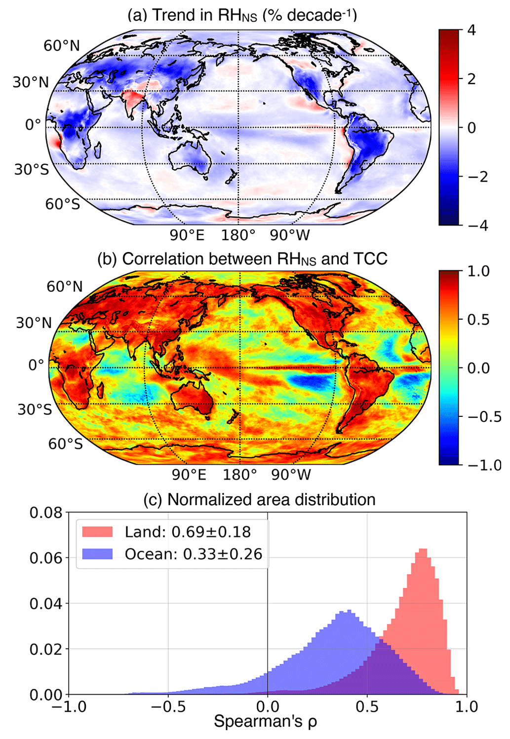
Figure 6 Trends in RH_NS and correlations between annual RH_NS and annual TCC. (a) A map of the temporal trend in annual RH_NS (unit: % per decade⁻¹, where % denotes the absolute rather than the fractional percentage change). (b) A map of Spearman's ρ between RH_NS and TCC. (c) Distribution (area-TCC weighted) of the correlations presented in panel (b) over land and ocean. The distribution's mean and standard deviation are displayed in the box.

4 Discussion

Surface air temperature is likely to be the most explored variable with respect to climate change (Gulev et al., 2021). It is a direct measure of global warming at the most relevant level for most biological systems, and it characterizes the temperature interface between the ocean and land and the atmosphere. As such, it sets boundary conditions for tropospheric processes. Clouds are at the heart of the water cycle and serve as radiation modulators of the atmosphere (Bengtsson, 2010; Stephens et al., 2012). Though the overall effects on the fresh water and radiative budgets depend on the cloud type and properties (Chen et al., 2000; Houze, 2014), the first variable to explore is the horizontal cloud extent, namely what fraction of the sky is cloudy per each region on the globe.

By performing EOF analysis on ERA5 data over 1979–2020, we showed that the two dominant modes of surface air temperature and total cloud coverage can be described as a trend and an ENSO tendency. The order of these modes is flipped; for the surface air temperature, the trend leads the ENSO, while for cloud coverage, the trend follows the ENSO. We used the frequently explored surface air temperature data to set the stage and to demonstrate the rich information that can be drawn from the modes. The temperature analysis reveals a clear trend captured by the leading PC paired with an almost totally red EOF mode (i.e., dominated by positive anomalies) of known regional features (Serreze and Barry, 2011; Byrne and O'Gorman, 2018; Keil et al., 2020; Heede and Fedorov, 2021; Bintanja et al., 2013). The second mode reveals a rich pattern of ENSO weights and signs over the entire globe, highlighting the fact that ENSO is a key driver of the global climate system (Neelin et al., 1998; Taschetto et al., 2020). The cloud coverage analysis shows a clear ENSO mode followed by a trend mode in terms of variance decomposition. The trend mode shows growth in cloud coverage with time over the tropical and subtropical oceans, while a shrinking in cloud coverage is revealed over most non-desert continents.

The reported trends in cloud coverage are consistent with several previous estimations that were based on long-term observations and historical simulations. A few examples are the reported decreasing trend over land as revealed by surface observations (Warren et al., 2007) and the general increasing trend detected over the tropics and eastern subtropics by means of the analysis of satellite observations and historical simulations (Norris and Evan, 2015; Zhou et al., 2016; Norris et al., 2016). Another example is the analysis of the observed liquid water path from the Multi-sensor Advanced Climatology of Liquid Water Path (MAC-LWP) dataset, which showed an increasing trend over most of the oceans (Manaster et al., 2017). However, there are some contradictions between our findings and previously reported satellite observations, which show a decreasing trend over most of the Congo Basin and an increasing trend over most of the northeast tropical Atlantic over the last decades (1983–2009) (Norris and Evan, 2015). Also, some model-based future-climate prediction studies suggest a decrease in marine stratocumulus cloud coverage in warmer climate conditions (Forster et al., 2021; Zelinka et al., 2016). This discrepancy may stem from many reasons, including the uncertainties related to long-term cloud observations (Norris and Evan, 2015), the inaccuracies related to cloud simulations (Stevens and Bony, 2013), the limitations of the ERA5 data (e.g., the quality depends on the assimilated observations) (Hersbach et al., 2020), and the varying global warming patterns in the future (Zhou et al., 2016; Gulev et al., 2021).

The revealed opposing trends of continental and maritime cloud coverage highlight the land–ocean contrast under global warming. The detailed analysis we presented of correlations between annual cloud coverage and thermodynamic variables taken from ERA5 (207 in total) further suggests that the decreasing trend in relative humidity is the main driver of the decreased trend in continental cloud cover. Because of the limited availability of water vapor sources over land, terrestrial clouds are more likely to be humidity limited. Relative humidity measures how far a given specific humidity is from saturation per given temperature and pressure and is, therefore, a fundamental measure of cloud formation. In particular, relative humidity near the surface dictates the initial conditions of a rising air parcel. In a warming climate, over the continents, near-surface relative humidity is expected to decline (Byrne and O'Gorman, 2018) and is likely to affect cloud formation similarly. Over the warming oceans, for which the water vapor reservoir is not limited, enhanced evaporation can supply additional water vapor and hence partly cancel changes in relative humidity due to temperature increasing. Therefore, trends of near-surface relative humidity and their links to cloud coverage over the oceans are less distinct.

Our results have several implications. The more optimistic one is that increased cloud coverage over the central belt of the oceans implies a possible negative cloud feedback to global warming. The total effect will subsequently depend on how the increased cloud coverage is distributed among cloud types and their properties. Nevertheless, as a first approximation, larger subtropical marine stratocumulus decks are likely to cause stronger cooling (Wood, 2012; Zelinka et al., 2017). In contrast, the consistent reduction in cloud coverage over land suggests an additional warming and larger stress on the freshwater supply that is already in shortage in many regions around the globe (Oki and Kanae, 2006). Moreover, such a contrast in cloud trends between land and ocean (Fig. 4c) suggests changes in the radiative energy partitioning between the two media that could be responsible for igniting additional feedbacks and changes in the atmospheric circulation.