A new process-based and scale-aware desert dust emission scheme for global climate models – Part I: Description and evaluation against inverse modeling emissions

Desert dust accounts for most of the atmosphere's aerosol burden by mass and produces numerous important impacts on the Earth system. However, current global climate models (GCMs) and land-surface models (LSMs) struggle to accurately represent key dust emission processes, in part because of inadequate representations of soil particle sizes that affect the dust emission threshold, surface roughness elements that absorb wind momentum, and boundary-layer characteristics that control wind fluctuations. Furthermore, because dust emission is driven by small-scale (∼ 1 km or smaller) processes, simulating the global cycle of desert dust in GCMs with coarse horizontal resolutions (∼ 100 km) presents a fundamental challenge. This representation problem is exacerbated by dust emission fluxes scaling nonlinearly with wind speed above a threshold wind speed that is sensitive to land-surface characteristics. Here, we address these fundamental problems underlying the simulation of dust emissions in GCMs and LSMs by developing improved descriptions of (1) the effect of soil texture on the dust emission threshold, (2) the effects of nonerodible roughness elements (both rocks and green vegetation) on the surface wind stress, and (3) the effects of boundary-layer turbulence on driving intermittent dust emissions. We then use the resulting revised dust emission parameterization to simulate global dust emissions in a standalone model forced by reanalysis meteorology and land-surface fields. We further propose (4) a simple methodology to rescale lower-resolution dust emission simulations to match the spatial variability of higher-resolution emission simulations in GCMs. The resulting dust emission simulation shows substantially improved agreement against regional dust emissions observationally constrained by inverse modeling. We thus find that our revised dust emission parameterization can substantially improve dust emission simulations in GCMs and LSMs.

1 Introduction

Desert dust accounts for more than half of the atmospheric mass loading of particulate matter (PM) (Kinne et al., 2006; Kok et al., 2017) and produces a wide range of important impacts on multiple components of the Earth system (Shao et al., 2011a; Kok et al., 2023). Like other aerosols, dust changes Earth's radiative budget and atmospheric dynamics directly by scattering and absorbing radiation (Sokolik and Toon, 1996; Miller and Tegen, 1998) and indirectly by mediating cloud formation (Rosenfeld et al., 2001; Shi and Liu, 2019; McGraw et al., 2020; Froyd et al., 2022). These dust–radiation interactions and dust–cloud interactions also drive day-to-day variability in large-scale circulation patterns and local weather events such as monsoons and rainfall (Jin et al., 2021; Parajuli et al., 2022). Dust further impacts biogeochemistry by delivering nutrients such as iron and phosphorus to ocean and land ecosystems (Mahowald et al., 2010; Hamilton et al., 2020).

In recent decades, modelers have made substantial progress in developing various parameterizations for the main dust cycle processes including emission (e.g., Shao et al., 1993; Marticorena and Bergametti, 1995; Marticorena et al., 1997; Tegen and Fung, 1995; Klose and Shao, 2013), advection (e.g., Prospero, 1999; Lin, 2004; Van der Does et al., 2018), deposition (e.g., Barth et al., 2000; Liu et al., 2001; Zhang et al., 2001; Petroff and Zhang, 2010) and its biogeochemical effects (e.g., Jickells et al., 2005; Mahowald et al., 2005, 2010; Hamilton et al., 2020), optics (e.g., Sokolik and Golitsyn, 1993; Linke et al., 2006; Adebiyi and Kok, 2020), and radiative effects (e.g., Di Biagio et al., 2020; Li et al., 2021). Despite substantial progress in dust modeling, current global climate models (GCMs) and Earth system models (ESMs) still struggle to adequately simulate the dust cycle, which impedes an accurate assessment of dust impacts (Huneeus et al., 2011; Wu et al., 2020; Zhao et al., 2022). For instance, model simulations still show large discrepancies when compared against observations of the spatial and temporal characteristics of the dust cycle, including dust emission (Kok et al., 2014a; Pierre et al., 2014a), dust PM concentration (Wu et al., 2019; Pu et al., 2020; Li et al., 2022), dust aerosol optical depth (DAOD or DOD) (Ridley et al., 2012; Kok et al., 2014b; Pu and Ginoux, 2018; Parajuli et al., 2019), dust deposition (Ginoux et al., 2001; Albani et al., 2014; Kok et al., 2014b; Li et al., 2022), and dust size distributions (Parajuli et al., 2019; Adebiyi and Kok, 2020; Li et al., 2022). Also, models struggle to capture the observed interannual and decadal variability of dust (Ridley et al., 2014; Smith et al., 2017; Evan, 2018; Kok et al., 2018) and the sensitivity of dust to climate changes (Evan, 2018; Kok et al., 2018). An improved quantification of dust impacts on the Earth system thus requires improvements on how dust is simulated in models.

One key piece of physics that models struggle to parameterize is the dust emission threshold. The dust emission threshold u_∗t is defined as the threshold wind stress/speed above which winds initiate, or below which winds cease, the lifting of sand particles whose impacts on the soil surface emit dust aerosols (Kok et al., 2012; Comola et al., 2019b). The dust emission threshold is a function of soil properties and atmospheric conditions like particle size distribution, soil moisture, and air density. There are various reasons for the inadequate parameterization of the dust emission threshold. First, many models assume a globally constant soil particle size in calculating a spatially varying dust emission threshold (Zender et al., 2003a; Darmenova et al., 2009; Kok et al., 2014b), whereas the actual soil particle size is likely a function of space and time and could depend on soil properties, such as texture, pH, and organic matter content, since these variables modulate the cohesion between soil particles (Webb et al., 2016). Some models proposed that soil particle sizes are related to the soil texture and therefore represent the soil particle size as a global map (Tegen et al., 2002; Darmenova et al., 2009; Menut et al., 2013; Klose et al., 2021), but these maps either have not yet been thoroughly validated against observations or are based upon extrapolation of a limited number of observations. Second, most current models use the fluid threshold (also named static threshold or initiation threshold) above which saltation is initiated as the dust emission threshold, but it is well known that dust emission is governed by both the larger fluid threshold and the smaller impact threshold (also named dynamic threshold or cessation threshold) below which saltation is terminated (Bagnold, 1941; Shao, 2008; Martin and Kok, 2018; Comola et al., 2019a, b; Pähtz et al., 2020). Moreover, dust emission is a nonlinear process (i.e., it varies with the wind speed to the second to fifth power, per Kok et al., 2014a), and the emission flux is particularly sensitive to the magnitude of the emission threshold (Kawai et al., 2021). Thus, land-surface models (LSMs) within GCMs and ESMs need to parameterize the emission threshold correctly to get an adequate spatiotemporal variability of the modeled atmospheric dust.

The second key dust emission physics that LSMs struggle to represent is the partitioning of the wind stress. Wind drag is partitioned into the part absorbed by surface roughness elements (mainly rocks and plants) and the part exerted on the bare soil that drives dust emissions. This drag partitioning effect is modeled by several dynamical schemes (Raupach et al., 1993; Marticorena and Bergametti, 1995; Okin, 2008), and it is accounted for in some models (LeGrand et al., 2019; Klose et al., 2021; Tai et al., 2021) but not others (e.g., Kok et al., 2014b; Evans et al., 2016). One major challenge in modeling drag partition is to quantify the abundance of rocks (which includes rocks, pebbles, and gravel in this study) and their corresponding partition effect, because there are few measurements of rock roughness. To cope with this issue, studies have used in situ and/or remote sensing scatterometer measurements to quantify the small-scale land-surface roughness (e.g., Greeley et al., 1997; Roujean et al., 1997; Marticorena et al., 2004; Prigent et al., 2005, 2012), especially over arid desert regions over which rocks, pebbles, and gravel dominate the roughness. However, with a few recent notable exceptions that attempted to represent the roughness effects of both rocks and vegetation (e.g., Darmenova et al., 2009; Foroutan et al., 2017; Klose et al., 2021), studies often omitted the drag partition effect either due to vegetation (e.g., Menut et al., 2013) or due to rocks (e.g., Wu et al., 2016; LeGrand et al., 2019; Tai et al., 2021). To resolve these issues, we propose a new approach that combines the drag partition effects of both elements, leveraging satellite scatterometer measurements to quantify the surface rock roughness and using observable vegetation and land-surface variables to quantify the surface vegetation roughness.

The third key piece of fundamental dust emission physics not accounted for by many models is the effect of turbulence-driven high-frequency wind variability on dust emissions. Most current GCMs assume a constant wind speed (and thus a constant emission flux) within the relatively large model time step, e.g., 30 min (e.g., Rahimi et al., 2019; Dunne et al., 2020). However, in reality, high-frequency turbulent fluctuations cause the wind speed to fluctuate within a time step (from seconds to minutes). Because dust emissions scale nonlinearly with wind speed, this causes highly uneven and fluctuating dust emission fluxes (Durán et al., 2011). Even more importantly, turbulent wind fluctuations can sweep across the dust emission threshold multiple times and shut off dust emissions intermittently within one model time step, resulting in strong dust emission intermittency (Comola et al., 2019b). Even regional climate models (RCMs), which typically use a smaller time step (e.g., <1 min), do not resolve turbulence unless they are run in the computationally expensive large-eddy-simulation (LES) mode (e.g., WRF–LES). Omitting turbulence by GCMs and RCMs thus causes either an overestimate or an underestimate of dust emissions, especially over marginal source regions where winds fluctuate around the high emission threshold, as models do not account for the cessations or initiations of dust emissions due to turbulent fluctuations. To account for the instantaneous wind fluctuations, a dynamical approach is to derive a probability density function (PDF) for the instantaneous momentum flux using LES, which is then used for quantifying instantaneous dust emission fluctuations (Klose and Shao, 2012; Klose et al., 2014). A parameterization approach is to use the Monin–Obukhov similarity theory (MOST) to relate the standard deviation of the instantaneous wind to the boundary-layer dynamical variables (Comola et al., 2019b). In this study, we will account for turbulent dust emissions by following Comola et al. (2019b), which showed significant improvements in representing the small-magnitude saltation and dust fluxes that are particularly important over marginal source regions.

In addition to these issues of models missing some of the fundamental physics of dust emission, a central issue in modeling the global dust cycle is that dust emissions are grid-resolution-dependent because of the nonlinear dependence of dust emissions to meteorological fields and land-surface variables. Since dust emission varies nonlinearly with wind speed and has an even more complex relation to the soil moisture (Gillette and Passi, 1988; Fécan et al., 1999; Shao, 2001; Kok et al., 2014a), the total regional and global emissions can vary significantly with grid resolution (Ridley et al., 2013; Meng et al., 2021). For instance, modeled emissions were found to increase by ∼ 29 % from a 1^∘ × 1^∘ to 0.25^∘  × 0.25^∘ resolution (Ridley et al., 2013; Feng et al., 2022). As a consequence, GCMs and ESMs often need to tune emissions separately for different grid resolutions to match observational dust budgets (Ginoux et al., 2001; Zender et al., 2003a; Albani et al., 2014; Kok et al., 2014b; Chappell et al., 2021). This issue occurs because current GCM grid sizes of ∼ 1^∘ or 100 km cannot resolve the spatial scales of ∼ 1 m to ∼ 1 km over which soil properties and wind speeds change (Ridley et al., 2013). When adopting coarse grid resolutions, coarser modeled meteorological fields (for GCMs) or spatially averaged input meteorological fields (for chemical transport models or CTMs) will smooth out the local wind extrema, possibly causing wind speeds to fall below the dust emission threshold. As a result, the coarse modeled winds usually result in strong GCM emissions underestimations (Ridley et al., 2013). The same smoothing problem also occurs for soil moisture for instance, with its maxima smoothed out leading to an overestimation of dust emissions. Thus, although some GCMs and ESMs recently implemented more physical schemes (Zhao et al., 2022), their inability to resolve the small scales still causes challenges for capturing the accurate spatial distributions of dust emissions (Meng et al., 2021). For the same reason, GCMs tend to neglect small-scale emissions over marginal source regions. In this study, we will analyze the scale dependence of our dust emission scheme given specific input datasets and propose a method of upscaling the coarse dust emissions to alleviate the scale-dependence problem.

To tackle the above problems and improve simulations of the global dust cycle, we propose a new emission scheme for global models that includes key dust emission physics missing from current models. Specifically, we (1) account for the effects of the soil particle size distribution (PSD) on the dust emission threshold, (2) draw on satellite data and physically explicit models to account for wind momentum absorption by both rocks and vegetation, and (3) account for turbulence-driven intermittency in dust emission fluxes. After we review current dust emission schemes in Sect. 2, we present our new scheme in Sect. 3. In Sect. 4, we code the new dust emission scheme as a standalone sandbox model (see Sect. 2.4) and examine the resulting spatiotemporal variability of the new dust emissions. We then examine the grid-scale dependence of dust emissions and derive a correction map for coarser dust emission simulations to correct their spatial variability to high-resolution simulations. Sections 5 and 6 discuss and summarize the main findings of this paper. In our companion paper (Leung et al., 2023b), we will implement this new scheme in the state-of-the-art Community Earth System Model version 2 (CESM2) and evaluates its performance against observations.

2 Current dust emission schemes and their input variables

This section provides a basic review of current GCM's dust emission schemes and their required input meteorological variables. Broadly speaking, dust emission schemes consist of a parameterization of the dust emission threshold (Sect. 2.1); a parameterization of the reduction of the wind drag on the bare soil surface due to momentum absorption by surface roughness elements (Sect. 2.2); and a parameterization of dust emission flux given wind speed, threshold wind speed, and drag absorption (Sect. 2.3). We will develop an improved emission scheme for GCMs in Sect. 3 by improving upon each of these three core ingredients of dust emission schemes. We also provide a brief description of meteorological data used for computing the dust emission schemes in Sect. 2.4.

2.1 Parameterization of the dust emission thresholds

There have been extensive studies on the dust emission threshold u_∗t, defined as the wind speed or drag that corresponds to the initiation or cessation of dust emission. Dust emission is caused by saltation, a process by which sand particles (geometric diameter >63 µm) on the surface are lifted by wind drag into the airstream (known as aerodynamic entrainment) and undergo ballistic trajectories (Anderson, 1989; Kok et al., 2012). The minimum wind friction velocity u_∗ required for initiating saltation through aerodynamic entrainment is called the fluid threshold u_∗ft (McKenna Neuman and Sanderson, 2008). Once saltation is initiated, a smaller u_∗ is needed to maintain saltation because saltation bombardment (saltating particles impacting on the granular bed) can create further saltation, which is more efficient than creating saltation solely through the wind drag. Saltation will be maintained at a slightly smaller u_∗ called the impact threshold u_∗it (Bagnold, 1941; Martin and Kok, 2018). The ratio $u_{\ast \mathrm{it}}/u_{\ast \mathrm{ft}}$ is about 0.8–0.85 for loose dry sand and less for soils with other sources of cohesion (e.g., moisture, organic matter), because cohesion rapidly increases u_∗ft, but low-to-moderate levels of cohesion do not increase u_∗it as indicated by numerical simulations (Comola et al., 2019a; Ralaiarisoa et al., 2022). It follows that dust emission can occur below u_∗ft, especially in marginal dust source regions with high soil moisture for which u_∗it can be much smaller than u_∗ft. u_∗t is thus a general concept comprised of both u_∗ft and u_∗it. However, u_∗it is not currently accounted for in most current GCMs, which simply use u_∗ft as u_∗t.

One challenge in parameterizing u_∗ft and u_∗it lies in the representation of the effect of the soil particle size D_p on both thresholds. These two thresholds are mainly governed by soil particle diameter D_p, air density ρ_a, and soil moisture w (Greeley et al., 1997; Shao and Lu, 2000). Although there are multiple data sources of globally gridded products for ρ_a and w, there are relatively few efforts on obtaining globally gridded D_p, since there are no methods for satellites to observe and derive surface D_p observations. With few comprehensive field studies of saltation dynamics over polydisperse soils, past saltation studies either assumed that particles of different sizes saltate independently of each other (Marticorena and Bergametti, 1995; Shao et al., 1996; Alfaro and Gomes, 2001; Zender et al., 2003a) or assumed that a single grain size (e.g., the median) could be used to represent the whole PSD of the soil bed (Elbelrhiti et al., 2005; Andreotti et al., 2010). The dispute of whether the assumption of “independent” saltation (Shao, 2008) or “representative” saltation (Claudin and Andreotti, 2006) is more appropriate was informed by Martin and Kok (2019), who showed that modeling the threshold using a single particle size (representative saltation) is more realistic than assuming no interactions between saltation of different particle sizes. They argued that the median particle diameter ${\stackrel{\mathrm{‾}}{D}}_{\mathrm{p}}$ of the PSD should be used for calculating the threshold of a mixed soil, and the emission should then be calculated for the whole soil bed using the median instead of using a spectral/independent approach of calculating emissions of different particle sizes separately.

To model u_∗ft, current models assume that u_∗ft is mainly dependent on the soil PSD and soil moisture (Iversen and White, 1982; Marticorena and Bergametti, 1995; Zender et al., 2003a):

$$\begin{array}{}\text{(1)}& u_{\ast \mathrm{ft}}=u_{\ast \mathrm{ft}\mathrm{0}}(D_{\mathrm{p}},{\mathit{\rho }}_{\mathrm{a}})f_{\mathrm{m}}\left(w\right),\end{array}$$

where u_∗ft0 is the “dry” fluid threshold friction velocity (in m s⁻¹) on a smooth and bare surface as a function of air density ${\mathit{\rho }}_{\mathrm{a}}(\mathrm{long},\mathrm{lat},t)$ (longitude, latitude, time) and D_p(long,lat), which in this study will be the median diameter ${\stackrel{\mathrm{‾}}{D}}_{\mathrm{p}}$ of a polydispersed, mixed soil PSD. f_m is the correction factor for the presence of soil moisture $w(\mathrm{long},\mathrm{lat},t)$; f_m≥1, such that soil moisture protects soil particles from being lifted. u_∗ft is the “wet” fluid threshold accounting for the moisture effect. Other factors can also affect u_∗ft, such as salt concentration, organic matter, electrostatic effects, and surface crusts, but they are not included in most studies because they are not well understood and modeled (Shao et al., 2011; Foroutan et al., 2017).

u_∗ft0 is parameterized by considering the balance between aerodynamic drag and lift against gravity and interparticle cohesion on a soil particle. The Shao and Lu (2000) (hereafter S&L00) scheme derived a simple solution to the force balance (also see Kok et al., 2012), assuming that the cohesive force is proportional to particle size. Using wind tunnel measurements (e.g., Greeley and Iversen, 1985), they obtained the following equation with fitting parameters:

$$\begin{array}{}\text{(2)}& u_{\ast \mathrm{ft}\mathrm{0}}=\sqrt{A({\mathit{\rho }}_{\mathrm{p}}g{D}_{\mathrm{p}}+\mathit{\gamma }/D_{\mathrm{p}})}{\mathit{\rho }}_{\mathrm{a}}^{-\mathrm{0.5}},\end{array}$$

where g=9.81 m s⁻² is the gravitational acceleration, ρ_p = 2650 kg m⁻³ is the typical soil particle density, ρ_a is in kg m⁻³, and A=0.0123 and $\mathit{\gamma }=\mathrm{1.65}\times {\mathrm{10}}^{-\mathrm{4}}$ kg s⁻² are empirical constants accounting for the aerodynamic forces and interparticle forces, respectively. Assuming an air density ρ_a=1.225 kg m⁻³, Eq. (2) will yield the smallest u_∗ft0 of 0.21 m s⁻¹ at D_p=80 µm. For larger sizes, the particles are heavier to lift; for smaller sizes, the particles are more strongly bound by interparticle forces.

An alternative parameterization for u_∗ft0 is the Iversen and White (1982) scheme (hereafter I&W82). They derived a similar solution as S&L00 but further considered the effects of soil particle size to the airflows, characterized by the particle Reynolds number Re_p. I&W82 calculates $u_{\ast \mathrm{ft}\mathrm{0}}=u_{\ast \mathrm{ft}\mathrm{0}}\left({\mathit{\rho }}_{\mathrm{p}},{\mathit{\rho }}_{\mathrm{a}},g,D_{\mathrm{p}},{\mathrm{Re}}_{\mathrm{p}}\right)$ in a similar form to S&L00 (see the detailed solution in I&W82 or Kok et al., 2012), with

$$\begin{array}{}\text{(3)}& {\mathrm{Re}}_{\mathrm{p}}=u_{\ast \mathrm{ft}\mathrm{0}}{D}_{\mathrm{p}}/\mathit{\nu },\end{array}$$

where ν is the kinematic viscosity of air. Since u_∗ft0 is a function of Re_p, which itself is a function of u_∗ft0, u_∗ft0 is an implicit function of itself, and the calculation needs to be iterated a few times given ρ_a and D_p in calculation.

Regardless of whether S&L00 or I&W82 is used, different models make different assumptions for soil particle sizes D_p, including a globally constant value (e.g., Zender et al., 2003a), a function of soil texture (e.g., Menut et al., 2013), or other forms. For instance, the Community Land Model (CLM), the land component of CESM, uses a global optimal soil diameter of D_p=75 µm for the threshold calculation following Zender et al. (2003a) (Oleson et al., 2013; also see the latest version of CLM5.0 technical note on https://escomp.github.io/ctsm-docs/versions/release-clm5.0/html/tech_note/index.html, last access: 3 October 2022). Thus u_∗ft0 becomes solely a function of ρ_a in CESM (e.g., $u_{\ast \mathrm{ft}\mathrm{0}}=\mathrm{0.21}\mathrm{m}{\mathrm{s}}^{-\mathrm{1}}$ for ρ_a=1.225 kg m⁻³ at D_p=75 µm).

Most models parameterize the effect of soil moisture f_m on u_∗ft following Fécan et al. (1999):

4a$$\begin{array}{}\text{(4a)}& {\displaystyle }{f}_{\mathrm{m}}=\sqrt{\mathrm{1}+\mathrm{1.21}{\left(w-w_{\mathrm{t}}\right)}^{\mathrm{0.68}}}\mathrm{for}w>w_{\mathrm{t}}\end{array}$$

4b$$\begin{array}{}\text{(4b)}& {\displaystyle }\begin{array}{rl}{w}_{\mathrm{t}}& =a(\mathrm{17}{f}_{\mathrm{clay}}+\mathrm{14}{f}_{\mathrm{clay}}^{\mathrm{2}})\\ & =a\left(\mathrm{0.17}\left(\mathit{\%}\mathrm{clay}\right)+\mathrm{0.0014}{\left(\mathit{\%}\mathrm{clay}\right)}^{\mathrm{2}}\right),\end{array}\end{array}$$

where $w(\mathrm{long},\mathrm{lat},t)$ is the gravimetric soil moisture (kg kg⁻¹) in the shallowest soil layer (see Sect. S1 and Fig. S1 for the relation between volumetric and gravimetric moisture); w_t(long,lat) is the threshold gravimetric water content above which u_∗ft increases; f_clay(long,lat) is the fraction of clay content in the topmost layer of soil between zero and one; %clay=100f_clay is the corresponding clay percentage; and a, a tunable constant usually of order 1, was introduced by Zender et al. (2003a) to account for the mismatch in the small scales for which Fécan et al. (1999) obtained their parameterization and the large scales on which it is used in climate models (e.g., Zender et al., 2003a; Mokhtari et al., 2012; Kok et al., 2014b). w_t increases with soil clay content as water adsorbs onto clay such that more moisture is needed to enhance u_∗ft.

Another essential dust emission threshold for this study is the dynamic or impact threshold u_∗it, which is the lowest wind speed or stress to maintain saltation (Kok et al., 2012; Comola et al., 2019b):

$$\begin{array}{}\text{(5)}& u_{\ast \mathrm{it}}=B_{\mathrm{it}}{u}_{\ast \mathrm{ft}\mathrm{0}},\end{array}$$

where B_it=0.82 is approximately constant with soil properties and particle size (Bagnold, 1937; Kok et al., 2012). Eqs. (2)–(5) imply that $u_{\ast \mathrm{ft}}\ge u_{\ast \mathrm{ft}\mathrm{0}}>u_{\ast \mathrm{it}}$ and that u_∗ft and u_∗it have different spatiotemporal variability. Also, the difference between u_∗ft and u_∗it could be much larger in nonarid regions because f_m is much larger than one. In this study, we propose that dust emission models should use u_∗it instead of u_∗ft for dust emission equations (e.g., Eqs. 10 and 13), which will cause substantial changes in the simulated spatiotemporal variability of dust emission (see Sect. 4.1). This is needed to allow dust emission when the u_∗ is intermediate between u_∗it and u_∗ft, which is especially common in marginal dust source regions. Additionally, this is more physically correct as the dust emission threshold is the minimum friction velocity at which the saltation and dust emission fluxes are nonzero, which is true at u_∗it but not true at u_∗ft (Martin and Kok, 2018; Comola et al., 2019b; Pähtz et al., 2020).

2.2 Parameterization of drag partition effects

Apart from the dust emission threshold, another essential parameter for determining the dust emission flux is the wind drag partition effect, F_eff, due to the existence of land-surface roughness elements covering the desert surfaces (Raupach, 1992; Marticorena and Bergametti, 1995). It is crucial to account for this effect for accurately simulating the magnitude and spatial pattern of dust emissions. Many past modeling studies treated this effect as increasing the dust emission threshold u_∗ft (e.g., Raupach, 1992; Marticorena and Bergametti, 1995; Darmenova et al., 2009; Menut et al., 2013), such that the relation is expressed as (Raupach et al., 1993; Marticorena and Bergametti, 1995; Marticorena et al., 1997, 2006; Foroutan et al., 2017; Webb et al., 2020)

$$\begin{array}{}\text{(6a)}& u_{\ast \mathrm{ft}}=u_{\ast \mathrm{ft}\mathrm{0}}(D_{\mathrm{p}},{\mathit{\rho }}_a)f_{\mathrm{m}}\left(w\right)/F_{\mathrm{eff}},\end{array}$$

where F_eff<1 when roughness elements are present, such that roughness elements increase u_∗ft and decrease the dust emission. However, this approach is physically incorrect because roughness elements reduce the wind stress exerted on the bare soil and do not increase the forces resisting particle lifting that determine u_∗ft (Kok et al., 2014a; Webb et al., 2020). As a consequence, Webb et al. (2020) showed that dust models using Eq. (6a) will overestimate the dust emission flux compared to those using Eq. (6b). A correct emission modeling approach should instead combine Eq. (1) for u_∗ft with the effect of drag partition F_eff to u_∗:

$$\begin{array}{}\text{(6b)}& u_{\ast \mathrm{s}}=u_{\ast }{F}_{\mathrm{eff}},\end{array}$$

where u_∗s is called the soil surface friction velocity (Webb et al., 2020). Dust emissions should thus be a function of u_∗s instead of u_∗.

There are different schools of drag partition schemes. A major school of drag partition parameterization originated from Arya (1975) and later Marticorena and Bergametti (1995) (hereafter M&B95), who primarily used the roughness length z₀ to quantify roughness. Because of the large differences in the length scales between mountains/orography, rocks, and plants, as well as down to soil particles, Menut et al. (2013) distinguished three distinct roughness lengths describing different sizes of roughness. First, the aerodynamic momentum roughness length z_0m mainly represents roughness due to large-scale orography, forests, and/or urbanization (with sizes of 10–10³ m) with values ranging from ∼ 1 cm to 1 m (Menut et al., 2013). Second, the aeolian roughness length z_0a quantifies the roughness due to smaller elements such as rocks and vegetation, with a typical order of magnitude of 10⁻³ to 10 cm (Prigent et al., 2005; Prigent et al., 2012). z_0a is the relevant roughness length that informs the partition of the wind stress when considering the near-surface (∼ 1 m) flows in which saltation occurs. Third, the smooth roughness length z_0s quantifies the roughness of a bed of fine soil particles in the absence of roughness elements. z_0s characterizes the roughness of mobile, erodible soil particles over an exposed surface. z_0s is directly related to the particle diameter D_p by (Nikuradse, 1950; Sherman, 1992; Pierre et al., 2014b)

$$\begin{array}{}\text{(7)}& z_{\mathrm{0}\mathrm{s}}=\mathrm{2}{\mathrm{D}}_{\mathrm{p}}/\mathrm{30}.\end{array}$$

M&B95 proposed their drag partition scheme by arguing that behind a roughness element (obstacle), an internal boundary layer (IBL) grows, and the wind within the IBL follows the log law of the wall as a function of u_∗s and the local roughness length z_0s. They then pointed out that without the obstacle, the planetary-boundary-layer (PBL) wind profile would follow the log law as a function of u_∗ and z_0a. By arguing that the two wind speeds must be equal at the IBL height δ, they derived F_eff as a function of z_0a and z_0s:

$$\begin{array}{}\text{(8)}& F_{\mathrm{eff}}=\mathrm{1}-{\displaystyle \frac{\ln \left(\frac{z_{\mathrm{0}\mathrm{a}}}{z_{\mathrm{0}\mathrm{s}}}\right)}{\ln \left(\frac{\mathit{\delta }}{z_{\mathrm{0}\mathrm{s}}}\right)}}.\end{array}$$

Later studies improved this equation based on more observations for calibrating several parameters (MacKinnon et al., 2004; King et al., 2005; Darmenova et al., 2009; see Eq. 15 in Sect. 3.2). Historically this scheme has been employed by Marticorena and others to represent the roughness due to rocks (e.g., Marticorena et al., 1997; Darmenova et al., 2009; Menut et al., 2013).

Another major school of drag partition parameterization originated from Raupach (1992) and Raupach et al. (1993) (hereafter R93), which primarily used the roughness density λ to quantify roughness. λ is defined as the total frontal area of roughness elements divided by the area of land $A:\mathit{\lambda }=\mathrm{nhb}/A$, where h and b are the obstacle height and width, and n is the number of obstacles within the area. Knowing the geometric and aerodynamic properties of the roughness elements, R93 showed that the drag force of the exposed area ${\mathit{\tau }}_{\mathrm{S}}^{\prime }$ is related to the total drag force τ, given λ, the roughness-element basal area-to-frontal area ratio σ, and the ratio of the roughness element-to-surface drag coefficient β:

$$\begin{array}{}\text{(9a)}& {\displaystyle \frac{{\mathit{\tau }}_{\mathrm{S}}^{\prime }}{\mathit{\tau }}}={\displaystyle \frac{\mathrm{1}}{(\mathrm{1}-m\mathit{\sigma }\mathit{\lambda })(\mathrm{1}+m\mathit{\beta }\mathit{\lambda })}},\end{array}$$

where m is a geometric parameter to account for the spatial variability of ${\mathit{\tau }}_{\mathrm{S}}^{\prime }$ on the erodible surface. Raupach then applied this ratio to the dust emission threshold (per Eq. 6a).

Many later studies used the R93 parameterization for plants (specifically shrubs) with prescribed σ, m, and β (Darmenova et al., 2009; Xi and Sokolik, 2015). λ, however, is related to the abundance of obstacles and is thus spatially variable, and thus far there are no globally gridded datasets of λ available. Most studies thus related grid-scale λ to other grid-scale properties; for instance, Shao et al. (1996) linked λ to the vegetation cover fraction f_v using in situ observations:

$$\begin{array}{}\text{(9b)}& \mathit{\lambda }=c_{\mathit{\lambda }}\ln \left(\mathrm{1}-f_{\mathrm{v}}\right),\end{array}$$

where c_λ is a proportionality constant. Gridded λ could thus be obtained from gridded satellite retrievals of vegetation cover (Gutman and Ignatov, 1998; Wu et al., 2016; Foroutan et al., 2017) or parameterized as a function of other gridded land-surface variables such as the leaf area index (LAI) (e.g., Klose et al., 2021). Later studies have attempted to improve Raupach's parameterization, and newer schemes relating F_eff and λ have emerged (e.g., Okin, 2008).

Many previous modeling studies have not accounted for the drag partition effects of both rocks and vegetation on dust emissions (e.g., Ginoux et al., 2001; Tegen et al., 2002; Zender et al., 2003a; Kok et al., 2014b). Many past studies either accounted for only the drag partitioning by rocks (e.g., Marticorena et al., 2006; Menut et al., 2013) or by vegetation (e.g., Shao et al., 2011b; Wu et al., 2016), mainly because it is very challenging to use proxies of both rocks and vegetation in either the M&B95 or R93 scheme. For instance, R93 was historically mostly used for modeling vegetation but not rock drag partitioning because there was no dataset of the λ due to rocks. Similarly, vegetation roughness is historically mostly represented by λ rather than z_0a, so there is no globally gridded z_0a observations for vegetation that can be fed into the M&B95 scheme. Some modeling studies (e.g., Klose et al., 2021) generated globally gridded vegetation z_0a by relating plant λ with z_0a (e.g., Minvielle et al., 2003; Shao and Yang, 2005; Marticorena et al., 2006; Foroutan et al., 2017; Klose et al., 2021), but these studies all found slightly different relations between λ with z_0a, and often the in situ obstacle height h is required by the relation. It is thus very challenging to model vegetation drag partitioning using M&B95 by converting λ to z_0a when globally gridded h (short vegetation height but not canopy height) is mostly unknown in GCMs or possesses strong subgrid variability. A more recent approach quantifies surface roughness by detecting the shadow (sheltered area) behind a roughness element using satellite-derived albedo (Chappell and Webb, 2016). This approach could potentially capture both rock and vegetation roughness and was also employed by later dust modeling studies (e.g., LeGrand et al., 2023). To our knowledge, there are a few studies that attempted to represent both rock and vegetation roughness in one drag partition scheme (e.g., Darmenova et al., 2009; Foroutan et al., 2017; Klose et al., 2021), but all were affected by important limitations (see Sect. S2 for a discussion on their approaches). In Sect. 3.2, we will propose a novel approach that incorporates roughnesses of both rocks and plants and equally respects the z_0a and λ from both schools of drag partition parameterizations, quantifying the drag partitions of rocks and plants into one hybrid drag partition factor F_eff.

2.3 Parameterization of dust emission flux

There are multiple available dust emission equations (e.g., Gillette and Passi, 1988; Shao et al., 1996; Alfaro and Gomes, 2001; Ginoux et al., 2001; Tegen et al., 2002; Zender et al., 2003a; Shao, 2004; Kok et al., 2014b; Evans et al., 2016; and more) implemented in GCMs and ESMs to calculate dust emission fluxes. For example, the Zender et al. (2003a) scheme (hereafter Z03) is based on the Marticorena and Bergametti (1995) dust emission equation and is a popular dust emission scheme adopted by many GCMs (e.g., Miller et al., 2004; Oleson et al., 2013; Meng et al., 2021). Z03 calculates dust emission as follows:

$$\begin{array}{}\text{(10)}& \begin{array}{rl}{F}_{\mathrm{d}}& ={\mathrm{STC}}_{\mathrm{MB}}\mathit{\phi }{f}_{\mathrm{bare}}{\displaystyle \frac{{\mathit{\rho }}_{\mathrm{a}}}{g}}{u}_{\ast \mathrm{s}}^{\mathrm{3}}\left(\mathrm{1}-{\displaystyle \frac{u_{\ast \mathrm{t}}^{\mathrm{2}}}{u_{\ast \mathrm{s}}^{\mathrm{2}}}}\right)\left(\mathrm{1}+{\displaystyle \frac{u_{\ast \mathrm{t}}}{u_{\ast \mathrm{s}}}}\right)\\ & \text{for}{u}_{\ast \mathrm{s}}>u_{\ast \mathrm{t}}\end{array},\end{array}$$

where F_d is the emission flux (in kg m² s⁻¹); C_MB is a proportionality constant for bridging the gap between local-scale and large-scale dust fluxes; $\mathit{\phi }={\mathrm{10}}^{\mathrm{13.4}{f}_{\mathrm{clay}}-\mathrm{6}}$ is the sandblasting efficiency, the vertical dust emission flux produced per unit of horizontal saltation flux as a function of soil clay fraction f_clay; u_∗t is the dust emission threshold (in m s⁻¹; Z03 used u_∗ft as u_∗t); and f_bare characterizes the fraction of land not covered by vegetation. S(long,lat) is an empirical “source function” (Ginoux et al., 2001; Zender et al., 2003a, b; Koven and Fung, 2008) to characterize soil erodibility and thus preferential source regions where fluvial sediment accumulates and scale down emission flux out of desert regions. For f_bare, Mahowald et al. (2006) used a simple parameterization in which f_bare is a pure function of LAI (neglecting the effects of other objects such as snow, rocks, and buildings):

$$\begin{array}{}\text{(11a)}& {\displaystyle }{f}_{\mathrm{bare}}=\mathrm{1}-\mathrm{LAI}/{\mathrm{LAI}}_{\mathrm{thr}}\text{for}\mathrm{LAI}\le {\mathrm{LAI}}_{\mathrm{thr}}\text{(11b)}& {\displaystyle }{f}_{\mathrm{bare}}=\mathrm{0}\text{for}\mathrm{LAI}>{\mathrm{LAI}}_{\mathrm{thr}}.\end{array}$$

While Mahowald et al. (2006) took LAI_thr=0.3, we take LAI_thr = 1 in this study instead because (1) observations show that there could be dust emitted from semiarid regions with LAI > 0.3 (Okin, 2008); and (2) Mahowald et al. (2006) did not account for wind drag partitioning due to plants, and thus by setting a small LAI_thr, emission (F_d∝f_bare) drops more rapidly with LAI such that the drag partition effect is also incorporated in the f_bare term. However, since we are considering F_eff in this study, we can set a more realistic LAI_thr value such that f_bare becomes less sensitive to LAI.

In this study, we use the Kok et al. (2014b) dust emission equation (hereafter K14) which is increasingly adopted by more GCMs (e.g., Evan et al., 2015; Ito and Kok, 2017; Mailler et al., 2017; Tai et al., 2021; Li et al., 2021; Klose et al., 2021; Li et al., 2022). One key advance of K14 over Z03 is that K14 eliminated the need to use an empirical, time-invariant source function S to tune the spatial variability of dust emissions. K14 proposed that a dynamical and time-varying soil erodibility (named C_d in K14) can be physically parameterized using the standardized fluid threshold $u_{\ast \mathrm{st}}=u_{\ast \mathrm{ft}}\sqrt{{\mathit{\rho }}_{\mathrm{a}}/{\mathit{\rho }}_{\mathrm{a}\mathrm{0}}}$, which is u_∗ft scaled to the standard air density of ρ_a0=1.22 kg m⁻³:

$$\begin{array}{}\text{(12)}& C_{\mathrm{d}}=C_{\mathrm{d}\mathrm{0}}\exp \left(-C_{\mathrm{e}}{\displaystyle \frac{u_{\ast \mathrm{st}}-u_{\ast \mathrm{st}\mathrm{0}}}{u_{\ast \mathrm{st}\mathrm{0}}}}\right),\end{array}$$

where $C_{\mathrm{d}}(\mathrm{long},\mathrm{lat},t)$ is the time-varying dust emission coefficient or soil erodibility coefficient, $C_{\mathrm{d}\mathrm{0}}=(\mathrm{4.4}\pm \mathrm{0.5})\times {\mathrm{10}}^{-\mathrm{5}}$, $C_{\mathrm{e}}=\mathrm{2.0}\pm \mathrm{0.3}$, and $u_{\ast \mathrm{st}\mathrm{0}}=\mathrm{0.16}$ m s⁻¹. Furthermore, K14 derived a new dust emission equation for F_d (kg m⁻² s⁻¹):

$$\begin{array}{}\text{(13a)}& \begin{array}{rl}{F}_{\mathrm{d}}& =C_{\mathrm{tune}}{C}_{\mathrm{d}}{f}_{\mathrm{bare}}{f}_{\mathrm{clay}}{\displaystyle \frac{{\mathit{\rho }}_{\mathrm{a}}\left(u_{\ast \mathrm{s}}^{\mathrm{2}}-u_{\ast \mathrm{t}}^{\mathrm{2}}\right)}{u_{\ast \mathrm{st}}}}{\left({\displaystyle \frac{u_{\ast \mathrm{s}}}{u_{\ast \mathrm{t}}}}\right)}^{\mathit{\kappa }}\\ & \text{for}{u}_{\ast \mathrm{s}}>u_{\ast \mathrm{t}}\end{array}\end{array}$$

$$\begin{array}{}\text{(13b)}& \mathit{\kappa }=C_{\mathit{\kappa }}{\displaystyle \frac{\left(u_{\ast \mathrm{st}}-u_{\ast \mathrm{st}\mathrm{0}}\right)}{u_{\ast \mathrm{st}\mathrm{0}}}},\end{array}$$

where $C_{\mathit{\kappa }}=\mathrm{2.7}\pm \mathrm{1.0}$, C_tune=0.05 is the proportionality constant, f_bare is modeled by Eq. (11), $u_{\ast \mathrm{s}}=u_{\ast }$ in K14, and u_∗t is again the emission threshold (K14 assumed for simplicity that $u_{\ast \mathrm{t}}=u_{\ast \mathrm{it}}=u_{\ast \mathrm{ft}})$. κ is the fragmentation exponent which quantifies the sensitivity of F_d to u_∗s. Here we limit the value of κ to 3 in order to prevent excessive sensitivity of the model to wind speeds, which can be problematic around topography. From Eq. (12), C_d increases exponentially with u_∗st, and thus K14 dust emission is very sensitive to u_∗ft. K14 showed improvements compared with Z03 when evaluated against ground-based DAOD measurements (Kok et al., 2014a, b; Li et al., 2022).

2.4 Input required by dust emission schemes

Calculating the above dust emissions and aeolian processes requires meteorological and land-surface variables as inputs. We employ the required input data from the Modern-Era Retrospective Analysis for Research and Applications version 2 (MERRA-2) (Gelaro et al., 2017). MERRA-2 is a reanalysis dataset provided by NASA's Global Modeling and Assimilation Office (GMAO). MERRA-2 has a native resolution of 0.5^∘ × 0.625^∘ and hourly data assimilation. All MERRA-2 modeled fields and other input variables in this study are listed in Table 1. In this study, we code the dust emission scheme with all new aeolian processes in the statistical programming language R (v4.2.1) as an offline (outputs do not feedback onto input forcings), standalone sandbox model. In this study, we use the standalone model to read in all input atmospheric and land surface forcings for the year 2006 and employ equations in Sects. 2 and 3 to compute 2006 dust emissions as outputs and results for Sects. 3 and 4.

Table 1 Input meteorological and land-surface variables employed for running the standalone dust emission model in this study.

3 Physics-based parameterization of dust emission threshold

In this section, we propose additions and improvements to several parameterizations of dust emission physics, which include (1) deriving a more realistic soil median diameter map and including it in the u_∗ft calculation, (2) proposing a new hybrid approach to incorporate the drag partition parameterizations of both rocks and vegetation, and (3) implementing a parameterization of the effects of turbulence on the intermittency of dust emissions. We will use the improved model from this section to compute hourly dust emissions in Sect. 4, driven by meteorological and land-surface fields.

3.1 Improving the description of soil particle size parameter

The PSD of the soil bed is a critical factor to determine the dust emission threshold. In this section, we focus on deriving a new global soil median diameter (a good proxy for the soil PSD) (Martin and Kok, 2019) as a parameter for computing the dust emission thresholds. Section 5 discusses the caveats and limitations of this approach.

3.1.1 Motivation and literature compilation of soil particle size distribution

As discussed in Sect. 2.1, Martin and Kok (2019) argued that u_∗ft of a mixed soil should be determined by the median diameter ${\stackrel{\mathrm{‾}}{D}}_{\mathrm{p}}$ of the soil PSD. Thus, we ideally need a global gridded map of ${\stackrel{\mathrm{‾}}{D}}_{\mathrm{p}}$ to calculate u_∗it and u_∗ft over the globe. However, there are only very limited in situ measurements of soil PSDs (e.g., see Table S1) that are insufficient to compile a global ${\stackrel{\mathrm{‾}}{D}}_{\mathrm{p}}$ map. Meanwhile, extensive studies have compiled global maps of many other soil properties, such as soil texture, soil bulk density, pH value, soil organic carbon (SOC), and cation exchange capacity (e.g., FAO/IIASA/ISRIC/ISS-CAS/JRC, 2012; Shangguan et al., 2014; Hengl et al., 2017; Dai et al., 2019). Therefore, to determine and predict ${\stackrel{\mathrm{‾}}{D}}_{\mathrm{p}}$, we use a compilation of literature measurements to explore and construct relationships between ${\stackrel{\mathrm{‾}}{D}}_{\mathrm{p}}$ with other soil properties such as the clay and silt fractions.

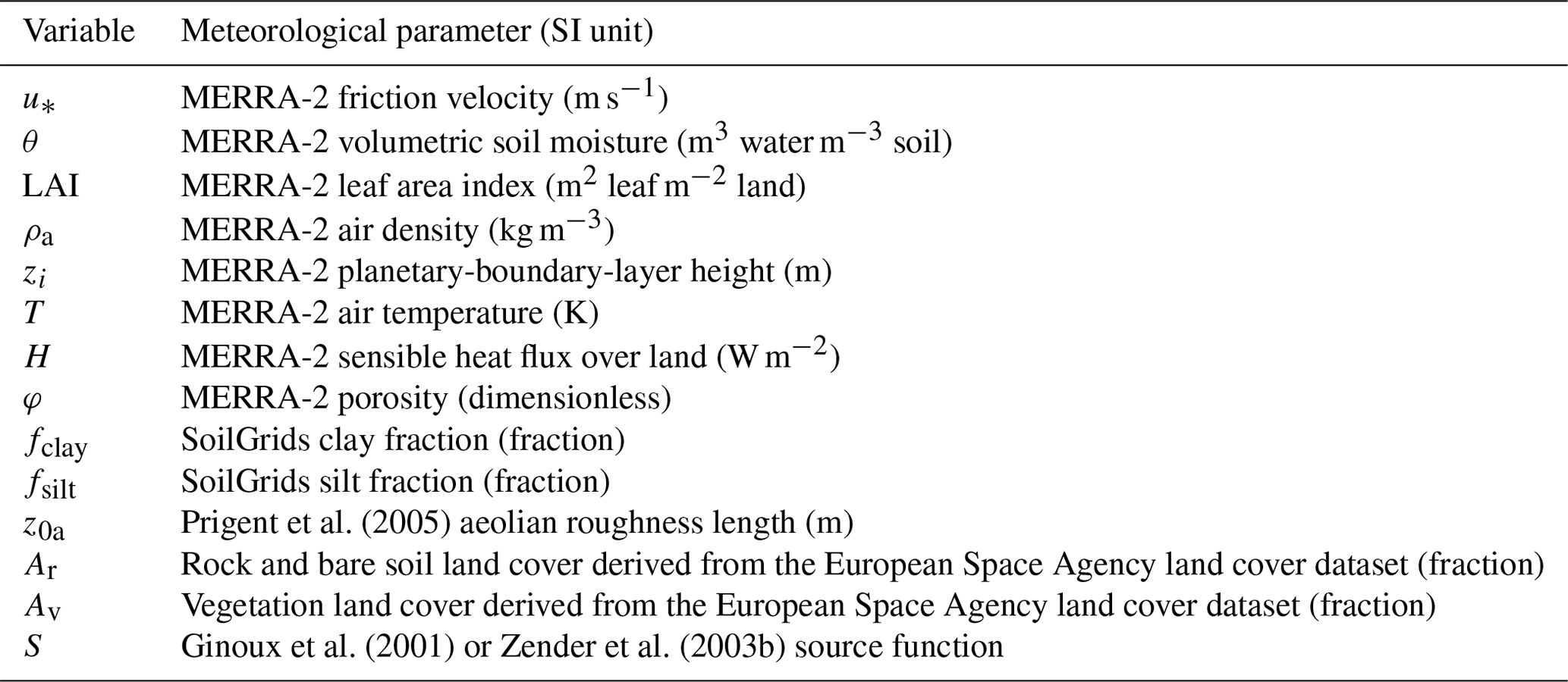
However, many past laboratory studies used the wet sedimentation or wet sieving technique to measure the texture of the soil samples. Wet sieving effectively breaks down soil microaggregates into disaggregated particles and can dissolve soluble minerals (Chatenet et al., 1996), thereby disturbing the estimations of the in situ soil median particle sizes. In contrast, dry sieving causes a minimal disruption to soil microaggregates, and thus Chatenet et al. (1996) argued that the dry-sieved soil PSDs are more representative of the in situ, aggregated soil PSDs. Although the soil texture is a disaggregated soil property, ${\stackrel{\mathrm{‾}}{D}}_{\mathrm{p}}$ might depend on soil texture f_a and other soil properties because the strength of interparticle forces is contingent upon soil texture (the clay and silt content), which governs the extent of soil aggregation. Here, we use measurements from past laboratory studies (see Table S1), which contain site-scale, dry-sieved soil PSDs, wet-sieved soil texture f_a, and other soil properties to investigate their statistical relations and infer a new global distribution of ${\stackrel{\mathrm{‾}}{D}}_{\mathrm{p}}$. All studies listed in Table S1 have dry-sieved soil PSD measurements and the wet-sieved sand, silt, and clay fractions. Many studies have recorded soil organic carbon (SOC; %) and other properties such as calcite (CaCO₃; %), pH value, and bulk density (g cm⁻³). Figure 1a shows the locations of the measurements of the employed soil studies, and the colors show the aridity where the sites are located. Some studies obtained measurements over a relatively large spatial domain, and we plot only one symbol at the domain centroid representing multiple measurements. Many studies reported PSD measurements extending to diameters in excess of 6000 µm, but we used only PSD measurements in the diameter range of 0 and 2000 µm that is relevant to dust emission (Zender et al., 2003a). For each dry-soil PSD measurement, we obtain the aggregated ${\stackrel{\mathrm{‾}}{D}}_{\mathrm{p}}$ by calculating the 50th percentile of the dry-soil PSD.

3.1.2 Deriving a global soil median diameter map

We classify the datasets into arid and nonarid groups, since we are primarily interested in ${\stackrel{\mathrm{‾}}{D}}_{\mathrm{p}}$ over desert regions (although we also display the soil behaviors over nonarid regions). We follow past studies (Mahowald et al., 2006, 2010; Kok et al., 2014b) which defined arid (or dust emission) regions using the criterion of LAI smaller than a threshold LAI_thr, which we take to be 1 (see Sect. 2.3). Section 3.2.2 also describes the MERRA-2 LAI we used in this study to identify the world's arid regions.

After dividing the data into median dry diameters for arid and nonarid soils, we examine the statistical relationships between ${\stackrel{\mathrm{‾}}{D}}_{\mathrm{p}}$ and the soil properties (see Figs. 1b and S2). Figure 1b shows a scatterplot of ${\stackrel{\mathrm{‾}}{D}}_{\mathrm{p}}$ versus the sum of the soil component that produces substantial cohesion, namely the silt and clay fractions ($f_{\mathrm{silt}+\mathrm{clay}}=f_{\mathrm{silt}}+f_{\mathrm{clay}})$. The data exhibit distinctly different trends for nonarid versus arid soils: for nonarid soils, ${\stackrel{\mathrm{‾}}{D}}_{\mathrm{p}}$ increases from 100 µm to greater than 1000 µm with f_silt+clay (regression p value $=\mathrm{7.3}\times {\mathrm{10}}^{-\mathrm{6}})$, likely due to increasing cohesion with increasing clay and silt content. In contrast, ${\stackrel{\mathrm{‾}}{D}}_{\mathrm{p}}$ for arid soils shows a small and statistically insignificant increasing trend with f_silt+clay (p value = 0.77) with a smaller ${\stackrel{\mathrm{‾}}{D}}_{\mathrm{p}}$ variability (50–250 µm). This flat trend indicates that f_silt+clay does not effectively explain the median diameter of aggregated soil particles in arid regions. We examined the relationships of ${\stackrel{\mathrm{‾}}{D}}_{\mathrm{p}}$ with the individual fractions of sand, silt, and clay, as well as with other soil properties including SOC, pH, and CaCO₃ (Fig. S2), but these relationships are not statistically significant. We obtain a surprisingly simple finding from the available measurements that there is limited variability in the aggregated ${\stackrel{\mathrm{‾}}{D}}_{\mathrm{p}}$ over the arid regions across different soil textures. We thus use a constant ${\stackrel{\mathrm{‾}}{D}}_{\mathrm{p}\mathrm{0}}$ as an approximation for arid regions. From Fig. 1b, we summarize the relationship between ${\stackrel{\mathrm{‾}}{D}}_{\mathrm{p}}$ and f_silt+clay as

$$\begin{array}{}\text{(14)}& {\stackrel{\mathrm{‾}}{D}}_{\mathrm{p}}=\left\{\begin{array}{l}{\mathrm{\Psi }}_{\mathrm{0}}+{\mathrm{\Psi }}_{\mathrm{1}}{f}_{\mathrm{silt}+\mathrm{clay}}\\ {\stackrel{\mathrm{‾}}{D}}_{p\mathrm{0}}\end{array}\right.,\begin{array}{l}\text{for}\mathrm{LAI}>{\mathrm{LAI}}_{\mathrm{thr}}\\ \text{for}\mathrm{LAI}\le {\mathrm{LAI}}_{\mathrm{thr}}\end{array},\end{array}$$

where ${\mathrm{\Psi }}_{\mathrm{0}}=\mathrm{7.8}\pm \mathrm{3.7}$ µm, ${\mathrm{\Psi }}_{\mathrm{1}}=\mathrm{124}\pm \mathrm{36}$ µm, ${\stackrel{\mathrm{‾}}{D}}_{\mathrm{p}\mathrm{0}}=\mathrm{127}\pm \mathrm{47}$ µm, and LAI_thr=1 as specified in Eq. (11). This empirical formula suggests that some models' assumptions of the relationship between ${\stackrel{\mathrm{‾}}{D}}_{\mathrm{p}}$ and soil texture were inaccurate (e.g., Table 2 of Laurent et al. (2008) assumed ${\stackrel{\mathrm{‾}}{D}}_{\mathrm{p}}$ decreases with f_silt+clay), and this result could substantially simplify model parameterizations. Additionally, our diameter of 127 µm over arid regions is larger than Z03's assumption of a globally constant optimal diameter of 75 µm. This translates to a modest increase of u_∗ft0 from 0.204 to 0.216 m s⁻¹ (given ρ_a=1.225 kg m⁻³), which slightly decreases global dust emissions by 18 % (see Sect. 4.1). The uncertainty in ${\stackrel{\mathrm{‾}}{D}}_{\mathrm{p}\mathrm{0}}=\mathrm{127}\pm \mathrm{47}$ µm translates to an uncertainty of u_∗ft0 between 0.204 to 0.234 m s⁻¹.

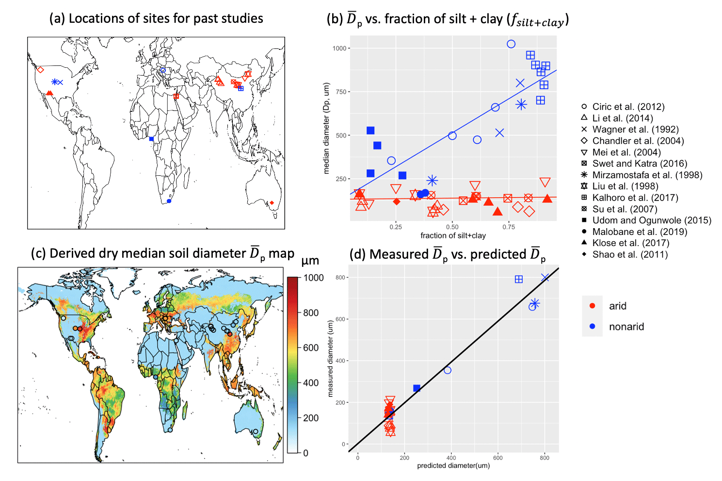
Figure 1 Constructing a global map of the median diameter D_p of aggregated soil particles using soil particle size and texture data. (a) The locations of literature measurements, with symbols indicating the names of the studies and the color indicating the aridity of the locations; a site is classified as arid (red color) if its location has MERRA-2 LAI < 1 and otherwise nonarid (blue color). (b) Literature measurements of soil dry median diameter D_p versus silt + clay fraction (f_silt+clay). (c) The predicted soil median diameter ${\stackrel{\mathrm{‾}}{D}}_{\mathrm{p}}$ map (in µm) derived by projecting our derived ${\stackrel{\mathrm{‾}}{D}}_{\mathrm{p}}$–f_silt+clay relationship of Eq. (14) on the SoilGrids (Hengl et al., 2017) soil texture data (Fig. S3). The circles represent the locations of the sites the same as panel (a), and their colors show the measured median diameter ${\stackrel{\mathrm{‾}}{D}}_{\mathrm{p}}$ at those sites. (d) The predicted ${\stackrel{\mathrm{‾}}{D}}_{\mathrm{p}}$ using Eq. (14) versus measured ${\stackrel{\mathrm{‾}}{D}}_{\mathrm{p}}$ from past studies.

We then project our derived relation between ${\stackrel{\mathrm{‾}}{D}}_{\mathrm{p}}$ and f_silt+clay on the available soil texture and properties database. We employ global soil properties data from the SoilGrids database (Hengl et al., 2014, 2015, 2017), a global soil mapping project that used machine learning (random forest) to regress in situ measurements of soil variables (moisture, temperature, nutrients, etc.). SoilGrids provides global maps of soil texture and other soil properties with a horizontal resolution of 250 m and eight soil depths down to 200 cm (Hengl et al., 2017). We use SoilGrids instead of other available soil databases as it shows better performance against observed soil profiles than other soil databases (Dai et al., 2019). Figure S3 shows the SoilGrids relative fractions of sand, silt, and clay with a 0.1^∘ × 0.1^∘ horizontal resolution for the topmost soil layer. Figure 1c shows our global 0.1^∘ × 0.1^∘ soil median diameter ${\stackrel{\mathrm{‾}}{D}}_{\mathrm{p}}$ map. Following Eq. (14), the arid and semiarid regions are set to have a ${\stackrel{\mathrm{‾}}{D}}_{\mathrm{p}\mathrm{0}}$ of 127 µm, whereas for nonarid regions, ${\stackrel{\mathrm{‾}}{D}}_{\mathrm{p}}$ increases with f_silt+clay. Our derived ${\stackrel{\mathrm{‾}}{D}}_{\mathrm{p}}$ values are largely consistent with the site ${\stackrel{\mathrm{‾}}{D}}_{\mathrm{p}}$ measurements from past studies (overlaid points), showing a similar spatial distribution, with a fit-line slope of 0.98 (p value = 0.007) and an R² of 81 % (Fig. 1d). Note that, since the predictions for arid regions (red points) are a constant without variability, the agreement between the predictions and observations is essentially dominated by the linear ${\stackrel{\mathrm{‾}}{D}}_{\mathrm{p}}$–f_silt+clay relation over nonarid regions (blue points). Figure 1d shows that Eq. (14) gives satisfactory agreement in predicting global ${\stackrel{\mathrm{‾}}{D}}_{\mathrm{p}}$, but dust emission modeling will depend exclusively on the predicted ${\stackrel{\mathrm{‾}}{D}}_{\mathrm{p}}$ over arid regions. We anticipate that as more measurements emerge in the future, more statistical or machine learning modeling approaches can more robustly decipher the intricate relationships between ${\stackrel{\mathrm{‾}}{D}}_{\mathrm{p}}$ and various soil properties over arid regions.

Since nonarid regions of LAI > 1 will generate zero emissions (Eq. 11), we simplify Eq. (14) and Fig. 1c by imposing a globally constant ${\stackrel{\mathrm{‾}}{D}}_{\mathrm{p}\mathrm{0}}=\mathrm{127}$ µm.

3.2 A wind drag partition scheme for decreasing wind stress and erosion

We now present a methodology to account for the wind drag partition effect due to nonerodible roughness elements including vegetation and rocks that protect the bare soil by absorbing part of the surface wind stress. We calculate the rock drag partition f_eff,r using z_0a since global z_0a observations are available, and we calculate the vegetation drag partition f_eff,v using vegetation cover which is a proxy of λ (e.g., Shao et al., 1996; Okin, 2008), since gridded plant cover is often parameterized in GCMs (e.g., Wu et al., 2016; Foroutan et al., 2017; Meier et al., 2022). Here we use two separate drag partition schemes (Marticorena and Bergametti, 1995; Okin, 2008) to quantify the roughness effect of rocks (Sect. 3.2.1) and vegetation (Sect. 3.2.2), respectively. Then, we propose a unifying approach to combine the two effects into a hybrid factor F_eff (Sect. 3.2.3).

3.2.1 Drag partition due to roughness of rocks

In this study, we use the aeolian roughness length z_0a to quantify the drag partition effect due to rocks. Whereas the smooth z_0s and the aerodynamic momentum z_0m can be derived from pre-existing datasets, it is more challenging to quantify the aeolian z_0a. Existing efforts employed satellite and field measurements to quantify the roughness over deserts (e.g., Greeley et al., 1997; Roujean et al., 1997; Marticorena et al., 2004; Laurent et al., 2005; Prigent et al., 2005; Marticorena et al., 2006; Prigent et al., 2012). For instance, Marticorena et al. (1997) and Callot et al. (2000) developed a 1^∘ × 1^∘ z_0a map over Africa and the Middle East by combining topographic data, geological information, aerial pictures, and in situ observations. Prigent et al. (2005) and Prigent et al. (2012) further used radar measurements to yield global maps of backscatter coefficient, which is a measure of surface roughness because rougher surfaces generally scatter more radar signals to different directions and reduce the backscattering. Comparisons between satellite backscattering signals and field measurements of z_0a yielded an empirical formula for extrapolating a global dataset of backscattering signal to global z_0a. We use here the global aeolian z_0a dataset from Prigent et al. (2005) (hereafter Pr05), which contains the climatological monthly mean z_0a (12 monthly values per grid) derived from the backscatter coefficient observed by the scatterometer at 5.3 GHz on board the European Remote Sensing (ERS) satellite. Since satellite z_0a measurements could quantify the roughness of both rocks and vegetation, we take the minimum value out of the 12 months for all grids to obtain a static aeolian z_0a map to eliminate as much as possible the vegetation effect on the inferred roughness. Furthermore, we apply this map over arid regions only (LAI < 1), where the backscatter signal is mostly generated by rocks with little contribution from vegetation roughness. The resulting 2-D map of z_0a (in centimeters) thus mostly represents time-invariant rock roughness and is plotted in Fig. 2a.

Marticorena and Bergametti (1995) derived a parameterization to quantify the drag partition effect using both z_0a and z_0s. They assumed that this equation is valid for roughness elements that are not too closely spaced (small wake), i.e., z_0a<1 cm (Darmenova et al., 2009). Here we use their semiempirical equation to quantify the drag partition due to rocks, f_eff,r (also see Eq. 8):

$$\begin{array}{}\text{(15)}& f_{\mathrm{eff},\mathrm{r}}=\mathrm{1}-{\displaystyle \frac{\ln \left(\frac{z_{\mathrm{0}\mathrm{a}}}{z_{\mathrm{0}\mathrm{s}}}\right)}{\ln \left[b_{\mathrm{1}}{\left(\frac{X}{z_{\mathrm{0}\mathrm{s}}}\right)}^{b_{\mathrm{2}}}\right]}},\end{array}$$

where X is the distance downstream the point of discontinuity in roughness, a length parameter that scales with the IBL height δ behind the obstacle in Eq. (8), i.e., $\frac{\mathit{\delta }}{z_{\mathrm{0}\mathrm{s}}}=b_{\mathrm{1}}{\left(\frac{X}{z_{\mathrm{0}\mathrm{s}}}\right)}^{b_{\mathrm{2}}}$ following Marticorena and Bergametti (1995), and b₁=0.7 and b₂=0.8 are empirical constants (King et al., 2005; Darmenova et al., 2009). X should be a function of land type and implicitly space and time, but thus far most dust modeling studies have used a global constant for X (e.g., Darmenova et al. (2009) used a globally constant X=0.1 m). We use a globally constant X=10 m in this study, which is different from what the past studies suggested, because the scale of the rocks and plants we focus on in deserts is larger and is of the order of 10⁰–10¹ m. Some studies considered even larger roughness and used X∼122 m for vegetated deserts (MacKinnon et al., 2004). We then obtain z_0s from our derived global dataset of ${\stackrel{\mathrm{‾}}{D}}_{\mathrm{p}}$ in Sect. 3.1 using Eq. (7). When nonerodible roughness elements are abundant over a surface, z_0a≫z_0s and $f_{\mathrm{eff},\mathrm{r}}\ll \mathrm{1}$, causing the sheltering of the bare soil from the wind; when there are few roughness elements, z_0a is small and close to z_0s, and thus f_eff,r approaches 1. In Fig. 2a, the red areas with very small z_0a are the most susceptible regions for dust emission. Figure 2a also shows that most arid and semiarid regions have z_0a<0.2 cm, such that Eq. (15) can follow the criterion (z_0a<1 cm) in Darmenova et al. (2009) well. Figure 2b shows the global f_eff,r over arid regions, which is dominated by the spatial pattern of z_0a in Fig. 2a given f_eff,r is governed purely by z_0a.

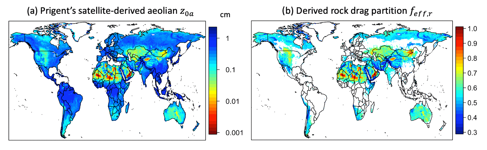
Figure 2 Global roughness length and rock drag partition factor maps at a horizontal resolution of 0.25^∘ × 0.25^∘. (a) Global mesoscale aeolian roughness length z_0a (in centimeters) derived by Prigent et al. (2005). (b) Global static rock drag partition factor f_eff,r derived by Eq. (15) following Marticorena and Bergametti (1995), derived over arid and semiarid regions defined as MERRA-2 LAI < 1 in this study. The color schemes are set such that the most erodible regions appear red.

3.2.2 Drag partition due to roughness of vegetation

Unlike the very static and slowly evolving rock roughness, vegetation changes temporally. To include the effect of these dynamic vegetation changes on the drag partition, we follow the approach of Okin (2008) (hereafter O08), which uses unvegetated gap size (the distance between neighboring plants) to characterize the variability of the reduced wind stress. O08 argued that his scheme represents an advancement over the classical R93 scheme, since R93 uses the roughness density (or lateral cover) λ, which only quantifies how much roughness is on a surface but not how that roughness is spatially distributed. O08 pointed out that, given the same λ, roughness elements divided into small blocks spread over the soil surface would be more effective than elements stacked up like a telephone pole in partitioning wind stress (see Fig. 3 in Okin, 2008). Okin argued that since Raupach's model neglects the spatial variability of λ, the resulting simulated emission flux using the R93 scheme in Okin's paper decreased rapidly with increasing λ and unrealistically reached zero at relatively low λ. To partially compensate for this error, R93 introduced a tuning parameter m (Eq. 9a), serving to reduce the effective λ and thereby reducing the rapid decrease in dust flux. However, m is a tuning parameter not derived from first principles, and it is not clear how m changes over different surface conditions. Therefore, we use the O08 model here to better characterize the spatial variability of wind stress and the resulting dust emissions.

Here we describe the O08 scheme and adapt it for use in LSMs and GCMs. O08 assumes u_∗ drops significantly when encountering a roughness element (plant) and gradually recovers at the lee (downwind region) of the plant as a function of distance x, following

$$\begin{array}{}\text{(16a)}& u_{\ast \mathrm{s}}(x/h)=u_{\ast }\left[f_{\mathrm{0}}+(\mathrm{1}-f_{\mathrm{0}})\left(\mathrm{1}-e^{-\frac{x/h}{c}}\right)\right],\end{array}$$

where $x/h$ is the dimensionless downwind distance from an obstacle normalized by vegetation height h (m), $f_{\mathrm{0}}=\frac{u_{\ast \mathrm{s}}}{u_{\ast }}{|}_{x=\mathrm{0}}$ is the friction velocity ratio immediately behind the obstacle, and c is the dimensionless e-folding distance (normalized by h) over which u_∗s locally recovers to u_∗. In this formulation, the local drag partition factor due to vegetation as a function of distance x is

$$\begin{array}{}\text{(16b)}& f_{\mathrm{local}}\left({\displaystyle \frac{x}{h}}\right)={\displaystyle \frac{u_{\ast \mathrm{s}}}{u_{\ast }}}=f_{\mathrm{0}}+(\mathrm{1}-f_{\mathrm{0}})(\mathrm{1}-e^{-\frac{x/h}{c}}).\end{array}$$

Note that in the limit of $x/h\to \mathrm{\infty }$,$u_{\ast \mathrm{s}}\to u_{\ast }$. O08 used measurements from Bradley and Mulhearn (1983) and fitted f₀=0.32 and c=4.8 (i.e., the e-folding distance of u_∗s recovery to u_∗ is 4.8 times the plant height h) for semiarid regions.

In order to use Eq. (16b) to obtain the drag partition f_eff,v relevant to a regionally vegetated area that is more applicable to GCMs, one needs to calculate an integral for the averaged and aggregated effect of drag partitioning f_eff,v (see Eq. 20a) instead of a locally varying f_local (Eq. 16b). Therefore, Okin employed a probability distribution function as a function of distance $x/h$ to indicate the importance (or weight) of f_local at any $x/h$ to the averaging of f_eff,v (McGlynn and Okin, 2006; Okin, 2008). The PDF is an exponential decay such that the weight of f_local decreases with distance $x/h$, so f_local at the immediate lee of the obstacle (which is smaller and close to f₀) has more weight than the f_local farther away (which is larger and tends to 1). From McGlynn and Okin (2006), the PDF is a function of normalized distance $x/h$:

$$\begin{array}{}\text{(17a)}& {\displaystyle }{P}_{\mathrm{d}}(x/h)={\displaystyle \frac{\mathrm{1}}{K}}{e}^{-\frac{x/h}{K}}\text{(17b)}& {\displaystyle }K\equiv L/h,\end{array}$$

where L (m) is the mean gap length between obstacles (plants), which is conceptually related to f_v; and K is the normalized gap length, which is the gap length L scaled by the plant height h. Physically, P_d is the probability that there is not another obstacle present within a downwind distance $x/h$. This exponential decay implies that the farther away from a plant (larger $x/h)$, the higher the likelihood that there is another plant present within the downwind distance $x/h$, with the normalized gap length K quantifying the e-folding distance of the probability. This PDF governs the spatial domain over which u_∗s recovers.

For O08, the mean gap length between obstacles K is the only required input for calculating the drag partition, since f₀ and c are assumed to be invariant to surface conditions and desert biome. K can be expressed as a function of f_v using some simple assumptions. First, O08 argued that the vegetation cover fraction is simply $f_v\equiv \frac{W}{L+W}$, where L is the mean gap length and W is the mean width of the plants within that vegetated area. Rearranging gives

$$\begin{array}{}\text{(18a)}& L=W({\displaystyle \frac{\mathrm{1}}{f_{\mathrm{v}}}}-\mathrm{1}).\end{array}$$

Then we assume plants in arid regions (e.g., shrubs) are approximately hemispheres with radius R. Then, the plant height h=R and width W=2R are related by W=2h, which can be substituted into Eq. (18a) to yield

$$\begin{array}{}\text{(18b)}& K\equiv {\displaystyle \frac{L}{h}}=\mathrm{2}\left({\displaystyle \frac{\mathrm{1}}{f_{\mathrm{v}}}}-\mathrm{1}\right),\end{array}$$

and thus we related K to f_v. f_v could be measured at the local level, and thus O08 was frequently applied in field studies (e.g., Li et al., 2013; Pierre et al., 2014a). However, what is novel in our study is that we are the first to propose the implementation of O08 into LSMs, because Eq. (18b) shows us that O08 could be formulated as a function of f_v, which is a grid-level parameter. Here we propose to follow the Mahowald et al. (2006) assumption in Eq. (11) and approximate vegetation cover fraction as $f_{\mathrm{v}}=\mathrm{1}-f_{\mathrm{bare}}=\mathrm{LAI}/{\mathrm{LAI}}_{\mathrm{thr}}$. Equation (18b) becomes

$$\begin{array}{}\text{(18c)}& K\equiv {\displaystyle \frac{L}{h}}=\mathrm{2}\left({\displaystyle \frac{\mathrm{1}}{f_{\mathrm{v}}}}-\mathrm{1}\right)=\mathrm{2}({\displaystyle \frac{\mathrm{1}}{\mathrm{LAI}/{\mathrm{LAI}}_{\mathrm{thr}}}}-\mathrm{1}),\end{array}$$

where we assume LAI_thr=1 (in Eq. 11). The assumption of f_v∼LAI is valid if we reasonably assume that leaf areas over arid regions overlap relatively little with each other. We note that by using LAI to quantify f_v in Eq. (18c), we are only accounting for the vegetation drag partitioning due to green (photosynthetic) vegetation and miss that due to brown (nonphotosynthetic) vegetation. In the future, it is warranted that Eq. (18b) includes other proxies of brown vegetation drag partitioning, such as the vegetation cover quantified by Guerschman et al. (2015), which was adopted by later dust modeling studies such as Klose et al. (2021) and Huang and Foroutan (2022).

To estimate the reduced emission flux, O08 uses an integration approach without quantifying f_eff,v. O08 calculates the reduced dust emission flux F_red (kg m⁻² s⁻¹) by locally integrating the emission F_d following the spatially varying u_∗s over the normalized distance $x/h$:

$$\begin{array}{}\text{(19)}& F_{\mathrm{red}}=\underset{x/h=\mathrm{0}}{\overset{\mathrm{\infty }}{\int }}{P}_{\mathrm{d}}\left({\displaystyle \frac{x}{h}}\right)F_{\mathrm{d}}\left[u_{\ast \mathrm{s}}\left({\displaystyle \frac{x}{h}}\right)\right]d\left({\displaystyle \frac{x}{h}}\right),\end{array}$$

where F_d (kg m⁻² s⁻¹) is the local emission as a function of u_∗s which is itself a function of $x/h$. In the integration, F_d needs to be weighted by P_d (which means F_d at large $x/h$ has proportionally less importance) because as $x/h$ increases, the likelihood of the presence of another obstacle gets larger and larger, which will hinder the recovery of u_∗s to u_∗. Integrating the emission flux F_d from zero to infinity gives a reduced emission flux F_red, which will be smaller than the emission flux without roughness elements, defined as $F_{\mathrm{bare}}={\int }_{x/h=\mathrm{0}}^{\mathrm{\infty }}{P}_{\mathrm{d}}\left(\frac{x}{h}\right)F_{\mathrm{d}}\left(u_{\ast }\right)d\left(\frac{x}{h}\right)=F_{\mathrm{d}}\left(u_{\ast }\right)$, in which F_d is a constant in space since $u_{\ast \mathrm{s}}=u_{\ast }$ is a constant without obstacles.

However, since we need to also combine the vegetation drag partition with the rock partition effects, we need to quantify f_eff,v in order to form a hybrid drag partition factor for LSMs. Instead of directly implementing Eq. (19a) into LSMs, we require an alternative approach of quantifying f_eff,v such that $F_{\mathrm{d}}\left(f_{\mathrm{eff},\mathrm{v}}{u}_{\ast }\right)=F_{\mathrm{red}}$. Quantifying f_eff,v for O08 can be useful for comparisons against f_eff,v from other schemes such as R93 and Klose et al. (2021). In addition, quantifying f_eff,v for O08 makes it possible to generate a high-resolution, diagnostic f_eff,v dataset for mechanistic models with different resolutions as a model input.

An approach of evaluating f_eff,v from O08 was proposed by Pierre et al. (2014a). They obtained the expected value of the shear stress ratio $u_{\ast \mathrm{s}}/u_{\ast }$ (SSR in Okin, 2008) between obstacles by evaluating the integral of $u_{\ast \mathrm{s}}/u_{\ast }$ weighted by P_d, which represents the averaged f_local (in Eq. 16b) across the vegetated area and perfectly fits our purposes for implementing f_eff,v into LSMs:

$$\begin{array}{}\text{(20a)}& \begin{array}{rl}{f}_{\mathrm{eff},\mathrm{v}}& =\underset{x/h=\mathrm{0}}{\overset{\mathrm{\infty }}{\int }}{P}_{\mathrm{d}}\left({\displaystyle \frac{x}{h}}\right)\left[{\displaystyle \frac{u_{\ast \mathrm{s}}\left(\frac{x}{h}\right)}{u_{\ast }}}\right]d\left({\displaystyle \frac{x}{h}}\right)\\ & =\underset{x/h=\mathrm{0}}{\overset{\mathrm{\infty }}{\int }}{P}_{\mathrm{d}}\left({\displaystyle \frac{x}{h}}\right)f_{\mathrm{local}}\left({\displaystyle \frac{x}{h}}\right)d\left({\displaystyle \frac{x}{h}}\right)\end{array}.\end{array}$$

Substituting Eq. (17) for P_d into Eq. (20a) and analytically evaluating the integral gives a simple algebraic equation for f_eff,v (Pierre et al., 2014a), representing the aggregated vegetation drag partition effect at the grid level:

$$\begin{array}{}\text{(20b)}& f_{\mathrm{eff},\mathrm{v}}={\displaystyle \frac{K+f_{\mathrm{0}}c}{K+c}}.\end{array}$$

This elegant formula conveys a clear physical intuition: if the obstacle does not effectively dissipate momentum (f₀→1), $f_{\mathrm{eff},\mathrm{v}}\to \mathrm{1}$; if land is densely covered by vegetation (gap length K→0), $f_{\mathrm{eff},\mathrm{v}}\to f_{\mathrm{0}}(=\mathrm{0.32})$, the shear stress ratio at the immediate lee of the obstacle. An advantage of this approach is that it can be easily adopted by gridded models since modelers only need to code an algebraic equation instead of an integral.

We calculate 0.5^∘ × 0.625^∘ global hourly f_eff,v data for Okin's model, using Eqs. (18c) and (20b) with hourly MERRA-2 LAI. We note that MERRA-2 LAI is based on the Advanced Very High Resolution Radiometer (AVHRR) observations (Reichle et al., 2017). Figure 3a shows the annually averaged MERRA-2 LAI for the year 2006 over arid regions with LAI < 1 (seasonal LAI maps are also shown in Fig. S4), and Fig. 3b shows the corresponding mean f_eff,v for areas where LAI < 1. The LAI plot shows the most erodible regions on Earth.

Figure 3 Vegetation drag partition factor f_eff,v derived from the Okin (2008) and Pierre et al. (2014) drag partition model for the year 2006 on a 0.5^∘ × 0.625^∘ grid. (a) Annual mean MERRA-2 LAI, with color bar saturated at a value of 1. (b) Annually averaged f_eff,v derived using the Okin (2008) and Pierre et al. (2014) drag partition model. White areas indicate water body, ice/snow, or LAI > 1.

3.2.3 Combining drag partition factors of rocks and vegetation

After obtaining both the static f_eff,r map of rocks and the time-varying f_eff,v map of vegetation, we now propose a methodology to combine the two drag partition sources to capture and represent the total drag partition effect for dust emission. LSMs need a single drag partition factor capturing all roughness effects to estimate the total reduction of the surface winds. Thus, we compute a hybrid drag partition factor map F_eff that can be used as input for dust modules in GCMs. To achieve this, we need to know the fractions of a grid that consists of areas dominated by rocks and areas dominated by plants, which can be obtained from several recent studies (Lawrence et al., 2016; ESA, 2017; Klein Goldewijk et al., 2017; Kobayashi et al., 2017). We obtained these data from the European Space Agency Climate Change Initiative (ESA CCI) dataset (https://www.esa-landcover-cci.org/?q=node/164, last access: 21 June 2022). The land cover product classifies the land cover of the whole globe into 37 categories (Li et al., 2018), with relevant land cover over arid regions such as shrub, herbaceous, sparse vegetation, cropland, grassland, and consolidated (gravels and rocks) and unconsolidated (soil) bare land. This dataset has a horizontal resolution of 300 m, making the dataset capable of counting the portion of the grid consisting of rocks and vegetation over a larger MERRA-2 0.5^∘ × 0.625^∘ grid box (a MERRA-2 grid box consists of ∼ 35 000 grids of 300 m). This dataset gives a representation of the annually varying land covers, so the rock and vegetation area fractions we use are a function of space only within the simulation year of 2006. We describe our approach to synthesizing the ESA CCI land cover maps and drag partition datasets in the following.

We incorporate the drag partition effects by identifying two roughness regimes using the ESA CCI dataset. The first regime is the rock regime (Fig. 4a), for which we combine the consolidated (gravel and rocks) and unconsolidated (soil) bare land types (types 34–36). This regime is subject to the rock drag partition effect. The second regime is the vegetation regime (Fig. 4b), which includes different vegetation types such as shrubland and herbaceous (types 19–23, 28–29, 32), sparse vegetation (types 26–27), cropland (types 2–5), grassland (type 24), mixed vegetation (type 18), and other vegetation mosaic (types 6–7). Since O08 does not specify the differences in drag partition for different plant functional types (PFTs), here we assume all PFTs produce the same drag partition effect. The overall drag partition effect F_eff for a grid is thus defined by the summation of emissions, with emission F_d,r over the rock regime with a fractional area of A_r, and emission F_d,v over the vegetation regime with another fractional area A_v:

$$\begin{array}{}\text{(21a)}& \begin{array}{rl}{F}_{\mathrm{d}}\left(u_{\ast }{F}_{\mathrm{eff}}\right)& =A_{\mathrm{r}}{F}_{\mathrm{d},\mathrm{r}}+A_{\mathrm{v}}{F}_{\mathrm{d},\mathrm{v}}=A_{\mathrm{r}}{F}_{\mathrm{d}}\left(u_{\ast }{f}_{\mathrm{eff},\mathrm{r}}\right)\\ & +A_{\mathrm{v}}{F}_{\mathrm{d}}\left(u_{\ast }{f}_{\mathrm{eff},\mathrm{v}}\right)\end{array}.\end{array}$$

Given that dust emissions approximately scale with the cube of u_∗s (Zender et al., 2003a; Kok et al., 2014b) and neglecting the effect of the dust emission threshold, Eq. (21a) can be simplified to

$$\begin{array}{}\text{(21b)}& F_{\mathrm{eff}}^{\mathrm{3}}=A_{\mathrm{r}}{f}_{\mathrm{eff},\mathrm{r}}^{\mathrm{3}}+A_{\mathrm{v}}{f}_{\mathrm{eff},\mathrm{v}}^{\mathrm{3}},\end{array}$$

such that F_eff is simply the weighted mean of drag partition effects. The fractional areas are simply calculated by counting the total occupied area of the ESA CCI land cover corresponding to a certain regime and then dividing by the total area of the grid box. We use Eq. (21b) to obtain the spatiotemporally varying $F_{\mathrm{eff}}(\mathrm{long},\mathrm{lat},t)$, given $f_{\mathrm{eff},\mathrm{v}}(\mathrm{long},\mathrm{lat},t)$ and A_r, A_v, and f_eff,r as functions of (long,lat). We then apply the obtained F_eff here to Eq. (6) to yield u_∗s for the dust emission equation. We discuss in Sects. 5 and S6.2 the caveats and limitations of this hybrid drag partition scheme.

Figure 4a–b show the fractional areas of the two regimes. The rock regime (Fig. 4a) is located mostly over the Sahara, the Middle East, and the Asian deserts. The vegetation regime (Fig. 4b) is concentrated mostly over Australia, the United States, South America, and southern Africa. Figure 4c shows the resulting annually averaged F_eff using Eq. (21b). The regions with the highest F_eff are the Bodélé Depression, El Djouf, the Arabian Desert, and Taklamakan due to high f_eff,r. The Strzelecki–Sturt Stony deserts in Australia, the Kyzylkum, and Patagonia also have high F_eff (∼ 0.7) due to high f_eff,v. Regions with both high rock and vegetation roughness are located in parts of the Middle East and North America with low F_eff values.

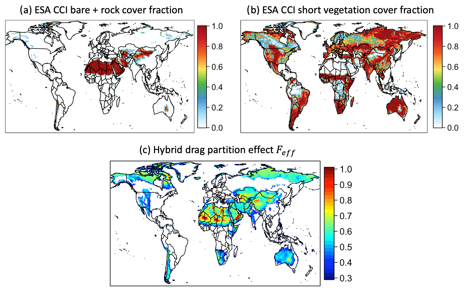
Figure 4 The 0.5^∘ × 0.625^∘ hybrid drag partition factor F_eff incorporated using the European Space Agency Climate Change Initiative (ESA CCI) dataset. (a–b) The fractional areas of (a) the rock regime (consolidated/unconsolidated land) and (b) the vegetation regime (shrubs, herbaceous plants, croplands, grassland, and sparse vegetation) over arid regions. (c) The hybrid drag partition factor F_eff by a combination of rock drag partition f_eff,r and vegetation drag partition f_eff,v for the year 2006.

3.3 Parameterizing the dust emission intermittency

The above improvements enable a more accurate calculation of emission when wind speeds are sufficient to initiate dust emission. Next, we will improve the calculation of the resulting dust emission flux by accounting for the effects of boundary-layer turbulence on dust emission intermittency. Dust emission intermittency exists because saltation is driven by turbulent surface winds, which exhibit strong spatiotemporal fluctuations in speed and direction. Instantaneous winds can thus pass within short timescales across the emission thresholds for initiating or ceasing saltation (Martin and Kok, 2018). Consequently, saltation can be highly intermittent (Comola et al., 2019b), with pronounced variability on timescales of seconds to hours (Dupont et al., 2013). In contrast, existing dust emission parameterizations describe saltation as uniform in time and space and driven by a constant downward momentum flux within a model time step. The disconnect between the reality of intermittent dust emissions and uniform emissions in current theories is likely contributing to the poor performance of dust emission simulations (Barchyn et al., 2014; Todd et al., 2008). Comola et al. (2019b) argued that the intermittency effect is more prevalent for regions with low-intensity dust emissions when u_∗s is regularly fluctuating around the threshold to turn on or shut off dust emissions. Neglecting intermittent dust emissions in current models thus likely degrades the accuracy of dust emission simulations for arid regions during low-wind periods and for marginal dust source regions such as semiarid areas (since soil cohesion increases u_∗ft but does not affect u_∗it), which dominate in much of the Southern Hemisphere (Ginoux et al., 2012; Ito and Kok, 2017).

Accounting for the intermittency effect on dust emission fluxes is complicated by the hysteresis of dust emission due to the existence of double thresholds for dust emission physics. The instantaneous wind at the saltation level ${\stackrel{\mathrm{̃}}{u}}_{\mathrm{s}}$ (we use the tilde to denote instantaneous quantities and take away the asterisk to denote winds at the saltation level of z_sal∼0.1 m using Eq. (S4a) instead of a velocity scale) needs to exceed the fluid threshold u_ft (also defined at the saltation level) to initiate saltation, but it only needs to exceed a smaller impact threshold u_it to sustain it (Kok et al., 2012; Martin and Kok, 2018; Comola et al., 2019b). When ${\stackrel{\mathrm{̃}}{u}}_{\mathrm{s}}$ at a moment lies between both thresholds $(u_{\mathrm{it}}<{\stackrel{\mathrm{̃}}{u}}_{\mathrm{s}}<u_{\mathrm{ft}})$, saltation is active if transport was more recently initiated $({\stackrel{\mathrm{̃}}{u}}_{\mathrm{s}}>u_{\mathrm{ft}})$ and inactive if transport was more recently terminated $({\stackrel{\mathrm{̃}}{u}}_{\mathrm{s}}<u_{\mathrm{it}})$. This process is known as hysteresis (Kok, 2010; Martin and Kok, 2018; Comola et al., 2019b). As a result, if u_s (mean of ${\stackrel{\mathrm{̃}}{u}}_{\mathrm{s}}$ within a model time step) is between u_it and u_ft, there will be fluctuating emission fluxes in reality, while models using a fluid threshold scheme would predict zero emission within a model time step, thereby underestimating the emissions. Meanwhile, models using an impact threshold scheme without considering turbulence will have uniform positive dust emission within the time interval. However, because in reality high-frequency winds can pass below u_it and shut off dust emissions, using average u_s in an impact threshold scheme will overestimate dust emissions. It is thus important for GCMs to account for the effects of turbulence causing both intermittency and hysteresis of dust emission.

As GCMs have a relatively large time step and a coarse horizontal resolution (e.g., ∼ 30 min for a 1^∘ GCM), they are not designed to resolve turbulence and cannot capture high-frequency (∼ 0.1–5 min) turbulent wind speed fluctuations. As a result, models cannot directly simulate the dust emission intermittency. Therefore, accounting for intermittent dust emission requires a parameterization that links the low-frequency (∼ 30 min) variables of boundary-layer turbulence that are resolved in GCMs to the high-frequency intermittency dynamics. Comola et al. (2019b) formulated a parameterization (hereafter the C19 scheme) of intermittent saltation fluxes by quantifying wind fluctuations due to both shear-driven and buoyancy-driven turbulence in terms of resolved model parameters, including u_it and the Monin–Obukhov length L. C19 showed that when a dust emission equation employs u_it and accounts for the intermittency effect, it can successfully capture the magnitudes of small dust fluxes otherwise missed by models using u_ft (Fig. 3 of Comola et al., 2019b). The C19 scheme will thus moderate the temporal variability of modeled dust emissions due to diurnal wind cycles continuously crossing the thresholds. Additionally, it will also capture more lower-intensity emissions over marginal sources missed by many current models (Zhao et al., 2022).

In the C19 scheme, the dust emission flux F_d is calculated using u_∗it instead of u_∗ft. We update K14 (Eq. 13) with $u_{\ast \mathrm{t}}=u_{\ast \mathrm{it}}$ as the threshold, giving

22a$$\begin{array}{}\text{(22a)}& {\displaystyle }\begin{array}{rl}{F}_{\mathrm{d}}& =C_{\mathrm{tune}}{C}_{\mathrm{d}}{f}_{\mathrm{bare}}{f}_{\mathrm{clay}}{\displaystyle \frac{{\mathit{\rho }}_{\mathrm{a}}\left(u_{\ast \mathrm{s}}^{\mathrm{2}}-u_{\ast \mathrm{it}}^{\mathrm{2}}\right)}{u_{\ast \mathrm{it}}}}{\left({\displaystyle \frac{u_{\ast \mathrm{s}}}{u_{\ast \mathrm{it}}}}\right)}^{\mathit{\kappa }}\\ & \text{for}{u}_{\ast \mathrm{s}}>u_{\ast \mathrm{it}},\end{array}\end{array}$$

where C_d is still a function of u_∗st, and $u_{\ast \mathrm{st}}=u_{\ast \mathrm{ft}}\sqrt{{\mathit{\rho }}_{\mathrm{a}}/{\mathit{\rho }}_{\mathrm{a}\mathrm{0}}}$ is the same standardized fluid threshold as in the default K14, and u_∗it is computed using Eq. (5). Because u_∗it <u_∗ft, this modified equation allows more small dust fluxes over the marginal source regions that are otherwise missed by employing u_∗ft as the threshold (see Figs. 7g–h).

Next, we account for the intermittency effect by introducing the intermittency factor η, which is the fraction of time that saltation is active in a model time step (e.g., ∼ 30 min). η corrects the horizontal sand saltation flux, which scales with dust emission flux (Shao et al., 1993), thereby also representing the fraction of time that dust emission is active in a model time step. C19 accounts for the effect of intermittency by multiplying dust emission by η as follows:

$$\begin{array}{}\text{(22b)}& F_{\mathrm{d},\mathit{\eta }}=\mathit{\eta }{F}_{\mathrm{d}},\end{array}$$

where $\mathit{\eta }\in [\mathrm{0},\mathrm{1}]$. Note that C19 parameterizes η using wind information at the typical saltation height of z_sal=0.1 m instead of the velocity scales. η is thus formulated as a function of the wind speeds u_s, u_it, and u_ft at height z_sal (see Sect. S3 Eqs. S3–S6) and the standard deviation ${\mathit{\sigma }}_{{\stackrel{\mathrm{̃}}{u}}_{\mathrm{s}}}$ of the instantaneous ${\stackrel{\mathrm{̃}}{u}}_{\mathrm{s}}$ (Eq. 23):

$$\begin{array}{}\text{(22c)}& \mathit{\eta }=\mathit{\eta }(u_{\mathrm{s}},{\mathit{\sigma }}_{{\stackrel{\mathrm{̃}}{u}}_{\mathrm{s}}},u_{\mathrm{it}},u_{\mathrm{ft}}).\end{array}$$

${\mathit{\sigma }}_{{\stackrel{\mathrm{̃}}{u}}_{\mathrm{s}}}$ is defined given that ${\stackrel{\mathrm{̃}}{u}}_{\mathrm{s}}$ can be described by a normal distribution (Chu et al., 1996), with its mean being the model time step mean (at 0.1 m) u_s and its standard deviation ${\mathit{\sigma }}_{{\stackrel{\mathrm{̃}}{u}}_{\mathrm{s}}}$. From Eq. (22c), η→1 when u_s≫u_ft (active emission for the whole time step) and η→0 when u_s≪u_it (no emission for the time step). The further away u_s is from the thresholds u_ft and u_it, the smaller the probability of the instantaneous ${\stackrel{\mathrm{̃}}{u}}_{\mathrm{s}}$ sweeping across the thresholds and the more dichotomous η behaves (either zero or 1). If u_s is very close to u_ft or u_it, or is indeed between them $(u_{\mathrm{it}}<{\stackrel{\mathrm{̃}}{u}}_{\mathrm{s}}<u_{\mathrm{ft}})$, the frequency of crossing the threshold is determined by the magnitude of the turbulent fluctuation ${\mathit{\sigma }}_{{\stackrel{\mathrm{̃}}{u}}_{\mathrm{s}}}$. ${\mathit{\sigma }}_{{\stackrel{\mathrm{̃}}{u}}_{\mathrm{s}}}$ is parameterized using the similarity theory (Panofsky et al., 1977):

$$\begin{array}{}\text{(23)}& {\mathit{\sigma }}_{{\stackrel{\mathrm{̃}}{u}}_{\mathrm{s}}}=u_{\ast \mathrm{s}}{\left(\mathrm{12}-\mathrm{0.5}{\displaystyle \frac{z_{\mathrm{i}}}{L}}\right)}^{\mathrm{1}/\mathrm{3}}\text{for}\mathrm{12}-\mathrm{0.5}{\displaystyle \frac{z_{\mathrm{i}}}{L}}\ge \mathrm{0},\end{array}$$

where L is the Obukhov length, and z_i is the modeled PBL height. Note that MERRA-2 does not provide L output, and in this study we computed L from the MERRA-2 outputs of u_∗, ρ_a, sensible heat flux H, and temperature T for our simulations (see Sect. S3). In boundary-layer dynamics, turbulence is generated by mechanical shear and buoyancy (Stull, 1988). From Eq. (23), high-frequency wind fluctuations ${\mathit{\sigma }}_{{\stackrel{\mathrm{̃}}{u}}_{\mathrm{s}}}$ increase with shear ($u_{\ast \mathrm{s}}>\mathrm{0})$ and buoyancy (L<0). A larger ${\mathit{\sigma }}_{{\stackrel{\mathrm{̃}}{u}}_{\mathrm{s}}}$ makes it easier for ${\stackrel{\mathrm{̃}}{u}}_{\mathrm{s}}$ to sweep across u_it and shut off dust emission, leading to η<1. In a time step, if $u_{\mathrm{s}}\gg u_{\mathrm{ft}}+{\mathit{\sigma }}_{{\stackrel{\mathrm{̃}}{u}}_{\mathrm{s}}}$, ${\stackrel{\mathrm{̃}}{u}}_{\mathrm{s}}$ will be unlikely to sweep across u_it, and η will approach 1. If u_s is slightly larger than u_ft, the instantaneous ${\stackrel{\mathrm{̃}}{u}}_{\mathrm{s}}$ will be likely to sweep across u_it, leading to η<1. In the hysteresis regime ($u_{\mathrm{it}}<u_{\mathrm{s}}<u_{\mathrm{ft}})$, η will be around 0.3–0.7, since ${\stackrel{\mathrm{̃}}{u}}_{\mathrm{s}}$ will sweep across both thresholds given ${\mathit{\sigma }}_{{\stackrel{\mathrm{̃}}{u}}_{\mathrm{s}}}$, leading to a reduced emission flux (meanwhile, other parameterizations predict a zero emission flux since they use u_ft only). When u_s<u_it, η could also be greater than zero when ${\mathit{\sigma }}_{{\stackrel{\mathrm{̃}}{u}}_{\mathrm{s}}}$ is large enough so that the instantaneous ${\stackrel{\mathrm{̃}}{u}}_{\mathrm{s}}$ sweeps across u_it. However, C19 would not generate any emission according to Eq. (22a) (which is a technical flaw of C19; see a discussion in Sect. S6.3). We note that Eq. (23) is not the traditional Monin–Obukhov similarity theory, as the zonal fluctuation was shown to correlate poorly with $z/L$ but relates much better with $z_i/L$ (Panofsky et al., 1977). We also note that Eq. (23) only applies to the convective PBL, but dust emission often occurs during the daytime within the convective boundary layer (Yu et al., 2021). With the complete C19 scheme in Eqs. (S3)–(S6), we can compute η to yield the dust emission with intermittency effect F_d,η as the final dust emission for the LSM. The full C19 intermittency scheme is described in Sect. S3 and also discussed in Comola et al. (2019b). See a discussion of the limitations of this scheme in Sects. 5 and S6.3.

Here we show some significant results from the intermittency scheme. Figure 5 shows the global dust emission thresholds in 2006 computed using MERRA-2 fields. Figure 5a shows u_∗it, computed using a globally constant ${\stackrel{\mathrm{‾}}{D}}_{\mathrm{p}\mathrm{0}}=\mathrm{127}\mathit{\mu }\mathrm{m}$. Its spatial variability is purely a function of ρ_a (Eq. 2). u_∗it is around ∼ 0.16–0.24 m s⁻¹, and higher u_∗it implies higher altitude. A lower u_∗it leads to a smaller aerodynamic drag force from the airflows given the same wind speed; conversely, there will be a large u_∗it for soils over low ρ_a regions. Figure 5b shows u_∗ft (Eq. 1). It varies between 0.2 and 0.9 m s⁻¹. Its spatial variability is dictated by the spatial variability of soil moisture w (see Fig. S1). Regions with the lowest u_∗ft are the driest places in the world, which are all deserts. Regions with the highest u_∗ft are wet soils covered by rainforests, boreal forests, tundras/permafrosts, and snow. Figure 5c shows the ratio of $u_{\ast \mathrm{ft}}/u_{\ast \mathrm{it}}$, for which the spatial variability is again dictated by that of w. The magnitude of the ratio conveys not only the strength of the soil moisture effect on the threshold but also the width of the hysteresis regime. Deserts with $u_{\ast \mathrm{ft}}/u_{\ast \mathrm{it}}\sim \mathrm{1}/B_{\mathrm{it}}$ have a narrow hysteresis regime $(u_{\ast \mathrm{it}}<u_{\ast s}<u_{\ast \mathrm{ft}})$ and smaller thresholds and thus tend to have more continuous dust emissions. Semiarid and nonarid regions with larger $u_{\ast \mathrm{ft}}/u_{\ast \mathrm{it}}$ tend to have a wide hysteresis regime, and thus dust emissions will be more intermittent.

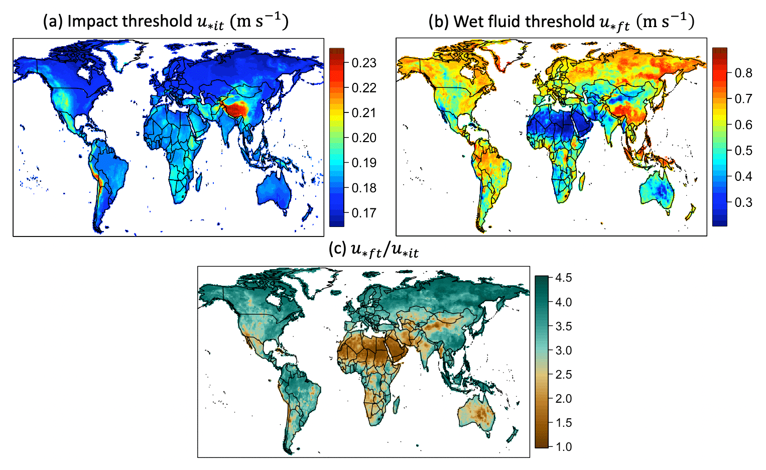
Figure 5 The dust emission thresholds using the Shao and Lu (2000) scheme for the year 2006 on a 0.5^∘ × 0.625^∘ grid. (a) The impact threshold u_∗it calculated using ${\stackrel{\mathrm{‾}}{D}}_{\mathrm{p}\mathrm{0}}=\mathrm{127}\mathit{\mu }\mathrm{m}$ (Eq. 4), (b) the wet fluid threshold u_∗ft (Eq. 1), and (c) the ratio between the wet fluid threshold and impact threshold which is $f_{\mathrm{m}}/\mathrm{0.81}$, where f_m is the moisture effect on u_∗ft (Eq. 3). The larger this ratio, the wider the range of wind speeds for which hysteresis in dust emission occurs, and the more important it is to account for intermittency in dust emissions.

Figure 6a shows the 2006 annual mean intermittency effect over the Bodélé Depression as an example. Figure 6a shows hourly mean η as a function of the hourly mean u_s. It demonstrates the properties of η discussed above: e.g., when u_s>u_ft, η→1 and when u_s<u_it, η→0. In both regimes, the behavior of the dust emission intermittency is asymptotic to dichotomous (0 or 1) activity which is the same as that of the conventional emission schemes. Near the intermittency or hysteresis regime $u_{\mathrm{it}}<u_{\mathrm{s}}<u_{\mathrm{ft}}$, η is intermediate between zero and 1, and thus a scheme using u_∗it gives a small finite emission flux while conventional schemes using u_∗ft give a prediction of zero. The color code shows the strength of convection $-z_i/L$. $-z_i/L$ is positive (red) when buoyant convection is active (L<0) and is negative (blue) when the PBL is statically stable (L>0). The color shows that there is a modest correlation between $-z_i/L$ and u_s, but the correlation is not necessarily strong, and the strongest buoyancy (dark red) often happens when u_s (or shear u_∗s) is moderate. The strongest buoyancy associates with moderate η values of ∼ 0.5 only, and for the highest η values $-z_i/L$ is mildly unstable (light red). This means that the turbulent fluctuation is primarily governed by shear u_∗s instead of controlled by buoyancy $-z_i/L$, and the intermittency behavior is dictated by shear-driven instead of buoyancy-driven turbulence. Equation (23) could essentially be simplified into ${\mathit{\sigma }}_{{\stackrel{\mathrm{̃}}{u}}_{\mathrm{s}}}\approx {\mathrm{12}}^{\mathrm{1}/\mathrm{3}}{u}_{\ast \mathrm{s}}$.

Figure 6b shows the global spatial distribution of the annual mean η for the year 2006, averaged across time steps during which saltation and dust emissions are occurring over the grid (and thus η during time steps when F_d=0 is not counted). Most marginal sources have small η<0.3 (red color), indicating dust emissions are fluctuating and intermittent. These emissions may not be existent in other LSMs employing u_∗ft in the dust emission equation (but also dependent on their threshold tuning). Over these regions, because of the intermittent shut-offs of emissions, the emissions need to be scaled down by the fraction of time η which is also missed by other LSMs. Intermittency is thus critical in accounting for emissions over semiarid regions. Regions with high η (more continuous emission; light blue color) include El Djouf; the Bodélé Depression; the Libyan–Nubian Desert over Libya, Egypt, and Sudan; the Rub' al Khali Desert within the greater Arabian Desert; the Lut Desert in Iran; the Taklamakan Desert; and the Strzelecki Desert in Australia. During saltation, these regions tend to have wind episodes further away from the thresholds, leading to a high η. However, regions with high η are not necessarily regions with the highest dust emissions (Fig. 7a–b) because their saltation frequency could be low, or the strength of their emission fluxes is limited by other factors such as the fragmentation exponent and soil moisture. In Fig. S5, we further show the factor η averaged over all time steps of 2006, including periods of no emissions over the grid. Since η is close to 0 when there is no emission, Fig. S5 shows much smaller η compared to Fig. 6b.

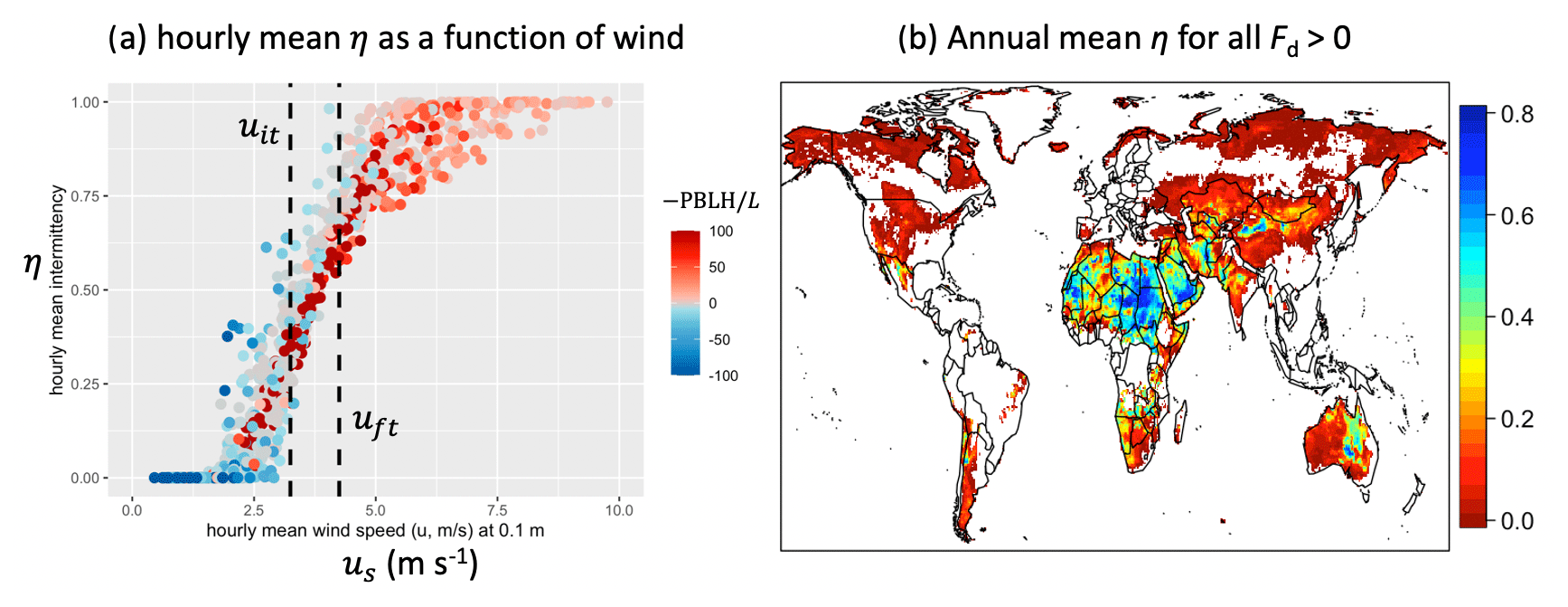
Figure 6 Simulated dust emission intermittency effect for the year 2006. (a) The hourly mean intermittency factor η versus hour mean wind speed u_s (m s⁻¹) at 0.1 m height over the Bodélé Depression. The color indicates $-z_i/L$, with red indicating $-z_i/L>\mathrm{0}$ (unstable), blue indicating $-z_i/L<\mathrm{0}$ (stable), and gray indicating $-z_i/L\sim \mathrm{0}$ (neutral). The two vertical dotted black lines indicate the annual mean impact threshold (left) and the fluid threshold (right) wind speed (m s⁻¹) at 0.1 m. (b) The annual mean intermittency factor η, or equivalently the fraction of time within a time step that emission is active, averaged over times when emission is active (F_d>0).

4 Results of our new dust emission scheme

In this section, we implement the three new parameterizations of key dust emissions processes with the K14 model into R to investigate the resulting spatial variability of dust emissions. The MERRA-2 data and ESA CCI land cover data are for the year 2006. Other inputs in Table 1 (SoilGrids data, Prigent's roughness, and source functions) are 2-D spatial datasets with no 2006 data available, but they are slowly time-varying variables and are generally used for present-day simulations in other years. In Sect. 4.1, we then compute the dust emissions and analyze their spatial characteristics. We examine the effects of each new modification on the simulated dust emissions by conducting different simulations with different individual parameterizations added. Then, in Sect. 4.2, we inspect the effects of the grid resolution of input data on simulating dust emissions and propose a simple method to calibrate the spatial variability of low-resolution dust emissions to match the spatial variability of high-resolution emissions.

4.1 Effects of different new physics on global dust emissions

In this subsection, we show the effects of different modifications on the resulting dust emissions (in kg m⁻² yr⁻¹) in Fig. 7. We demonstrate the effect of each modification by creating a suite of sensitivity experiments as follows: (I) first we simulate emissions using the default K14 scheme, (II) then we use the K14 scheme with our proposed globally constant soil diameter of ${\stackrel{\mathrm{‾}}{D}}_{\mathrm{p}\mathrm{0}}\sim \mathrm{127}$ µm for simulation, (III) we further add in the hybrid drag partition physics on top of (II), (IV) we switch from using the fluid threshold to the impact threshold in (III), and finally (V) we include the intermittency effect on top of (IV) for simulation. We note that past studies derived the approximate magnitude of the global total emission (e.g., Tegen and Fung, 1995; Zender et al., 2004; Evan et al., 2014; Kok et al., 2021), but there are no global observations of dust emissions. In the field of dust modeling, there are currently no first principles that can derive the essential dust emission proportionality constants to constrain modeled emissions at a correct order of magnitude, which means scientists still have insufficient knowledge in aeolian physics to generate emissions predictions in the correct order of magnitude. Recognizing that the spatiotemporal characteristics of the predictions are more credible, it is very common for dust modelers to rescale the emissions according to the known constraints of observed atmospheric dust mass or the global DAOD. For instance, Li et al. (2022) scaled all their simulations to achieve a global mean DAOD of 0.03, based on Ridley et al. (2016). Thus, what matters the most is how each modification changes the spatial variability and the relative magnitudes of dust emitted from one region compared to the others, and the absolute magnitude changes are of secondary importance. In our experiments, we normalize all simulations to a global total of 5000 Tg yr⁻¹, which is around the current constraint of global PM₂₀ dust emission flux from past studies (Evan et al., 2014; Kok et al., 2021a, b). Figure 7 shows the normalized emissions of K14 and our scheme (Fig. 7a–b) and differences between the normalized emissions from one modification to another (Fig. 7c–j). The left panels (Fig. 7c, e, g, i) show the normalized emission differences, and the right panels (Fig. 7d, f, h, j) show the normalized emission ratios. The left columns show the regions with the greatest changes in absolute magnitude, which would mostly be dominated by hyper-arid regions and primary sources, whereas the right columns show the regions with the biggest percentage changes with respect to their own order of magnitude. Figure S6 shows the original, unnormalized emission maps for all experiments, and Fig. S7 shows the differences in unnormalized emissions between different experiments. Figure S8 shows the normalized emission maps for all experiments. Table S2 summarizes the global total changes in the normalized emissions done by all modifications.

Figure 7a shows the normalized emissions from the default K14 scheme (experiment I) using MERRA-2 inputs. The emission map shows a similar spatial pattern compared with the K14 simulations in Kok et al. (2014b) and Li et al. (2022) despite differences in the data used for different land-surface fields (e.g., for LAI and soil moisture) and a larger LAI limit of 1 used in this study. The most significant emissions are over the Bodélé Depression in Chad, the Nubian Desert in Sudan and Egypt, the whole Arabian Peninsula, most of Iran, the Taklamakan Desert in China, and the Strzelecki Desert in Australia. Over regions with emissions, the spatial variability of the emissions is dictated by the moisture w (see Figs. S1 and 5b), which fundamentally shapes the threshold u_∗ft, the soil erodibility C_d, and the intermittency η. Smaller emissions occur over southern Africa, South America, and the western United States. Without normalization, the simulated emissions in Fig. S6a gives a global total of ∼ 29 300 Tg yr⁻¹ using the inputs in Table 1.

Figure 7c–d show the effect of changing the global soil diameter from the current standard of 75 µm to our new constraint of ${\stackrel{\mathrm{‾}}{D}}_{\mathrm{p}\mathrm{0}}=\mathrm{127}$ µm (experiment II). As described in Sect. 3.1, a globally larger ${\stackrel{\mathrm{‾}}{D}}_{\mathrm{p}}$ leads to heavier particles, resulting in higher thresholds and lower emissions across the globe. Figure 7c shows that the normalized emission tends to redistribute from semiarid regions to hyper-arid regions, but the changes are small overall. The color bar in Fig. 7c shows that the effect of employing a new global ${\stackrel{\mathrm{‾}}{D}}_{\mathrm{p}\mathrm{0}}$ is relatively mild (of the largest order of 0.001 kg m⁻² yr⁻¹) compared to the drag partition effect and intermittency (Fig. 7e and g; of the largest order of ∼ 0.1 kg m⁻² yr⁻¹). Figure 7d shows the ratio map of the normalized emissions of experiment II to those of experiment I. Employing a new globally constant ${\overline{D}}_{p\mathrm{0}}$ does not strongly impact the spatial pattern of the emissions, so the ratio map is of order 1 around the globe. While Fig. 7c more clearly shows that the largest emission changes in magnitude occur over the major sources, Fig. 7d shows that, after rescaling, there are some stronger emissions reductions in percentage (in blue) over marginal regions (e.g., the Arctic) compared to the minimal increases over the major sources (in white and light red, e.g., over the Bodélé Depression). The major sources are less affected, since in the high u_∗s regime F_d becomes more sensitive to u_∗s than to u_∗ft. Thus, a uniform increase in u_∗ft around the globe tends to eliminate small emissions more than large ones. The main effect of employing a larger ${\stackrel{\mathrm{‾}}{D}}_{\mathrm{p}}$ is therefore a very modest shift of emissions from the marginal regions toward the arid areas. Summing up the absolute magnitude of changes in Fig. 7c, out of 5000 Tg yr⁻¹ there are 250 Tg yr⁻¹ of dust redistributed within source regions. Figure S6b shows the unnormalized global emission flux of ∼ 23 900 Tg yr⁻¹, which is 18 % less than the unnormalized emission flux of experiment I as a result of globally increased thresholds. We note that the difference maps of unnormalized emissions in Fig. S7a show that larger emissions reductions occur over the major sources just because the emission magnitudes are larger there.

Figure 7e–f show the effect of including the hybrid drag partition effect F_eff (experiment III). The clear contrast between major and marginal sources is shown in Fig. 7e and f, which mirrors the spatial pattern of F_eff in Fig. 4c. Compared with experiment II, experiment III has emissions redistributed from semiarid to hyper-arid regions, since the drag partition effect leads to stronger inhibitions of emissions over the nonarid regions than the arid regions. For example, normalized emissions increase (in red) over major sources such as the Bodélé Depression, El Djouf, and the Rub' al Khali Desert; normalized emissions over the western United States and western Australia are significantly reduced. El Djouf is a significant dust source over Africa (Yu et al., 2018), yet K14 fails to represent its high emissions because of the strong moisture effect (see Fig. 5c) compared to other major sources such as the Bodélé Depression. However, F_eff highlights El Djouf as a highly erodible surface and helps mitigate the low emission issue over there. Similarly, the underrepresented emissions over the Taklamakan and the Arabian Desert by K14 are partially mitigated by accounting for the drag partitioning (light red in Fig. 7f). Summing up the absolute magnitude of changes in Fig. 7e, out of 5000 Tg yr⁻¹ there is 3611 Tg yr⁻¹ of dust redistributed within the source regions. This shows that the drag partition effect has a much bigger influence on the spatial variability of dust emissions than changing ${\stackrel{\mathrm{‾}}{D}}_{\mathrm{p}}$ in Fig. 7c. For unnormalized emissions, the global total emission in experiment III decreases drastically by 85 % to ∼ 2880 Tg yr⁻¹ relative to that of experiment II. In Fig. S7b, many significant emissions reductions (in dark blue) occur over the Sahara where F_eff<0.7, such as Egypt, Sudan, and the western Sahara. K14 struggles to distinguish major sources (e.g., the Bodélé) from less significant sources (e.g., Sudan) and predicts similar levels of emissions. F_eff effectively introduces the effect of surface roughness on mitigating emissions over secondary sources, reducing the emissions by at least 1 order of magnitude compared to Fig. S6b.

Figure 7g–h show the effects of implementing the C19 intermittency scheme. It consists of employing u_∗it in K14 (experiment IV) and further multiplying the dust emission flux by the intermittency factor η (experiment V). Figure 7g–h show their combined effects by comparing experiment V with experiment III. As seen from Fig. 7g and h, emission schemes employing u_∗it will have much stronger emissions over marginal sources. This is because not only is $u_{\ast \mathrm{ft}}/u_{\ast \mathrm{it}}$ bigger but the fragmentation exponent κ (which scales with u_∗ft) is also greater over marginal sources. As a result, the main feature in the spatial pattern of Fig. 7h is that the marginal sources (in red color) now have more emissions than experiments II and III. The most apparent emissions increases are over Patagonia, the Horn of Africa (HOA), and western US deserts. Another observable change is that there are many more high-latitude dust emissions, such as over the Arctic, Canada, and Alaska. Studies reported that many models greatly underestimate high-latitude dust emissions (Bullard et al., 2016; Meinander et al., 2022), and the use of u_∗it will mitigate this issue. Figure 7g shows that although the changes over nonarid regions are high in ratios (e.g., >1000 times over Canada in Fig. 7h), the emission redistributions in magnitude are still small (e.g., ∼ 10⁻⁵ kg m⁻² yr⁻¹ in Canada) compared to the major sources (e.g., $>{\mathrm{10}}^{-\mathrm{3}}$ kg m⁻² yr⁻¹ in the Sahara) because the magnitudes in experiment III are too small over nonarid regions. The unnormalized total emissions (Fig. S6d) vastly increase to ∼ 13 200 Tg yr⁻¹ when employing u_∗it instead of u_∗ft, more than 4 times that of experiment III.

On the other hand, the effect of multiplying the emission flux with the intermittency factor η is less dramatic than the effect of using u_∗it. η tends to scale down small emissions (Fig. 5b), so fluxes from major sources are only moderately reduced. In contrast, fluxes from marginal source regions (e.g., high-latitude boreal forests) are typically reduced by ∼ 1–3 orders of magnitude (blue areas in Fig. S6e). However, experiment V has a global total of ∼ 11 700 Tg yr⁻¹, which is only 11 % smaller than experiment IV, because those remote regions as such already have small emissions. All in all, accounting for both the impact threshold and the intermittency factor will increase the global total emission from ∼ 2880 Tg yr⁻¹ in experiment III to ∼ 11 700 Tg yr⁻¹ in experiment V, which is about a 4-fold increase. Figure 7h shows that C19 mainly increases marginal emissions; the overall effect of C19 is thus to move emissions from the hyper-arid regions to semiarid regions. Summing up the absolute magnitude of changes in Fig. 7g, out of 5000 Tg yr⁻¹ there is 3163 Tg yr⁻¹ of dust redistributed within the source regions, indicating that the intermittency scheme induces a similar magnitude of changes compared to employing F_eff. Both the hybrid drag partition scheme and the intermittency scheme lead to >60 % of dust emissions redistributed, showing that both effects modify the modeled emission behavior much more strongly compared to the effect of changing the value of ${\stackrel{\mathrm{‾}}{D}}_{\mathrm{p}}$ (experiment II).

Figure 7b shows the final emission map of our new dust emission scheme with all new physics, and Fig. 7i–j shows the resulting emission changes and ratios from K14 (experiment I) to our scheme (experiment V). Figure 7i–j show that compared to K14, our scheme's emission fluxes over densely vegetated regions (e.g., equatorial Africa and northern Australia) are reduced due to the drag partition effect, while there are increases in marginal sources like the Arctic and mid-latitude boreal forests due to the intermittency effect. The figures show essentially a combination of drag partition (Fig. 7e–f) and intermittency (Fig. 7g–h) effects. Major sources are more affected by the drag partition effect (e.g., the Bodélé Depression and El Djouf), while marginal sources are more dominated by turbulence and intermittency (e.g., the Arctic). For regions where both effects take place, more vegetated semiarid regions are more affected by the drag partition (e.g., western United States), while less vegetated semiarid regions are more affected by the intermittency (e.g., Patagonia, the Great Plains of the United States, and southern Australia). For unnormalized emissions, our scheme's global total of 11 700 Tg yr⁻¹ is ∼ 60 % smaller than the K14 emission. A notable feature is that the new mechanisms favor the emissions over the Horn of Africa (HOA) the most, with an emission increase of ∼ 2 kg m⁻² yr⁻¹ (as seen in Figs. 7g and S7f). This is because in C19, the HOA has low u_∗it, high summertime u_∗, low roughness element cover (and thus high F_eff), and moderate soil moisture (and thus high dust emission coefficient C_d). This issue could be problematic, since it could introduce too much dust in the GCM over the HOA, which is further discussed in Sect. 5.

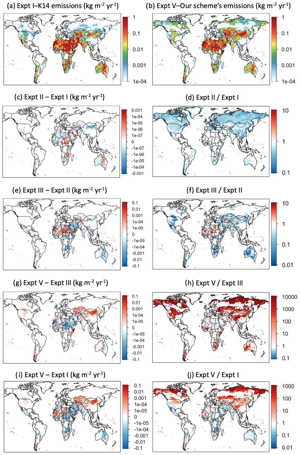
Figure 7 The effects of the proposed improvements to the parameterization of dust emissions on the default Kok et al. (2014a, b) dust emission scheme. (a, b) Globally normalized dust emission fluxes simulated by (a) the default K14 scheme (expt. (experiment) I) and (b) our new scheme (expt. V). (c–j) Maps of normalized emission (c, e, g, i) differences and (d, f, h, j) ratios, with individual improvements added on top of the default K14 scheme. The individual improvements are respectively (c, d) changing the soil median diameter to 127 µm (expt. II), (e, f) including the drag partition effect (expt. III), and (g, h) employing the Comola et al. (2019) intermittency scheme (expt. V). (i, j) Maps of (i) normalized emission differences and (j) emission ratios for our new scheme and the K14 scheme. The color bars of the maps of differences are drawn to log₁₀ scale.

4.2 The grid-scale dependence of our new dust emission scheme

The spatial resolution of a GCM strongly affects the budget and spatiotemporal variability of dust emissions because modeled emissions scale nonlinearly with input meteorological fields (Ridley et al., 2013; Meng et al., 2021). Many current GCMs have a horizontal resolution of ∼ 1–2^∘ (Zhao et al., 2022). Most of the datasets employed in this paper, such as the 0.5^∘ MERRA-2 fields and the even finer aeolian roughness length z_0a, are datasets of higher horizontal resolutions. Thus, GCMs need to regrid the datasets to the model native grid resolution as model input. Since dust emission has nonlinear dependences on multiple variables such as u_∗ and w, using a simple, area-weighted spatial average of u_∗ to calculate dust emission would be inaccurate, as it is different from an area-weighted average of high-resolution dust emissions per se, i.e., for any n>1 ${\stackrel{\mathrm{‾}}{u}}_{\ast \mathrm{s}}^n<\stackrel{\mathrm{‾}}{u_{\ast \mathrm{s}}^n}$ leads to $F_{\mathrm{d}}\left({\stackrel{\mathrm{‾}}{u}}_{\ast \mathrm{s}}^n\right)<\stackrel{\mathrm{‾}}{F_{\mathrm{d}}\left(u_{\ast \mathrm{s}}^n\right)}$ (Ridley et al., 2013) (here we use the bar as a spatial average from a finer to a coarser grid). This inequality applies to our model and datasets as well: simply taking the area-weighted mean of high-resolution u_∗s or w in a model grid box will omit the locally high u_∗s (or low w) values that can produce locally extremely high emissions, resulting in an underestimation of emissions relative to direct area-weighted averaging of the emissions. Additionally, the presence of thresholds in dust emission parameterizations further intensifies the scale dependence, because spatially averaging u_∗s might cause ${\stackrel{\mathrm{‾}}{u}}_{\ast \mathrm{s}}<{\stackrel{\mathrm{‾}}{u}}_{\ast \mathrm{it}}$ which leads to zero emission over a coarse grid box, whereas fine emissions could be large than zero when $u_{\ast \mathrm{s}}>u_{\ast \mathrm{it}}$ in any fine grid. Dust emission flux will thus be strongly dependent on model resolution more than other linear processes (Zender et al., 2003a; Ridley et al., 2013; Meng et al., 2021), which is undesirable. There is a need to better upscale low-resolution dust emissions to match the variability of high-resolution emissions such that dust emissions tend to be less resolution dependent. To address the problem of missing emissions due to the smoothing of the subgrid wind maxima, a common approach is to employ a grid-by-grid Weibull distribution to the GCM winds to represent the subgrid wind maxima and thus obtain the subgrid emission peaks (Cakmur et al., 2004; Grini et al., 2005; Cowie et al., 2015; Zhang et al., 2016; Menut, 2018; Tai et al., 2021). However, the shape factor of the distribution needs to be empirically determined and thus might not capture the interannual variability and changes in climate. In this subsection, we examine the scale dependence of our dust emission scheme and then propose an alternative approach, which is to derive a simple spatial map and upscale the spatial variability of dust emissions from low-resolution ones to high-resolution ones. A discussion about our proposed approach versus the more common Weibull distribution approach is detailed in Sect. S6.4.

We first examine the scale dependence of our dust emission scheme. We achieve this by performing an area-weighted mean of all input meteorological and land-surface variables to various coarser resolutions. Starting from the native 0.5^∘ × 0.625^∘ resolution of MERRA-2, we regrid fields to 0.9^∘ × 1.25^∘, 1.9^∘ × 2.5^∘, and 4^∘ × 5^∘. Then we use these input fields with our new scheme to compute hourly dust emissions for 2006 across these four resolutions. We then compare the emission outputs across these resolutions.

We examine the global, regional, and grid-level scale dependence of our dust emission scheme in Fig. 8. At the regional level, Fig. 8a shows the unnormalized annual total emissions (in Tg yr⁻¹) of nine major dust source regions. The source regions are defined following Kok et al. (2021a) (see Figs. S9 and 8c–d). The regional dust abundance in Fig. 8a is mainly consistent with the regional dust emissions in Kok et al. (2021b; see their Fig. 2). The highest emissions occur over the Middle East/Central Asia, followed by the Sahel and northern Africa. Smaller emissions are over East Asia, North and South America, Australia, and southern Africa. The dust emission scheme also shows scale dependence across different resolutions. Some regions may have a sharper decrease in emissions from 0.9^∘ × 1.25^∘ to 1.9^∘ × 2.5^∘ (e.g., northeastern Africa), and some regions may have a sharper decrease from 1.9^∘ × 2.5^∘ to 4^∘ × 5^∘ (e.g., Sahel). This difference is contingent upon the degree of smoothing of the input fields such as u_∗s at a particular resolution. The emissions will drastically drop when the local extrema of u_∗s are smoothed out and no longer can be represented at a particular resolution, and over different regions this cutoff may occur at different resolutions depending on the spatial heterogeneity of the local-scale meteorological fields. Nevertheless, in general, the coarser the resolution, the worse the model can represent the local variability of u_∗s and other input fields and subsequently the emissions, and thus the magnitudes of the emissions decrease with resolution. Figure 8a shows that the relative differences in regional emissions can be different in different resolutions (e.g., Sahel can have larger emissions than the Middle East/Central Asia in the 4^∘ × 5^∘ simulation), which will subsequently affect the spatial variability of other major dust cycle variables (such as DAOD or deposition). Therefore, it is always preferential for GCMs to simulate the dust cycle in high resolutions. Figure 8b shows the scale dependence of the global emissions, which also shows the same decrease in emissions from fine to coarse grid resolutions.

We also examine the scale dependence of dust emissions at the grid level. Figure 8c–d show the spatial distributions of 0.5^∘ × 0.625^∘ and 1.9^∘ × 2.5^∘ unnormalized emissions (with a global total of 11 700 and 5450 Tg yr⁻¹, respectively). The 0.5^∘ × 0.625^∘ simulation shows a more detailed local spatial variability compared to the coarser 1.9^∘ × 2.5^∘ simulation. The 1.9^∘ × 2.5^∘ simulation fails to capture some of the high emission regimes in the 0.5^∘ × 0.625^∘ simulation such as over the Taklamakan, and it fails to simulate the local emission peaks over marginal sources such as the Chihuahuan Desert and Patagonia. Coarse-gridded simulations lose emissions in both major and marginal dust sources. We calculate in Fig. 8e the grid-by-grid ratio of unnormalized 0.5^∘ × 0.625^∘ emissions to 1.9^∘ × 2.5^∘ emissions to show the emissions missed by the 1.9^∘ × 2.5^∘ simulation in each grid. Both the coarse (y axis) and fine (x axis) emissions are plotted in the log₁₀ scale to show the emission ratios in terms of the order of magnitude only. It can be seen that most of the points are above the 1:1 line (dashed black line), meaning the coarse emissions are underestimating some local dust fluxes accounted for by the fine emissions. The low-resolution simulation can capture the largest emissions well (top righthand corner), as predicted by the high-resolution simulation. However, the smaller the emission, the more significant the difference in emissions, and for minimal emissions ($<{\mathrm{10}}^{-\mathrm{5}}$ kg m⁻² yr⁻¹), the difference can be up to 3 orders of magnitude. There are very few grids with low-resolution emissions higher than high-resolution emissions. Those are exceptional cases due to the spatial variability of moisture w more heterogeneous than that of u_∗s, leading to the smoothing of local maxima of u_∗ft instead of u_∗s and thus the overestimation of F_d in the coarser simulation. In conclusion, the coarse-resolution models omit many local input features and thus fail to represent the correct spatial variability of dust emissions.

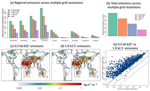
Figure 8 The dependence on horizontal resolution of dust emissions simulated with our new dust emission scheme. (a, b) Bar plots of dust emissions as a function of grid resolutions for (a) nine major dust emission regions and (b) the globe. (c) Unnormalized emissions of 0.5^∘ × 0.625^∘ and (d) 1.9^∘ × 2.5^∘. (e) A scatterplot of 0.5^∘ × 0.625^∘ versus 1.9^∘ × 2.5^∘ unnormalized dust emissions. The rectangular boxes show the nine source regions in (a) defined as in Fig. S9.

To mitigate the scale dependence of our dust emission simulations, here we propose a simple approach to upscale the simulated low-resolution emissions to match the high-resolution emissions. This approach assumes that the fine emissions have a more adequate magnitude and spatiotemporal variability than the coarse emissions so that the coarse emissions are calibrated to match the fine emissions. Our approach is that, by dividing the normalized fine-resolution emission map F_d,f by the coarse-resolution emission map F_d,c, we obtain a map of scaling factors ${\stackrel{\mathrm{̃}}{K}}_{\mathrm{c}}$ to account for the differences in the spatial variability of dust emissions between high- and low-resolution simulations:

$$\begin{array}{}\text{(24)}& {\stackrel{\mathrm{̃}}{K}}_{\mathrm{c}}\left(\mathrm{long},\mathrm{lat}\right)=F_{\mathrm{d},\mathrm{f}}\left(\mathrm{long},\mathrm{lat}\right)/F_{\mathrm{d},\mathrm{c}}\left(\mathrm{long},\mathrm{lat}\right).\end{array}$$

We obtain a global map of correction factors ${\stackrel{\mathrm{̃}}{K}}_{\mathrm{c}}$ and apply this map to all simulated coarse emissions from both historical and future simulations, correcting their spatial variability to match that of the high-resolution emissions. We show the seasonal variability of ${\stackrel{\mathrm{̃}}{K}}_{\mathrm{c}}$ in Fig. S10. This map of scaling factors contains some temporal and seasonal variability, so it would be preferable to apply a seasonally varying dataset of ${\stackrel{\mathrm{̃}}{K}}_{\mathrm{c}}$. However, ${\stackrel{\mathrm{̃}}{K}}_{\mathrm{c}}$ varies modestly across season because the subgrid variability of the meteorological and land-surface fields is partly determined by spatial structures such as orography or land use/land cover, which change across a relatively long enough timescale (decadal to multidecadal or longer). We note that theoretically this approach will fail to work if, over the remote regions, the low-resolution emission is zero throughout the entire simulation period while the high-resolution emission is a small positive definite, since ${\stackrel{\mathrm{̃}}{K}}_{\mathrm{c}}$ will go to infinity. We also note that employing different input fields or different emission schemes will change the subgrid variability and thus the spatial representation of this correction map. For instance, one will obtain a slightly different correction map if one uses ERA-Interim meteorology instead of MERRA-2 or a moderately different map if one employs the Z03 or any other dust emission equations instead of K14 or our new scheme. Therefore, although here we present a standard correction map which is likely accurate and realistic, we suggest each model should make their own correction maps for their specific model configurations. We discuss more caveats of this approach in Sect. 5.4.

Figure 9 shows the ratio maps normalized fine emissions to coarse emissions. Figure 9a shows the ratio of normalized 0.5^∘ × 0.625^∘ emissions (F_d,0.5) to constrained 1.9^∘ × 2.5^∘ emissions (F_d,2), and Fig. 9b shows the ratio of constrained F_d,0.5 to constrained 0.9^∘ × 1.25^∘ emissions (F_d,1). Since all emissions are constrained to match the global dust budget, the correction maps display the relative changes in spatial variability between two resolutions. From Fig. 9a–b, it can be seen that 0.5^∘ × 0.625^∘ emissions tend to generate relatively fewer emissions (blue color) over the major sources, such as the Sahara, the Arabian Desert, and the Taklamakan Desert. Emissions of 0.5^∘ × 0.625^∘ also tend to have relatively more emissions (red color) over the peripheries of the major sources, such as Algeria, Yemen, and the Taklamakan. This is in line with the above discussion, because the high-resolution simulations tend to be more capable of representing the local peaks of u_∗s and therefore can more likely pass the thresholds and produce F_d; the low-resolution simulations would miss a lot of marginal emissions because the low-resolution wind will be smaller than the low-resolution threshold and yield a zero F_d. The ratios over the marginal sources can be up to 100 or even more because of the much smaller emissions in low-resolution simulations. The contrast is smaller (with ratios of 0.5–0.9) over major sources where coarser simulations are more capable of representing the large-scale emission fluxes. For this reason, the correction values in Fig. 9a for 1.9^∘ × 2.5^∘ (${\stackrel{\mathrm{̃}}{K}}_{\mathrm{c},\mathrm{2}})$ generally have bigger magnitudes than those in Fig. 9a for 0.9^∘ × 1.25^∘ (${\stackrel{\mathrm{̃}}{K}}_{\mathrm{c},\mathrm{1}})$. These maps indicate that in coarse-gridded simulations, dust emissions are overall underrepresented over marginal sources and overrepresented over major sources. Therefore, we propose implementing these maps into GCMs of ∼ 1^∘ or coarser resolution to correct the dust emission spatial variability accordingly. Scaling all simulations across different spatial resolutions to the finest spatial resolution will move our dust emission scheme toward a scale-aware and grid-independent formulation.

Figure 9 Gridded maps of a 0.9^∘ × 1.25^∘, 1.9^∘ × 2.5^∘, and 4^∘ × 5^∘ scaling factor to rescale the coarse dust emission simulations to match the spatial variability of high-resolution dust emissions. This is achieved by calculating the ratios of (a) 0.5^∘ × 0.625^∘ to 1.9^∘ × 2.5^∘ emissions, (b) 0.5^∘ × 0.625^∘ to 0.9^∘ × 1.25^∘ emissions, and (c) 0.5^∘ × 0.625^∘ to 4^∘ × 5^∘ emissions. Emissions of all resolutions are constrained and normalized to have a global total of 5000 Tg yr⁻¹ before calculating the ratios.

4.3 Comparison of our dust emission scheme against other dust estimates

To validate the emissions produced by our new scheme, this subsection focuses on comparing the resulting 0.5^∘ × 0.625^∘ emissions from our new scheme against other existing emission data. Since there are no globally gridded observations of dust emissions, GCMs and ESMs mostly evaluate their schemes using observable atmospheric dust products such as satellite and ground-based DAOD data, as well as dust surface concentrations and dust deposition flux measurements (Ridley et al., 2012; Kok et al., 2014b; Pu and Ginoux, 2018; Parajuli et al., 2019; Klose et al., 2021). Since this study focuses on simulating dust emissions, not their subsequent transport and deposition, we compare our results against constraints on the fraction of annual dust emission contributed by nine major source regions (Table 1 in Kok et al., 2021b). These constraints on regional emission fluxes were obtained from the Dust Constraints from joint Observational-Modelling-experiMental analysis (DustCOMM) dataset (Kok et al., 2021a, b), which used inverse modeling to combine an ensemble of model simulations of the global dust cycle with constraints on the regional DAOD near major dust source regions (Ridley et al., 2016), the dust size distribution (Adebiyi and Kok, 2020), and dust extinction efficiency (Kok et al., 2017). The DustCOMM constraints on regional dust emissions include error estimates that account for the spread in model results and the uncertainties in the constraints on dust properties and abundance. Comparisons against independent measurements of dust surface concentrations and deposition fluxes indicated that the DustCOMM product is more accurate than GCM simulations and the MERRA-2 dust reanalysis and that uncertainties are realistic (Kok et al., 2021a, b). The total emissions from all nine source regions obtained by the DustCOMM dataset were 4.7 (3.4–9.1) × 10³ Tg yr⁻¹ for dust PM₂₀. The global total of ∼ 4700 Tg yr⁻¹ is close to the 5000 Tg yr⁻¹ we adopted in this study for normalization, and we again normalized the DustCOMM global emissions to 5000 Tg yr⁻¹. Note that Kok et al. (2021a, b) only constrained the emissions and other dust variables for each broad region, but its subregional spatial distribution of dust is a multimodel mean and thus unconstrained. Therefore, in Fig. 10b, we sum up the emissions of DustCOMM to regional total emissions, which are constrained by the regional DAOD from Ridley et al. (2016). We also sum up the emissions of all other schemes to regional levels to evaluate each scheme's regional spatial variability against DustCOMM. Tables S3 and S4 summarize the global total emissions and regional emissions of DustCOMM and all other schemes.

We first compare the global emission maps between DustCOMM and different schemes. Figure 10a shows the gridded global spatial distribution of DustCOMM dust emissions (Kok et al., 2021a). Here we compare the gridded simulations of K14 (Fig. 7a) and our scheme (Fig. 7b) against the gridded K21 DustCOMM emissions. Our new scheme's simulation successfully captures most of the major peaks in DustCOMM emissions, except that there are more northern US and high-latitude emissions in our new scheme which were not represented and constrained in DustCOMM's inverse analysis. Our scheme and DustCOMM emissions have a gridded spatial correlation coefficient of r=0.71, showing the resemblance of the two emission maps and our scheme's ability in physically capturing the emission peaks. On the other hand, K14 emissions also share a similar spatial distribution with DustCOMM emissions but show more emissions over central Africa, central India, and northern Australia. Its gridded spatial correlation coefficient with DustCOMM is r=0.61, indicating it does not match DustCOMM emissions in spatial variability as well as our scheme does.

We also conducted simulations using the Z03 scheme (Eq. 10) for comparison with our scheme's simulation. The Z03 scheme requires a source function S, and in this study we adopted two popular source functions: one is the Zender et al. (2003b) geomorphological source function (e.g., used in CESM; Oleson et al., 2013) and the other one is the Ginoux et al. (2001) source function (e.g., used in GEOS-Chem; Fairlie et al., 2007). Both source functions are plotted in Fig. 2 in Kok et al. (2014b). Figure S11a shows the simulations of the Z03 scheme with Ginoux et al. (2001) S (Z03–G), which shows almost an identical pattern with the Z03–G scheme in the GEOS-Chem simulations (e.g., top panel of Fig. 1 in Meng et al., 2021). The Z03–G scheme is mostly consistent with the DustCOMM multimodel emissions (r=0.57) but captures more African emissions in the northwest Africa such as Algeria, Morocco, and the western Sahara. On the other hand, the Z03–Z scheme employs a geomorphic S that possesses a spatial distribution of the upstream area where surface runoff is collected, from Zender et al. (2003b). Figure S11b shows the simulations of the Z03–Z scheme, which shows a highly similar pattern with the Z03–Z scheme in the CESM simulations (e.g., Fig. 2a in Li et al., 2022). It captures the emission peaks across the globe but is quite spatially heterogenous, yielding a relatively low r=0.35 with DustCOMM.

We further obtained MERRA-2-simulated dust emissions for comparison. MERRA-2 simulates the dust cycle using the global ozone chemistry aerosol radiation and transport (GOCART) model, which employs the Ginoux et al. (2001) scheme (hereafter G01). We thus use MERRA-2-simulated dust emissions here for a comparison between G01, Z03, K14, our scheme, and DustCOMM. However, since DustCOMM employs GOCART dust as one of the six models for inverse analysis and assimilation (see Table 1 of Kok et al., 2021a), and because both DustCOMM and MERRA-2 use remotely sensed aerosol optical depth, DustCOMM and MERRA-2 emissions show relatively similar spatial distributions. Figure S12a shows MERRA-2 annual mean emissions, which show very similar features of grid-by-grid variability especially over Australia, East Asia, and the Middle East. For the same reason, MERRA-2 emissions have a high correlation of r=0.86 with DustCOMM.

Next, we aggregate the emission maps to regional total emissions to examine their regional variability. In Fig. 10b, we compare the simulated dust emissions summed over each of nine source regions against the regional DustCOMM emissions. We also summed the emissions outside all rectangular boxes as the high-latitude emissions, to yield the 10 data points in Fig. 10b. High-latitude emissions from our scheme (Fig. 7b) mainly include emissions from Alaska, Canada, Greenland, and Iceland, and there are no emissions from Antarctica because of the lack of necessary input data there (e.g., soil texture and roughness due to rocks). However, since K21 does not provide emission estimates outside of the nine defined source regions, we compare against the estimate of high-latitude dust emissions from Bullard et al. (2016) (hereafter B16) obtained from GCM results. Their definition of high-latitude emission not only includes emissions from the abovementioned regions but also from Patagonia, so we add Patagonia (39^∘–56^∘ S of S. America) emissions as part of the high-latitude emissions in Fig. 10b. B16 estimated that high-latitude emissions (without error estimates) accounted for 4 %–5 % of their assumed 2000 Tg yr⁻¹ of global total emissions. We normalized their estimate to match our global total of 5000 Tg yr⁻¹, yielding a high-latitude emission range of 200–250 Tg yr⁻¹. We take the average, which is 225 Tg yr⁻¹. For all schemes and datasets discussed here, Table S4 provides a list of regional emission contributions to the global total emission.

Figure 10b shows that our scheme's emissions are in overall better agreement with DustCOMM emissions than the K14 scheme. Some of the most significant differences in emissions between our scheme and K14 are over regions including Australia, North America, and southern Africa, where the vegetation drag partitioning causes strong reductions in winds and emission fluxes (Fig. 7f) from K14 to our scheme. Our scheme's East Asian emission is significantly higher than K14's (also shown in Fig. 7j), primarily due to the switch from using u_∗ft to u_∗it in the dust emission equation (Figs. 7h and S8d). Emissions over South America, the Middle East, and the three regions of northern Africa have relatively small and negligible differences between K14 and our scheme. This occurs because both the drag partitioning and intermittency effects create only minimal changes to the emissions over these regions (Fig. 7j). The results with our scheme (blue color) better match the DustCOMM regional emissions than results with the K14 scheme, lying substantially closer to the 1:1 (black) line over most regions including Africa, Asia, and Australia. There are two notable exceptions where our scheme has less agreement than K14 with DustCOMM, namely North America and the high-latitude emissions. Our scheme generates fewer dust emissions over the Mojave–Sonoran–Chihuahuan deserts over the United States–Mexico border compared to the K14 emissions (Fig. 7a), because of the high LAI (annual mean >0.4) over the western United States that leads to the strong wind drag partitioning. Meanwhile, our scheme generates significant high-latitude emissions over the Arctic, which were not captured by K14 emissions due to the very high u_∗ft. Using the emission intermittency parameterization, our scheme represents one of the earliest attempts to successfully capture significant levels of high-latitude emissions. Our high-latitude emissions account for 262 Tg yr⁻¹ (without Patagonia) and 308 Tg yr⁻¹ (with Patagonia), in total accounting for 5 %–6 % of a global sum of 5000 Tg yr⁻¹, which is very close to the percentage B16 suggested. Our scheme has an R² of 89 % and a root mean squared error (RMSE) of 141 Tg yr⁻¹. We note in Fig. 10b the normalized RMSE (NRMSE) of 28 %, which is the RMSE divided by the mean of the DustCOMM emissions (5000 Tg yr⁻¹/10 data points = 500 Tg yr⁻¹). Our scheme's performance is substantially better than K14's performance with an R² of 65 % and an RMSE = 259 Tg yr⁻¹ (NRMSE = 52 %).

On the other hand, the Z03–Z scheme (Fig. 10c in green) has a similar level of performance compared with K14, with a higher RMSE of 317 Tg yr⁻¹ (NRMSE = 63 %) and an R² of 64 %. The Z03–G simulation (Fig. 10c in violet) has a higher R² of 83 % and also a smaller RMSE of 237 Tg yr⁻¹ (NRMSE = 43 %) against DustCOMM compared with K14 and Z03–Z. Meanwhile, MERRA-2 (Fig. 10d) has a high regional correlation of R² of 88 % and RMSE of 187 Tg yr⁻¹ (NRMSE = 37 %) against DustCOMM regional variability. In conclusion, our scheme outperforms all the aforementioned simulations in matching against the DustCOMM estimates of regional dust emissions.

To evaluate our simulations of the dust emission thresholds, we also compare our simulations of dust emission thresholds against observationally based threshold estimates from Pu et al. (2020). They compared reanalyzed wind speed distributions against observationally derived DAOD distributions to obtain a threshold wind speed for each grid box that corresponds to a threshold DAOD value (e.g., 0.5 over arid regions and 0.05 over semiarid regions), above which is defined as a dust emission event. We show that our simulations of dust emission threshold overall match their derived threshold wind speed in magnitude and spatial variability (see Sect. S5 and Fig. S13).

Figure 10 Dust emissions simulated using different schemes compared against DustCOMM (K21) and Bullard et al. (2016) constraints on regional dust emissions. (a) Globally gridded DustCOMM emissions (kg m⁻² yr⁻¹) based on emissions from six different models that were adjusted using inverse modeling to match constraints on particle size distribution, extinction efficiency, and regional dust aerosol optical depth. The rectangular regions specify the nine source regions defined by Kok et al. (2021a) as also shown in Fig. 8c–d. (b) DustCOMM regional emissions (based on fractional emissions reported in the fifth column of Table 1 in K21b scaled to a global total of 5000 Tg yr⁻¹) versus the regional emissions computed by the K14 scheme and our new scheme. (c, d) Comparison of the DustCOMM regional emissions with the regional emissions computed by the (c) Z03–Z and Z03–G schemes and with (d) MERRA-2 dust emissions. The regional emissions of all simulations are obtained from DustCOMM following the nine source regions in panel (a), with one extra data point representing the high-latitude emissions estimated by Bullard et al. (2016). The error bars show 1 standard error, except that the B16 high-latitude emission does not include an error estimate. The black line shows the 1:1 line.

5 Discussion of the caveats and limitations of the new parameterization

Because of the complexities of simulating the fine-scale process of dust emission in a large-scale gridded model, the parameterizations of dust emission processes presented in Sect. 4 and the dust schemes employed from all past studies necessarily made a number of assumptions. Below, we highlight one important caveat or limitation for each modification made in this paper. We provide discussions on further limitations for each modification in Sect. S6.

For the new dry-soil median diameter ${\stackrel{\mathrm{‾}}{D}}_{\mathrm{p}}$ representation, we used a globally constant ${\stackrel{\mathrm{‾}}{D}}_{\mathrm{p}\mathrm{0}}=\mathrm{127}\pm \mathrm{47}$ µm for calculating dust emission thresholds. In theory, ${\stackrel{\mathrm{‾}}{D}}_{\mathrm{p}}$ should be a function of soil properties (Hillel, 1980) and therefore implicitly a function of space and time, but we obtained a simple relationship for ${\stackrel{\mathrm{‾}}{D}}_{\mathrm{p}}$ over arid regions because (1) there were no statistically significant correlations between ${\stackrel{\mathrm{‾}}{D}}_{\mathrm{p}}$ and standard soil properties like soil texture (Fig. S2), (2) data are insufficient for a detailed statistical analysis against a wider range of soil properties, (3) the uncertainties of soil data are moderately large, and (4) most ${\stackrel{\mathrm{‾}}{D}}_{\mathrm{p}}$ measurements over arid regions found ${\stackrel{\mathrm{‾}}{D}}_{\mathrm{p}}$ within 40–250 µm (Fig. 1c), which limited u_∗ft0 to vary within the relatively small range of ∼ 0.204–0.268 m s⁻¹ (from Eq. 2 assuming ρ_a=1.225 kg m⁻³). Our analysis of a compilation of ${\stackrel{\mathrm{‾}}{D}}_{\mathrm{p}}$ measurements also suggests that the spatial variability of ${\stackrel{\mathrm{‾}}{D}}_{\mathrm{p}}$ over deserts is relatively small compared to ${\stackrel{\mathrm{‾}}{D}}_{\mathrm{p}}$ over nonarid regions. Our results thus surprisingly suggest that the ${\stackrel{\mathrm{‾}}{D}}_{\mathrm{p}}$ parameterization can reasonably be much simplified by using a constant value over arid regions. We also compared our approach in deriving ${\stackrel{\mathrm{‾}}{D}}_{\mathrm{p}}$ against some other derived ${\stackrel{\mathrm{‾}}{D}}_{\mathrm{p}}$ maps (e.g., Fig. S14) from previous dust modeling studies in Sect. S6.1.

For our hybrid drag partition scheme (Sect. 3.2), we have proposed to combine the rock and vegetation drag partition effects using a weighted mean approach (Eq. 21). This approach assumed that there is a rock regime and a vegetated regime of certain fractions for every grid box, which has the advantage of smoothing the transitions of roughness from very exposed regions (e.g., the Sahara) to semiarid regions with more vegetation (e.g., the Sahel). By using the weighted mean approach, we separate the treatments of rock and vegetation drag partition effects and avoid dealing with the need of adding z_0a of rocks and z_0a of plants, which is challenging because roughness length is not an additive quantity. For simplicity, Eq. (21) neglects regimes where the roughness of rocks and plants both contribute substantially to the total aeolian roughness. We also note that ESA CCI vegetation cover fractions are annual values and do not exhibit seasonality. The seasonal variability of the simulated F_eff in this study is caused by the temporal variability of the LAI input.

For the intermittency scheme (C19 in Sect. 3.3), we note that it has exponential dependences on u_∗s, ${\mathit{\sigma }}_{{\stackrel{\mathrm{̃}}{u}}_{\mathrm{s}}}$, u_∗it, and u_∗ft (see Sect. S2) and is thus very sensitive to the accuracy of the GCM simulations of these four variables. For instance, if the thresholds are overestimated by the employed threshold schemes, not only will emissions be underestimated but η from C19 will also be close to zero and further worsen the low bias of the simulated dust emissions. Therefore, a prerequisite of employing the C19 scheme is that the wind friction velocity u_∗s and the thresholds u_∗it and u_∗ft should be adequately simulated and have reasonable ranges of variability throughout the year. We also note that C19 was designed to be used in climate models that run in the Reynolds-averaged Navier–Stokes (RANS) mode. If climate models are resolving turbulence (i.e., in the LES mode), there is minimal need to use C19 to account for intermittent emissions.

For the dust emission scaling method (Sect. 4.3), we note that the scaling factors neglect seasonal variability, which Fig. S10 indicates is moderate. However, employing an annual scaling map like Fig. 9 will already address a large part of the scale-dependence problem. Although we suggested the use of an annual scaling map, ESMs and CTMs that focus on present-day simulations can also perform multiyear simulations in both high and native (coarser) grid resolutions to obtain their own monthly climatological maps of scaling factors. Afterwards, ESMs only need to read in the climatological monthly scaling maps to rescale the native grid dust emissions every month before passing the dust emissions to the atmospheric model component. We further discussed our scaling approach versus some other existent approaches (e.g., using a Weibull distribution for the winds) in Sect. S6.4.

Finally, all emission maps produced in this paper depend on the accuracy of the representations of the input meteorological fields and land-surface variables in various datasets. Our results are particularly sensitive to the soil moisture simulated by MERRA-2, mainly because dust schemes are very sensitive to soil moisture. As a result, although the final simulation of our scheme outperforms other dust emission schemes employed in this paper (Fig. 10), some features in the dust emissions map are unrealistic. First, for instance, the Australian dust emissions are of a comparable order of magnitude to the East Asian emissions (and even larger than East Asian dust emissions in coarser resolutions, per Fig. 8a), which might be because the soil moisture over Australia is slightly underestimated by MERRA-2. Second, northeastern China has larger emissions than northwestern Chinese deserts (Fig. 7b), and similar spatial variability is also seen in other past studies (e.g, Kok et al., 2014b), which might be due to the stronger friction velocity over northeastern China (annual mean > 0.3 m s⁻¹ in MERRA-2) than over northwestern China (annual mean ∼ 0.2 m s⁻¹ in MERRA-2) in the GCMs or input MERRA-2 fields (see Fig. S15 for the spatial distribution of MERRA-2 u_∗ over northeastern vs. northwestern China). Third, our scheme generates very high summertime emissions over Sudan and the Horn of Africa because of the very high MERRA-2 u_∗ (∼ 1 m s⁻¹ in the summer), low soil moisture, and aeolian roughness (see Fig. 7i). However, this emission peak is not consistent with dust aerosol optical depth (DAOD) observations. There might be several reasons for the HOA emissions peak, including that (i) the input fields are biased over the HOA, (ii) some unknown mechanisms are responsible for suppressing the HOA dust, and (iii) normalized emissions outside of the HOA are overly suppressed relative to the HOA by the drag partitioning and the intermittency effect.

6 Conclusions and significance of our new parameterization

This study presented a new desert dust emission scheme for GCMs and CTMs. The major advances of our scheme compared with existing schemes are the following: (1) we obtained improved parameterizations for several key aspects of dust emission, (2) these improved parameterizations were informed by multiple observations that constrained critical parameters, and (3) we proposed a method to reduce the grid-resolution dependence of the emission scheme that is a common problem to many other existing schemes.

To achieve these advances, we have implemented the following modifications to the existing dust emission scheme of Kok et al. (2014a, b): our first improvement involved the use of soil particle size distributions from multiple past studies to estimate and constrain the soil median diameter ${\stackrel{\mathrm{‾}}{D}}_{\mathrm{p}}$ as a critical parameter that determines the dust emission thresholds u_∗it (impact) and u_∗ft (fluid). We found that over the arid desert regions (LAI < 1), ${\stackrel{\mathrm{‾}}{D}}_{\mathrm{p}}$ can be approximated as a global constant of 127 ± 47 µm, and over nonarid regions ${\stackrel{\mathrm{‾}}{D}}_{\mathrm{p}}$ increases linearly with silt and clay content. This finding indicates that past dust modeling approaches which parameterized ${\stackrel{\mathrm{‾}}{D}}_{\mathrm{p}}$ as a function of soil types can be simplified.

Second, we presented a parameterization of the effects of surface rocks and vegetation on the wind drag partition effects, which is not included by many of the current GCMs and CTMs. In particular, a major advance of our drag partition scheme is that we propose a novel method to combine the effects of rocks and vegetation by getting a weighted mean of both effects according to the globally gridded rock and vegetation land-cover area fractions from land-cover datasets (e.g., Klein Goldewijk et al., 2017; ESA, 2017; Kobayashi et al., 2017). Many dust modeling studies only attempted to include the drag partition effect of either one of these roughness elements, and this study represents one of the earliest attempts along with a few other papers (e.g., Darmenova et al., 2009; Foroutan et al., 2017; Klose et al., 2021) to combine and unify the effects on the wind partition of both kinds of roughness elements. Future work should also account for the time-varying vegetation drag partition effect to further enhance the realistic coupling of dust emissions to vegetation dynamics and variability.

Third, we incorporated the boundary-layer turbulence effects on dust emission intermittency by coupling the intermittency scheme formulated by Comola et al. (2019b) to our Kok et al. (2014b) dust emission schemes. The C19 scheme is formulated based on field measurements of simultaneous high-frequency measurements of sand transport and the turbulent wind. This is one of the first studies to have included the turbulence effects on dust emissions, amongst others which focused more on the turbulence effects on convective dust emissions (e.g., Klose et al., 2014; Li et al., 2014). Including the turbulence-driven intermittency effect is important for marginal dust emission sources where the wind speed is normally below the fluid threshold, e.g., dust emissions from high-latitude regions. The C19 scheme also allows dust emission physics to couple better with boundary-layer dynamics and variability, such that simulated dust will have a day-to-day and seasonal variability that is physically linked to the characteristics of the turbulent boundary layer.

Fourth, we proposed a simple scaling method to reduce the inconsistencies in the spatial distributions of the high-resolution and low-resolution dust emission simulations within an LSM. We propose to rescale the low-resolution dust emissions to match the spatial variability of the high-resolution emissions by comparing the spatial distributions of the high- and low-resolution dust emission maps, thereby obtaining a climatological map of scaling factors. The correction maps can thus be applied to other simulations of similar settings, e.g., experiments with the same meteorological and land-surface inputs but different sea/land ice, ocean, stratospheric, or plant physiological forcings. This approach can alleviate the long-standing problem of grid-resolution dependence and spatial distribution inconsistencies of dust emissions across grid sizes among a GCM (e.g., Ridley et al., 2013). Although grid-scale dependence exists in most physical variables in the GCMs, dust emission is exceptionally vulnerable to the grid-resolution-dependence problem because of the very strong nonlinearity (a power of 3–5 or more) of dust emissions to the meteorological fields.

These new approaches act synergistically to improve dust emission modeling. Our new scheme's dust emission simulation, driven by the MERRA-2 meteorological and land-surface fields, shows higher consistency with the Kok et al. (2021a, b) DustCOMM multimodel mean emissions (Fig. 10), which were observationally constrained by an inverse modeling approach and thus contain a realistic regional distribution of dust emissions. Our scheme shows the best agreement against the multimodel mean dust emissions in terms of regional characteristics with R²=89 %, meanwhile other schemes, such as Kok et al. (2014a, b) and Zender et al. (2003a, b) respectively yielded R²=65 % and R²=64 %. This indicates that adding the missing aeolian physics to the existing emission schemes is critical to correctly capturing the dust emission spatial variability and that our scheme displayed almost identical regional characteristics as the inverted multimodel emissions. Our emission map also shows more distinctively the major dust sources including the Bodélé Depression, El Djouf, the Arabian Desert, the Australian Desert, and Patagonia. In our companion paper (Leung et al., 2023b), we will examine the dust cycle simulations of this newly proposed dust emission scheme in CESM and evaluate its performance with other dust cycle variables such as dust PM concentration, dust AOD, lifetime, and deposition flux.

Finally, we note that although our scheme employs a specific emission threshold scheme (i.e., Shao and Lu, 2000) and a specific dust emission equation from Kok et al. (2014b), the modifications we proposed could be applied to different dust emission schemes. For instance, one could use Iversen and White (1982) as a threshold scheme with our newly proposed soil median diameter ${\stackrel{\mathrm{‾}}{D}}_{\mathrm{p}}$. One could also use Ginoux et al. (2001), Tegen et al. (2002), or any other dust emission equation to combine with the Comola et al. (2019b) intermittency scheme and our hybrid drag partition scheme. Therefore, our formulation in this paper is highly versatile and adaptable to most of the existing GCMs and CTMs. As such, the new dust emission parameterization presented here can improve the global dust cycle in most GCMs, ESMs, RCMs, and CTMs.