Uncertainty in parameterized convection remains a key obstacle for estimating surface fluxes of carbon dioxide

The analysis of observed atmospheric trace-gas mole fractions to infer surface sources and sinks of chemical species relies heavily on simulated atmospheric transport. The chemical transport models (CTMs) used in flux-inversion models are commonly configured to reproduce the atmospheric transport of a general circulation model (GCM) as closely as possible. CTMs generally have the dual advantages of computational efficiency and improved tracer conservation compared to their parent GCMs, but they usually simplify the representations of important processes. This is especially the case for high-frequency vertical motions associated with diffusion and convection. Using common-flux experiments, we quantify the importance of parameterized vertical processes for explaining systematic differences in tracer transport between two commonly used CTMs. We find that differences in modeled column-average CO₂ are strongly correlated with the differences in the models' convection. The parameterization of diffusion is more important near the surface due to its role in representing planetary-boundary-layer (PBL) mixing. Accordingly, simulated near-surface in situ measurements are more strongly impacted by this process than are simulated total-column averages. Both diffusive and convective vertical mixing tend to ventilate the lower atmosphere, so near-surface measurements may only constrain the net vertical mixing and not the balance between these two processes. Remote-sensing-based retrievals of total-column CO₂, with their increased sensitivity to convection, may provide important new constraints on parameterized vertical motions.

1 Introduction

The analysis of atmospheric CO₂ mole fraction observations, including both in situ measurements and remote-sensing retrievals of column-average CO₂ (XCO₂), depends heavily on knowledge of atmospheric transport. This is the case for flux-inversion models which use simulated atmospheric transport to interpret measured gradients of trace-gas mole fractions to estimate surface fluxes of those species. Determining the magnitude, distribution, and causes of terrestrial and oceanic carbon sinks by interpreting CO₂ measurements in the context of modeled transport has a long history (Keeling et al., 1989a, b; Denning et al., 1999b; Gurney et al., 2002; Stephens et al., 2007). The recent work of Schuh et al. (2019) demonstrates that, despite many years of progress in improving transport models, uncertainty and bias in simulated transport remain key sources of uncertainty in atmospheric inverse-model results. In that work, the authors found a systematic dependence between optimized fluxes for large zonal regions and the corresponding transport model used in that system. That analysis found that, in an ensemble of state-of-the-art inversion models, the biggest systematic differences in optimized annual sources and sinks are in the latitudinal band from the Equator to 45^∘ N (Fig. S1 in the Supplement). The northern midlatitudes between 23 and 67^∘ N generate some of the biggest CO₂ signals in the atmosphere due to the magnitude and seasonality of surface fluxes. Fossil-fuel CO₂ emissions are also concentrated in this latitude band, with large emitters in North America, Europe, and Asia accounting for almost 80 % of the ∼10 PgC yr⁻¹ global fossil-fuel emissions (Oda, 2018). The majority of the land and ocean net sink inferred from inversions is also concentrated in this zonal band. As a 2015–2018 mean, the OCO-2 v9 Model Intercomparison Project (MIP) inversion ensemble finds that this region accounts for between 75 % and 80 % (between 3.55 and 3.7 PgC yr⁻¹ of the 4.63 PgC yr⁻¹ total of the global land and ocean carbon sink) (Peiro et al., 2022), depending on the use of either in situ (IS) constraints or land nadir plus land glint (LNLG) data. The terrestrial component of this mean sink is characterized by intense seasonal and diurnal variability, the signals of which are exported both polewards and equatorwards by advective and convective processes, which themselves are seasonally variable (D'Arrigo et al., 1987; Barnes et al., 2016). The tropical and high-latitude signatures of midlatitude surface exchange depend strongly on the rate at which emission signals are exported from the midlatitudes.

Key carbon cycle questions are subject to the uncertainty in the midlatitude export rate, the rate at which carbon is transported out of the atmospheric column over the midlatitudes, as simulated by chemical transport models (CTMs). A recurring question about the global carbon cycle is whether the long-term terrestrial carbon sink should be attributed to the tropics or to the midlatitudes (e.g., Schimel et al., 2014). Terrestrial ecosystems around the world are all affected by changes in climate and atmospheric composition, but certain processes repeatedly emerge as potential explanations for increasing terrestrial sinks in tropical, midlatitude, and Arctic zones. For the northern midlatitudes, these theories include recovery from past land use practices and the impacts of nitrogen deposition (Norby and Zak, 2011; Craine et al., 2018; Penuelas et al., 2020). At higher latitudes, the expansion of boreal forests due to a changing climate plays a role (Malhi et al., 1999), but the importance of that process is yet to be fully established. In the tropics, an area dominated by high gross primary production year-round, uncertainties dominate our understanding of the relative impacts of deforestation, climate forcing, and CO₂ fertilization (Lloyd and Farquhar, 2008; Norby and Zak, 2011). Uncertainties for fluxes inferred from inversions in these large zonal bands are still too large to make confident statements about mean annual CO₂ fluxes, their annual cycles, and therefore their causes. Another topic of current interest touched upon by the midlatitude export rate is the changing seasonal-cycle amplitude (SCA) of atmospheric CO₂ mole fractions at high latitudes (Graven et al., 2013; Liu et al., 2020). It is not clear to what extent high-latitude carbon cycle processes are responsible for this observed growth in SCA compared to the alternative possibility that this change is imported from the midlatitudes.

Research funded by both OCO-2 and Atmospheric Carbon and Transport – America (ACT-America) has established that the rate at which CO₂ flux signals are exported from the midlatitudes varies strongly between two of the most commonly used CTMs, Goddard Earth Observing System (GEOS)-Chem and Tracer Model (TM5) (Schuh et al., 2019). This result was recently highlighted in Schuh et al. (2022), where the authors illustrated that the conclusions of a recent paper estimating the natural Chinese biospheric CO₂ sink (Wang et al., 2020) could be explained by differences among the CTMs being used in the atmospheric inversions considered.

In this paper, we look into the causes of the differences in transport between GEOS-Chem and TM5 and show, in particular, that parameterized vertical mixing plays a key role in how inverse models built on these CTMs' estimated surface sources and sinks of CO₂. It is important to note that in order to simulate parameterized vertical mixing in CTMs, particularly deep convection, it is necessary to reduce the complexity, and often the time and space resolution, of the parent GCM output. For example, an algorithm which iteratively recovers multiple subgrid-scale plume structures such as the relaxed Arakawa–Schubert scheme must often be summarized in a CTM by a single-plume structure often running at 5–10 times coarser time and space resolutions. Significant information could be lost in these averaging processes and could potentially impose a meaningful bias on estimates of vertical mixing. Even without such information loss, the GCMs producing some of the most commonly used reanalysis products in the world can differ dramatically in their estimates of convective activity. CTMs, particularly those used to advect long-lived trace gases, must be able to simultaneously conserve tracer mass while attempting to faithfully reproduce transport from the GCM which produced the driving meteorology. This is particularly important when applied to convective mixing, as errors can often arise in parameterizations of this process, many of which were not designed with the intent of moving long-lived tracers.

In summary, this work attempts to establish the degree to which transport differences between GEOS-Chem and TM5 are associated with parameterized convection and diffusion in the two models.

2 Methods

2.1 Transport models

The simulations for TM5 and GEOS-Chem were run from the start of 2000 through the end of 2018, and the methodology closely follows what was performed in Schuh et al. (2019) with minor updates to transport model versions and common CO₂ fluxes.

2.1.1 TM5/ERA-Interim

TM5 is a global offline chemical transport model based on the predecessor model TM3 (Houweling et al., 1998; Dentener, 2003), with the capability of using two-way nested grids and including improvements in the advection scheme, vertical diffusion parameterization, and meteorological preprocessing of the wind fields (Krol et al., 2005). TM5 simulates advection, deep and shallow convection, and vertical diffusion in both the planetary boundary layer and free troposphere. For the analyses reported here, the model is driven by ECMWF ERA-Interim (ERA-I) reanalysis meteorology, which is computed using a spectral formulation with ∼80 km horizontal resolution. TM5 uses a 25-layer subset of ERA-Interim's 60 levels, extending to 0.01 hPa. Winds and mass fluxes from ERA-I are preprocessed by TM5 into coarse geographic grids, with attention to creating fields that conserve tracer and dry-air mass. Like most numerical weather prediction models, advection in the parent ECMWF model is not strictly mass-conserving, so this preprocessing step is designed to enforce tracer-mass conservation. This feature is considered crucial for long-lived trace-gas modeling. For simulations reported in this paper, TM5 was run at a global 3^∘ longitude × 2^∘ latitude resolution with a dynamically variable timestep with a maximum length of 90 min. This overall timestep is dynamically reduced to maintain numerical stability, generally during times of high wind speeds. Transport operators in nested grids are modeled at shorter timesteps, so processes at the finest scales are conducted at an effective timestep of one-fourth the overall timestep. We will use “TM5” to refer to this configuration of TM5 with ERA-I meteorology.

Version Cy31r2 of the Integrated Forecasting System (IFS) model was used to create the ERA-Interim reanalysis (Dee et al., 2011) driving the present TM5 simulations. The IFS uses the Tiedtke convection scheme (Tiedtke, 1989), which provides upward and downward plume entrainment and detrainment mass fluxes at each model level. The IFS has continuously incorporated improvements to its convective parameterization, and major changes relevant to ERA-Interim convection are detailed in Dee et al. (2011). These mass fluxes are combined into a convective mixing matrix representing mass transfer among all cells in a vertical column. The no-mass-flux boundary condition at the surface and convective top along with a mass-conservation constraint determine the off-diagonal values of this mixing matrix. This permits nonlocal mixing among all levels with convective activity within a single mixing operation. For a complete description of this procedure in the TM3 model, we refer readers to Heimann and Korner (2003).

In TM5, vertical diffusive fluxes are then added to the convective mixing matrix, and the summed mixing matrix is applied to the tracer mass vector for a column of air. While vertical diffusion is imposed throughout the free troposphere, that mixing is much stronger within the diagnosed planetary boundary layer, following Holtslag and Moeng (1991) as described in Krol et al. (2005). Mixing from the surface is explicitly modeled as layer-to-layer diffusion, and as a result there are often strong vertical gradients in TM5 near the surface, for instance due to large northern midlatitude fossil-fuel CO₂ emissions. In this scheme, convection and vertical diffusion are handled by a single step in the sequence of transport operators. To turn off convection or diffusion in TM5, we interceded in this vertical mixing operator and nullified the mixing due to one or the other process.

2.1.2 GEOS-Chem/MERRA2

GEOS-Chem (Bey et al., 2001; Lin and Rood, 1996) is an offline global chemical transport model developed by an extensive global community of researchers, including teams at Harvard University and the Global Modeling and Assimilation Office (GMAO) at NASA's Goddard Space Flight Center (GSFC). GEOS-Chem separately simulates advection, deep and shallow convection, and vertical diffusion in the planetary boundary layer. We use version 12.0.2 of GEOS-Chem, which has improved tracer advection and smoother local tracer gradients in time and space, over previous versions (Lee and Weidner, 2016) due to transporting tracers with dry air mass as opposed to wet air mass. Meteorology to drive the GEOS-Chem simulations is regridded from MERRA2 reanalyses (Rienecker et al., 2011; Bosilovich, 2015) to 2.5^∘ longitude × 2^∘ latitude. GEOS-Chem is run using a 15 min dynamical timestep. The native 72 levels of the MERRA2 grid are reduced to 47 levels for use in GEOS-Chem by aggregating levels above approximately 70 hPa. This configuration of GEOS-Chem with MERRA2 meteorology is abbreviated as “GEOS-Chem” in the following text.

Parameterized vertical motion in GEOS-Chem is composed of (1) moist convective processes and (2) planetary-boundary-layer (PBL) mixing. The relaxed Arakawa–-Schubert (RAS) scheme of Moorthi and Suarez (1992) is used within the parent GEOS model used to create MERRA2. In particular, GEOS-5 uses an updraft-only detraining plume cloud model, which results in the two relevant output variables for GEOS-Chem convection: cloud upward moist convective mass flux and detrainment cloud mass flux. Convective transport in GEOS-Chem is then simulated with a single-plume scheme using the archived 3-hourly updraft and detrainment convective mass fluxes (Wu et al., 2007). It is worth noting that GEOS-Chem reproduces the 3-hourly average convective transport in the GEOS-5 GCM, but any interaction of transport and tracers on finer temporal scales is lost. Furthermore, whenever convection is found within a grid cell, the GEOS-Chem convection code triggers a complete mixing in the atmospheric column beneath the lowest level with convection. Because of this, diffusive mixing cannot be logically separated from convection in GEOS-Chem, especially in regions characterized by persistent convection.

The implementation of convective mixing in GEOS-Chem is intended to represent the single-updraft convection scheme from its parent GEOS-5 model. The details of how this is done are described in Stanevich (2018). Among significant characteristics are the use of a timestep, a sub-timestep of the GEOS-Chem transport timestep, specifically for convective processes, and a sequential mixing algorithm. There is some question about the impacts of space and time averaging of parent-model convective mass-flux and vertical-velocity fields on GEOS-Chem convection. These issues were explored by Yu et al. (2017), who found that there are significant differences in GEOS-Chem transport as the resolution of the driving meteorology is varied.

Two options in GEOS-Chem exist for PBL mixing, (1) a nonlocal scheme based upon Holtslag and Boville (1993) adapted for GEOS-Chem by Lin and McElroy (2010) and (2) a simple “well-mixed” scheme in which PBL tracers are mixed evenly from the surface to the top of the PBL as diagnosed by GEOS. In this work, we use the “well-mixed” scheme in the PBL. Both the convection and PBL mixing can be turned on or off using standard configuration options.

2.2 CO₂ simulations

We conduct CO₂ forward runs in both models from 1 January 2000 through 31 December 2018, similar to those in Schuh et al. (2019) but with updated CarbonTracker fluxes. Initial CO₂ concentrations and surface fluxes throughout the simulation come from the CarbonTracker CT2017 release (Peters et al., 2007, with updates documented at http://carbontracker.noaa.gov, last access: 12 May 2023) for the period 1 January 2000 to 31 December 2016 and then CT-NRT.v2019-2 for 1 January 2017 to 31 December 2018. The initial condition field used by both models on 1 January 2000 was created by averaging together 15 years of CO₂ mole fraction fields from CT2016, each sampled on 1 January of the years 2001–2015 and then scaled to the year 2000. The scaling was performed by sampling the marine boundary layer from these mole fraction fields and then comparing them to the NOAA marine-boundary-layer reference surface (https://www.gml.noaa.gov/ccgg/mbl, last access: 12 May 2023) for the target date. For use in GEOS-Chem, the CarbonTracker initial condition was interpolated vertically in pressure and horizontally in space to the GEOS-Chem grid as described in Schuh et al. (2019).

CT2017 and CT-NRT.v2019-2 CO₂ optimized fluxes are partitioned into four flux terms: the imposed fossil-fuel term, the optimized biological flux, the imposed fire-emission flux, and the optimized oceanic flux. Each of these terms is tracked independently as a tagged tracer along with a background tracer representing the initial condition. As a result of the optimization procedure, these fluxes are generally consistent with observed atmospheric CO₂ mole fractions. They were created with an inverse-modeling system based on TM5 and may have artifacts and inaccuracies associated with that model's atmospheric transport and with assumptions used in the CarbonTracker data-assimilation system. However, in the analyses conducted here, we do not require that these fluxes be completely correct, only that they are reasonably representative of actual atmospheric CO₂ exchange with the surface. While there is certainly large uncertainty in CT2017 fluxes, important aspects of the flux signals, such as seasonal terrestrial net ecosystem exchange at northern latitudes, placement of fossil-fuel emissions, and estimates of biomass burning, are generally consistent with the results from other inversion systems that assimilate surface in situ CO₂ data (Peylin et al., 2013). We found a small non-conservation of tracer mass in GEOS-Chem, with a monotonic loss of about 0.25 % in fossil-fuel CO₂ over the period 2000–2018. Non-conservation of natural fluxes was about half as small. The global mass differences for these tracers were removed from the concentration data before analysis.

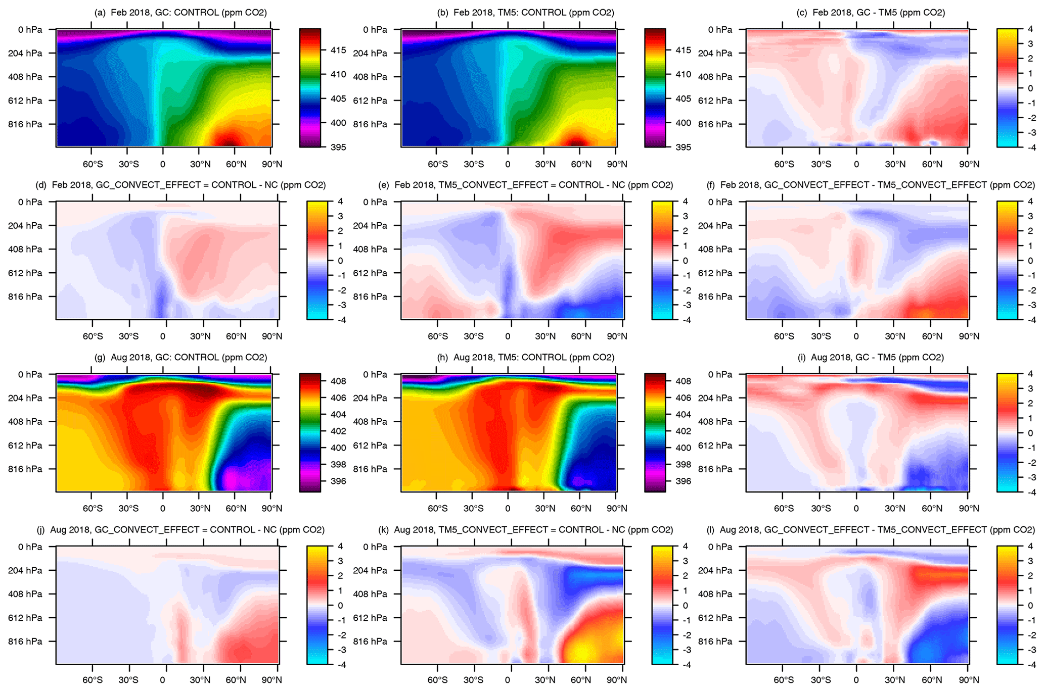
Figure 1 Vertical curtains of zonal-mean CO₂ dry-air mole fractions for February (top two rows) and August 2018 (bottom two rows). All quantities are monthly averages. The first and third rows (panels a–c and g–i, respectively) show model control simulations and differences, averaged zonally. The second and fourth rows (panels d–f and j–l, respectively) show the convective effect (control experiment minus the no-convection, NC, experiment) in each model and the GEOS-Chem minus TM5 difference between them. The first column represents GEOS-Chem simulations, the second column is TM5, and the third column is the GEOS-Chem minus TM5 difference.

2.3 Vertical mixing perturbation simulations

We ran three perturbation experiments on each transport model, with each simulation extending from 1 January 2016 to 31 December 2018. Control runs use the standard vertical transport in the models, unmodified from their stock configurations. The first experiment involved turning off convection in both CTMs. These will be called the “no-convection” or “NC” runs. The second experiment involved leaving convection on but turning off diffusive mixing in the models. These will be termed “no-diffusion” (“ND”) runs. It should be noted that vertical advection as part of the resolved wind fields in each model still remains in both perturbation and control runs for both models. We introduce the notion of a “convective effect”, which we are defining as control – NC – and a “diffusive effect” as control – ND. The diffusive and convective transport effects are not independent. The two processes have significant interactions such that total parameterized vertical transport is greater than the sum of the convective and diffusive effects. Exploring this nonlinear interaction, while intriguing, is beyond the scope of this paper. As a result, experiments in which both convection and diffusion are turned off will not be discussed.

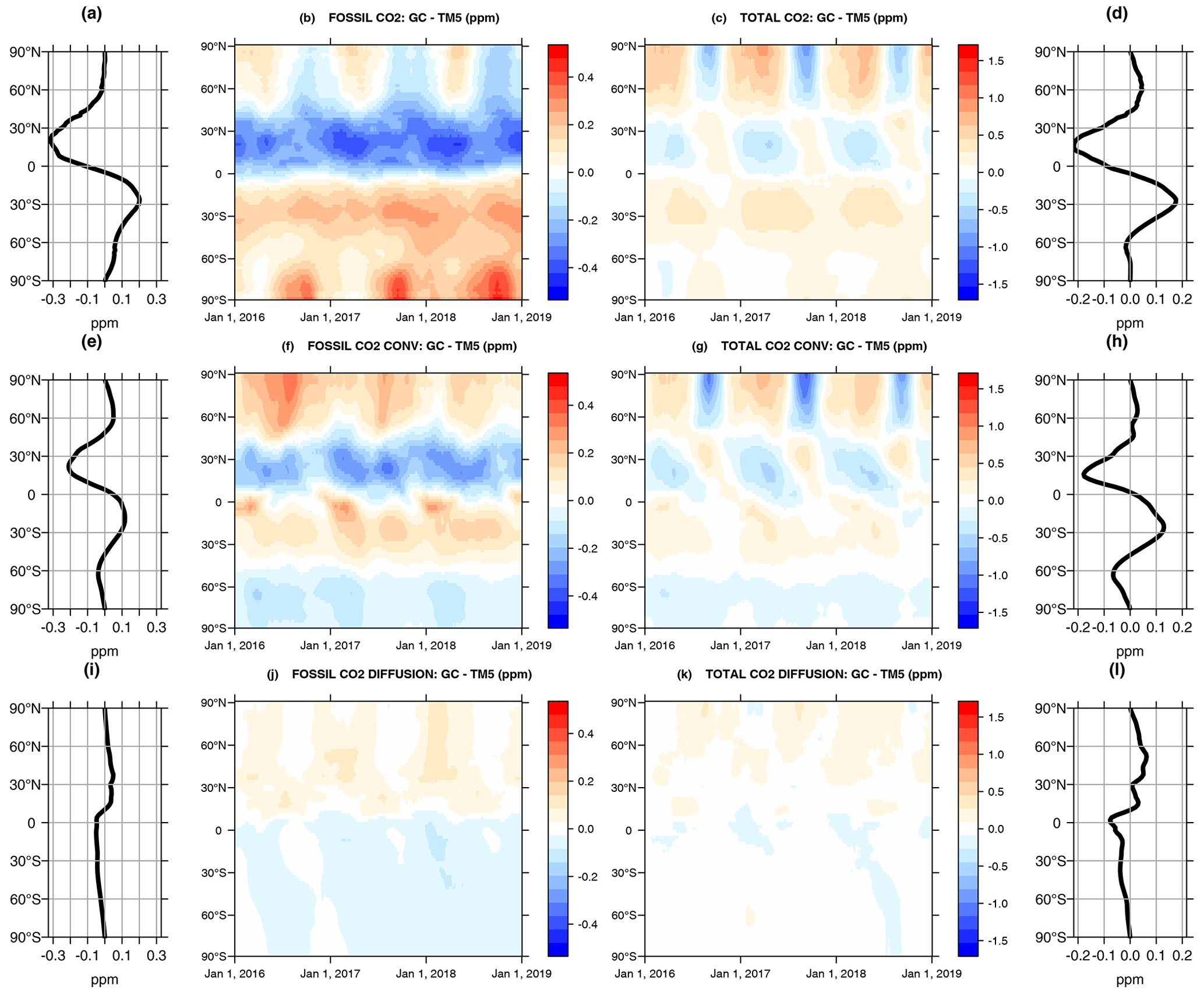
Figure 2 Zonally averaged pressure-weighted average CO₂ differences between GEOS-Chem and TM5, plotted as a function of latitude in side integrals and as a function of latitude and time in the central panels in the dry-air mole fraction. Column 1 represents the 3-year average of the second columns. Column 4 represents the 3-year average of the third columns. Note the differences in scale between the fossil and total CO₂ plots.

3 Results

In this section, we show the differences between the TM5 and GEOS-Chem control simulations and differences in the NC and ND cases from several perspectives. First, we show a zonally averaged vertical “curtain” by latitude which illustrates how the differences manifest themselves in the vertical. We then show two projections of the differences relevant to the major types of observational data used in flux inversions of CO₂. The first are time–latitude (Hovmöller) plots of zonal-mean column-average CO₂ (XCO₂), which is relevant to analysis of satellite CO₂ retrievals. The second are seasonal maps of differences in the planetary boundary layer at 400 m above ground level, meant to represent transport impacts on the ground-based in situ observational network.

3.1 Vertical curtains

Zonal-average “curtains” (latitude by vertical dimension) of CO₂ from the control and NC simulations in the two models are presented in Fig. 1. These curtains are shown for typical Northern Hemisphere winter (February) and summer (August) conditions. The expected buildup of CO₂ from fossil emissions and terrestrial biospheric respiration in boreal winter is evident at the northern midlatitudes to high latitudes in both models' control simulations (panels a and b). The overall differences between the GEOS-Chem and TM5 control runs are shown in panel c. The convective effects in the two models for February and the GEOS-Chem minus TM5 difference in convective effects are portrayed in the second row (panels d–f). The difference in convective effects (panels f and l) bears a remarkable similarity to the control simulation difference (panels c and i). This suggests visually that the GEOS-Chem minus TM5 difference in zonal-mean CO₂ is strongly driven by the convective effect. Indeed, the fields are strongly correlated (February: panels a and c, r=0.72, p<0.0001; August: panels d and f, r=0.83, p<0.0001). This will be further discussed in Sect. 4 below. The diffusive effect (not shown here) is about 3 times larger in magnitude but is strongly concentrated near the surface. The diffusive effects are shown in Figs. S2 and S3.

The last two rows of Fig. 1 show the same quantities as the first two but for Northern Hemisphere summer (August). Terrestrial biosphere uptake results in a deficit of CO₂ in the troposphere poleward of the northern midlatitudes. Again, the difference in the convective effect (panel l) is visually similar to the control simulation differences (panel i).

3.2 XCO₂ differences

Zonal averages of the GEOS-Chem minus TM5 difference in XCO₂ as a function of latitude and time are shown in the middle two columns of Fig. 2. Three-year averages of the differences are shown in the side panels and present a possible proxy or metric for the transport error effect on annual source/sink estimates of CO₂ from inversions. As in the previous vertical curtain plots, the convective effect differences shown in the middle row of Fig. 2 bear a strong resemblance to the total difference between the control runs shown in the top row of Fig. 2. Vertical diffusivity effects as a column average (bottom row of Fig. 2) are of a much smaller magnitude. It is also worth pointing out that, despite the strong seasonal patterns of differences seen in total CO₂ (Fig. 2c and g), the annual mean differences in total CO₂ (Fig. 2d and h) and fossil CO₂ (Fig. 2a and e) are quite similar and thus likely driven by differences arising from fossil fuels.

Figure 3 shows the 2016–2018 spatially resolved time mean XCO₂ difference between GEOS-Chem and TM5. This figure illustrates the zonal variability of the XCO₂ differences, which was not shown in Figs. 1 and 2. The large band of negative differences evidenced by the blue band at the lower northern latitudes is driven in large part by differences aloft shown in Fig. 1 and not by differences near the surface. There is an anomalously high difference over China, which is not due to a deviation of the difference pattern aloft but a combination of weaker mixing in GEOS-Chem and anomalously strong fossil-fuel emissions over eastern China. Reproducing Fig. 1c only over the area of enhancement in Fig. 3, approximately 105 to 120^∘ E longitude, results in PBL concentrations that are enhanced by 1–2 ppm CO₂ over the majority of the lower 20 %–25 % of the atmosphere and is the strongest contributor to the column-average results in the spatial anomaly seen in Fig. 3.

Seasonal summaries of the XCO₂ (Fig. 2) subsetted into 45^∘ latitude bands are shown in Fig. S4. There is excellent agreement between the differences in the convective effect and the differences in the control simulations, suggesting that convection differences between GEOS-Chem and TM5 are the predominant control on seasonal XCO₂ transport differences.

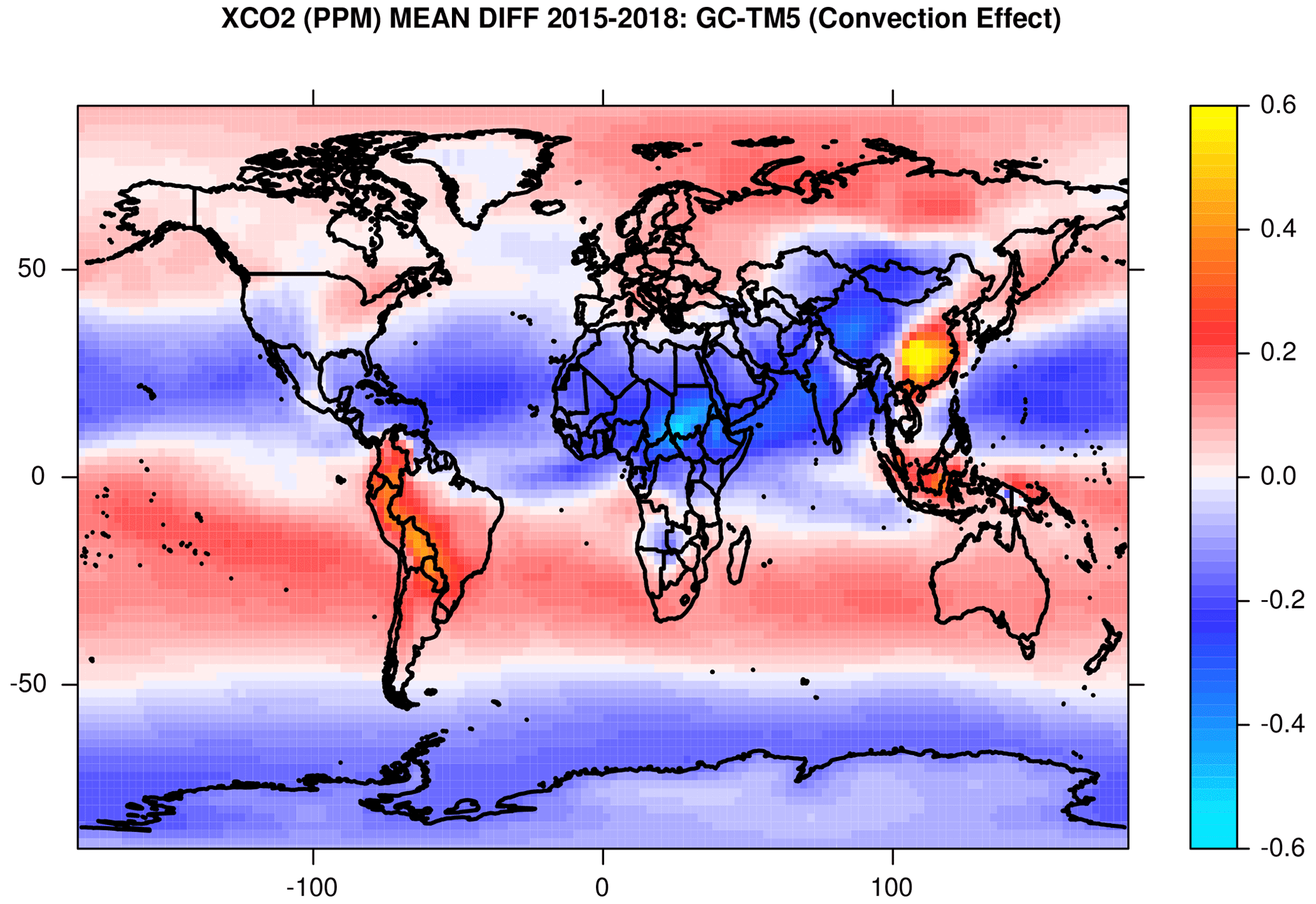
Figure 3 The 2016–2018 average XCO₂ difference between GEOS-Chem and TM5 “convective effects” (i.e., control – NC cases) using the total CO₂ tracer.

3.3 Impacts on near-surface CO₂

In the planetary boundary layer near intense surface sources and sinks of CO₂, the monthly average differences in the diffusive effect between the models are on the order of 10 ppm (Fig. 4). This is an order of magnitude larger than the model differences in the column seen in Fig. 2. There is a marked seasonality to the difference of the CO₂ mole fraction at this level (leftmost column, panels a, d, and g), and the convective and diffusive effect patterns in both seasons (topmost two rows, panels a–f) appear anti-correlated at large scales. We will return to discuss this in Sect. 4.

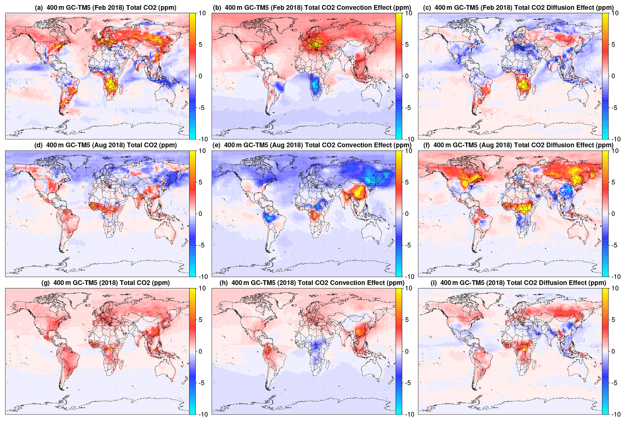
Figure 4 Monthly and annual average near-surface model CO₂ differences. Results have been interpolated to the 2^∘ × 2.5^∘ GEOS-Chem grid and 400 m height above ground level.

4 Discussion

4.1 Annual flux biases from convection uncertainty at zonal scales

Exploratory analysis of the location of long-term carbon sinks is commonly performed by considering large zonal bands in order to contrast the tropics, extratropics, and high latitudes (Stephens et al., 2007; Schimel et al., 2014), each of which has different mechanistic reasons to develop sources or sinks of carbon in a warming climate. The difference in the convection effect across CTMs, as seen in the right-hand column of Fig. 2, generates a significant first-order bias on these important annual zonal scales.

4.2 Remaining model XCO₂ differences after accounting for convection

An examination in Fig. 1c and f shows that while the convective effect difference largely explains the control simulation differences between the two models away from the surface, it does not extend to the same altitude as the control simulation differences. This remaining difference bears some similarity to the difference in ND runs (Figs. S2 and S3), indicating that while convection may be the main driver of the vertical differences in the model, it is likely that low-level PBL diffusivity differences also play a role.

4.3 Seasonal cycle of XCO₂

Agreement on the seasonal cycle of XCO₂ appears quite good between the GEOS-Chem and TM5 control runs, with the amplitude of the average zonal seasonal differences on the order of 1 ppm or less at 45^∘ N and poleward. GEOS-Chem minus TM5 differences in modeled seasonal cycles at TCCON locations are 10 %–15 % of the amplitudes reported by Lindqvist et al. (2015). While this difference is small, it is likely still significant to science hypotheses attempting to explain observed decadal-scale changes in seasonal amplitude (Graven et al., 2013). Accounting for differences in convection reduces that difference by another order of magnitude, resulting in great agreement in XCO₂ on seasonal-cycle amplitudes. Hence a focus on improving the modeling of convective mixing of trace gases could have a significant impact on the ability to constrain high-latitude seasonality.

4.4 Regional effects of convection uncertainty

The effect of uncertainty in the parameterized modeling of vertical mixing, and convection in particular, drives systematic differences in XCO₂. These concentration differences then manifest themselves as the first-order source of flux bias across large zonal bands amongst satellite CO₂-constrained flux-inversion models (Schuh et al., 2019). However, in some regions there are notable exceptions to the zonal mean of transport differences. One of these is over eastern Asia in the general area of China (Fig. 3). This anomaly to the zonal average largely arises from model differences in the spatially varying convection field (Taszarek et al., 2021) acting on large regional sources of CO₂ fossil-fuel consumption (Schuh et al., 2022). While total CO₂ is plotted in Fig. 3, one can see that the signal comes largely from the fossil-fuel-related portion of the CO₂ budget (cf. Figs. S5, S6, and S7). Similar patterns emerge across areas of critical biological importance, such as the Amazon and equatorial Africa (Fig. S7), and even emerge at the national scales there (Fig. S8). These could result in regional flux anomalies that are dependent on the particular CTM being used in a flux inversion.

4.5 Compensating effects of turbulent mixing and deep convection in the PBL

While parameterized diffusion and convection cause mixing in different parts of the column, they both act to move signals of surface exchange up, away from the PBL, and into the free troposphere. Historically, measurements of active and passive chemical species have been made more commonly within the PBL or at the surface than in the free troposphere. The availability of measurements near the surface without a correspondingly strong constraint on upper-atmospheric abundances means that those measurements speak strongly to the overall rate of ventilation of the PBL and not necessarily which process is responsible for the needed mixing. We speculate that CTMs may meet this constraint by using a different overall balance of convection and diffusion. The combination of remotely sensed total-column abundance with in situ measurements concentrated in the PBL may help to provide the needed constraint on vertical distribution to identify a correct balance of these mixing processes. In particular, this is an area where aircraft observations, campaign data (e.g., Atmospheric Tomography Mission (ATOM), ACT-America), and more operational data (e.g., In-Service Aircraft for a Global Observing System (IAGOS), NOAA light aircraft profiles) could provide a useful constraint.

4.6 Potential issues with direct comparison of GEOS-Chem and TM5 convection implementations

The parent models for GEOS-Chem and TM5 simulate convection differently. Some of the vertical movement associated with convection is explicitly resolved, depending on the model grid resolution. Non-resolved movement is parameterized using significantly different schemes. NASA's GEOS-5 MERRA2 reanalysis uses the relaxed Arakawa–Schubert convection scheme (Moorthi and Suarez, 1992), an updraft-only detraining plume cloud model (Molod et al., 2012), to provide driving convective mass fluxes used for GEOS-Chem. Version Cy31r2 of the IFS model was used to create the ERA-Interim reanalysis (Dee et al., 2011) used to drive the present TM5 simulations. The IFS uses the Tiedtke convection scheme (Tiedtke, 1989) to provide upward and downward plume entrainment and detrainment mass fluxes at each model level and as a means to represent shallow, intermediate, and deep convection. Both GEOS-Chem (Stanevich, 2018) and TM5 (based on the TM3 model from Heimann and Korner, 2003) interpret convective mass fluxes from their parent models to drive relatively simple mixing schemes. This mixing can be represented by a matrix specifying exchange among the layers in the column of a given grid cell.

While the RAS and Tiedtke convective parameterizations are different, we can still perform qualitative comparisons of the upward convective mass fluxes from the parent models under investigation here. While the downdraft component from TM5 is important, it is an order of magnitude weaker than the updraft component, as can be seen in Fig. S9. The comparison (Fig. S9) shows convective activity that is significantly different between the two models and highlights shallow convection features driving lower-tropospheric mixing in TM5 that do not appear in GEOS-Chem. This would appear to support past research highlighting differences between shallow convection features in MERRA and ERA-Interim (Posselt et al., 2012; Naud et al., 2014). This would suggest that the differences in CTM convective transport reported here result largely from differences in convection in the parent models as opposed to variations in how convective mixing is implemented in the CTMs. This confirms the findings of Folkins et al. (2006), Donner et al. (2007), and Orbe et al. (2017). Comparisons to long-lived trace gases like SF₆ might allow more definitive conclusions about how differences in parent-model convection and differences in their re-implementations in CTMs drive the large-scale differences seen in this paper (Denning et al., 1999a; Peters et al., 2004). Other metrics such as the stratospheric age of air (Krol et al., 2018) could provide insight into the differences seen here.

4.7 Looking forward

Recent analyses suggest that vertical transport in GEOS-Chem may be responsible for systematic biases in model performance against comparisons to CH₄ and SF₆ observations (Schuh et al., 2019; Stanevich et al., 2021). Part of this suspected vertical mixing issue may be due to imperfect reproduction of parent GEOS5 model transport (Yu et al., 2017). In preliminary analysis of meridional gradients of trace gases, the GEOS5 parent model does not appear to exhibit the same systematic biases as the GEOS-Chem CTM (personal communication: Brad Weir, NASA-GMAO). When using offline parent convective mass flux fields, in theory, convective mixing of trace gases via resolved vertical velocity should be damped with increased averaging in time and space and decreased horizontal model resolution (Yu et al., 2017). Furthermore, the coarse temporal nature, e.g., 3 h or more, of the convective mass-flux averaging leads to an information loss because the higher time-resolution covariance between tracer fields and vertical motion is lost. The resolved vertical velocity in 0.5^∘ by 0.667^∘ MERRA2 is similar in location and magnitude to that from the approximately 80 km ERA-Interim (Sourish Basu, NASA-GMAO, personal communication, 9 August 2022). This should not be surprising due to the similar horizontal resolutions of the model fields and suggests that the averaging of resolved vertical velocity fields to the coarser-resolution CTM grids is likely not the reason for the differences shown in this paper.

Ideally, one would desire a CTM's transport to asymptotically converge to the parent model's transport as model spatial and temporal resolution increases to the native resolution of the parent model, but this has not been demonstrated. It is worth noting that past work (Prather et al., 2008) utilizing two CTMs acting on the same parent meteorology has demonstrated the difficulty in characterizing this convergence. Tests are currently underway with high time- and space-resolution GEOS5 meteorology via the GEOS-Chem High Performance (Martin et al., 2022) model to gauge this convergence. These tests will help to determine whether results such as Yu et al. (2017) are sufficient to explain all deficiencies in CTM vertical transport.

It is also worth noting that despite the clear patterns of difference in the large-scale convective mass fluxes from parent models used as inputs into GEOS-Chem and TM5 (see Fig. S9), there are likely other factors at play which could cause differences in vertical transport. For its advection scheme, TM5 uses parent-model mass fluxes and a corresponding flux-form advection scheme, whereas GEOS-Chem explicitly uses interpolated parent-model winds to diagnose mass fluxes for advection. The use of winds to drive advection, as opposed to mass fluxes, has been shown to be a likely source of error and bias (Jöckel et al., 2001). As a result of this, tests are also currently underway using the GEOS-Chem High Performance (Martin et al., 2022) model to investigate the magnitude of this bias and to what degree those model errors and related errors in horizontal divergence might be related to vertical transport in GEOS-Chem (Sebastian Eastham, personal communication, 10 June 2022).

5 Conclusions

The systematic large-scale patterns in XCO₂ differences associated with transport first presented in Schuh et al. (2019) have been shown to result primarily from differences in the parameterization of convective mixing. This is the most important source of transport uncertainty for satellite-based flux-inversion studies and is on the same order as the expected biases in XCO₂ retrievals. We have shown that, for the simulation of concentrations near the surface, diffusive mixing in the PBL has a bigger effect than deep convection. It can therefore be expected that inversions based upon in situ measurements would be more sensitive to modeled vertical diffusion in the PBL than modeled deep convection.

The significance of uncertainty in simulated convection for model ensembles assimilating XCO₂, such as those of Crowell et al. (2019) and Peiro et al. (2022), warrants further exploration of model convective parameterizations. Convection alone drives 10 %–15 % differences in XCO₂ seasonality between the two models studied here and explains the vast majority of total model differences in simulated XCO₂ seasonality. We have also shown that convection drives the majority of the meridional difference in annual average XCO₂, a proxy for the meridional distribution of annual sources and sinks in the related flux-inversion models. Therefore, we feel that future efforts to characterize transport uncertainty and how it relates to flux-inversion results would benefit tremendously from a more thorough exploration of differences in parent-model convection.