Variations in global zonal wind from 18 to 100 km due to solar activity and the quasi-biennial oscillation and El Niño–Southern Oscillation during 2002–2019

Variations of global wind are important in changing the atmospheric structure and circulation, in coupling of atmospheric layers, and in influencing the wave propagations. Due to the difficulty of directly measuring zonal wind from the stratosphere to the lower thermosphere, we derived a global balance wind (BU) dataset from 50^∘ S to 50^∘ N and during 2002–2019 using the gradient wind theory and SABER temperatures and modified by meteor radar observations at the Equator. The dataset captures the main feature of global monthly mean zonal wind and can be used to study the variations (i.e., annual, semi-annual, ter-annual, and linear) of zonal wind and the responses of zonal wind to quasi-biennial oscillation (QBO), El Niño–Southern Oscillation (ENSO), and solar activity (F_10.7). The same procedure is performed on the MERRA-2 zonal wind (MerU) to validate BU and its responses below 70 km. The annual, semi-annual, and ter-annual oscillations of BU and MerU have similar amplitudes and phases. The semi-annual oscillation of BU has peaks around 80 km, which are stronger in the southern tropical region and coincide with previous satellite observations. As the increasing of the values representing QBO wind, both values of representing BU and MerU (short for BU and MerU) change from increasing to decreasing with the increasing height and extend from the Equator to higher latitudes. Both BU and MerU increase with the increasing of the values of multivariate ENSO index (MEI) and decrease with increasing F_10.7​​​​​​​ in the southern stratospheric polar jet region below 70 km. The responses of winds to ENSO and F_10.7 exhibit hemispheric asymmetry and are more significant in the southern polar jet region. While above 70 km, BU increases with the increasing of MEI and F_10.7. The negative linear changes of BU at 50^∘ N are absent in MerU during October–January. The discussions on the possible influences of the temporal intervals and sudden stratospheric warmings (SSWs) on the variations and responses of BU illustrate the following: (1) the seasonal variations and the responses to QBO are almost independent on the temporal intervals selected; (2) the responses to ENSO and F_10.7 are robust but slightly depend on the temporal intervals; (3) the linear changes of both BU and MerU depend strongly on the temporal intervals; (4) SSWs affect the magnitudes but do not affect the hemispheric asymmetry of the variations and responses of BU at least in the monthly mean sense. The variations and responses of global zonal wind to various factors are based on BU, which is derived from observations, and thus provide a good complement to model studies and ground-based observations.

1 Introduction

Atmospheric dynamics field (temperature, wind, etc.) and species not only exhibit latitude, longitude, and height variations, but also exhibit temporal variations with periods ranging from days, months to years, and even decades. The temporal variations can be ascribed into long-term variations, intra-annual and inter-annual variations. Here the long-term variations mean the linear term or linear change in a regression model and on a timescale longer than one solar cycle in the middle and upper atmosphere. The long-term variations of the middle and upper atmosphere have received attention due to greenhouse-gas-driven anthropogenic climate change and its influences on atmospheric drag and thus our space vehicles (Beig et al., 2003, 2008; Laštovička, 2017; Yue et al., 2019b; Mlynczak et al., 2022; Zhang et al., 2023). The intra-annual variations mainly include annual (AO), semi-annual (SAO), and ter-annual (TAO) oscillations. These variations are mainly cause by the revolution of earth with its oblique axis relative to the ecliptic plane. Their amplitudes depend on latitude and height (Dunkerton, 1982; Garcia et al., 1997; Randel et al., 2004; Smith et al., 2017).

The inter-annual variations are mainly caused by the coupling among different atmospheric layers, sea surface temperature, and solar activity, such as the following: the QBO (quasi-biennial oscillation) in the tropical regions has periods of 2–3 years due to wave–mean-flow interactions (Baldwin et al., 2001). The QBO signal can also be seen in the mesosphere, which is anti-phase to the stratospheric QBO due to the selective critical-layer filtering (Baldwin et al., 2001; Burrage et al., 1996; Xu et al., 2007). Recent studies have revealed that the mesospheric QBO is a seasonally locked phenomenon and occurs only in vernal equinox when the westward winds enhanced every 2 or 3 years and might be an ephemeral phenomenon (Venkateswara Rao et al., 2012; Kumar, 2021). The ENSO (El Niño–Southern Oscillation) is used to characterize the changes in sea surface pressure and temperature (Domeisen et al., 2019). It has been reported that the slight change of ENSO can affect global middle and upper atmosphere through the coupling of atmosphere and ocean and wave propagation (Baldwin and O'Sullivan, 1995; Randel et al., 2009; Li et al., 2013; Lin and Qian, 2019). The solar activity can be represented by its radiation flux at 10.7 cm (F_10.7); it can influence the atmosphere from upper to below through photon absorption and high-energy particle precipitation and ion deposition (Li et al., 2011; Beig et al., 2008; Qian et al., 2019; Venkat Ratnam et al., 2019). Moreover, the temporal variations may be coupled among different timescales: the coupling between SAO and QBO is mainly due to the selectively filtering and absorbing of equatorial waves and gravity waves by QBO winds (Li et al., 2012; Smith et al., 2017); the coupling between QBO and ENSO is mainly due to the stronger wave activity in the warm-phase ENSO (i.e., El Niño), which accelerates the downward propagation of QBO (Domeisen et al., 2019; Taguchi, 2010).

The variations and responses of temperature and trace gases (e.g., CO₂, H₂O) in the middle and upper atmosphere have been well studied through observations and model simulations (Emmert et al., 2012; Yue et al., 2015, 2019a; Laštovička, 2017; Lübken et al., 2008; Garcia et al., 2019; She et al., 2019; Yuan et al., 2019; Mlynczak et al., 2022). In contrast, the variations and responses of wind field are more complex than those of temperature due to the direct external forcings and the indirect dynamical coupling between waves and mean flow (Qian et al., 2019). In fact, wind field is an important atmospheric parameter since it is a direct driver of atmospheric circulation and influences the atmospheric structure. Moreover, wind field plays important roles in transporting mass and chemical species, in distributing and re-distributing momentum and energy, and in modulating the propagation and dissipation of atmospheric waves (i.e., gravity waves, tides, and planetary waves). This in turn affects the atmospheric circulation and structure indirectly. Thus, the variations and long-term variations of winds should also be studied.

Ground-based radar observations have revealed long-term variations of mean wind in the mesosphere and lower thermosphere (MLT) region at several stations. The medium-frequency (MF) radar observations at Tirunelveli (8.7^∘ N, 77.8^∘ E) from 1993 to 2006 showed that the monthly mean zonal wind was dominated by SAO with eastward peak during solstice and exhibited QBO signal with periods 2–3 years (Sridharan et al., 2007). Using the observations by four MF radars and three meteor radars in the latitudes from 21^∘ S to 22^∘ N during 1990–2010, Venkateswara Rao et al. (2012) showed that the zonal wind exhibited both negative and positive trends, whose magnitudes depended on stations and the temporal intervals of the observations. By combining the zonal wind at ∼ z = 70–80 km observed by rocketsondes, a satellite, and a mesosphere–stratosphere–troposphere (MST) radar over the Indian region (8.5 to 18.5^∘ N and 69 to 89^∘ E), Venkat Ratnam et al. (2013) constructed a long-term dataset from 1977 to 2010. They showed a decreasing trend of 2 m s⁻¹ yr⁻¹ (or 20 m s⁻¹ per decade) in February and March at 72.5 and 77.5 km (Fig. 2 of their paper). However, the trends are not significant from May to August. These observations coincided with the results simulated by the Thermosphere-Ionosphere-Mesosphere-Electrodynamics General Circulation Model (TIME-GCM) after doubling the CO₂ concentration (Venkat Ratnam et al., 2013). Recently, after extending the observation data to 2016, Venkat Ratnam et al. (2019) found a decreasing trend at ∼ z = 60–80 km and an increasing trend of 4–5 m s⁻¹ per decade at ∼ z = 80–90 km and below ∼ 60 km. Using the temperature and wind simulated by Whole Atmospheric Community Climate Model with eXtended thermosphere and ionosphere (WACCM-X) and the radar observations at Collm (51^∘ N, 13^∘ E) during 1980–2014, Qian et al. (2019) showed that the zonal wind trends and the solar effects were, respectively, an order of ∼ ±5 m s⁻¹ per decade and ∼ ±5 m s⁻¹ per 100 SFU (1 SFU = 10⁻²² W m⁻² Hz⁻¹) but with large standard deviations. Using the historical simulations by WACCM6 during 1850–2014 (165 years), Ramesh et al. (2020) showed the responses of the temperature and zonal wind to QBO, ENSO, solar activity, ozone-depleting substance, carbon dioxide, and aerosol from the stratosphere to the lower thermosphere. They showed that the influences of solar activity are mainly in the mesosphere, while the influences of QBO and ENSO are mainly in the stratosphere and mesosphere. Moreover, these influences depend on latitudes.

The above observations and modeling studies revealed seasonal variations of zonal winds and their responses to QBO, ENSO, and solar activity in the mesosphere. However, the reported long-term (or linear) changes of zonal winds depended on specific locations and the temporal intervals of the data. At present, it is still a challenge to directly measure the atmospheric wind field from the stratosphere to the lower thermosphere. It is compelling to develop a wind dataset to represent the main features of global zonal winds and their temporal variations.

Recently, we developed a dataset of global monthly zonal mean zonal wind (short for BU) based on the gradient balance wind theory (Randel, 1987; Fleming et al., 1990; Xu et al., 2009a; Smith et al., 2017) and the temperature and pressure profiles measured by the Sounding of the Atmosphere using Broadband Emission Radiometry (SABER) instrument (Russell et al., 1999). To overcome the tidal alias above 80 km over the Equator (Hitchman and Leovy, 1985, 1986; Xu et al., 2009b; Smith et al., 2017), we replaced the BU with the zonal wind observed by a meteor radar at Koto Tabang (0.2^∘ S, 100.3^∘ E) (Hayashi et al., 2013; Matsumoto et al., 2016). The BU covers a latitude range of 50^∘ S–50^∘ N with steps of 2.5^∘ and height range of 18–100 km with steps of 1 km and a temporal range of 2002–2019. The BU coincides generally with re-analysis data, empirical wind models, observations by meteor radars and lidar (Liu et al., 2021a), and with the balance wind derived by Smith et al. (2017) above the Equator region. Thus, we focus on variations and responses of global zonal winds to various factors since the BU is a reasonable candidate for monthly mean zonal wind.

The solar activity effects on zonal winds in the MLT region are still unclear (Venkateswara Rao et al., 2012; Qian et al., 2019). It should be noted that the linear changes and solar activity have influences on the other signals (i.e., QBO, ENSO); one must isolate the contributions of different signals to get a clearer picture of the variations and responses of zonal winds. The long temporal (18-year) and entire height (18–100 km) intervals of BU are suitable to study the variations of zonal winds and their responses to QBO, ENSO, and solar activity. To separate the relative contributions of the variations and effects of QBO, ENSO, and solar activity on zonal winds, the multiple linear regression (MLR) method will be used.

To evaluate the reliability of BU and the corresponding responses below 70 km further, we will perform the same MLR on the zonal wind of Modern-Era Retrospective analysis for Research and Applications, version 2 (MERRA-2). The BU will provide the unique wind results at 70–100 km. MERRA-2 provides assimilated meteorological field from surface to ∼ 75 km (72 levels). It has temporal, longitude, and latitude intervals of 3 h, 0.625^∘, and 0.5^∘, respectively (Molod et al., 2015; Gelaro et al., 2017). Each MERRA-2 zonal wind profile is interpolated to uniform vertical grid with a step of 1 km. Then the monthly zonal mean wind (MerU) is calculated by averaging these profiles in a latitude band of 5^∘ with an overlap of 2.5^∘ in each month. The variations of MerU and their responses to QBO, ENSO, and solar activity are used to compare with those of BU below 70 km. MERRA-2 is used here due to its good consistency with other datasets, such as the consistency of the monthly mean zonal winds between MERRA-2 and the QBO wind in Singapore (Coy et al., 2016) and the consistency of the changes in subtropical and polar jets between MERRA-2 and other re-analyses (e.g., MERRA, ERA-Interim, JRA-55, and NCEP CFSR) (Manney and Hegglin, 2018).

2 Data and multiple linear regression

2.1 BU data and reference time series

The detailed description and validation of BU can be found in Liu et al. (2021a). Here, we provide a short summary of this dataset. The BU dataset includes the monthly mean zonal wind in the height range of 18–100 km with step of 1 km and at latitudes of 50^∘ S–50^∘ N with a step of 2.5^∘ from 2002 to 2019. BU is mainly derived from the temperature and pressure observations by the SABER instrument (Russell et al., 1999) and based on the gradient wind theory (Fleming et al., 1990; Randel, 1987; Xu et al., 2009a; Smith et al., 2017):

$$\begin{array}{}\text{(1)}& {\displaystyle \frac{{\stackrel{\mathrm{‾}}{u}}^{\mathrm{2}}}{a}}\tan \mathit{\phi }+f\stackrel{\mathrm{‾}}{u}=-{\displaystyle \frac{\mathrm{1}}{a\stackrel{\mathrm{‾}}{\mathit{\rho }}}}{\displaystyle \frac{\partial \stackrel{\mathrm{‾}}{p}}{\partial \mathit{\phi }}}.\end{array}$$

Here, f=2Ωsin φ is the Coriolis factor, $\mathrm{\Omega }=\mathrm{2}\mathit{\pi }/\left(\mathrm{24}\times \mathrm{60}\times \mathrm{60}\right)$ is the earth rotation frequency (unit of rad s⁻¹), a is the radius of the earth. $\stackrel{\mathrm{‾}}{u}$ and $\stackrel{\mathrm{‾}}{\mathit{\rho }}=\stackrel{\mathrm{‾}}{p}/R\stackrel{\mathrm{‾}}{T}$ are the BU and zonal mean density, respectively. R is the gas constant for dry air. At the Equator and above 80 km, the tidal alias on gradient wind is replaced by the monthly mean zonal wind measured by a meteor radar at 0.2^∘ S (Hayashi et al., 2013; Matsumoto et al., 2016). Equation (1) is used to calculate the BU in the latitude ranges of 10–50^∘ N and 10–50^∘ S. Above the Equator, the BU is calculated as $\stackrel{\mathrm{‾}}{u}=-({\partial }^{\mathrm{2}}\stackrel{\mathrm{‾}}{p}/\partial {\mathit{\phi }}^{\mathrm{2}})/\left(\mathrm{2}\mathrm{\Omega }a\stackrel{\mathrm{‾}}{\mathit{\rho }}\right)$ (Fleming et al., 1990; Swinbank and Ortland, 2003). At 2.5–7.5^∘ N and 2.5–7.5^∘ S, the BU is estimated by a cubic spline interpolation of the BU at 10–50^∘ N, 10–50^∘ S, and the reconstructed BU at the Equator. The detailed description can be found in Liu et al. (2021a).

For the consistency of BU and the monthly averaged zonal wind observed at a single station, Fig. 3 of Smith et al. (2017) showed that the monthly zonal wind from a meteor radar at Ascension Island (8^∘ S) coincides well with the BU at 81 and 84 km. This indicates that the monthly averaged zonal wind at a single station can represent the zonal average at least below 84 km. While above 84 km, Fig. 2a of Liu et al. (2021a) shows that the theoretical balance winds are mainly eastward. In contrast, the reconstructed winds (Fig. 2b and c of Liu et al., 2021a) from a meteor radar observation at Koto Tabang (0.2^∘ S) are mainly westward. The differences between the theoretical balance wind and meteor radar observations are mainly due to the tidal aliasing above 84 km (Hitchman and Leovy, 1985, 1986; Xu et al., 2009b; Smith et al., 2017). The comparisons between BU and other data (MERRA-2, HWM14 empirical model, meteor radar and lidar observations at seven stations from around 50^∘ N to 29.7^∘ S) illustrate good agreement. The good agreement suggests that BU is a reasonable candidate for monthly mean zonal wind. The large vertical extent and the 18-year internally consistent time series of BU make it is suitable to study the variations and responses to solar activity, QBO, and ENSO.

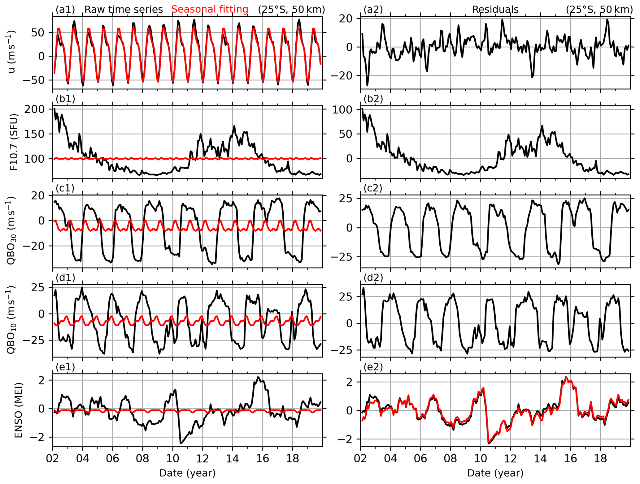
Figure 1 Example of BU and the reference time series (left column) and their de-seasonalized results (right column). The first row: BU at 25^∘ S and 50 km (black line in a1) and its seasonal fitting result (red line in a1), and the de-seasonalized BU (black line in a2). The second, third, and fourth rows: same captions as the first row but for solar activity (indicated by F_10.7), QBO at 30 hPa (QBO₃₀ or QBOA) and 10 at hPa (QBO₁₀ or QBOB), and ENSO (indicated by MEI index). The red line in (e2) is the residual of MEI index after removing the response of MEI to F_10.7.

The reference time series of solar activity, QBO, and ENSO are used to explore their possible influences on global zonal wind. The solar activity is represented by the solar radio flux at 10.7 cm in a 100 MHz band (F_10.7, Fig. 1b1; Tapping, 2013). The QBO is represented by the zonal wind at 30 hPa (∼ 25 km) and 10 hPa (30 km) (referred to as QBOA and QBOB in Fig. 1c1 and d1, respectively) over Singapore (1^∘ N, 104^∘ E) (Baldwin et al., 2001). Due to the propagation nature of QBO with height, we use the QBO winds at two different heights to represent the phase information of QBO. ENSO is represented by the multivariate ENSO index (MEI, Fig. 1e1; Zhang et al., 2019; Wolter and Timlin, 2011). These reference time series play important roles in studying the atmospheric coupling and have been widely used to study their influences on temperature, gravity waves, ozone, and carbon dioxide in the stratosphere and mesosphere (Randel and Cobb, 1994; Li et al., 2011; Yue et al., 2015; Liu et al., 2017; Randel et al., 2017).

2.2 Multiple linear regression

The detailed applications of MLR to retrieve the seasonal variations of winds and the responses of winds to F_10.7, QBOA, QBOB, and MEI can be ascribed to the following three steps. For illustrative purposes, the BU at 25^∘ S and 50 km (black in Fig. 1a1) is taken as an example to show the procedure of MLR. This procedure is also applied to winds at other latitudes and heights, but it results in different regression coefficients due to the latitudinal and height dependencies of the seasonal variations and the responses of winds to F_10.7, QBOA, QBOB, and MEI. We note that the wind direction is represented by its sign; i.e., the eastward (westward) wind is represented by positive (negative) value. Then the strength of wind is represented by its magnitude (or absolute value); i.e., stronger eastward (westward) wind has larger positive (negative) value. In the following, we use values (with sign and magnitude) to represent wind speeds. For example, the “increasing of BU” means the increasing of the values of BU. In a same way, the MEI index is also represented by its value.

First, we de-seasonalize the wind and reference time series by fitting the following harmonics through the least squares method. At each latitude and height, the wind series is fitted as

$$\begin{array}{}\text{(2)}& u\left(t_i\right)=u_{\mathrm{0}}+{\sum }_{k=\mathrm{1}}^{\mathrm{3}}{A}_k\cos \left[k\mathit{\omega }\left(t_i-{\mathit{\phi }}_k\right)\right]+u_{\mathrm{res}}\left(t_i\right).\end{array}$$

Here, t_i (i=1, 2, …, N) is the month number since February 2002. u₀ is the mean wind over the entire temporal interval, and u_res is the de-seasonalized wind. $\mathit{\omega }=\mathrm{2}\mathit{\pi }/\mathrm{12}$ (month), A_k, and φ_k are the amplitude and phase of the annual (AO, k=1), semi-annual (SAO, k=2), and ter-annual (TAO, k=3) oscillations, respectively. In the same way, Eq. (2) is used to de-seasonalize the reference time series of F_10.7, QBOA, QBOB, and MEI (shown in the left column of Fig. 1), and thus their de-seasonalized results (F10.7_res, QBOA_res, QBOB_res, MEI_res, shown in the right column of Fig. 1) can be obtained and will be used as predictor variables (or explanation variables).

The rationality or goodness of the seasonal fitting result is quantified by the R² score, which is the variations of the raw data explained by the model and defined as follows:

$$\begin{array}{}\text{(3)}& \begin{array}{rl}& R^{\mathrm{2}}=\mathrm{1}-\left\{{\sum }_{i=\mathrm{1}}^N{u}_{\mathrm{res}}^{\mathrm{2}}\left(t_i\right)/{\sum }_{i=\mathrm{1}}^N{\left[u\left(t_i\right)-\stackrel{\mathrm{‾}}{u}\right]}^{\mathrm{2}}\right\},\\ & \stackrel{\mathrm{‾}}{u}={\displaystyle \frac{\mathrm{1}}{N}}{\sum }_{i=\mathrm{1}}^{N}u\left(t_i\right).\end{array}\end{array}$$

The best fitting results in R²=1, which means that the fitting result is the same as the raw data. For example, the seasonal fitting of BU at 25^∘ S and 50 km is shown as a red line in Fig. 1a1. It coincides well with the raw BU series (black line in Fig. 1a1) with R²=0.967. This means that Eq. (2) explains 96.7 % of the variations of BU at 25^∘ S and 50 km. Moreover, for this case, the fitting result shows that the AO has an amplitude of 53.9 m s⁻¹ and is in the dominant position. Then the SAO has a smaller amplitude of 13.2 m s⁻¹, while the TAO is the weakest and has a amplitude of 3.9 m s⁻¹. The rationality of the fitting results (R²) at other latitudes and heights will be shown in Sect. 3.1.

Table 1 The correlation coefficients and their p values of regressors.

Second, we check the multicollinearity among the predictor variables, which are the de-seasonalized F_10.7, QBO₃₀, QBO₁₀, and MEI. The multicollinearity often leads to meaningless results if the correlation coefficients (CCs) between two or more predictor variables are significant. Here we calculate the CC and p value of each pair of predictor variables (Table 1). If the p value of a pair is less than 0.1 (or 0.05), one can state that the CC of this pair differs from zero at a confidence level of 90 % (or 95 %). And, thus, the multicollinearity of this pair is significant. In contrast, larger p values indicate lower confidence level and insignificant multicollinearity. Table 1 shows that the CCs of most pairs are less than 0.1, and their p values are larger than 0.1. This indicates that the multicollinearities of these predictor variables are insignificant and are approximately independent. On exception is the pair of F_10.7 and ENSO, which has a CC of 0.2022 with a p value of 0.0030. This indicates that the multicollinearity of F_10.7 and ENSO is significant at confidence level of 95 %. To improve the independency between F_10.7 and ENSO, a linear regression is performed with response variable of MEI index and predictor variable of F_10.7. The residual of MEI index, which excludes the influences of F_10.7, is used as a predictor variable to represent the effects of ENSO in the following MLR model. We note that the residual of MEI index is still noted as MEI_res in the following text. Now, the multicollinearity among the four predictor variables can be neglected and ensures a meaningful result of MLR in the next step.

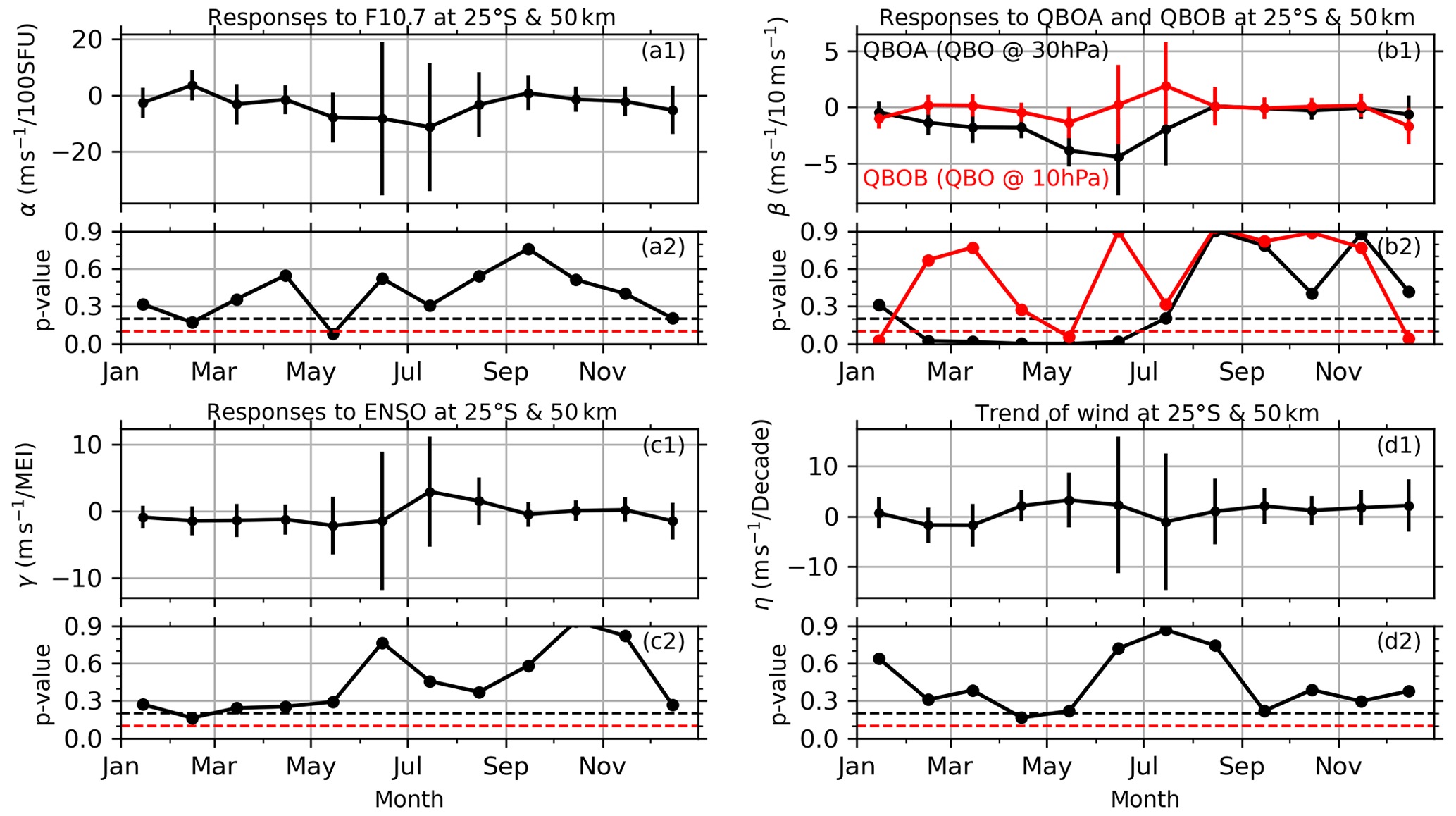
Figure 2 The monthly responses of BU at 25^∘ S and 50 km to solar activity (a), QBO (b), ENSO (c), and the linear variations of BU (d), as well as their p values. The error bars are the confidence interval at 90 % confidence level. The red and black dashed lines shown in the lower panel of each subplot indicate the p values of 0.05 and 0.1, respectively.

Third, MLR is applied to get the responses of winds (i.e., u_res in Eq. 1) to the four predictor variables (F10.7_res, QBOA_res, QBOB_res, MEI_res) prepared in the second step. In the MLR model, the response variable is the de-seasonalized wind (i.e., u_res in Eq. 1) at each latitude and height. The MLR model is written as

$$\begin{array}{}\text{(4)}& \begin{array}{rl}{u}_{\mathrm{res}}\left(t_i\right)& =\mathit{\alpha }F{\mathrm{10.7}}_{\mathrm{res}}\left(t_i\right)+{\mathit{\beta }}_{\mathrm{A}}{\mathrm{QBOA}}_{\mathrm{res}}\left(t_i\right)\\ & +{\mathit{\beta }}_{\mathrm{B}}{\mathrm{QBOB}}_{\mathrm{res}}\left(t_i\right)+\mathit{\gamma }{\mathrm{MEI}}_{\mathrm{res}}\left(t_i\right)+\mathit{\eta }{t}_i+\mathit{\epsilon }\left(t_i\right).\end{array}\end{array}$$

The regression coefficients α, β_A, β_B, and γ indicate the responses of wind to F_10.7, QBOA, QBOB, and MEI, respectively. The regression coefficient η is the linear variations or long-term trend. ε(t_i) is the residual of the fitting and can be used to estimate the standard deviation and p value of each coefficient with the help of variance–covariance matrix and the Student t test (Kutner et al., 2004; Mitchell et al., 2015). The monthly responses are obtained by selecting t_i in Eq. (4) only in that month of each of year. For example, the response in January can be obtained by selecting the date only in January of each year. The annual responses are obtained by using all the data during 2002–2019. Figure 2 shows the monthly responses of BU at 25^∘ S and 50 km to solar activity (a), QBO (b), ENSO (c), and the linear variations of BU (d), as well as their p values. The error bars are the confidence interval at 90 %. The responses of BU at 25^∘ S and 50 km to solar activity (Fig. 2a1) have an annual mean of −3.2 m s⁻¹ per 100 SFU with a p value of 0.05, which are mainly contributed from May–August, in which the negative peaks reach a value of −10 m s⁻¹ per 100 SFU in June and July but with larger p values (Fig. 2a2). In January–April and September–October, the responses of BU at 25^∘ S and 50 km to solar activity are very weak. This indicates that the responses of BU at 25^∘ S and 50 km to solar activity are stronger in the boreal summer and weaker in other months but have larger p values. The responses of BU at 25^∘ S and 50 km to QBO₃₀ and QBO₁₀ (Fig. 2b1) have annual means of −1.2 m s⁻¹/10 m s⁻¹ (p value ≈ 0.0) and −0.3 m s⁻¹/10 m s⁻¹ (p value = 0.22). The monthly responses of BU at 25^∘ S and 50 km to QBO₃₀ have negative peaks of ∼ 3–5 m s⁻¹/10 m s⁻¹ (p value < 0.1) in April–July, when QBO₃₀ reaches its eastward or westward peaks. Thus, the responses of BU at 25^∘ S and 50 km to QBO₃₀ are strong in the boreal summer. However, the monthly responses of BU at 25^∘ S and 50 km to QBO₁₀ are much weaker than those to QBO₃₀. The responses of BU at 25^∘ S and 50 km to ENSO (Fig. 2c1) have an annual mean of −0.31 m s⁻¹/MEI (p value = 0.56). The monthly responses of BU at 25^∘ S and 50 km to ENSO have negative peak in May and positive peaks in July and August but have large p values in May–November. The annual mean linear variations (Fig. 1h) is of 0.99 m s⁻¹ per decade (p value = 0.27). The monthly linear variations of BU at 25^∘ S and 50 km reach a peak of 3 m s⁻¹ per decade (p value < 0.2) in May. We note that the linear variation depends highly on the temporal span of the data and will be discussed in Sect. 4.1.

3 Seasonal variations and regression results

3.1 Seasonal variations

Figure 3 shows the amplitudes and phases of the seasonal variations of BU (upper row) and MerU (lower row). The R² scores (the fourth column) of both BU and MerU are larger than 0.8 at latitudes higher than 20^∘ N/S and below 85 km. This indicates that the variations of BU and MerU can be explained well by Eq. (2) and mainly contributed by the seasonal variations. However, above 85 km and in the tropical regions, the R² scores of BU are less than 0.6. This indicates that the variabilities of BU are influenced by some other factors, which were not included in Eq. (2). These factors might include (1) the phase change (eastward peak shifting from winter to summer) of zonal wind caused by the strong gravity wave dissipation at high latitudes (Liu et al., 2022), (2) the strong tides and short-term variabilities of zonal wind in the equatorial lower thermosphere (Xu et al., 2009b; Smith et al., 2017), (3) the imperfect BU in the extra-tropical lower thermosphere (Liu et al., 2021a), and (4) the strong QBO signals, which were not included in Eq. (2).

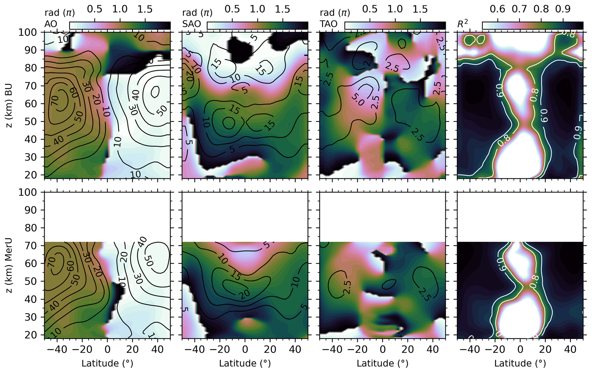
Figure 3 The latitude–height distributions of the amplitudes (contour lines) and phases (color scale) of seasonal variations and the R² scores (from left to right) of BU (upper row) and MerU (lower row).

The latitude–height distributions of the amplitudes and phases of AOs of BU and MerU exhibit general consistencies and slight discrepancy. The consistencies include the following: (1) both BU and MerU have peaks around 55 km in July in the Southern Hemisphere (SH) and around 65 km in January in the Northern Hemisphere (NH); (2) both BU and MerU have small amplitude below ∼ 30 km at all latitudes and throughout the height range in the tropical regions. The discrepancy is that the AO of MerU has larger amplitudes in the SH but smaller amplitudes in the NH than those of BU. The possible reason for the weaker AO of MerU in the NH is that it has a peak around 65 km, which might be caused by the damping layers of MERRA-2 and reduced the zonal wind (Ern et al., 2021). Above 80 km, the amplitude of AO is small. This is because the magnitudes of zonal wind above 80 km are less than those at around 60 km, where the stratospheric polar jet occurs.

The SAOs of both BU and MerU have nearly identical phases in the regions where their amplitudes are prominent. The amplitudes of the SAOs of both BU and MerU exhibit hemispheric asymmetry. At latitudes higher than 35^∘ S, the SAOs of both BU and MerU have peaks at ∼ z = 35–55 km. However, above 65 km, the SAO of BU is stronger than that of MerU. In the tropical regions, the SAOs of both BU and MerU are stronger in the SH than those in the NH. This coincides with the balance wind derived by Nimbus-7 Stratospheric and Mesospheric Sounder (Delisi and Dunkerton, 1988), the measurements by High Resolution Doppler Imager (HRDI) measurements, the assimilated data by UK Meteorological Office (UKMO) (Ray et al., 1998), and the balance wind derived from SABER and Microwave Limb Sounder (MLS) observations (Smith et al., 2017). Large discrepancies occur at latitudes higher than 40^∘ N, where the SAO of MerU is much stronger than that of BU below ∼ 70 km. Above 70 km, the SAO of BU reproduces the same pattern as that at around 40 km but has larger magnitudes and anti-phase.

The TAOs of both BU and MerU have same phases and peaks at ∼ z = 30–60 km and at latitudes higher than 25^∘ S. In the tropical regions and around 45 km, the TAO of BU has two peaks, which are approximately symmetric to the Equator, but the TAO of MerU has one peak over the Equator. At ∼ z = 50–70 km, the TAO of BU has larger amplitude than that of MerU. Above 80 km, the TAO of BU is asymmetric to the Equator and has a larger peak in the SH tropical region.

A short summary is that AO, SAO, and TAO of both BU and MerU have nearly identical phases in the regions where their amplitudes are prominent. Their consistencies are better in the SH than in the NH on the aspects of both patterns and magnitudes. The discrepancies of these seasonal variations are mainly in the NH. Above 70 km, the weak AO is due to the weaker wind as compared to that in the stratospheric jet region. The SAOs of BU around 50 and 80 km are hemispheric asymmetric and stronger in the SH, which coincides with the HRDI observations (Ray et al., 1998) and the balance winds derived from temperature observations by satellites (Delisi and Dunkerton, 1988; Smith et al., 2017). The TAO of BU above 80 km is hemispheric asymmetric and stronger in the SH.

3.2 Responses to solar activity

The latitude–height distributions of the responses of BU and MerU to F_10.7 (upper two rows of Fig. 4) exhibit general consistencies in July and October and in the annual mean. These consistencies include the following: (1) the negative responses at ∼ 30^∘ S and from 20 to 60 km in July, (2) the negative response around the Equator and ∼ 40 km in October, and (3) the negative response in the SH stratospheric jet region in the annual mean. In contrast, the discrepancies are the following: (1) stronger negative response (but insignificant) of BU in January at 50^∘ N, as compared to that of MerU, and (2) the positive responses of BU in July around 70 km and 20^∘ N/S, and in October around 65 km and above the Equator, which cannot be seen in MerU. The annual mean responses of BU and MerU are the following: (1) mainly negative in the regions extending from ∼ 30^∘ S/N to higher latitudes below ∼ 60 km and (2) mainly negative in the tropical regions and around ∼ 40 km. Above ∼ 80 km, the response of BU to F_10.7 is insignificant. The annual mean responses of BU to F_10.7 are mainly positive at 60–80 km. This feature has a similar pattern but larger amplitude as compared to the results simulated by WACCM-X (Ramesh et al., 2020).

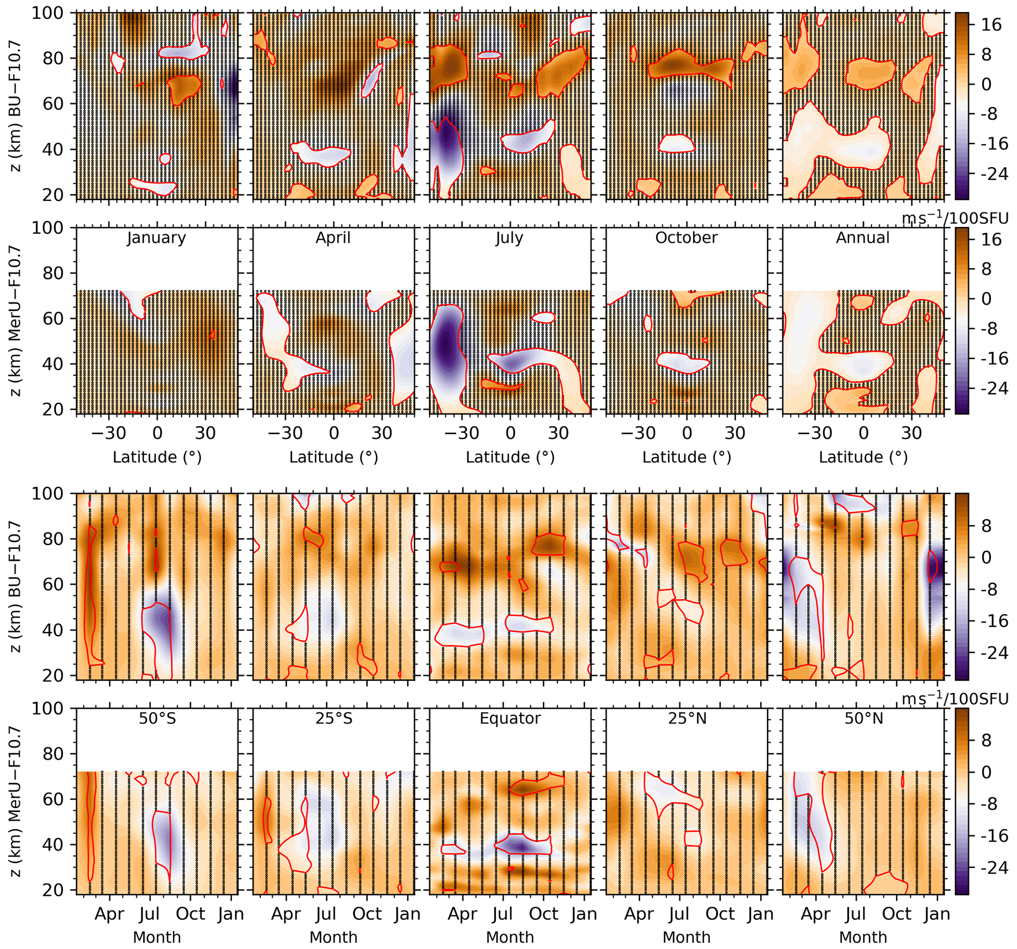
Figure 4 Upper two rows: latitude–height distributions of the regression coefficients of BU (the first row) and MerU (the second row) to F_10.7 in January, April, July, October, and annual mean (from left to right). Lower two rows: monthly-height (lower two rows) distributions of the regression coefficients of BU (the third row) and MerU (the fourth row) to F_10.7 at 50^∘ S–50^∘ N with interval of 25^∘ (from left to right). The black dots indicate that the regression coefficients with p values larger than 0.2. The red lines indicate the regression coefficients with p values of 0.1.

The monthly-height distributions of the responses of BU and MerU to F_10.7 (lower two rows of Fig. 4) exhibit general consistencies below ∼ 70 km. However, the discrepancies should be clarified, such as the stronger negative responses of BU in winter months (June–August at 50^∘ S and December–January at 50^∘ N) and the weaker negative responses of BU at ∼ 40 km over the equatorial as compared to those of MerU. It should be noted that the negative responses of winds at the southern and northern high latitudes can also be seen in the results simulated by WACCM-X (Ramesh et al., 2020).

The MF radar observations at Langfang (39.4^∘ N, 116.7^∘ E) revealed a positive correlation between zonal wind and solar activity from 2009 to 2020 during spring and summer at 80–84 km (Cai et al., 2021). However, another MF radar observations at Juliusruh (54.6^∘ N, 13.4^∘ E) revealed that the correlations between zonal wind and solar activity from 1990 and 2005 were positive during winter but negative in summer (Keuer et al., 2007). Our results coincide with the observations at Langfang but different from those at Juliusruh. The simulation study by Qian et al. (2019) showed that the solar activity effects on global zonal wind are sporadic in latitude and height distributions. They suggested that the zonal wind might be influenced by both the direct effects of solar radiance and the indirect effects of dynamic process such as wave–mean-flow interaction. Another possible mechanism is that the modulation of solar heating is in the ozone layer, which influences the meridional gradient of temperature and thus the zonal wind. However, this mechanism should be validated through observations or simulations. Qian et al. (2019) also proposed that the temporal intervals of data should be specified when we study the trends and solar activity effects since the trend drivers are different in different periods. This will be discussed in Sect. 4.1.

A short summary is that the annual mean responses of both BU and MerU to F_10.7 are more negative in the stratospheric polar jet region of SH than those of NH. Above the stratospheric polar jet, the responses of BU change from negative to positive with the increasing height. Around ∼ 80 km, the annual responses of BU to F_10.7 are mainly positive in the tropical region and in the high latitudes.

3.3 Responses to QBO

The latitude–height distributions of the responses of BU and MerU to QBO₃₀ (upper two rows of Fig. 5) exhibit general consistencies in all months and in the annual mean below ∼ 50 km. Such as the responses of BU and MerU to QBO₃₀ change from positive below 30 km to negative at ∼ z = 30–50 km and 25^∘ S–25^∘ N. The varying responses with height are mainly due to the downward propagation of QBO phase with time. This can be confirmed by the responses of BU and MerU to QBO₁₀ at a higher height (lower two rows of Fig. 5), where the responses of BU and MerU to QBO₁₀ change from negative to positive and then negative again. The discrepancy is that the responses of BU to QBO₃₀ and QBO₁₀ are slightly weaker than those of MerU below ∼ 50 km.

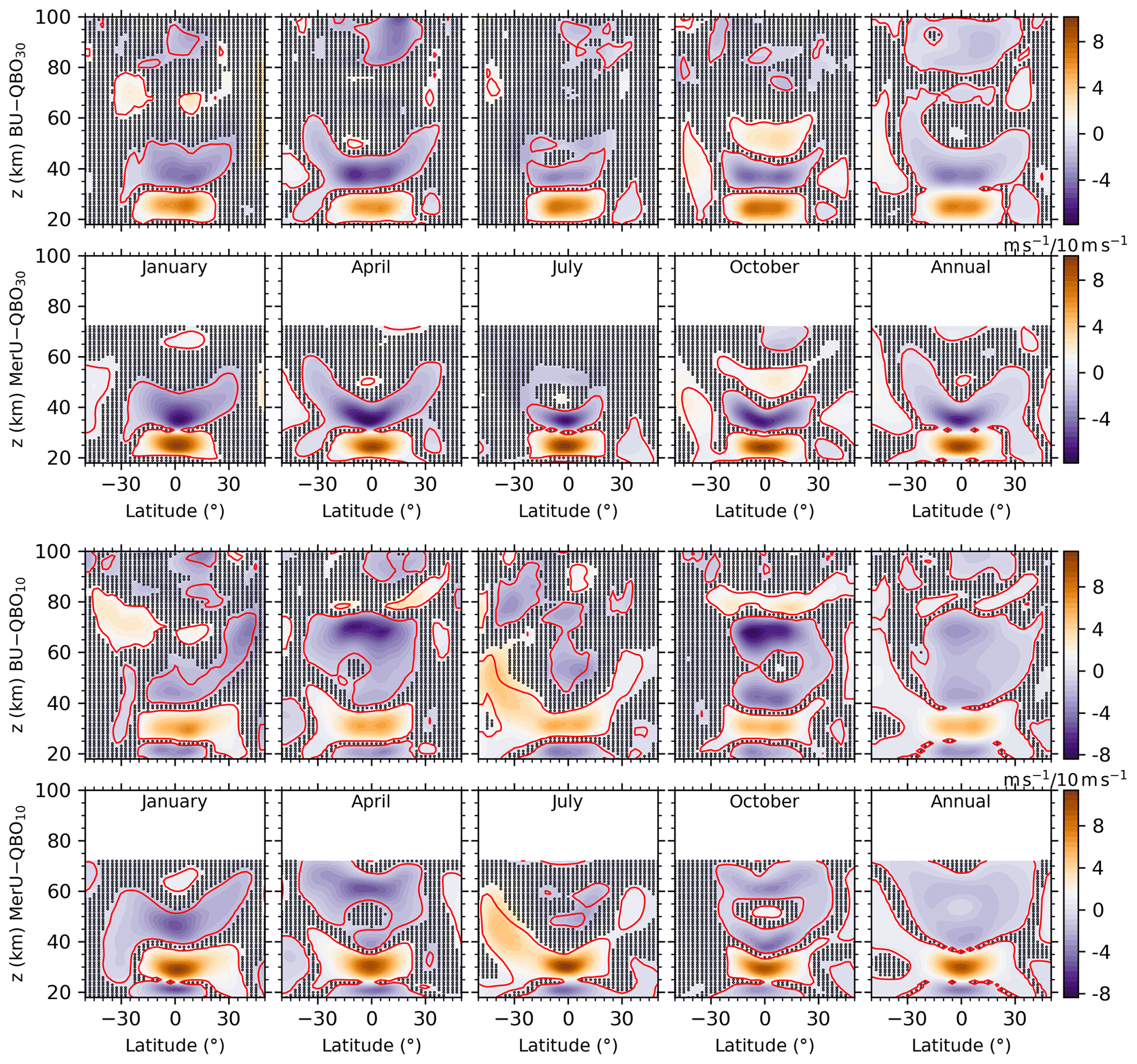
Figure 5 Same captions as the upper two rows of Fig. 4 but for the responses to QBO₃₀ (QBOB, upper two rows) and QBO₁₀ (QBOB, lower two rows).

The responses of BU to QBO₃₀ are weaker at ∼ 50–80 km. As the height increases, the responses of BU to QBO₃₀ become stronger again and have peak around ∼ 90 km. This coincides with the mesospheric QBO, which is anti-phase with the stratospheric QBO and extends to 30^∘ S–30^∘ N as revealed by High Resolution Doppler Imager observations (HRDI) (Burrage et al., 1996), revealed by TIMED Doppler Interferometer observations (Kumar, 2021), and reviewed by Baldwin et al. (2001). This coincides also with the results simulated by WACCM6 on the aspects of the hemispheric asymmetry, i.e., the responses extending to higher latitudes in winter hemisphere (Ramesh et al., 2020). Moreover, the annual mean responses of BU and MerU to QBO₃₀ and QBO₁₀ are positive and are significant at 50^∘ S at ∼ z = 50–80 km. In contrast, the responses of winds to QBO₃₀ and QBO₁₀ are negative and have smaller regions with p values less than 0.1. The significant positive responses at 50^∘ S are mainly contributed by those in July and October around 50 km, where and when the stratospheric polar jet occurred.

A short summary is that the influences of the stratospheric QBO extend from the Equator to higher latitudes. The influences can be positive or negative, which depend on heights and latitudes. Such as the negative influences above ∼ 80 km in the tropical region and the positive influences at the southern high latitudes. Above ∼ 80 km, the negative responses of winds to the stratospheric QBO are hemispheric asymmetry and are more negative in the NH tropical regions.

3.4 Responses to ENSO

The latitude–height distributions of the responses of BU and MerU to MEI (upper two rows of Fig. 6) generally coincide with each other in all months and in the annual mean. In January and at ∼ z = 40–60 km and latitudes higher than 40^∘ N, the responses of MerU and BU to MEI are not significant. This coincides with the results simulated by WACCM6, which were positive but were lower than the 95 % confidence level (Ramesh et al., 2020). In April and October, and at ∼ 35 km, the negative responses of winds to MEI are approximately hemispheric symmetric. The annual mean responses of both winds to MEI are stronger and wider in the SH than those in the NH. In July and at ∼ 50 km, the responses of both winds are positive with peaks around ∼ 40^∘ S. This indicates that the positive MEI index (warm phase of ENSO or El Niño event) increases the eastward zonal winds. Above 60 km, the positive responses of winds to MEI tilt from higher height (∼ 90 km) at 35^∘ S to a lower height (∼ 80 km) at 35^∘ N in January. This pattern continues in April and July but is insignificant. Above ∼ 90 km and around ∼ 15^∘ S, the responses of BU to MEI are positive in January and negative in July. The annual mean responses are mainly positive in most latitudes.

Figure 6 Same caption as Fig. 4 but for the responses to ENSO.

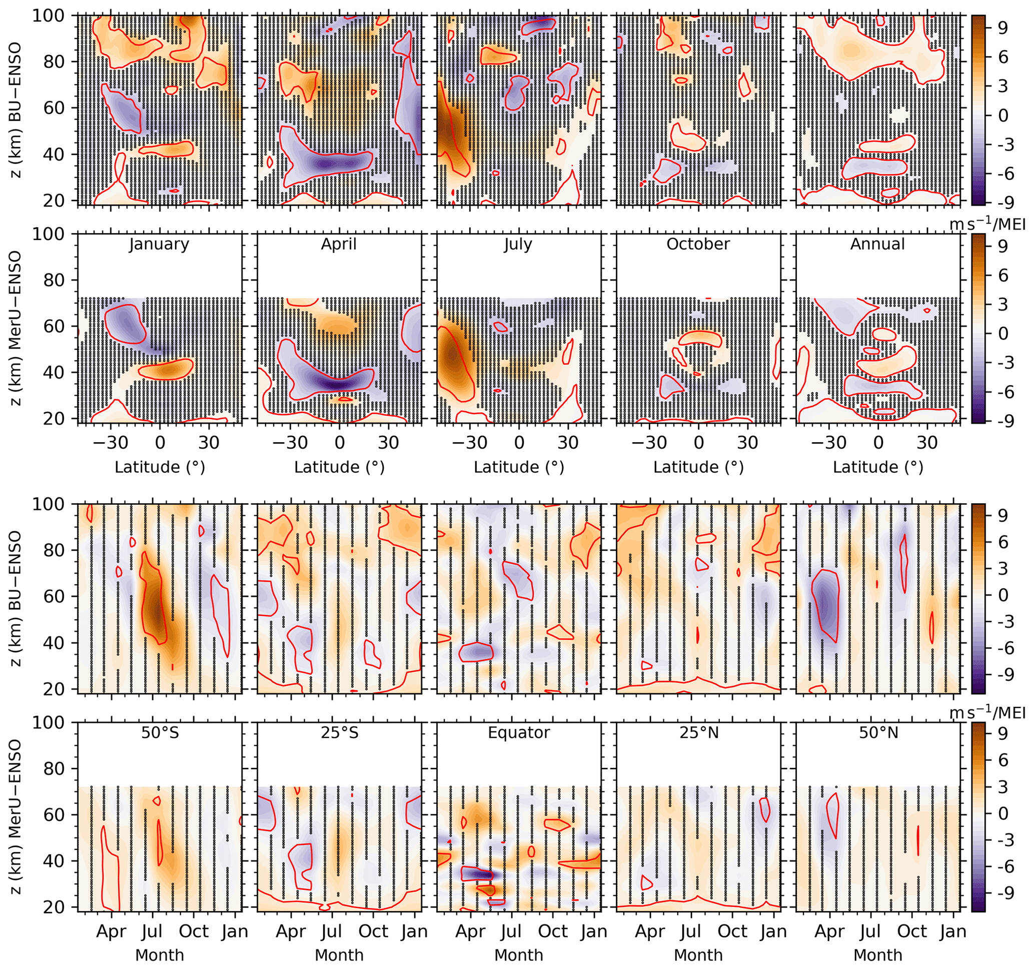
The monthly-height distributions of the responses of BU and MerU to MEI (lower two rows of Fig. 6) generally coincide with each other at each latitude, except that the responses of BU to MEI have stronger peaks than those of MerU at 50^∘ N/S. The prominent responses of winds to MEI are positive at 50^∘ S (tilting from July at higher height to October at lower height) and are negative at 50^∘ N (mainly in March and April). At 25^∘ N/S, the responses of winds to MEI are mainly positive (extending upward to ∼ 50 km and then tilting backward with the increasing height in July and August) and are negative (extending backward and forward below ∼ 60 km). At the Equator, the responses of MerU to MEI exhibit larger variabilities than those of BU below ∼ 40 km.

Previous studies showed that during El Niño (warm phase of ENSO), the warm sea surface temperature increases the wave activity, which has a high probability of leading to sudden stratospheric warming (SSW) events (Polvani and Waugh, 2004). Then the warm temperature and decelerated zonal wind anomalies can be observed in the stratosphere from January to April at 60^∘ N (Manzini et al., 2006; Domeisen et al., 2019). This can be summarized as a negative response of zonal wind to ENSO at northern high latitudes. This negative response can also be seen at 50^∘ N (two lower-right panels of Fig. 5). Using the WACCM simulations and SABER observations, Li et al. (2016) showed that the stratospheric zonal wind is weakened due to the increased stratosphere meridional temperature gradient at the southern high latitudes in December and in the warm phase of ENSO. This supports the weak negative responses of zonal wind to ENSO at 50^∘ S in December (lower-left two panels of Fig. 6). However, Both BU and MerU showed that the responses of zonal wind to ENSO are positive from July to October at 50^∘ S. The physics behind this positive response should be further explored through simulation studies.

It seems unusual that during July in the SH there is a strong signal in both F_10.7 and ENSO. A possible reason is that the waves (gravity waves, non-migrating tides, planetary waves) exhibit stronger variabilities and more complex spatial–temporal structures in the NH than those in the SH. This induces a more complex dynamical coupling between waves and zonal mean wind in the NH than that in the SH. Then the complex dynamical coupling might induce that influences of F_10.7 and ENSO to wind are not as obvious in the NH as in the SH. Another possible reason is that the zonal mean wind is stronger in the SH than that in the NH during wintertime. Thus, the responses of winds to F_10.7 and ENSO are stronger during July in the SH than those in the NH counterpart. Moreover, the responses of winds to QBO₁₀ are also stronger during July in the SH than those in the NH counterpart.

A short summary is that both BU and MerU exhibit similar responses to MEI, whereas the responses of BU to MEI are stronger than those of MerU at 50^∘ N/S. An interesting feature is that the responses of winds to MEI propagate downward with increasing time at 50 and 25^∘ N/S, especially the positive responses of BU to MEI at 50 and 25^∘ S.

3.5 Linear variations

The latitude–height distributions of the linear variations of BU and MerU (upper two rows of Fig. 7) generally coincide with each other in regions with p values smaller than 0.1. The consistencies include the following: (1) in January and around the Equator, the negative variations at ∼ 40 km and (2) in April and in the annual mean, the negative variations having peaks at 40^∘ N and extending to the northern higher latitudes. The discrepancies of the linear variations between BU and MerU include the following: (1) the negative variations of BU around 50^∘ N (50^∘ S) cannot be seen in MerU in January (April); (2) the positive variations of MerU are larger than those of BU above ∼ 55 km. Above 70 km, the patterns of the linear variations of BU are sporadic and insignificant and are strongly dependent on months, latitudes, and heights.

Figure 7 Same caption as Fig. 4 but for the linear variations.

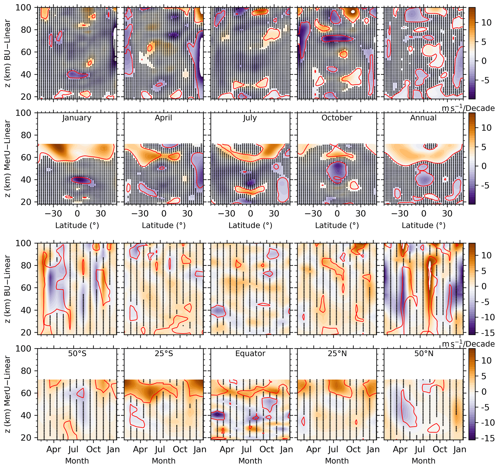
The monthly-height distributions of the linear variations of BU and MerU (lower two rows of Fig. 7) generally coincide with each other. The negative variations of BU and MerU coincide with each other but are insignificant at 50^∘ S in June–August and at 25^∘ S in March–May. However, the large discrepancy is that the negative variation of BU at 50^∘ N (but insignificant) cannot be seen in MerU in October–January. Above ∼ 70 km, the positive variations (but insignificant) last a longer time interval as compared to the negative variations.

Using the MF radar observations at Juliusruh (54.6^∘ N; 13.4^∘ E) during 1990–2005, Keuer et al. (2007) showed that the zonal wind below 80 km exhibited a negative trend of ∼ −5 m s⁻¹ per decade in summer and a positive trend of ∼ 4 m s⁻¹ per decade in winter (Fig. 14 of their paper). This result does not coincide with our analysis. By combining the radar, rocketsonde, and satellite observations over the Indian region and the simulation results by WACCM-X, Venkat Ratnam et al. (2019) show a negative trend of ∼ −5 m s⁻¹ per decade between 70 and 80 km. This result coincides with our analysis only during October. It should be noted that the linear variations of zonal wind depend on the stations, height ranges, measuring techniques, and the temporal intervals of the data (Keuer et al., 2007; Ramesh et al., 2020). This illustrates the complexity of the linear variations of zonal wind. Moreover, the inhibited linear variations of predictors used in the MLR model and the dynamics (such as SSW) are also important in retrieving the linear variations of zonal winds (Qian et al., 2019). The effects of the temporal coverage of the data and SSWs in the NH on the responses will be discussed in Sect. 4.

A short summary is that both BU and MerU exhibit similar linear variations. But this consistency is not as good as that of the seasonal variations or the responses to F_10.7, QBO, and ENSO. The large discrepancy is that the negative variations of BU at 50^∘ N cannot be seen in MerU in October and January. Above 70 km, the patterns of the linear variations of BU are sporadic and insignificant and are strongly dependent on months, latitudes, and heights.

4 Discussions

4.1 Influences of temporal intervals of data

Robust responses or linear variations should not depend on the temporal intervals of the data (Souleymane et al., 2021; Mudelsee, 2019; Qian et al., 2019). This means that the temporal interval of the data should be long enough, which is difficult to be satisfied since the atmospheric variations or oscillations have multiple temporal scales (ranging from months to decades). To test the robustness of the regression results described in Sect. 3, we change the temporal intervals of both BU and MerU according to solar activity, which exhibits nearly 11-year variations. One is 2002–2015, which covers an interval from solar maximum to minimum and then to maximum. The other is 2008–2019, which covers an interval from solar minimum to maximum and then to minimum. After August 2004, the MLS data have been assimilated into MERRA-2 (Molod et al., 2015; Gelaro et al., 2017). To test the sensitivity to this change, we introduce the third temporal interval of 2005–2019. Finally, the fourth temporal interval is 2002–2019, which is the entire data used here.

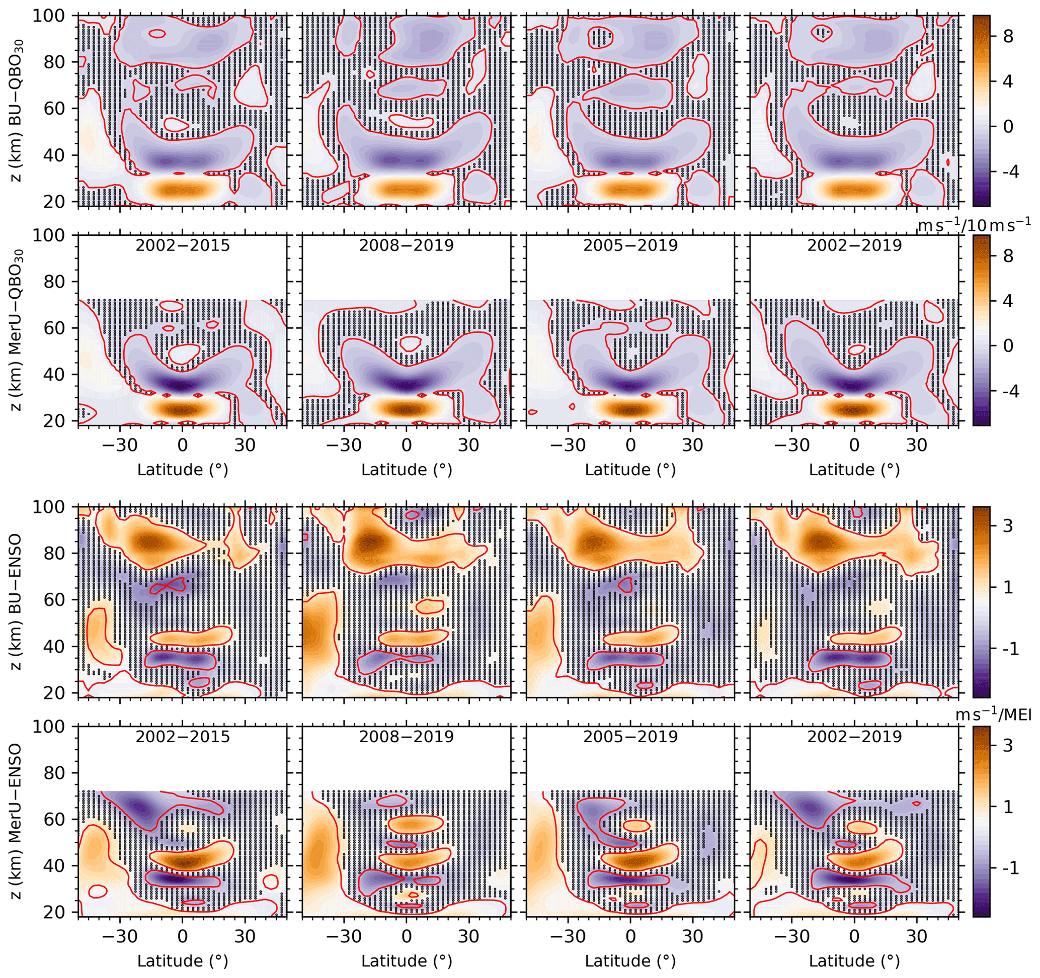
Figure 8 Latitude–height distributions of the annual mean responses of BU (the first and third rows) and MerU (the second and fourth rows) to QBO30 (upper two row) and ENSO (the lower two rows). The black dots indicate where the regression coefficients with p values larger than 0.2. The red lines indicate the regression coefficients with p values of 0.1.

Figure 8 shows the annual mean responses of winds to QBO₃₀ and ENSO in the four temporal intervals. The responses of BU to QBO₃₀ (the first row) are nearly identical among the four temporal intervals throughout the height range. The slight difference is the weaker positive responses of BU to QBO₃₀ during 2002–2015 and 2002–2019 at ∼ 70 km around the Equator. The responses of MerU to QBO₃₀ (the second row) are also nearly identical among the four temporal intervals throughout the height range. The slight difference is the weaker positive responses (insignificant) of MerU to QBO₃₀ at ∼ 50 km around the Equator during 2005–2019. These comparisons show that the responses of winds to QBO₃₀ are robust and are almost independent on the temporal intervals.

The annual mean responses of BU to ENSO (the third row) have similar patterns among the four temporal intervals, such as (1) the positive responses extending from the southern lower latitudes at lower height to higher latitudes at higher height, (2) the positive responses extend from the tropical regions at ∼ 40 km to middle latitudes at higher height, and (3) the positive and negative responses shifting with height in the tropical regions below ∼ 40 km. The slight difference is the weaker positive at the southern high latitudes and around ∼ 50 km during 2002–2015 and 2002–2019, as compared to the other two temporal intervals. The responses of MerU to ENSO (the fourth row) have also similar patterns of responses among the four temporal intervals. This is similar to that of BU and might be caused by the larger variabilities of MEI index after 2008. The negative responses of both winds to ENSO are stronger around ∼ 20^∘ S and ∼ 60 km during 2002–2015 and 2002–2019, as compared to other temporal intervals. In a word, the responses of winds to ENSO are robust but slightly depend on the temporal intervals. We note that the pancake structures in the responses of winds to QBO are likely induce by the propagation nature of QBO. Similar pancake structures can also be seen in the responses of wind to ENSO. Moreover, the pancake structures can also be seen in the responses of the zonal mean temperature to ENSO (Fig. 2 of Li et al., 2013). The physics behind should be further explored.

Figure 9 Same caption as Fig. 8 but for the responses to F_10.7 (upper two rows) and linear trend (lower two rows).

Figure 9 shows the annual mean responses of winds to F_10.7 (upper two rows) and the linear variations of winds (lower two rows) in the four temporal intervals. In the temporal intervals of 2002–2015 and 2002–2019, both BU and MerU exhibit similar responses to F_10.7. In the temporal intervals of 2008–2019 and 2005–2019, both BU and MerU also exhibit similar responses to F_10.7. In the four temporal spans, the responses of MerU to F_10.7 are more negative at latitudes higher than ∼ 30^∘ S and extend to a higher height than those of BU. Around the tropical region and at ∼ 40 km, the responses of MerU to F_10.7 are more negative than those of BU. At latitudes higher than ∼ 30^∘ S and around the tropical regions, the positive responses of BU to F_10.7 have peaks at ∼ z = 70–85 km, which are larger in the temporal intervals of 2002–2015 and 2002–2019, as compared to other temporal intervals. The stronger responses in the temporal intervals of 2002–2015 and 2002–2019 might be caused by the fact that the solar activity has a higher peak in 2002 than in 2014 (Fig. 1b).

The linear variations of both BU and MerU depend strongly on the temporal intervals and on the values at both edge points. Among the four temporal intervals, the regions and magnitudes of negative variations are largest and strongest in the temporal span of 2008–2019, are larger and stronger in the temporal interval of 2005–2019, and then are insignificant in the temporal interval of 2002–2019. In contrast, the regions and magnitudes of positive variations are largest and strongest in the temporal interval of 2002–2015. Because the dependencies of the linear variations of BU and their dependencies on different temporal interval are similar to those of MerU, we cannot determine whether or not the assimilation of MLS data into MERRA-2 influences the linear variations. The possible reasons, which are responsible for the strong dependencies of the linear variations on different temporal intervals, can be ascribed to the different linear variations inhibited in the predictors and the unstable predictors in different temporal intervals (Qian et al., 2019).

Table 2 Linear variations of F_10.7, QBO30, QBO10, and ENSO in different temporal spans and their combination effects on the linear variations of BU.

First, we examine the linear variations inhibited in the predictors (F_10.7, QBO, and ENSO) and list their linear slopes in Table 2. The values in Table 2 are approximate values and are derived through the following steps. From the upper two rows of Fig. 9, we see that the maximum response of winds to F_10.7 is 10 m s⁻¹ per 100 SFU (0.1 m s⁻¹ per SFU). According to this conversion rule, one unit of the linear variation of F_10.7 (SFU per decade) can induce the wind variation of 0.1 m s⁻¹ per decade. Approximately, one unit of the linear variation of ENSO (MEI per decade) can induce the wind variation of 1 m s⁻¹ per decade. Thus, in quality, the combination influences of these regressors can be summarized and listed in the last row of Table 1. We see that the inhibited linear variations of these regressors provide negative (positive) variations in the temporal spans of 2002–2015 and 2002–2019 (2008–2019 and 2005–2019). These inhibited linear variations share the linear variations of winds in Eq. (4). The positive (negative) inhibited linear variations make the linear variations winds more negative (positive). This is confirmed by the fact that the regions and magnitudes of linear variations decrease if we remove the linear variations of each regressors (not shown here). This explains partially the strong dependencies of the linear variations on different temporal spans.

Second, even if we remove the linear variation of each predictor, the dependencies of the linear variations on different temporal spans cannot be removed completely. This might be induced by the fact that the predictors are not stable time series and have varying magnitudes and periodicities in different temporal intervals, such as the MEI index, which has larger variabilities after 2009 than before (Fig. 1e), and F_10.7, which has larger peaks in 2002 than in 2014 (Fig. 1b). It should be noted that each predictor has its own linear variations and varying magnitudes and periodicities, which are the physical nature of the predictor and should not be removed, such that one can get a reliable response of the winds to each predictor although the responses depend on the temporal interval of the data.

The dependencies of winds to QBO are almost identical in different temporal intervals. The dependencies of winds to ENSO on temporal intervals are slightly stronger than to QBO. The dependencies of winds to F_10.7 on temporal intervals are stronger than to QBO. The dependency of the linear variations of winds on temporal intervals is the strongest one. Comparing among these responses and the linear variations, we can conclude that the MLR can capture robust responses if the predictor has relatively stable oscillation period and amplitude (i.e., QBO) and the data length is long enough to cover the main features of the predictor. The robustness decreases as the stability (i.e., the magnitudes and periodicities) of the predictor decreases (such as ENSO and F_10.7). For the linear variation, its oscillation period can be regarded as infinite. Thus, the data length should be infinite to get a reliable linear variation. However, this is not possible in reality. Consequently, we propose that the linear variations should be examined in different temporal spans, such that one can get a more comprehensive impression on the linear variations although the exact long-term linear variations are unknown.

To illustrate the influences on the temporal interval on the linear variations and responses, we performed the MLR procedure on the 40 years (1980–2019) of MERRA-2 data (MerU40, not shown here) to the results from 18 years (2002–2019) of MERRA-2 data (MerU18). Below ∼ 55 km, which is most reliable height since the damping is significant above this height (Ern et al., 2021), we find that the consistencies of the responses of MerU18 and MerU40 to QBO₃₀ and ENSO are better than those to F_10.7 and the linear variations. Moreover, at ∼ 40 km and around the Equator, the significant negative linear variations of MerU40 coincide well with those MerU18.

4.2 Possible reasons of hemispheric asymmetry

The responses of both BU and MerU to F_10.7 and ENSO exhibit hemispheric asymmetry. Specifically, the negative (positive) responses of winds to F_10.7 are stronger in the SH than those in the NH above the stratospheric polar jet region (around 80 km). The responses of winds to ENSO are positive and significant in the SH stratospheric jet region but are negative and insignificant in the NH counterpart. Above 80 km, the responses of BU to ENSO are more positive in the SH subtropical region than those in NH counterpart. The positive responses of winds to QBO extend to a wider latitude range in the SH stratospheric jet region than those in the NH counterpart. Moreover, the seasonal and linear variations of BU and MerU also exhibit hemispheric asymmetry. Specifically, the peaks of AO of both BU and MerU have larger amplitudes and at lower heights in SH than those in the NH. Although the linear variations of winds depend on the temporal intervals of data, the linear variations are hemispheric asymmetry on aspects of magnitudes and patterns in each temporal interval.

Since the predictor variables are same at all latitudes and heights, the hemispheric asymmetric responses should come from the hemispheric asymmetry of zonal winds. Figures 3 and 4 of Liu et al. (2021a) have shown that both BU and MerU were faster in the SH than those in the NH, especially when the wind is eastward in winter of each hemisphere. Moreover, the winds at middle and high latitudes of the SH were faster and more stable than those in the NH. One reason is that the SSW occurs frequently (6–7 times per decade) in the NH. During SSW, the eastward wind becomes weak or even reversal (Butler et al., 2015; Baldwin et al., 2021). We note that SSWs in the NH mainly occurred in the phase when the zonal wind was eastward (i.e., the zonal wind was eastward before and after SSWs, while the zonal wind becomes weak or reversed during SSWs). In contrast, the SSW rarely occurred in the SH (only 3 time during 2002–2019, i.e., major SSW in September 2002, minor SSWs in August 2010 and September 2019), mainly due to the weaker land–sea contrast and smaller planetary wave amplitudes in the SH than those in the NH (Eswaraiah et al., 2016; Li et al., 2021; Rao et al., 2020; Butler et al., 2015).

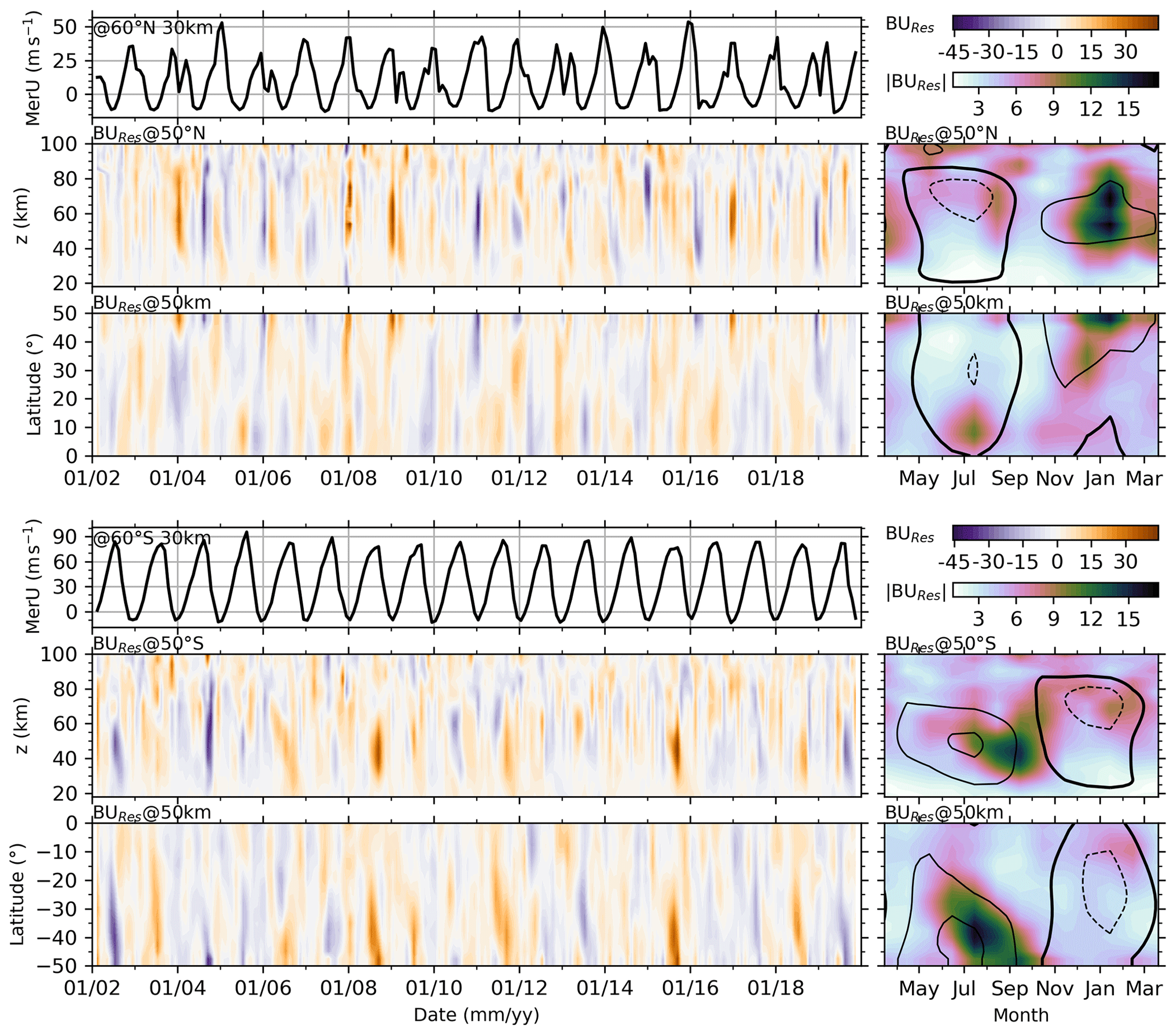
Figure 10 Upper three rows: MerU at 60^∘ N and 30 km (first row) and the residuals of BU (BU_res, the upper color bar in the top-right corner) at 50^∘ N (the second row) and 50 km (the third row), and the absolute values BU_res (|BU_res|, the lower color bar in the top-right corner) in a composite year. Lower three rows: same caption as the upper three rows but for the winds in the southern counterpart. The contour interval is 40 m s⁻¹. The westward, zero, and eastward winds are denoted by dashed, thick, and solid lines, respectively.

The MerU at 60^∘ N/S and 30 km (Fig. 10) shows that the SSWs in the NH have influence on the zonal wind at least in the monthly mean sense. However, the influence of SSWs on the zonal wind in the SH is neglectable. If we simply use the zonal wind at 60^∘ N/S and 30 km as a predictor to represent SSW, the prominent responses appear in summer but not in winter (when the SSW occur). This is because SSWs occur only in a limited temporal interval (1–2 weeks) in winter; the zonal wind at 60^∘ N/S and 30 km throughout the temporal interval includes both SSWs and other variations. It is desired to develop an index to represent the main features of SSW. This is out of the scope of this work and will be our future work. To illustrate the possible influences of SSWs on BU, we show in Fig. 10 the residuals of BU (BU_res) of Eq. (2) and their absolute values (|BU_res|) in a composite year. BU_res may represent the effects SSWs on BU to some extent since we did not include SSW as a regressor in Eq. (4).

From Fig. 10, we see that BU_res has larger magnitudes (positive or negative) in the NH when SSWs occur. Meanwhile, the magnitudes of BU_res decrease with the decreasing latitudes. |BU_res| in a composite year has a peak around January, when SSWs occur more frequently as revealed from the MerU at 60^∘ N. This indicates that the influences of SSWs on the regression results decrease with the decreasing latitudes in the NH. In contrast, BU_res has larger magnitudes when the zonal winds decelerate from their eastward peaks in the SH. Upon further examination on the |BU_res| in a composite year, we see that their peaks shift from September at 50^∘ S to July at lower latitudes. The larger |BU_res| in the SH is mainly due to the seasonal asymmetry of zonal winds; i.e., the zonal winds take a longer time to reach their eastward peak than that to reach their westward peak. The seasonal asymmetry of zonal winds might be induced by SAO and TAO.

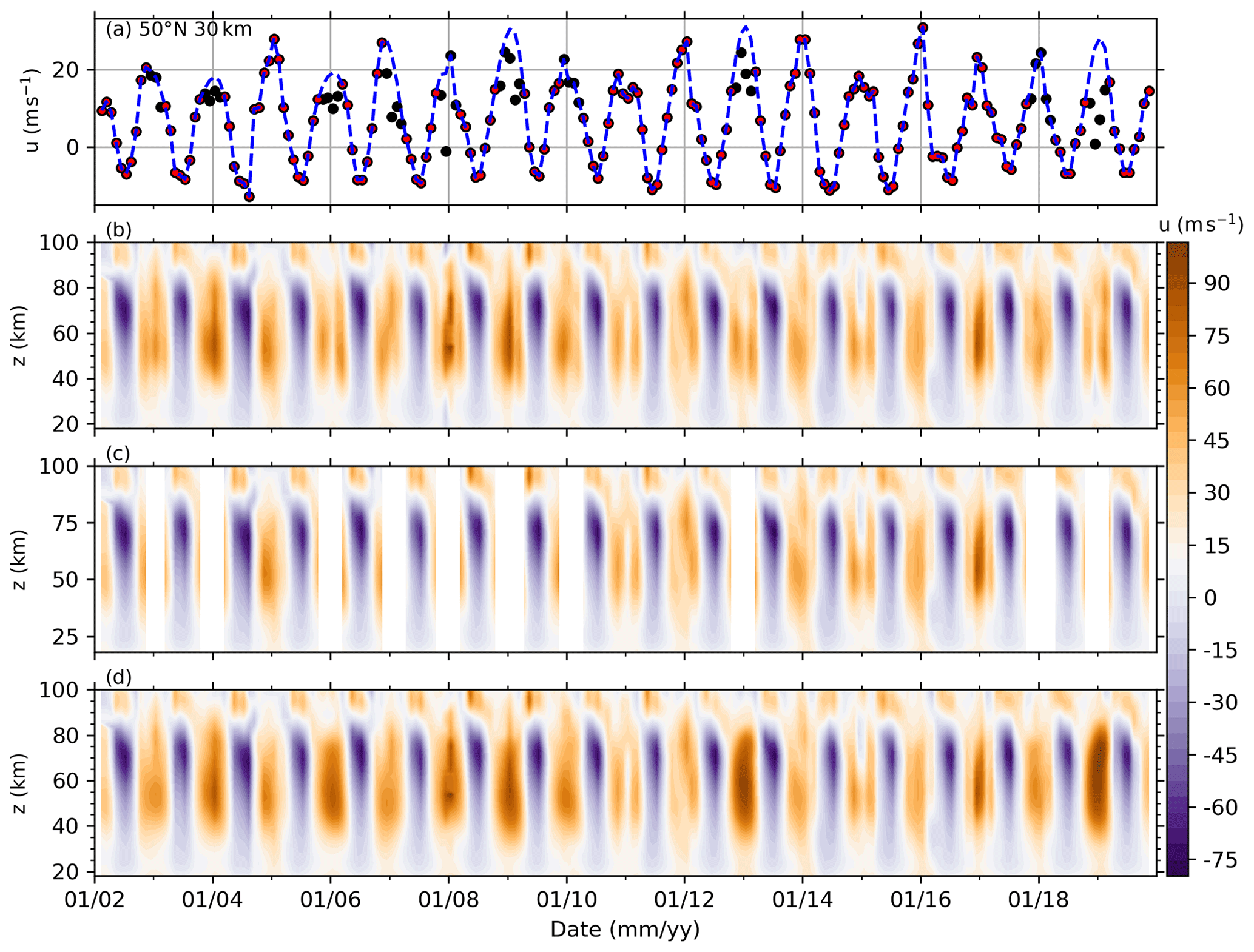
Figure 11 Removing SSWs from the raw BU and the reconstructed BU at 50^∘ N. (a) The remaining data (red dots), which are obtained by removing the data affected by SSWs from raw BU (black dots), and the reconstructed BU (blue dotted line, see text for detail). (b–d) The raw BU, remaining and reconstructed BU.

To test the possible influences of SSWs on the hemispheric asymmetry of the variations and responses, we reconstruct the BU in the NH during 2002–2019 through the following two steps. First, at each height of the NH, we remove the wind data during SSWs (i.e., the BU in winter does not increase monotonically before December or decrease monotonically after December, the specific years are 2003, 2004, 2006, 2007, 2008, 2009, 2013, 2018, 2019) from the raw wind (shown as black dots in Fig. 11a). Second, cubic spline interpolation is applied on the remaining data (red dots in Fig. 11a) to get a reconstructed wind series in winter (i.e., it increases monotonically before December and decreases monotonically after December, shown as blue dashed line in Fig. 11a). Figure 11b–d show the raw BU, remaining and the reconstructed BU, respectively. We see that the decelerated eastward winds during SSWs (Fig. 11b) have been replaced by the reconstructed BU; i.e., the eastward winds accelerate before December and decelerate after December (Fig. 11d). According to |BU_res| shown in Fig. 10, we reconstruct the BU at 30–50^∘ N and throughout the height range.

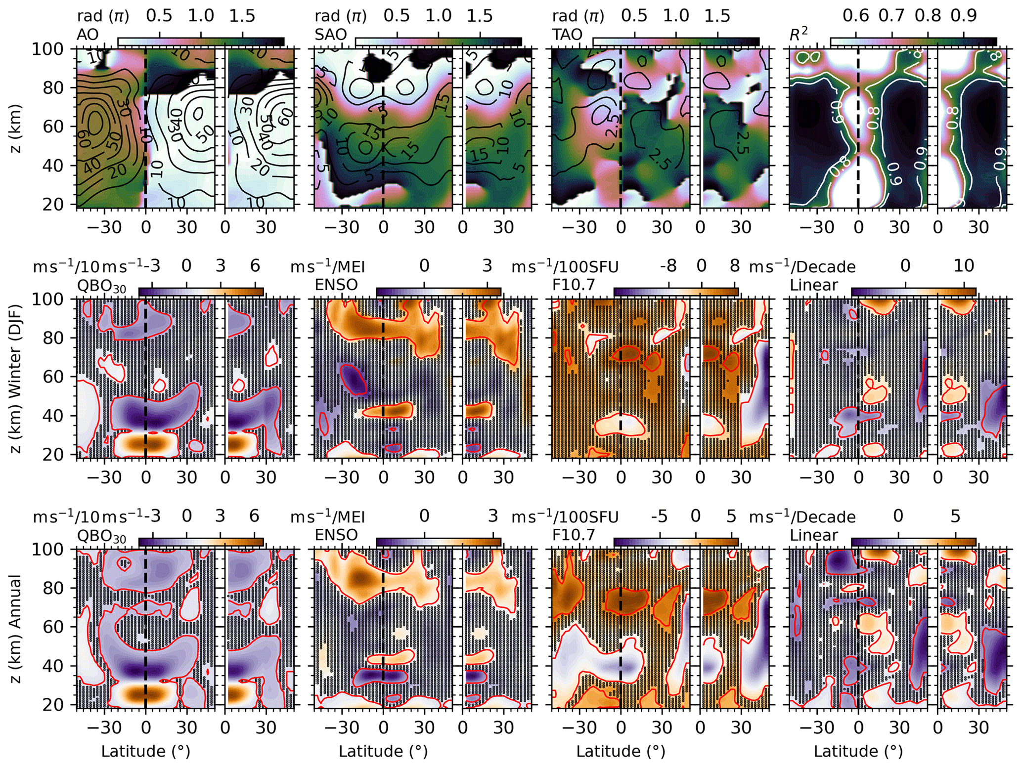
Figure 12 Regression results of the raw (50^∘ S–50^∘ N, left panel of each subplot) and reconstructed BU (0–50^∘ N, right panel of each subplot) in the NH during 2002–2019. Upper row: same caption as Fig. 3. Middle and lower row: same caption as Fig. 8 but for the responses of BU in winter (December–January–February) and in the annual mean, respectively.

Using the MLR procedure in Sect. 2.2, we performed the same regression on the reconstructed winds in the NH. Figure 12 shows the amplitudes of seasonal variations and R², and the responses of reconstructed winds to QBO, ENSO, F_10.7, and the linear variations. For comparison purposes, we also show in Fig. 12 the regression results of the raw BU. The R² indicates that Eq. (2) explains the reconstructed winds similar to the raw BU in the NH stratospheric polar jet region. The amplitudes of AO of the reconstructed winds are larger than those of the raw BU. However, the amplitudes of SAO and TAO of the reconstructed winds are smaller than those of the raw BU in the NH stratospheric polar jet region. Above 80 km, the amplitudes AO, SAO, TAO of both the reconstructed and raw BUs are nearly identical. This indicates that the influences of SSWs on the seasonal variations are mainly in the stratospheric polar jet region and around ∼ 65 km.

In winter, the response of the reconstructed and raw BU to QBO₃₀ and ENSO are similar in the aspects of both patterns and magnitudes. However, at ∼ 30–60 km and latitudes higher than 30^∘ N, the responses of the reconstructed BU to F_10.7 are more negative and significant. This is different from the positive and insignificant responses of the raw BU to F_10.7 in the same region. The linear variations of the reconstructed BU are significant and extend to a wider latitude but at a lower height than those of the raw BU.

The annual mean responses of the reconstructed and raw BU to QBO₃₀ and ENSO are similar in the aspects of both patterns and magnitudes. In contrast, at ∼ 30–60 km and latitudes higher than 30^∘ N, the annual mean responses of the reconstructed BU to F_10.7 are negative and positive, which cover the entire NH as compared to the responses of the raw BU. The linear variations of the reconstructed winds are more negative at latitudes higher than 30^∘ N as compared to linear variations of the raw BU.

In a word, compared to the raw BU, the reconstructed wind increases the amplitudes of AO but decreases the amplitudes of SAO and TAO in the NH stratospheric polar jet region. The responses of the reconstructed BU to QBO₃₀ and ENSO are similar to those of the raw BU on the aspects of both patterns and magnitudes and in the aspects of both winter and annual mean. However, at ∼ 30–60 km and latitudes higher than 30^∘ N, the responses of the reconstructed BU to F_10.7 and the linear variations of the reconstructed BU exhibit large differences as compared to the raw BU. However, the hemispheric asymmetry of the responses is not affected by SSWs at least in the monthly mean sense.

5 Conclusions

A global balance wind dataset (BU) is used to study the variations of the monthly zonal mean winds and the responses of the monthly zonal mean winds to solar activity, QBO, and ENSO at ∼ z = 18–100 km and 50^∘ S–50^∘ N and from 2002 to 2019. The variations and responses are extracted by MLR method after removing the collinearity of predictors, which is also applied to the MERRA-2 zonal wind (MerU) to test the reliability of BU and their responses.

The seasonal variations (AO, SAO, and TAO) of BU and MerU have nearly identical phases. The consistencies of their amplitudes are better in the SH than in the NH in the aspects of both patterns and magnitudes. The SAO of BU that has a peak around 80 km has hemispheric asymmetry and is stronger in the SH. The TAO of BU above 80 km also has hemispheric asymmetry and is stronger in the SH. The annual mean responses of BU and MerU to F_10.7 are more negative in the SH stratospheric polar jet region of SH than those of the NH counterpart. Around ∼ 80 km, the annual responses of BU to F_10.7 are mainly positive in the tropical region and high latitudes. The influences of the stratospheric QBO extend from the Equator to higher latitudes with increasing height. The influences can be positive or negative, which depend on heights and latitudes. Above ∼ 80 km, the negative responses of winds to the stratospheric QBO are hemispheric asymmetry and are more negative in the NH tropical regions. Both BU and MerU exhibit similar responses to MEI, whereas the responses of BU to MEI are stronger than those of MerU at 50^∘ N/S. The responses of winds to MEI propagate downward with the increasing time at 50 and 25^∘ N/S. Both BU and MerU exhibit similar linear variations. The large discrepancy is that the negative variations of BU at 50^∘ N cannot be seen in MerU during October–January. Above 70 km, the patterns of the linear variations of BU are sporadic and strongly dependent on months, latitudes, and heights.

The robustness of the responses of winds to QBO, ENSO, and F_10.7, and the linear variations of winds are examined by changing the temporal interval of the data. We found that the responses of winds to QBO are robust and are almost independent on the temporal intervals. The responses of winds to ENSO are robust but slightly dependent on the temporal intervals. Although the responses of wind to F_10.7 have similar patterns in different temporal intervals, the responses are stronger in the temporal intervals of 2002–2015 and 2002–2019 than the other two temporal intervals. The linear variations of both BU and MerU depend strongly on the temporal intervals. The possible reasons might be the different linear variations inhibited in the regressors and the unstable regressors in different temporal intervals. Thus, it is desired to examine the responses and linear variations in different temporal intervals, such that one can get a more comprehensive impression on the linear variations although the exact linear variations are unknown. The influences of SSWs on the seasonal variations are mainly in the NH stratospheric polar jet region. However, the hemispheric asymmetry of the seasonal and linear variations and the hemispheric asymmetric responses of BU to QBO, ENSO, and F_10.7 are not affected by SSWs at least in the monthly mean sense.