Investigating the radiative effect of Arctic cirrus measured in situ during the winter 2015–2016

The radiative energy budget in the Arctic undergoes a rapid transformation compared with global mean changes. Understanding the role of cirrus clouds in this system is vital, as they interact with short- and long-wave radiation, and the presence of cirrus can be decisive as to a net gain or loss of radiative energy in the polar atmosphere.

In an effort to derive the radiative properties of cirrus in a real scenario in this sensitive region, we use in situ measurements of the ice water content (IWC) performed during the Polar Stratosphere in a Changing Climate (POLSTRACC) aircraft campaign in the boreal winter and spring 2015–2016 employing the German High Altitude and Long Range Research Aircraft (HALO). A large dataset of IWC measurements of mostly thin cirrus at high northern latitudes was collected in the upper troposphere and also frequently in the lowermost stratosphere. From this dataset, we select vertical profiles that sampled the complete vertical extent of cirrus cloud layers. These profiles exhibit a vertical IWC structure that will be shown to control the instantaneous radiative effect in both the long and short wavelength regimes in the polar winter.

We perform radiative transfer calculations with the uvspec model from the libRadtran software package in a one-dimensional column between the surface and the top of the atmosphere (TOA), using the IWC profiles as well as the state of the atmospheric column at the time of measurement, as given by weather forecast products, as input. In parameter studies, we vary the surface albedo and solar zenith angle in ranges typical of the Arctic region. We find the strongest (positive) radiative forcing up to about 48 W m⁻² for cirrus over bright snow, whereas the forcing is mostly weaker and even ambiguous, with a rather symmetric range of values down to $-\mathrm{35}\mathrm{W}{\mathrm{m}}^{-\mathrm{2}}$, over the open ocean in winter and spring. The IWC structure over several kilometres in the vertical affects the irradiance at the TOA via the distribution of optical thickness. We show the extent to which IWC profiles with a coarser vertical resolution can reflect this effect. Further, a highly variable heating rate profile within the cloud is found which drives dynamical processes and contributes to the thermal stratification at the tropopause.

Our case studies highlight the importance of a detailed resolution of cirrus clouds and the consideration of surface albedo for estimations of the radiative energy budget in the Arctic.

1 Introduction

Cirrus clouds are ice clouds that exist at temperatures below the homogeneous freezing threshold of about 235 K. The required temperatures and humidity conditions are found in the upper troposphere and sometimes in the lowermost stratosphere, leading to an average global coverage of at least 20 %. Cirrus clouds form in ice supersaturated regions in the presence of suitable nuclei, such as solid or liquid aerosol, or via the freezing of (supercooled) liquid droplets in ascending air masses (Heymsfield et al., 2017).

The impact of cirrus on the radiative energy budget of the atmosphere can be differentiated into direct and indirect effects. The direct effect is absorption and re-emission of thermal (long-wave) radiation and scattering of solar (short-wave) radiation. Indirect or secondary effects arise from the redistribution of water vapour and through heterogeneous physical (e.g. trapping and release; Kärcher and Voigt, 2006; Kärcher et al., 2009; Voigt et al., 2006) and chemical reactions with radiatively active compounds, such as ozone-depleting substances (e.g. von Hobe et al., 2011; Solomon et al., 1997; Borrmann et al., 1996).

Cirrus occurrence and radiative properties are prone to anthropogenic influence through the introduction of ice-nucleating particles and precursors (Hoose and Möhler, 2012), including aircraft emissions (Kärcher, 2018), and via the evolution of atmospheric humidity as a feedback to changing climate as a whole. It is known that the microphysical properties of cirrus, such as the particle number concentration, size distribution and shape, depend on the nuclei and the environmental conditions during nucleation, such as updraft speeds (e.g. Kärcher and Jensen, 2017; Joos et al., 2014; Krämer et al., 2020).

Cirrus clouds are more abundant and thicker in the tropics and at midlatitudes, but there is also considerable coverage in the high-latitude and polar regions. In these areas, the low elevation of the sun and the complete absence of sunlight during polar nights reduce the short-wave effect (Hong and Liu, 2015). In addition, the Arctic surface climate is currently undergoing a much more rapid warming transition than the rest of the globe, known as Arctic amplification, which also changes the spatial and temporal patterns of the surface albedo as sea ice and continental ice retreat (Wendisch et al., 2017; Shupe et al., 2022). Therefore, the question of how Arctic cirrus clouds impact (will impact) the radiation budget now (and in the future) has not yet been answered satisfactorily. Furthermore, the direction, extent and circumstances under which the cirrus feed back to the current warming are unknown.

Although cirrus clouds are regularly observed from space with active (e.g. Sassen et al., 2008; Pitts et al., 2018) and passive (e.g. Strandgren et al., 2017) sensors, in situ measurements are needed for the closure of the physical appearance of cirrus ice crystals and their bulk radiative properties (Thornberry et al., 2017; Krisna et al., 2018; Ewald et al., 2021). There have been some in situ studies on Arctic cirrus clouds in the past, including the following: the Polar Stratospheric Aerosol Experiment (POLSTAR) missions in 1997 and 1998 (Schiller et al., 1999), the European Polar Stratospheric Cloud and Lee Wave Experiment (EUPLEX) in January–February 2003 and the ENVISAT validation experiments in October 2002 and March 2003, which all produced measurements of the ice water content (IWC) up to 68^∘ N (summary in Schiller et al., 2008), and the Stratospheric Aerosol and Gas Experiment (SAGE) III Ozone Loss and Validation Experiment (SOLVE) in 1999–2000, which produced measurements of the IWC and particle size distribution (Schiller et al., 2002; Hallar et al., 2004). The mentioned missions accumulate to a total of 15 flights and significantly contributed to our current picture of cirrus in the Arctic. Nevertheless, these are few studies compared with the much more comprehensive observations in the tropics and at midlatitudes (e.g. Voigt et al., 2007; Thornberry et al., 2017; Heymsfield et al., 2017; Krämer et al., 2016, 2020).

An earlier study by Feofilov et al. (2015) used spaceborne radar, lidar and radiance measurements to derive the radiative impact at the top of the atmosphere (TOA) of differently shaped IWC profiles including global variations. Although we also examine this effect for the inhomogeneous vertical IWC distributions in our measurements, our study focuses on high-latitude cirrus, and we demonstrate the radiative effects, including the heating rate, in the entire atmospheric column. This also constitutes a link to cloud dynamics modelling studies that investigate the interaction of heating rate profiles with ice supersaturation, vertical velocity, and particle nucleation and growth (Fusina et al., 2007; Fusina and Spichtinger, 2010). Bucholtz et al. (2010) present directly measured heating rates in thin tropical cirrus and highlight the importance of further observations to improve the understanding of the radiative effects of cirrus.

The present work introduces a novel dataset of in situ IWC measurements carried out during the Polar Stratosphere in a Changing Climate (POLSTRACC) campaign employing HALO, the German High Altitude and Long Range Research Aircraft (Oelhaf et al., 2019). The campaign was based in Kiruna (67.5^∘ N, 20.3^∘ E), Sweden, and spanned the boreal winter–spring season from 17 December 2015 to 18 March 2016 with 18 science flights and 156 flight hours. The campaign accommodated a number of different science goals, including trace gas composition in the upper troposphere and lower stratosphere (Marsing et al., 2019; Johansson et al., 2019; Braun et al., 2019; Keber et al., 2020; Ziereis et al., 2022), gravity waves (Krisch et al., 2020) and polar stratospheric clouds (Voigt et al., 2018). Therefore, the flight strategy often needed to avoid extended sections in cirrus clouds. Nevertheless, a total of 7.2 h or 5600 km inside cirrus during 44 individual events was recorded.

The flights included several climb or descent profiles through cirrus clouds, predominantly located just below the thermal tropopause. In this study, we take advantage of these IWC profiles and embed them in the corresponding atmospheric column of temperature and trace gases from the European Centre for Medium-Range Weather Forecasts (ECMWF) model analysis. We investigate the location of cirrus in relation to the local tropopause and the characteristic of a tropopause inversion layer (TIL) above. In a second step, this enables radiative transfer calculations that help understand the effect of these high-latitude ice clouds on the atmospheric radiation budget as a whole and on the heating rate profile inside the cloud layer in detail. This constitutes the link between realistic profiles (as they are directly measured) and their impact on local dynamics and the radiative energy budget.

The paper is laid out as follows: Sect. 2 contains the experimental acquisition of the in situ IWC data; an overview and the statistical characteristics of sampled Arctic cirrus clouds are given in Sect. 3; Sect. 4 breaks the observations down to the detailed profiles; Sect. 5 elaborates on the radiative transfer calculations; Sect. 6 contains a discussion of the findings and conclusions drawn from the material; and Sect. 7 closes with a short outlook.

2 In situ measurements of the IWC

The IWC is a derived quantity from our bulk measurements of the total atmospheric water content (TWC), which consists of the gaseous (vapour) phase and condensed phases (liquid and ice). In the present closed-path principle, a sample airflow was led into the aircraft cabin and heated, in order to evaporate all water content. The TWC measurement was then performed with the WAter vapoR ANalyzer (WARAN) laser hygrometer. This instrument derives the concentration of water vapour in the sample flow by using the absorption of the 1.37 µm line from an indium–gallium–arsenide (InGaAs) tunable diode laser (TDL) in a closed measurement cell (Voigt et al., 2014). The sensor is the commercial WVSS-II system (SpectraSensors Inc.) with a modified stainless-steel inlet line, and it is connected to a forward-facing trace gas inlet (TGI) with a 9.55 mm diameter at 31.9 cm distance from the fuselage of HALO. The measurement range is 50–10000 ppmv, with a precision of 5 % or 50 ppmv, whichever is greater. Values are sampled at a frequency of 0.3–0.4 Hz.

Although the instrument design and data treatment compensate for drifts due to changing environmental conditions, such as temperature and pressure (Heller, 2018), slow degradation requires repeated calibration within months. A calibration for the POLSTRACC campaign was performed afterwards on 28 July 2016 using a gauged dew point mirror (MBW 373-LX). The result is a linear correction function:

$$\begin{array}{}\text{(1)}& {\mathrm{H}}_{\mathrm{2}}{\mathrm{O}}_{\mathrm{calibrated}}=a+b\cdot {\mathrm{H}}_{\mathrm{2}}{\mathrm{O}}_{\mathrm{WARAN}},\end{array}$$

where H₂O_WARAN denotes the output water vapour mixing ratio from WARAN, and H₂O_corrected is the calibrated mixing ratio (both in ppmv). The calibration coefficients a and b are determined piecewise:

$$\begin{array}{}\text{(2)}& \begin{array}{ll}a=& \mathrm{3.756}\mathrm{ppmv},b=\mathrm{1.045}\\ & \text{for}{\mathrm{H}}_{\mathrm{2}}{\mathrm{O}}_{\mathrm{WARAN}}\le \mathrm{70}\mathrm{ppmv};\\ a=& \mathrm{12.619}\mathrm{ppmv},b=\mathrm{0.944}\\ & \text{for}{\mathrm{H}}_{\mathrm{2}}{\mathrm{O}}_{\mathrm{WARAN}}>\mathrm{70}\mathrm{ppmv}.\end{array}\end{array}$$

In cirrus clouds that contain only ice, the ice water content (IWC) can be calculated by subtracting the gas-phase water content (GWC) from the measurement. Due to the lack of an independent GWC measurement in clouds during the POLSTRACC campaign, the saturation mixing ratio is used as a first-order approximation, calculated from the Clausius–Clapeyron equation, as in Heller (2018). In reality, the relative humidity with respect to ice (RH_i) inside cirrus mostly assumes values between 80 and 120 %. Stronger sub- and particularly supersaturations, up to the homogeneous freezing threshold (about 150–165 %), are possible wherever particle growth rates are too slow to mitigate the excess relative humidity (Krämer et al., 2020). Such pronounced supersaturation has an increased probability at temperatures below 200 K, where cirrus clouds are often characterised by initially low particle number concentrations (Krämer et al., 2020). High supersaturation is strongly correlated with high updraft speeds, which eventually trigger homogeneous nucleation (Krämer et al., 2009) with a rapid increase in the particle number concentration (Mitchell et al., 2018). Updraft speeds for the selected cases in the sections below reach rather high values of up to about 0.5–1 m s⁻¹. This increases the expected quasi-steady-state relative humidity (Krämer et al., 2009) in the relevant temperature range to up to 120–130 %. Krämer et al. (2009) note that relaxation times towards this state are concurrently reduced at higher updrafts from a few to tens of minutes; thus, supersaturation depends strongly on the timing of the observation within the cirrus life cycle. This natural climatological variability propagates into the uncertainty of the calculated IWC, but the effect is strongly mitigated by the particle sampling characteristics explained in the following.

Sub-isokinetic sampling due to a lower inlet flow velocity (around 3 m s⁻¹) compared with the speed of airflow around the fuselage (typically around 230–240 m s⁻¹) leads to an inertial enhancement of particles in the inlet flow. Therefore, a correcting “enhancement factor” (EF) needs to be applied to the IWC measurement. Following the rationale in Heller (2018), the EF for typical high-latitude cirrus, where significant contributions to the IWC are contained in particles with radii larger than 20 µm (Wolf et al., 2018), can be calculated as

$$\begin{array}{}\text{(3)}& \mathrm{EF}={\displaystyle \frac{u_a}{u_{\mathrm{0}}}}\end{array}$$

with the known airspeed u_a and inlet velocity u₀ (Schiller et al., 1999). This approximation is independent of the precise particle size distribution and uses values of about 70 to 80 for the POLSTRACC measurements. Such high EF values effectively lower the detection limit of the corrected IWC to below 1 ppmv. The error in calculating the EF is ± 5 %, leading to a precision of 10 % for the IWC measurements. With this enhancement of the IWC over the GWC, if we were to assume a hypothetical supersaturation of RH_i = 160 % instead of 100 %, the IWC in the cases below would be reduced by a factor of 0.002–0.03 on 25 January 2016 (and by a factor of 0.04–0.14 on 9 March 2016). This is the uncertainty associated with the saturation assumption made above, ranging from negligible within the instrument errors to about 14 % in case of maximum supersaturation.

Figure 1 Comparison of the ice water content (IWC) from the WAter vapoR ANalyzer (WARAN) and Fast In-situ Stratospheric Hygrometer (FISH) instruments for cirrus measurements during the POLSTRACC campaign. The shading indicates the distribution of data within each WARAN bin. Note the double logarithmic axes and the logarithmic colour scale. The solid line represents the 1:1 identity. The dashed lines denote a deviation of a factor of 2, and the dotted lines denote a deviation of a factor of 10. Accounting for the detection limit, WARAN data are clipped below 0.2 ppmv.

Another major uncertainty in the airborne IWC measurements arises from further enhancement or depletion of particles of different sizes in the flow around the aircraft before they reach the sampling position. Afchine et al. (2018) studied this effect in detail, including data from the Midlatitude Cirrus (ML-CIRRUS) HALO mission (Voigt et al., 2017), and found particular ramifications for cabin instruments with inlet positions at the fuselage. Afchine et al. (2018) found that the IWC from WARAN was mostly systematically higher than the IWC from the Fast In-situ Stratospheric Hygrometer (FISH, Meyer et al., 2015), a Lyman-α hygrometer that samples total water in a similar way but at a different position. This comparison is repeated with the POLSTRACC data in Fig. 1. Here, a systematic deviation is not obvious, as the correlation between both instruments is well centred on the 1:1 line and there are no pronounced off-centre branches. More than 50 % of the measurements coincide within a factor of 2 above 1 ppmv. In a linear regression, the coefficient of determination R²=0.73 is smaller compared with that reported by Afchine et al. (2018), but the intercept $y_{\mathrm{0}}=-\mathrm{0.040}$ is closer to zero and the slope m=0.952 closer to identity. This enhanced comparability is attributed to improved calibration and a precise synchronisation of data streams. It also shows that the different positions of both inlets, which are about 3 m apart along the length of the fuselage, have a less pronounced impact on the observable IWC than previously thought. Nevertheless, we need to clarify that the IWC measurements from both instruments through roof-mounted TGIs are strongly affected by the enrichment or loss of ice particles due to their inertia in the flow around the aircraft's fuselage. Afchine et al. (2018) could quantify this effect for the HALO aircraft by comparing the IWC and particle size distribution measurements at the much less affected wing probe position, where IWC deviations of up to 1 order of magnitude were observed at a significant frequency. This flaw cannot be easily overcome for the POLSTRACC data without knowledge about the particle size distribution. Therefore, in the study of the impact of the observed IWC distributions on radiation in Sect. 5, we address the effects of underestimated IWC sampling. There, we test the sensitivity of our results to an underestimated IWC by re-evaluating all calculations with IWC profiles multiplied by a factor of 5, which corresponds to the average deviation seen for the FISH instrument in the worst particle size regime above 25 µm (Afchine et al., 2018).

3 Statistics of Arctic cirrus sampling

The POLSTRACC mission accommodated several scientific objectives that made use of the high-ceiling-altitude, long-range and heavy-payload capabilities of the HALO research aircraft (Oelhaf et al., 2019). For the observation of trace gas composition and gravity waves, the flight strategy often needed to avoid extended in-cloud sections. Therefore, the dataset represents a relatively random sampling of cirrus at the middle to high latitudes. Nevertheless, the 18 science flights spanning 156 flight hours yielded an accumulated residence time of 7.2 h inside cirrus clouds during 44 individual events, as calculated from the number of WARAN IWC measurements at temperatures below 235 K.

Figure 2 shows the IWC measurements as coloured sections of the POLSTRACC flight tracks. It can be seen that there are many shorter sections around the landing sites during the campaign, including the following: Oberpfaffenhofen, Germany (EDMO); Kiruna, Sweden (ESNQ); and Kangerlussuaq, Greenland (BGSF). Cloud layers in these sections were often crossed during approaches and departures. Some more extended sections in mid-flight are found intermittently. The colour coding shows the range of temperatures during these cirrus encounters. The minimum temperature recording during an IWC event was 195.8 K.

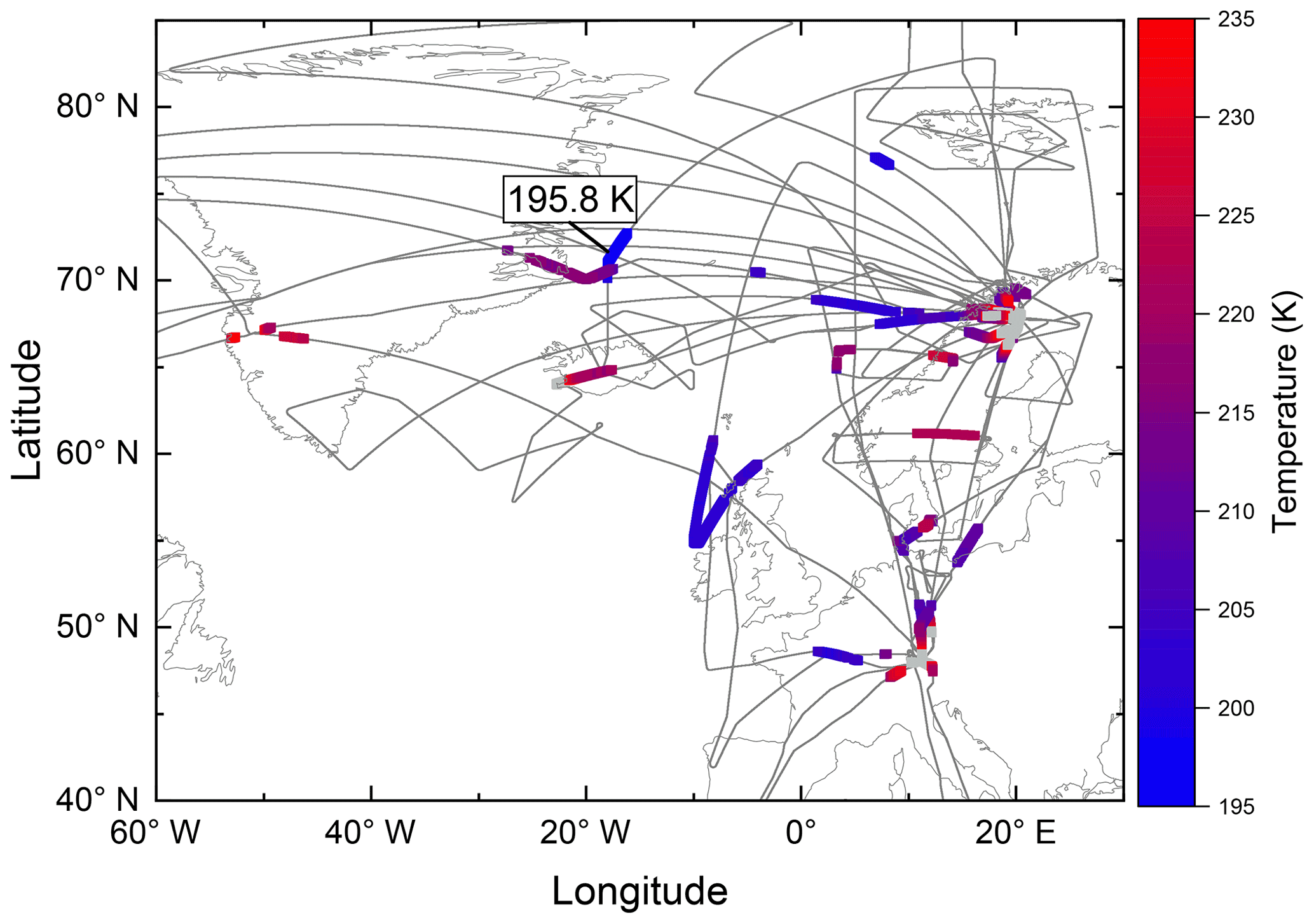
Figure 2 Map of the North Atlantic showing the flight tracks of the POLSTRACC campaign. Coloured sections denote the IWC measurements from the WARAN instrument. The colour coding indicates the temperature during these sections: red is warmer than blue, and grey colours are above 235 K.

With respect to the IWC as an accessible bulk property, previous studies have set up climatologies that relate the IWC to temperature (Schiller et al., 2008; Krämer et al., 2016) and other properties, such as effective radius and number concentration (e.g. Krämer et al., 2020; Luebke et al., 2013; Liou et al., 2008), and have broken them down to different latitudes on Earth and different cloud formation pathways. Schiller et al. (2008) and later Luebke et al. (2013) collected the range of airborne cirrus measurements from different campaigns as a function of latitude and temperature. In Fig. 3, the POLSTRACC measurements are added to this scheme found in Luebke et al. (2013). The broad latitudinal range of the POLSTRACC measurements can be seen. Although many domains have been covered by previous missions, Fig. 3 shows that the new data also extend into gaps that were not filled before. In particular, this concerns the lower temperatures below 210 K down to 198 K in the midlatitudes between 45 and 60^∘ N. A 4 h fraction of the campaign data was sampled north of 60^∘ N, and a significant extension to existing data could be made at 65^∘ N over the whole temperature range. Measurements north of 70^∘ N are generally sparse, and POLSTRACC can extend the coverage slightly for cold cirrus below 200 K. However, coverage is still sparse with respect to temperature and in the latitudinal range between 70^∘ N and the pole.

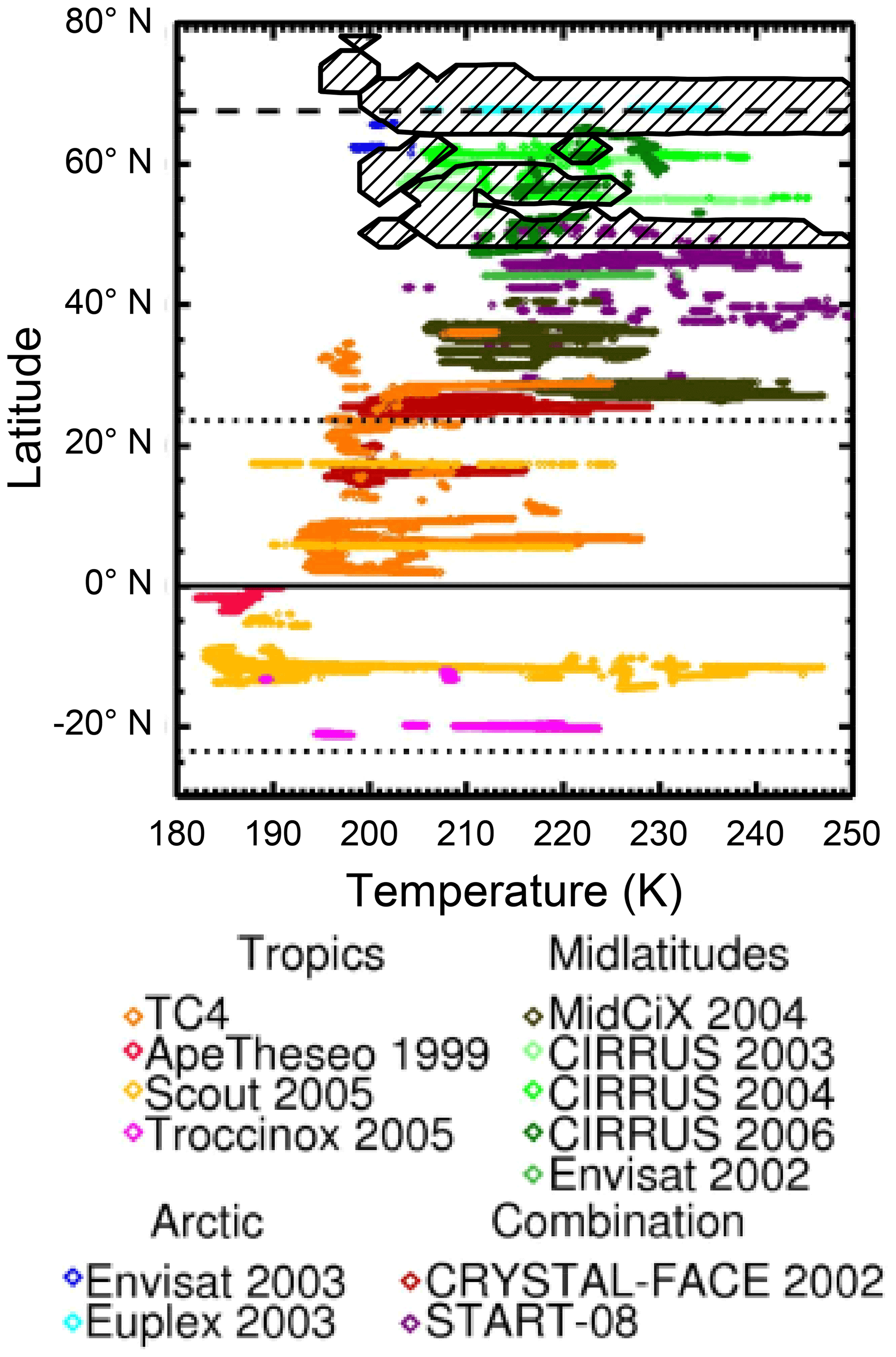
Figure 3 The black contour and diagonal stripes sketch the coverage of cirrus measurements during POLSTRACC with respect to latitude and temperature. For this work, the original of this figure from Luebke et al. (2013) is adapted, showing the coverage of airborne in situ cirrus missions from the literature.

Since the creation of the original figure by Luebke et al. (2013), the POLSTRACC observations represent the only addition of airborne in situ data at northern polar latitudes. Further observations not included in this figure comprise, for example, the previously mentioned ML-CIRRUS campaign at midlatitudes (Voigt et al., 2017).

This study focuses on cirrus near the tropopause. We examine the distribution of cirrus sampling along different tropopause-related vertical coordinates, which helps to assess the role of the geometrical location and extent, as well as temperature, in the cloud radiative effect, which at the tropopause becomes especially relevant in view of thermal stratification. Furthermore, different formation pathways and ice particle properties are expected for tropospheric and stratospheric cirrus. The following discussion is limited to observations north of 60^∘ N. Figure 4a displays the cirrus observations using two vertical scales: the abscissa indicates the potential temperature difference d_TP of the observation location to the 2 PVU (potential vorticity unit, $\mathrm{1}\mathrm{PVU}={\mathrm{10}}^{-\mathrm{6}}\mathrm{K}{\mathrm{m}}^{\mathrm{2}}{\mathrm{kg}}^{-\mathrm{1}}{\mathrm{s}}^{-\mathrm{1}}$) isosurface of potential vorticity (often denoted as dynamical tropopause), which is typically located at a potential temperature of 300–320 K (but a further ±10 K is possible). The ordinate axis indicates the squared Brunt–Väisälä frequency (N²) as a measure of the static stability of the atmospheric thermal stratification. The colour coding indicates the temperature as in Fig. 2. Close to the tropopause, roughly linear correlations between d_TP and N² can be observed, connecting the free, statically less stable troposphere with $N^{\mathrm{2}}<\mathrm{2}\times {\mathrm{10}}^{-\mathrm{4}}$ s⁻² to the stratosphere with $N^{\mathrm{2}}>\mathrm{4}\times {\mathrm{10}}^{-\mathrm{4}}$ s⁻². This correlation is not compact but spans a corridor with a width of 7 to 10 K. The lower-right branch belongs to January mid-winter measurements, whereas the upper-left branch stems from the March late-winter measurements. This may be interpreted as an increasing stabilisation of the tropopause region within 2 months due to the steady descending motion in the stratosphere (Manney and Lawrence, 2016; Birner, 2010). The blue colours highlight the occurrence of cold cirrus at T≲200 K above the dynamical tropopause. In most cases, these cirrus clouds on the stratospheric side have no continuation in the troposphere. They build up a lower branch of polar stratospheric ice clouds (PSCs) and do not rely on a tropospheric water vapour supply. Ice nucleation, particle size and habit as well as chemical constitution differ significantly from the tropospheric tropopause cirrus, and they play a crucial role in heterogeneous chemistry in the lowermost stratosphere, especially impacting the budgets of ozone-depleting substances. Figure 4b shows the distribution of measurements with respect to N². Two major accumulation regions can be identified: one at $\mathrm{2}\times {\mathrm{10}}^{-\mathrm{4}}$ to $\mathrm{3}\times {\mathrm{10}}^{-\mathrm{4}}$ s⁻² and another at $\mathrm{4}\times {\mathrm{10}}^{-\mathrm{4}}$ to $\mathrm{5}\times {\mathrm{10}}^{-\mathrm{4}}$ s⁻². The former can be attributed to tropospheric cirrus extending up until the thermal tropopause (according to the definition from the World Meterological Organization, WMO; World Meteorological Organization, 1957) and the latter to stratospheric cirrus with no or only a weak connection to the troposphere.

The distribution of cirrus observations can also be related directly to potential vorticity (PV), as seen in the bars in Fig. 4c. As already indicated above, a PV of 2 PVU is usually chosen as the dynamical tropopause and follows other tropopause definitions adequately in areas of weak horizontal wind shear, although it is located systematically below the thermal tropopause (Gettelman et al., 2011). For the extratropics a value of 3.5 PVU is often more consistent with the thermal tropopause (Hoinka, 1997). In Fig. 4, the low counts in the 0 to 0.5 PVU range may suggest a low cloud occurrence in the mid-troposphere. This is not necessarily the case and may be a result of the artificial limitation of the data to temperatures below 235 K, which has been applied in order to exclude false hits from mixed-phase clouds. Therefore, certainly more clouds were encountered there, composed of pure ice, mixed phases or liquid water. The highest cirrus occurrence is found below the 2 PVU isosurface with a maximum at 1–1.5 PVU, which is unambiguously located in the troposphere, where the available water vapour content is still at least 1 order of magnitude above stratospheric values. Higher up, cirrus sampling steadily decreases towards a rather uniform distribution above the 3.5 PVU isosurface. This reflects a random distribution of cirrus observations in the stratosphere, where PV varies strongly in the vertical direction and no single level is preferred for cirrus occurrence. Among the generally low IWC sampling frequency in the stratosphere, the apparent rise between 6 and 8 PVU is most likely due to the overall distribution of flight time in the stratosphere during the campaign, as can be seen by the black line in Fig. 4c.

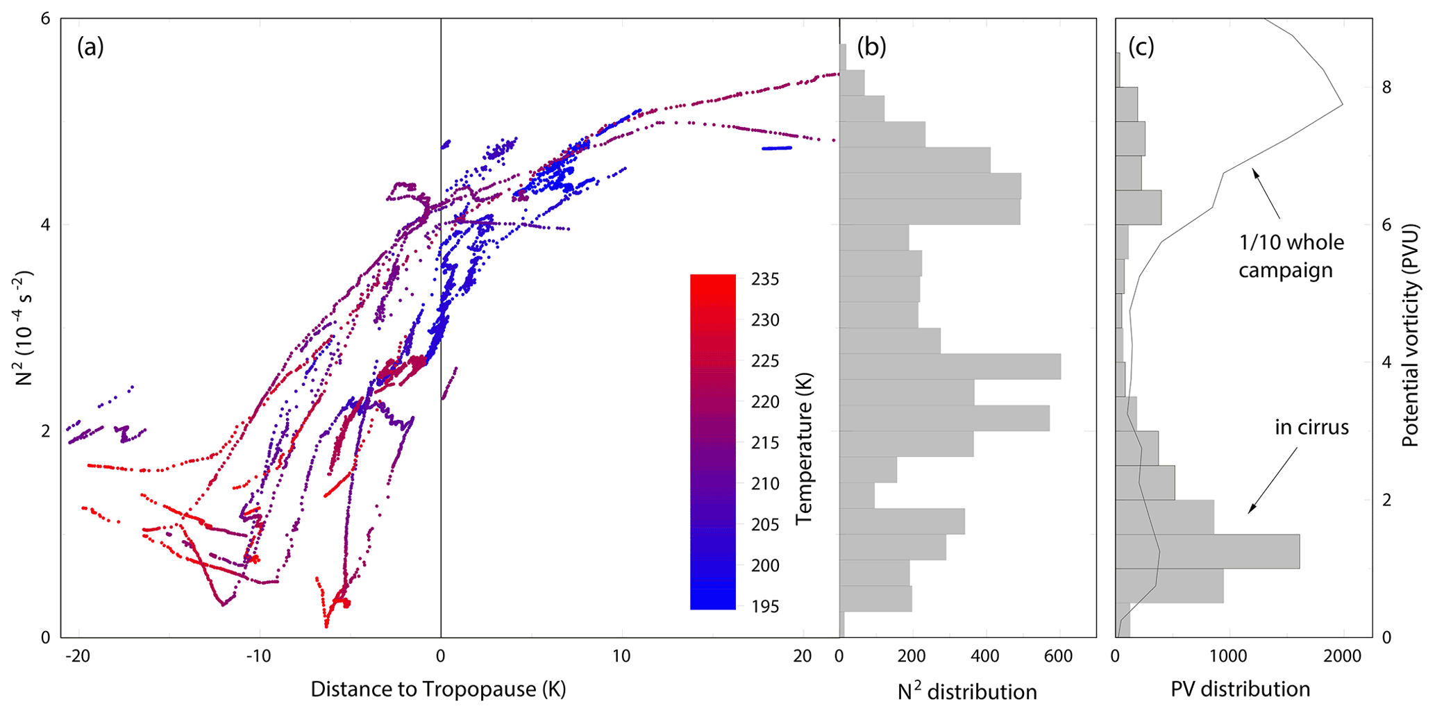
Figure 4 Statistics on the distribution of cirrus sampling below 235 K during POLSTRACC at high latitudes north of 60^∘ N. (a) Distribution over distance to tropopause (given in kelvin, K, of potential temperature) and the squared Brunt–Väisälä frequency (N²). The temperature is indicated using colour coding. (b) The marginal distribution of N². (c) The distribution of potential vorticity. Cirrus sampling is shown using grey bars, and the total campaign flight time (divided by 10) is shown using the black line.

The following sections (Sects. 4 and 5) focus on one subclass of IWC measurements that represent complete vertical profiles of cirrus clouds at the tropopause, seen as the line-forming dots of data in Fig. 4a.

4 Complete profiles of cirrus at the high-latitude tropopause

In order to investigate the radiative impact of cirrus at the tropopause on the profile of temperature and stability, it is necessary to include the complete profile of the respective cloud in the analysis. The POLSTRACC IWC dataset has been filtered to this end, and a selection of eight events was found that displayed the required profiles. These events are listed in Table 1. There are some caveats towards the use of the respective cloud profiles. First, very low IWC values at or below about 10 ppmv are below the associated water vapour concentrations. Although thin cirrus clouds are common in the Arctic (e.g. Hong and Liu, 2015), this complicates the distinction of the precise cloud impact in face of the surrounding atmosphere. Second, some profiles are interrupted by short periods of horizontal flight, extending the time between the cloud bottom and top crossing to well above 10 min. This exacerbates the uncertainty with respect to how well the measurements actually correspond to a real vertical cloud profile. Third, the midlatitude profiles south of 60^∘ N (Germany, Denmark and southern Sweden) are of lesser interest for this study.

Table 1 List of complete cirrus profiles sampled during the POLSTRACC aircraft campaign. The given latitude is an average value for the profile. The acronyms ML and HL are used to categorise the profiles as middle- or high-latitude profiles respectively. z denotes the vertical span, T is the temperature range and the maximum IWC (in molar mixing ratio and in mass concentration) is read from the WARAN measurements. The ice water path (IWP) is calculated by integrating the IWC measurements over the whole profile.

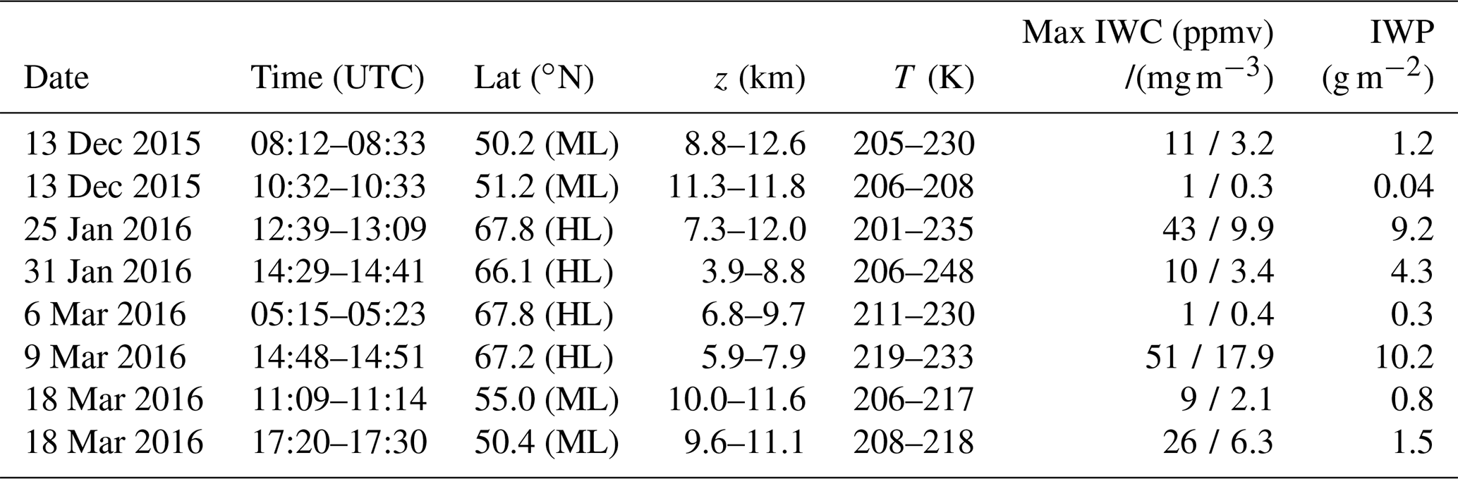
Following these criteria, the profiles on 25 January and 9 March 2016 are the best candidates for the present study. The January profile still includes two horizontal sections with an accumulated duration of 18 min, which equals about 230 km in distance.

Focusing on these two profiles, Fig. 5a and c display respective time–altitude cross sections (curtains). The cirrus profiles are marked by the thicker section of the shown flight paths in orange. The background shading displays the squared Brunt–Väisälä frequency N² from the ECMWF reanalysis as an indicator of the vertical static stability of the atmosphere. The troposphere and stratosphere can be clearly distinguished by dark blue colours and greenish/yellow tones respectively. Tropospheric enhancements with N² up to 4.0 s⁻² in the boundary layer and at 5 km altitude are identifiable. The strongest N² enhancement is found directly above the thermal tropopause (cyan line, representing the WMO definition), marking a pronounced tropopause inversion layer in both cases, despite very different tropopause altitudes. The extended vertical profiles of the reanalysis data show different patterns in both profiles: on 25 January, the stratospheric profile features a fine-scaled structure of static stability that trigger multiple thermal tropopause identifications (cyan lines); in contrast, on 9 March, one broad stratospheric inversion above 13 km can be seen. Both of these observations are not uncommon in regions influenced by orographic gravity waves and in the vicinity of the jet. Missing N² data at low altitudes are due to the orographic cutoff of the reanalysis data above terrain in Scandinavia or Greenland.

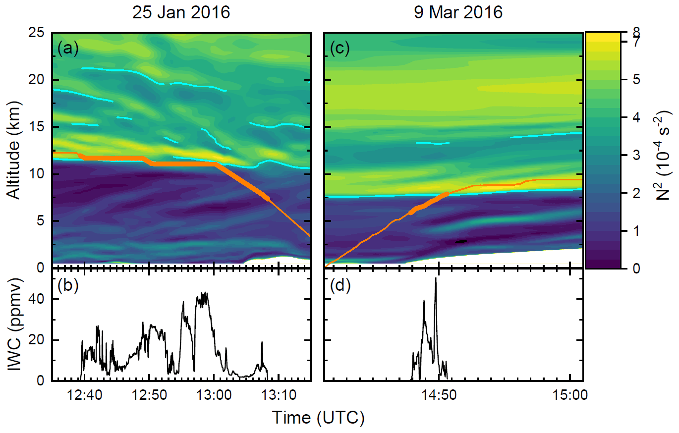
Figure 5 Time series of the cirrus cloud profiles on 25 January and 9 March 2016. In panels (a) and (c), the orange line indicates the aircraft flight path. The thicker section highlights the location of the cloud profile. The background shading displays a vertical cross section of the squared Brunt–Väisälä frequency (N²) from ECMWF reanalysis data interpolated along the flight track. Cyan lines indicate thermal tropopause altitudes according to the WMO definition. Panels (b) and (d) show time series of IWC measurements from the WARAN instrument.

Figure 5b and d contain the in situ IWC measurements from the WARAN instrument, where the time series are aligned with the curtain plots above. On 25 January, the measurements show a considerable variability in the horizontal flight sections, reflecting the overall patchy atmospheric structure. In contrast, the descent towards the end of the profile is characterised by an IWC below 4 ppmv before an enhanced IWC is again observed at the cloud bottom below 8.4 km. On 9 March, the profile exhibits an almost symmetrical double-peaked structure of the IWC distribution inside the cloud. In both cases, the IWC varies frequently by up to 1 order of magnitude. From these slant profiles, we derive vertical IWC profiles for the later sections just by stacking the measurements vertically, neglecting any horizontal inhomogeneity in the clouds. Horizontal flight path sections are condensed into one mean IWC value. Although this no longer represents the actual whole (but unknown) three-dimensional IWC distribution inside the cloud, we still deem these artificial one-dimensional profiles to be realistic. Especially in the critical 25 January case, a very similar profile would result if we only considered the last section of the flight path that contains the majority of the vertical coverage.

We note that possible lower-level clouds might exist below the observed cirrus or also along ground-reaching flight paths. Beyond possible visual identification, such clouds were excluded from sampling (via inlet flow cutoff) during the POLSTRACC campaign to avoid impairment of the targeted measurements of low concentrations of water vapour and cloud water in the upper troposphere and above.

5 Radiative transfer calculations

Radiative transfer calculations focus on the ice clouds that have been probed on 25 January and 9 March 2016. Both days show significant differences in the shape of the IWC(z) and in the geometrical thickness of the ice cloud (Fig. 6). In particular, the IWC(z) profiles reveal vertical fine structures.

This section describes the radiative transfer model, its input and treated radiation parameters. It is shown how the specific properties of the measured IWC(z) profiles affect irradiances, the radiative forcing and heating rate profiles. The radiative effects of the detected IWC fine structures are discussed via comparison to the results that would emerge for IWC profiles with vertically coarser resolutions. The mentioned uncertainty of the IWC measurements, which is likely an underestimation, is addressed by repeated calculations using the IWC profiles multiplied by 5.

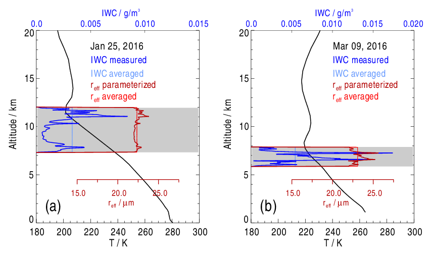
Figure 6 Vertical profiles of the measured ice water content (IWC, dark blue) on (a) 25 January and (b) 9 March 2016 and the effective radius (r_eff, dark red) derived from a parameterisation after Liou et al. (2008) describing r_eff as a function of the IWC. Vertical averages of the IWC and r_eff are indicated using light blue and light red lines respectively. Dark lines show the temperature profiles, and grey shading illustrates the total vertical extent of the measured ice clouds.

5.1 Methods

5.1.1 Radiative transfer model and input parameters

Radiative transfer calculations are based on the uvspec routine from the libRadtran software package (Mayer and Kylling, 2005). The one-dimensional six-stream radiative transfer solver DISORT (DIScrete Ordinate Radiative Transfer) was used to provide static profiles of irradiances and heating rates in the short-wave (SW = 0.24–5.0 µm) and the long-wave (LW = 2.5–100 µm) spectral range. Figure 6 shows IWC profiles measured on 25 January and on 9 March 2016 along with the temperature profiles serving as input. Apart from the IWC, radiative transfer calculations need the effective radius (r_eff). While the IWC is based on in situ measurements, assumptions are made for r_eff. The vertical r_eff(z) profiles have been generated using a parameterisation after Liou et al. (2008) that describes r_eff as a function of the IWC by a polynomial fit of observed data. The data were collected at Arctic latitudes during the Department of Energy (DOE) Atmospheric Radiation Measurement (ARM) Mixed-Phase Arctic Cloud Experiment (M-PACE) at the ARM North Slope of Alaska site in autumn 2004. The effective radii (r_eff) values very probably do not exactly correspond to those present in the ice clouds measured during POLSTRACC, but this way their values may at least be realistically limited.

According to Liou et al. (2008), the dependence of r_eff on the IWC is only weak for Arctic ice clouds and for IWC > 0.0015 g m⁻³. Consequently, Fig. 6 shows relatively small altitude-dependent variations in the r_eff and, similarly, r_eff changes by less than a factor of 2 with the IWC multiplied by 5. Thus, the vertical profile of the ice cloud optical thickness is only highly correlated with the profile of the IWC itself. For IWC < 0.0015 g m⁻³, values of the polynomial fit have been linearly extrapolated to avoid an unrealistic increase in r_eff.

The translation of the IWC and r_eff into the optical properties follows Baum et al. (2005, 2007). Due to the lack of in situ measurements of ice crystal habits during POLSTRACC, the uvspec setting of a general habit mixture (GHM) is taken. The GHM assumes size-dependent fractions of different habits including, for example, pristine crystals like droxtals, columns and plates; bullet rosettes; and aggregates of columns and plates. Under these assumptions the optical thickness of the ice cloud on 25 January 2016 results in τ_0.55 µm = 0.65, and it results in τ_0.55 µm = 0.68 for the ice cloud on 9 March 2016, which is moderately opaque (e.g. Kienast-Sjögren et al., 2016). Horizontally homogeneous model clouds are resolved vertically into 72 layers in order to adequately represent the measured IWC fine structures.

Concerning the reflection properties of the lower boundary, surface types typical of Arctic regions are considered: a snow-/ice-free ocean, a snow-covered surface and one land surface assumed to represent a mix of snow-covered and snow-free areas. In principal, the reflection properties of these surface types are highly variable in time and space and depend on various parameters. The reflection of the ocean, for example, is affected by the surface wind speed and by the type and concentration of existing hydrosols. The reflection properties of snow depend on the grain size of the snow, its age and the degree of pollution. For the sake of simplification, although the term albedo is used in the following, the lower boundary condition of the model atmosphere is described by a spectrally constant and isotropic bidirectional reflection distribution function (BRDF); this function depends on the solar zenith angle (sza) in the case of the ocean and is independent of the sza for snow and the mixed surface. The BRDF is a pure property of the surface and is not affected by atmospheric conditions.

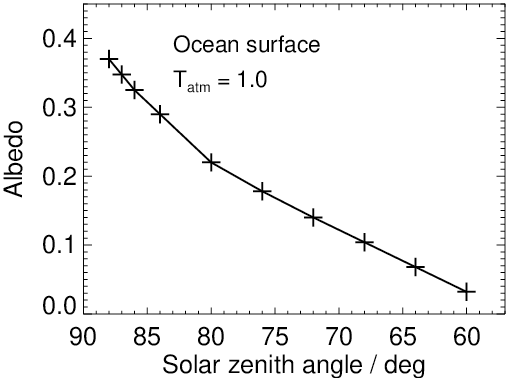
Simplifications are made for numerical simulations. In case of the ocean, a broadband albedo following the measurements of Payne (1972) is used that depends on the sza and represents a mean surface roughness at a wind speed of 7.5 kn (3.9 m s⁻¹). The ocean albedo increases significantly for large sza values. For this study, data corresponding to the curve in Fig. 7 are used. As an approximation, the snow surface is represented by a constant broadband albedo of α_snow 1=0.60 and α_snow 2=0.85, corresponding to old and fresh snow respectively (e.g. Gardner and Sharp, 2010). As the variation in the snow albedo is less pronounced for sza ≥ 60^∘ compared with the ocean albedo, sza-dependence is not taken into account. Furthermore, to estimate the albedo effects of Arctic land surface consisting of different components, such as a mixture of snow and snow-free (rocky) areas, a constant value α_mix=0.30 is used. In the LW range, according to Wilber et al. (1999), a broadband emissivity of ε=0.99 is assumed for the ocean and mixed surface, and ε=1.0 is assumed for snow surfaces.

Figure 7 Broadband albedo at the ocean surface as a function of solar zenith angle after Payne (1972) for an atmospheric transmission of τ_atm=1.0. These values have been used as input for the radiative transfer model.

For aerosol, a uvspec setting is selected that describes a standard maritime haze in the lower 2 km in the winter season. The vertical profiles of the meteorological parameters and the trace gases are described in the following section.

5.1.2 Meteorological data and trace gases

For the one-dimensional radiative transfer calculations, a complete profile of temperature and radiatively relevant species in the troposphere and stratosphere is required. Therefore, we use data from the European Centre for Medium-Range Weather Forecasts (ECMWF) Integrated Forecasting System (IFS) analysis product. Distributions of methane (CH₄), nitrogen monoxide (NO) and nitrogen dioxide (NO₂) are taken from the Copernicus Atmospheric Monitoring Service (CAMS). The ozone (O₃) distribution is taken from the Global and regional Earth-system Monitoring using Satellite and in situ data (GEMS). High-resolution hourly data on 137 model levels are provided for the meteorological quantities (IFS) including specific humidity (3-hourly and 60 levels for CAMS and GEMS). The model data are interpolated in space and time along the flight paths of the HALO aircraft during the POLSTRACC campaign.

In situ values of meteorological quantities like atmospheric pressure and temperature as well as geolocation are provided by the Basic HALO Measurement And Sensor System (BAHAMAS) at a 1 Hz frequency (Giez et al., 2017). The BAHAMAS temperature and humidity data and in situ-measured ozone are only used for comparison in order to assess the consistency of the model with the in situ data during the relevant flight sections. Temperature is captured quite well by the model, with a slight tendency to underestimate the values by up to 2 K. The vertical structure in (slant) profiles is consistent; in particular, the height of the thermal tropopause from both sources coincides. Specific humidity in the vicinity of the IWC measurements (i.e. in neighbouring cloud-free sections) is found to agree within about 5 % and lacks a systematic bias. This also translates into a good representation of specific humidity (for context, see e.g. Kaufmann et al., 2018). The GEMS ozone product is consistent with the in situ measurements from the onboard Fast and Accurate In Situ Ozone Instrument (FAIRO) (Zahn et al., 2012) near the surface and, for the most part, in the stratosphere. In the regime above 500 ppbv O₃, the model does not capture the small-scale variability in the observations, with typical deviations of 15 % to 20 %. Due to the overall satisfactory agreement, model and in situ data are not merged for single atmospheric parameters to avoid possible edge artefacts. Instead, we use the model data for the whole column for all quantities except for the IWC.

5.1.3 Radiative quantities

With a view to the following sections, the definitions of five radiative quantities are given. A basic model output is the upward- and downward-directed irradiance (F_up,Δλ and F_down,Δλ respectively) at each model layer. These irradiances are integrated over a wavelength interval Δλ (here over the SW and LW range) and are given in watts per square metre (W m⁻²). The balance of incoming and outgoing irradiance at each model layer is defined as follows:

$$\begin{array}{}\text{(4)}& F_{\mathrm{\Delta }\mathit{\lambda }}=F_{\mathrm{down},\mathrm{\Delta }\mathit{\lambda }}-F_{\mathrm{up},\mathrm{\Delta }\mathit{\lambda }}.\end{array}$$

Balancing the irradiances F_Δλ over the SW and LW spectral intervals gives the net radiation budget or net irradiance (in W m⁻²), hereinafter referred to as F_net:

$$\begin{array}{}\text{(5)}& F_{\mathrm{net}}=F_{\mathrm{SW}}+F_{\mathrm{LW}}.\end{array}$$

The net forcing RF_net (in W m⁻²) is defined as the difference of F_net calculated for the atmosphere with an embedded ice cloud minus F_net for the cloud-free atmosphere:

$$\begin{array}{}\text{(6)}& {\mathrm{RF}}_{\mathrm{net}}=F_{\mathrm{net},\mathrm{ice}\mathrm{cloud}}-F_{\mathrm{net},\mathrm{cloud}\text{-}\mathrm{free}}.\end{array}$$

The heating rate H_Δλ integrated over the wavelength interval Δλ describes the temperature change in a model layer (in K d⁻¹, kelvin per day) and is defined as follows:

$$\begin{array}{}\text{(7)}& H_{\mathrm{\Delta }\mathit{\lambda }}=-\mathrm{1}/\left({\mathit{\rho }}_{\mathrm{air}}{c}_p\right)\cdot \partial F_{\mathrm{\Delta }\mathit{\lambda }}/\partial z.\end{array}$$

Here, ρ_air denotes the air density, c_p is the specific heat capacity of air at constant pressure and $\partial F_{\mathrm{\Delta }\mathit{\lambda }}/\partial z$ is the vertical divergence of the irradiance F_Δλ. Balancing H_Δλ over the SW and LW spectral interval gives the net heating rate (in K d⁻¹), hereinafter referred to as H_net:

$$\begin{array}{}\text{(8)}& H_{\mathrm{net}}=H_{\mathrm{SW}}+H_{\mathrm{LW}}.\end{array}$$

5.2 Results

5.2.1 TOA net irradiances

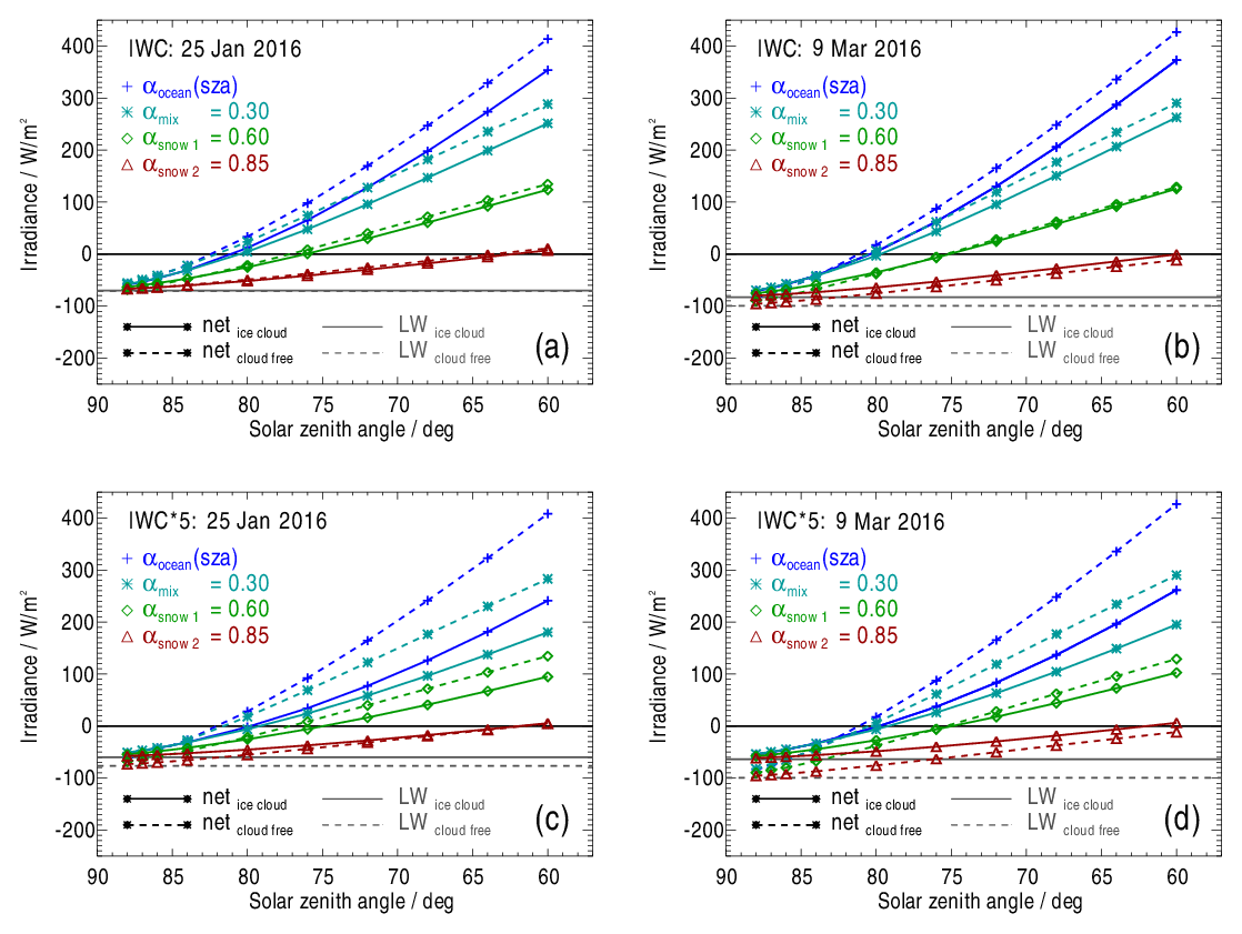
Net irradiances at the TOA (F_net,TOA) as a function of the sza based on IWC profiles measured on 25 January and on 9 March 2016 are shown in Fig. 8. Dashed curves result for the cloud-free atmosphere. Solar zenith angles in the range of 88^∘ ≥ sza ≥ 60^∘ occur at Arctic latitudes north of 66^∘ N within the period from 10 September to 31 March. Horizontal grey lines calculated with ε=1.0 additionally show the LW component of the irradiance (F_LW,TOA). The SW component (F_SW,TOA) is the difference between the curves for F_net,TOA and F_LW,TOA. Figures 8a and b compare F_net,TOA over an ice-free ocean and over surfaces assumed to be covered with aged snow (α_snow 1=0.60) and fresh snow (α_snow 2=0.85). The curve for the albedo α_mix=0.30 is, as mentioned, intended to give an estimate of F_net,TOA for land surfaces with partial snow cover.

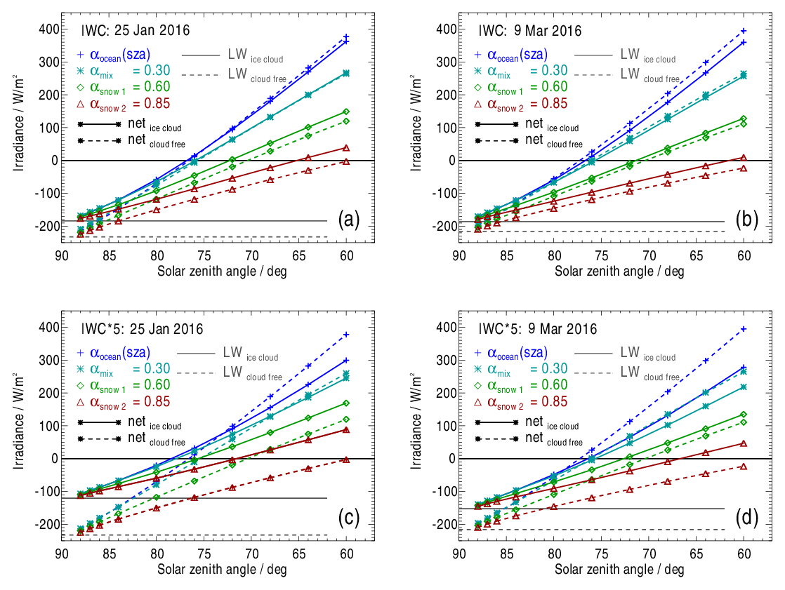
Figure 8 (a) Irradiance at the top of the atmosphere on 25 January 2016 as a function of solar zenith angle over an ice-free ocean, over snow-covered surfaces and over a mixed surface with albedo values as indicated. Panel (b) is the same as panel (a) but for the atmosphere on 9 March 2016. Solid curves show the atmosphere with an embedded ice cloud, whereas dashed curves show a cloud-free atmosphere. Panels (c) and (d) are the same as panels (a) and (b) respectively but for ice clouds with higher optical thicknesses obtained by multiplying the measured profile IWC(z) by a factor of 5. Horizontal grey lines, valid for ε=1.0, indicate the LW component of the irradiance.

Note that, in order to examine the diurnal course of net irradiances for selected geographical locations and days from Fig. 8 (and following figures), the sza simply has to be determined as a function of latitude, longitude, day and daytime. If the local minimum sza is known, the possible irradiance range lies to the left of this sza.

For all curves in Fig. 8, F_net,TOA is minimal at the highest sza and increases with decreasing sza. In other words, with increasing sza, F_net,TOA converges to the long-wave component F_LW,TOA (grey lines).

For a better understanding of sza-dependent irradiances in the short-wave range (F_SW), the following should be noted: with increasing sza, the light paths through the atmosphere become longer. As a consequence, the absolute value of the contribution of the downward-directed irradiance F_SW,down to F_net,down decreases in all layers within the atmosphere. The proportion of the direct component $F_{\mathrm{SW},\mathrm{down},\mathrm{dir}}$ in each atmospheric layer depends on the optical thickness of the atmosphere between this layer and the TOA. Within ice clouds, a large part of $F_{\mathrm{SW},\mathrm{down},\mathrm{dir}}$ is scattered in the forward direction by the ice crystals, but the proportion of direct radiation at the cloud base nevertheless decreases in favour of the diffuse component $F_{\mathrm{SW},\mathrm{down},\mathrm{diff}}$ with increasing sza. For example, on 25 January 2016 and at sza = 64^∘, the proportion of $F_{\mathrm{SW},\mathrm{down},\mathrm{dir}}$ transmitted through the cloud is about 25 % and that of diffuse radiation is, correspondingly, 75 %. For sza = 88^∘, $F_{\mathrm{SW},\mathrm{down},\mathrm{dir}}$ is negligible. At the cloud top, about 26 % of the incident solar irradiance F_SW is reflected at sza = 64^∘, whereas 66 % is reflected at sza = 88^∘. At cloud top, the absolute values of upward-directed irradiances F_SW,up strongly depend on the surface albedo and are highly correlated with F_net,TOA.

Although the difference between F_net,TOA over the ocean and F_net,TOA over the snow surfaces is relatively small (e.g. about 10 W m⁻² for α_ocean=0.37 and α_snow=0.85) at the maximum sza = 88^∘, the curves diverge quickly with decreasing sza (Fig. 8a, b, c, d). The reason for this is that, in the case of atmospheres containing semi-transparent ice clouds or under cloud-free conditions, the contribution of the (positive) F_SW,TOA increases with decreasing surface albedo and with decreasing sza. This effect is further enhanced by differences between the sza-dependent ocean albedo and the constant snow albedo which increase with decreasing sza. As a consequence, the transition from negative to positive values of F_net,TOA, equivalent to a change from a loss to a gain in radiative energy, occurs at a greater sza over the ocean than over aged snow (α_snow 1=0.60) or fresh snow (α_snow 2=0.85). Furthermore, over snow surfaces, the transition from a negative to a positive F_net,TOA is shifted towards a higher sza when compared with results for a cloud-free atmosphere.

In case of the mixed surface (α_mix=0.30), the differences of F_net,TOA between the cloud-free atmosphere and the atmosphere containing an ice cloud are smallest for about sza < 82^∘ (Fig. 8a). This is a constellation where the specific ice cloud properties result in a negligible net radiative forcing RF_net (Eq. 6).

Comparing the curves of F_net,TOA in Fig. 8a and b, their behaviour as a function of sza and surface albedo is qualitatively the same. Differences between cloudy and cloud-free atmospheres, resulting in the radiative forcing (RF_net), are further discussed in Sect. 5.2.3.

The extent to which higher optical thicknesses of the ice clouds affect F_net,TOA was also investigated. For this purpose, measured profiles of IWC(z) were multiplied by a factor of 5, with r_eff being adjusted according to the parameterisation of Liou et al. (2008) in each layer. Higher values of IWC(z) result in optical thicknesses of τ_0.55 µm=2.94 and τ_0.55 µm=2.85 for 25 January and 9 March respectively. In the SW, higher optical thicknesses of the ice clouds lead to a larger contribution of the upward-directed reflected radiation to $F_{\mathrm{net},\mathrm{TOA},\mathrm{SW}}$. At the same time, increased optical thicknesses of ice clouds increase the cloud LW effect, i.e. rendering more surface-emitted LW radiation to be absorbed by ice clouds and, hence, causing $F_{\mathrm{net},\mathrm{LW},\mathrm{TOA}}$ to be less negative (Fig. 8c and d vs. Fig. 8a and  b). One net effect is an overall shift in F_net,TOA towards higher values, which is especially noticeable at a large sza, where SW effects are increasingly negligible. For example, F_net,TOA is increased by about 62 W m⁻² on 25 January and by about 32 W m⁻² on 9 March at sza = 88^∘.

Figure 9 The same as Fig. 8 but for irradiance at the bottom of the atmosphere (surface).

5.2.2 Surface net irradiances

Figure 9 presents net irradiances at the surface (or bottom of the atmosphere) F_net,BOA. The effect of various surface albedo values on the relative course of the curves with respect to each other corresponds to that in Fig. 8. However, in comparison to F_net,TOA (Fig. 8), the decrease in F_net,BOA with increasing sza is less pronounced. The reason for this is the generally reduced LW radiation emission from the surface (F_LW,BOA), as the values at sza = 88^∘ show. F_LW,BOA is the limiting factor for F_net,BOA. At the other end of the x axis, at small sza values, the curves of F_net,BOA (Fig. 9) and F_net,TOA (Fig. 8) tend to converge for the same albedo values, which is a consequence of increasing forward scattering of incoming SW radiation at the ice crystals. Generally, with decreasing sza, an increasing short-wave component F_SW,BOA increases F_net,BOA, which is an effect that becomes stronger moving toward smaller surface albedo values. For α_snow 2=0.85, the difference between the downward- and upward-directed components of F_SW,BOA is minimal, leading to a weak dependence of F_net,BOA on sza (Fig. 9a, b, c, d). As can also be seen from Fig. 9, the ice cloud lowers the positive F_net,BOA at the dark ocean surface within a wide range of sza values when compared with the cloud-free atmosphere. The reason for this is a dominating shadowing effect of the ice clouds, i.e. the downward-directed F_SW,BOA is reduced more strongly than the surface LW emission F_LW,BOA changes (see grey solid and dashed lines in Fig. 9). Over a bright snow surface with α_snow 2=0.85, SW contributions to F_net,BOA become smaller, leading to correspondingly smaller changes in F_net,BOA. In most cases, the curves representing the cloud-free atmosphere are even below those of the cloudy atmosphere. F_net,BOA based on the IWC multiplied by 5 is shown in Fig. 9c and d.

5.2.3 Radiative forcing

Net radiative forcings at the TOA (RF_net,TOA), as defined by Eq. (6), are displayed as a function of sza for 25 January 2016 and 9 March 2016 in Figs. 10a–d. Over bright snow surfaces, RF_net,TOA is positive on both days within the entire range of 88^∘ ≥ sza ≥ 60^∘.

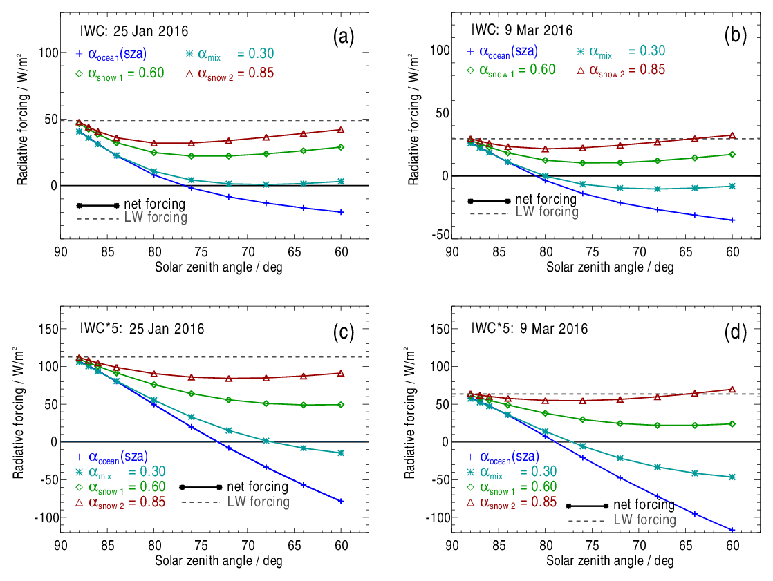
Figure 10 Radiative forcing at the top of the atmosphere as a function of the solar zenith angle on (a) 25 January 2016 and on (b) 9 March 2016 for different surface albedo assumptions as indicated. Panels (c) and (d) are the same as panels (a) and (b) respectively but for ice clouds with higher optical thicknesses obtained by multiplying the measured profile IWC(z) by a factor of 5. Horizontal dashed lines, valid for ε=1.0, indicate the LW component of the forcing.

At sza = 88^∘, the net forcing is mainly determined by the LW forcing, resulting in an energy gain in the system. With a decreasing sza in the range of about 88^∘ > sza > 70^∘, an ice cloud over snow (and partly over the mixed surface) increases the amount of reflected SW radiation, leading to a reduction in the atmospheric energy gain. For sza < 70^∘, the amount of reflected SW radiation decreases due to the pronounced forward scattering of ice crystals, herewith causing an increase in RF_net,TOA.

Over the ocean, positive RF_net,TOA values result for sza > 68^∘ on 25 January 2016 and for sza > 78^∘ on 9 February 2016. For smaller sza values, RF_net,TOA even turns into the negative range. One reason for a negative RF_net,TOA is that the ocean albedo is relatively high at a large sza, but it decreases significantly with decreasing sza (Fig. 7). The smaller the ocean albedo becomes with decreasing sza, the larger the relative contribution of outgoing SW radiation that reduces RF_net,TOA. In general, it can be said that the sign of RF_SW,TOA is predominantly determined by whether the ice cloud albedo is greater or smaller than the surface albedo. Furthermore, ice cloud layers emit at higher temperatures on 9 March 2016 with the consequence that the LW component of the radiative forcing is about 15–20 W m⁻² smaller than on 25 January 2016. All curves are affected; over the ocean, this means that the transition of RF_net,TOA into negative values is shifted towards a larger sza (Fig. 10a, b). Curves for RF_net,TOA with the IWC multiplied by 5 are displayed in Fig. 10c and d. Their greater spread is a consequence of increased ice cloud optical thicknesses.

5.2.4 IWC fine structures

As mentioned, IWC profiles measured during the POLSTRACC campaign show vertical fine structures (Fig. 6a, b). It is investigated how such structures affect the profiles of the net irradiances F_net(z) and heating rates H(z). As a reference, additional radiative transfer calculations have been carried out for synthetic ice clouds with a vertically constant IWC profile, IWC(z)_const. In a second step, IWC profiles with different vertical resolutions are used as a reference. All synthetic IWC profiles together with the assigned profiles of the effective radius r_eff(z,IWC(z)) after Liou et al. (2008) are designed in such a way that the optical thickness is the same as for IWC(z)_meas. Note that the profiles of the temperature affecting the LW irradiance profiles are displayed in Fig. 6.

Figure 11a, e, i and m compare SW and LW irradiance profiles, F_SW(z) and F_LW(z), calculated for the IWC(z)_meas and IWC(z)_const profiles. Altitude-dependent differences in F_SW(z) and F_LW(z) (solid and dashed lines) follow the corresponding difference between IWC(z)_meas and IWC(z)_const. Note that, apart from the influence of trace gases and aerosols and in view of relatively weak variability in the profiles of r_eff(z, IWC(z)) (Fig. 6), the LW thermal emission of a layer is proportional to the ice water content and, thus, proportional to the cloud optical thickness of the layer. In addition, the LW emission depends on the temperature distribution within the ice cloud layer. At the large solar zenith angle sza = 88^∘, LW radiation dominates the altitude-dependent changes in F_LW(z) (Fig. 11a, i).

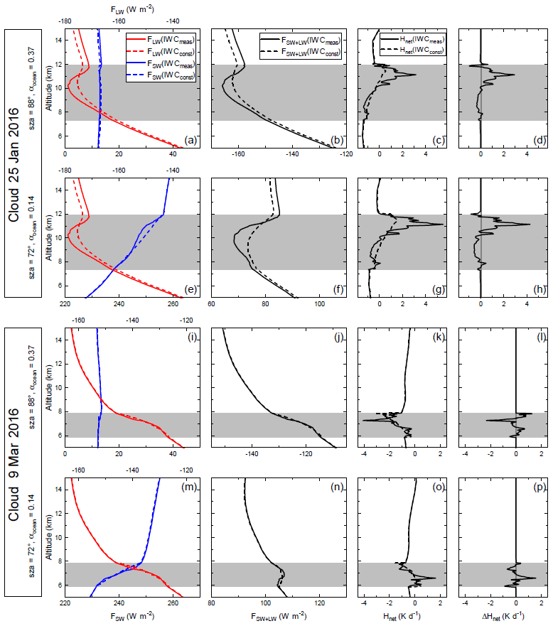
Figure 11 Irradiance profiles of measured (solid) and constant (dashed) IWC profiles for selected values of solar zenith angle and albedo as indicated. Panels (a), (e), (i) and (m) show the LW (red, top axis scale) and SW (blue, bottom axis scale) irradiances. The top axis is shown using negative numbers because F_LW is directed upward. Panels (b), (f), (j) and (n) depict the net irradiances. All irradiance scales span a range of 50 W m⁻², albeit at different absolute positions. Panels (c), (g), (k) and (o) show the net heating rate profiles of the measured and the constant IWC profiles. Panels (d), (h), (l) and (p) outline the difference between the net heating rate profiles of the measured and the constant IWC profiles.

On 25 January 2016, LW irradiances at the cloud top (F_LW,TOC) are smaller for the measured profile IWC(z)_meas compared with F_LW,TOC which is related to IWC(z)_const (Fig. 11a). The reason for this is a smaller LW emission from the IWC maximum near the cloud top due to relatively cold temperatures in combination with an increased optical thickness here. Below the upper IWC peak, F_LW calculated for IWC(z)_meas is larger than for IWC(z)_const because the upward-directed emissions from the surface and from the IWC maximum near the cloud base are balanced by smaller downward-directed emissions from colder layers above. Major differences between irradiances for the IWC(z)_meas and IWC(z)_const are confined to the layers within the cloud and reach up to about 5 W m⁻². Thus, on 25 January 2016, it is the combination of the vertical inhomogeneity of the IWC profile (two different maxima) and the geometrical thickness of the entire ice cloud associated with larger vertical temperature differences that causes pronounced altitude-dependent LW irradiance differences. The ice cloud causes irradiance differences in the order of a few watts per square metre which penetrate up to the TOA (Table 2).

On 9 March 2016, the geometrical thickness of the ice cloud is reduced showing two closely spaced maxima in the middle of the IWC profile. The overall shape is more symmetric than on 25 January 2016 (Fig. 6b). Switching from the measured to the constant IWC profile does not lead to a stronger weighting of layers emitting LW radiation with significantly different temperatures. As a consequence, LW irradiance differences inside the ice cloud are smaller than on 25 January 2016 (about 2 W m⁻²) and even smaller at the TOA and BOA (Fig. 11i, Table 2).

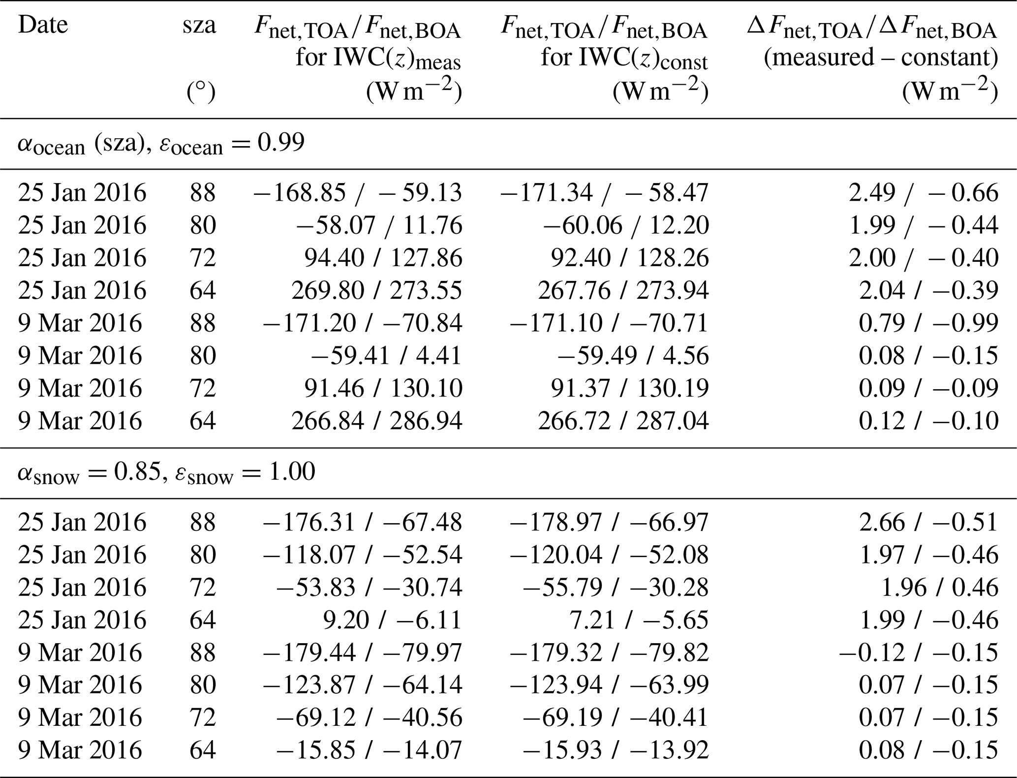
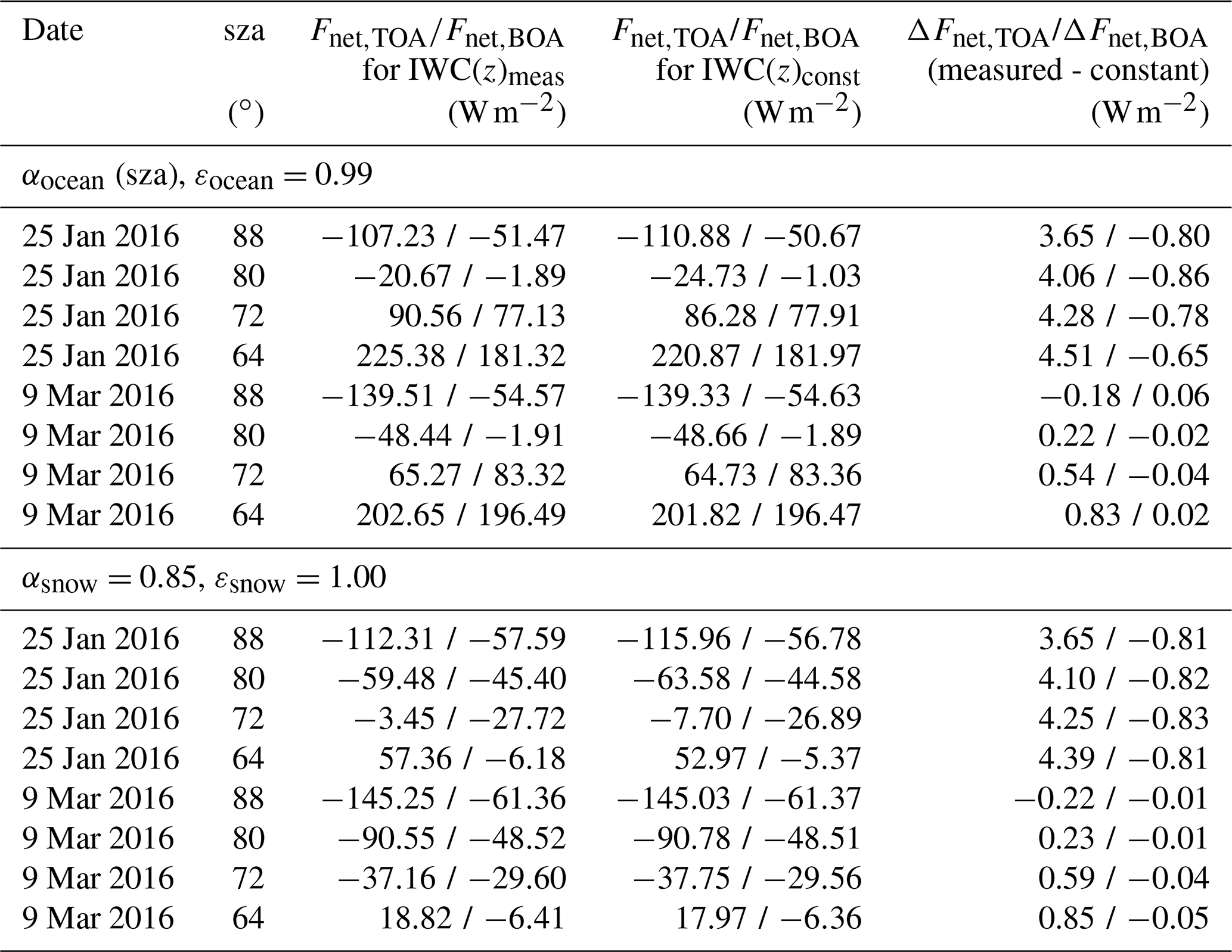
Table 2 Net irradiances at the top of the atmosphere and at the surface (F_net,TOA and F_net,BOA respectively) calculated for measured and vertically constant profiles of the ice water content (IWC(z)_meas and IWC(z)_const respectively). ΔF_net is the difference of F_net(IWC_meas) minus F_net(IWC_const). Results are selected for four solar zenith angle (sza) values and for the days 25 January and 9 March 2016.

A smaller solar zenith angle of sza = 72^∘ increases the contribution of SW radiation significantly (Fig. 11e, m). Irradiance differences due to the influence of differently shaped IWC profiles are mainly a result of scattering processes. SW downward-directed irradiances F_SW(z) calculated for IWC(z)_meas are smaller below the relative IWC maxima. The for this reason is that the cloud optical thickness (and thus the extinction due to scattering) is higher at altitudes of the IWC maxima when compared with values of the constant profile IWC(z)_const at the same altitude (Figs. 6 and 11e, m). On 25 January 2016, the vertically extended maximum of the IWC produces the greatest differences. On 9 March 2016, small enhancements of the downward-directed F_SW(z) result for IWC(z)_meas at the upper edge of the maxima due to multiple-scattering effects (Fig. 11m).

Figure 11b, f, j and n compare profiles of net irradiances F_net(z) balanced over the SW and LW range based on IWC(z)_meas and IWC(z)_const. As is to be expected, F_net(z) reflects that the specific properties of the profile IWC(z)_meas on 25 January 2016 cause the greatest differences to the results obtained for IWC(z)_const. Table 2 contains data of F_net(IWC(z)_meas) and F_net(IWC(z)_const) as well as their differences ΔF_net=F_net(IWC(z)_meas) − F_net(IWC(z)_const) at the TOA and at the BOA. Numbers show that, for the individual day, ΔF_net,TOA and ΔF_net,BOA are of the same order of magnitude independent of the two surface types considered. In most cases, the absolute values of ΔF_net are smaller than 1 W m⁻². An exception is again the results for 25 January 2016 at TOA. The reason for this is already given in Fig. 11a and e, which show that the upward-directed F_LW,TOC calculated for IWC(z)_const at cloud top differs by about 2.5 W m⁻² compared with F_LW,TOC related to IWC(z)_meas. The results obtained with the IWC multiplied by 5 are presented in Table A1.

Vertical profiles of the IWC are not always available at high vertical resolution. In models (e.g. climate models), the vertical resolution of ice clouds near the tropopause is usually in the order of several hundred metres. The effect of different IWC vertical resolutions on F_net,TOA is illustrated in Fig. 12. This shows differences between F_net,TOA based on the IWC measurements on 25 January 2016 and 9 March 2016 and F_net,TOA calculated for IWC profiles resulting from a division of the entire ice cloud into an increasing number of sublayers. Within these sublayers, the IWC is vertically averaged. As shown in Fig. 12, the curves of ΔF_net,TOA converge relatively quickly to zero with the number of sublayers, although this convergence is different for 25 January 2016 and 9 March 2016. The reason for this is again given by the different IWC profiles on both days. On 25 January, a resolution of the ice cloud into 10 sublayers (∼460 m) results in $\mathrm{\Delta }{F}_{\mathrm{net},\mathrm{TOA}}<\mathrm{0.4}\mathrm{W}{\mathrm{m}}^{-\mathrm{2}}$, whereas $\mathrm{\Delta }{F}_{\mathrm{net},\mathrm{TOA}}<\mathrm{0.2}\mathrm{W}{\mathrm{m}}^{-\mathrm{2}}$ is already reached for a resolution into 5 sublayers (∼400 m) on 9 March. This is valid for sza = 88^∘ as well as for sza = 72^∘.

Figure 12 Differences between net irradiances (F_net,TOA) calculated for the measured IWC profile and IWC profiles with different vertical resolution. The x axis shows the number of layers into which the entire ice cloud is divided.

5.2.5 Heating rates

According to Eq. (7), wavelength-integrated net heating rate profiles are proportional to the vertical divergence of the net irradiance $\partial F_{\mathrm{net}}\left(z\right)/\partial z$ and can be read from the profiles shown in Fig. 11b, f, j and n (results in Fig. 11c, g, k and o). $\partial F_{\mathrm{net}}\left(z\right)/\partial z$ is mainly affected by the profile of IWC(z) within the ice cloud; thus, $\partial F_{\mathrm{net}}\left(z\right)/\partial z$ differences due to IWC(z)_meas and IWC(z)_const are particularly pronounced within the ice cloud and are minimal above and below the ice cloud layer. As a consequence, differences in net heating rate profiles ΔH_net(z) associated with IWC(z)_meas and IWC(z)_const occur within the ice cloud on both days (25 January and 9 March 2016) and for both solar zenith angles (sza = 88^∘ and sza = 72^∘) (Fig. 11d, h, l, p). On 25 January 2016, the maximum difference ΔH_net is 4.27 K d⁻¹ at sza = 72^∘, whereas the minimum ΔH_net results in −0.99 K d⁻¹ at sza = 88^∘. On 9 March 2016, the corresponding maximum and minimum values are 1.57 and −2.33 K d⁻¹ respectively. Within the cloud, ΔH_net is in the order of the magnitude of the net heating rate H_net(z), whereas ΔH_net(z) is negligible above and below the cloud.

Figure 11 presents curves that result for an ocean surface as the lower boundary. Comparing heating rate differences $\mathrm{\Delta }{H}_{\mathrm{net}}=H_{\mathrm{net}}\left({\mathrm{IWC}}_{\mathrm{meas}}\right)-H_{\mathrm{net}}\left({\mathrm{IWC}}_{\mathrm{const}}\right)$ over the ocean with those over snow (α_snow 2=0.85) reveals a difference of 0.02 K d⁻¹ (−0.15 K d⁻¹) at the altitude of the maximum ΔH_net for sza = 88^∘ (sza = 72^∘) on 25 January 2016 (not shown). The corresponding change at the minimum ΔH_net results in 0.002 K d⁻¹ (−0.05 K d⁻¹). Furthermore, on 9 March 2016, changes at the maximum and minimum ΔH_net are very small. At the BOA, all changes are in the order of 10⁻⁴ K d⁻¹. Thus, the transition from the ocean surface to a bright snow surface results in small changes in the heating rate profiles, both within and outside the ice cloud.

When multiplying the IWC by 5 (Fig. 13), ΔH_net(z) changes significantly in shape. On 25 January, the maximum is 7.48 K d⁻¹ for sza = 72^∘, and the minimum ΔH_net is −5.21 K d⁻¹ for sza = 88^∘. On 9 March, the maximum and minimum values of ΔH_net(z) are 9.06 and −11.54 K d⁻¹ respectively, which both result from sza = 88^∘. The change in shape or vertical dependency is due to the high optical thicknesses of the clouds and manifests itself mainly in two features: first, the scaling of ΔH_net(z) with z is stronger at lower altitudes than up higher, due to the higher absolute concentration of ice water in the thicker air at lower altitudes; second, the influence of the SW contribution is more limited to the uppermost cloud layers. This leads to a reduced warming impact of the SW regime on the overall heating rate profile, especially in the 9 March case, where the majority of the IWC distribution is more centred in the cloud profile. Nonetheless, ΔH_net still remains negligible above and below the clouds.

Figure 13 The same as Fig. 11d, h, l and p but for ice clouds with higher optical thicknesses as a result of multiplying the entire profile IWC(z) by a factor of 5.

6 Discussion and conclusions

Our radiative transfer simulations for selected profiles of the IWC measured during the POLSTRACC campaign indicate that an ice cloud of extended geometrical thickness and a specific vertically asymmetric fine structure of the IWC change the radiation budget at the TOA compared with the results of a vertically constant IWC profile of equal optical thickness. Effects are significant and, for our cases, in the order of a few watts per square metre (W m⁻²). Fine structures in geometrically thin ice clouds that have a more symmetric IWC profile do not lead to a noticeable modification of the TOA radiation budget when compared to the case of a vertically constant IWC. This is consistent with the results of Feofilov et al. (2015), who performed a statistical analysis of cirrus IWC profiles and their radiative effects from active and passive spaceborne remote sensing products. Similar to our above result, they concluded that the LW effect of a certain profile (at the TOA) is modulated by an “effective radiative layer” with respect to a constant IWC profile, which reflects internal inhomogeneity in the vertical IWC distribution. We show that the uncertainty arising from a possible coarser vertical resolution is reduced to below 20 % for the inhomogeneous IWC profile if layers are thinner than about 500 m. The study by Feofilov et al. (2015) is dominated by low and midlatitude cirrus properties with a higher IWP and optical thickness. In contrast, our analyses are focused on thinner (still opaque) Arctic cirrus clouds that exist in darkness or at high solar zenith angles such that their net radiative forcing may be of alternating sign.

A significant impact on net irradiances at the top and the bottom of the atmosphere is found to originate from the albedo of typical Arctic surface types, such as the open ocean or snow-covered regions, which also implies effects on the radiative forcing. Depending on the solar zenith angle, effects are strong for F_net,TOA and mostly strong or moderate for F_net,BOA but weak for F_net,BOA under conditions of fresh fallen snow. Age and pollution of snow seem important factors in this context. For example, the transition from negative to positive values of the TOA radiation budget, equivalent to a change from a loss to a gain in radiative energy, occurs at greater solar zenith angles over the ocean than, for example, over aged snow (α_snow=0.60). Furthermore, over aged snow, the transition is shifted towards a higher solar zenith angle when compared with results for a cloud-free atmosphere. This means that the presence of cirrus leads to an enhanced gain in radiative energy in the Arctic atmosphere in most cases during autumn to spring as well as over bright surfaces. Therefore, in scenarios with an overall negative trend in surface albedos in the Arctic, the positive radiative forcing effect of cirrus is expected to decrease. This decrease is relevant in view of the Arctic amplification (e.g. Wendisch et al., 2017; Perovich and Polashenski, 2012; Thackeray and Hall, 2019), as it constitutes a possible counteracting effect. Notwithstanding, the (direct) impact on surface net irradiances and, therefore, on surface temperature is much less pronounced.

Instantaneous heating rate profiles of the atmosphere are mainly affected by fine structures of the IWC within the cloud layer and remain negligible below and above the cloud. The effect of different surface albedo values on instantaneous heating rate profiles is only very weak. Depending on the profile of IWC or optical thickness, the heating rate profile can contribute to a strengthening or weakening of a given structure in the temperature profile, especially concerning the cold point of the tropopause, as well as the strength of the above inversion layer. The strong tropospheric lapse rate in some of our observed cloud profiles induces a stabilising radiative effect of the cloud in most of the tropospheric heating rate profile inside the cloud layer, with an overall higher (LW) heating rate at the cloud top (warming) than at the cloud bottom (less warming or cooling). However, first of all, a heating rate profile will trigger cloud internal processes through evaporation or latent heat release that drive vertical motion, modify the temperature gradient and change the microphysical properties of the ice particles.

Concerning a probable underestimation of the IWC in the measurements, we derived that a potentially higher true IWC profile would lead, as can be expected, to a higher warming impact of the cirrus on the TOA radiation budget and would dampen the effect of different surface albedo values. At the same time, the heating rate profiles would be more dominated by the LW contribution due to the strongly enhanced optical thickness. Still, we conclude that our original calculations are of value because many thinner cirrus clouds exist in the Arctic (and were observed) to which our results would apply accordingly, beyond the two cases that we analysed.

7 Outlook

Some aspects of Arctic ice clouds have not been treated in this work, such as the effects of the modification of size and number density by specific cloud formation regimes. Likewise, the effects of different ice crystal habits or habit compositions on SW and LW irradiances, radiative forcings and heating rates were not in the focus of this study. Based on measurements of a subtropical cirrus, studies such as Wendisch et al. (2005) and Wendisch et al. (2007) have shown that irradiances are significantly sensitive to different ice crystal shapes in the SW and LW, depending on solar zenith angle, location above or below the cloud, cirrus optical thickness, and the spectral region within the SW and LW range. For certain constellations, maximum changes in irradiances even reach 26 % in the SW and up to 70 % in the LW. The effects of specific habits (i.e. hexagonal columns, plates, rosettes, aggregates and spheres) are intercompared. As mentioned, radiative transfer calculations in this study have been carried out under the assumption of a general habit mixture (GHM) due to the lack of in situ measurements of ice crystal habits during the POLSTRACC campaign. It cannot be ruled out that different habit mixes occur in the Arctic, in which pristine crystals (e.g. hexagonal plates or columns) play a more dominant role. Nevertheless, we choose the GHM because the assumption that an ice cloud consists of one habit type only also seems unrealistic.

The flight and measurement strategies pose additional sources of uncertainty. Slant pseudo-vertical IWC profiles or, even more so, those with intermediate level flight sections extend horizontally over several 10 to 100 km and likely do not adequately account for lateral inhomogeneity within the cirrus cloud field. This uncertainty might be reduced with higher vertical speed, at the cost of reduced vertical resolution or sensor accuracy, or better quantified by repeated sampling in different directions or co-located satellite observations. Similar studies would also greatly benefit from information on potential lower cloud coverage below the cirrus.

Recent and current observational activities will provide additional data on cloud microphysical properties to better represent real Arctic cirrus in future work, aiming for a closure of the physics of particle-scale processes with the radiation field. In this respect, the in situ measurements of the recent CIRRUS-HL (Cirrus in High Latitudes) mission are very promising. Further useful contributions are expected to come from ongoing and planned campaign activities.

Appendix A

This appendix includes a table similar to Table 2 but showing further results from radiative transfer calculations that were carried out with IWC profiles scaled by a factor of 5, as described in the main text.

Table A1 The same as Table 2 but for ice clouds with higher optical thicknesses as a result of multiplying the entire profile IWC(z) by a factor of 5.