Convective organization and 3D structure of tropical cloud systems deduced from synergistic A-Train observations and machine learning

We are building a 3D description of upper tropospheric (UT) cloud systems in order to study the relation between convection and cirrus anvils. For this purpose we used cloud data from the Atmospheric InfraRed Sounder and the Infrared Atmospheric Sounding Interferometer and atmospheric and surface properties from the meteorological reanalyses ERA-Interim and machine learning techniques. The different artificial neural network models were trained on collocated radar–lidar data from the A-Train in order to add cloud top height, cloud vertical extent and cloud layering, as well as a rain intensity classification to describe the UT cloud systems. The latter has an accuracy of about 65 % to 70 % and allows us to build objects of strong precipitation, used to identify convective organization. This rain intensity classification is more efficient to detect large latent heating than cold cloud temperature. In combination with a cloud system analysis, we found that deeper convection leads to larger heavy rain areas and a larger detrainment, with a slightly smaller thick anvil emissivity. This kind of analysis can be used for a process-oriented evaluation of convective precipitation parameterizations in climate models. Furthermore, we have shown the usefulness of our data to investigate tropical convective organization metrics. A comparison of different tropical convective organization indices and proxies to define convective areas has revealed that all indices show a similar annual cycle in convective organization, in phase with convective core height and anvil detrainment. The geographical patterns and magnitudes in radiative heating rate interannual changes with respect to one specific convective organization index (I_org) for the period 2008 to 2018 are similar to the ones related to the El Niño–Southern Oscillation. However, since the interannual anomalies of the convective organization indices are very small and noisy, it was impossible to find a coherent relationship with those of other tropical mean variables such as surface temperature, thin cirrus area or subsidence area.

1 Introduction

Upper tropospheric (UT) clouds represent about 60 % of the total cloud cover in the deep tropics (e.g. Stubenrauch et al., 2013, 2017). These clouds, when created as anvil outflow from deep convection, often build large systems (e.g. Houze, 2004). The creation and maintenance of these mesoscale convective systems (MCSs) is strongly dependent on the moisture available in the lower troposphere and is influenced by wind shear (e.g. Laing and Fritsch, 2000; Chen et al., 2015; Schiro et al., 2020). Observational and cloud-resolving model (CRM) studies (e.g. Del Genio and Kovari, 200; Posselt et al., 2012) have shown that tropical storm systems over warmer water are denser with more intense precipitation and cover wider areas than those over cooler water. Thin cirrus surround the highest anvils (Protopapadaki et al., 2017), which may be explained by UT humidification originating from deep convection (e.g. Su et al., 2006). Their structure and amount may respond to changing convection induced by climate warming. Organized convection, leading to MCSs and therefore associated to extreme precipitation, is a research subject of high interest, in particular in regard to climate warming, and many results have been published (e.g. Popp and Bony, 2020; Bony et al., 2020; Pendergrass, 2020; Bläckberg and Singh, 2022).

The goal of this article is to present a coherent long-term 3D dataset which describes tropical UT cloud systems and which can be used on the one hand for a process-oriented evaluation of convective parameterizations in climate models and on the other hand for the study of convective organization.

For the study of the relation between cirrus anvils and convection, we coupled horizontal and vertical structure of UT clouds, including precipitation and 3D radiative heating. As single datasets are incomplete, we used their synergy and machine learning (ML) to get a more complete 3D description as well as simultaneous information on precipitation. A cloud system approach makes it possible to link the anvil properties to convection. Furthermore, the horizontal structure of intense rain areas within these cloud systems can be used to derive tropical convective organization indices.

The cross-track scanning Atmospheric Infrared Sounder (AIRS) and the Infrared Atmospheric Sounding Interferometers (IASI), aboard the polar-orbiting Aqua and Metop satellites, provide cloud properties (CIRS, Clouds from IR Sounders; Stubenrauch et al., 2017) with a large instantaneous horizontal coverage. These have been used to reconstruct UT cloud systems (Protopapadaki et al., 2017). The good spectral resolution of IR sounders makes them sensitive to cirrus, down to a visible optical depth of 0.1, during daytime and nighttime. The vertical cloud structure is derived by combined radar–lidar measurements of the CloudSat and CALIPSO missions (Stephens et al., 2018) but only along successive narrow nadir tracks separated by about 2500 km. In order to get a more complete instantaneous picture, required for process studies, Stubenrauch et al. (2021) have demonstrated that the radiative heating rate profiles derived along these nadir tracks (CloudSat FLXHR-lidar; Henderson et al., 2013) can be horizontally extended by artificial neural network (ANN) regression models applied on cloud properties retrieved from AIRS and atmospheric and surface properties from meteorological re-analyses from the European Centre for Medium-range Weather Forecasts (ECMWF). The 15-year time series reveals a connection of the heating by MCSs in the upper and middle troposphere and the (low-level) cloud cooling in the lower atmosphere in the cool regions, with a correlation coefficient equal to 0.72, supporting the hypothesis of an energetic connection between the convective regions and the subsidence regions.

This article presents additional variables expanded to the horizontal coverage of AIRS and IASI by machine learning models, trained with collocated CloudSat-lidar retrievals: cloud top height, cloud vertical extent and cloud layering (above and below the clouds identified by CIRS), as well as a precipitation intensity classification (no, light or heavy).

Apart from the conclusions and outlook given in Sect. 4, the article is divided into two main sections: Sect. 2 describes the data, methods and evaluation; and Sect. 3 highlights scientific results which show the applicability of these newly derived variables.

Section 2 first describes the collocated data, the neural network development as well as an evaluation of the predictions on the collocated data. In addition, it presents the creation of the 3D dataset containing the additional variables (Sect. 2.3) and the cloud system reconstruction (Sect. 2.4). The last subsection (Sect. 2.5) gives a short overview of existing convective organization indices and proxies for defining the convective objects. Section 3 first shows the coherence of these ML-derived properties, in particular the rain intensity classification, using the complete 3D dataset (Sect. 3.1). Then, in combination with a cloud system analysis, Sect. 3.2 presents the MCS properties with respect to their life cycle stage and their convective depth. The last subsection (Sect. 3.3) explores tropical convective organization: we compare different proxies for convection and resulting indices of convective organization, by investigating annual cycle and interannual variability. The latter is small over the considered time period (2008–2018), but we find interesting geographical patterns in changes of radiative heating rate fields in relation to the tropical convective organization.

2 Data, methods and evaluation

Satellite observations have become a major tool to observe our planet. However, they do not provide instantaneous complete views, because passive remote sensing is not able to provide the vertical structure of clouds and active radar–lidar measurements are only available along very narrow nadir tracks. In order to build a complete 3D cloud dataset, we combine the complementary information from passive and active remote sensing, and we train artificial neural networks over these collocated data.

2.1 Collocated AIRS–CloudSat-lidar–ERA-Interim data

The satellite observations used for the training originate from the A-Train constellation (Stephens et al., 2018), with local overpass times around 01:30 and 13:30. As input variables for the ANNs, we use cloud properties retrieved from AIRS measurements by the CIRS (Clouds from IR Sounders) algorithm (Stubenrauch et al., 2017) and coincident atmospheric and surface properties from meteorological reanalyses ERA-Interim (Dee et al., 2011). CIRS cloud types are defined according to cloud pressure (p_cld) and cloud emissivity (ε_cld) from AIRS–CIRS as high-level clouds with p_cld < 440 hPa and further as high opaque with ε_cld > 0.95, cirrus with 0.95 > ε_cld > 0.5 and thin cirrus with 0.5 > ε_cld > 0.05. Mid-level clouds (440 hPa < p_cld < 680 hPa) and low-level clouds (p_cld > 680 hPa) are both separated into two categories: opaque with ε_cld > 0.5 and partly cloudy with ε_cld < 0.5.

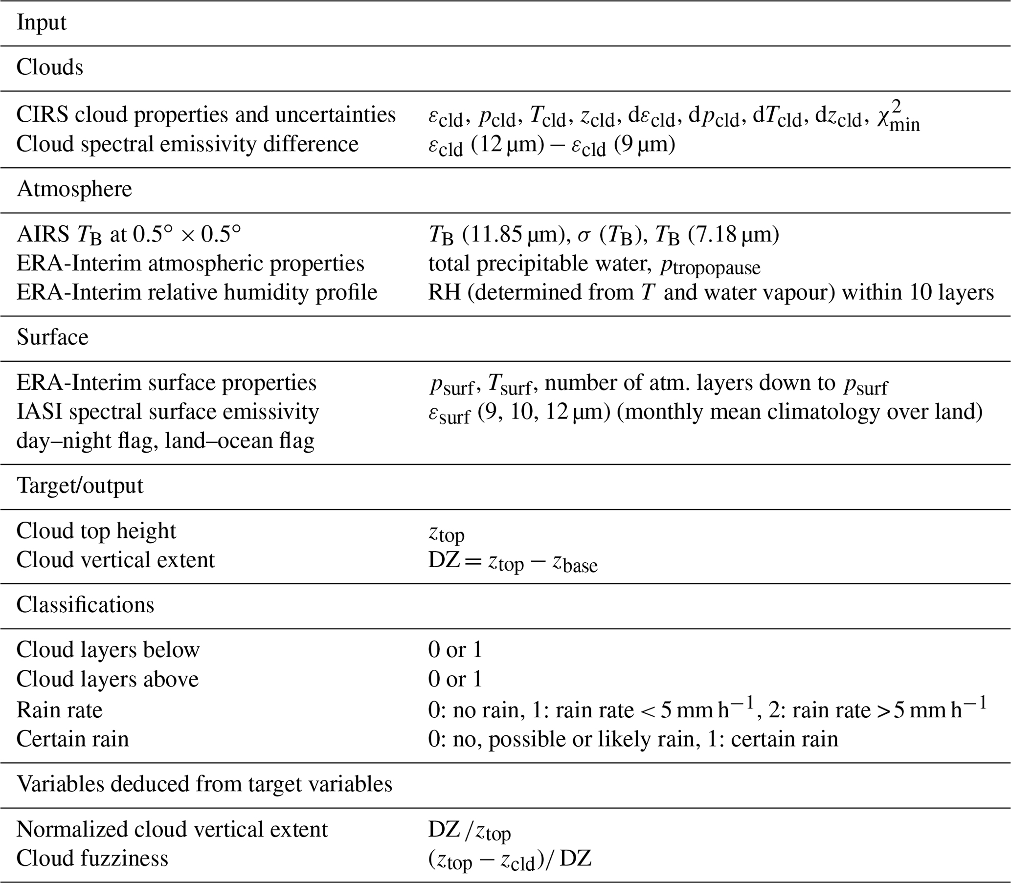
The target variables are products derived from combined radar–lidar measurements from the CloudSat and CALIPSO missions. Cloud top height (z_top), cloud vertical extent (DZ, difference between cloud top and cloud base) and number of vertical cloud layers are given by the CloudSat 2B–GEOPROF–lidar dataset (Mace et al., 2009), while the precipitation rate and its quality are given by the 2C–PRECIP–COLUMN dataset (Haynes et al., 2009). From these one can calculate the “cloud fuzziness” as the difference between cloud top height and cloud height retrieved by CIRS (z_cld): the larger the vertical path to attain opaqueness, the larger the cloud fuzziness. As z_cld corresponds to the height at which the cloud reaches an optical depth of about 0.5 (Stubenrauch et al., 2017), we define a cloud fuzziness indicator as $(z_{\mathrm{top}}-z_{\mathrm{cld}})/$ DZ. We collocated these datasets over the period 2007 to 2010, as described in Stubenrauch et al. (2021) and used the latitude band 30^∘ N–30^∘ S for the training and application. Input and target variables, as well as derived variables, are presented in Table 1.

Table 1 List of input and output variables regarding the prediction of cloud vertical structure and precipitation rate.

2.2 Artificial neural network predictions and evaluation

2.2.1 Development of prediction models

We developed artificial neural network (ANN) regression models for cloud top height (z_top) and cloud vertical extent (DZ) and classification models for cloud vertical layering and rain intensity (rain rate) separately for high-level clouds and for mid-/low-level clouds. The training was executed separately over ocean and over land.

The prediction of the rain rate is the most difficult, partly because its distribution is highly skewed with a very large peak at 0 mm h⁻¹. Therefore we only predict a “rain rate classification”, with three classes: 0 – no rain, 1 – small rain rate (> 0 and < 5 mm h⁻¹) and 2 – large rain rate (> 5 mm h⁻¹). The CloudSat 2C–PRECIP–COLUMN data also provide a quality flag, varying between no, possible, likely and certain rain. We transformed this flag into a binary flag with 1 for certain rain and 0 for anything else. Due to the skewness of the distributions, we introduced class weights for the training, to balance statistics, comparing (0.25, 0.25 and 0.5) and (0.2, 0.3 and 0.5) for the rain rate classification and (0.5, 0.5) and (0.4, 0.6) for the determination of certain rain. We also investigated a model development separately for three cloud scenes of (i) high opaque, (ii) cirrus/thin cirrus and (iii) mid-/low-level clouds and for two cloud scenes of (i) high clouds excluding thin cirrus and (ii) mid-/low-level clouds. The samples for the development of these scene type dependent models vary from 4.8 million data points for mid- and low-level clouds over ocean to 94 000 data points for opaque high-level clouds over land.

For the regression models, the final ANNs consist of an input layer with approximately 30 input variables (Table 1), one hidden layer with 64 neurons, one with 32 neurons, one with 16 neurons and one output layer. We used the rectified linear unit (ReLU) layer activation function. The activation function is sigmoid for binary classification and Softmax for multi-classification for the output layer. Furthermore, we use the Adaptive Moment Estimation (Adam) optimizer with a learning rate of 0.0001 and a batch size of 256. For the training, we use 80 % of the dataset chosen at random. The remaining 20 % is used for validation. The random data choice is stratified by day–night and by cloud type (Sect. 2.1), in order to have similar statistics in these portions.

As many input variable distributions are not Gaussian, and to avoid outliers, we determined for each variable acceptable minimum and maximum values, adapted to each scene for which the models were trained: ocean or land, high clouds or mid-/low-level clouds. Then we normalized the input variables by subtracting the minimum value and then dividing by the difference between maximum and minimum. Before the application of the models, all input variables are first bounded between these minimum and maximum values.

The model parameters are fitted by minimizing a loss function, corresponding to the average of the squared differences (square mean error, SME) for the regression and corresponding to the cross entropy for the classification between the predicted and the target value.

2.2.2 Evaluation using collocated data along the narrow nadir tracks

The ANN models are evaluated using the mean absolute error (MAE) between the predicted and observed target values for the regression and the accuracy for the classification. In order to avoid overfitting, we stop the fitting when the minimum loss does not further improve during 20 iterations (epochs). The accuracy (ratio of correctly classified samples and overall number of samples) for unbalanced datasets provides an overoptimistic estimation of the classifier ability on the majority class, and therefore we present the Matthews correlation coefficient (MCC) in Table 3. MCC produces only a high score if the prediction obtains good results in all of the four confusion matrix categories (true positives, false negatives, true negatives and false positives), proportionally to both the size of positive elements and the size of negative elements in the dataset. As MCC ranges from −1 to +1, with MCC = 0 meaning a random result, we use the normalized MCC, (MCC + 1) $/$ 2, which better compares with accuracy, with 0.5 meaning a random result.

Tables 2 and 3 present the uncertainties given by the MAE for the regression models and the normalized MCC for the classification models, separately for different cloud types, over ocean and over land. In the case of vertical extent DZ and the classifications of cloud layering and rain intensity, we compare results for two modelling strategies:

1. Iterative approach, using predicted variables as additional input. We first develop a regression model for the prediction of z_top. Then the predicted z_top is used as an additional input variable for the prediction of DZ. Finally predicted z_top and DZ are used as additional input variables for the classifications of cloud layering, rain rate and certain rain. For z_top, DZ and cloud layering, the models have been separately developed over high- and mid-/low-level clouds, while for rain rate and certain rain, the training datasets for high clouds have been further divided into Cb and Ci/thin Ci.

2. Using only ML-independent variables as input. We determine each variable independently and do not use predicted variables in the prediction of DZ, cloud layering, rain rate and certain rain. Instead, for the rain rate and certain rain classification, we exclude thin cirrus and use slightly different class weights (see above) for balancing the training statistics. For the prediction of cloud layers below, we exclude low-level clouds.

The MAEs and normalized MCCs are very similar for both strategies. The uncertainty of the cloud top height is about 1 km for high- and mid-level clouds (6 % and 9 %) and about 0.5 km for low-level clouds (20 %). The quartiles indicated by the boxes in Fig. S1 are about half of the MAEs. The uncertainty of DZ varies from 0.5 km (37 %) for low-level clouds to 2.9 km (33 %) for Cb. The quartiles of the relative differences between predicted and observed DZ are about 25 % to 35 %. Mean biases are small (a few metres). The normalized frequency distributions of observed and predicted z_top in Fig. 1 agree quite well for each of the cloud types (Cb, Ci, thin Ci and mid-/low-level clouds). It is interesting to note that the features of slightly higher clouds and more mid-level clouds over land than over ocean are also well obtained by the predictions. However, the z_top distributions of the predicted values are slightly narrower than the ones of the observations. The normalized frequency distributions of observed and predicted DZ in Fig. 1 also agree very well for Ci, thin cirrus and mid-/low-level clouds, with decreasing DZ when cloud emissivity and cloud height decrease. However, the bimodality for Cb, with a large peak around 15 km corresponding to the convective towers and a smaller peak around 6 km, probably corresponding to thick anvils, could not be reproduced. By investigating further, Fig. S2 shows that for those Cb for which a DZ < 10 km is predicted, there is no bias, but when a DZ > 10 km is predicted, corresponding to most of the convective towers, DZ is underestimated on average by about 1.5 km over ocean and by about 2 km over land. This systematic bias may be corrected by adding these values to the predicted DZ for those cases.

Figure 1 Density distributions of Z_top (above) and DZ (below), separately for Cb, Ci, thin Ci and mid-/low-level clouds (identified by CIRS), separately over ocean and land. The prediction models have been applied to 20 % of the collocated data and are compared with the results derived from CloudSat-lidar 2B GEOPROF data (obs).

The normalized MCCs for the classifications of certain rain, rain rate and cloud layers additional to the one identified by CIRS are about 0.7. Merely the prediction of rain from thin cirrus is close to random. This is because thin cirrus do not precipitate, and detected rain can only be linked to the clouds underneath, for which the CIRS data do not have any information. Therefore we trained the second model only for Cb and Ci, assuming no rain for thin cirrus. With this assumption, we miss about 2 % of rainy areas beneath thin cirrus.

Table 2 MAE and relative MAE for the prediction of z_top and DZ, over ocean and over land. For DZ, results are shown for predicted z_top included and not included as input parameter. Relative MAE refers to strategy 2.

Table 3 Normalized Matthews correlation coefficient for the prediction of rain rate (no, small, large), certain rain, cloud layer above and below, over ocean and over land. Two results are compared: the first includes predicted z_top and DZ as input parameters, the second does not. Instead, we used the hypotheses of no rain from thin Ci and no clouds underneath low-level clouds.

2.3 Construction of the 3D dataset by applying the ML models

The results in Sect. 2.2.2 do not clearly show which of either models is performing better. For the prediction of DZ, the inclusion of the predicted z_top may lead to slightly better results, as the quartiles are slightly smaller (Fig. S1). For further investigation, we have applied both sets of ANN models to the whole AIRS–CIRS–ERA-Interim dataset over the period 2004–2018.

For the construction of the convective organization indices (Sect. 2.5), we have also applied these models on IASI–CIRS–ERA-Interim data, provided at local observation times of 09:30 and 21:30. This is possible, because the models use input variables which are available in both datasets.

While these new target variables have been obtained from machine learning per AIRS footprint (spatial resolution of 15 km), the final dataset has been gridded to 0.5^∘ latitude × 0.5^∘ longitude. The substructure of this dataset has been kept by averaging over the most frequent cloud scene type (defined as high-level clouds or mid-/low-level clouds) and by keeping the fraction of coverage by Cb, Ci, thin Ci, mid-/low-level clouds and clear sky per grid box. In order to give an information on the rain intensity, we constructed a rain rate indicator at footprint resolution by combining both rain rate classification and rain quality binary classification with values of 0 (0 and 0), 1 (0 and 1), 1.5 (1 and 0), 2.5 (1 and 1), 5 (2 and 0) and 7.5 (2 and 1). This rain rate indicator has then been averaged over 0.5^∘. In addition, we estimated the fractions within 0.5^∘ of no rain and of certain rain as well as of light rain rate and of strong rain rate.

We illustrate the newly gained benefit by presenting in Fig. 2 snapshots of the horizontal structure of some of these variables, at a specific day in January, once during a La Niña situation (2008) and once during an El Niño situation (2016), at two local times (01:30 and 21:30). The gaps between orbits (corresponding to about 30 % in the tropics) have been iteratively filled by the data closest in time. By using the data which are 4 h apart, the data coverage has increased from 70 % to 90 %. Including also data which are 8 h apart increases the coverage to 97 %, and finally, including data which are 12 h apart leads to complete coverage. These instantaneous horizontal structures, which are not possible to obtain from CloudSat-lidar data alone (Fig. 1 of Stubenrauch et al., 2021), are quite different between La Niña and El Niño: while during the La Niña situation, a very large multi-cell convective system evolved over Indonesia, the convective systems are more evenly distributed over the whole tropical band during the El Niño case. The latter can be explained by the shift of warmer sea surface temperature (SST) towards the Central Pacific. The multi-cell convective cluster during the La Niña case shows bands of large DZ and rain rate, while during the El Niño case, these are more scattered. The different horizontal structure in precipitating areas over the tropical band between La Niña and El Niño suggests to derive metrics for convective organization from these data (see Sect. 2.5). Figure 2 also indicates clouds above and below the CIRS clouds. We observe clouds below the edges of the cirrus anvils and multiple layer clouds in the region of thin cirrus bands. The latter are continued as very thin clouds above low-level clouds. All in all, these horizontal structures obtained from machine learning seem to be coherent, and also those obtained from IASI, which are very similar to those from AIRS.

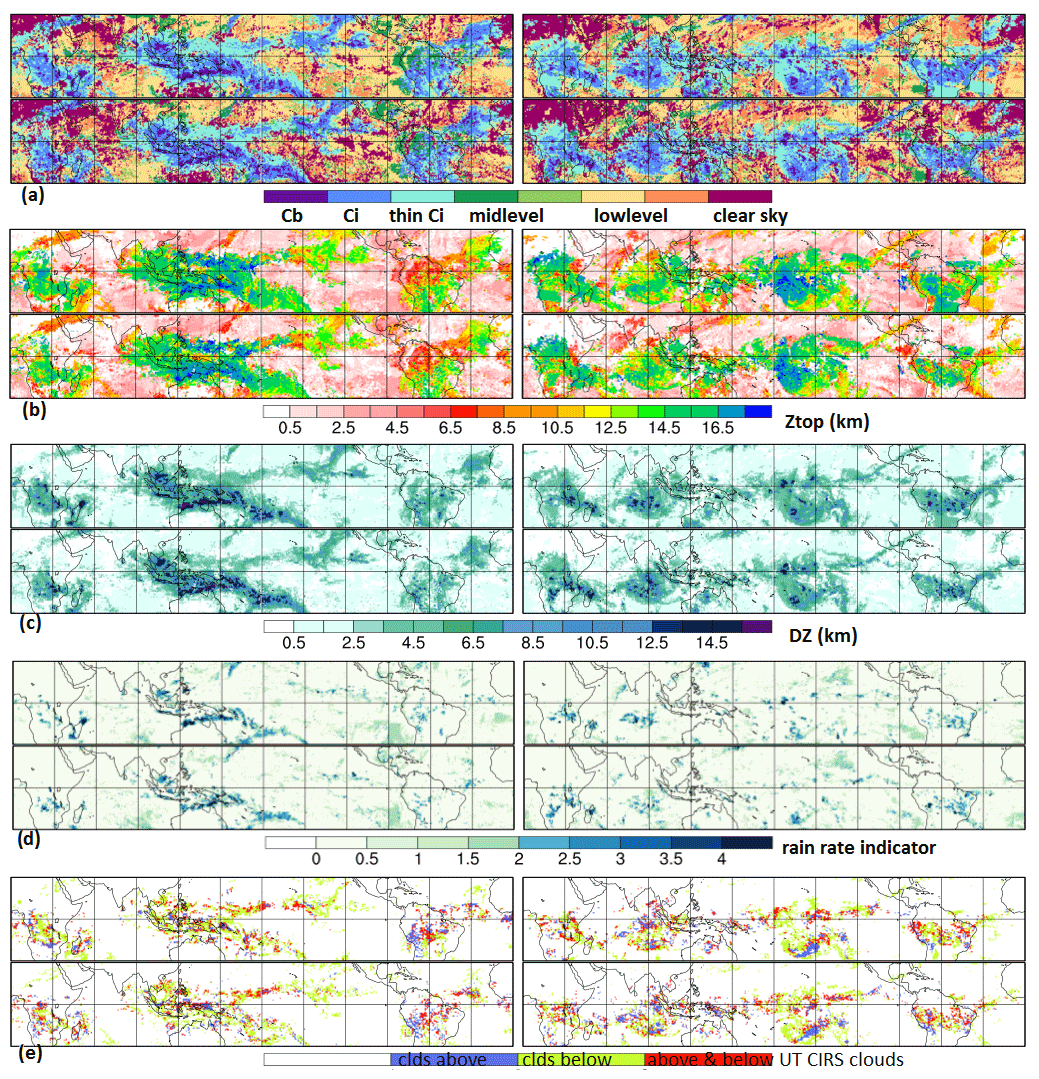
Figure 2 Horizontal structure for one specific day during a La Niña (left) and El Niño situation (right) at 01:30 and at 21:30 LT of (a) CIRS scene type (b) cloud top height, (c) cloud vertical extent, (d) rain rate indicator and (e) cloud layers in addition to the identified UT clouds by CIRS.

When investigating monthly mean anomalies in the time series, we have seen a small artificial peak for the rain rate indicator in March 2014 for the AIRS observations. This peak was larger for the first model than for the second model. Therefore we show in the following all results using the second model which does not include predicted variables as input for the rain rate classification. At the end of this disturbance, most probably evoked by cosmic particles during a solar flare event, the AIRS instrument shut down on 22 March, as its electronic circuit was affected. The instrument was operational again by the end of March. No obvious failure is seen in the retrieved cloud variables, but many small areas with strong rain rate appear during this period.

2.4 UT cloud system reconstruction

The cloud system reconstruction (Protopapadaki et al., 2017) is based on two independent variables, p_cld and ε_cld, over grid cells of 0.5^∘ latitude × 0.5^∘ longitude. This method is different with respect to other mesoscale cloud system analyses based on IR brightness temperature alone (e.g. Machado et al., 1998; Roca et al., 2014). After the filling of data gaps between adjacent orbits, UT cloud systems were built from adjacent elements, containing at least 90 % UT clouds (p_cld < 440 hPa) of similar cloud height (within 6 hPa × ln(p_cld[hPa]), which corresponds to 27 hPa for p_cld=100 and to 37 hPa for p_cld=400 hPa). In a next step, the cloud emissivity was used to distinguish between convective cores (ε_cld > 0.98), cirrus anvil (0.98 > ε_cld > 0.5) and surrounding thin cirrus (0.5 > ε_cld > 0.05). In order to reduce the noise in the determination of the number of convective cores, one searches for grid cells with ε_cld > 0.98 within regions of ε_cld > 0.93. The convective core fraction within a MCS is then the total number of these grid cells divided by the number of grid cells belonging to the whole system, and the number of convective cells corresponds to the number of regions with ε_cld > 0.93 which include at least one grid cell with ε_cld > 0.98. Each of these regions with at least one such grid cell counts as a convective core. With this definition, the mesoscale UT cloud system coverage is about 20 % within the latitude band 30^∘ N–30^∘ S. MCSs with at least one convective core cover 15 % of this latitude band, while the coverage of all UT clouds (p_cld < 440 hPa) is about 35 %.

Figure 3 compares the normalized frequency distributions of the normalized vertical extent of the convective cores, cirrus anvils and surrounding thin cirrus within the MCSs for the 30 % warmest (SST > 302 K) and coolest (SST < 300 K) tropical ocean. As expected, this variable is close to 1 for a convective tower, with a peak of the distribution at 0.8 for convective cores, and decreases with the optical depth or emissivity of the anvil parts, with a peak of the distribution at 0.2 for the surrounding thin cirrus. While the distributions of convective cores and thin cirrus are well separated, the distribution of the cirrus anvils lies in between. The overlapping between cirrus anvils and convective cores is however larger over the cooler ocean regions. This indicates that the convective cores in these regions are probably less well defined by ε_cld > 0.98 than the ones of the MCSs in the warmer regions, the latter being more convective (e.g. Fig. 10 of Stubenrauch et al., 2021). Since we now have the normalized vertical cloud extent from the machine learning, we use it to improve the definition of convective cores, by adding the condition DZ $/z_{\mathit{top}}$ > 0.6 (cloud filling more than 60 % between the surface and cloud top). All grid cells which do not fulfill the condition DZ $/z_{\mathit{top}}$ > 0.6 are then counted back as cirrus anvil.

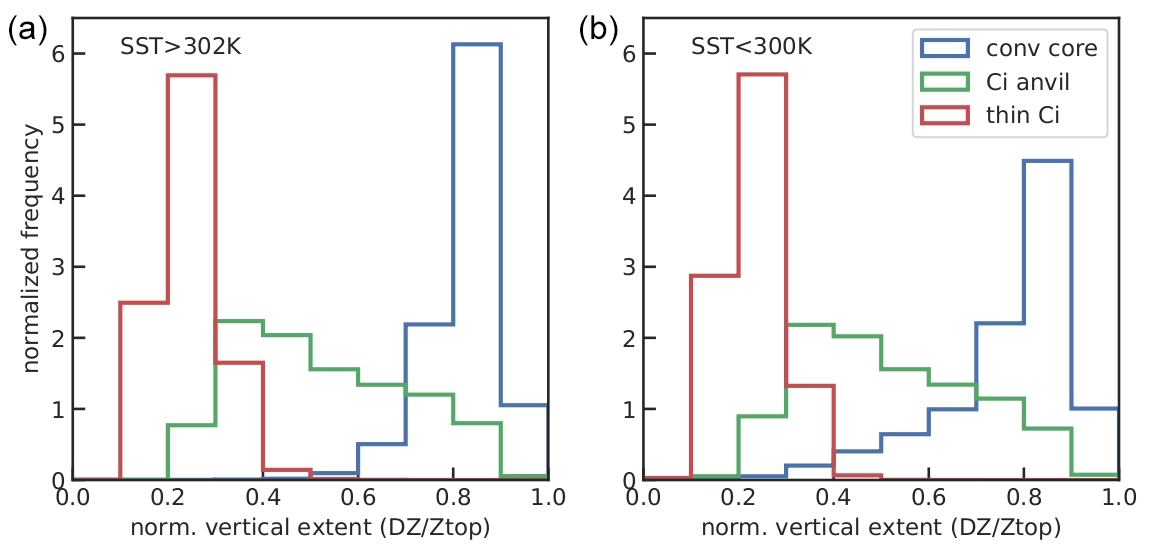
Figure 3 Density distributions of normalized vertical extent (DZ $/Z_{\mathrm{top}}$) of MCS convective cores, Ci anvils and surrounding thin Ci, separately over the 30 % warmest regions (a) and over the 30 % coolest regions (b) over ocean. Statistics are for 2008–2018.

2.5 Indicators of tropical convective organization

Convective aggregation, which refers to the clustering of convective cells, occurs at multiple spatial scales in the tropics. Organized convection, leading to MCSs and therefore associated to extreme precipitation, is a research subject of high interest, in particular in regard to climate warming. With the spatial resolution of our data, we are mainly able to consider the organization of MSCs into large squall lines, hurricanes or super clusters. This type of organization should be more influenced by the large-scale environment and circulation.

There are two main factors that play a role in estimating the degree of organization: the variable used to define convection (Sect. 2.5.1) and the metric used to compute the degree of organization (Sect. 2.5.2).

2.5.1 Definition of convective areas within UT clouds

Studies have used cold IR brightness temperatures (e.g. Tobin et al., 2012; Bony et al., 2020) as well as precipitation rate (e.g. Popp and Bony, 2020; Bläckberg and Singh, 2022) to define convective objects for the determination of convective organization metrics.

In order to estimate the organization of convection, measures of convection without missing data are needed. Since both AIRS and IASI data still show gaps of missing data between the orbits, we have filled these gaps with the measurements that are nearest in time. First we excluded snapshots which have a data coverage in the latitudinal band 30^∘ N–30^∘ S less than 68 % for AIRS and less than 74 % for IASI (as the swath is slightly larger for IASI). This ensures complete orbits. As described in Sect. 2.3, gaps between orbits are then iteratively filled by using the observations closest in time. In general with four observations per day, we get complete snapshots (coverage larger than 99.5 %).

In general, strong vertical updraft, strong precipitation and very cold and optically thick cloud tops indicate deep convective towers (e.g. Machado et al., 1998; Liu and Zipser, 2007; Yuan and Houze, 2010). Cold and optically thick cloud tops can be identified by a threshold in IR brightness temperature, T_B, a measurement available by any radiometer aboard geostationary and polar orbiting satellites over a long time period. However, as this variable depends on both cloud height and emissivity (Fig. 2 of Protopapadaki et al., 2017), for T_B > 230 K, very cold semi-transparent cirrus may be misidentified as lower opaque clouds, leading to uncertainties in the sizes of the convective areas.

Figure 4 compares latent heating (LH) profiles derived from the precipitation radar measurements of the Tropical Rain Measurement Mission (TRMM) for the same percentile statistics, using cold T_B, precipitation intensity (given by the ML-deduced rain rate indicator) and horizontal extent of rain within each grid cell of 0.5^∘ (given by the fraction of any precipitation deduced by ML). These LH profiles have been retrieved by the Spectral Latent Heating (SLH) algorithm (Shige et al., 2009) and are averaged over 0.5^∘. The time interval with the AIRS–CIRS data are within 20 min. The same percentile statistics allows to directly compare the efficiency of each variable to identify large latent heating, an indicator of deep convection. In all cases, the LH increases with decreasing T_B, increasing rain rate indicator and increasing horizontal rain coverage per grid cell, showing that both variables can be used as proxies for deep convection. Moreover, at fixed percentiles, the ML-derived rain rate indicator as well as the grid cell rain coverage both lead to a larger LH than T_B. This means that the ML-derived rain rate classification, together with the CIRS identification of UT clouds, is a slightly better proxy for regions of large latent heating than T_B.

Figure 4 Comparison of latent heating rate profiles from TRMM (Shige et al., 2009) averaged over the same percentile statistics, using the coldest brightness temperature (T_B), the largest rain rate indicator (b) and the largest spatial extension of rain within a grid cell of 0.5^∘ (a). Since the grid cell precipitation coverage saturates at 1, one can only go down to the 10 % largest cover. Statistics of collocated TRMM – AIRS data in the period 2008–2013.

2.5.2 Convective organization indices

It is not easy to define suitable organization metrics. The organization index I_org (e.g. Tompkins and Semie, 2017) compares a cumulative distribution of nearest-neighbour distance (NNCDF) to the one expected by randomly distributed points in the domain. I_org lies between 0 and 1, with 0.5 corresponding to randomly distributed objects. I_org > 0.5 indicates an organized state. However, Weger et al. (1992), who initially developed this method to study the distribution of cumulus clouds, pointed out that the NNCDF is sensitive to the number of areas and to their size, in particular when the total area is larger than 5 % to 15 % of the studied domain: in that case, possible merging of the objects leads to an artificial decrease of I_org. When using I_org, one has therefore to use a proxy for the definition of convective areas which corresponds to a total area that only covers a small fraction of the region to be studied.

Therefore White et al. (2018) developed the convective organization potential (COP), by assuming that 2D objects that are larger and closer together are more likely to interact with each other in the horizontal plane. It uses the distance between the centres of the objects and radii of equal area circles. Jin et al. (2022) have further developed COP to the area-based convective organization potential (ABCOP) by using the area rather than the radius and by changing the distances between centres to distances between outer boundaries. Furthermore, the interaction potentials are computed for only one pair per aggregate and summed up instead of averaged over all pairs. ABCOP is however very sensitive to the total area of the objects (Sect. 3.3).

The Radar Organization MEtric (ROME) developed by Retsch et al. (2020) considers the average size, proximity and size distribution of the convective objects in a domain and is similar to COP, but like ABCOP, it employs the distance between the outer boundaries. ROME defines interactions between pairs by assigning a weight to each pair that decreases with the distance and increases essentially with the area of the larger object, adding a contribution of the smaller area, depending on the separation distance. It is given in units of km² and lies between the mean area of the objects and twice their mean area. Hence ROME is very sensitive to the mean areas of the objects (Sect. 3.3).

3 Results

As application examples, we highlight results from analyses using this long-term 3D dataset. We particularly concentrate our interest on the ML-derived rain rate indicator. Section 3.1 shows the coherence of this newly derived variable. The cloud system approach enables us to study the behaviour of the MCSs with respect to their life cycle stage and convective depth. This process-oriented analysis presented in Sect. 3.2 can be used to evaluate parameterizations in climate models (Stubenrauch et al., 2019). In Sect. 3.3, we show results concerning mesoscale convective organization. Mesoscale convective organization has been identified by larger and higher systems, which also live longer than unorganized systems (e.g. Rossow and Pearl, 2007; Takahashi et al., 2021), and they also lead to increases in tropical rainfall (e.g. Tan et al., 2015). We first compare convective organization indices derived from objects defined by strong rain and by cold cloud temperature and then investigate changes in geographical patterns of radiative heating with respect to one of these indices (I_org).

3.1 Coherence of ML-derived rain intensity classification

First we test the coherence between the ML-derived rain rate classification and the collocated TRMM LH profiles already presented in Sect. 2.5.1. Figure 5 compares the LH profiles averaged over all UT clouds and over all mid- and low-level clouds and separately over those with no rain, light rain and heavy rain according to the rain rate classification described in Sect. 2.3. Indeed, when the rain rate classification indicates no rain, the latent heating from TRMM is very small. The latent heating is on average about 10 (5) times larger for grid cells which include heavy precipitation than the tropical average for UT clouds (mid- and low-level clouds). While latent heating profiles have a peak between 400 and 500 hPa for heavily precipitating UT clouds, the peak lies around 850 hPa for strongly precipitating mid- and low-level clouds. This indicates that the ML-derived rain rate classification seems to be coherent for UT clouds as well as for lower clouds, though the noise for the latter may be larger.

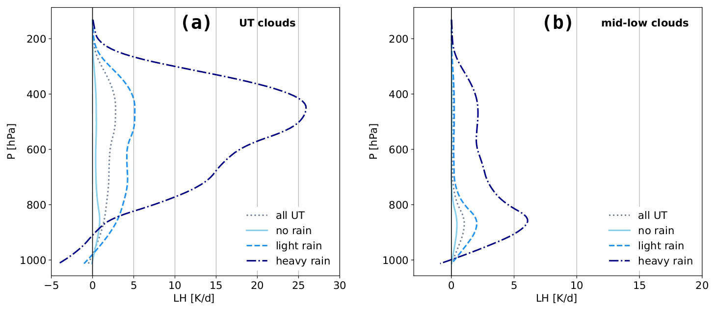
Figure 5 Latent heating profiles derived from TRMM averaged over UT clouds (a) and over mid- and low-level clouds (b) identified by AIRS. In addition means over non-precipitating, lightly precipitating and heavily precipitating clouds are shown. These precipitation conditions are given by the rain rate indicator classification derived from ML models applied to AIRS–ERA-Interim and trained with CloudSat. Statistics of collocated TRMM–AIRS in the period 2008–2013.

Figure 6 compares normalized frequency distributions of ε_cld, z_top, cloud fuzziness and normalized vertical extent of non-precipitating, lightly and heavily precipitating UT clouds. From these figures, we clearly deduce that heavily precipitating UT clouds in the tropics have an emissivity close to 1, are in general higher, have a much less fuzzy cloud top and a much larger vertical extent than non-precipitating UT clouds. These results are coherent with expectations and again confirm the quality of the rain rate classification derived by our machine learning procedure.

Figure 6 Density distributions of (a) cloud emissivity, (b) cloud top height, (c) cloud fuzziness and (d) normalized cloud vertical extent, for non-precipitating, lightly precipitating and heavily precipitating UT clouds. Statistics are for 2008–2015 at 01:30.

3.2 Process-oriented behaviour of mesoscale convective systems

The cloud system concept described in Sect. 2.4 permits us to link the convective core and anvil properties: the fraction of the convective core area within a cloud system indicates the life cycle stage (e.g. Machado et al., 1998), with a large fraction indicating the developing stage and a decreasing fraction during dissipation. Once the systems have reached maturity, the minimum temperature within a convective core is a proxy for the convective depth.

According to Takahashi et al. (2021), using a convection-tracking analysis on data from Intergrated Multisatellite Retrievals for GPM (IMERG), the fraction of precipitating cores (adjacent grid cells with a rain rate > 5 mm h⁻¹) within precipitation systems (adjacent grid cells with rain rate > 0.5 mm h⁻¹) first increases and then decreases during the evolution of these systems. The maximum of the strong rain area relative to the whole precipitating area as well as the maximum and average intensity of the precipitation increase with the lifetime of the systems. This behaviour was also found by Roca et al. (2017).

Our data do not provide the absolute system lifetime, but the convective core fraction within a system indicates the maturity stage in a normalized life cycle. Figure 7 presents the statistical evolution during the life cycle of (a) the precipitating area relative to the whole MCS area and (b) the strong rain area relative to the precipitating area, for single core MCSs. As the rain rate classification was obtained per CIRS footprint, a grid cell of 0.5^∘ × 0.5^∘ can be declared as precipitating by using different thresholds on the fraction of footprints with rain rate > 0 mm h⁻¹. The same applies for grid cells including strong rain. Results using three different thresholds to define the precipitating and strongly precipitating areas are compared. For all thresholds, the precipitating area is very large in the beginning of the life cycle, when the anvil is just developing and then decreases, while the fraction of strong rain stays constant until the anvil reaches 40 % of the system size and only then decreases. With our coarse spatial resolution we did not see the increase in strong rain after the developing stage, which has been observed by Fiolleau and Roca (2013) and Takahashi et al. (2021), using data with better time and space resolution. This means that we miss the very first development of the convective tower itself, as can also be seen in Fig. 7c, which presents the evolution of the convective core size and the convective core top height. The latter varies much less than the convective core size, with an average of already 12.8 km for a convective core fraction close to 1. So due to the coarse spatial resolution and considering only high-level clouds, we start to identify the systems when they are already near to their maximum height, which is attained just before the decrease of the heavy rain portion.

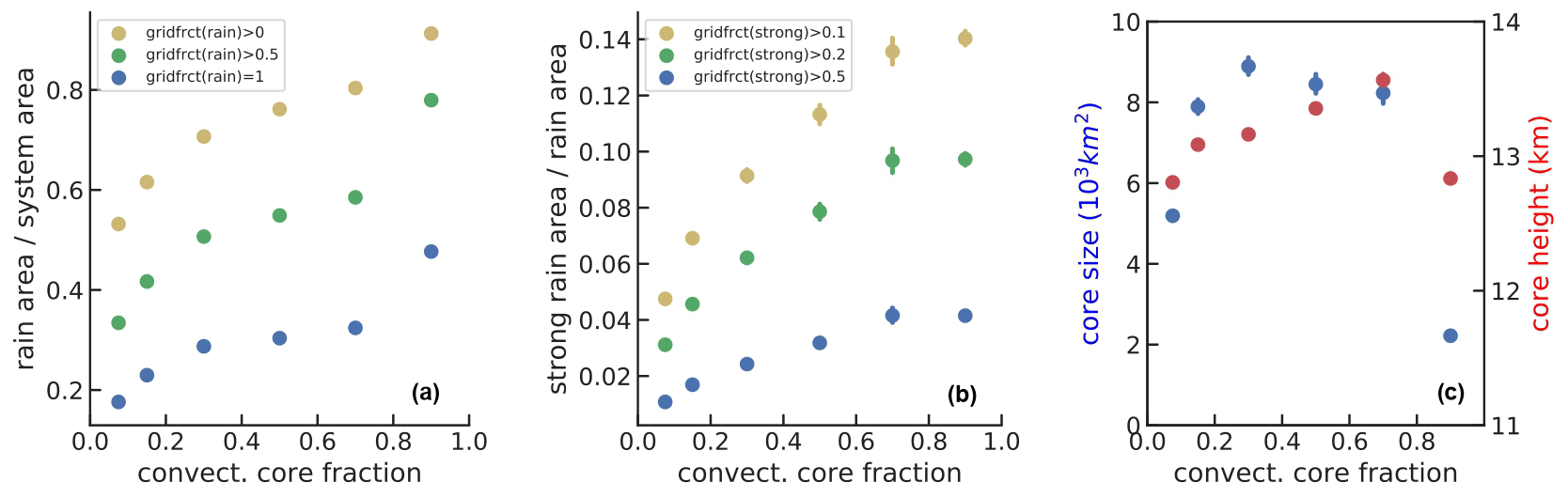
Figure 7 MCS properties as a function of their life cycle stage, given by fraction of convective core area within the system (1 corresponds to developing phase with no anvil and 0.1 to dissipating stage). Only cloud systems with a single convective core are considered: (a) ratio of precipitating area over MCS size, (b) ratio of strong rain area over precipitating area and (c) size and top height of the convective cores. For (a) and (b), different thresholds on the rain fraction per grid cell are compared. The condition on strong rain also includes the condition that at least 50 % of the grid cells are covered by any rain. Statistics combine observations at 01:30 and 13:30, for 2008–2018.

The core size increases rapidly and then stays stable until dissipation of the system. We identify MCS maturity by a core fraction between 0.2 and 0.4, because by then the core size has attained its maximum.

Once the convective systems are mature, we can study their properties with respect to their convective depth: Fig. 8 presents, as a function of the minimum temperature within the convective cores, (a) the strong rain area relative to the precipitating area (again considering three thresholds); (b) the volume of the thick anvil (ε_cld > 0.5) relative to the volume of the convective core, which is a proxy for detrainment, and the emissivity of the thick anvil; and (c) the size of the surrounding thin cirrus relative to the total anvil size as well as the 50 % warmest surface temperature underneath the MCSs. We deduce that deeper convection clearly leads to (1) larger areas of heavy rain within the precipitating areas, in agreement with earlier studies; (2) a larger volume detrainment but with a slightly smaller emissivity; and (3) more surrounding thin cirrus. From Fig. 8 we also conclude that deeper convection occurs in general in the warmer regions of the tropics, as expected.

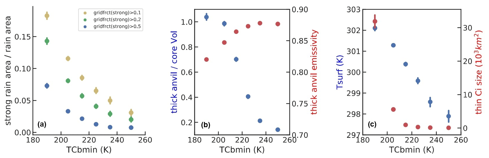
Figure 8 Mature MCS system properties as a function of their convective depth, given by decreasing minimum temperature within the convective cores: (a) ratio of strong rain area over precipitating area, (b) volume detrainment and thick anvil emissivity and (c) 50 % warmest surface temperature underneath the MCSs and ratio of thin cirrus over total anvil area. For (a), different thresholds on the fraction of strong rain per grid cell are compared, and at least 50 % of the grid cells are covered by any rain. Statistics combine observations at 01:30 and 13:30, for 2008–2018.

3.3 Tropical convective organization

In this section we demonstrate the usefulness of this new dataset by analyzing the convective organization in the tropics. We compare results using various metrics of convective organization and proxies to define convective objects, as described in Sect. 2.5. A spatial resolution of 0.5^∘ relates to an organization of MSCs at a scale which is more linked to the large-scale environment and circulation. We first consider the annual cycle of convective organization and then highlight an application on interannual variability.

Figure 9 presents the annual cycle of (a) I_org, (b) ROME, (c) COP, (d) total area and (e) mean area of the convective objects and (f) their number. We also investigate different variables to define these objects, in particular precipitation intensity (given by ML-derived rain rate indicator) of UT clouds (p_cld < 350 hPa) and cold cloud temperature (T_cld < 230 K) of opaque clouds (ε_cld > 0.95). The latter definition is similar to T_B < 230 K but without any contamination of colder, thinner Ci. Since ROME is strongly related to the size of the convective objects, we have also computed the annual anomalies of the three indices by using only 2 % of the largest precipitation intensities for constructing the convective objects. This corresponds to comparing the indices for a constant total area of convection. A similar approach was undertaken in a study by Bläckberg and Singh (2022), using the precipitation intensity and ROME as proxies for convection and convective organization, respectively.

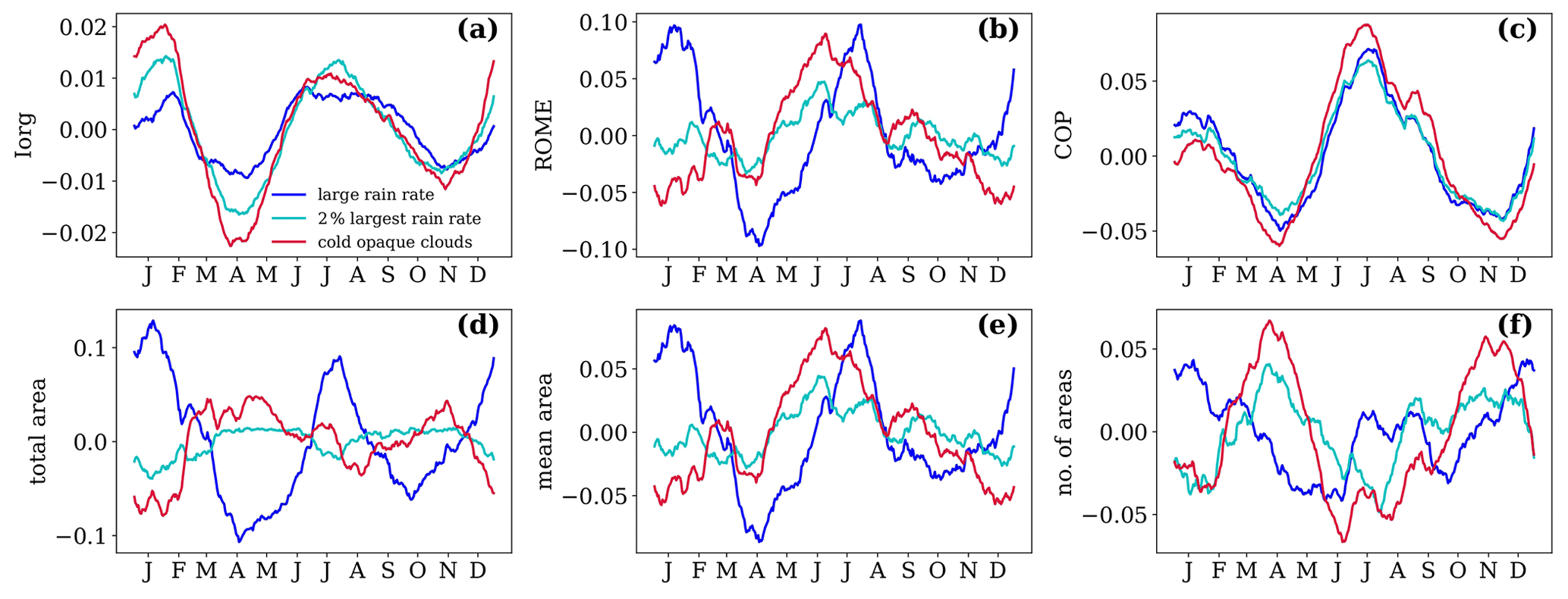
Figure 9 Annual cycle of (a) I_org, (b) ROME, (c) COP, (d) total area of convective objects, (e) mean convective area and (f) number of convective areas. These areas are built from grid cells covered by at least 90 % UT clouds, with rain rate indicator > 2 (dark blue), T_cld < 230 K and ε_cld > 0.95 (red), or using the 2 % largest rain rate indicator values (cyan). The latter leads to a constant total area of convection. Monthly statistics of UT clouds averaged over four observation times from 2008–2018.

All three indices reveal a clear annual cycle of convective organization, with a minimum in April and November and a maximum in July and August and in January and February, though with differences in magnitude and width of the oscillations due to the choice of proxy for convective area. While the amplitude of the annual cycle is the smallest for I_org (0.04), the seasonal anomalies of COP are the less sensitive and those of ROME the most sensitive to the choice of proxy. The latter look very similar to those of the mean area of the convective objects (with a correlation coefficient larger than 0.9). Thus the seasonal anomalies of ROME primarily reflect the ones of the mean areas of the convective objects. We also observe in Fig. 9e that the minima and maxima in the annual cycle of the mean area of objects with intensive rain are shifted compared to those with cold opaque cloud. When using a fixed total area of intense precipitation, the magnitude of the seasonal anomalies is much smaller and the shift in behaviour compared to using the proxy of cold opaque clouds disappears.

The annual cycle of the total area of convective objects can be reconstructed by the one of the mean area times the one of the number of the convective objects (Fig. 9d–f): the relative flatness of the seasonal cycle of the total area of cold cloud objects can be explained by a nearly opposite seasonal cycle in their mean size and number, whereas for intense precipitation their cycles are in phase which then leads to a pronounced cycle in their total area.

The absolute values of the convective organization indices, presented in Fig. S3 of the Supplement, depend more strongly on the proxy used to define the convective objects: the absolute maximum of COP is the same for all proxies during boreal summer, while for other seasons, COP, like I_org, is larger when considering precipitation intensity. While ROME primarily reflects the mean area, ABCOP reflects the total area of the convective objects (both with a correlation coefficient larger than 0.8). Whereas the mean area of the convective objects is clearly an indication of mesoscale convective organization, the total area may not be directly linked to convective organization, only perhaps if one considers local regions. I_org, only considering the distance between convective objects, seems to add another aspect. I_org indicates a more organized convection when precipitation intensity is used instead of cold cloud temperature to identify the convective objects, though the total area of intense precipitation areas is smaller than the one of the cold cloud objects. The difference in the absolute peak values of the I_org and COP anomalies between boreal summer and boreal winter may be explained by regional shifts in intense precipitation occurrence, as shown in Fig. S4 and in agreement with earlier results (e.g. Berry and Reeder, 2014).

Figure 10 presents the annual cycle of MCS properties discussed in the earlier sections: the core height of the MCSs, the anvil horizontal detrainment estimated by the ratio of anvil over convective core size and the vertical extent of the anvil (Fig. S5) are in phase with the annual cycle of I_org and COP. This shows that in seasons with larger tropical convective organization, the MCSs have in general higher cloud tops and larger anvils. The fraction of single-core MCSs and the ratio of thin cirrus over total anvil size are in opposite phase. The first confirms that convective organization corresponds to multi-core MCSs. The latter may not be directly expected as we have seen that this ratio increases with the height of the MCSs (convective depth). On second thought, it may be explained by the fact that clustering of convective systems leaves less space for the thin cirrus between them. It is interesting to note that the annual cycle of the relative subsidence area (clear sky and low-level clouds) is also in phase with the one of I_org and COP. This means that larger heating of the upper and middle tropospheric heating by more organized MCSs leads to more cooling of the lower troposphere in the subsidence regions, which has recently been found by Stubenrauch et al. (2021).

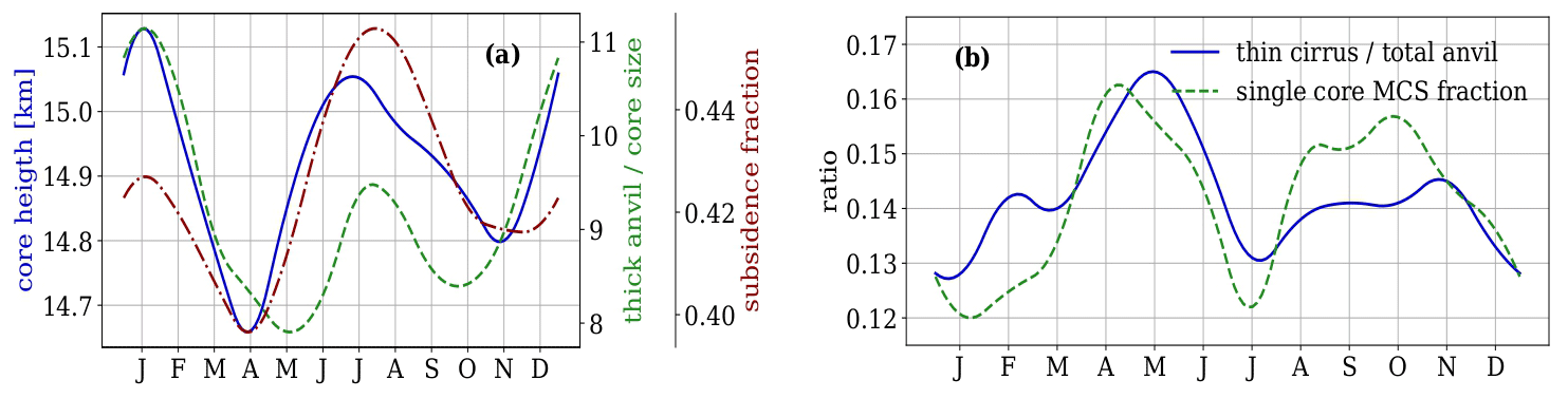
Figure 10 Right: annual cycle of (a) MCS core top height (blue), horizontal detrainment (green) and fraction of subsidence area (given by clear sky and low-level clouds) over the tropics (red), and (b) ratio of thin cirrus over total anvil size (blue) and fraction of single core MCSs (green). Monthly statistics averaged over four observation times from 2008–2018.

Changes in gradients of tropospheric radiative heating relate to changes in atmospheric circulation. We link interannual anomalies of the 3D radiative heating rate (HR) fields of Stubenrauch et al. (2021) to those of I_org over the period from 2008 to 2018. In order to remove the seasonal dependency, we computed the 121 12-month running mean anomalies for these variables. The geographical distribution of changes in radiative heating with respect to convective organization are presented in Fig. 11, separately for the upper, middle and low troposphere and for the two proxies to define convective objects. These geographical maps have been obtained by linear regression per grid cell of the 121 pairs of heating rate and I_org anomaly (see examples in Fig. S6 in the Supplement).

The geographical patterns and magnitudes in HR change with respect to change in I_org are similar for both proxies but with slightly larger derivatives for strong precipitation areas. This may be expected as intense precipitation should be a more direct proxy for convection than cold cloud top. In general the derivatives are large because interannual changes in I_org are very small, as shown in Fig. 12. In the upper troposphere, we observe increased heating north and south of the Equator in the Central Pacific and a decrease over the Warm Pool, while in the middle and low troposphere there is an increase in heating around the Equator over the whole Pacific and Indian Ocean and a decrease in heating over the Warm Pool and in the Atlantic. The HR pattern changes in the convective regions are induced by relative changes of thin cirrus, cirrus and high opaque clouds, which are similar but not identical to the ones related to the El Niño–Southern Oscillation (ENSO) during this period (Fig. S7), with increasing convection close to the Equator and increasing cirrus and thin cirrus around the Equator. Indeed, the correlation between I_org and the oceanic Niño index (ONI) is positive (with correlation coefficients of 0.7 and 0.3 for cold cloud temperature and precipitation intensity as a proxy, respectively). In the stratocumulus regions off the western coasts of the Americas and of Australia there seems to be less cooling in the low troposphere, probably due to a recent reduction in low-level clouds, in particular in the NE Pacific, which was found in coincidence with a shift in the phase of the Pacific Decadal Oscillation (Loeb et al., 2018, 2020; Sun et al., 2022). The similarity between the maps obtained with the two selections validates once again the reliability of the rain rate indicator obtained with ML. The slightly stronger patterns lead to the conclusion that strong precipitation is a slightly better proxy to define convective areas than cold temperature.

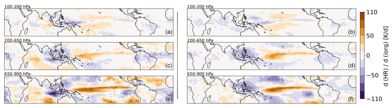
Figure 11 Change in radiative heating rates with respect to deseasonalized I_org computed from convective areas defined by grid cells with rain indicator > 2 and by grid cells with T_cld < 230 K and ε_cld > 0.95 . The troposphere is divided into three layers: (a, b) upper troposphere (100–200 hPa), (c, d) mid-troposphere (200–600 hPa) and (e, f) low troposphere (600–900 hPa). Monthly statistics from 2008–2018.

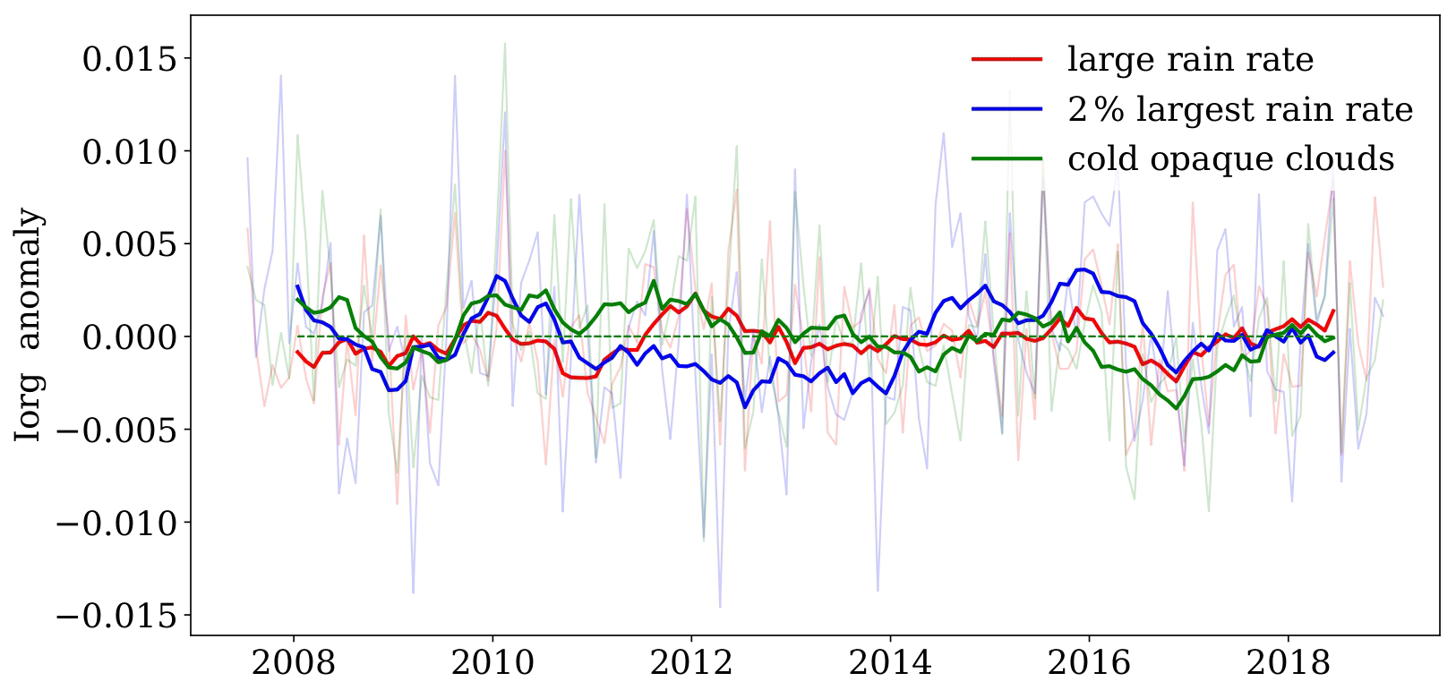
Figure 12 Time series of deseasonalized monthly anomalies of I_org, using different proxies to define the convective areas. The deseasonalization was done by computing 12-month running means. The monthly anomalies are shown in light grey.

Whereas the geographical patterns of the derivatives of heating/cooling with respect to I_org show a coherent picture, we did not find any correlation between the very small interannual anomalies of I_org (shown in Fig. 12) and the ones of the tropical means of different variables like surface temperature, thin cirrus area and subsidence area. The correlations depend on the proxies for the definition of the convective areas and in particular on the metrics for convective organization. Already the time series of the interannual anomalies of the different indices have a different behaviour as can be seen in Fig. S8 in the Supplement. We have also investigated tighter thresholds on the variables which define deep convection (like rain rate indicator > 2.5 or T_cld < 210 K); however we are left with only about 0.5 % total area, which increases the noise level. In addition, we found that the results also change when we exclude objects with the size of only one grid cell (not shown), as already pointed out by Jin et al. (2022). Therefore we do not consider it meaningful to use the discussed convective organization indices for an estimation of tropical mean changes with respect to changes in convective organization.

While we have seen that the convective organization indices vary much more seasonally than interannually, Fig. 13 suggests that the difference of the density distributions of convective core height and strong rain area within the MCSs between April and July or between cool years (2008/2011) and warm years (2015/2016) is of the same order, with a shift towards higher core height and a longer tail in strong rain area. However, the size distributions of the MCSs are similar. The tail in the mean area of strong precipitation within the MCSs is clearly larger in the case of warmer years. This indicates that a shift in tropical surface temperature changes only a small part of the MCSs, with more extreme values. Such behaviour cannot be identified using a convective organization index computed over the whole tropics.

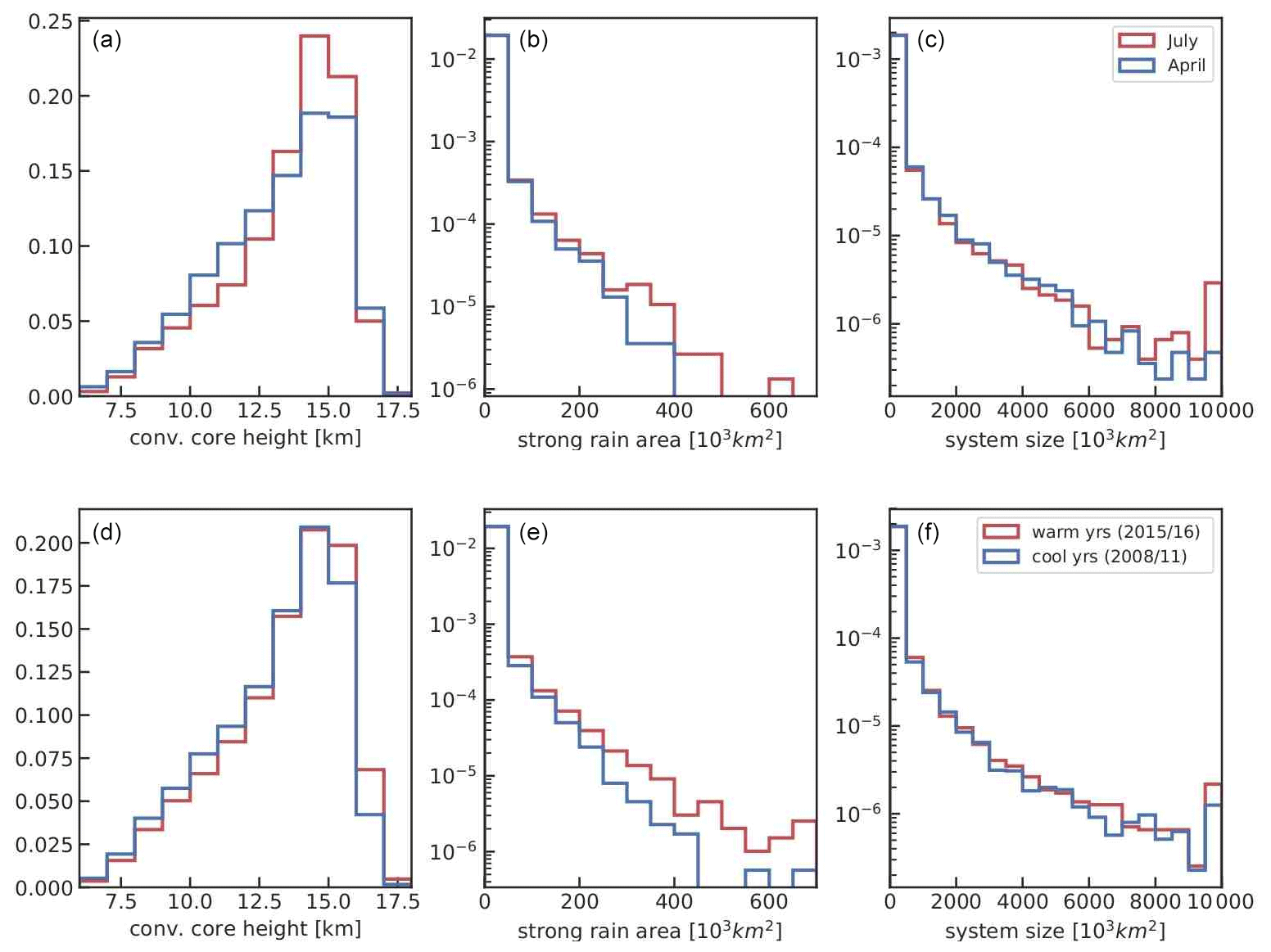
Figure 13 Density distributions of MCS system properties, comparing April and July (a, b, c) and cooler and warmer years (d, e, f): height of convective cores (a, d), size of areas with strong precipitation (b, e) and system size (c, f). Statistics combine observations at 01:30 and 13:30, for 2008–2018, for MCSs with core fraction > 0.1.

4 Conclusions and outlook

We have presented a methodology to extend spatially and temporally information on the cloud vertical structure and precipitation derived from active lidar and radar measurements of CALIPSO and CloudSat missions. This new approach made use of CIRS data obtained from advanced IR sounder measurements of AIRS and IASI combined with ERA-Interim reanalyses and machine learning technologies using ANN. The resulting 3D dataset of UT cloud systems, covering 2008–2018, together with a similarly produced dataset of radiative heating rates (Stubenrauch et al., 2021), can be used to improve our understanding of the relationship between tropical convection and resulting anvils and how they are impacted by and feed back to climate change.

Though the uncertainties in the predicted variables and classifications are relatively large (with an accuracy of about 65 % to 70 % for the rain intensity classification), this new dataset allows to study their horizontal structures on specific snapshots in time. For a complete instantaneous coverage, necessary to compute indices of tropical convective organization, the gaps between the orbits have been filled iteratively with the four observations per day of AIRS and IASI data, starting with those closest in time (already leading to 90 % coverage). We have demonstrated that the newly developed precipitation intensity classification is slightly more efficient to detect large latent heating and therefore deep convection compared to the cold cloud temperature.

The cloud system approach developed by Protopapadaki et al. (2017) has been slightly modified, and the normalized vertical extent obtained from the ML approach has been employed to slightly improve the identification of the convective cores, in particular in the cooler tropical regions. The cloud system concept allows a process-oriented evaluation of parameterizations in climate models. In agreement with earlier studies (e.g. Schumacher and Houze, 2003; Roca et al., 2014; Takahashi et al., 2021), we found that deeper convection leads to larger areas of heavy rain. These results also confirm the quality of the ML-derived precipitation rate classification. With increasing convective depth, mature MCSs also show an increase in volume detrainment, while the anvil emissivity slightly decreases.

Moreover we have shown the usefulness of our new dataset by investigating convective organization metrics. By comparing different organization indices (I_org, COP, ABCOP and ROME) and proxies to define convective objects, we have shown that the indices indicate a similar annual cycle of convective organization. However, ABCOP and ROME are strongly correlated to the total and mean area of the objects, respectively. While the mean area of the objects is certainly an indication of convective organization, their total area at tropical scale seems to be less linked to organization. The index I_org, which only considers the distance between convective objects, seems to add another information. The core height of the MCSs and their anvil detrainment are in phase with the annual cycle of I_org and COP, as well as the relative subsidence area. This also shows a link between the MCSs and subsidence areas. It is interesting to note that the annual cycles of the total area of cold cloud objects and of intense precipitation objects are very different. This can be related to a nearly opposite cycle in their mean size and number for the first and to a cycle in phase for the latter.

Changes in gradients of tropospheric radiative heating relate to changes in atmospheric circulation. The geographical patterns and magnitudes in radiative heating rate changes with respect to I_org are similar for both proxies but slightly larger for strong precipitation areas. This may be expected as intense precipitation should be a more direct proxy for convection than cold cloud top. Furthermore, the HR pattern changes are similar to the ones related to ENSO during this period.

However, the time series of the interannual anomalies of convective organization strongly depend on the convective organization metrics, and correlations between these anomalies and those of tropical means of different atmospheric variables do not show consistent results. The tail of the distribution of strong rain areas seems to be more related to warmer tropics than the indices themselves. Therefore one has to be careful using only one of these organization indices and proxies to study climate change. More detailed studies are necessary to show the behaviour of these indices with spatial resolution and domain size.

This database of UT cloud systems, their vertical structure and precipitation areas is being constructed within the framework of the GEWEX (Global Energy and Water Exchanges) Process Evaluation Study on Upper Tropospheric Clouds and Convection (GEWEX UTCC PROES) to advance our knowledge on the climate feedbacks of UT clouds. It will be made available within this year via https://gewex-utcc-proes.aeris-data.fr/. For the future it will also be interesting to use this dataset for the study of cold pools, using data of Garg et al. (2020).

In order to continue this dataset beyond 2018, we are now preparing a new version of CIRS data, using ERA5 (Hersbach et al., 2020) instead of ERA-Interim ancillary data, and newly calibrated AIRS L1C radiances (Manning et al., 2019) as input.