the Creative Commons Attribution 4.0 License.
the Creative Commons Attribution 4.0 License.
 | 26 May 2023
Changes in global teleconnection patterns under global warming and stratospheric aerosol intervention scenarios
Abolfazl Rezaei
Khalil Karami
Simone Tilmes
John C. Moore
We investigate the potential impact of stratospheric aerosol intervention (SAI) on the spatiotemporal behavior of large-scale climate teleconnection patterns represented by the North Atlantic Oscillation (NAO), Pacific Decadal Oscillation (PDO), El Niño–Southern Oscillation (ENSO) and Atlantic Multidecadal Oscillation (AMO) indices using simulations from the Community Earth System Model versions 1 and 2 (CESM1 and CESM2). The leading empirical orthogonal function of sea surface temperature (SST) anomalies indicates that greenhouse gas (GHG) forcing is accompanied by increases in variance across both the North Atlantic (i.e., AMO) and North Pacific (i.e., PDO) and a decrease over the tropical Pacific (i.e., ENSO); however, SAI effectively reverses these global-warming-imposed changes. The projected spatial patterns of SST anomaly related to ENSO show no significant change under either global warming or SAI. In contrast, the spatial anomaly pattern changes pertaining to the AMO (i.e., in the North Atlantic) and PDO (i.e., in the North Pacific) under global warming are effectively suppressed by SAI. For the AMO, the low contrast between the cold-tongue pattern and its surroundings in the North Atlantic, predicted under global warming, is restored under SAI scenarios to similar patterns as in the historical period. The frequencies of El Niño and La Niña episodes modestly increase with GHG emissions in CESM2, while SAI tends to compensate for them. All climate indices' dominant modes of inter-annual variability are projected to be preserved in both warming and SAI scenarios. However, the dominant decadal variability mode changes in the AMO, NAO, and PDO induced by global warming are not suppressed by SAI.
- Article
(3481 KB) - Full-text XML
-
Supplement
(1554 KB) - BibTeX
- EndNote


Although the Paris Agreement and accompanying international commitments to decrease carbon emissions are an essential step forward, current national contributions have only about a 50 % chance to restrict global mean temperature increase to 2 ∘C above preindustrial (Meinshausen et al., 2022). Exceeding 2 ∘C will lead to severe consequences and societal disruption worldwide, as humanity is critically dependent on ecosystems, food, fresh water, and health systems, which face rapidly challenging adaptation pressure above 2 ∘C of global warming (Field and Barros, 2014).
In parallel with emissions reductions, solar radiation modification (SRM) has been suggested to limit global temperature increases and consequent climate impacts from anthropogenic greenhouse gas (GHG) emissions. A naturally occurring analog of SRM is the well-known global surface cooling following large volcanic eruptions, albeit over relatively short periods. Simulations have shown that SRM decreasing total solar irradiance by about 2 % would roughly compensate for global warming from a doubling of CO2 concentrations (Dagon and Schrag, 2016).
Oceans act as major drivers of climate variability worldwide (e.g., Shukla, 1998; Cai et al., 2021), and more than 90 % of the excess energy balance of the earth arising from GHG emissions ends up heating the ocean (Cheng et al., 2017). Variations in sea surface temperatures (SSTs) and the global climate are linked through ocean–atmosphere energy exchanges that can be helpfully summarized by climate indices that characterize large-scale climate teleconnection patterns, that is, recurring and persistent large-scale anomaly patterns of pressure and circulation across large geographical regions. Some of the most referred to are the El Niño–Southern Oscillation (ENSO), Pacific Decadal Oscillation (PDO), Atlantic Multidecadal Oscillation (AMO), and North Atlantic Oscillation (NAO). The dominant inter-annual feature of climate variability on the planet is ENSO, and its state produces widespread climatic and environmental outcomes (Latif and Keenlyside, 2009). The PDO modulates marine ecosystems and global climate on decadal timescales (Mantua et al., 1997), impacts ENSO onset and frequency (Fang et al., 2014), and is useful for short- to long-term climate forecast (An and Wang, 1999). The AMO has broader hemispheric impacts beyond North American and European climates (Enfield et al., 2001), influencing the monsoons across North Africa, East Asia, and India (Zhang and Delworth, 2006). The NAO is among the dominant climate variability modes in the Northern Hemisphere (Simpkins, 2021).
Several studies have explored how climate indices, particularly ENSO, respond to global warming and increasing GHG concentrations. Statistically significant systemic changes have occurred in ENSO dynamics and the evolution of El Niño and La Niña events since the 1960s (Moron et al., 1998; Capotondi and Sardeshmukh, 2017). ENSO may favor more severe events under global warming (Fedorov and Philander, 2001), and Cai et al. (2015) found that ENSO-associated disastrous weather consequences tend to arise more frequently under unabated CO2 emissions. Cai et al. (2021) found an inter-model consensus on increases in forthcoming ENSO rainfall and temperature fluctuations under increasing GHG concentrations. The PDO, which is essentially the extra-tropical manifestation of ENSO, is simulated with a similar spatial pattern as at present under various future climates but with reduced amplitude and a shorter characteristic timescale (e.g., Zhang and Delworth, 2016). The North Atlantic is a key ocean for investigating global climate changes (Wang and Dong, 2010) and acts as a major carbon dioxide sink (Watson et al., 2009). Atmospheric CO2 concentrations vary with the phase of the AMO with the warm phase associated with lowered atmospheric CO2 (Wang and Dong, 2010). The two NAO action points in the Icelandic Low and the Azores High have been projected to significantly intensify and shift northeastward by 10 to 20∘ in latitude and 30 to 40∘ in longitude in response to global warming (Hu and Wu, 2004).
Stratospheric aerosol intervention (SAI) is a type of SRM that has been widely simulated by many global climate models (e.g., Kravitz et al., 2013), which is accompanied by changes in global circulations such as the NAO teleconnection pattern (Moore et al., 2014), and is known in various models to partially offset the decline in the Atlantic Meridional Overturning Circulation (AMOC; Xie et al., 2022). Undorf et al. (2018) simulated the North Atlantic SST cooling accompanied by the historical rise in stratospheric sulfate aerosol from North America and Europe dating back to 1850–1975. Gabriel and Robock (2015) is the only study to date that explores the effects of SAI in multiple models on the possible amplitude and frequency changes in the El Niño–Southern Oscillation (ENSO). They concluded that changes in ENSO in the SAI simulations were either not present or not large enough to be captured by their approach, given the across-model variability issue. Thus, little is known about possible changes that future global climate change scenarios with artificial cooling may have on ocean–atmosphere climate indices. Recently, a novel set of SRM models have been globally completed with state-of-the-art climate models: the Community Earth System Model versions 1 and 2 (CESM1 and CESM2). These models have improved planetary boundary layer turbulence, aerosols, radiation, and cloud microphysics, which should enable more reliable simulations for the forthcoming global climate change projections (Mills et al., 2017).
We use the Geoengineering Large Ensemble Simulation (GLENS) with 20 members from a single model, the Community Earth System Model 1 (CESM1) with stratospheric aerosol intervention (GLENS-SAI), to explore the possible changes in climate teleconnection patterns under future climate change scenarios. The models use the Representative Concentration Pathway (RCP) 8.5 high-GHG emissions forcing state (Riahi et al., 2011) as a baseline and increase stratospheric sulfur injections through the century to maintain global surface temperatures at 2020 levels. This produces an increasingly large signal-to-noise ratio through the 21st century. In addition, we use recent simulations (SSP5-8.5-SAI) with an updated model version (CESM2). For these simulations, the SSP5-8.5 GHG emissions scenarios were used as the GHG baseline on which SAI was performed. The two different model experiments show some surprising differences in the required sulfur injections and climate outcomes with and without SAI applications (Fasullo et al., 2020; Tilmes et al., 2020). Thus, even models from different generations in the same family can produce sufficiently different climates to explore a range of plausibly real climate impacts. The goal of this study is to identify robust features across the two model versions in the response of climate indices (ENSO, PDO, AMO, and NAO) to GHG-induced global warming and its compensation by SAI.
We employed empirical orthogonal functions and wavelet transforms to decompose time series and study the differences in the climate teleconnection patterns between the SSP5-8.5 and SSP5-8.5-SAI scenarios. Since teleconnection patterns are emergent features of the non-linear, chaotic climate system (Ghil et al., 2002), their underlying physical causes are complex and not necessarily the same in any model as on the real planet. Hence, we assess the potential changes in temporal and spatial characteristics of climate indices of the AMO, the NAO, ENSO, and the PDO under both extreme warming GHG scenarios and with SAI employed to mitigate those warmings while maintaining extreme GHG concentration trajectories.
2.1 Models and scenarios
We used two SAI models and scenarios: (1) CESM1 for GLENS-SAI and (2) CESM2 for SSP5-8.5-SAI. The GLENS simulations were done by the Community Earth System Model version 1 (CESM1) with the Whole Atmosphere Community Climate Model (WACCM) as the atmospheric system integrated to land, ocean, and sea ice models (Mills et al., 2017). The resolution of the atmospheric component is 0.9∘ in latitude and 1.25∘ in longitude. A 20-member reference simulation for the RCP8.5 scenario (Riahi et al., 2011) is available over the 2010–2030 period with three ensemble members (001 to 003) continuing up to the end of the 21st century. GLENS-SAI is a 20-member ensemble of stratospheric sulfur dioxide (SO2) injection simulations, spanning 2020–2099. Each ensemble member was begun in 2010 with small differences in their initial air temperatures, while their ocean, sea ice, and land temperatures were the same. Even before the start of the SAI injections in 2020, the fully coupled model produced variability between the ensemble members due to its chaotic nature. Here, we use all available members of the RCP8.5 and GLENS-SAI simulations, which extend until the end of the 21st century. For the analysis, we used monthly SST and sea-level pressure (PSL) from CESM1 with a duration of 1980–2009 for the historical period, 2010–2099 for global warming, and 2020–2099 for SAI.
We also analyzed output from the NCAR Community Earth System Model version 2–Whole Atmosphere Community Climate Model version 6 (CESM2(WACCM6)). This model version was used for performing the Coupled Model Intercomparison Project Phase 6 (CMIP6; Eyring et al., 2016) simulations. Like GLENS, this SAI experiment is according to the high-GHG emissions scenario, called SSP5-8.5 in CMIP6 (SSP5-8.5-SAI), and limits mean global temperatures to 1.5 ∘C above 1850–1900 conditions, which, without SAI, is exceeded around the year 2020 in CESM2(WACCM6) under SSP5-8.5. The experiment used sulfur injection locations at the same four latitudes as in GLENS to accomplish the same three temperature goals (Tilmes et al., 2020). We used the monthly SST and PSL data from all five members (r1 to r5) of the SSP5-8.5 scenario (covering 2015–2100) and the three available ensemble members of SSP5-8.5-SAI that cover the period of 2020–2100. For the analysis, we also applied a one-member historical simulation based on the specific CESM1(WACCM) version used for GLENS between 1980–2009 (denoted as historical period in the following). All three corresponding members (r1 to r3) from the CESM2(WACCM6) version were used for the historical period. For wavelet analysis modes in Sects. 2.3 and 3.2, we used the entire duration (1850–2014) of the available historical outputs from CESM2, but for spatial change patterns in Sect. 3.1, the data that cover the 1980–2009 historical period were used for consistency with CECM1.
The SAI scenarios using both CESM1 and CESM2 inject SO2 at four predefined points (30∘ N, 30∘ S, 15∘ N, and 15∘ S) at ∼5 km above the tropopause using a feedback controller to maintain not just the global mean temperature, but also the interhemispheric and Equator-to-pole temperature gradients. Fasullo and Richter (2023) explain the inter-model differences in the aerosol mass latitudinal distributions between the SAI experiments using CESM1 and CESM2. CESM2 SAI utilizes the CMIP6 SSP5-8.5 experiment as a baseline, which has been used by various modeling teams (Tilmes et al., 2020), while CESM1 SAI uses the well-known RCP8.5 scenario. In GLENS-SAI, most of the aerosols were injected at 30∘ N and 30∘ S with a much smaller injection mass at 15∘ N and a tiny amount at 15∘ S, while for SSP5-8.5-SAI, the highest concentrations were released at 15∘ S, a modest mass at 15∘ N and 30∘ S, and a small amount at 30∘ N. These differences in the SO2 distributions across the two SAI scenarios for CESM1 and CESM2 produce a range of variability in shortwave radiation and cloud responses to CO2 concentration increases (Fasullo and Richter, 2023). Additionally, Fasullo and Richter (2023) identified that changes in the spatial salinity and density patterns in the Atlantic Ocean, and in turn, the Atlantic Meridional Overturning Circulation (AMOC), are very different under GLENS-SAI compared to the SSP5-8.5-SAI experiment. These differences between SAI simulations represent part of the system variability.
The equilibrium climate sensitivity (ECS) of CESM2(WACCM) is 4.75 ∘C and lies in an ECS range of 1.83 to 5.67 ∘C from 41 different CMIP6 GCMs (IPCC, 2021). The absolute mean surface temperature difference between CESM2(WACCM) and historical records (0.89 ∘C) is also within the range of 0.38–1.23 ∘C from 37 different CMIP6 models (Scafetta, 2021). CESM2 is one of the best nine models for simulating precipitation worldwide when measured by the Hellinger distance between bivariate empirical densities of 34 CMIP6 models and the historical data from the Global Precipitation Climatology Centre (GPCC; Abdelmoaty et al., 2021). Additionally, the global mean values of SST, summer land temperatures, precipitation, and ECS simulated by CESM1 and CESM2 are roughly similar to each other as well as compatible with the historical values over the 1985–2014 period (Danabasoglu et al., 2020; Table S1 in the Supplement).
Relative to the preindustrial 1851–1850 period, CESM2(WACCM) projects global mean surface air temperature rises of ∼6.25 ∘C by the 2071–2100 period under SSP5-8.5, which compares with the range of ∼3.3–6.6 ∘C from 35 ensembles of 12 CMIP6 models (Cook et al., 2020).
2.2 Climate indices
The AMO was calculated from the area-weighted average of SSTs across the northern Atlantic from 0–70∘ N. The NAO was computed from the PSL time series at two stations: Gibraltar (to the south of Spain; around 36.1∘ N and 5.3∘ W) and Reykjavik (in the southwest of Iceland; around 64.1∘ N and 22.0∘ W). The ENSO index follows the definition proposed by Trenberth (1997). Here, we used SSTs at the Niño 3.4 region (east-central equatorial Pacific between 5∘ N–5∘ S, 170–120∘ W) as a proxy for ENSO. After removing the global mean SST anomaly, the leading empirical orthogonal function (EOF) of monthly SST anomalies across the North Pacific (20–70∘ N) is termed PDO following Mantua et al. (1997). All these computations were analyzed through the Climate Data Toolbox prepared by Greene et al. (2019). As an example, Fig. 1 compares the AMO, NAO, ENSO, and PDO indices obtained from SSP5-8.5 and SSP5-8.5-SAI scenarios.
We characterized ENSO by El Niño and La Niña episodes. The ENSO index positive and negative episodes correspond to El Niño and La Niña, respectively. Consistent with Gabriel and Robock (2015), ENSO episodes were identified as departures of at least 0.5 standard deviations from 0 in a 5-month running averaged ENSO time series. Each episode was characterized by its duration (years), the extreme peak excursion (∘C), and the width at half the extreme height (years).
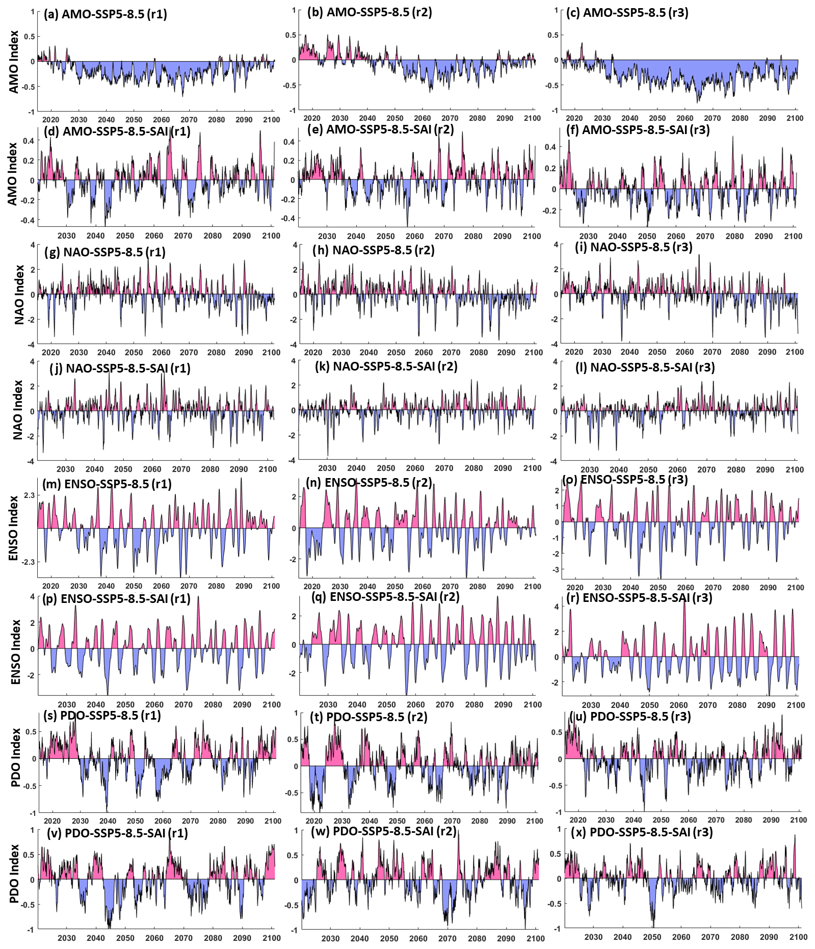
Figure 1The AMO (a–f), NAO (g–l), ENSO (i.e., NINO3.4, m–r), and PDO (s–x) indices obtained from ensemble members r1 (left column), r2 (middle column), and r3 (right column) of the SSP5-8.5 (odd rows) and SSP5-8.5-SAI (even rows) scenarios.
2.3 Spatiotemporal analyses
Analyses in both space and time as well as in modes of variability ranging from the inter-annual to decadal changes were used to identify the possible changes in the large-scale climate circulations resulting from global warming and SAI scenarios. EOF analysis is commonly used to extract the climate variability space–time modes (e.g., Chen and Tung, 2018; Joyce, 2002). We applied EOF to extract the first (dominant) modes of detrended non-seasonal SST and its corresponding variance across the North Atlantic and North Pacific, which are related to the AMO and PDO, respectively. As ENSO is the primary indicator of global climate variability, we used the leading EOF of global SST anomalies in the study of ENSO.
The continuous wavelet transform (CWT) is commonly used to capture the primary characteristics of signals (Addison, 2018). For a time series (xn, n=1, …, N) having regular time intervals δt, the CWT is computed as the convolution of xn with the scaled and normalized wavelet (e.g., here we use the Morlet wavelet, which gives reasonably equal weighting and resolution in time and period space; Grinsted et al., 2004):
where s is the wavelet scale, ψ0 the Morlet wavelet, ω0 dimensionless frequency, [*] the complex conjugate, and η dimensionless time. The noise spectrum assigned to generate significance testing is a key issue in time series analysis. We concurred with the widely used red-noise null hypothesis methodology based on 1000 synthetic series with the same mean, standard deviation, and first-order autoregressive coefficient as the target time series produced by Monte Carlo approaches to estimate the significance of the CWT (Grinsted et al., 2004). Additionally, for each time series, the CWT's global power spectrum was calculated as a function of time. The global power spectrum provides insight into the dominant temporal modes of variability of each climate index within each ensemble member for the reference GHG and SAI scenarios. The wavelet method cone of influence automatically shows where the periods analyzed are being influenced by the end of the time series. Thus, the longest periods can only be reliably assessed for the middle of the time series.
The individual ensemble members are treated as independent of each other in calculating the statistics of the ensembles. The CWT was conducted on monthly ENSO time series and the 12-month moving averaged low-pass filtered signals of the AMO, NAO, and PDO. We always use the longest available record length in every ensemble member to gain maximum statistical power to establish significant differences between experiments.
3.1 Changes in the spatial patterns
Figure 2 reveals the projected changes in the variance of the SST anomalies related to the AMO (i.e., across the North Atlantic), ENSO (i.e., global scale), and the PDO (i.e., across the North Pacific) based on CESM1 and CESM2 results. Figure S1 shows three different plots for the CESM1, as the time period of the 20-member ensemble for RCP8.5 differs: ensembles 001 to 003 (2010–2097) are longer than the other 17 ensemble members (2010–2030). For RCP8.5 and SSP5-8.5 using CESM1 and CESM2, respectively, the strong GHG forcing and global warming to the end of the 21st century increases the variance of the first EOF SST anomaly in the North Atlantic and North Pacific (representing the AMO and PDO) but reduces the variance of the leading EOF in global SST anomaly (related to ENSO). Based on the statistical t-test results, the changes in the means imposed by global warming relative to the historical period are all significant except one case (Fig. 2f). Differences between SAI and the historic period in CESM2 values of the leading EOF variance of the AMO and ENSO are not significant, showing that the significant changes under GHG forcing are effectively reversed by SAI. In contrast, the changes in the PDO variance imposed by global warming using CESM1 relative to historical period remain significant under SAI. Using CESM2, there is no significant changes in the PDO variance from the historical period to global warming or to SAI.

Figure 2Box and whisker plots of the variance in the leading EOFs, representing the AMO, the PDO, and ENSO, relative to the total variance of the SST fields: the AMO across the North Atlantic (a, b), ENSO (c, d) global SST, and the PDO across the North Pacific (e, f). The values in blue in each column box show the period of the data for historical, GHG (i.e., RCP-8.5 and SSP5-8.5), and climate intervention (GLENS-SAI and SSP5-8.5-SAI) scenarios. The titles of each subplot refer to the CESM version and the number of ensembles used in the historical, GHG (RCP8.5 and SSP5-8.5), and SAI (GLENS-SAI or SSP5-8.5-SAI) scenarios, respectively. The median for each experiment is denoted by the red line, the upper (75th) and lower (25th) quartiles by the top and bottom of the box, and ensemble limits by the whisker extents. The three values shown at the bottom of each subplot refer to the p values obtained from the statistical t test between historical and global warming, historical and SAI, and global warming and SAI, respectively. Values underlined are significant (i.e., p<0.05).
Figures 3–6 and S2–S3 show the spatial anomalies of the leading EOF mode of the SST in the North Atlantic, North Pacific, and tropical Pacific under both the CESM1 and CESM2. For the historical period, there is a cold-tongue pattern in the North Pacific broadens from the western to the eastern parts surrounded by warm water, particularly to the north. GHG-related global warming lowers the contrast between the cold-tongue pattern and its surroundings, increases the water temperature inside the cold-tongue pattern, and also leads to a substantial expansion of a warm pattern in the north. The same patterns (Fig. 4) are also obtained under SSP5-8.5 using CESM2. SAI effectively shrinks the warm pattern in the northern Atlantic under the RCP8.5 and SSP5-8.5 through a significant SST decrease, particularly using CESM1 (bottom row in Figs. 3 and 4). The SSP5-8.5-SAI experiment increases the temperature contrast in the cold-tongue pattern, while the GLENS-SAI does not. The projected changes in the spatial SST patterns across the North Atlantic, observed under global warming, are significantly suppressed under SAI (Figs. 3f and 4f). This response of the AMO to SAI is compatible with the observed changes in the AMO imposed by anthropogenic and volcanic aerosols reported by Masson-Delmotte et al. (2021). Anthropogenic and volcanic aerosols are understood to have impacted the timing and magnitude of the cold (negative) episode in the historical AMO record between the mid-1960s and mid-1990s and succeeding warming (Masson-Delmotte et al., 2021). Anthropogenic aerosols have also been suspected of impacting historical SSTs elsewhere, particularly the decadal ENSO variability (e.g., Sutton and Hodson, 2007; Westervelt et al., 2018).
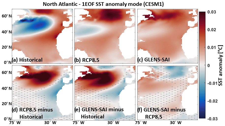
Figure 3The first EOF (1EOF) patterns of SST anomaly across the North Atlantic related to the AMO index simulated by CESM1 for the historical data (a) and the mean of the available ensemble member outputs under the RCP8.5 (b) and GLENS-SAI (c) scenarios. The maps in the bottom row show RCP8.5 minus historical (d), GLENS-SAI minus historical (e), and GLENS-SAI minus RCP8.5 (f) where the hatched patterns are not statistically significant (p>0.05), based on p values from t-test analysis.

Figure 4As in Fig. 3, but for CESM2 and SSP5-8.5.
The leading EOF of monthly global SST anomalies corresponding to the ENSO mode (Figs. S2 and S3 in the Supplement) is seen as a warm-tongue pattern over the tropical Pacific, which exhibits very similar patterns under both global warming and SAI scenarios as in the historical period. However, Fig. S4 shows that the warm-tongue pattern in CESM1 and CESM2 has an excessive westward extension relative to observations, which is compatible with the findings of Capotondi et al. (2020).
While the first EOF SST anomaly across the North Pacific under both global warming and SAI scenarios in CESM1 and CESM2 (Figs. 5 and 6) exhibits a similar cold-tongue pattern (typical of the North Pacific) as in the historical period, a lower contrast between the cold-tongue pattern and its surroundings is observed under SSP5-8.5 (Fig. 6b), which is effectively compensated by the geoengineering scenarios of SSP5-8.5-SAI through a significant SST decrease over the middle North Pacific (Fig. 6c and f), since there is no significant change between SAI and historical maps (Fig. 6e). There is an excessive eastward expansion of the cold-tongue pattern with cooler temperatures under the SAI scenario as simulated by the CESM1 (Fig. 5c), which is due to the significant cooling of the water in the outside of the cold-tongue pattern imposed by the SO2 injection (Fig. 5e–f).
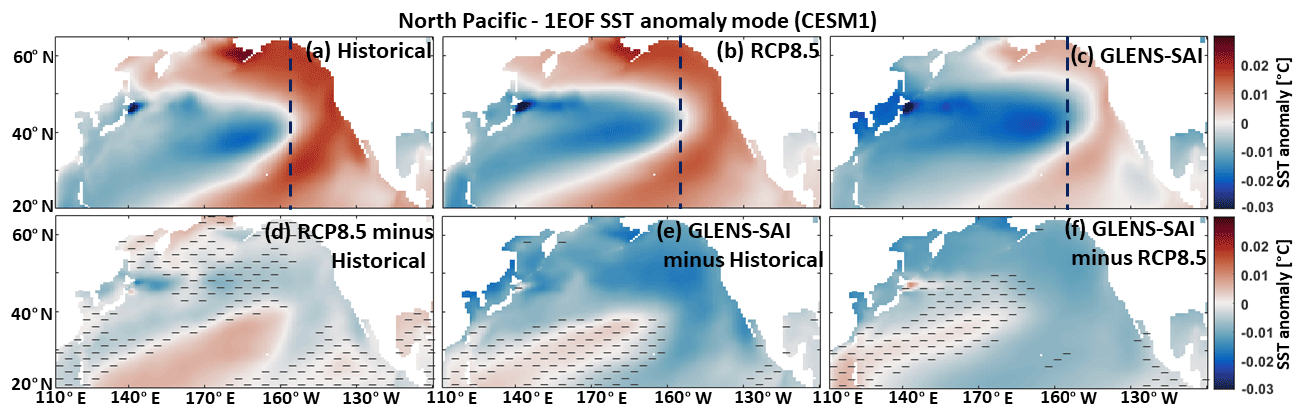
Figure 5As Fig. 3 but across the North Pacific related to the PDO index.
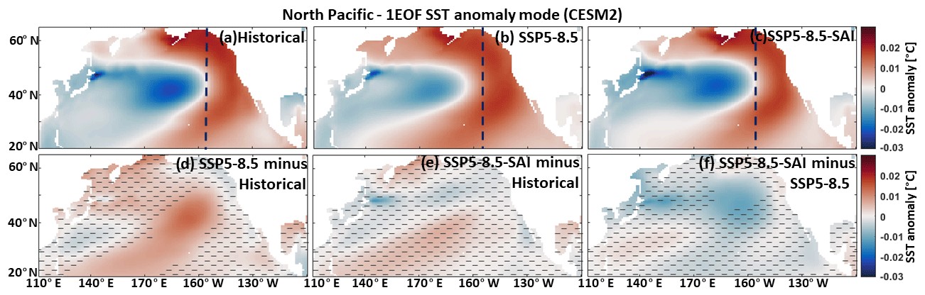
Figure 6As in Fig. 5 but for CESM2.
3.2 Temporal evolution of indices
Figure 7 displays the projected changes in the El Niño and La Niña episodes in the ENSO index under global warming and SAI. The global warming scenario simulated by CEMS2 tends to reduce the time between the La Niña episodes as well as the intensity and duration of the La Niña episodes compared to the historical conditions, but El Niño shows no significant changes. Frequency increases in both El Niño and La Niña episodes were suggested in earlier climate simulations, e.g., Fredriksen et al. (2020), Cai et al. (2014), and Yun et al. (2021) for El Niño and Cai et al. (2015) for La Niña. In contrast, using CESM1, the characteristic changes in El Niño are stronger than that in La Niño, and the El Niño intensity significantly increases, while its duration decreases relative to the historical period. The La Niña intensity significantly increases, but other characteristics show no significant changes under RCP8.5.
For CESM2, although SAI is mostly accompanied by a slight decrease in the median of El Niño and La Niña characteristics towards their historical value, its effect on global-warming-imposed changes is only statistically significant for the intensity and duration of La Niña events. For the CESM2 SAI experiment, there are no significant differences in El Niño characteristics as with the GHG forcing experiment. In contrast, La Niña peak intervals, height (i.e., intensity), and width (i.e., duration) characteristics are significantly different from GHG forcing and reverse the direction of changes imposed by GHG. For CESM1, there are no significant differences between the results from RCP8.5 and GLENS-SAI scenarios.
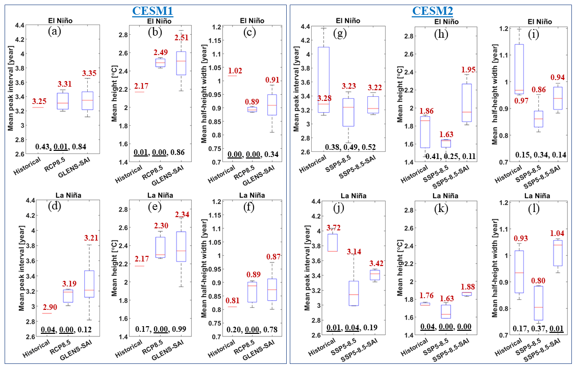
Figure 7The projected changes in the mean peak interval, height, and half-height width of El Niño and La Niña events for global warming (RCP8.5 and SSP5-8.5) and SAI (GLENS-SAI and SSP5-8.5-SAI) scenarios simulated by CESM1 (a–f) and CESM2 (g–l). The median for each experiment is denoted by the red line, the upper (75th) and lower (25th) quartiles by the top and bottom of the box, and ensemble limits by the whisker extents. The values labeled in red in each box show their median. The three values shown at the bottom of each subplot refer to the p values obtained from the statistical t test between historical and global warming, historical and SAI, and global warming and SAI, respectively. Values underlined are significant (i.e., p<0.05).
Another way to illustrate the temporal evolution of signals is by using the power spectrum. Figures 8 and S6 compare the changes in temporal variability of each climate index (AMO, NAO, ENSO, and PDO) using the global power spectrums of CWTs under global warming and SAI scenarios simulated by CESM2, excluding CESM1 outputs, as there is just a single ensemble member for CESM1 historical data over a short 1980–2009 period. In CESM1, the signals longer than decadal, which are the most energetic modes in observations of the PDO (Mantua and Hare, 2002) and AMO (Enfield et al., 2001), cannot be captured in the historical simulations owing to their short simulation period (1980–2009). As an example, Fig. S5 shows the ENSO CWTs and their global power spectrums for historical, SSP5-8.5, and SSP5-8.5-SAI scenarios.
The inter-annual modes of the AMO, the NAO, and ENSO are preserved under both global warming and SAI. For the decadal periodicities, SAI accentuates AMO changes induced by GHG (Fig. 8a). For example, the dominant modes at 20–30 years of the AMO, observed during the historical period, show no significant changes under global warming; however, they vanish under SAI. The decadal 10- to 20-year mode of the historical NAO is preserved neither in the global warming scenario nor with SAI (Fig. 8b). For ENSO, the dominant historical inter-annual modes show no significant change under both global warming and SAI, except that its power under SAI is stronger (Fig. 8c). The dominant modes at 10–20 years, observed in the historical PDO, are not present in both the SSP5-8.5 and SAI simulations, and the latter two are similar to each other (Fig. 8d). In contrast with the historical period in which the dominant modes of the PDO occur in the 10- to 20-year band, the dominant modes under global warming (i.e., SSP5-8.5) and SAI (i.e., SSP5-8.5-SAI) shift to a lower mode at the ∼8- to 13-year period. The PDO shift to a higher frequency with decadal variability weakness, observed under global warming, was also earlier demonstrated by Fang et al. (2014) with a previous generation of the climate model, the Fast Ocean Atmosphere Model (FOAM) used in IPCC AR4 experiments. Likewise, the PDO timescale has been simulated to decrease from ∼20 to ∼12 years under global warming (Fedorov et al., 2020), possibly because of changes in the phase speed of internal Rossby waves and ocean stratification (Zhang and Delworth, 2016).
We further analyzed the concatenated series from the available members for each scenario using CESM2 to statistically capture the low-frequency cycles with better reliability. Figure S6 summarizes the CWT global power spectrums for the AMO, the NAO, ENSO, and the PDO. The results, on the whole, are compatible with those shown in Fig. 8.

Figure 8The CWT global power spectrums obtained for the indices of the AMO (a), the NAO (b), ENSO (c), and the PDO (d) under SSP5-8.5 and SSP5-8.5-SAI relative to the historical results based on CESM2 for the periods of 1850–2014. Shading in each curve shows the across-ensemble range. The x axis in the NAO and ENSO graphs is on a logarithmic scale.
4.1 Caveats to interpretation
Caution is required when interpreting the results from this study with regard to real-world variability. Although CESM2 is highly rated among existing climate models, large model–observation differences are nonetheless present (Fasullo, 2020). Model–observation differences are larger in the earlier CESM1 version than in CESM2. For example, CESM1 exhibited a subtropical (Azores) High anomaly (related to the NAO) that was too weak, but its representation is improved in CESM2 (Simpson et al., 2020). We also find large differences in amplitude and variance of climate indices simulated by both CESM1 and CESM2 relative to the observations over the 1980–2009 period. The amplitude of the dominant EOF of the ENSO-related SST anomaly modeled in both CESM1 and CESM2 is about twice that of the observations for the historical (1980–2009) period (Figs. S4 and S7). Figure S7 further shows the NAO and PDO dominant-mode amplitudes are lower in the model projections than in observations over the historical period. Additionally, the ENSO-associated SST anomaly pattern in the tropical Pacific shows an excessive westward extension under both CESM1 and CESM2 (Fig. S4). These limitations mirror those by Capotondi et al. (2020) for CESM2 in simulating ENSO, who suggested further work to illuminate how the physical parameterizations impact the key ENSO feedback. Additionally, although CESM2 simulates the pattern of the summer and winter NAO well over the historical period 1979–2014, the large uncertainties in specific members and in the historical observations mean it is difficult to be quantitative about this (Simpson et al., 2020). However, CESM1 tends to underestimate the observed SST fluctuations in the Atlantic, leading to an underestimation of the forced response (Undorf et al., 2018).
CMIP models tend to systematically underestimate the low-frequency signals (i.e., PDO) in the North Pacific (Fasullo et al., 2020), owing in part to an imperfect modeling of decadal-scale structures in these simulations (Masson-Delmotte et al., 2021). Compared to observational estimates, the decadal variability in the subpolar North Atlantic SST appears to be slightly intensified through CMIP6 (Masson-Delmotte et al., 2021). How well we, therefore, can potentially capture forthcoming changes in climate indices' variability will be restricted by how good each model simulation is (Gabriel and Robock, 2015).
The second limitation is disparities in the length of records (30 (165) years for the historical period from CESM1 (CESM2), roughly ∼90 years for GHG emissions, and ∼80 years for SAI scenarios), which may hinder the direct comparison of climate indices' behavior between historical and future climate scenarios of global warming and SAI and thus the number of El Niño and La Niña events, as well as the significance of the longer periodicities (i.e., decadal and inter-decadal) in power spectrums. Furthermore, these records explore variability within the statistical assumptions of the methods, which may not be robust for non-stationary time series where the normality and independence assumptions inherent in the wavelet and t tests would not strictly hold. We are limited to the available simulations, and a three-member ensemble for SAI under CESM2 is inherently weaker than 20-member ensembles under CESM1. CESM1 has a shorter 30-year historical period from 1980 to 2009, which could not capture the longer than decadal variability modes of the teleconnection patterns. Yet another limitation arises from the relatively low spatial resolution of the models, which may affect the spatial SST anomaly patterns. Furthermore, Holmes et al. (2019) pointed out the models are too low resolution to resolve ocean eddies, which substantially contribute to ENSO irregularity and predictability. The absence of the eddy process may also be associated with bias in spatial patterns and other ENSO characteristics (Bellenger et al., 2014) in the CMIP models (Cai et al., 2021). Global high-horizontal-resolution climate models have been indicated to significantly improve the ocean–atmosphere circulations such as ENSO (Masson et al., 2012). As an example, Haarsma et al. (2016) pointed out that the High-Resolution Model Intercomparison Project for CMIP6 improves the understanding of the climate teleconnection patterns of large-scale circulations such as ENSO, the NAO, and the PDO, which suggests that running these high-resolution models with the SAI scenario would be worthwhile.
4.2 Implications for climate stability
Teleconnection signals represent emergent properties of the non-linear climate system. The behavior of the climate teleconnection patterns can be characterized via its oscillations. In its simplest form, a stable pattern would represent a fixed point or a periodic oscillation, but with real non-linear systems a quasi-periodic oscillation over specific frequency bands is more likely (e.g., Ghil et al., 2002). These quasi-periodic characteristic frequencies may change smoothly over time in a linear system but may proceed towards chaotic solutions via frequency doubling in non-linear systems. Moron et al. (1998) suggested that ENSO crossed a threshold in the early 1960s, and the periodicity of the seasonally forced climatic oscillator increased abruptly. Notably, a concomitant increase in the variance of the decadal band is consistent with abrupt frequency doubling. This can be expected in non-linear systems, as the energy in the system is raised, progressing along the pathway towards chaotic behavior and hence having less predictability on decadal timescales.
The impact of SAI on the energetics of the coupled system is to offset the GHG increases by design. Hence, we might expect that SAI could therefore reduce or stop the progression towards chaotic behavior. However, the real climate system is far more complex than a simple energy balance calculation. SAI increases stratospheric heating (Visioni et al., 2020), and this leads to tropospheric changes, especially in winds (Gertler et al., 2020), and tropical circulation (Cheng et al., 2022). Furthermore, the large heat reservoir of the global ocean has been out of equilibrium with the atmosphere for centuries of anthropogenic GHG emissions, and this excess heat cannot be dissipated by SAI within the timeframe in the simulations. So, we may expect SAI to, at best, imperfectly reverse the effects of GHG on teleconnections.
Ocean stratification (ocean buoyancy frequency) and the baroclinic Rossby wave in the North Pacific play significant roles in SST amplitude and PDO cycles, since enhanced ocean buoyancy frequency speeds up the Rossby waves, and so the decadal and longer cycle weakening accompanies higher PDO frequency (Fang et al., 2014). Ocean stratification changes predominantly in response to changes in surface temperature and salinity (Fang et al., 2014). The North Atlantic and the northeast Pacific are projected to be among those areas with the greatest stratification changes under global warming in the second half of the 21st century (Capotondi et al., 2012).
While SAI effectively reverses the changes in the spatial patterns under GHG forcing across the North Atlantic (i.e., AMO) and North Pacific (i.e., PDO) and compensates for modest changes in the characteristics of the El Niño and La Niña episodes (related to the tropical Pacific), it does not effectively suppress the projected changes in decadal (∼10- to 20-year) variability of circulations imposed by global warming. Anthropogenic aerosols intensify the inter-annual variability (particularly in ENSO) but weaken the longer than 10-year signals of the ocean–atmosphere circulations, compatible with the multiyear to decadal variations in the PDO (Hua et al., 2018). SAI involves aerosols in the stratosphere not the troposphere, so the effects will be different, not least because of stratospheric heating (Visioni et al., 2020). The cold-tongue patterns in the mid-latitude of both the North Atlantic and North Pacific tend to have an excess eastward extension under SAI, in line with the second phase of the North Pacific response to large volcanic eruptions (Wang et al., 2012), which are better analogues for SAI.
Whether the climate system in the model is representative of the Earth can be diagnosed to some extent by comparison of the historical simulation with observations. As noted in Sect. 4.1 both CESM versions do present differences from observations, so they are not perfect. All climate models are unavoidably uncertain (Knutti et al., 2002), mostly because of the imperfect understanding of many of the interplays and feedbacks within the climate system (Jun et al., 2008). Previous analysis of ENSO under SAI found no significant changes (Gabriel and Robock, 2015), but they used different models with widely varying fidelity of modeled ENSO to observations and much smaller simulated quantities of SO2 with the relatively modest RCP4.5 emissions scenario as a baseline. Furthermore, in the only previous assessment of ENSO under SAI, by Gabriel and Robock (2015), SAI simulations may not have been long enough to detect changes. The large 20-member ensemble of GLENS used in this study may overcome this limitation, especially for short-period indices, since this represents ∼1600 model years.
Changes in climate teleconnection patterns can indicate significant changes in the forcing. Such changes are seen in time series analysis of teleconnection indices in the real world that coincide with increased GHG (Tsonis et al., 2007; Wang et al., 2009). Wang et al. (2009) note that regime shifts in system behavior in the observations occurred when North Pacific and North Atlantic patterns increase their coupling, and the key instigator is the NAO. The historical NAO's decadal mode, which vanished under global warming in our analyses, is not restored by the simulated SAI.
The North Atlantic is an atypical region under SAI. The declines in heat transported northwards by AMOC under GHG forcing are, to a great extent, reversed under all kinds of SRM including SAI (Xie et al., 2022). Thus, great differences exist in SST and air–ocean heat flux between SAI and GHG climates in the North Atlantic (Yue et al., 2021). If regime shifts occur when North Atlantic and Pacific oceans increase their coupling, and if the decline in AMOC under GHG forcing decreases coupling between the basins, then SAI may act to promote regime shift by reversing a decline in AMOC.
Many authors have noted that explosive volcanism, in some ways a natural analogue for SAI, is accompanied by a positive episode of the NAO (e.g., Robock, 2000). Furthermore, in the extreme scenario of SAI being done, such that temperatures are actually decreased, then projected strengthening of AMOC occurs (Tjiputra et al., 2016). However, it is also possible that regime shifts induced by GHG forcing and the large temperature feedbacks they induce may dominate impacts over those fairly subtle regime shifts in climate teleconnection patterns.
This study delivers a first overview of SAI response to the large-scale ocean–atmosphere circulations of the AMO, the NAO, ENSO, and the PDO based on CESM1(WACCM), using the GLENS-SAI experiment, and CESM2(WACCM6), using the SSP5-8.5-SAI experiment, that apply stratospheric aerosol intervention through the injection of sulfur into the stratosphere. The impacts of these interventions are assessed against the historical period (1980–2009 for both models and 1850–2014 for CESM2 in some analyses) and projections under RCP8.5 and SSP5-8.5 (for the GLENS-SAI and SSP5-8.5-SAI, respectively). We found that SAI effectively reverses the global-warming-imposed changes in the variance of the leading EOF SST anomaly associated with the AMO, ENSO, and the PDO. SAI also effectively suppresses the changes in the spatial patterns of the EOF SST anomaly across the North Atlantic (i.e., AMO) and North Pacific (i.e., PDO). A decrease in the contrast between the cold-tongue pattern and its surroundings in the North Pacific is further projected under GHG-induced global warming, which the SAI successfully restored.
CESM2 simulations suggest that increasing GHG emissions are accompanied by a modest increase in the frequency of the El Niño and La Niña episodes but a modest decrease in their intensity and duration. The SAI scenario effectively compensates for these changes.
In contrast to the impact of the SAI on the spatial patterns of the climate indices of the AMO, the PDO, and ENSO, the SAI scenario does not effectively suppress the projected changes in decadal (∼10- to 20-year) variability imposed by global warming. The decadal variability modes of all the historical climate indices (except for Atlantic-based indices under SSP5-8.5) are not preserved in the GHG warming scenario, and SAI does not restore them.
Furthermore, compared to the historical 1850–2014 period in CESM2, SAI is projected to accentuate the AMO and to have no effective impact on the NAO at decadal frequencies. Unlike the historical period in which the long-period dominant modes of the PDO occur in the 10- to 20-year band, the dominant modes under global warming are reduced to ∼8–13 years, and SAI does not restore them.
The results exhibited here are particular to these types of future global warming scenarios and the details of the SAI application, which deal with an extreme scenario of GHG emissions and continuous increases in sulfur emissions. Furthermore, the findings are from ensemble members from just two closely related models. Caution is warranted due to the model–observation differences, disparities in the record length of the historical period compared to future climate scenarios, and the low spatial resolution of the models. Nevertheless, our study does detect changes in climate teleconnection signals and hence underlying climate system dynamics under SAI when decomposed using EOF and wavelet analyses.
The data for CESM1 and CESM2 simulations are publicly available via their websites: http://www.cesm.ucar.edu/projects/community-projects/GLENS/ (https://doi.org/10.5065/D6JH3JXX, NCAR, 2022) and https://esgf-node.llnl.gov/search/cmip6/ (CMIP6, 2022).
The supplement related to this article is available online at: https://doi.org/10.5194/acp-23-5835-2023-supplement.
AR: coordinated the analysis, graphics of various figures, and manuscript preparation; KK and ST: conceptualized and prepared the data; and JCM: conceptualized and coordinated the interpretation and discussion for various sections. All authors contributed to the discussion and writing.
The contact author has declared that none of the authors has any competing interests.
Publisher’s note: Copernicus Publications remains neutral with regard to jurisdictional claims in published maps and institutional affiliations.
We appreciate the financial support from the DEGREES Initiative in collaboration with the World Academy of Sciences (TWAS) under grant no. 4500443035. We further thank Gary Strand from NCAR for his help in accessing the CESM1 model outputs. Tan Mou Leong provided helpful comments and suggestions on the manuscript.
This research has been supported by the DEGREES Initiative in collaboration with the World Academy of Sciences (grant no. 4500443035).
This paper was edited by Peter Haynes and reviewed by two anonymous referees.
Abdelmoaty, H. M., Papalexiou, S. M., Rajulapati, C. R., and AghaKouchak, A.: Biases beyond the mean in CMIP6 extreme precipitation: A global investigation, Earth's Future, 9, e2021EF002196, https://doi.org/10.1029/2021EF002196, 2021.
Addison, P. S.: Introduction to redundancy rules: the continuous wavelet transform comes of age, Philos. T. Roy. Soc. A, 376, 20170258, https://doi.org/10.1098/rsta.2017.0258, 2018.
An, S. I. and Wang, B.: Inter-decadal change of the structure of the ENSO mode and its impact on the ENSO frequency, J. Climate, 13, 2044–2055, https://doi.org/10.1175/1520-0442(2000)013<2044:ICOTSO>2.0.CO;2, 2000.
Bellenger, H., Guilyardi, É., Leloup, J., Lengaigne, M., and Vialard, J.: ENSO representation in climate models: From CMIP3 to CMIP5, Clim. Dynam., 42, 1999–2018, https://doi.org/10.1007/s00382-013-1783-z, 2014.
Cai, W., Borlace, S., Lengaigne, M., Van Rensch, P., Collins, M., Vecchi, G., Timmermann, A., Santoso, A., McPhaden, M. J., Wu, L., and England, M. H.: Increasing frequency of extreme El Niño events due to greenhouse warming, Nat. Clim. Change, 4, 111–116, https://doi.org/10.1038/nclimate2100, 2014.
Cai, W., Wang, G., Santoso, A., McPhaden, M. J., Wu, L., Jin, F. F., Timmermann, A., Collins, M., Vecchi, G., Lengaigne, M., and England, M. H.: Increased frequency of extreme La Niña events under greenhouse warming, Nat. Clim. Change, 5, 132–137, https://doi.org/10.1038/nclimate2492, 2015.
Cai, W., Santoso, A., Collins, M., Dewitte, B., Karamperidou, C., Kug, J. S., Lengaigne, M., McPhaden, M. J., Stuecker, M. F., Taschetto, A. S., and Timmermann, A.: Changing El Niño–Southern Oscillation in a warming climate, Nature Reviews Earth & Environment, 2, 628–644, https://doi.org/10.1038/s43017-021-00199-z, 2021.
Capotondi, A. and Sardeshmukh, P. D.: Is El Niño really changing?, Geophys. Res. Lett., 44, 8548–8556, https://doi.org/10.1002/2017GL074515, 2017.
Capotondi, A., Alexander, M. A., Bond, N. A., Curchitser, E. N., and Scott, J. D., Enhanced upper ocean stratification with climate change in the CMIP3 models, J. Geophys. Res.-Oceans, 117, C04031, https://doi.org/10.1029/2011JC007409, 2012.
Capotondi, A., Deser, C., Phillips, A. S., Okumura, Y., and Larson, S. M.: ENSO and Pacific decadal variability in the Community Earth System Model version 2, J. Adv. Model. Earth Sy., 12, e2019MS002022, https://doi.org/10.1029/2019MS002022, 2020.
Chen, X. and Tung, K. K.: Global-mean surface temperature variability: Space–time perspective from rotated EOFs, Clim. Dynam., 51, 1719–1732, https://doi.org/10.1007/s00382-017-3979-0, 2018.
Cheng, L., Trenberth, K. E., Fasullo, J., Boyer, T., Abraham, J., and Zhu, J.: Improved estimates of ocean heat content from 1960 to 2015, Sci. Adv., 3, e1601545, https://doi.org/10.1126/sciadv.1601545, 2017.
Cheng, W., MacMartin, D. G., Kravitz, B., Visioni, D., Bednarz, E. M., Xu, Y., Luo, Y., Huang, L., Hu, Y., Staten, P. W., and Hitchcock, P.: Changes in Hadley circulation and intertropical convergence zone under strategic stratospheric aerosol geoengineering, npj Climate and Atmospheric Science, 5, 32, https://doi.org/10.1038/s41612-022-00254-6, 2022.
Cook, B. I., Mankin, J. S., Marvel, K., Williams, A. P., Smerdon, J. E., and Anchukaitis, K. J.: Twenty-first century drought projections in the CMIP6 forcing scenarios, Earth's Future, 8, e2019EF001461, https://doi.org/10.1029/2019EF001461, 2020.
Coupled Model Intercomparison Projects 6 (CMIP6): World Climate Research Programme, Department of Energy, Lawrence Livermore National Laboratory, https://esgf-node.llnl.gov/search/cmip6/ (last access: 1 December 2022), 2022.
Dagon, K. and Schrag, D. P.: Exploring the effects of solar radiation management on water cycling in a coupled land–atmosphere model, J. Climate, 29, 2635–2650, https://doi.org/10.1175/JCLI-D-15-0472.1, 2016.
Danabasoglu, G., Lamarque, J. F., Bacmeister, J., Bailey, D. A., DuVivier, A. K., Edwards, J., Emmons, L. K., Fasullo, J., Garcia, R., Gettelman, A., and Hannay, C.: The community earth system model version 2 (CESM2), J. Adv. Model. Earth Sy., 12, e2019MS001916, https://doi.org/10.1029/2019MS001916, 2020.
Enfield, D. B., Mestas-Nuñez, A. M., and Trimble, P. J.: The Atlantic multidecadal oscillation and its relation to rainfall and river flows in the continental US, Geophys. Res. Lett., 28, 2077–2080, https://doi.org/10.1029/2000GL012745, 2001.
Eyring, V., Bony, S., Meehl, G. A., Senior, C. A., Stevens, B., Stouffer, R. J., and Taylor, K. E.: Overview of the Coupled Model Intercomparison Project Phase 6 (CMIP6) experimental design and organization, Geosci. Model Dev., 9, 1937–1958, https://doi.org/10.5194/gmd-9-1937-2016, 2016.
Fang, C., Wu, L., and Zhang, X.: The impact of global warming on the Pacific Decadal Oscillation and the possible mechanism, Adv. Atmos. Sci., 31, 118–130, https://doi.org/10.1007/s00376-013-2260-7, 2014.
Fasullo, J. T. and Richter, J. H.: Dependence of strategic solar climate intervention on background scenario and model physics, Atmos. Chem. Phys., 23, 163–182, https://doi.org/10.5194/acp-23-163-2023, 2023.
Fasullo, J. T., Phillips, A. S., and Deser, C.: Evaluation of leading modes of climate variability in the CMIP archives, J. Climate, 33, 5527–5545, https://doi.org/10.1175/JCLI-D-19-1024.1, 2020.
Fedorov, A. V. and Philander, S. G.: A stability analysis of tropical ocean–atmosphere interactions: Bridging measurements and theory for El Niño, J. Climate, 14, 3086–3101, https://doi.org/10.1175/1520-0442(2001)014<3086:ASAOTO>2.0.CO;2, 2001.
Fedorov, A. V., Hu, S., Wittenberg, A. T., Levine, A. F., and Deser, C.: ENSO Low-Frequency Modulation and Mean State Interactions, El Niño Southern Oscillation in a changing climate, Geophysical Monograph Series, 173–198, https://doi.org/10.1002/9781119548164.ch8, 2020.
Field, C. B. and Barros, V. R. (Eds.): Climate change 2014–Impacts, adaptation and vulnerability: Regional aspects, Cambridge University Press, https://doi.org/10.1017/CBO9781107415386, 2014.
Fredriksen, H. B., Berner, J., Subramanian, A. C., and Capotondi, A.: How does El Niño–Southern Oscillation change under global warming–A first look at CMIP6, Geophys. Res. Lett., 47, e2020GL090640, https://doi.org/10.1029/2020GL090640, 2020.
Gabriel, C. J. and Robock, A.: Stratospheric geoengineering impacts on El Niño/Southern Oscillation, Atmos. Chem. Phys., 15, 11949–11966, https://doi.org/10.5194/acp-15-11949-2015, 2015.
Gertler, C. G., O'Gorman, P. A., Kravitz, B., Moore, J. C., Phipps, S. J., and Watanabe, S.: Weakening of the extratropical storm tracks in solar geoengineering scenarios, Geophys. Res. Lett., 47, e2020GL087348, https://doi.org/10.1029/2020GL087348, 2020.
Ghil, M., Allen, M. R., Dettinger, M. D., Ide, K., Kondrashov, D., Mann, M. E., Robertson, A. W., Saunders, A., Tian, Y., Varadi, F., and Yiou, P.: Advanced spectral methods for climatic time series, Rev. Geophys., 40, 3–39, https://doi.org/10.1029/2000RG000092, 2002.
Greene, C. A., Thirumalai, K., Kearney, K. A., Delgado, J. M., Schwanghart, W., Wolfenbarger, N. S., Thyng, K. M., Gwyther, D. E., Gardner, A. S., and Blankenship, D. D.: The climate data toolbox for MATLAB, Geochem. Geophy. Geosy., 20, 3774–3781, https://doi.org/10.1029/2019GC008392, 2019.
Grinsted, A., Moore, J. C., and Jevrejeva, S.: Application of the cross wavelet transform and wavelet coherence to geophysical time series, Nonlin. Processes Geophys., 11, 561–566, https://doi.org/10.5194/npg-11-561-2004, 2004.
Haarsma, R. J., Roberts, M. J., Vidale, P. L., Senior, C. A., Bellucci, A., Bao, Q., Chang, P., Corti, S., Fučkar, N. S., Guemas, V., von Hardenberg, J., Hazeleger, W., Kodama, C., Koenigk, T., Leung, L. R., Lu, J., Luo, J.-J., Mao, J., Mizielinski, M. S., Mizuta, R., Nobre, P., Satoh, M., Scoccimarro, E., Semmler, T., Small, J., and von Storch, J.-S.: High Resolution Model Intercomparison Project (HighResMIP v1.0) for CMIP6, Geosci. Model Dev., 9, 4185–4208, https://doi.org/10.5194/gmd-9-4185-2016, 2016.
Holmes, R. M., McGregor, S., Santoso, A., and England, M. H.: Contribution of tropical instability waves to ENSO irregularity, Clim. Dynam., 52, 1837–1855, https://doi.org/10.1007/s00382-018-4217-0, 2019.
Hu, Z. Z. and Wu, Z.: The intensification and shift of the annual North Atlantic Oscillation in a global warming scenario simulation, Tellus A, 56, 112–124, https://doi.org/10.3402/tellusa.v56i2.14403, 2004.
Hua, W., Dai, A., and Qin, M.: Contributions of internal variability and external forcing to the recent Pacific decadal variations, Geophys. Res. Lett., 45, 7084–7092, https://doi.org/10.1029/2018GL079033, 2018.
Intergovernmental Panel on Climate Change (IPCC): Working Group I Contribution to the Sixth Assessment Report (AR6), Climate Change 2021: The Physical Science Basis, 2021, https://www.ipcc.ch/assessment-report/ar6/ (last access: 5 December 2022), 2021.
Joyce, T. M.: One hundred plus years of wintertime climate variability in the eastern United States, J. Climate, 15, 1076–1086, https://doi.org/10.1175/1520-0442(2002)015<1076:OHPYOW>2.0.CO;2, 2002.
Jun, M., Knutti, R., and Nychka, D. W.: Spatial analysis to quantify numerical model bias and dependence: how many climate models are there?, J. Am. Stat. Assoc., 103, 934–947, https://doi.org/10.1198/016214507000001265, 2008.
Knutti, R., Stocker, T. F., Joos, F., and Plattner, G. K.: Constraints on radiative forcing and future climate change from observations and climate model ensembles, Nature, 416, 719–723, https://doi.org/10.1038/416719a, 2002.
Kravitz, B., Caldeira, K., Boucher, O., Robock, A., Rasch, P. J., Alterskjaer, K., Karam, D. B., Cole, J. N., Curry, C. L., Haywood, J. M., and Irvine, P. J.: Climate model response from the geoengineering model intercomparison project (GeoMIP), J. Geophys. Res.-Atmos., 118, 8320–8332, https://doi.org/10.1002/jgrd.50646, 2013.
Latif, M. and Keenlyside, N. S.: El Niño/Southern Oscillation response to global warming, P. Natl. Acad. Sci. USA, 106, 20578–20583, https://doi.org/10.1073/pnas.0710860105, 2009.
Mantua, N. and Hare, S.: The Pacific Decadal oscillation, J. Oceanogr., 58, 35–44, https://doi.org/10.1023/A:1015820616384, 2002.
Mantua, N. J., Hare, S. R., Zhang, Y., Wallace, J. M., and Francis, R. C.: A Pacific interdecadal climate oscillation with impacts on salmon production, B. Am. Meteorol. Soc., 78, 1069–1080, https://doi.org/10.1175/1520-0477(1997)078<1069:APICOW>2.0.CO;2, 1997.
Masson, S., Terray, P., Madec, G., Luo, J. J., Yamagata, T., and Takahashi, K.: Impact of intra-daily SST variability on ENSO characteristics in a coupled model, Clim. Dynam., 39, 681–707, https://doi.org/10.1007/s00382-011-1247-2, 2012.
Masson-Delmotte, V., Zhai, P., Pirani, A., Connors, S. L., Péan, C., Chen, Y., Goldfarb, L., Gomis, M. I., Matthews, J. B. R., Berger, S., Huang, M., Yelekci, O., Yu, R., Zhou, B., Lonnoy, E., Maycock, T. K., Waterfield, T., Leizell, K., and Caud, N.: Climate change 2021: the physical science basis, Contribution of working group I to the sixth assessment report of the intergovernmental panel on climate change, 2, https://10.1017/9781009157896, 2021.
Mills, M. J., Richter, J. H., Tilmes, S., Kravitz, B., MacMartin, D. G., Glanville, A. A., Tribbia, J. J., Lamarque, J. F., Vitt, F., Schmidt, A., and Gettelman, A.: Radiative and chemical response to interactive stratospheric sulfate aerosols in fully coupled CESM1(WACCM), J. Geophys. Res.-Atmos., 122, 13061–13078, https://doi.org/10.1002/2017JD027006, 2017.
Meinshausen, M., Lewis, J., McGlade, C., Gütschow, J., Nicholls, Z., Burdon, R., Cozzi, L., and Hackmann, B.: Realization of Paris Agreement pledges may limit warming just below 2∘ C, Nature, 604, 304–309, https://doi.org/10.1038/s41586-022-04553-z, 2022.
Moore, J. C., Rinke, A., Yu, X., Ji, D., Cui, X., Li, Y., Alterskjaer, K., Kristjánsson, J. E., Muri, H., Boucher, O., and Huneeus, N.: Arctic sea ice and atmospheric circulation under the GeoMIP G1 scenario, J. Geophys. Res.-Atmos., 119, 567–583, https://doi.org/10.1002/2013JD021060, 2014.
Moron, V., Vautard, R., and Ghil, M.: Trends, interdecadal and interannual oscillations in global sea-surface temperatures, Clim. Dynam., 14, 545–569, https://doi.org/10.1007/s003820050241, 1998.
National Center for Atmospheric Research (NCAR): Geoengineering Large Ensemble Project (GLENS), Comunity Earth System Model, https://doi.org/10.5065/D6JH3JXX, 2022.
Riahi, K., Rao, S., Krey, V., Cho, C., Chirkov, V., Fischer, G., Kindermann, G., Nakicenovic, N., and Rafaj, P.: RCP 8.5–A scenario of comparatively high greenhouse gas emissions, Climatic Change, 109, 33–57, https://doi.org/10.1007/s10584-011-0149-y, 2011.
Robock, A.: Volcanic eruptions and climate, Rev. Geophys., 38, 191–219, https://doi.org/10.1029/1998RG000054, 2000.
Scafetta, N.: Testing the CMIP6 GCM Simulations versus surface temperature records from 1980–1990 to 2011–2021: High ECS is not supported, Climate, 9, 161, https://doi.org/10.3390/cli9110161, 2021.
Simpkins, G.: Breaking down the NAO–AO connection, Nat. Rev. Earth Environ., 2, 88–88, https://doi.org/10.1038/s43017-021-00139-x, 2021.
Simpson, I. R., Bacmeister, J., Neale, R. B., Hannay, C., Gettelman, A., Garcia, R. R., Lauritzen, P. H., Marsh, D. R., Mills, M. J., Medeiros, B., and Richter, J. H.: An evaluation of the large-scale atmospheric circulation and its variability in CESM2 and other CMIP models, J. Geophys. Res.-Atmos., 125, e2020JD032835, https://doi.org/10.1029/2020JD032835, 2020.
Shukla, J.: Predictability in the midst of chaos: A scientific basis for climate forecasting, Science, 282, 728–731, https://doi.org/10.1126/science.282.5389.728, 1998.
Sutton, R. T. and Hodson, D. L.: Climate response to basin-scale warming and cooling of the North Atlantic Ocean, J. Climate, 20, 891–907, https://doi.org/10.1175/JCLI4038.1, 2007.
Tilmes, S., MacMartin, D. G., Lenaerts, J. T. M., van Kampenhout, L., Muntjewerf, L., Xia, L., Harrison, C. S., Krumhardt, K. M., Mills, M. J., Kravitz, B., and Robock, A.: Reaching 1.5 and 2.0 °C global surface temperature targets using stratospheric aerosol geoengineering, Earth Syst. Dynam., 11, 579–601, https://doi.org/10.5194/esd-11-579-2020, 2020.
Tjiputra, J. F., Grini, A., and Lee, H.: Impact of idealized future stratospheric aerosol injection on the large-scale ocean and land carbon cycles, J. Geophys. Res.-Biogeo., 121, 2–27, https://doi.org/10.1002/2015JG003045, 2016.
Trenberth, K. E.: The definition of El Niño, B. Am. Meteorol. Soc., 78, 2771–2778, https://doi.org/10.1175/1520-0477(1997)078<2771:TDOENO>2.0.CO;2, 1997.
Tsonis, A. A., Swanson, K., and Kravtsov, S.: A new dynamical mechanism for major climate shifts, Geophys. Res. Lett., 34, L13705, https://doi.org/10.1029/2007GL030288, 2007.
Undorf, S., Bollasina, M. A., Booth, B. B. B., and Hegerl, G. C.: Contrasting the effects of the 1850–1975 increase in sulphate aerosols from North America and Europe on the Atlantic in the CESM, Geophys. Res. Lett., 45, 11–930, https://doi.org/10.1029/2018GL079970, 2018.
Visioni, D., MacMartin, D. G., Kravitz, B., Lee, W., Simpson, I. R., and Richter, J. H.: Reduced poleward transport due to stratospheric heating under stratospheric aerosols geoengineering, Geophys. Res. Lett., 47, e2020GL089470, https://doi.org/10.1029/2020GL089470, 2020.
Wang, C. and Dong, S.: Is the basin-wide warming in the North Atlantic Ocean related to atmospheric carbon dioxide and global warming?, Geophys. Res. Lett., 37, L08707, https://doi.org/10.1029/2010GL042743, 2010.
Wang, G., Swanson, K. L., and Tsonis, A. A.: The pacemaker of major climate shifts, Geophys. Res. Lett., 36, L07708, https://doi.org/10.1029/2008GL036874, 2009.
Wang, T., Otterå, O. H., Gao, Y., and Wang, H.: The response of the North Pacific Decadal Variability to strong tropical volcanic eruptions, Clim. Dynam., 39, 2917–2936, https://doi.org/10.1007/s00382-012-1373-5, 2012.
Watson, A. J., Schuster, U., Bakker, D. C., Bates, N. R., Corbière, A., González-Dávila, M., Friedrich, T., Hauck, J., Heinze, C., Johannessen, T., and Körtzinger, A.: Tracking the variable North Atlantic sink for atmospheric CO2, Science, 326, 1391–1393, https://doi.org/10.1126/science.1177394, 2009.
Westervelt, D. M., Conley, A. J., Fiore, A. M., Lamarque, J.-F., Shindell, D. T., Previdi, M., Mascioli, N. R., Faluvegi, G., Correa, G., and Horowitz, L. W.: Connecting regional aerosol emissions reductions to local and remote precipitation responses, Atmos. Chem. Phys., 18, 12461–12475, https://doi.org/10.5194/acp-18-12461-2018, 2018.
Xie, M., Moore, J. C., Zhao, L., Wolovick, M., and Muri, H.: Impacts of three types of solar geoengineering on the Atlantic Meridional Overturning Circulation, Atmos. Chem. Phys., 22, 4581–4597, https://doi.org/10.5194/acp-22-4581-2022, 2022.
Yue, C., Schmidt, L. S., Zhao, L., Wolovick, M., and Moore, J. C.: Vatnajökull mass loss under solar geoengineering due to the North Atlantic meridional overturning circulation, Earth's Future, 9, e2021EF002052, https://doi.org/10.1029/2021EF002052, 2021.
Yun, K. S., Lee, J. Y., Timmermann, A., Stein, K., Stuecker, M. F., Fyfe, J. C., and Chung, E. S.: Increasing ENSO–rainfall variability due to changes in future tropical temperature–rainfall relationship, Communications Earth & Environment, 2, 1–7, https://doi.org/10.1038/s43247-021-00108-8, 2021.
Zhang, L. and Delworth, T. L.: Simulated response of the Pacific decadal oscillation to climate change, J. Climate, 29, 5999–6018, https://doi.org/10.1175/JCLI-D-15-0690.1, 2016.
Zhang, R. and Delworth, T. L.: Impact of Atlantic multidecadal oscillations on India/Sahel rainfall and Atlantic hurricanes, Geophys. Res. Lett., 33, L17712, https://doi.org/10.1029/2006GL026267, 2006.